On the Singularity Structure and Stability of Plane Waves

Abstract:

We describe various aspects of plane wave backgrounds. In particular, we make explicit a simple criterion for singularity by establishing a relation between Brinkmann metric entries and diffeomorphism-invariant curvature information. We also address the stability of plane wave backgrounds by analyzing the fluctuations of generic scalar modes. We focus our attention on cases where after fixing the light-cone gauge the resulting world sheet fields appear to have negative “mass terms”. We nevertheless argue that these backgrounds may be stable.

1 Introduction and summary

Plane wave spacetimes have special properties that motivate their study in both General Relativity and string theory. Due to the presence of a covariantly constant null Killing vector and the specific structure of the curvature invariants, it was suggested early on that $\alpha^{\prime}$ corrections were under control for stringy plane wave backgrounds. Along these lines some concrete realizations were found in the context of WZW models providing examples of exact strings backgrounds on curved spacetimes [1] (see [2] and references therein). More recently, renewed interest in plane wave backgrounds has resulted from the realization that certain plane wave backgrounds are maximally supersymmetric solutions of eleven dimensional and IIB supergravity [3, 4] (see also [5]). More remarkable is the fact that some of these backgrounds allow for exact quantization in the light-cone gauge [6] (see also [7]), thus providing examples of tractable string theory backgrounds with Ramond-Ramond (RR) fluxes on curved spacetimes. Finally, based on the fact that some of the maximally supersymmetric plane waves can be obtained as Penrose-Güven limits [8, 9] of $AdS_{p}\times S^{q}$ backgrounds [10], a gauge theory interpretation based on the AdS/CFT correspondence was proposed in [11].

These special properties have motivated the study of many generalizations. One particularly prolific direction is the study of Penrose limits of known supergravity backgrounds. The Penrose limit, generalized to include form fields and fermions by Güven, yields a plane wave metric. Some of these metrics are known, however many present new and unexpected features. This situation motivated us to study a fairly general class of such backgrounds.

A particular class of interest are metrics which in the string frame have the so-called Brinkmann [12] form

$$ds^{2}=-4dx^{+}dx^{-}-(x^{i}\mu^{2}_{ij}x^{j})(dx^{+})^{2}+\delta_{ij}dx^{i}dx^{j},$$ (1)

where the matrix $\mu^{2}_{ij}$ is an arbitrary function of $x^{+}$. Any other fields should depend only on the coordinate $x^{+}$. Furthermore, the field strengths of any gauge fields should annihilate the vector field $\frac{\partial}{\partial x^{-}}$. It is clear that the $x^{-}$ translation $x^{-}\rightarrow x^{-}+\epsilon$ with all other coordinates held constant is a symmetry, so that $\frac{\partial}{\partial x^{-}}$ is a (null) Killing field.

We are interested in two very natural questions that arise in the context of Penrose limits of string theory backgrounds: (i) When is a plane wave metric singular? (ii) When is a plane wave background stable? Since scalar curvature invariants vanish for plane waves, it is useful to identify diffeomorphism invariant characterizations of the properties of (1). The question of stability appears when some of the eigenvalues of the matrix $\mu^{2}_{ij}$ are negative. Some comments on these backgrounds have already appeared in [13, 14, 15]. The case where $\mu^{2}_{ij}$ has at least one negative eigenvalue is interesting because this seems to imply the existence of worldsheet tachyonic fields. Physically, such negative eigenvalues of $\mu_{ij}^{2}$ imply that objects are stretched and separated by gravitational tidal forces. The effect is similar to that felt in de Sitter space, though without the formation of horizons.

In section 2 we make explicit a criterion for detecting curvature singularities in plane wave backgrounds by explicitly relating a diffeomorphism invariant object to the structure of the metric. Our criterion provides an immediate answer to the question of the singularity structure.

The question of stability is most cleanly formulated in time-independent settings. For this reason, we focus mainly on the case where $\mu_{ij}^{2}$ is independent of $x^{+}$. In section 3, we consider a scalar mode as a typical example of a perturbation. We study both the classical dynamics and quantization in plane wave backgrounds. We refer the reader to [16] for a stability analysis of other supergravity fields. We then proceed to stringy issues in section 4. In the discussion section we point out a number of open issues concerning string interactions. Our work has a certain overlap with that of [16], though the results were obtained independently and simultaneously.

2 Plane waves: Singular or Regular

In order to arrive at a criterion for regularity we need to describe some aspects of the geometry of plane waves. We proceed quickly since most of these results are at least implicitly discussed in the literature (especially in the classic works [12, 17, 18, 19, 20, 21]). Nevertheless, it is useful to have such results in explicit form.

2.1 Symmetries

Any metric of the Brinkmann form (1) has a rather high degree of symmetry. Killing’s equation is:

$$0=\xi_{\mu;\nu}+\xi_{\nu;\mu}=\partial_{\nu}\xi_{\mu}+\partial_{\mu}\xi_{\nu}-2\Gamma_{\nu\mu}^{\alpha}\xi_{\alpha},$$ (2)

and the only nonzero Christoffel symbols (with all indices down) are

$$\Gamma_{++i} = -\mu^{2}_{ij}x^{j}=-\Gamma_{i++},$$ (3)

$$\Gamma_{+++} = -\frac{1}{2}x^{i}\bigl{(}\frac{\partial}{\partial x^{+}}\mu^{2}_{ij}\bigr{)}x^{j},$$ (4)

We use the conventions of Misner, Thorne, and Wheeler [22].

Consider a Killing field with $\xi_{-}=0$ and with $\xi_{i}$ a function only of $x^{+}$. A lengthy but straightforward calculation shows that all Killing fields in fact satisfy the first of these conditions while the second condition holds for all Killing fields except for possible rotational symmetries of $\mu_{ij}$. Given these conditions, Killing’s equation reduces to

$$\partial_{+}\xi_{+}=x^{i}\mu^{2}_{ij}\xi^{j}, \ \ \ \rm{and}$$ (5)

$$\partial_{+}\xi_{i}+\partial_{i}\xi_{+}=0.$$ (6)

Latin indices are freely raised and lowered with the flat Euclidean metric $\delta_{ij}$. Combining the above two equations yields

$$\partial_{+}^{2}\xi_{i}+\mu^{2}_{ij}\xi^{j}=0,$$ (7)

which has solutions for all initial data $\xi^{i}(0)$, $\partial_{+}\xi^{i}(0)$. The general solution for $\xi_{+}$ is then given by

$$\xi_{+}=-x^{i}\partial_{+}\xi_{i}+c,$$ (8)

where $c$ is an arbitrary constant. Note that we have identified enough Killing fields to show that each null surface $x^{+}=constant$ is a homogeneous surface.

The detailed properties of the Killing fields depend on the choice of initial data. For definiteness, let us consider the time independent case, where $\partial_{+}$ is also a Killing field. Then the $\xi^{i}$ form a collection of harmonic or inverted harmonic oscillators. Some choices of initial data thus lead to ‘corkscrew’ motions which wind or rotate around the origin. Such Killing fields are no doubt related to the rotating D-branes of [23].

2.2 Geodesics and Curvatures

Let us now consider the curve $x^{i}=0,x^{-}=0$. Since the metric (1) is symmetric under the reflection $(x^{i},x^{-},x^{+})\rightarrow(-x^{i},-x^{-},-x^{+})$, an acceleration vector for this curve at $x^{+}=0$ must be invariant under this symmetry. As a result, this vector can point only along the curve. But since the origin of $x^{+}$ is arbitrary, we see that the curve is a geodesic. Direct calculation then shows that $x^{+}$ is an associated affine parameter.

A large family of null geodesics can be obtained by applying symmetries to the curve $x^{i}=0,x^{-}=0;$ i.e., by acting with the translation $e^{\xi}$. These geodesics satisfy $x^{+}=\lambda$, $x^{-}=\frac{1}{4}(\xi^{i}\partial_{+}\xi_{i})-c$, and $x^{i}(x^{+})=\xi^{i}(x^{+})$ with $\lambda$ an affine parameter and $\xi$ some Killing field of the form discussed in section 2.1. The fact that these curves trace out geodesics explains why equation (7) will look familiar to readers who have not previously studied the Killing symmetries of these spacetimes but who have studied geodesic motion. This family contains all of the null geodesics except those that follow the orbits of $\frac{\partial}{\partial x^{-}}$.

Suppose that two geodesics are related by a flow through a unit Killing parameter along some Killing field ${\bf\xi}$ of the form described in section 2.1. Then the distance separating these geodesics along any surface $x^{+}=constant$ is given by $|{\bf\xi}|=\sqrt{|\sum_{i}\xi^{i}\xi^{i}|^{2}}.$ Since $x^{+}$ is an affine parameter for this family of geodesics, it is also meaningful to speak of the relative velocity $\partial_{+}\xi^{\alpha}$ and acceleration $\partial_{+}^{2}\xi^{\beta}$ of these geodesics, so long as we keep in mind the freedom to rescale any affine parameter by an overall (i.e., $x^{+}$ independent) constant and to shift its origin. In particular, this information is diffeomorphsim invariant modulo the potential scaling and shift. Note that these relative accelerations measure gravitational tidal forces and, if the geodesics are infinitesimally separated, they are given by certain components of the Riemann tensor:

$$\partial^{2}_{+}\xi^{\nu}=-R_{\alpha\beta\gamma}^{\nu}\xi^{\beta}t^{\alpha}t^{\gamma},$$ (9)

where $t^{\alpha}$ is the tangent vector to the geodesic. If we take one of the geodesics to be at $x^{i}=0$, then this tangent vector is just $t^{\alpha}\partial_{\alpha}=\frac{\partial}{\partial x^{+}}$.

Thus for Killing vector fields $\xi$ and $\xi^{\prime}$ we have

$$\xi^{i}\mu_{ij}^{2}\xi^{\prime}{}^{j}=-\xi_{i}\partial_{+}^{2}\xi^{\prime}{}^{i}=\xi_{\nu}R_{\alpha\beta\gamma}^{\nu}\xi^{\prime}{}^{\beta}t^{\alpha}t^{\gamma},$$ (10)

so that the matrix-valued function $\mu^{2}_{ij}(x^{+})=R_{i+j+}(x^{+})$ describes diffeomorphism-invariant curvature information (up to an overall scale and shift of the origin of $x^{+}$). In particular, the divergence of any component of $\mu^{2}_{ij}$ at some value of $x^{+}$ represents a singularity where invariantly defined components of the curvature tensor diverge.

2.3 Penrose Limit of Schwarzschild Black Hole in AdS

Taking the Penrose limit of supergravity backgrounds dual to gauge theories with a mass scale has been one of the most natural generalizations of the BMN construction. In most cases intuition from the field theory side has helped in clarifying the effect of the Penrose limit on the original background. However, a universal understanding of the Penrose limit in intrinsically gravitational terms is lacking in the recent literature. Here we elaborate on a concrete example – the Schwarzschild black hole in AdS. Our intention is to provide a careful interpretation of the effect of the limit on the original background along the lines of the work by Geroch [26]. This approach was implicitly assumed also in [5].

The metric we consider is

$$ds^{2}=-({r^{2}\over R^{2}}+1-{M\over r^{2}})dt^{2}+({r^{2}\over R^{2}}+1-{M\over r^{2}})^{-1}dr^{2}+r^{2}d\Omega_{3}^{2}+R^{2}\bigg{[}d\psi^{2}+\sin^{2}\psi d\Omega_{4}^{2}\bigg{]}.$$ (11)

The above metric describes the Schwarzschild black hole in AdS in global coordinates. To perform the Penrose limit we consider a null geodesic in the directions determined by $(t,r,\psi)$. The effective Lagrangian that is equivalent to solving the geodesic equations is:

$${\cal L}=-({r^{2}\over R^{2}}+1-{M\over r^{2}})\dot{t}^{2}+({r^{2}\over R^{2}}+1-{M\over r^{2}})^{-1}\dot{r}^{2}+R^{2}\dot{\psi}^{2},$$ (12)

where dot represents derivative with respect to the affine parameter $U$. The aim is, following Penrose’s prescription [8](see also [5]), to find new coordinates $(U,V,Y^{i})$ where the metric takes the form

$$ds^{2}=dV(2dU+\alpha dV+\beta_{i}dY^{i})+C_{ij}dY^{i}dY^{j},$$ (13)

where $\alpha,\beta_{i}$ and $C_{ij}$ depend on all the the coordinates. Once the metric is in this form the Penrose limit is given by the scalings

$$ds^{2}=\Omega^{-2}ds^{2}(\Omega),\quad U=u,\quad V=\Omega^{2}v,\quad Y^{i}=\Omega y^{i},\quad\Omega\to 0.$$ (14)

Note that $\partial_{U}$ is a null vector since

$$g_{UU}=G_{tt}\dot{t}^{2}+G_{rr}\dot{r}^{2}+G_{\psi\psi}\dot{\psi}^{2}=0$$ (15)

by definition of a null geodesic. The equations of motion following from (12) are particularly simple since the effective Lagrangian does not depend explicitly on $t$ or $\psi$:

$$\dot{\psi}={\mu\over R^{2}},\quad\dot{t}={E\over{r^{2}\over R^{2}}+1-{M\over r^{2}}},\quad\dot{r}^{2}+{\mu^{2}\over R^{4}}r^{2}-{\mu^{2}\,M\over R^{2}\,r^{2}}=E^{2}-{\mu^{2}\over R^{2}}.$$ (16)

These three equations completely determine the dependence of the coordinates $(r,t,\psi)$ on the affine parameter $U$. To complete the coordinate transformation we use the conditions that $G_{UV}=1$ and $G_{U\Phi}=0$. The final coordinate change is the of the form

$$r=r_{U},\quad t=t_{U}-{V\over E}+\mu\Phi,\quad\psi={\mu\over R^{2}}U+E\Phi,$$ (17)

where $r_{U}$ and $t_{U}$ are functions only of $U$ determined by (16). Taking the Penrose limit following (14) we find the following metric in Rosen coordinates

$$ds^{2}=2dudv+(E^{2}R^{2}-\mu^{2}f(r))d\phi^{2}+r^{2}ds^{2}({\bf R}^{3})+R^{2}\sin^{2}({\mu\over R^{2}}U)ds^{2}({\bf R}^{4}),$$ (18)

where $f(r)={r^{2}\over R^{2}}+1-{M\over r^{2}}$ and $r$ is related to $u$ as

$$2{\mu\over R^{2}}u=\arctan{\mu r^{2}/R^{2}-E^{2}R^{2}/2\mu\over\sqrt{(E^{2}-{\mu^{2}\over R^{2}})r^{2}-{\mu^{2}\over R^{4}}r^{4}+{\mu^{2}M\over R^{2}}}}.$$ (19)

An arbitrary metric in Rosen coordinates

$$ds^{2}=2dudv+C_{ij}(u)dy^{i}dy^{j},$$ (20)

can be presented in Brinkmann form

$$ds^{2}=-4dx^{+}dx^{-}+\bigg{[}\sum\limits_{i,j}A_{ij}(x^{+})x^{i}x^{j}\bigg{]}(dx^{+})^{2}+\sum\limits_{i}dx^{i}dx^{i},$$ (21)

by means of the following coordinate transformation:

$$u=2x^{+},\quad v=x^{-}-{1\over 2}\sum\limits_{i,j}M_{ij}(x^{+})x^{i}x^{j},\quad y^{i}=\sum\limits_{i}Q^{i}_{j}(x^{+})x^{j}$$ (22)

where

$$C_{ij}Q^{i}_{k}Q^{j}_{l}=\delta_{kl},\quad C_{ij}(Q^{\prime}{}^{i}_{j}Q^{j}_{l}-Q^{\prime}{}^{i}_{k}Q^{j}_{l})=0,\quad M_{ij}=C_{kl}Q^{\prime}{}^{k}_{l}Q^{l}_{j},$$ (23)

where prime indicates derivative with respect to $x^{+}$. In the particular case when $C_{ij}=a^{2}_{i}(x^{+})\delta_{ij}$ is diagonal we have that

$$A_{ij}={(a_{i}(x^{+}))^{\prime\prime}\over a_{i}(x^{+})}\delta_{ij}$$ (24)

For the Schwarzschild black hole we obtain a metric that can be written in Brinkmann coordinates as:

$$ds^{2}=-4dx^{+}dx^{-}-{\mu^{2}\over R^{4}}\bigg{[}\sum\limits_{a=1}^{4}x_{a}^{2}+(1+{MR^{2}\over r^{4}})\sum\limits_{b=5}^{7}x_{b}^{2}+(1-3{MR^{2}\over r^{4}})x_{8}^{2}\bigg{]}(dx^{+})^{2}+\sum\limits_{i=1}^{8}dx_{i}^{2}$$ (25)

One question that naturally arises when considering Penrose limits of metrics containing dimensionful parameters is what happens to these parameters under the rescaling. In what follows we address this question in the specific case of AdS-Schwarzschild but our approach is universal. First, note that the Penrose limit can be thought of in two parts (performed simultaneously). One is an overall scaling of the metric by $\Omega^{-2}$. This takes the original spacetime $ds^{2}$ to a physically different spacetime $ds^{2}_{\Omega}=\Omega^{-2}ds^{2}$. In the case at hand, it takes us from one AdS-Schwarzschild metric to another. Now, the cosmological constant and black hole mass are diffeomorphism-invariant quantities. Suppose we calculate the cosmological constant and black hole mass from $ds^{2}_{\Omega}$ and use these to define the ($\Omega$-dependent) quantities $R_{\Omega}$ and $M_{\Omega}$. Then dimensional analysis is enough to tell us that we have

$$R_{\Omega}=R/\Omega$$ (26)

and

$$M_{\Omega}=M/\Omega^{2}.$$ (27)

Note that these two parts are interpreted differently in the dual field theory. The rescaling of the metric and corresponding change from one spacetime to another requires that we alter the dual field theory to match. In particular, we must take $g_{YM}N$ in the field theory to become infinitely large in a way that matches $R_{\Omega}$. This is the content of the statement “$R=\Omega^{-1}$” commonly associated with this limit [11]. In particular, one does not rescale $R$ in addition to taking the Penrose limit; rather, the rescaling of $R$ is a consequence of interpreting the strict Penrose limit in the dual field theory. Tracing through the duality map should also tell us on the field theory side how the temperature of the thermal bath corresponding to the black hole varies with $\Omega$. Not surprisingly, we find that the temperature of the black hole is $T_{\Omega}=\Omega T$ and therefore goes to zero in the limit as is compatible with our knowledge that the “black hole” disappears (see [29] for a discussion of the possibility of black holes in plane waves).

In much the same way that we defined $M_{\Omega}$ and $R_{\Omega}$ above, one may define $E_{\Omega}$ and $\mu_{\Omega}$ by calculating them from (16) applied to the favored null geodesic in the spacetime $ds^{2}_{\Omega}$. The key point is that the geodesic remains the same in terms of the coordinates $\tilde{t}=t/R,\tilde{r}=r/R,$ and $\psi$ and that the parametrization remains unchanged (we always use affine parameter $U$). (The geodesic also remains unchanged in terms of $t,r,\psi$, but $\tilde{t},\tilde{r},$ and $\psi$ are nicer as the rescaled metric maintains the same form except for the replacement of $R$ with $R_{\Omega}$.) Thus, $\dot{\psi}=\mu/R^{2}$ is independent of $\Omega$ and $\dot{\tilde{t}}=E/f(r)R$ is independent of $\Omega$. In other words, we may identify

$$E_{\Omega}=E/\Omega$$ (28)

and

$$\mu_{\Omega}=\Omega^{-2}\mu.$$ (29)

It is natural to assert that such scalings are the supergravity dual of the statement on the field theory side that we are focusing on states with large energy and large R-charge.

To further simplify the above metric we introduce $q=ER/\mu$ and $\tilde{r}=r/(qR)$ and $\tilde{m}=M/(qR^{2})$. Then we have

$$ds^{2}=-4dx^{+}dx^{-}-\bigg{[}\sum\limits_{a=1}^{4}x_{a}^{2}+(1+{\tilde{m}\over{\tilde{r}}^{4}})\sum\limits_{b=5}^{7}x_{b}^{2}+(1-3{\tilde{m}\over{\tilde{r}}^{4}})x_{8}^{2}\bigg{]}(d{{\mu x^{+}}\over R^{2}})^{2}+\sum\limits_{i=1}^{8}dx_{i}^{2}.$$ (30)

Furthermore, note that the equation (19) relating $u$ and $r$ can be written:

$${{\mu x^{+}}\over R^{2}}=\arctan{{\tilde{r}^{2}-1/2}\over{\tilde{r}^{2}-\tilde{r}^{4}+\tilde{m}}},$$ (31)

so that the entire final metric is specified by the parameter $\tilde{m}$. It is worth noting that the same background is obtained as the limit of non-extremal D3-branes in Poincare coordinates. Now we have an answer to the question of what happened to the $r=0$ singularity of the original black hole. According to the criterion above, a singularity remains at $r=0$ in the Penrose limit.

3 Field theory on plane waves with negative eigenvalues

One of the intriguing features of the background (30) is the negative eigenvalue (associated with $x_{8}$) of the matrix $\mu^{2}_{ij}$ that arises for small $r$. If one attempts to quantize string theory in the light-cone gauge on the background (30) one would have a negative “mass term” for the worldsheet boson $x_{8}$. One might wonder whether this is a tachyonic instability. The appearance of these negative “mass terms” is commonplace when studying Penrose limits of backgrounds with a mass scale [13, 27].

Here we investigate plane wave backgrounds in the field theory approximation. To be specific, we assume that the spacetime (1) is a classical solution to some gravitating theory and consider small perturbations about this background. For definiteness, we assume that the perturbations can be modeled by massless scalars. Below, we consider the case where the matrix $\mu^{2}_{ij}$ has at least one negative eigenvalue. The weak energy condition then implies that $\mu^{2}_{ij}$ also has at least one positive eigenvalue.

Let us take a moment to put our problem into perspective. Our real concern is the stability of the spacetime. This concern is raised by the negative eigenvalues of $\mu^{2}_{ij}$, which for example appear as negative mass-squared terms in the light-cone string sigma-model. One might therefore think that our spacetime has tachyonic perturbations. But such perturbations can be identified in a classical stability analysis. As a result, one would expect that the most important features can be seen directly in a classical analysis of linear fields propagating on the plane wave background. One would also expect such perturbations to be qualitatively similar for all massless fields. Indeed, while we will return to quantum effects in section 3.3 and to string effects in section 4, in the end we will see that the most important features are captured by the classical massless scalar field which we investigate below.

3.1 Massless classical field theory on the plane-wave spacetime

Consider a massless scalar field minimally coupled to the string metric. Such a field satisfies the equation of motion

$$\nabla^{2}\phi=0,$$ (32)

where $\nabla^{2}$ is the Laplace-Beltrami operator associated with the string metric. Recall that the curvature scalar $R$ and the squared field strength $F^{2}$ of any gauge field both vanish in our background. Thus, dilaton perturbations also satisfy (32), as do scalar fields with arbitrary curvature couplings. Perturbations of other supergravity fields are discussed in [16], where it is shown that their equations of motion take a similar form in an appropriate gauge.

For the metric (1), the wave equation (32) is proportional to the condition

$$[-4\partial_{-}\partial_{+}+(x^{i}\mu^{2}_{ij}x^{j})\partial_{-}^{2}+4\delta^{ij}\partial_{i}\partial_{j}]\phi=0.$$ (33)

It is convenient to expand $\phi$ in a basis of modes. Let us consider first the case where $\mu^{2}_{ij}$ is independent of $x^{+}$, so that it makes sense to choose modes $\phi_{p_{-},p_{+},\beta}$ which satisfy

$$\partial_{-}\phi_{p_{-},p_{+},\beta} = ip_{-}\phi_{p_{-},p_{+},\beta},\ \ \ {\rm and}$$ (34)

$$\partial_{+}\phi_{p_{-},p_{+},\beta} = ip_{+}\phi_{p_{-},p_{+},\beta}.$$ (35)

Here, $\beta$ is any index that labels the remaining degeneracy of the modes. If desired, explicit solutions are readily obtained in terms of Hermite polynomials.

The central question is whether such perturbations are stable. In other words, we must ask whether there can be a complete set of modes $\phi_{p_{-},p_{+},\beta}$ with real $p_{+},p_{-}$. The fact that the ‘mass term’ $(x^{i}\mu^{2}_{ij}x^{j})$ in (33) can be negative suggests that complex frequencies may be required. Thus, it is worth investigating the matter in some detail.

Let us pause for a moment to be sure that we understand what is meant by a complete set of modes. Clearly, the fundamental requirement is that the modes be sufficient to analyze any reasonable set of initial data. Initial data is typically imposed on a spacelike Cauchy surface, but even the identification of a complete Cauchy surface is nontrivial in this spacetime.

The situation is much improved by imposing an infrared regulator in the $x^{i}$ directions. We therefore impose boundary conditions which restrict $x^{2}<L^{2}$. Note that such boundary conditions cannot affect local dynamics in small regions of spacetime near the center of the plane wave.

However, no matter how large $L$ may be, signals will propagate from the boundary to the origin in an interval of $\Delta x^{+}$ no larger than $\pi/\mu_{1}$, where $\mu_{1}^{2}$ is the largest eigenvalue of $\mu^{2}_{ij}$ (see e.g. [30] for an analysis of light-cones in plane wave spacetimes). The issue of decoupling of the boundary condition is therefore subtle as $L\rightarrow\infty$.

Let us take guidance from the simple BFHP case $\mu^{2}_{ij}=\mu^{2}\delta_{ij}$ with $\mu^{2}>0$. In particular, since the Ricci scalar vanishes, massless scalars with any curvature coupling have the same dynamics. On the other hand, it is known [31] that the BFHP spacetime can be conformally embedded in the Einstein static universe ($S^{9}\times R$), where it covers all but a single null line which forms the boundary. For the conformally coupled case, it is therefore clear that imposing an appropriate a boundary condition at $x^{2}=L^{2}$ will reduce to using ‘transparent’ boundary conditions on this null line in the limit $L\rightarrow\infty$; i.e., the end result is a dynamics defined directly on the Einstein static universe without giving any special status to the null line which forms the conformal boundary of the BFHP spacetime.

We therefore assume that the case of general $\mu^{2}_{ij}$ behaves similarly and that there is a natural set of boundary conditions which may be imposed at $x^{2}=L^{2}$ for large $L$. Although no conformal compactification is known for this general case and one might expect the asymptotic structure to change when an eigenvalue of $\mu^{2}_{ij}$ becomes zero or negative, we are encouraged to make this assumption by the results of [30]. In particular, it was shown there that the causal boundary in the sense of [32] of the general time-independent plane wave is identical to that of the BFHP case, consisting of a single null line.

Let us now choose some $\epsilon\ll L^{2}|\tilde{\mu}^{2}|$, where $\tilde{\mu}^{2}$ is the largest negative eigenvalue of $\mu^{2}_{ij}$. The surface $x^{+}=\epsilon x^{-}$ is spacelike in the region $x^{2}<L^{2}$ and, given the boundary condition at $x^{2}=L^{2}$, forms a Cauchy surface $\Sigma_{\epsilon}$ for this region. It is convenient to introduce a coordinate $z=\epsilon x^{+}+x^{-}$ along the surface and a coordinate $t=x^{+}-\epsilon x^{-}$ transverse to the surface. The associated momenta are $p_{z}=\epsilon(1+\epsilon^{2})^{-1}p_{+}+(1+\epsilon^{2})^{-1}p_{-}$ and $p_{t}=(1+\epsilon^{2})^{-1}p_{+}-\epsilon(1+\epsilon^{2})^{-1}p_{-}$.

The most transparent analysis would be to consider modes with arbitrary real $p_{z}$ and which correspond to a complete set of modes in the $x^{i}$ directions. One would like to see if such modes lead to real frequencies $p_{t}$. However, the form of the equation of motion (33) makes this technically difficult.

As a result, we pursue a different strategy here. While we will neither prove or disprove stability, we do show that an infinite set of stable modes exists for every value of $p_{z}$. Furthermore, this set includes modes with long wavelengths in the $x^{i}$ directions. In particular, many modes corresponding to negative eigenvalues of the operator $H_{p_{-}}=-(x^{i}\mu^{2}_{ij}x^{j})p_{-}^{2}+4\delta^{ij}\partial_{i}\partial_{j}$ are stable. Note that these are just the modes which originally motivated our search for instabilities.

3.2 An argument for stability

We begin by restricting to modes with real $p_{x}$ and $p_{t}$, so that $p_{-}$ is also real. Though we have now assumed stability, the point as outlined above will be to demonstrate that the class of stable modes is extremely inclusive. In particular, we will show that the most obvious candidates for instabilities are in fact stable.

Now, for each real $p_{-}$, the operator $H_{p_{-}}=-(x^{i}\mu^{2}_{ij}x^{j})p_{-}^{2}+4\delta^{ij}\partial_{i}\partial_{j}$ is self-adjoint and its eigenstates yield a complete set of modes in the $x^{i}$ directions. It is useful to think of this operator as the Hamiltonian of a system of harmonic and inverted harmonic oscillators with Dirichlet boundary conditions imposed at $x^{2}=L^{2}$. The boundary conditions guarantee that the spectrum of $H_{p_{-}}$ will be discrete and that it is meaningful to follow the $n$th eigenstate as a function of $p_{-}$. Thus, we may introduce the eigenvalue $E_{n}(p_{-})$ corresponding to this state, and we may use $n$ as the additional label $\beta$ introduced above.

The label $p_{+}$ becomes redundant as a mode $\phi_{p_{-},p_{+},n}$ satisfies

$$[4p_{-}p_{+}+E_{n}(p_{-})]\phi_{p-,p+_{,}n}=0.$$ (36)

Note that if $E_{n}$ did not depend on $p_{-}$, this contribution would act like a two-dimensional mass term in (36). The dependence on $p_{-}$ means that we have instead arrived at a non-standard dispersion relation whose analysis will require more care.

Let us therefore estimate $E_{n}(p_{-})$ in various regimes. We will assume that the boundary conditions do not make a large contribution. For small $|p_{-}|$, the action of $H_{p_{-}}$ on the $n$th eigenstate is dominated by the kinetic term, $4\delta^{ij}\partial_{i}\partial_{j}$. Given the infrared cutoff $L$, we must have

$$E_{n}\sim\frac{\pi^{2}n^{2}}{4L^{2}}>0,\ \ \ \ {\rm for}\ \ p_{-}^{2}|\mu^{2}|L^{4}\ll n^{2}.$$ (37)

On the other hand, for fixed $n,\mu^{2},L$ and large $p_{-}$ the potential term will dominate and we will find

$$E_{n}\sim p_{-}^{2}\tilde{\mu}^{2}L^{2},\ \ \ \ {\rm for}\ \ p_{-}^{2}|\mu^{2}|L^{4}\gg n^{2},$$ (38)

where $\tilde{\mu}^{2}$ is again the most negative eigenvalue of $\mu^{2}$. Since $H_{p_{-}}$ depends smoothly on $p_{-}$, one expects $E_{n}(p_{-})$ to interpolate smoothly between these two regimes. It will be important in our analysis that $E_{n}$ is positive for small $p_{-}$, as small momentum is the regime where tachyons are most dangerous.

Comparing these results with (36), we see that $p_{+}$ is linear in $p_{-}$ for large $p_{-}$, but satisfies the dispersion relation for a particle of positive mass for small $p_{-}$. Graphs of dispersion relations with these properties are sketched in figure 1 below for large and small values of $L^{2}\tilde{\mu}^{2}$. These graphs show explicitly that one may connect these two regimes in a manner such that the tangent to the dispersion relation is always spacelike, so that the group velocity of waves is less than one. Most fundamentally, it is clear that the dispersion relations provide real values of $p_{t}$ for each $p_{z}$. Thus, given $p_{z}$ and $n$, there are unique associated real values of $p_{-}$ and $p_{+}$ for which the $n$th eigenstate of $H_{p_{-}}$ defines a stable mode with frequency $p_{+}$.

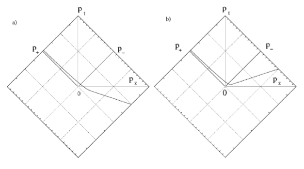
Figure 1: Plots of the $p_{-}>0$ dispersion relation for a) large $L\tilde{\mu}$ and b) small $L\tilde{\mu}$. Here $\epsilon=1$. The $p_{-}<0$ branches can be obtained by inverting these diagrams through the origin.

This verifies the claims made at the end of the previous subsection. Modulo our imprecision as to the boundary conditions, it would constitute a proof of stability if we could show that the modes labeled by the pair $(p_{z},n)$ formed a complete set of states on $\Sigma_{\epsilon}$, but this is beyond the scope of our work.

3.3 Quantum field theory

It was argued above that the classical field is in fact stable. Assuming that this is the case, we now show that no further difficulties arise when the field is quantized. In particular, we will assume below that there is a complete set of states labeled by real eigenvalues $p_{-}$. Much of this material has appeared before in [33, 14, 15], but we repeat it here for clarity and completeness.

It is convenient to drop the requirement of translation invariance in $x^{+}$ and to allow a general plane wave. Thus, in this subsection we require only that our field has an expansion of the form

$$\phi=\int dp_{-}d\alpha\ a_{p_{-},\alpha}\phi_{p_{-},\alpha},$$ (39)

where $p_{-}$ ranges over $(-\infty,+\infty)$ and $a_{p_{-},\alpha}$ is the requisite operator valued coefficient for the mode $\phi_{p_{-},\alpha}$. Again, the mode $\phi_{p_{-},\alpha}$ is an eigenstate of $\partial_{-}$ with eigenvalue $p_{-}$.

Some coefficients $a_{p_{-},\alpha}$ will be creation operators and some will be annihilation operators as determined by the commutation relations. As usual, these commutation relations may be computed from the Klein-Gordon inner products of the corresponding mode functions (see, e.g., [34]):

$$[a_{p_{-},\alpha},a_{\tilde{p}_{-}\alpha}]=-i(\phi_{p_{-},\alpha},\phi_{\tilde{p}_{-},\tilde{\alpha}})_{KG}=-i\int_{\Sigma}\phi_{p_{-},\alpha}\stackrel{{\scriptstyle\leftrightarrow}}{{\partial}}_{n}\phi_{\tilde{p}_{-},\tilde{\alpha}}\sqrt{g_{\Sigma}}d\Sigma.$$ (40)

Our convention is that the Klein-Gordon inner product is linear in both entries and that the inner product of real functions is real. In (40), $n$ is the unit normal vector to the Cauchy surface $\Sigma$ and $g_{\Sigma}$ is the determinant of the induced metric on $\Sigma$. Since the Klein-Gordon product is conserved, (40) may be evaluated on any Cauchy surface $\Sigma$.

It is well known that the treatment of plane wave backgrounds simplifies in a light cone formalism. This suggests that we take the surface $\Sigma$ to be of the form $x^{+}=constant$. However, there are several subtleties with this choice. The first is that, as noted above, such surfaces are not Cauchy surfaces. However the only causal curves which fail to cross such a surface are those that asymptotically have constant $x^{+}$. Such curves are a set of measure zero. In particular, each null geodesic crosses $\Sigma$ exactly once unless it lies along an orbit of $\frac{\partial}{\partial x^{-}}$ (see, e.g., section 2.2).

The other two issues are of a more direct practical sort. Since a surface with $x^{+}=constant$ is null, the normal cannot be normalized and the induced measure vanishes. However, these problems cancel against each other as $d\Sigma\sqrt{g_{\Sigma}}\partial_{n}$ has a well-defined limit when $\Sigma$ is approximated by a family of spacelike surfaces $\Sigma_{\lambda}$. We choose $\Sigma_{\lambda}$ to be defined by $x^{+}=f_{\lambda}(x^{-},x^{i})$ for, e.g.,

$$f_{\lambda}=\frac{\tanh(x^{-}/\lambda)}{1+\lambda^{-2}(x^{i}\mu^{2}_{ij}x^{j})^{2}}.$$ (41)

It is not hard to show that $\Sigma_{\lambda}$ is spacelike for sufficiently large $\lambda$, and that the family converges to the surface $x^{+}=0$.

A straightforward calculation shows that in this limit we have $\sqrt{g_{\Sigma}}\sim\lambda^{-1/2}$, while $\partial_{n}\sim\lambda^{1/2}\partial_{-}$ and $d\Sigma\sqrt{g_{\Sigma}}\partial_{n}$ asymptotes to a constant times $dx^{-}d^{8}x\partial_{-}$. As a result, the Klein-Gordon inner product on $\Sigma$ takes the form

$$(\phi_{p_{-},\alpha},\phi_{\tilde{p}_{-},\tilde{\alpha}})_{KG}=A\int_{\Sigma}\phi_{p_{-},\alpha}\stackrel{{\scriptstyle\leftrightarrow}}{{\partial}}_{-}\phi_{\tilde{p}_{-},\tilde{\alpha}}dx^{-}d^{8}x.$$ (42)

where $A$ is a positive normalization coefficient.

Thus, the Klein-Gordon inner product will be proportional to $p_{-}$, and $p_{-}$ will determine the all important sign of the commutation relations. Let us make the following standard choices for the mode functions $\phi_{p_{-},\alpha}$. First, we take modes with opposite $p_{-}$ and the same $\alpha$ to be complex conjugates, $\phi_{-p_{-},\alpha}=\overline{\phi_{p_{-},\alpha}}$. Second, we take modes with distinct $\alpha$ to be orthogonal in $L^{2}({\bf R^{8}},d^{8}x)$. Finally, taking the normalization of our modes to be $1/\sqrt{A|p_{-}|}$ in $L^{2}({\bf R^{9}},d^{8}xdx^{-})$, we find that the Klein-Gordon inner product for modes with $p_{-}>0$ yields:

$$[a_{p_{-},\alpha},a_{\tilde{p}_{-}\alpha}]=\rm{sign}(p_{-})\delta(p_{-}+\tilde{p}_{-})\delta(\alpha,\tilde{\alpha}).$$ (43)

This is the characteristic algebra of creation and annihilation operators. Note that the reality of $p_{-}$ was critical in writing $p_{-}/|p_{-}|=\rm{sign}(p_{-})$.

From (43) we see that $a_{p_{-},\alpha}$ is an annihilation operator for $p_{-}>0$ and a creation operator for $p_{-}<0.$ The details of modes with $p_{-}=0$ exactly are a mere matter of convention since there are no normalizable $p_{-}=0$ modes. Note that when an eigenvalue of $\mu^{2}$ is negative, the spectrum of $[4\delta^{ij}\partial_{i}\partial_{j}-(x^{i}\mu^{2}_{ij}x^{j})p_{-}^{2}]$ covers the entire real line so that negative values of $p_{+}$ can arise for any $p_{-}$ and, in particular, mode functions associated with creation operators can have either sign of $p_{+}$. In this sense we will necessarily have negative energy particles. However, we repeat that $p_{+}$ always remains real so that the modes of $\phi$ are stable. The structure of the Fock space is much like that of a massless free field in Minkowski space. In particular, the vacuum is the unique normalizable state with $p_{-}=0$. This rules out any pair creation of particles from the vacuum so that the vacuum is stable. Since the theory is non-interacting, each $n$-particle state is stable as well.

3.4 Interactions in Quantum field theory

Suppose, however, that we now turn on some self-interaction for our massive field. The vacuum must remain stable for the reason stated in section 3.3 above: it is the only normalizable state with $p_{-}=0$. However, a discussion of the particle states is more interesting.

In Minkowski space, any massless particle remains stable because energy-momentum conservation forbids its decay. But energy-momentum conservation in our background is more subtle. While each surface of constant $x^{+}$ is homogeneous, the generators of those translations do not commute with $\partial_{+}$. In particular, the momenta $p_{i}=-i\frac{\partial}{\partial x^{i}}$ corresponding to simple translations in $x^{i}$ do not generate symmetries and are not conserved.

This breaking of translation invariance should in general allow any one-particle state to decay. This is not particularly remarkable in the time-dependent case, as a time dependent background can be thought of as containing propagating waves with which our particle can interact. Let us therefore concentrate on the time independent case where $\mu^{2}_{ij}$ is constant.

To orient ourselves we begin by considering those $\mu^{2}_{ij}$ which are positive definite. Here the momenta $p_{\pm}$ are positive and $p_{+}$ has a discrete spectrum. In fact, the mode with lowest $p_{+}$ has $p_{+}>0$. As a result, a particle in this lowest mode $p_{+}$ is again clearly stable by conservation of $p_{+}$. This is also true of strings in the maximally supersymmetric plane wave [11].

In contrast, when $\mu_{ij}^{2}$ has a negative eigenvalue, the spectrum of $p_{+}$ is unbounded below and energy-momentum conservation allows any particle to decay. Furthermore, any decay products will be dispersed by the repulsive tidal forces removing any hope of stability being restored by interactions among these products. It is clear that an infinite number of particles will be created as $x^{+}\rightarrow\infty$. As a result, the S-matrix will be non-unitary and the usual scattering theory to be inappropriate. However, there remains the possibility of the existence of a self-adjoint Hamiltonian which implements unitary time evolution or some other well-defined notion of time evolution over finite periods of time. We argue that this is the case in two ways: first by imposing an infra-red cut-off, and second by analogy with a more familiar system with similar properties.

1. One can impose an infra-red cut-off by placing the system in a box. This makes the spectrum of $p_{+}$ both bounded below and discrete. As a result, the lowest one-particle states are stable. Since the infra-red regulated theory is sufficient to describe the local dynamics of the full theory within small regions of spacetime, this local dynamics is well-defined.

2. A useful analogy can be constructed by making use of the observation that our Fock space resembles that of a massless field in Minkowski space. In that case, for any interaction, one-particle states are prevented from decay by energy-momentum conservation. But suppose that we break translation invariance by adding a localized potential (a ‘scattering center’) near the origin. The scattering center can remove excess momentum so that a massless particle is now allowed to decay. Note that massless particles away from the scattering center are stable, so the theory remains unitary for any finite number of scattering centers. However, if we construct an infinite lattice of scattering centers, then the decay process can continue ad infinitum and one expects the theory to become non-unitary. Nonetheless, the theory is locally equivalent to the earlier example with a single scattering center. Thus the model is well-defined as a local quantum field theory.

In fact, non-unitarity due to infra-red divergences is common place even in free quantum field theory on non-compact spaces. For example, this feature arises whenever the background is both time dependent and spatially homogeneous with non-compact spatial slices. The time dependence leads to particle creation, which by translation invariance must yield some finite particle number per unit volume. Since space is infinite in volume, the total particle number diverges and the evolution is non-unitary. This is one reason why quantum field theory in general curved backgrounds is often discussed in terms of algebraic local quantum field theory (see, e.g., [35]). Note that this sort of non-unitary has nothing to do with the black hole ‘information loss paradox’.

One may ask what are the physical effects of the infinite decay of particles in the plane wave background. For example, does it lead to a large back-reaction on the background spacetime?  In the limit of weak coupling, the production rate must be slow. Thus, we expect that, for weak coupling and if considered for a short time, the particle production instability does not lead to a large back-reaction. It seems clear that, although scattering theory may not be applicable, there is no reason to regard our spacetime as leading to an ill-defined quantum field theory.

4 String theory in the plane-wave background

Since our initial motivation for studying plane waves was their importance as exactly solvable string backgrounds, it is important to ask how stringy effects modify the quantum field theoretic picture described above. Of particular concern is the fact that the eigenvalues of $\mu^{2}_{ij}$ are often described as leading to mass terms in the string sigma model, so that one might expect negative eigenvalues to lead to tachyons and instabilities. We shall argue this is not the case, though some interesting behavior does result.

We begin by briefly reviewing the quantization of the string in an arbitrary time-independent plane wave background. We use the Brinkmann coordinates $x^{\mu}$ (so that the spacetime metric again takes the form 1) and choose worldsheet coordinates ($\tau,\sigma$) with $\tau$ an (as yet unknown) function of $x^{+}$, and $\sigma$ an orthogonal spacelike coordinate normalized to have period $2\pi$. The remaining gauge freedom is fixed by requiring the worldsheet metric to be conformal to the Minkowski metric. The function $\tau(x^{+})$ is then determined by the equations of motion.

Varying the sigma-model action with respect to $x^{-}$ leads to the equation

$$(-\partial_{\tau}^{2}+\partial_{\sigma}^{2})x^{+}=0.$$ (44)

Note that the only solutions consistent with the gauge fixing specified above are $x^{+}(\tau)=-\frac{1}{2}p_{-}\tau+x^{+}(0)$ for some constants $p_{-}$ and $x^{+}(0)$.

For simplicity, let us assume that the matrix $\mu^{2}_{ij}$ is diagonal, with eigenvalues $\mu^{2}_{i}$. The equation of motion for a transverse coordinate $x^{i}$ is then

$$(-\partial_{\tau}^{2}+\partial_{\sigma^{-}}^{2})x^{i}-\frac{1}{4}p_{-}^{2}\mu^{2}_{i}x^{i}=0,$$ (45)

so that the eigenvalue $\mu^{2}_{i}$ contributes a squared-mass to the field $x^{i}$. While $\mu^{2}_{i}$ itself can be rescaled by rescaling $x^{+}$ and $x^{-}$, the factor of $p_{-}^{2}$ scales in the opposite way so that $p_{-}^{2}\mu^{2}_{i}$ is invariant under this transformation.

As usual, it is beneficial to decompose the coordinates $x^{i}$ into modes. We refer to the mode of $x^{i}$ with $\sigma$-dependence $e^{im\sigma}$ as $x^{i}_{m}$. Taking the Fourier transform of equation (45) yields

$$\partial_{\tau}^{2}x^{i}_{m}=(m^{2}+\frac{1}{4}p_{-}^{2}\mu^{2}_{i})x^{i}_{m},$$ (46)

so that the mode is stable for $m^{2}+\frac{1}{4}p_{-}^{2}\mu_{i}^{2}>0$ and unstable for $m^{2}+\frac{1}{4}p_{-}^{2}\mu_{i}^{2}<0$. In the latter case, gravitational tidal forces cause the string to stretch indefinitely in the $x^{i}$ direction.

Due to the compactness of the string, it is clear that only a finite number of modes will be unstable for any given values of $p_{-}$, $\mu^{2}_{i}<0$. Suppose first that $0>\frac{1}{4}p_{-}^{2}\mu^{2}_{i}>-1$, which, roughly speaking, is the case where the spacetime curvature is much less than string scale in the reference frame of the string. Since only the zero mode is unstable, the string has no problem retaining its integrity. The only instability is that the center of mass of the string is rapidly pushed away from $x^{i}=0$. One expects that the string spectrum will be discrete, and that different internal excitations can be interpreted as particles corresponding to different quantum fields. The stability of such fields has already been discussed in section 3.

More generally, we may work out the canonical momenta to find that the squared masses of string states are given by

$$M^{2}=p_{\alpha}p_{\beta}g^{\alpha\beta}=\sum_{m\geq 0}\frac{1}{4}p_{-}^{2}[\overline{x}^{i}_{m}\mu_{ij}^{2}x^{j}_{m}]+\sum_{m>0}\big{(}\overline{p}_{m}^{i}\delta_{ij}p_{m}^{j}+m^{2}\overline{x}^{i}_{m}\delta_{ij}x^{j}_{m}\big{)},$$ (47)

where $\overline{x}^{i}_{m}$ represents the complex conjugate of $x^{i}_{m}.$ Similarly, the dispersion relation takes the form

$$p_{+}p_{-}=\sum_{m\geq 0}\big{(}\frac{1}{4}p_{-}^{2}[\overline{x}^{i}_{m}\mu_{ij}^{2}x^{j}_{m}]+\overline{p}_{m}^{i}\delta_{ij}p_{m}^{j}+m^{2}\overline{x}^{i}_{m}\delta_{ij}x^{j}_{m}\big{)},$$ (48)

One sees that the right hand side of either (47) or (48) can easily be negative. However, this occurs only at large $p_{-}$. The dispersion relation is qualitatively of the same form as that in section 3, where we saw that it did not in fact lead to instabilities. Note that while there is now a new conceptual point associated with the fact that the locally measured $M^{2}$ is a function of momentum (whereas in section 3 $g^{\alpha\beta}p_{\alpha}p_{\beta}$ was constant), this does not in any way effect the analysis of the dispersion relation (48).

As a result, the arguments given in section 3 apply here as well. Said differently, while there are clearly particle instabilities in which the strings are infinitely stretched or pushed off to infinity, there appear to be no field theoretic instabilities in which small field perturbations grow exponentially in $x^{+}$.

However, an interesting phenomenon arises when one investigates the low energy effective description of strings in this background. One might expect that a low energy limit could be obtained by restricting the light cone energy ($p_{+}$) to be small. However, since negative $p_{+}$ states exist, interactions will generate particles with arbitrarily large $p_{+}$ even when the total value of $p_{+}$ is small. The same is true if we attempt to restrict to small $p_{t}$ for for any $t$ associated with one of the cut-off ‘Cauchy surfaces’ $\Sigma_{\epsilon}$ of section 3.1. In contrast, we have seen that $p_{-}$ is positive for all particles, so that it makes sense to restrict to small $p_{-}$. While only a finite number of fields can then reach negative $p_{+}$, the associated low energy theory nevertheless contains an infinite number of fields.

For completeness, let us briefly discuss the fermionic sector. Following [6, 7, 37] the fermionic part of the string action can be written in terms of the pull back to the world sheet of the covariant derivative entering in the variation of the gravitino:

$$D_{a}=\partial_{a}+{1\over 4}\partial_{a}x^{m}\big{[}\ (\omega_{\mu\nu m}-{1\over 2}H_{\mu\nu m}\rho_{3})\Gamma^{\mu\nu}+({1\over 3!}F_{\mu\nu\lambda}\Gamma^{\mu\nu\lambda}\rho_{1}+{1\over 2\cdot 5!}F_{\mu\nu\lambda\rho\kappa}\Gamma^{\mu\nu\lambda\rho\kappa}\rho_{0})\Gamma_{m}\ \big{]}$$ (49)

where the $\rho_{s}$-matrices in the $I,J$ space are the Pauli matrices $\rho_{1}=\sigma_{1}$, $\rho_{0}=i\sigma_{2}$. The action becomes

$${\cal L}=i(\eta^{ab}\delta_{IJ}-\epsilon^{ab}(\rho_{3})_{IJ})\partial_{a}x^{m}\bar{\theta}^{I}\Gamma_{m}D_{b}\theta^{J}$$ (50)

Here $\theta^{I}$ ($I$=1,2) are the two real positive chirality 10-d MW spinors and $\rho_{3}=$diag(1,-1). Thus the masses of the fermions are completely determined by the value of the RR form fields. In the simplest case of a background with only the 5-form field strength non-vanishing $F_{5}=f(x^{+})dx^{+}\wedge(\omega_{4}+*\omega_{4})$, the only nontrivial Einstein equation of motion is $\rm{Tr}\,\mu_{ij}^{2}=[f(x^{+})]^{2}$ which does not directly feel the effect of one negative eigenvalue in $\mu_{ij}^{2}$. Thus, one may easily deform, for example, the BFHP plane wave to one with a negative eigenvalue without changing the behavior of worldsheet Fermions. As a result, at least for appropriate choices of Ramond-Ramond fields, consideration of Fermions adds nothing new to the picture discussed above.

5 Discussion

In this work we have analyzed the singularity structure of plane wave metrics and provided a simple criterion to determine the presence of singularities. In section 2 we have also presented careful analysis of the Penrose limit of an AdS background dual to a gauge theory having a mass scale. Our analysis provides a strictly gravitational approach to this problem. We have discussed the stability of classical and quantum fields in backgrounds having at least one negative eigenvalue of the matrix $\mu^{2}_{ij}$. We have found by the introduction of an infrared regulator that the obvious candidate modes for instabilities are in fact stable. While we have given only the most cursory treatment of boundary conditions, some justification that this is sufficient was given based on the analyses of plane wave asymptotic structures presented in [31, 30].

We have also discussed certain features of string theory in plane waves with negative eigenvalues. Again, the theory appears to be stable, though any low energy description necessarily involves an infinite number of fields.

We have not yet considered the implications of string interactions. Let us take a moment to do so now. Such interactions trigger an instability of one-particle states in parallel with that discussed in section 3.4 and the resulting S-matrix will be non-unitary. As in the field theoretic case, the issue might be resolved through a more local treatment. However, it is an open question to what extent string theory may be formulated locally and the difficulties of, for example, using a string field approach to closed strings are well known.

One difference between the string and field theoretic cases is the large number of stringy negative energy states that exist at large $p_{-}$. As we have seen, imposing a strict infra-red cutoff on $x^{i}$ and an ultra-violet cutoff on $p_{-}$ discards most of these states and truncates the system to having only a finite number of negative energy fields. However, as this cut-off is taken to infinity the number of negative energy fields grows exponentially. One expects this to have important effects, at the very least on the thermodynamics of the system. More fundamentally, it raises the possibility that non-locality at the string scale could interact with these negative energy states in a disastrous fashion.

On the other hand, it is also possible that string interactions act to limit the instability discussed above. Most of the negative energy modes require large $p_{-}$ but, since $p_{-}$ is positive and conserved, finite coupling will induce strings with large $p_{-}$ to decay into states with small $p_{-}$; i.e., into strings which are more stable. It would therefore be interesting to understand a strong coupling description of this effect.

There are thus many interesting and fundamental issues raised by string interactions in negative eigenvalue plane wave backgrounds. A proper analysis would seem to require several new techniques, possibly in a string field theoretic setting. We hope that the questions raised by these solvable backgrounds will spur the development of such techniques.

In most of this work we have assumed that at least one eigenvalue of $\mu^{2}_{ij}$ is negative and that at least one is positive. Let us now briefly address the case where all the eigenvalues of the matrix $\mu_{ij}^{2}$ are negative. This case in unphysical if (1) is the Einstein metric since it violates the weak null energy condition. However, it may well arise in the string metric (see, e.g. [13]) when the dilaton depends on $x^{+}$. To analyze the stability of this metric we note that an explicit coordinate transformation is known [30] that maps this space conformally into a slice of Minkowski space. Here, boundary conditions are readily studied and the results proceed in parallel with those found above. If desired, this spacetime may again be conformally embedded into the Einstein static universe, though the resulting map is of very different nature than the associated conformal embedding of the BFHP plane wave.