Confining potential in a color dielectric medium with parallel domain walls

Abstract

We study quark confinement in a system of two parallel domain walls interpolating different color dielectric media. We use the phenomenological approach in which the confinement of quarks appears considering the QCD vacuum as a color dielectric medium. We explore this phenomenon in QCD₂, where the confinement of the color flux between the domain walls manifests, in a scenario where two 0-branes (representing external quark and antiquark) are connected by a QCD string. We obtain solutions of the equations of motion via first-order differential equations. We find a new color confining potential that increases monotonically with the distance between the domain walls.

I Introduction

The color dielectric models have been used to describe phenomenologically the confinement of quarks and gluons inside the hadrons — see Refs. fl ; mit ; slac ; cornell for pioneering papers on this subject. We shall investigate the quark confinement in a system of two parallel domain walls separating different color dielectric media. Such a system is regarded as a hadron and our main goal in this paper is to search for a confining potential of the color electric field. The color dielectric effect is achieved via coupling between a color dielectric function $G$ chosen properly and the dynamical term of the gauge field. As one knows the color vacuum in QCD has an analog in QED. In QED the screening effect creates an effective electric charge that increases when the distance between a pair of electron-antielectron decreases. On the other hand, in QCD there exists an anti-screening effect that creates an effective color charge which decreases when the distance between a pair of quark-antiquark decreases. This means that for small distance (large momentum transfer) the quarks and gluons are considered approximately free inside the hadrons (asymptotic freedom).

In the examples described above, the screening effect is essentially due to the vacuum polarization in the relativistic limit. However, it is believed to be possible to treat the physics of quarks quite well in non-relativistic models of hadrons. This is of special interest in physics of heavy quarks, where one considers non-relativistic quarks and antiquarks connected by a color flux tube known as a QCD string. The energy of such configuration is described by confining potentials, i.e., by potentials that increase linearly with the distance. In color dielectric models one considers the QCD vacuum as a color dielectric medium. This is somehow analog to what happens with two electrical charges of opposite signs embedded in a polarizable dielectric medium. This is a common phenomenon that occurs in classic electrodynamics. The Lagrangian should contain a term like $G\,F_{\mu\nu}F^{\mu\nu}$ in order to describe the dielectric effects on the electric field, e.g., the displacement vector. The dielectric function $G(r)$ usually assumes the behavior: $G(r\!\gg\!d)\!\geq\!1$ and $G(r\!\ll\!d)\!<\!1$, where $d$ is the diameter of the polarized molecules and $r$ represents an arbitrary position on the dielectric medium. The QCD analog to this electric effect is achieved using in the QCD Lagrangian the term $G\,F^{a}_{\mu\nu}F_{a}^{\mu\nu}$. The color dielectric function $G(r)$ in order to guarantee absolute color confinement must assume the behavior: $G(r\!>\!R)\!=\!0$ in the color dielectric medium (outside the hadron) and $G(r\!<\!R)\!=\!1$ inside the hadron, where $R$ is the radius of the hadron.

For simplicity, in this paper we focus attention on QCD in two-dimensions, QCD₂, for short. Two-dimensional QCD in the large $N_{c}$ limit was introduced long ago thooft74 . It is a truly relativistic field theory resembling the realistic four dimensional QCD — see, for instance, nefediev . The theory naturally exhibits confinement since the Coulomb force is confining in two dimensions.

We choose a function $W(\phi,\chi)$ for the self-interacting part of the real scalar fields $\phi$ and $\chi$. The function $W(\phi,\chi)$ is chosen such that one of the scalar fields provides kink (anti-kink) solutions and the other scalar field contributes to the color dielectric function $G(\phi,\chi)$, with the right behavior for confinement. We find a solution representing two parallel domain walls that confine the color flux in between the two walls. In $(3,1)$ dimensions, the kink solutions are seen as thick domain walls which in the thin limit are regarded as 2-branes that can be found in string/M-theory. In the QCD realm, a 2-brane solution can be a place where the color flux terminates. This possibility has been considered first in the context of M-theory witten97 and also in field theory trodden ; campos ; shifman ; dvali ; sakai . In this scenario one considers a QCD string (flux tube) ending on a 2-brane (quark or antiquark). The QCD string itself is usually good to describe the spectra of heavy mesons such as charmonium or bottomonium — see td ; wil . Since we shall restrict ourselves to a two-dimensional theory, our kink (anti-kink) solutions will be regarded as 0-branes (quark or antiquark), which are the ending points for the QCD₂ string (flux line). In our model the two parallel domain walls solution (0-branes) that confines the color field can be regarded as a QCD₂ string connecting a quark to an antiquark.

In order to find classical solutions of the equations of motion we take advantage of the first-order differential equations that appear in a way similar to the Bogomol’nyi approach, although we are not dealing with supersymmetry in this paper. The formalism lead us to a suitable potential $V$ in order to make applications feasible. The first-order equations for the scalar fields decouple from the gauge field part. The dynamics of the fermionic sector, used to describe quarks is not considered at this stage of the calculations. Rather we regard the fermionic (quarks) effects via an external color current source. We also assume that the set of QCD₂ equations of motions can be replaced to another set, which consider only Abelian fields. This is because through the color dielectric function $G(\phi,\chi)$ the scalar field couples to an average of the gauge field $A^{a}_{\mu}$ NPA448 . Thus, it suffices to consider only the Abelian part of the non-Abelian gauge dynamics.

We organize this work as follows. In Sec. II we introduce the Lagrangian of the QCD₂ in a color dielectric medium and then we solve the equations of motion using first-order differential equations. The parallel domain wall solution that we find allows to have a confining color electric potential. In Sec. III we comment the results. Our notation is standard, and we use dimensional units such that $\hbar\!=\!c\!=\!1$, and metric tensor with signature $(+,-)$.

II QCD₂ with color dielectric function

A general theory of QCD₂ in a color dielectric medium can be described by the Lagrangian

$${\cal L}^{2} = -\frac{1}{4}G(\phi,\chi)F^{a}_{\mu\nu}(x)F_{a}^{\mu\nu}(x)$$ (1)

$$+\frac{1}{2}\partial_{\mu}\phi(x)\,\partial^{\mu}\phi(x)+\frac{1}{2}\partial_{\mu}\chi(x)\,\partial^{\mu}\chi(x)-V(\phi,\chi)$$

$$+{\bar{\psi}}(x)(\,i\,\gamma^{\mu}\partial_{\mu}-m)\psi(x)$$

$$+{\bar{\psi}}(x)(g\gamma^{\mu}A^{a}_{\mu}X_{a}-f(\phi,\chi)\,)\psi(x)$$

where $X_{a}$ are $SU(N_{c})$ color matrices, $F^{a}_{\mu\nu}\!=\!\partial_{\mu}A^{a}_{\nu}-\partial_{\nu}A^{a}_{\mu}+g\,f^{a}_{bc}A^{b}_{\mu}A^{c}_{\nu}$, $x$ stands for $(x_{0},x)$ and we have suppressed the flavor indices. The quark spinor field $\psi$ is in general coupled to the scalar fields via the Yukawa coupling term ${\bar{\psi}}f(\phi,\chi){\psi}$. Here, however, we first discard all the fermions, to focus on the bosonic background fields. The presence of fermions will be further examined below, to discuss how the walls can be charged.

In a medium which accounts mainly for one-gluon exchange, the gluon field equations linearize and are formally identical to the Maxwell equations wil . In this sense, it suffices to consider only the Abelian part of the non-Abelian strength field NPA448 , i.e., $F^{a}_{\mu\nu}\!=\!\partial_{\mu}A^{a}_{\nu}-\partial_{\nu}A^{a}_{\mu}$. Further, without loss of generality we can suppress the color index $``a"$ if we take an Abelian external color source slusa due to quarks or antiquarks represented by an external color current density $j^{\mu}_{a}$. This is because the results both for Abelian and non-Abelian cases are very similar slusa ; dick1 ; dick2 ; cha1 ; cha2 . We account for all these facts, thus the model we start with to investigate confinement is the effectively Abelian Lagrangian

$${\cal L}^{2}_{eff}\! = \!-\frac{1}{4}G(\phi,\chi)F_{\mu\nu}F^{\mu\nu}+j_{\mu}A^{\mu}$$ (2)

$$+ \frac{1}{2}\partial_{\mu}\phi\,\partial^{\mu}\phi+\frac{1}{2}\partial_{\mu}\chi\,\partial^{\mu}\chi-V$$

where $j_{\mu}$ is an Abelian external current density.

II.1 Equations of motion

We search for static solutions of the equations of motion. Thus, we consider the fields depending only on the spatial coordinate, $x$. The equations of motion that follow from (2) are written as

$$\frac{d^{2}\phi}{dx^{2}} = V_{\phi}-\frac{1}{2}\,G_{\phi}\left(\frac{dU}{dx}\right)^{2}$$ (3)

$$\frac{d^{2}\chi}{dx^{2}} = V_{\chi}-\frac{1}{2}\,G_{\chi}\left(\frac{dU}{dx}\right)^{2}$$ (4)

and

$$\frac{d}{dx}\left[G(\phi,\chi)\frac{dU}{dx}\right]=\rho(x)$$ (5)

where we have set $U\!=\!A^{0}$ and $\rho\!=\!j^{0}$. Also, $V_{\phi}$ and $G_{\phi}$ stand for derivatives with respect to $\phi$, and so forth. Now, we choose the potential in the form

$$V(\phi,\chi,x)=\frac{1}{2}W^{2}_{\phi}+\frac{1}{2}W^{2}_{\chi}-\frac{1}{2G}\left[\int^{x}dx^{\prime}\,\rho(x^{\prime})\right]^{2}$$ (6)

where the function $W(\phi,\chi)$ is smooth everywhere, in general. The form of $V(\phi,\chi,x)$ in (6) appears because we want to use first-order differential equations, instead of the second-order equations of motion. To see this, we notice that the above equations of motion are solved by $\phi(x),\,\chi(x)$, and $U(x)$ that solve the new set of first-order equations

$$\frac{d\phi}{dx} = W_{\phi}$$ (7)

$$\frac{d\chi}{dx} = W_{\chi}$$ (8)

$$G(\phi,\chi)\frac{dU}{dx} = \int^{x}dx^{\prime}\,\rho(x^{\prime})$$ (9)

This result is inspired in the procedure introduced in Ref. bog , although here the situation is quite different because we are not minimizing the total energy of the system – see, for instance, Ref. bb2000 for further details. However, we can show that the above first-order equations solve the equations of motion.

To solve the first-order equations we first notice that the equations (7) and (8) do not couple with the other equation (9). We take advantage of this and we define the function $W(\phi,\chi)$ to look for solutions of (7) and (8). We consider

$$W(\phi,\chi)=\lambda\,a^{2}\phi-\frac{\lambda}{3}\,\phi^{3}-\mu\,\phi\chi^{2}$$ (10)

where $\lambda,\mu$ and $a\!>\!0$ are real parameters. For this particular $W$, the dynamical system (7) and (8) has four singular points, given by $(\phi\!=\!\pm a,\chi\!=\!0)$ and $(\phi\!=\!0,\chi\!=\!\pm\sqrt{\lambda/\mu}\,a)$, for $\lambda/\mu>0$, which are interpolated by domain wall solutions bb2000 ; bsr ; brs ; bb ; shvol ; bbb . Before going into this, let us now specify the functions $\rho(x)$ and $G(\phi,\chi)$. Since we are representing here quarks and antiquarks as domain walls (0-branes) with non-zero width, the color charge density is not necessarily point-like. In this way we introduce the color charge distribution on the walls as

$$\rho(x\pm s)=q\frac{\eta}{2}\,{\rm sech}^{2}\eta(x\pm s)$$ (11)

where $s$ is the center of the distribution, which we choose to be real and positive. This charge density is interesting since it tends to be point-like $[q\delta(x\pm s)]$ in the limit as $\eta\to\infty$. The point-like limit is realistic as long as $x\!\gg\!\Delta$, where the width $\Delta\!\sim\!1/\eta$ is of the same order as the quark (or antiquark) radius. As we show below, $\eta$ is defined according to the width of the domain wall solutions that solve (7) and (8).

Let us now discuss the choice (11) that we have just done for the color charge density on the walls. It can be justified due to the presence of fermion zero modes on the walls. To show this explicitly, we consider the Lagrangian density ${\cal L}^{\prime}\!=\!{\cal L}^{\prime}_{eff}+{\cal L}_{D}+{\cal L}_{Y}$, where ${\cal L}^{\prime}_{eff}$ is given in (2), with $j_{\mu}\!=\!q\bar{\psi}\gamma_{\mu}\psi$. The other fermion contributions are given by the Dirac Lagrangian density ${\cal L}_{D}$ and the Yukawa coupling term ${\cal L}_{Y}$. The variation $\delta{\cal L}^{\prime}/\delta\bar{\psi}=0$ gives the fermion equation of motion

$$i\gamma^{\mu}\partial_{\mu}\psi+q\gamma^{\mu}A_{\mu}\psi-[m+f(\phi,\chi)]\psi=0.$$ (12)

We choose $f(\phi,\chi)\!=-m+k\Phi(x)\!$, with $\Phi(x)\!=\!\phi(x)-\phi_{0}$ where $\phi(x)$ is the bosonic background solution for the scalar field $\phi$, which is given below, in Eq. (21). The meaning of $\phi_{0}$ is going to be clear later. Looking for two-dimensional solutions ($\mu\!=\!t,x$) we start with the Ansatz

$$\psi=e^{iqA_{0}(x)t}h(x)\epsilon_{\pm}$$ (13)

where $\epsilon_{\pm}$ is a constant spinor and $A_{0}(x)$ is the color electric potential. Substituting (13) in (12) and using the fact that $\gamma^{x}\epsilon_{\pm}=\pm i\epsilon_{\pm}$, we find the solution $h(x)\!=\!C\,\exp{[-iqA_{0}(x)t]}\times\exp{[\mp k\int^{x}\Phi(x^{\prime})dx^{\prime}]}$, where $C$ is an arbitrary constant. Now we use Eq. (13) to get to the spinor solution

$$\psi(x)=\Big{[}C\,e^{\mp k\int^{x}\Phi(x^{\prime})dx^{\prime}}\Big{]}\epsilon_{\pm}$$ (14)

The solution (21) [together with (22)] represent two parallel domain walls. Each domain wall can be treated separately. Explicitly, this can be done by shifting $x$ in (21) as $x\to\pm s+2z$ such that one has

$$\Phi(z)=\frac{a}{2}\Big{[}\tanh{\frac{2(z\pm s)}{\Delta}}+\tanh{\frac{2z}{\Delta}}\Big{]}-\phi_{0}.$$ (15)

Now it is clear that $\phi_{0}$ must be $(a/2)\tanh{({2z}/\Delta)}$ such that we are able to study each domain wall isolated which are described as

$$\Phi(z)=\frac{a}{2}\tanh{\frac{2(z\pm s)}{\Delta}}.$$ (16)

Note that, locally, each domain wall solution (16) changes its sign in $z\!=\!-s$ and $z\!=\!s$. Thus, there are fermion zero modes jack localized on the domain walls at the points $x\!=\!\pm s$. In fact, we can find the zero mode solutions explicitly: substituting (16) in (14) and integrating in $x^{\prime}\,\!(=\!z)$ we find the normalizable chiral zero modes

$$\psi=C\,{\rm sech}{\frac{2(x\pm s)}{\Delta}}\epsilon_{\pm}$$ (17)

where we have set $k=4/a\Delta$. With these solutions, the localized charge on the domain walls due to fermionic charge carriers is given by using the current density $j_{\mu}\!=\!q\bar{\psi}\gamma_{\mu}\psi$. The charge density is $\rho\!=\!j_{0}\!=\!q\psi^{\dagger}\psi$ and so, we use the fermion solutions (17) to find $\rho(x\pm s)=q(\eta/2)\,{\rm sech}^{2}{\eta(x\pm s)}$, where we have identified $\eta\!=\!2/\Delta$ and $\eta/2=C^{2}R$, with $R\!=\!\epsilon^{\dagger}_{\pm}\epsilon_{\pm}$ being a constant number. This charge distribution is the charge distribution that we have chosen in Eq. (11).

On the other hand, we define the color dielectric function as

$$G(\phi,\chi)=A\,\chi^{2}$$ (18)

where $A$ is a normalization constant, dimensionless. As we show below, this definition is sufficient to produce an absolute color confining effect since the $\chi^{2}$ solution has the appropriate behavior, to make the above $G$ to have the required asymptotic profile, as we have mentioned in the introduction.

We notice that the limit $\mu\to 0$ decouples the scalar fields, making the model meaningless. Also, the choice (10) appears as a simple extension of the $\phi^{4}$ model (with spontaneous symmetry breaking) to include another field, the $\chi$ field, which interacts with the gauge field via the color dielectric model that we propose, inspired in the former Refs. wil ; slusa ; dick1 ; dick2 .

II.2 Confinement with two parallel domain walls

Among several domain wall solutions connecting the four singular points of the system (7) and (8), when $W(\phi,\chi)$ is given as in Eq. (10), there is a particular solution of interest here: the two parallel domain wall solution reported in Refs. shvol ; volosh ; gani . To see this explicitly, we substitute (10) into the first-order equations (7) and (8) to obtain

$$\frac{d\phi}{dx} = \lambda(a^{2}-\phi^{2})-\mu\chi^{2}$$ (19)

$$\frac{d\chi}{dx} = -2\mu\phi\chi$$ (20)

This system presents analytical solutions such as

$$\phi = \frac{a}{2}\left[\tanh{\frac{\lambda a(x+s)}{2}}+\tanh{\frac{\lambda a(x-s)}{2}}\right]$$ (21)

$$\chi = \pm\sqrt{2}\,a\left[1-\tanh{\frac{\lambda a(x+s)}{2}}\tanh{\frac{\lambda a(x-s)}{2}}\right]^{1/2}$$ (22)

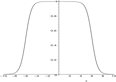
if one sets $\mu\!=\!\lambda/4$. This solution clearly represents two parallel domain walls at the positions $x\!=\!-s$ and $x\!=\!s$. It provides a color dielectric function $G=A\,\chi^{2}$ (with $A\!=\!1/2a^{2}$) with the proper behavior inside and outside the region in between the domain walls: $G\!\to\!1$ for $-s\!\leq x\!\leq\!s$, and $G\!\to\!0$ for $x\!>\!s,\,x\!<\!-s$, as we illustrate in Fig. 1. This characterizes an absolute color confinement, as desired. The interpretation of this is that the color flux inside such a region connects charged domain walls with opposite color charges.

Figure 1: The color dielectric function behavior is plotted in arbitrary units. It shows that the color field is confined in between the two domain walls, which are centered at $x=\pm s=\pm 6$.

It is now clear that $\eta$ in the color charge density function (11) should agree with the domain walls width that appears in the solutions (21) and (22), i.e., $\eta\!=\!\lambda a/2$. Let us now write the equation (9), with $\rho(x)$ and $G(\phi,\chi)$ defined as in (11) and (18) respectively, in the form

$$\chi^{2}\,\frac{dU}{dx}=qa^{2}\left(\tanh{\frac{x+s}{\Delta}}-\tanh{\frac{x-s}{\Delta}}\right)$$ (23)

where we are using $\Delta=2/\lambda a$ to represent the width of each domain wall. This expression has to be integrated over the external color charge density of the quark-antiquark pair represented by the solution obtained in Eqs. (21) and (22). The convention is such that the lines of the color electric flux come from the domain wall on $x\!=\!-s$ (a quark) and end on the domain wall on $x\!=\!s$ (an antiquark).

We substitute the solution (22) into the equation (23) to perform the integration in the interval that goes from $-s-\Delta/2$ to $s+\Delta/2$, which is the region where the solutions (21) and (22) appreciably deviate from trivial vacuum states. The result is

$$U(s)=2\sigma\left(s+\frac{\Delta}{2}\right)\,\tanh(2s/\Delta)$$ (24)

where we are using $\sigma=q/2$, as the string tension of the string that connects the quark-antiquark pair. At large distance, for $s\!\gg\!\Delta$ we obtain

$$U(s)\approx\sigma\,\Delta+2\,\sigma s,$$ (25)

which nicely reproduces the well-known linear behavior in quark confinement This is the scenario we have in the thin-wall limit.

The above scenario is introduced to represent a meson. In the region outside the parallel domain walls (the vacuum) the field $\chi\!\to\!0$ and so does the color dielectric function $G$, whereas the field $\phi$ is non zero. This scalar field can be excited around its vacuum $\phi_{0}$. Such excitation can be identified with $glueballs$, i.e., pure gluonic hadrons surrounding the meson. In our model the glueball mass is given by $\partial^{2}V(\phi)/\partial\phi^{2}|_{\phi=\phi_{0}}$, where $V(\phi)\!=\!(1/2)[W_{\phi}^{2}+W_{\chi}^{2}]|_{\chi=0}$ with the $W(\phi,\chi)$ chosen as in (10), with $\mu=\lambda/4$. The glueball mass is then given by $m_{GB}^{2}\!=\!4\lambda^{2}a^{2}$. One can redefine some quantities in terms of the glueball mass; for instance, the scale of symmetry breaking can be given as $a^{2}\!=\!3m_{q}/m_{GB}$, once we are identifying $m_{q}\!=\!2\lambda a^{3}/3$ (the mass $m_{q}$ of each quark is identified with the tension of each isolated wall). For heavy quarks we have $m_{q}\!\gg\!m_{GB}$ and then $a^{2}\gg 1$. Since the wall width $\Delta$ is $(2/\lambda a)$ and so, for finite $\lambda$ the thin-wall limit is then ensured, in accordance with the previous results.

Let us now turn attention to the small distance ($s\!\ll\!\Delta$) behavior of our model. We cannot use the above result (24) to examine the small distance behavior of the potential. This limitation is to be expected, since at small distance the two walls overlap and change the scenario. To circumvent this issue we turn back to solutions (21) and (22), to see that the limit $s\ll\Delta$ leads to other solutions, as follows

$$\phi(x) \to \phi^{(0)}(x)=a\,\tanh{\left(\frac{x}{\Delta}\right)}$$ (26)

$$\chi(x) \to \chi^{(0)}(x)=\pm\sqrt{2}\,a\,{\rm sech}{\left(\frac{x}{\Delta}\right)}$$ (27)

The solutions $\phi^{(0)}$ and $\chi^{(0)}$ were first obtained in Ref. bsr ; they represent genuine two-field solutions, not two-wall solutions anymore. This represents the thick wall solution with internal structure brs ; bb . The fields $\phi$ and $\chi$ play another game now. The field $\phi$ is regarded to describe a “bag” mit ; slac filled with gluons which is represented by $\chi$. It is not difficult to see that in doing all the above calculations in order to obtain the color potential using the solutions (26) and (27) we end up with a new confining potential. The leading contribution that appear from the right hand side of Eq. (23) in the limit $s\!\ll\!\Delta$ vanishes, making the potential constant, describing absence of force in between the gluons inside the bag, in agreement with the asymptotic freedom behavior of QCD. The bag represents a purely gluonic hadron, i.e., a gluewall, in analogy to the three-dimensional glueball. Our understanding is that at very small distance the pair quark-antiquark annihilates, decaying into a colorless gluewall.

III Comments and conclusions

In this paper we have presented a scenario which can describe quark confinement via a monotonically increasing color electric potential. This is achieved by considering a color flux confined to a region in between two parallel domain walls. In two-dimensional QCD, the color flux is confined to a flux line ending on 0-branes. This is similar to QCD strings connecting 2-branes in string/M-theory witten97 . The color electric potential varies linearly with distance, in the large distance limit between the domain walls, in the thin-wall limit. On the other hand, at very small distance, our results predict that the pair quark-antiquark annihilates to form a colorless gluewall. This is the (analog of a) purely gluonic hadron described by a bag represented by a domain wall with internal structure.

Despite its simplicity, we see that our model presents a very reasonable description of quark confinement at relatively large distance. This result encourages us to investigate more realistic models, taking into account mainly the non-Abelian character of the color dielectric medium. Another line of investigation is directly related to the way we couple the gauge field to the scalar fields via the dielectric function $G(\phi,\chi)$. This coupling is somehow similar to the coupling that appears in Kaluza-Klein compactifications involving non-Abelian dick1 ; dick2 and Abelian mts gauge fields. In this sense, an issue to be pursued refers to the relation between the two scalar fields that appear in the present work, and the dilaton and moduli fields used in Ref. mts .