Cluster Transformation Coefficients for Structure and Dynamics Calculations in n-Particle Systems:
Atoms, Nuclei, and Quarks

Abstract

The structure and dynamics of an n-particle system are described with coupled nonlinear Heisenberg’s commutator equations where the nonlinear terms are generated by the two-body interaction that excites the reference vacuum via particle-particle and particle-hole excitations. Nonperturbative solutions of the system are obtained with the use of dynamic linearization approximation and cluster transformation coefficients. The dynamic linearization approximation converts the commutator chain into an eigenvalue problem. The cluster coefficients factorize the matrix elements of the (n)-particles or particle-hole systems in terms of the matrix elements of the (n-1)-systems coupled to a particle-particle, particle-hole, and hole-hole boson. Group properties of the particle-particle, particle-hole, and hole-hole permutation groups simplify the calculation of these coefficients. The particle-particle vacuum-excitations generate superconductive diagrams in the dynamics of 3-quarks systems. Applications of the model to fermionic and bosonic systems are discussed.

1 Introduction

In the Heisenberg’s picture the time evolution of a system of particles is described by a commutator equation which involves the n-body Hamiltonian and the creation operators of the n-body ground- and excited-modes. However, the excitations of the reference vacuum, resulting from the scattering of particles from the vacuum to higher states (the particle-hole and particle-particle excitations), are completely neglected in this formulation, namely, the time evolution of the n-body-modes is described by a linearized Equation of Motion (EOM) [1] which involves only valence particles. Recently the original Heisenberg formulation of the n-body-dynamics has been generalized within the framework of the Dynamic-Correlation Model (DCM) [2] for fermions, the Boson Dynamic-Correlation Model (BDCM) [3] for bosons, and the Superconductive Dynamic- Correlation Model (SDCM) which describes superconductive- and polarization-effects [4]. In these models, the inclusion of the structure and the dynamics of odd/even quasi-particles into the calculations of the excitations of the model-vacuum led to the modification of the formal strcture of the original Heisenberg’s commutator equation. The new dynamics system is characterized by a set of coupled commutator equations which involve simultaneously the excitations of the valence quasi-particles and the excitations of the Intrinsic-Supercunductive-Vacuum States (ISVSs) i.e.: mixed-mode states formed by coupling the valence quasi-particles to the excitations of the vacuum (particle-particle and particle-hole). As in Ref. [4], the resulting mixed-mode states are classified in terms of the following mixed-mode wave functions: (a) valence particles coupled to ISVSs formed by include particle-hole, particle-particle and hole-hole vacuum-excitation modes that have the same parity of the valence particles; (b) valence particles and ISVSs formed by exciting particle-hole, particle-particle and hole-hole having a parity different from that of the valence particles. The superconductive vacuum states (b) are not considered by perturbative theories, although they may be associated to the creation of virtual particles [2, 3] giving important contribution to dynamic theories. The superconductive vacuum excitation modes are important mainly at high densities [4], although the overlap of the particle-particle excitation modes may influence, due to the strong Pauli blocking effects in the ISVSs, the particle-hole excitation mechanism also at medium energies. In this paper we disregard the superconductive effects, which will be the subject of a paper in preparation, and discuss only the effect of the particle-hole excitation mechanism on ground state properties of atomic, nuclear, and quark systems. In principle, the system of commutator equations may be solved perturbatively by means of substitution method which consists in inserting the higher order commutators into the previous calculated commutators. However, such perturbative method is usually not convergent for systems of strong interacting particles and, therefore, will not be discussed here. We will study nonperturbative solutions based on the following: (a) a linearization ansatz motivated by the consideration that in the low energy domain only few particle excitations are energetically representative while the higher excitation modes (with admixture probability less than 0.1 %) may be omitted from the model space; (b) cluster transformation coefficients which provide an exact solution for the complex n-body matrix elements that are input of the commutator equations. The wave functions, solutions of the calculated collective eigenvalue equation are classified as in Refs. [2, 3] in terms of Configuration Mixing Wave Functions (CMWFs). In Section II, we calculate the commutator chain for one particle-, two particle-, and three particle- creation operators. The generalization of the model to hole- and (particle-hole)-valence operators is not given explicitly because of easy extrapolation from the present particle formulation. The commutator chain is then linearized and converted into an eigenvalue problem which is solved calculating the n-body matrix elements within the cluster transformation coefficients. In Section III, solutions of the nonlinear eigenvalue equation for one valence particle/hole are obtained and the HFS constants of hydrogen- and lithium-like heavy ions are calculated. In Section IV, the commutator chain is solved for two and three valence particles and the resulting CMWFs are used to calculate the matter distribution of halo nuclei. In Section V, an application to the three dressed quark systems is discussed in order to provide new theoretical data for the polarizability of the proton. For a measurement of the proton polarization, novel ultra/intense lasers may be useful, like the PHELIX-petawatt laser presently under construction at GSI, have to be used. A direct way for a precision measurement seems to be in reach by the latest improvements of energetic multi-MeV photon sources using laser backscattering at electron storage rings.

2 The nonlinear commutator chain

The nonlinear commutator chain is an extension of the Heisenberg’s equation. It allows us to address the situation where valence clusters and core clusters are almost energetically degenerated and may, therefore, coexist. We introduce valence systems formed of either neutrons or protons. and define the valence states as

$$\>\>|\Gamma_{J}(\{n\}~{}particles)\rangle\>=\sum_{\alpha_{n}}\>X^{(n)}_{\alpha_{n}J_{n}}\>N^{(n)}_{\alpha_{n}J_{n}}\>A^{\dagger}_{n}(\alpha_{n}J_{n};J)|0\rangle,$$ (1)

where $n=1,2,3$ and $J$ is the total spin. The $N^{(n)}_{\alpha_{n}J_{n}}$ are the normalization constants, $X^{(n)}_{\alpha_{n}J_{n}}$ the mode amplitudes, and $\alpha_{1}$ denotes the other quantum numbers of the valence particles. The creation operator is defined by

$$A^{\dagger}_{1}(\alpha_{1}j_{1};J)\equiv a^{\dagger}_{j_{1}}\,$$ (2)

for one valence particle (fermion);

$$A^{\dagger}_{2}(\alpha_{2}J;J)\equiv(a^{\dagger}_{j_{1}}\otimes a^{\dagger}_{j_{2}})^{J}\,$$ (3)

for one valence pair (boson);

$$A^{\dagger}_{3}(\alpha_{3}J_{1};J)\equiv((a^{\dagger}_{j_{1}}\otimes a^{\dagger}_{j_{2}})^{J_{1}}\otimes a^{\dagger}_{j_{3}})^{J}$$ (4)

for three valence particles (fermion). Hence, in Eq. (1), $J_{n}=j_{1}$ for one particle, $J_{n}=J$ for two particles, and $J_{n}=J_{1}$ for three particles.
In the literature, various approaches, as reported in Ref. [3], have been proposed for including core excitations. In Shell-Model calculations the residual interaction between the valence particles excites the valence pairs to higher single particle states, leaving the vacuum in the $J=0$ ground state. In Ref. [5] the core excitations have been included in the Shell-Model calculations through introducing the coupling between the valence particles and the collective $J=2^{+}$ core-excited states. In the DCM and BDCM the core excitation is included through coupling the valence fermionic/bosonic states, Eqs. (2, 3) to intrinsic bosonic states corresponding to particle-hole excitations of the nuclear core. In this paper, we consider the following mixed-mode fermionic/bosonic states: a) valence fermionic/bosonic states coupled to the dynamic particle-hole states of normal parity; b) valence fermionic/bosonic states coupled to the dynamic particle-hole states of non-normal parity. The particle-hole coupling is implemented through the two-body force $V$, such that

$$H=\sum_{\alpha}\>\epsilon_{\alpha}\>a^{\dagger}_{\alpha}\>a_{\alpha}+\frac{1}{2}\>\sum_{\alpha\beta\gamma\delta}\>v_{\alpha\beta\gamma\delta}\>a^{\dagger}_{\alpha}\>a^{\dagger}_{\beta}\>a_{\delta}\>a_{\gamma}=H_{0}+V,$$ (5)

where $v_{\alpha\beta\gamma\delta}$ are the matrix elements of the realistic two-body potential which has two parts: a central part and a tensor part. The tensor component of the realistic two-body potential shapes the many-body Hamiltonian and in particular its long tail acting between the valence fermions/bosons and causing simultaneously the excitation of the particles to high shell-model states and the deformation of the nuclear core.

The mixed-mode $\{1-2-3\}~{}particles\{1^{\prime}-2^{\prime}\}~{}bosons$ states, denoted $\mid\Gamma^{\prime}_{J}\rangle,$ can therefore be expanded as follows:

$${|\Gamma^{\prime}_{J}(\{n=1-2-3~{}particles\}-\{1^{\prime}-2^{\prime}\}~{}bosons)\rangle}={\left[\sum_{\alpha_{n}J_{n}}X^{(n)}_{\alpha_{n}J_{n}}N^{(n)}_{\alpha_{n};J_{n}}A^{\dagger}_{n}(\alpha_{n}J_{n};J)\right.}$$

$$+{\sum_{\alpha_{n+1^{\prime}}J_{n}J_{n+1^{\prime}}}X^{(n+1^{\prime})}_{\alpha_{n+1^{\prime}}J_{n}J_{n+1^{\prime}}}N^{(n+1^{\prime})}_{\alpha_{n+1^{\prime}}J_{n}J_{n+1^{\prime}}}A^{\dagger}_{n+1^{\prime}}(\alpha_{n+1^{\prime}}(J_{n}J_{n+1^{\prime}};J))}$$

$$+{\left.\sum_{\alpha_{n+2^{\prime}}J_{n}J_{n+1^{\prime}}J_{n+2^{\prime}}}X^{(n+2^{\prime})}_{\alpha_{n+2^{\prime}}J_{n}J_{n+1^{\prime}}J_{n+2^{\prime}}}N^{(n+2^{\prime})}_{\alpha_{n+2^{\prime}}J_{n}J_{n+1^{\prime}}J_{n+2^{\prime}}}\right.}{\left.A^{\dagger}_{n+2^{\prime}}(\alpha_{n+2^{\prime}}(J_{n}J_{n+1^{\prime}}J_{n+2^{\prime}};J))\right]|0\rangle},$$ (6)

where $1,2,3$ labels the particles and $1^{\prime},2^{\prime}$ label the bosons (particle-hole pairs). The operators

$${A^{\dagger}_{n+1^{\prime}}(\alpha_{n+1^{\prime}}(J_{1}J_{n+1^{\prime}});J)\equiv([A^{\dagger}_{n}(\alpha_{n}(J_{n};J)\otimes(a^{\dagger}_{j_{n+1}}\otimes b^{\dagger}_{j_{n+2}})^{J_{n+1^{\prime}}}]^{J_{(n,n+1^{\prime})}})^{J},}$$ (7)

$${A^{\dagger}_{n+2^{\prime}}(\alpha_{n+2^{\prime}}(J_{n}J_{n+1^{\prime}}J_{n+2^{\prime}});J)\equiv([A^{\dagger}_{n}(\alpha_{n}(J_{n};J))\otimes}$$

$${((a^{\dagger}_{j_{2n+1}}\otimes b^{\dagger}_{j_{2n+2}})^{J_{n+1^{\prime}}}\otimes(a^{\dagger}_{j_{2n+3}}\otimes b^{\dagger}_{j_{2n+4}})^{J_{n+2^{\prime}}})^{J_{(n+1^{\prime},n+2^{\prime})}}]^{J_{n},J_{(n+1^{\prime},n+2^{\prime})}})^{J}}$$ (8)

contain consequently the hole creators $b^{\dagger}_{j}$. To conclude, in the DCM and BDCM one starts with the valence fermions/bosonic states of Eqs. (2, 4) and constructs subsequently mixed-mode nuclear states by including components having additional bosons formed by the particle-hole pairs of the core excitations. The resulting nuclear states are then classified in terms of (CMWFs) of increasing degrees of complexity (number of particle-hole pairs) Ref. [2]. The basic dynamic equations of the models are the commutator equations that involve the nuclear many-body Hamiltonian $H$ and the operators $A^{\dagger}_{n}(n=1,2,3)$. After a lengthy but elementary algebra, we obtain the following results:

(a) Commutator equation for $\{n=1,2,3\}$ states:

$${[H,A^{\dagger}_{n}(\alpha_{n}J_{n};J)]}={\sum_{\beta_{n}J^{\prime}_{n}}\>\langle A_{n}(\alpha_{n}J_{n};J)\|H\|A^{\dagger}_{n}(\beta_{n}J^{\prime}_{n};J)\rangle\>}{A^{\dagger}_{n}(\beta_{n}J^{\prime}_{n};J)}$$

$$+{\sum_{\beta_{n+1^{\prime}}J^{\prime}_{n}J^{\prime}_{n+1^{\prime}}}\>\langle A_{n}(\alpha_{n}J_{n};J)\|H\|A^{\dagger}_{n+1^{\prime}}(\beta_{n+1^{\prime}}J^{\prime}_{n}J^{\prime}_{n+1^{\prime}};J)\rangle\>}$$

$$\times{A^{\dagger}_{n+1^{\prime}}(\beta_{n+1}J^{\prime}_{n}J^{\prime}_{n+1^{\prime}};J).}$$ (9)

(b) and Commutator equation for $\{n=1,2,3;n^{\prime}=1^{\prime}\}$ states

$${[H,A^{\dagger}_{n+1^{\prime}}(\alpha_{n+1^{\prime}}J_{n}J_{n+1^{\prime}};J)]}$$

$$={\sum_{\beta_{n+1^{\prime}}J^{\prime}_{n}J^{\prime}_{n+1^{\prime}}}\>\langle A_{n+1^{\prime}}(\alpha_{n+1^{\prime}}J^{\prime}_{n}J_{n+1^{\prime}};J)\|H\|A^{\dagger}_{n+1^{\prime}}(\beta_{n+1^{\prime}}J^{\prime}_{n}J^{\prime}_{n+1^{\prime}};J)\rangle\>}$$

$$\times{A^{\dagger}_{n+1^{\prime}}(\beta_{n+1^{\prime}}J^{\prime}_{n}J^{\prime}_{n+1^{\prime}};J)}$$

$$+{\sum_{\beta_{n+2^{\prime}}J^{\prime}_{n}J^{\prime}_{n+1^{\prime}}J^{\prime}_{n+2^{\prime}})}\>\langle A_{n+1^{\prime}}(\alpha_{n+1^{\prime}}J_{n}J_{n+1^{\prime}};J)\|H\|A^{\dagger}_{n+2^{\prime}}(\beta_{n+2^{\prime}}J^{\prime}_{n}J^{\prime}_{n+1^{\prime}}J^{\prime}_{n+2^{\prime}});J)\rangle\>}$$

$$\times{A^{\dagger}_{n+2^{\prime}}(\beta_{n+2^{\prime}}J^{\prime}_{n}J^{\prime}_{n+1^{\prime}}J^{\prime}_{n+2^{\prime}};J).}$$ (10)

The commutator equations are used to obtain the solutions of DCM with use of the Equations of Motion (EOM) method [6]. In this latter method, one looks for an operator $C^{\dagger}_{m}$ such that $C^{\dagger}_{m}|0\rangle=|m\rangle$ with $H|m\rangle=E_{m}|m\rangle$ and $H|0\rangle=E_{0}|0\rangle$ $(E_{0}\equiv 0)$. Here $|m\rangle$ denotes the excited state and $|0\rangle$ the correlated ground state. One then has the operator identity $[H,C^{\dagger}_{m}]=E_{m}C^{\dagger}_{m}$. Upon replacing $C^{\dagger}$ by $A^{\dagger}$ and using the results in Eqs. (9, 10) for the l.h.s. of the above operator identity, one obtains a set of equations which, after linearization, can be transformed into a system of eigenvalue equations. As one can see, the linearization consists in approximating the higher-order diagrams by an effective term. The solutions of the linearized commutator equations, can, therefore, be regarded as eigenvalues of a model fermionic/bosonic Hamiltonian.

The valence particles become, therefore, the dressed solutions of the following collective nonlinear Hamiltonian [7]:

$$H_{coll}=(T_{coll}+V_{coll})=\sum_{i}^{N}\>E_{coll}^{i}\>{\cal A}^{\dagger}_{i}(\alpha_{i}J_{1}\ldots J_{i};J)\>{\cal A}_{i}(\alpha_{i}J_{1}\ldots J_{i};J)$$ (11)

with

$${{\cal A}^{\dagger}_{i}(\alpha_{i}(J_{1}\ldots J_{i});J)=\left[X^{i}_{\alpha_{i}J_{i}\ldots J_{i}}A^{\dagger}_{i}(\alpha_{i}J_{i}\ldots J_{i};J)\right.}$$

$$+{\left.\>X_{\alpha_{i+1^{\prime}}J_{i}\ldots J_{i+1^{\prime}}}A^{\dagger}_{i+1^{\prime}}(\alpha_{i+1^{\prime}}J_{1}\ldots J_{i+1^{\prime}};J)+X_{\alpha_{i+2^{\prime}}J_{i}\ldots J_{i+2^{\prime}}}A^{\dagger}_{i+2^{\prime}}(\alpha_{i+2^{\prime}}J_{i}\ldots J_{i+2^{\prime}};J)\right]}$$ (12)

where the $X_{\alpha}$ are the calculated mixed-mode amplitudes.

The input to solving the commutator equations are the matrix elements of the $n-particle$ configuration mixing wave functions (CMWFs). The latter can be easily calculated by use of the cluster-factorization method of Ref. [2, 3]. The method is guided by the observation that the EOM connect the $n-$particle states to the $(n-1)$-particle states. In the DCM, the $n\rightarrow n-1$ reduction is achieved by factorizing out 1 boson, which can be $\{2p\}$, $\{1p-1h\}$, or $\{2h\}$. In the following, we exemplify the method by considering the $\{4p-2h\}$ $(n=3)$ parent configuration. For the sake of simpler notation, we will not write the detailed coupling of the creation operators but write the wave functions $\Psi$. There are three active pairs associated with the $\Phi^{3}_{JM}(\alpha_{3}J_{1}J_{2}J_{3})$ configuration. To go to the $(n=2)$ (two active pairs) configuration, we can factorize out either $\{1p-1h\}$, $\{2p\}$, or $\{2h\}$ to arrive at $\{3p-1h\}$, $\{2p-2h\}$, or $\{4p\}$, respectively. This leads to the following expansion in terms of $\{3p-1h\}$-CMWFs with coordinates $\{\alpha_{2}\}$, $\{2p-2h\}$-CMWFs with coordinates $\{\lambda_{2}\}$, and $\{4p\}$-CMWFs with coordinates $\{\epsilon_{2}\}$:

$${|\Phi^{4p2h}_{J}(\alpha_{3}J_{1}J_{2}J_{3})\rangle\>=}$$

$$={\frac{1}{\sqrt{3}}\sum_{\alpha_{2}\overline{\alpha}_{2}J_{k_{1}}J_{k_{2}}J_{r}J_{s}}\>^{3}T_{J}(\alpha_{3}J_{1}J_{2}J_{3}|\}\alpha_{2}J_{r}\overline{\alpha}_{2}J_{s})\>\left[|\Psi^{3p1h}_{J_{r}}(\alpha_{2}J_{k_{1}}J_{k_{2}})\rangle\>\otimes|\Psi^{1p1h}_{J_{s}}(\overline{\alpha}_{2}J_{s})\rangle\right]^{J}}$$

$$+{\frac{1}{\sqrt{3}}\sum_{\lambda_{2}\overline{\lambda}_{2}J_{k_{1}}J_{k_{2}}J_{r}J_{s}}\>^{3}V_{J}(\alpha_{3}J_{1}J_{2}J_{3}|\}\lambda_{2}J_{r}\overline{\lambda}_{2}J_{s})\left[|\Psi^{2p2h}_{J_{r}}(\lambda_{2}J_{k_{1}}J_{k_{2}})\rangle\>\otimes|\Psi^{2p}_{J_{s}}(\overline{\lambda}_{2}J_{s})\rangle\right]^{J}}$$

$$+{\frac{1}{\sqrt{3}}\sum_{\epsilon_{2}\overline{\epsilon}_{2}J_{k_{1}}J_{k_{2}}J_{r}J_{s}}\>^{3}Z_{J}(\alpha_{3}J_{1}J_{2}J_{3}|\}\epsilon_{2}J_{r}\overline{\epsilon}_{2}J_{s})\left[|\Psi^{4p}_{J_{r}}(\epsilon_{2}J_{k_{1}}J_{k_{2}})\rangle\>\otimes|\Psi^{2h}_{J_{s}}(\overline{\epsilon}_{2}J_{s})\rangle\right]^{J}\>\>\>.}$$ (13)

The cluster transformation coefficients in Eq. (13), i.e: the ${}^{3}T_{J}(\alpha_{3}J_{1}J_{2}J_{3}|\}\alpha_{2}J_{r}\overline{\alpha}_{2}J_{s})$, the ${}^{3}V_{J}(\alpha_{3}J_{1}J_{2}J_{3}|\}\lambda_{2}J_{r}\overline{\lambda}_{2}J_{s})$, and the ${}^{3}Z_{J}(\alpha_{3}J_{1}J_{2}J_{3}|\}\epsilon_{2}J_{r}\overline{\epsilon}_{1}J_{s})$ are then calculated, as in Ref. [2, 3], by reducing the $SU_{2J+1}(3)$ representations carried by the wave functions on the right-hand side of Eq. (7), i.e., by diagonalizing the Casimir operators [8] of the $SU_{2J+1}(3)$ groups in the basis states of Eq. (13). Hence, the coefficients ${}^{3}T_{J}(\alpha_{3}J_{1}J_{2}J_{3}|\}\alpha_{2}J_{r}\overline{\alpha}_{2}J_{s})$ are eigenvalues of the following matrix:

$${\left({}^{3}T_{J}(\alpha_{3}J_{1}J_{2}J_{3}|\}\alpha_{2}J_{r}\overline{\alpha}_{2}J_{s})\right)^{\dagger}\>{}^{3}T_{J}(\alpha_{3}J_{1}J_{2}J_{3}|\}\alpha_{2}J_{r}\overline{\alpha}_{2}J_{s})=}$$

$$={\sum_{kJ_{i}J^{\prime}_{i}J^{2}_{r}J^{3}_{r}}\>(-1)^{J_{i}+J^{\prime}_{i}+J^{2}_{r}+J^{3}_{r}+J_{s}+J^{\prime}_{s}}\>(\hat{k})^{1/2}\>\hat{J}_{r}\hat{J}^{\prime}_{r}\>}$$

$${\>\left\{\begin{array}[]{ccc}J_{r}&J&J_{s}\\ J&J_{r}&k\end{array}\right\}\>\left\{\begin{array}[]{ccc}J^{\prime}_{r}&J&J^{\prime}_{s}\\ J&J^{\prime}_{r}&k\end{array}\right\}\>\left\{\begin{array}[]{ccc}J_{i}&J_{r}&J^{2}_{r}\\ J_{r}&J_{i}&k\end{array}\right\}\>\left\{\begin{array}[]{ccc}J^{\prime}_{i}&J^{\prime}_{r}&J^{3}_{r}\\ J^{\prime}_{r}&J^{\prime}_{i}&k\end{array}\right\}\>}$$ (22)

$${\>\left({}^{2}T^{k}_{J_{r}}(\alpha_{2}J_{k_{1}}J_{k_{2}}|\}\alpha_{1}J_{i}\overline{\alpha}_{1}J^{2}_{r})\right)^{\dagger}\>{}^{2}T^{k}_{J_{r}}(\alpha_{2}J_{k_{1}}J_{k_{2}}|\}\alpha_{1}J_{i}\overline{\alpha}_{1}J^{2}_{r})\>}$$

$${\>\left({}^{2}T^{k}_{J^{\prime}_{r}}(\beta_{2}J_{k_{3}}J_{k_{4}}|\}\beta_{1}J^{\prime}_{i}\overline{\beta}_{1}J^{3}_{r})\right)^{\dagger}\>{}^{2}T^{k}_{J^{\prime}_{r}}(\beta_{2}J_{k_{3}}J_{k_{4}}|\}\beta_{1}J^{\prime}_{i}\overline{\beta}_{1}J^{3}_{r})\>\>\>.}$$ (23)

In Eq. (23), the sum over $J_{k_{1}}$, $J_{k_{2}}$, $J_{k_{3}}$, $J_{k_{4}}$, $\alpha_{1}$, $\overline{\alpha_{1}}$, $\beta_{1}$, and $\overline{\beta_{1}}$ has not been written explicitly but is understood. The 6$J$ coefficients are defined according to Ref. [9]. The same procedure has been applied to calculate the ${}^{3}V$ and ${}^{3}Z$ cluster-transformation coefficients. The cluster-transformation coefficients of the ${}^{4}T$ are then expanded in terms of ${}^{3}T$ using Eq. (23) in the limit ${}^{4}T\rightarrow^{3}T$ and ${}^{3}T\rightarrow^{2}T$. In tables 1 to 5 the transformation coefficients are exemplified. The above recursive procedure is equally valid for cluster transformation coefficients involving fermionic CMWFs. Within the cluster transformation coefficients introduced for the fermionic/bosonic CMWFs, the matrix elements needed for the EOM can be readily obtained:

The matrix elements for two particles are

$${(a)\langle\Phi^{2p}_{J}|V|\Phi^{2p}_{J}\rangle=\langle\Phi^{2p}_{J}|G(E)|\Phi^{2p}_{J}\rangle}$$

$${(b)\langle\Psi^{1p1h}_{J}|V|\Psi^{1p1h}_{J}\rangle=\langle\Psi^{1p1h}_{J}|V_{phen}|\Psi^{1p1h}_{J}\rangle}$$ (24)

In Eq. (24), G(E) is the realistic G-matrix, and $V_{phen}$ is a phenomenological potential. The matrix elements for:

$${(c)\{3p\},\{2p-1h\},\{2h-1h\},\{3p-1h\},\{4p\},\{4p-1h\},\{4p-2h\}}$$ (25)

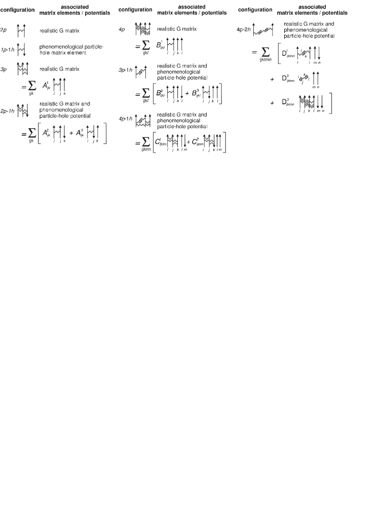
Figure 1: Factorisation of the matrix elements in terms of cluster coefficients.

are given symbolically in Fig. 1.

3 HFS in hydrogen- and lithium-like ions

With the reduction of the CMWFs and the factorization of the n-body matrix elements at our disposal we have performed calculations for the hyperfine splitting (HFS) of heavy ions [10]. In table 6 the DCM results are compared to ground-state HFS splittings calculated for a point nucleus and with results which take the finite spatial distribution of the nuclear charge into account (Breit-Schawlow correction). Additionally, QED radiative corrections [15] are listed and combined with the DCM results. The pure DCM splittings agree remarkably well with the experimental values, which are given in the last row of the table, while the wavelengths obtained after adding the QED contributions show a systematic shift to larger wavelengths. To clarify this still open point and in order to obtain further informations about the hyperfine interaction of the nucleus with the electronic cloud of high-$Z$ ions , we have also performed calculations for the HFS of the lithium-like ions. The result of the calculation [16] of the HFS for ²⁰⁹Bi⁸⁰ is given and compared with other theories in table 7. In table 7 the experimental result of Ref. [19] is also given. A new experiment will be performed at GSI (2003) in order to localize the resonance within an even smaller error. The boiling of the QED vacuum terms given in table 7, i.e. the electron-positrons contributions up to now not considered by other theories, may of course also generate a double counting effect with the QED contributions in lithium-like ions [16]. In the DCM the mixed-mode (b) states generate contributions to the HFS that may be responsible for a double counting effect with the QED perturbative calculation. The terms (b) are not considered by any perturbative calculation performed for the magnetic structure of nuclei.

4 Elastic proton scattering on exotic nuclei

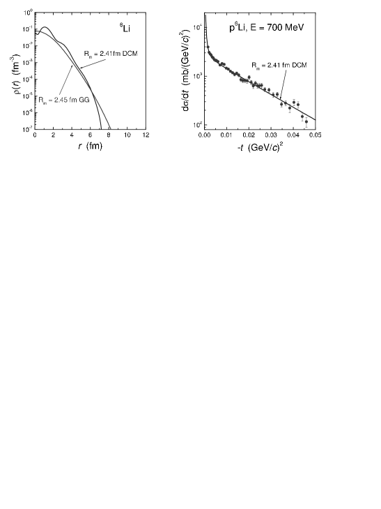
Figure 3: Left: Experimental and calculated distributions of ⁶Li; Right: experimental and theoretical proton scattering cross sections.

The transformation coefficients find also their applications in the calculation of the matter distribution of halo nuclei [20]. Here the calculation are performed for ⁶Li and ¹¹Li considering a large dimensional space and treating consistently the interaction of the valence particles with the core excitation. For ¹¹Li, in order to reproduce the three-body force we have performed calculations with three dressed neutrons [21], which are solutions of the symbolic eigenvalue equation given in Fig. 2. The results of the calculations are given in Fig. 3 and Fig. 4. In Fig. 3, we plot: (left) the experimental matter distribution calculated in Ref. [3] with the BDCM and the experimental matter distribution; and (right) the p-⁶Li experimental scattering cross sections [22] compared with the results obtained in Ref. [3] for the theoretical cross section. In Fig. 4, we plot: (left) the calculated [3] and the experimental matter distributions; (right) the calculated p-¹¹Li scattering cross sections [21] compared with the experimental one [22]. For ⁶Li the calculated and the experimental matter radii given in Fig. 3 are in good agreement with the experimental matter radius given in the figure. The calculated matter radius of ¹¹Li is 3.64 fm [21] also in good agreement with the experimental value of 3.62(19) fm [22]. The BDCM and the DCM results obtained for the scattering cross sections are in good agreement with the data of Ref. [22]. For ¹¹Li the agreement is better for momentum transfer smaller than .04 (GeV/c)², as for momentum transfer between 0.04-0.05 (GeV/c)². This is probably due to high-lying core states, which are not included in the present DCM calculations, but are of increasing importance at higher momentum transfer. The consideration of these core states will increase drastically the dimension of the CMWFs; in the calculations presented here already about two hundred components were used. However, such calculations presently under investigation become easily feasiable with the use of cluster transformation coefficients.

5 Proton polarization

The scattering cross section of low-energy photons by a structureless charged system is given by the Thomson formula which derives the photon scattering cross section only in terms of linear contributions which are proportional to the frequency of the incoming photon. A second class of terms which are linear in the frequency of the incident photon and take care of the magnetic moment and spin of the target have also been included as corrective factor to the Thomson scattering. Additionally to these linear effects, however, the cross section get contributions from terms proportional to the square of the photon frequency. These terms, are the polarization terms of Ref. [23] and modify the cross section accordingly to the square bracket of the following equation:

$${\frac{\delta\sigma}{\delta\Omega}=(\frac{\delta\sigma}{\delta\Omega})_{point}+\left[-r\left(\frac{E_{sc}}{E_{i}}\right)^{2}\frac{E_{sc}E_{i}}{(\hbar c)^{2}}\left(\frac{\alpha+\beta}{2}(1+\cos\theta)^{2}+\frac{\alpha-\beta}{2}(1-\cos\theta)^{2}\right)\right]}$$ (26)

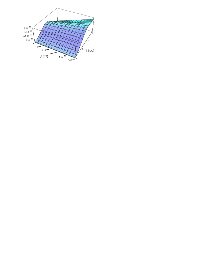
Figure 5: Scattering cross sections of high energy photons as functions of scattering angle and proton polarization parameter.

In Eq. (26), the first term $(\frac{\delta\sigma}{\delta\Omega})_{point}$ give the scattering of photons from a point-like hadron corrected with the size-spin contributions, r is the classical radius of the proton, $E_{i}$ is the incidental photon energy, $E_{sc}$ the photon scattering energy, $\theta$ the scattering angle, $\alpha$ the electric- and $\beta$ the magnetic-polarizability ı.e.: terms quadratic in the photon frequency. In Fig. 5, we plot the polarization cross section using for $\alpha$ and $\beta$ the values calculated with the model independent dispersion sum rule in Ref. [24]:

$${(\alpha+\beta)=(14.2\pm 0.03)\times 10^{-49}m^{3}}$$ (27)

These values are around those measured for the proton electric- and magnetic-polarization in Ref. [25]. The plotted polarization terms are ca. twelve order of magnitude smaller then the Compton term. Under this consideration with the present parameters of the PHELIX-laser in mind it is difficult to perform measurements to obtain the proton polarizability within a better resolution. However, additionally to the polarization effect produced by the energy of the incoming photon field, an intrinsic polarization effect [26] may contribute to the scattering cross section. This would result from effects analogous to the boiling of the QED terms. The three quarks are exciting from the vacuum in a nonlinear mechanism the $\langle q\overline{q}\rangle$ condensate. The three dressed quarks are also eigenvalues of the equation symbolically represented in Fig. 2. Calculations are in progress using for the quark the harmonic oscillator base proposed in Ref. [27]. The QCD boiling terms should then give rise to a radial distribution with an halo shape as calculated in Fig. 4 for ¹¹Li. De facto the intrinsic polarization effect increases the polarizability of the proton and may produce a sizable effect for the present parameters of PHELIX-laser. Therefore, considering this new source of polarization, experiments can reveal unexpected results.

6 Conclusion

The linearization approximation and the cluster transformation coefficients are important tools in solving nonlinear systems such as those characterizing n dressed particles: the linearization ansatz defines a collective hamiltonian that is selfconsistently solvable for the model eigenvalues, while the transformation coefficients provide easy computation for the complex n-body matrix elements which are the input to the collective eigenvalue equation. Within the linearization ansatz and the transformation coefficients, new theoretical insight have been obtained for the physics of interacting particles which coexist with the excitations of the model vacuum.

Table 1: Coefficients for the reduction $3p\Rightarrow(pp)_{J_{r}}\otimes(p)_{J_{s}}$

$V_{3,3}((3)J_{1}(3),T_{1}(1);(5,5)J_{2}(1),T_{2}(0)|\}$	$(5,5)J_{r}=1,T_{r}=1;(3)J_{s}=3,T_{s}=1)$	-0.1362
	$(5,5)J_{r}=3,T_{r}=1;(3)J_{s}=3,T_{s}=1)$	-0.0422
	$(5,3)J_{r}=1,T_{r}=1;(5)J_{s}=5,T_{s}=1)$	0.8613
	$(5,3)J_{r}=2,T_{r}=1;(5)J_{s}=5,T_{s}=1)$	-0.4876

Table 2: Coefficients for the reduction $3p1h\Rightarrow(ph)_{J_{r}}\otimes(pp)_{J_{s}}$

$T_{1,0}((3,5)J_{1}(2),T_{1}(0);(1,1)J_{2}(1),T_{2}(0)|\}$	$(3,1)J_{r}=1,T_{r}=0;(5,3)J_{s}=1,T_{s}=0)$	0.9326
	$(3,1)J_{r}=2,T_{r}=0;(5,3)J_{s}=2,T_{s}=0)$	0.3606

Table 3: Coefficients for the reduction $3p1h\Rightarrow(pp)_{J_{r}}\otimes(ph)_{J_{s}}$

$V_{1,0}((3,5)J_{1}(2),T_{1}(0);(1,1)J_{2}(1),T_{2}(0)|\}$	$(3,5)J_{r}=1,T_{r}=1;(3,1)J_{s}=2,T_{s}=0)$	0.1397
	$(3,5)J_{r}=3,T_{r}=1;(3,1)J_{s}=2,T_{s}=1)$	0.9902

Table 4: Coefficients for the reduction $4p1h\Rightarrow(3p)_{J_{r}}\otimes(ph)_{J_{s}}$

$V_{3,3}((1);(1,1)J_{1}(1),T_{1}(0);(5,1)J_{2}(2),T_{2}(1);J_{3}(1),T_{3}(1)|\}$
$(1,1,1)J_{r}=1,T_{r}=1;(5,1)J_{s}=1,T_{s}=1)$	0.9513
$(1,1,5)J_{r}=3,T_{r}=2;(1,1)J_{s}=1,T_{s}=1)$	0.3081

Table 5: Coefficients for the reduction $4p1h\Rightarrow(2p1h)_{J_{r}}\otimes(pp)_{J_{s}}$

$W_{3,3}((1)(3,5)J_{1}(1),T_{1}(0);(5,1)J_{2}(2),T_{2}(1);J_{3}(1),T_{3}(1)|\}$
$(1,1,1)J_{r}=1,T_{r}=1;(1,5)J_{s}=1,T_{s}=1)$	1.0

Table 6: Ground state hyperfine structure splittings for a point-nucleus ($E_{{\rm PN}}$), including Breit-Schawlow ($E_{{\rm BS}}$), DCM, and QED corrections. The QED contributions include vacuum polarization and self energy. All values are in eV.

	185Re74+	187Re74+	203Tl80+	205Tl80+	207Pb81+	209Bi82+
$E_{\rm PN}$	3.0103	3.0411	3.0184	2.9890	1.3998	5.8395
$E_{\rm BS}$	2.7976	2.8263	3.3073	3.3374	1.2528	5.1922
$E_{\rm tot}^{{DCM}}$	2.7192	2.7449	3.2130	3.2770	1.2166	5.0832
$\Delta E_{\rm QED}$	-0.0142	-0.0143	-0.0176	-0.0177	-0.0067	-0.0280
$E_{\rm tot}$	2.7050	2.7306	3.1954	3.2213	1.2099	5.0552
$E_{\rm exp}$	2.7187 (18)	2.7449 (18)	3.21351(25)	3.24409(29)	1.2159 (2)	5.0841 (4)
Ref.	.[11]	. [11]	[12]	[12]	.[13]	.[14]

Table 7: Comparison of different hfs calculations in meV for Li-like bismuth with experimental HFS splitting

Contribution (meV)	[17]	[18]	[16]
one-electron	958.50 (5)	958.49	958.51
charge distr.	-113.8 (3)	-151.44	-113.61
mag. distr.	-13.9 (2)	-18.68	-14.1
total QED	-4.44	-4.06	-4.81
e-e interaction	-29.45 (4)	8.43	-3.4
boiling of QED vacuum		0.06	-7.69
total theory	796.9 (2)	792.8	783.9 (3.0)
measurement [29]		820 (26) meV

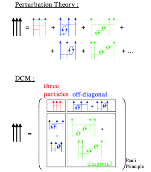
Figure 2: Simbolic representation of dressed three particles.

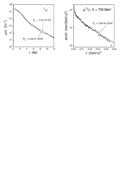
Figure 4: Left: Experimental and calculated distributions of ¹¹Li; Right: experimental and theoretical proton scattering cross sections.

References

References

- [1] [[1] ] A.L. Fetter and J.D. Walecka, Quantum Theory of Many-Particle Systems, McGraw-Hill, New York (1971).
- [2] [[2] ] M. Tomaselli, Phys. Rev. C37, 349 (1988); M. Tomaselli, Ann. Phys. (N.Y.) 205, 362 (1991).
- [3] [[3] ] M. Tomaselli, L.C. Liu, T. Kühl et al., submittet to PRC (2002).
- [4] [[4] ] M. Tomaselli, Phys. Rev. C48, 2290 (1993).
- [5] [[5] ] T. Erikson, K.F. Quader, G.E. Brown, and H.T. Fortune, Nucl. Phys. A465, 123 (1987).
- [6] [[6] ] G.E. Brown, Unified Theory of Nuclear Models, North-Holland, Amsterdam 1964; A.M. Lane, Nuclear Theory, W.A. Benjamin Inc., New York (1964).
- [7] [[7] ] D.J. Rowe, Nuclear Collective Motion, Methmen and Co. Ltd., London (1970).
- [8] [[8] ] E.P. Wigner, Group theory, Academic Press, New York (1959).
- [9] [[9] ] G. Racah, CERN Report No. 61.8 (1961); A. de-Shalit and I. Talmi,Nuclear Shell Theory, Academic Press, New York (1963).
- [10] [[10] ] M. Tomaselli, S.M. Schneider, E. Kankeleit, and T. Kühl, Phys. Rev. C51, 2989 (1995); M. Tomaselli, T. Kühl, P. Seelig, C. Holbrow, and E. Kankeleit, Phys. Rev. C58, 1524 (1998); M. Tomaselli, T. Kühl, W. Nörtershäuser, S. Borneis, A. Dax, D. Marx, H. Wang, and S. Fritzsche, Phys. Rev. A65, 022502 (2002).
- [11] [[11] ] J. R. Crespo López-Urrutia, P. Beiersdorfer, K. Widmann, B. B. Birkett, A.-M. Mårtensson-Pendrill and M. G. H. Gustavsson, Phys. Rev. A 57, 879 (1998).
- [12] [[12] ] P. Beiersdorfer et al., Phys. Rev. A 64, 032506 (2001).
- [13] [[13] ] I. Klaft et al., Phys. Rev. Lett. 73, 2425 (1993).
- [14] [[14] ] P. Seelig et al., Phys. Rev. Lett. 81, 4824 (1998).
- [15] [[15] ] V.M. Shabaev, M. Tomaselli, T. Kühl, A.N. Artemyev, and V.A. Yerokhin, Phys. Rev. A 56, 252 (1997); S. M. Schneider, W. Greiner, G. Soff, Phys. Rev. A 50, 118 (1994); H. Person, S. M. Schneider, G. Soff, W. Greiner, Phys. Rev. Lett. 76, 1433 (1996); P. Sunergren, H. Persson, S. Salomonson, S. M. Schneider, I. Lindgren, and G. Soff, Phys. Rev. A 58, 1055 (1998).
- [16] [16] M. Tomaselli, T. Kühl, W. Nörtershäuser, G. Ewald, R. Sanchez, S. Fritzsche, and S.G. Karshenboim, Can. J. Phys., 2002 to be published.
- [17] [[17] ] V. M. Shabaev et al., Phys. Rev. A 57, 149 (1998).
- [18] [[18] ] S. Bouchard and P. Indelicato, Eur. Phys. J. D 8, 59 (2000).
- [19] [[19] ] P. Beiersdorfer et al., Phys. Rev. Lett. 80, 3082 (1998).
- [20] [[20] ] I. Tanihata et al., Nucl. Phys. A488, 113 (1988).
- [21] [[21] ] M. Tomaselli, T. Kühl, P. Egelhof, W. Nörtershäuser, C. Kozhuharov, A. Dax, H. Wang, S.R. Neumaier, D. Marx, H.-J. Kluge I. Tanihata, S. Fritzsche, and M. Mutterer, Proc. Conf. Nuclear Physics at Border Lines (NPBL), Lipari (Messina), Italy, 2001, Edited G. Fazio, G. Giardina, F. Hanappe, G. Imme’ and N. Rowley, World Scientific, ISBN 981-02-4778-8, 336 (2002); M. Tomaselli et al., Proc. Conf. Dynamical Aspects of Nuclear Fission (DANF), ast-Papiernicka (2001), in press.
- [22] [[22] ] A.V. Dobrowolsky et al., Proc. Conf. Nuclear Physics at Border Lines (NPB), Lipari (Messina), Italy, 2001, Edited G. Fazio, G. Giardina, F. Hanappe, G. Imme’ and N. Rowley, World Scientific, ISBN 981-02-4778-8, 336 (2002).
- [23] [[23] ] V.A. Petrun’kin, Soviet Physics JETP 13, 808 (1961).
- [24] [[24] ] F.J. Federspiel et al., Phys. Rev. Lett. 67, 1511 (1991).
- [25] [[25] ] V. Olmos de Leon et al., Eur. Phys. J. A10, 207 (2001).
- [26] [[26] ] M. Tomaselli, L. C. Liu, T. Kühl, D. Ursescu, in preparation.
- [27] [[27] ] P. Geiger and N. Isgur, Phys. Rev. D55, 299 (1997).
- [28]