Vacuum polarization by a magnetic flux of special rectangular form

Abstract

We consider the ground state energy of a spinor field in the background of a square well shaped magnetic flux tube. We use the zeta- function regularization and express the ground state energy as an integral involving the Jost function of a two dimensional scattering problem. We perform the renormalization by subtracting the contributions from first several heat kernel coefficients. The ground state energy is presented as a convergent expression suited for numerical evaluation. We discuss corresponding numerical calculations. Using the uniform asymptotic expansion of the special functions entering the Jost function we are able to calculate higher order heat kernel coefficients.

1 Introduction

Since the classical work [1] of H.B.G. Casimir, where the energy of vacuum polarized by two conducting planes was calculated, a number of similar problems was investigated for various external conditions (boundary conditions, background potentials etc.), see, for example, the recent review [2] or the books [3, 4] . No general rule for the dependence of the vacuum energy on the background properties has been found so far. In particular, it is unknown how to forecast the sign of the energy.

An interesting problem is the calculation of the vacuum energy of a spinor field in the background of a magnetic field. This problem was first considered as early as in 1936 by W. Heisenberg and H. Euler [5] who were interested in the effective action in the background of a homogeneous magnetic field.

Presently, the interest is shifted to string like configurations. In [6] the contribution of the fermionic ground state energy to the stability of electro weak strings was addressed. In [7] the gluonic ground state energy in the background of a center-of-group vortex in QCD had been considered.

A very special inhomogeneous reflectionless magnetic background is for example the model for domain wall [8]. In this case, the equation for the vacuum fluctuations was easy to solve analytically. However, the final expression for the effective action involves an additional integration over a momentum, thus bringing no real simplifications.

In QED, for the background of a flux tube with constant magnetic field inside the ground state energy was calculated in [13]. Here it turned out to be negative remaining of course much smaller than the classical energy of the background field.

An interesting approach is that used in [10] where the issue of the sign and of bounds on fermionic determinants in a magnetic background had been considered.

The remarkably simple case of a magnetic background field concentrated on a cylindrical shell (i.e., a delta function shaped profile) was considered in [11]. Here different signs of the vacuum energy turned out to be possible in dependence on the parameters (radius and flux).

In general, the issue of stability of the strings is of interest. In electro weak theory, and in QED in particular, the coupling is small. Hence the vacuum energy as being a one loop correction to the classical energy is suppressed by this coupling. While in QED a magnetic string is intrinsically unstable, in electro weak theory there are unstable and stable configuration known [12]. Here quantum corrections may become important for the stability. A question of special interest is whether a strong or singular background may have a quantum vacuum energy comparable to the classical one.

For the calculation of ground state energy, it is necessary to subtract the ultraviolet divergences. This procedure is in general well known and we follow . Roughly speaking one has to subtract the contribution of the first few heat kernel coefficients ($a_{0}$ through $a_{2}$ in the given case of (3+1) dimensions). After that one can remove the intermediate regularization and one is left with finite expressions. However, in order to obtain these finite expressions in a form suitable for numerical calculations one has to go one more step. As described in , see also below in section 2, one has to add and to subtract of a certain part of the asymptotic expansion of the integrand.

In the present paper we generalize the analysis done in [9] to a rectangular shaped magnetic background field. So we consider the vacuum energy of a spinor field in QED for a background as given by Eqs. (2.1, 2.5). This problem is technically more involved and allows progress in two directions. First, it allows to refine the mathematical and numerical tools for such problems and, second, it allows to address the question how the vacuum energy behaves for an increasingly singular background (making the rectangle narrower). So this model interpolates to some extend between the flux tube with homogeneous field inside in [9] and the delta shaped one in [11].

The basic principles of this procedure are described briefly in Sec. 2. Namely it starts with the well known zeta functional regularization. The regularized ground state energy is represented as a zeta function of a hamiltonian spectrum and treated in termini of heat kernel expansion. The representation of regularized ground state energy as an integral of the logarithmic derivative of the Jost function for spinor wave scattering problem on the external magnetic background is obtained. The Jost function is obtained from the exact solutions of Dirac equation, derived in Sec. 3. The explicit form of the exact and asymptotic Jost function is considered in Sec. 4. In Sec.5 the representation useful for further numerical evaluations is derived. Sec. 6 is devoted to the calculation of the heat kernel coefficient $a_{5/2}$ and the Sec. 7 contains some numerical evaluations of the ground state energy. The divergent part is identified as that part of the corresponding heat kernel expansion which does not vanish for large $m$ (mass of the quantum spinor field). After the subtraction of this divergent part the remaining analytical expression must be transformed in order to lift the regularization. A part of the uniform asymptotic expansion of the Jost function is used for this procedure. Finally the analytical expression for the ground state energy has been evaluated numerically.

Throughout the paper $\hbar=c=1$ is used.

2 The renormalized ground state energy

Consider a spinor field on a magnetic background $\vec{B}$ of the form

$$\vec{B}=\frac{\Phi}{2\pi}{h(r)}\vec{e_{z}}$$ (2.1)

where $\Phi$ is constant defining the magnetic flux, $\vec{e_{z}}$ is a unit vector in the cylindrical coordinate system ($r,\phi,z$). The Lagrangian is

$${\cal L}=-\frac{1}{4}F_{\mu\nu}F^{\mu\nu}+\bar{\psi}\left[i\gamma^{\mu}(\partial_{\mu}+eA_{\mu})-m\right]\psi.$$ (2.2)

The potential $\vec{A}(r)$

$$\vec{A}=\frac{\Phi}{2\pi}\frac{a(r)}{r}\vec{e_{\varphi}}$$ (2.3)

possesses cylindrical symmetry and the radial part $a(r)$ is taken to be

$$a(r)=\left\{\begin{array}[]{c}0,\hfill r<R_{1},R_{2}\\ \frac{1}{\kappa}(\frac{r^{2}}{R_{1}^{2}}-1)\ R_{1}\leq r\leq R_{2}\\ 1,r>R_{1},R_{2}\end{array}\right.\\$$ (2.4)

The profile function for the magnetic field is

$$\ \ h(r)=\frac{1}{r}\frac{\partial}{\partial r}a(r)=\left\{\begin{array}[]{c}0,\hfill r<R_{1},R_{2}\\ \frac{2}{\kappa R^{2}_{1}}R_{1}\leq r\leq R_{2}\\ 0,r>R_{1},R_{2}\end{array}\right.$$ (2.5)

with $\kappa=\frac{R_{2}^{2}-R_{1}^{2}}{R_{1}^{2}}$.The shape of the background can be interpreted geometrically as an infinitely long flux tube empty inside.

We use the zeta-function regularization for the vacuum energy $E_{0}$. Since the background is static, the following representation holds,

$$E_{0}(s)=-\frac{1}{2}\mu^{2s}\sum\limits_{(n)}\omega_{(n)}^{1-2s},$$ (2.6)

where

$$\omega_{(n)}=\epsilon_{(n)}=\sqrt{\vec{p}^{2}+m^{2}}$$

are eigenfrequences resp. eigenvalues of energy for one particle states, (the spectrum of the corresponding hamiltonian, see the next section), $\mu$ is a parameter with the dimension of mass which is introduced to keep the correct dimension of energy in this expression.

For technical reasons we assume that the system is contained in a large but finite cylinder of radius $R$ in order to have discrete eigenvalues in the transversal directions. Because of the translational invariance along the z-axis we can separate the $z$-component of momentum,

$$E_{0}(s)=-\frac{1}{2}\mu^{2s}\int\limits_{-\infty}^{\infty}\frac{dp_{z}}{2\pi}\sum\limits_{(n)}(p_{z}^{2}+k_{(n)}^{2}+m^{2})^{\frac{1}{2}-s}.$$ (2.7)

Here is it necessary to remark that $E_{0}$ has the meaning of density per unit length. Integrating out $p_{z}$ we get

$$E_{0}(s)=-\mu^{2s}\frac{1}{4\sqrt{\pi}}4\frac{\Gamma(s-1)}{\Gamma(s-\frac{1}{2})}\sum\limits_{(n)}(k_{(}n)^{2}+m^{2})^{1-s}.$$ (2.8)

In this expression a factor 4 resulting from the summation over spin states and over the sign of the one particle energies appeared. The remaining sum over $(n)$ is over the eigenvalues $k_{(}n)$ of a two dimensional wave equation for one mode in the perpendicular plane. The further transformation of this expression is described more detailed in [9], [16], [15]. The first step is based on the property of logarithmic derivative of eigenfunctions with respect to momentum k. The contour integral,

$$\int\limits_{\gamma}\frac{dk}{2\pi i}(k^{2}+m^{2})^{1-s}\partial_{k}\ln\phi_{l}(kr),$$

is equal to the sum over the spectrum, $\sum\limits_{(n)}(k_{n}^{2}+m^{2})^{1-s}$, if the contour $\gamma$ encircles the real positive axis. Then (2.8) becomes

$$E_{0}(s)=-\mu^{2s}\frac{1}{\sqrt{\pi}}\frac{\Gamma(s-1)}{\Gamma(s-\frac{1}{2})}\sum\limits_{l=-\infty}^{\infty}\int\limits_{\gamma}\frac{dk}{2\pi i}(k^{2}+m^{2})^{1-s}\partial_{k}\ln\phi_{l}(kr).\\$$ (2.9)

Here $\phi_{l}(r)$ are the eigenfunctions of hamiltonian $\hat{H}$ labeled by the orbital momentum $l$.

In the present formalism instead of wave functions $\phi_{l}(r)$ we use the corresponding Jost functions $f_{l}(k)$ which contain all necessary informations on the spectrum of scattering problem. For the space domain outside of cylindrical magnetic background, at $r>R_{2}$, the wave functions can be chosen as a linear composition of Hankel functions

$$\phi_{l}(kr)=\frac{1}{2}[\bar{f_{l}}(k)H^{(1)}_{l}(kr)+f_{l}(k)H^{(2)}_{l}(kr)],\\$$ (2.10)

where $\bar{f}_{l}(k)$ and $f_{l}(k)$ are the corresponding Jost functions.

Now after the subtraction of contribution from empty Minkowski space (identified as the term divergent at $R\rightarrow\infty$, which is independent of the background and corresponds to the heat kernel coefficient $a_{0}$,(2.15) below), and rotation of the path towards the imaginary positive axis one obtains [9]

$$E_{0}(s)=\\ -\frac{1}{\sqrt{\pi}}\frac{\Gamma(s-1)}{\Gamma(s-\frac{1}{2})}\frac{\sin\pi s}{\pi}\sum\limits_{l=-\infty}^{\infty}\int\limits_{m}^{\infty}dk(k^{2}-m^{2})^{1-s}\partial_{k}\ln f_{l}(ik),$$ (2.11)

which is a very useful representation of the regularized ground state energy. A merit of this representation is the absence of oscillations of the integrand for large arguments.

To discuss divergences in $E_{0}$ we need a more general setting. $E_{0}(s)$ can be expressed through the zeta-function of the associated differential operator $\bf{\hat{P}}$

$$E_{0}(s)=-\frac{\mu^{2s}}{2}\zeta_{(\bf{\hat{P}})}(s-\frac{1}{2}).$$ (2.12)

$\zeta_{(\bf{\hat{P}})}(s)$ admits an integral representation

$$\zeta_{\bf{\hat{P}}}(s)=\int\limits_{0}^{\infty}dt\frac{t^{s-1}}{\Gamma(s)}K(t)$$ (2.13)

where the kernel of this integral representation $K(t)=\sum\limits_{n}e^{-t(k_{(n)}^{2}+m^{2})}$ is the so called heat kernel. The associated “heat kernel expansion” for the kernel $K(t)$ of this integral representation at $t\rightarrow 0$ is [17]

$$K(t)\sim\frac{e^{-tm^{2}}}{(4\pi t)^{3/2}}\sum\limits_{n\geq 0}a_{n}t^{n}\ .$$ (2.14)

In accordance to the heat kernel expansion, the coefficients $a_{n}$ occurred in (2.14) must be for our background [17]:

$$a_{0}=V$$ (2.15)

is simple an (infinite) volume of configuration space; the part proportional to it has been even dropped before during the renormalization procedure as a contribution of the empty Minkowski space. All other coefficients up to $a_{2}$ for this background must be zero through dimensional reasons and requirement of gauge invariance, (for details see the paper [18]).

$$a_{1/2}=a_{1}=a_{3/2}=0.$$ (2.16)

The first nonzero coefficient is known to read

$$a_{2}=\frac{2}{3}F^{2}_{\mu\nu}$$ (2.17)

and only the term with $n=2$ contributes to the “divergent” part of energy [11], [9]. It will be shown below that only the contribution proportional to $a_{2}$ in $E_{0}(s)$ contains a simple pole at $s\rightarrow 0$ and in the case of pure magnetic background is proportional to the classical energy

$$E^{class}=\frac{1}{2}\vec{B}^{2}=\frac{8e^{2}}{3}a_{2}\$$ (2.18)

In the paper [9] it has been found, that the regularized ground state energy of the magnetic flux tube of finite radius $R$ behaves as $~{}\frac{R^{-3}}{m}$ at $R\rightarrow\infty$ which corresponds to the contribution proportional to $a_{5/2}$. It holds in accordance to the observed fact that in the case of non-smooth backgrounds the heat kernel coefficients with half-integer number starting from some value corresponding to the smoothness-class of the background are different from zero. It occurs namely in our case, where the background potential $\vec{A}(r)$ is continous and the magnetic field $h(r)$ has a discontinuity. The coefficient $a_{5/2}$ is nonzero in our case, see below Sec.6. The next terms of this asymptotic may be $~{}\frac{R^{-4}}{m^{2}}$ corresponding to $a_{3}$, and $a_{4}$ delivering terms $~{}\frac{R^{-6}}{m^{4}}$.

We define the renormalized ground state energy as

$$E^{ren}=E_{0}-E^{div},$$ (2.19)

where $E^{div}$ is obtained from the heat kernel expansion (2.14) and $E^{ren}$ fulfills the normalization condition [19]

$$\lim E^{ren}=0\ \ at\ \ m\rightarrow\infty.$$ (2.20)

Inserting the heat kernel expansion (2.14) into the zeta function and using (2.12) we have

$$E^{div}=\frac{a_{2}}{32\pi^{2}}(\frac{1}{s}-2+ln\frac{4\mu^{2}}{m^{2}}),$$ (2.21)

where $a_{2}$ is the only non-zero heat kernel coefficient $a_{n},\ 0<n\leq 2$, contributing to the divergent part of vacuum energy.

For the renormalized ground state energy the asymptotical dependence on powers of $m$ at $m\rightarrow\infty$ follows from Eq.(2.14) to have the form

$$E_{0}^{ren}\stackrel{{\scriptstyle\sim}}{{{}_{m\rightarrow\infty}}}\sum\limits_{n>2}\frac{e_{n}}{m^{2n}}$$ (2.22)

with some coefficients $e_{n}$.

In accordance with the interpretation of $E^{ren}$ it must vanish in the limit of $m\rightarrow\infty$ since it is the energy of vacuum fluctuations. Through the subtraction of terms containing all non-negative powers of $m^{2}$ (which are the terms of heat kernel expansion up to $a_{2}$) the condition (2.20) is satisfied automatically.

Some comments on the subtraction scheme are in order. This scheme is motivated by the physical assumption that the quantum fluctuations should vanish if the mass of the fluctuating field becomes large. The scheme had been used in a number of Casimir energy calculations. In [20] it had been shown to be equivalent to the so called “no tadpole” normalization condition which is common in field theory. It should be noticed that this scheme does not apply to massless fluctuating fields, for a discussion of this point see [21].

So $E^{ren}$ as given by Eq.(2.19)is now finite at $s\rightarrow 0,$ but it is not possible to use this expression immediately since the integral in this limit does not exist; i.e. one cannot carry out the analytical continuation to $s=0$. In order to get a representation where this can be done one can make a trick [22], namely add and subtract a part $\ln f_{l}^{asym}$ of the uniform asymptotical expansion for $\ln f_{l}$ in (2.11) containing a minimal number of terms to provide the convergence of the remaining part after the subtraction. Thus we can separate the resulting expression into four terms

$$E^{ren}=(E_{0}-E^{asym})+(E^{as}-E^{div})$$ (2.23)

where

$$E^{asym}=2C_{s}\sum\limits_{l}\int\limits_{m}^{\infty}dk(k^{2}-m^{2})^{1-s}\frac{\partial}{\partial k}\ln f_{l}^{asym}(ik)$$ (2.24)

and redefine two terms in brackets as

$$E^{ren}=E^{f}+E^{as}$$

$$E^{f}=E_{0}-E^{asym}$$ (2.25)

$$E^{as}=E^{asym}-E^{div},$$ (2.26)

thus $E^{f}$ is defined to be

$$E^{f}=\frac{1}{2\pi}\sum\limits_{l=-\infty}^{\infty}\int\limits_{m}^{\infty}dk\ (k^{2}-m^{2})\frac{\partial}{\partial k}[lnf_{l}(ik)-\ln f^{as}_{l}(ik)]$$ (2.27)

The “finite” part $E^{f}$ of the renormalized vacuum energy is not only well defined at $s\rightarrow 0$, but also provides a representation well suited for numerical analysis. The analytical continuation for $E^{as}$ at this limit will be constructed below.

3 Solution of the Dirac equation

We consider a spinor quantum field $\psi$ in the background of the classical magnetic flux. We start with the Dirac equation for this field

$$\left\{i\gamma^{\mu}\frac{\partial}{\partial x^{\mu}}-m-e\gamma^{\mu}A_{\mu}\right\}\psi=0$$ (3.1)

with the electromagnetic potential (2.3). The $\psi$ in (3.1) is a spinor quantum field of mass $m$ and charge $e$, interacting with $\vec{A}$ (2.3). The gamma matrices in our representation are chosen to be the same as in [23]

$$\gamma^{0}=\left\{\begin{array}[]{cc}\sigma_{3}&0\\ 0&-\sigma_{3}\end{array}\right\}\ \ \ \ \ \gamma^{1}=\left\{\begin{array}[]{cc}i\sigma_{2}&0\\ 0&-i\sigma_{2}\end{array}\right\}\\ \\ \gamma^{2}=\left\{\begin{array}[]{cc}-i\sigma_{1}&0\\ 0&i\sigma_{1}\end{array}\right\}\ \ \ \ \ \gamma^{3}=\left\{\begin{array}[]{cc}0&1\\ -1&0\end{array}\right\}.$$ (3.2)

Now we follow the standard procedure and separate the variables. Using the ansatz

$$\phi(r,\varphi,z)=e^{-ip_{0}x^{0}}e^{-ip_{z}z}\Psi(r,\varphi)\\$$ (3.3)

we obtain the equation for the 4- component spinor $\Psi=\left[\begin{array}[]{c}\phi\\ \chi\end{array}\right]$

$$\left\{\begin{array}[]{cc}p_{0}+\hat{L}-m\sigma_{3}&p_{3}\sigma_{3}\\ \\ p_{3}\sigma_{3}&p_{0}+\hat{L}+m\sigma_{3}\end{array}\right\}\Psi=0,$$ (3.4)

where $\hat{L}=i\sum\limits_{i=1}^{2}\sigma_{i}(\partial_{i}+ieA_{i})$, $\phi,\chi$ are the two-component spinors.

Respecting the translational invariance of the system it is sufficient to solve the equations only for $p_{3}=0$. Then one of the two decoupled equations $(\phi,\chi)$ reads

$$\left\{\begin{array}[]{cc}p_{0}-m&\frac{\partial}{\partial r}-\frac{l-\delta a(r)}{r}\\ \\ -\frac{\partial}{\partial r}-\frac{l+1-\delta a(r)}{r}&p_{0}+m\end{array}\right\}\Phi(r)=0$$ (3.5)

(here the standard ansatz

$$\Phi=\left[\begin{array}[]{c}i\psi^{u}(r)e^{-i(l+1)\varphi}\\ \\ \psi^{l}(r)e^{-il\varphi}\end{array}\right]$$ (3.6)

has been used, $l$ is the orbital quantum number), the radial part denoted as

$$\Phi(r)=\left\{\begin{array}[]{c}\psi^{u}(r)\\ \\ \psi^{l}(r)\end{array}\right\}$$ (3.7)

and

$$\delta=\frac{e\Phi}{2\pi}.$$ (3.8)

In order to use later the symmetry properties of the Jost function we redefine the parameter $l$ in (3.6) (orbital number) as $\nu$ according to

$$\nu=\left\{\begin{array}[]{c}l+\frac{1}{2}\ for\ l=0,1,2,...\\ \\ -l-\frac{1}{2}\ for\ l=-1,-2,...\end{array}\right.$$ (3.9)

For the given construction of potential (2.4) we get three equations and three types of solutions for 3 areas of space respectively
Domain I: $r<R_{1}$. The free wave equation (the magnetic flux is zero), the solutions are the Bessel functions $J_{\nu\pm\frac{1}{2}}(kr)$

$$\Phi_{I}^{-}(r)=\left[\begin{array}[]{c}\psi^{u-}_{I}(r)\\ \\ \psi^{l-}_{I}(r)\end{array}\right]={\frac{1}{\sqrt{p_{0}-m}}\left[\begin{array}[]{c}-\sqrt{p_{0}+m}J_{\nu-\frac{1}{2}}(kr)\\ \\ \sqrt{p_{0}-m}J_{\nu+\frac{1}{2}}(kr)\end{array}\right]},$$ (3.12)

$$\Phi_{I}^{+}(r)=\left[\begin{array}[]{c}\psi^{u+}_{I}(r)\\ \\ \psi^{l+}_{I}(r)\end{array}\right]={\frac{1}{\sqrt{p_{0}-m}}\left[\begin{array}[]{c}\sqrt{p_{0}+m}J_{\nu+\frac{1}{2}}(kr)\\ \\ \sqrt{p_{0}-m}J_{\nu-\frac{1}{2}}(kr)\end{array}\right]}$$ (3.15)

$p_{0}=\sqrt{m^{2}-k^{2}}$
This solution of equation (3.5) in the domain I is chosen to be the so called regular solution which is defined as to coincide for $r\rightarrow 0$ with the free solution.
Domain II: $R_{1}<r<R_{2}$ The equation with a homogeneous magnetic field
has the solution

$$\Phi_{II}^{-}(r)=C_{r}^{-}\left[\begin{array}[]{c}\psi^{u-}_{II.r}(r)\\ \\ \psi^{l-}_{II.r}(r)\end{array}\right]+C_{i}^{-}\left[\begin{array}[]{c}\psi^{u-}_{II.i}(r)\\ \\ \psi^{l-}_{II.i}(r)\end{array}\right]=$$ (3.18)

$$C_{r}^{-}\left[\begin{array}[]{c}\frac{(p_{0}+m)}{2(\tilde{\alpha}+1)}r^{\tilde{\alpha}+1}e^{-\frac{\beta r^{2}}{4}}{{}_{1}}F_{1}(1-\frac{k^{2}}{2\beta},\tilde{\alpha}+2;\frac{\beta r^{2}}{2})\\ \\ \hfill r^{\tilde{\alpha}}e^{-\frac{\beta r^{2}}{4}}{{}_{1}}F_{1}(-\frac{k^{2}}{2\beta},\tilde{\alpha}+1;\frac{\beta r^{2}}{2})\end{array}\right]$$ (3.20)

(3.21)

$$+C_{i}^{-}\left[\begin{array}[]{c}\frac{1}{p_{0}-m}\frac{2\tilde{\alpha}}{r}(\frac{\beta r^{2}}{2})^{-\tilde{\alpha}}e^{-\frac{\beta r^{2}}{4}}{{}_{1}}F_{1}(-\frac{k^{2}}{2\beta}-\tilde{\alpha},-\tilde{\alpha};\frac{\beta r^{2}}{2})\\ \\ (\frac{\beta r^{2}}{2})^{-\tilde{\alpha}}e^{-\frac{\beta r^{2}}{4}}{{}_{1}}F_{1}(-\frac{k^{2}}{2\beta}-\tilde{\alpha},1-\tilde{\alpha};\frac{\beta r^{2}}{2})\end{array}\right].$$ (3.23)

$\Phi_{II}^{+}(r)$ is the same, but $\tilde{\alpha}$ replaced by $\alpha$
here: $\alpha=\nu-\frac{1}{2}+\frac{\delta}{\kappa}$ for $l\geq 0$
                 $\tilde{\alpha}=\frac{\delta}{\kappa}-\nu-\frac{1}{2}$ for $l<0$
                 $\beta=\frac{2\delta}{\kappa R_{1}^{2}}$
${{}_{1}}F_{1}$ is a confluent hypergeometric function [24], [25].

The coefficients $C_{i},C_{r}$ are some constants that will be irrelevant for expressing the Jost function. The indices u and l denote “upper” and “lower” components of spinor respectively. The lower index “i” or “r” corresponds to “regular” or “irregular” part of solutions dependent on the behaviour of the function if continued to $r=0$. If the external background vanishes ($\delta\rightarrow 0$), contributions of irregular parts to the solution disappear.
Domain III: $r>R_{2}$ The free wave equation outside of the magnetic flux has the solutions

$$\Phi_{III}^{-}(r) = \frac{1}{2}\bar{f}^{-}_{\nu}(k)\frac{1}{\sqrt{p_{0}-m}}\left[\begin{array}[]{c}\psi^{u-}_{III.r}(r)\\ \\ \psi^{l-}_{III.r}(r)\end{array}\right]+\frac{1}{2}f^{-}_{\nu}(k)\frac{1}{\sqrt{p_{0}-m}}\left[\begin{array}[]{c}\psi^{u-}_{III.i}(r)\\ \\ \psi^{l-}_{III.i}(r)\end{array}\right]$$ (3.26)

$$= \frac{1}{2}\bar{f}^{-}_{\nu}(k)\left[\begin{array}[]{r}-\eta H^{(1)}_{\nu-\frac{1}{2}+\delta}(kr)\\ \\ H^{(1)}_{\nu+\frac{1}{2}+\delta}(kr)\end{array}\right]+\frac{1}{2}f^{-}_{\nu}(k)\left[\begin{array}[]{r}-\eta H^{(2)}_{\nu-\frac{1}{2}+\delta}(kr)\\ \\ H^{(2)}_{\nu+\frac{1}{2}+\delta}(kr)\end{array}\right],$$ (3.29)

$$\Phi_{III}^{+}(r) = \frac{1}{2}\bar{f}^{+}_{\nu}(k)\frac{1}{\sqrt{p_{0}-m}}\left[\begin{array}[]{c}\psi^{u+}_{III.r}(r)\\ \\ \psi^{l+}_{III.r}(r)\end{array}\right]+\frac{1}{2}f^{+}_{\nu}(k)\frac{1}{\sqrt{p_{0}-m}}\left[\begin{array}[]{c}\psi^{u+}_{III.i}(r)\\ \\ \psi^{l+}_{III.i}(r)\end{array}\right]$$ (3.32)

$$= \frac{1}{2}\bar{f}^{+}_{\nu}(k)\left[\begin{array}[]{r}\eta H^{(1)}_{\nu+\frac{1}{2}-\delta}(kr)\\ \\ H^{(1)}_{\nu-\frac{1}{2}-\delta}(kr)\end{array}\right]+\frac{1}{2}f^{+}_{\nu}(k)\left[\begin{array}[]{r}\eta H^{(2)}_{\nu+\frac{1}{2}-\delta}(kr)\\ \\ H^{(2)}_{\nu-\frac{1}{2}-\delta}(kr)\end{array}\right],$$ (3.35)

$$\eta = \frac{\sqrt{p_{0}+m}}{\sqrt{p_{0}-m}}$$

and $f_{\nu}(k)$ is the desired Jost function in accordance to the definition ( 2.10). The functions $f_{l}(-k)$ and $\bar{f}_{l}(k)$ are conjugated to each other because of the choice of the solution in the domain I to be regular (3).

4 The exact and asymptotic Jost function for the background

To obtain a Jost function we need to impose certain matching conditions for the spinor wave at the boundaries between I-II and II-III domains. It is known that for a continuous potential $a(r)$ as we consider here, the spinor wave function must be continuous, hence for its components it holds

$$\Phi_{II}^{\mp}(r)=\Phi_{I}^{\mp}(r)\Big{|}_{r=R_{1}},$$

$$\Phi_{III}^{\mp}(r)=\Phi_{II}^{\mp}(r)\Big{|}_{r=R_{2}}$$ (4.1)

Resolving these equations for $f_{\nu}^{\pm}$ we obtain, that

$$f_{\nu}^{\pm}(k) = 2\frac{A+B}{W_{III}W_{II}}$$

$$A = (\psi_{I}^{u\pm}\psi_{II.i}^{l\pm}-\psi_{I}^{l\pm}\psi_{II.i}^{u\pm})\Big{|}_{R_{1}}(\psi_{II.r}^{u\pm}\psi_{III.r}^{l\pm}-\psi_{II.r}^{l\pm}\psi_{III.r}^{u\pm})\Big{|}_{R_{2}},$$

$$B = (\psi_{I}^{l\pm}\psi_{II.r}^{u\pm}-\psi_{I}^{u\pm}\psi_{II.r}^{u\pm})\Big{|}_{R_{1}}(\psi_{II.i}^{u\pm}\psi_{III.r}^{l\pm}-\psi_{II.i}^{l\pm}\psi_{III.r}^{u\pm})\Big{|}_{R_{2}}$$ (4.2)

The denominator of this expression can be written using the Wronskians of hypergeometric and Bessel functions as follows

$$W_{III}=(\psi_{III.i}^{u}\psi_{III.r}^{l}-\psi_{III.i}^{l}\psi_{III.r}^{u})\Big{|}_{R_{2}}=(\frac{p_{0}+m}{p_{0}-m})^{\frac{1}{2}}\frac{4i}{\pi kR_{2}}$$

(4.3)

$$W_{II}=(\psi_{II.r}^{u}\psi_{II.i}^{l}-\psi_{II.r}^{l}\psi_{II.i}^{u})\Big{|}_{R_{1}}=-\frac{\alpha\beta}{p_{0}-m}(\frac{\beta R_{1}}{2})^{-\alpha-1}$$ (4.4)

To calculate $E_{0}$ we need this function with imaginary argument (2.11) so we need to replace $k$ by $ik$. As a result we obtain the new expression for $f(ik)$ that contains now modified Bessel functions $I_{\nu\pm\frac{1}{2}}$ instead of $J_{\nu\pm\frac{1}{2}}$ and modified Bessel functions $K_{\nu\pm\frac{1}{2}\mp\delta}$ instead of $H^{(1,2)}_{\nu\pm\frac{1}{2}\mp\delta}$.

$$f^{+}_{\nu}(ik) = \frac{\pi kR_{1}R_{2}e^{-\delta/\kappa+\frac{i\pi\delta}{2}}}{\frac{1}{2}-\tilde{\nu}}\times$$

$$\left\{\left[\frac{kR_{1}}{2\tilde{\nu}+1}\ {{}_{1}}F_{1}(1+\frac{k^{2}}{2\beta},\ \tilde{\nu}+\frac{3}{2};\ \frac{\beta R_{1}^{2}}{2})\ I_{\nu-\frac{1}{2}}(kR_{1})-\right.\right.$$

$$\left.\hskip 113.81102pt{{}_{1}}F_{1}(\frac{k^{2}}{2\beta},\ \tilde{\nu}+\frac{1}{2};\ \frac{\beta R_{1}^{2}}{2})\ I_{\nu+\frac{1}{2}}(kR_{1})\right]\times$$

$$\left[\frac{2\tilde{\nu}+1}{R_{2}}\ {{}_{1}}F_{1}(\frac{1}{2}-\tilde{\nu}+\frac{k^{2}}{2\beta},\ \frac{1}{2}-\tilde{\nu};\ \frac{\beta R_{2}^{2}}{2})\ K_{\nu-\frac{1}{2}-\delta}(kR_{2})-\right.$$

$$\left.\hskip 113.81102ptk\ {{}_{1}}F_{1}(\frac{1}{2}-\tilde{\nu}+\frac{k^{2}}{2\beta},\ \frac{3}{2}-\tilde{\nu};\ \frac{\beta R_{2}^{2}}{2})\ K_{\nu+\frac{1}{2}-\delta}(kR_{2})\right]-$$

$$\left[k\ {{}_{1}}F_{1}(\frac{1}{2}-\tilde{\nu}+\frac{k^{2}}{2\beta},\ \frac{3}{2}-\tilde{\nu};\ \frac{\beta R_{1}^{2}}{2})\ I_{\nu+\frac{1}{2}}(kR_{1})+\right.$$

$$\left.\hskip 113.81102pt\frac{2\tilde{\nu}-1}{R_{1}}\ {{}_{1}}F_{1}(\frac{1}{2}-\tilde{\nu}+\frac{k^{2}}{2\beta},\ \frac{1}{2}-\tilde{\nu};\ \frac{\beta R_{1}^{2}}{2})\ I_{\nu-\frac{1}{2}}(kR_{1})\right]\times$$

$$\left[\frac{kR_{2}}{2\tilde{\nu}+1}\ {{}_{1}}F_{1}(1+\frac{k^{2}}{2\beta},\ \tilde{\nu}+\frac{3}{2};\ \frac{\beta R_{2}^{2}}{2})\ K_{\nu-\frac{1}{2}-\delta}(kR_{2})+\right.$$

$$\left.\left.\hskip 113.81102pt{{}_{1}}F_{1}(\frac{k^{2}}{2\beta},\ \tilde{\nu}+\frac{1}{2};\ \frac{\beta R_{2}^{2}}{2})\ K_{\nu+\frac{1}{2}-\delta}(kR_{2})\right]\right\},$$

where $\tilde{\nu}=\nu+\frac{\delta R_{1}^{2}}{R_{1}^{2}-R_{2}^{2}}$, and

$$f^{-}_{\nu}(ik) = \frac{\pi kR_{1}R_{2}e^{-\delta/\kappa-\frac{i\pi\delta}{2}}}{\frac{1}{2}+\bar{\nu}}\times$$

$$\left\{\left[\frac{kR_{1}}{2\bar{\nu}-1}\ {{}_{1}}F_{1}(\bar{\nu}+\frac{1}{2}+\frac{k^{2}}{2\beta},\ \bar{\nu}+\frac{1}{2};\ \frac{\beta R_{1}^{2}}{2})\ I_{\nu+\frac{1}{2}}(rR_{1})-\right.\right.$$

$$\left.\hskip 113.81102pt{{}_{1}}F_{1}(\bar{\nu}+\frac{1}{2}+\frac{k^{2}}{2\beta},\ \bar{\nu}+\frac{3}{2};\ \frac{\beta R_{1}^{2}}{2})\ I_{\nu-\frac{1}{2}}(kR_{1})\right]\times$$

$$\left[\frac{2\bar{\nu}-1}{R_{2}}\ {{}_{1}}F_{1}(1+\frac{k^{2}}{2\beta},\ \frac{3}{2}-\bar{\nu};\ \frac{\beta R_{2}^{2}}{2})\ K_{\nu+\frac{1}{2}+\delta}(kR_{2})-\right.$$

$$\left.\hskip 113.81102ptk\ {{}_{1}}F_{1}(\frac{k^{2}}{2\beta},\ \frac{1}{2}-\bar{\nu};\ \frac{\beta R_{2}^{2}}{2})\ K_{\nu-\frac{1}{2}+\delta}(kR_{2})\right]-$$

$$\left[k\ {{}_{1}}F_{1}(\frac{k^{2}}{2\beta},\ \frac{1}{2}-\bar{\nu};\ \frac{\beta R_{1}^{2}}{2})\ I_{\nu-\frac{1}{2}}(kR_{1})+\right.$$

$$\left.\hskip 113.81102pt\frac{2\bar{\nu}+1}{R_{1}}\ {{}_{1}}F_{1}(1+\frac{k^{2}}{2\beta},\ \frac{3}{2}-\bar{\nu};\ \frac{\beta R_{1}^{2}}{2})\ I_{\nu+\frac{1}{2}}(kR_{1})\right]\times$$

$$\left[\frac{kR_{2}}{2\bar{\nu}-1}\ {{}_{1}}F_{1}(\bar{\nu}+\frac{1}{2}+\frac{k^{2}}{2\beta},\ \bar{\nu}+\frac{1}{2};\ \frac{\beta R_{2}^{2}}{2})\ K_{\nu+\frac{1}{2}+\delta}(kR_{2})+\right.$$

$$\left.\left.\hskip 113.81102pt{{}_{1}}F_{1}(\bar{\nu}+\frac{1}{2}+\frac{k^{2}}{2\beta},\ \bar{\nu}+\frac{3}{2};\ \frac{\beta R_{2}^{2}}{2})\ K_{\nu-\frac{1}{2}+\delta}(kR_{2})\right]\right\},$$

where $\bar{\nu}=\nu-\frac{\delta R_{1}^{2}}{R_{1}^{2}-R_{2}^{2}}$, and

Now we need to obtain the asymptotic Jost function and asymptotic part of energy. We use the representation of the asymptotic Jost function $\ln f_{as}\unboldmath(ik)$ in the following form (see App.)

$$ln\boldmath f_{as}\unboldmath(ik)=\sum\limits_{n=1}^{3}\sum\limits_{j=1}^{9}\int\limits_{0}^{\infty}\frac{dr}{r}X_{nj}\frac{t^{j}}{\nu^{n}}$$ (4.6)

where $t=(1+[\frac{kr}{v}]^{2})^{-\frac{1}{2}}$ and $X_{nj}$ (given explicitly in App.A) are represented in terms of $r,\delta,a(r)$ and their derivatives.

This expansion had been obtained in [13] by iterations of Lippmann-Schwinger equation up to the order $\nu^{-3}$. In general it is possible to obtain higher orders using this formalism. However as the calculations [13] showed,the complication of the involved expressions increases very fast. It is remarkable that this expression does not contain a term with power $\nu^{-2}$. In the finite part of the energy the corresponding term is canceled in the sum of terms corresponding to positive and negative orbital momenta $\nu$ as well. The absence of the power $\nu^{-2}$ is a succession of the zero heat kernel coefficient $a_{3/2}$. Also it is a non-trivial fact that both, the fourth power of the magnetic flux $\delta$ and the second one is present.

It can be checked numerically that $lnf^{as}$ (4.6) is indeed the uniform asymptotic expansion of logarithm of (4) for $k,\nu$- large, $k/\nu=z$-fixed.

5 The finite and asymptotic parts of vacuum energy

The expression (4.6) for the uniform asymptotic of Jost function, substituted into the expression for $E^{as}$ (2.26) yields

$$E^{as}=2C_{s}\sum\limits_{v=1/2,3/2,...}\int\limits_{m}^{\infty}dk(k^{2}-m^{2})^{1-s}\frac{\partial}{\partial k}\int\limits_{0}^{\infty}\frac{dr}{r}\sum\limits_{n=1}^{3}\sum\limits_{j=1}^{9}\int\limits_{0}^{\infty}X_{nj}\frac{t^{j}}{\nu^{n}}-E^{div}\\$$ (5.1)

with the constant $C_{s}=\frac{1}{2\pi}[1+s(-1+2ln2\mu)]$. $E^{div}$ as defined in (2.21) is

$$E^{div}=\frac{\delta^{2}}{6\pi(R_{2}^{2}-R_{1}^{2})}(\frac{1}{s}-2+\ln\frac{4\mu^{2}}{m^{2}})$$ (5.2)

with the coefficient $a_{2}$ according to (2.17) has been used in the form

$$a_{2}=\frac{2}{3}F^{2}_{\mu\nu}=\frac{8\pi}{3}\delta^{2}\int\limits_{0}^{\infty}drrh(r)^{2}=\frac{16\pi\delta^{2}}{3}\frac{1}{R_{2}^{2}-R_{1}^{2}}$$ (5.3)

Then the sum over $\nu$ can be now transformed into two integrals by means of Abel-Plana formula (9.1). The first one cancels the $E^{div}$ exactly. Then we integrate the second one over $k$ using the identities (9.2, 9.3). It gives the form

$$\hskip 28.45274ptE^{as}=-\frac{1}{\pi}m^{2}\sum\limits_{n=1}^{3}\sum\limits_{j=n}^{3n}\int\limits_{0}^{\infty}\frac{dr}{r}X_{n,j}\Sigma_{n\ j}(rm)$$ (5.4)

with

$$\Sigma_{n\ j}(x)=\frac{\Gamma(s+j/2-1)}{\Gamma(j/2)}\frac{-i}{x^{j}}$$

$$\times \int\limits_{0}^{\infty}\frac{d\nu}{1+exp(2\pi\nu)}\left(\frac{(i\nu)^{j-n}}{[1+(i\nu/x)^{2}]^{s+j/2-1}}-\frac{(-i\nu)^{j-n}}{[1+(-i\nu/x)^{2}]^{s+j/2-1}}\right)$$

In order to obtain an analytical continuation in $s=0$ of each term of the sum we integrate it over $\nu$ by parts several times till the divergency at $\nu=0$ through the power $s+j/2-1$ abrogates, and after that we can perform the integration over $r$. Further we integrate by parts resulting in the relations $raa^{\prime}\rightarrow-\frac{1}{2}a^{2}r\partial_{r}$ and $r^{2}aa^{\prime\prime}\rightarrow-a^{\prime 2}+\frac{1}{2}a^{2}r\partial^{2}_{r}r$ (that hold because of the continuity of the potential $a(r)$), and we obtain finally the form

$$E^{as}=\frac{-4}{\pi}\int\limits_{0}^{\infty}\frac{dr}{r^{3}}[\delta^{2}a(r)^{2}g_{1}(rm)-\delta^{2}r^{2}a^{\prime}(r)^{2}g_{2}(rm)+\delta^{4}a(r)^{4}g_{3}(rm)]\\$$ (5.6)

with $\ \ \ \ g_{i}(x)=\int\limits_{x}^{\infty}d\nu\sqrt{\nu^{2}-x^{2}}f_{i}(\nu)$ that will be calculated numerically (see the next section), the functions $f_{i}(\nu)$ are shown explicitly in (9.7).

The finite part of the ground state energy $E^{f}\$ can be finally represented as follows

$$E^{f}=\frac{1}{2\pi}\sum\limits_{\nu=1/2,3/2,...}\int\limits_{m}^{\infty}dk\ (k^{2}-m^{2})\frac{\partial}{\partial k}[lnf_{\nu}^{+}(ik)+lnf_{\nu}^{-}(ik)-2\ln f^{as}(ik)]$$ (5.7)

In order to use this form for numerical evaluations we integrate by parts and get

$$E^{f}=-\frac{1}{\pi}\sum\limits_{\nu=1/2,3/2,...}\int\limits_{m}^{\infty}dk\ k\ lnf_{\nu}^{sub}(ik)$$ (5.8)

(the logarithmic expression in square brackets in (5.7) denoted as $lnf^{sub}$).

6 Higher orders of the uniform asymptotic expansion of the Jost function and the heat kernel coefficient $a_{5/2}$

The background considered in this paper has singular surfaces where the magnetic field jumps. The heat kernel expansion for the case of singularities concentrated at surfaces has been considered in [[26], [27], [18], [28]]. Although the general analysis of [18] is valid for our background, an explicit expression for $a_{5/2}$ has not been calculated yet.

We can use our obtained Jost function (4) to calculate the coefficient $a_{5/2}$ in the heat kernel expansion (2.14).

Suppose we have obtained the value of $E_{0}(s)$ (2.11)in the point $s=-1/2$. It follows from (2.12 - 2.14) that

$$E_{0}(s)\sim-\frac{\mu^{2s}}{2(4\pi)^{3/2}}\frac{m^{4-2s}}{\Gamma(s-\frac{1}{2})}\sum\limits_{n=0,\frac{1}{2},1,...}\frac{a_{n}}{m^{2n}}\Gamma(s-2+n)$$ (6.1)

and at the limit of $s\rightarrow-\frac{1}{2}$ only the term containing $a_{5/2}$ remains to be nonzero in the sum.

$$E_{0}(\frac{1}{2})=-\frac{\mu^{2s}}{2(4\pi)^{3/2}}a_{5/2}$$ (6.2)

From the other hand we have (2.11, 2.24)

$$E_{0}(s)=C_{s}\sum\limits_{\nu=1/2,3/2,...}\int\limits_{m}^{\infty}dk(k^{2}-m^{2})^{1-s}\frac{\partial}{\partial k}f_{\nu}(ik)=C_{s}h(s).$$ (6.3)

Here we substitute the exact Jost function by its uniform asymptotic represented in the form

$$f^{ua}_{\nu}(ik)=\sum\limits_{n=1,3,4,5...}\frac{h_{n}(t_{1},t_{2})}{\nu^{n}},$$ (6.4)

where the coefficients $h_{n}$ are functions of $t_{1}=(1+(\frac{kR_{1}}{\nu})^{2})^{-1/2}$, $t_{2}=(1+(\frac{kR_{2}}{\nu})^{2})^{-1/2}$, the power $\nu^{-2}$ is absent, as noticed above (4.6),

$$C_{s}=-\frac{\mu^{2s}\Gamma(s-1)}{4\sqrt{\pi}\Gamma(s-1/2)}\frac{-4\sin(\pi s)}{\pi}$$ (6.5)

At the limit $s\rightarrow-\frac{1}{2}$ it yields

$$E_{0}(-\frac{1}{2})=\frac{4}{3\pi}Res_{s\rightarrow-\frac{1}{2}}h(s)$$ (6.6)

and therefore we obtain for $a_{5/2}$

$$a_{5/2}=-\frac{64\sqrt{\pi}}{3}Res_{s\rightarrow-\frac{1}{2}}h(s).$$ (6.7)

To obtain the explicit form of $Res_{s\rightarrow-\frac{1}{2}}h(s)$ we use the uniform asymptotic expansion of the Jost function (9.8). The terms $h_{n}(t_{1},t_{2})$ in 6.4 can be obtained either by iterations of Lippmann-Schwinger equation (see [13], [9]) or by using the explicit form of the Jost function as well. All the further terms up from $h_{4}$ are produced from the explicit form of the Jost function (4) because of complication of the first way for higher orders $n$ (see the remark to 4.6 in Sec.6). Namely, we obtain several higher orders $1/\nu$ of uniform asymptotic expansion for special functions $I_{\nu},K_{\nu},_{1}F_{1}$ which the exact Jost function (4) consists of (it can be done starting with the explicit form for two first orders and executing the recursive algorithm several times[24]), then after substitution of each of functions $I,K,_{1}F_{1}$ by its corresponding uniform asymptotic expansion and separation of powers of $\nu$ we arrive at the form (9.8). The coefficients $h_{n}(t_{1},t_{2}),n=1,...,4$ are given in the Appendix (9.8).

If the function $h_{n}(t_{1},t_{2})$ is a polynomial over $t_{1},t_{2}$, so we can consider some term $t^{j},(t=t_{i},i=1,2)$ of it. Notice, that for $h_{1}(t_{1},t_{2}),h_{3}(t_{1},t_{2})$ it is not the case, but we can treat the terms of kind $\frac{1}{1+t}$ and $\frac{1}{(1+t)^{k}}$, $k$-integer, as an infinite sum of powers $t$.

Apart from the construction of $t=t_{1},t_{2}$ (6.4) they are strictly positive and less than 1, therefore the series $\frac{1}{1+t}=\sum\limits_{i=0}^{\infty}t^{i}$ converges regular and uniform and respecting that we have only finite integer powers $k$ so that $\left[\frac{1}{1+t}\right]^{k}=\left(\sum\limits_{i=0}^{\infty}t^{i}\right)^{k}$ converges as well, the sum over $i$ can be interchanged with the one over $\nu$ (Princeheim’s Theorem) thus the following procedure is valid. Performing the sum

$$h(s)=\sum\limits_{\nu=1/2,3/2,...}\int\limits_{m}^{\infty}dk(k^{2}-m^{2})^{1-s}\frac{\partial}{\partial k}\sum\limits_{n=1,3,4,5}h_{n,j}(R_{1},R_{2})\frac{t^{j}}{\nu^{n}}$$ (6.8)

by meaning of (9.1) we obtain the sum of two parts

$$h(s) = \int\limits_{0}^{\infty}d\nu\int\limits_{m}^{\infty}dk(k^{2}-m^{2})^{1-s}\frac{\partial}{\partial k}\sum\limits_{n}h_{n,j}(R_{1},R_{2})\frac{t^{j}}{\nu^{n}}+$$

$$\int\limits_{0}^{\infty}\frac{d\nu}{e^{2\pi\nu}+1}\frac{1}{i}\left[\int\limits_{m}^{\infty}dk(k^{2}-m^{2})^{1-s}\frac{\partial}{\partial k}\sum\limits_{n}h_{n,j}(R_{1},R_{2})\frac{t^{j}}{\nu^{n}}\right]_{\nu=i\nu}^{\nu=-i\nu},$$

where $t=t_{1,2}$. The first summand of (6) gives for each power $j$ of $t=\{t_{1},t_{2}\}$ (using the (9.2))

$$-\frac{m^{3}}{2}\frac{\Gamma(2-s)\Gamma(\frac{1+j-n}{2})\Gamma(s+\frac{n-3}{2})}{(Rm)^{n-1}\Gamma(j/2)}$$ (6.10)

(where R denotes $R_{1}$ and $R_{2}$ respectively) at the limit $s\rightarrow-\frac{1}{2}$ only the terms corresponding to $n=2$ and $n=4$ (which will be calculated below) have a pole.

For the second part of the Abel-Plana formula (6) we have

$$\frac{1}{i}\int\limits_{0}^{\infty}\frac{d\nu}{1+e^{2\pi\nu}}\frac{\Gamma(2-s)\Gamma(s+j/2-1)}{jR^{4-2s}\Gamma(j/2)}$$

$$\times \left[(i\nu)^{2+j-n}[(mR)^{2}+(i\nu)^{2}]^{1-j/2-s}-(-i\nu)^{2+j-n}[(mR)^{2}+(-i\nu)^{2}]^{1-j/2-s}\right]$$

It can be seen using the Taylor expansions at $s\rightarrow-\frac{1}{2}$ of Gamma functions entering the (6), that only the terms containing -1, 1, and 3 powers of $t_{i}$ can contribute to the residuum at $s\rightarrow-\frac{1}{2}$. But the expression in square brackets in (6) can be performed as

$$-\nu^{2}(\nu^{2}-(mr)^{2})[(i\nu)^{j-n}e^{i\pi(1-j/2-s)}-(-i\nu)^{j-n}e^{-i\pi(1-j/2-s)}]$$ (6.12)

thus for $j-n$ even the expression in square brackets produces (dropping the non sufficient coefficient $\pm 2$ or $\pm 2i$):
                 for $j=-1,1:\ \ \ \ \sin\pi(1-j/2-s)=\cos\pi s$
                 for $j=3:\ \ \ \ \sin\pi(1-j/2-s)=-\cos\pi s$

and for $j-n$ odd respectively
                 for $j=\pm 1:\ \ \ \ \cos\pi(1-j/2-s)=\pm\sin\pi s$
                 for $j=3:\ \ \ \ \cos\pi(1-j/2-s)=-\sin\pi s$

But for $s\rightarrow-\frac{1}{2}$ these functions behave as
                 $\sin\pi s\sim-1+\frac{\pi^{2}}{2}(\frac{1}{2}+s)^{2},\\ \cos\pi s\sim\pi(\frac{1}{2}+s)\\$ and it means that only the contribution of terms with odd powers $j-n$ of $i\nu$ could survive and these corresponds for the possible values of $j$ to $\nu^{-2},\nu^{-4},\nu^{-6},...$. In fact the coefficient $h_{2}(s)$ at $\nu^{-2}$ is zero, and all other possible terms up from $\nu^{-4}$ does not contain any powers of $t_{i}$ lower than 4; one can see it for example in the explicit form of the uniform asymptotical expansion of special functions entering the $\ln f_{v}(ik)$ (4). Therefore the second summand of (6) does not produce any contribution to the $Res_{s\rightarrow-\frac{1}{2}}h(s)$ Thus we have that only the contribution from the first summand of (6) remains, and since the term of $n=2$ is zero the searched residuum resulting from the term of $n=4$ is:

$$Res_{s\rightarrow-\frac{1}{2}}h(s)=-\frac{1}{2}.\frac{3\sqrt{\pi}}{4}\frac{\delta^{2}}{4(R_{1}^{2}-R_{2}^{2})^{2}}(R_{1}+R_{2})\sum\limits_{j=4,6}\frac{\Gamma(\frac{1+j-n}{2})}{j/2},$$ (6.13)

where the (6.10) and the explicit form of $h_{4}(t_{1},t_{2})=\frac{\delta^{2}}{4(R_{1}^{2}-R_{2}^{2})^{2}}[R_{1}^{4}(t_{1}^{4}-t_{1}^{6})+R_{2}^{4}(t_{2}^{4}-t_{2}^{6})]$ have been used. Finally we have

$$Res_{s\rightarrow-\frac{1}{2}}h(s)=\frac{15\pi}{128}\frac{\delta^{2}(R_{1}+R_{2})}{(R_{1}^{2}-R_{2}^{2})^{2}}$$ (6.14)

and therefore

$$a_{5/2}=\frac{5\pi^{3/2}}{2}\frac{\delta^{2}(R_{1}+R_{2})}{(R_{1}^{2}-R_{2}^{2})^{2}}$$ (6.15)

This is the heat kernel coefficient $a_{5/2}$ for the configuration of the magnetic background field as given by Eqs.(2.3-2.5).

We can calculate the heat kernel coefficient $a_{5/2}$ in a more general situation when the magnetic field jumps on an arbitrary surface $\Sigma$. The coeffcients $a_{n}$ for $n=1/2,...,2$ can be read off rather general expressions of the paper [18]. Let $B^{\pm}$ be values of the magnetic field on two sides of $\Sigma$. According the analysis of [18], the coeffcient $a_{5/2}$ must be an integral over $\Sigma$ of a local invarinat of canonical mass dimension 4, which is symmetric under the exchange of $B^{+}$ and $B^{-}$ and which vanishes if $B^{+}=B^{-}$ (i.e. when the singularity disappears). There is only one such invariant which gives rise to the following expresssion:

$$a_{5/2}=\xi\int\limits_{\Sigma}(\vec{B}^{+}-\vec{B}^{-})^{2}d\mu(\Sigma),$$ (6.16)

where the integration goes over the surface $\Sigma$ and $\vec{B}^{\pm}$ are the values of the magnetic field on both sides of $\Sigma$ in the given point. The yet undefined constant $\xi$ can be found using Eq.(6.15) which constitutes a special case of (6.16). Here the surface $\Sigma$ consists of two circles in the $(\vec{X},\vec{Y})$-plane so that

$$\int\limits_{\Sigma}(\vec{B}^{+}-\vec{B}^{-})^{2}d\mu(\Sigma)=2\pi(R_{1}+R_{2})\vec{B}^{2},$$ (6.17)

where the jump $(\vec{B}^{+}-\vec{B}^{-})$ is just the value of $\vec{B}$ at $r\in[R_{1},R_{2}]$. With this, Eq.(6.16) takes the form

$$a_{5/2}=2\pi e^{2}\xi\vec{B}^{2}(R_{1}+R_{2}).$$ (6.18)

On the other side, from Eq.(2.1) we have

$$\Phi=B\int\limits_{r\in[R_{1},R_{2}]}Bd^{2}x=\pi B(R_{2}^{2}-R_{1}^{2})$$ (6.19)

and with Eq.(3.8) from Eq.(6.15) it follows that

$$a_{5/2}=\frac{5}{8\sqrt{\pi}}e^{2}\Phi^{2}\frac{R_{1}+R_{2}}{(R_{2}^{2}-R_{1}^{2})^{2}}.$$ (6.20)

comparing (6.18) with (6.20) we get

$$\xi=\frac{5}{16\pi^{3/2}}.$$ (6.21)

7 Graphics and numerical results

The asymptotic part of the ground state energy as given by Eqs. (5.4) and (5.6) can be represented as sum of a part proportional to the second power of the flux and one proportional to the fourth power,

$$E^{as}=-\frac{4}{\pi}[e_{1}(R_{1},R_{2})\delta^{2}+e_{2}(R_{1},R_{2})\delta^{4}].$$ (7.1)

The corresponding coefficients $e_{1}(R_{1},R_{2})$ and $e_{2}(R_{1},R_{2})$ can be calculated numerically without problems. They are shown as functions of $R_{2}$ for fixed $R_{1}$ in Fig.1 (multiplied by $R_{2}^{2}$).

Figure 1: The asymptotical part of energy as function of the outer radius for $R_{1}=0.00001$ resp. $R_{1}=1$

The finite part of the ground state energy, $E_{f}$, is used in the form as given by Eq. (5.8). Let $E_{f}(\nu,k)$ denote the function to be integrated and summed over in that expression. In Fig.2 it is shown as function of $k$ for several values of the orbital momentum $\nu$. In order the make the behavior better visible it is multiplied there by $\nu^{4}k^{3}$. These functions are smooth for all values of $k$, starting from some finite values at $k=0$. For large $k$, the functions $\nu^{4}k^{2}E_{f}(\nu,k)$ shown here tend to a constant thus the integral over $k$ is convergent. All integrals have been truncated at $k=1500$. The error caused by this is quite small and does not change the results shown in the Table 1. These integrals we denote by $E_{f}(\nu)$. They are shown as function of $\nu$ in Fig.3 in a logarithmic scale. Again, we multiplied by a power of argument, here by $\nu^{2}$, in order to make the behavior for large $\nu$ visible. It is seen that $\nu^{2}E_{f}(\nu)$ tends to a constant so that the sum over $\nu$ is convergent. The sum is taken up to $\nu=232.5$ and again the remainder is small.

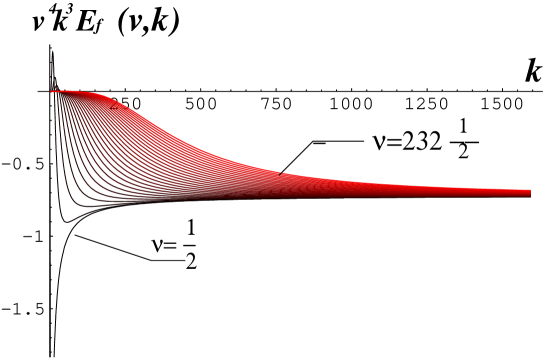
Figure 2: The contribution $E_{f}(\nu,k)$ multiplied by $\nu^{4}k^{3}$ of the individual radial momenta for several orbital momenta to the finite part of the ground state energy for $R_{1}=0.0001$, $R_{2}=1$, $\delta=3$.

Figure 3: The contribution $E_{f}(\nu)$ of the individual orbital momenta to the finite part of the ground state energy multiplied by $\nu^{2}$ for $R_{1}=0.0001$,$R_{2}=1$ and $\delta=3$.

The calculations have been performed for several values of the parameters. The results are displayed in Table.1. The computations are performed with an adapted arithmetical precision. In intermediate steps compensations between sometimes very large quantities appeared. The precision was adapted accordingly. For example, for $R_{1}=0.99,\nu=250.5,k=1600$ as much as 1404 decimal positions have been necessary to get at least 16 digits precision of the integrand $E_{f}(\nu,k)$. This was a factor causing large computation time.

Table 1. The numerical evaluations for several values of $R_{1}$ and $\delta$

$R_{1}$=0.0001
$\delta$ $E^{f}$ $E^{as}$ $E^{ren}$ $E^{class}$ $E^{tot}$ 0.5 -0.0130152 0.00152886 -0.0114863 3.14159 3.13011 1. -0.052403 0.00509591 -0.0473071 12.5664 12.5191 3. -0.450093 -0.052012 -0.502105 113.097 112.595 6. -0.91953 -1.52936 -2.44889 452.389 449.94 10. 4.85954 -12.9483 -8.08871 1256.64 1248.55 15. 46.3333 -67.3661 -21.0328 2827.43 2806.4 21. 215.273 -261.526 -46.2534 5541.77 5495.52 30. 987.62 -1095.29 -107.666 11309.7 11202.1

$R_{1}$=0.9
$\delta$ $E^{f}$ $E^{as}$ $E^{ren}$ $E^{class}$ $E^{tot}$ 0.5 -0.278679 -0.00105651 -0.279736 16.5347 16.255 1. -1.11431 -0.00451479 -1.11882 66.1388 65.02 3. -10.0633 -0.0683525 -10.1317 595.249 585.117 6. -40.4372 -0.647622 -41.0848 2381. 2339.92 10. -112.17 -4.2629 -116.433 6613.88 6497.45 20. -423.279 -63.2506 -486.53 26455.5 25969. 40. -1079.05 -992.187 -2071.24 105822. 103751.

$R_{1}$=0.95
$\delta$ $E^{f}$ $E^{as}$ $E^{ren}$ $E^{class}$ $E^{tot}$ 0.5 -0.72166 -0.00212769 -0.723788 32.2215 31.4977 1. -2.86633 -0.00877711 -2.87511 128.886 126.011 3. -25.8293 -0.104564 -25.9339 1159.97 1134.04 10. -287.834 -4.39364 -292.228 12888.6 12596.4

$R_{1}$=0.99
$\delta$ $E^{f}$ $E^{as}$ $E^{ren}$ $E^{class}$ $E^{tot}$ 0.5 -5.59211 -0.0106385 -5.60275 157.869 152.266 1. -23.2975 -0.0428038 -23.3403 631.476 608.136 3. -202.057 -0.409235 -202.466 5683.28 5480.82

$R_{1}$=0.997
$\delta$ $E^{f}$ $E^{as}$ $E^{ren}$ $E^{class}$ $E^{tot}$ 1. -91.996 -0.142036 -92.138 2097.54 2005.4

$R_{1}$=0.999
$\delta$ $E^{f}$ $E^{as}$ $E^{ren}$ $E^{class}$ $E^{tot}$ 1. -311.182 -0.425555 -311.608 6286.33 5974.72

8 Conclusions and Discussions

In the preceding sections the ground state energy for a spinor in the background of a rectangular shaped flux tube had been numerically calculated. The corresponding Jost function had been written down explicitly, also its asymptotic part. The numerical calculation required work with high arithmetic precision. The results are displayed mainly in Table 1. For small inner radius of the flux the results are close to them of [13] where the same problem for a flux tube with homogeneous magnetic field inside, which corresponds to $R_{1}=0$ here, was considered. Especially, it is seen that for large flux $\delta$ there is a compensation of the $\delta^{4}$-contribution between the finite and the asymptotic parts of the ground state energy leaving a behaviour proportional to $\delta^{2}\ln\delta$ as shown in Fig.4. Here the asymptotic part gave an essential contribution. The ground state energy remains negative, but numerically small. Only for very large flux it could overturn the corresponding classical energy, but these values of the flux are clearly unphysical.

Figure 4: The ground state energy divided by $\delta^{2}\ln\delta$ as function of $\delta$.

For values of the inner radius close to the outer one, $R_{1}\to 1$ (where we have put $R_{2}=1$) the picture changes. Here the vacuum energy grows faster than the classical one. Generally, both diverge proportional to $(1-R_{1})^{-1}$, the classical energy is equal to $E_{\rm class}=\delta^{2}2\pi(1-R_{1})^{-1}$. The vacuum energy, multiplied by $(1-R_{1})$, is shown in Fig.5 in a logarithmic scale. It is negative and growing a bit faster than the classical one which would be a constant in this plot. Here the asymptotic part of the ground state energy becomes increasingly unimportant (see Table 1). The question whether the vacuum energy for sufficiently small $(1-R_{1})$ may become larger than the classical one cannot be answered by the numerical results obtained. The problem is that the computations become very time consuming because of the increasing precision which is required. Also, one has to take higher $k$ and $\nu$ into account. The weakening of the growth for $R_{1}=0.997$ and $R_{1}=0.999$ seen in Fig.5 may be caused just by this reason. Here one has to note that the integrand is for large $k$ and $\nu$ always negative (see Fig.2) so that dropping some part (as we did within the numerical procedure) diminishes the result. So, as a result, we cannot exclude from the given calculation that the vacuum energy grows for a strong background field faster than the classical energy.

Figure 5: The vacuum energy multiplied by $(1-R_{1})$ in a logarithmic scale for $\delta=1$.

Further work is necessary to better understand these questions. An improvement of the numerical procedure is certainly desirable. It could go along two lines. First, in the calculation of the Jost function the compensation of large exponentials should be avoided by taking them into account analytically. Second, in the compensation between the logarithm of the Jost function and its asymptotic expansion in the integrand of $E_{f}$ in Eq.(5.7,5.8) higher orders of the asymptotic expansion could be used. However, for this reason one would have to continue the procedure invented in [13] for this expansion using the Lippman-Schwinger equation or to find some equivalent procedure.

9 Appendix

The sum over $v$ has been transformed to integrals using the Abel-Plana formula as follows:

$$\sum\limits_{l=0}^{\infty}(l+\frac{1}{2})=\int\limits_{0}^{\infty}d\nu f(\nu)+\int\limits_{0}^{\infty}\frac{d\nu}{1+e^{2\pi\nu}}\frac{f(i\nu)-f(i\nu)}{i}$$ (9.1)

The integrations over $\nu$ and $k$ can be done using identities:

$$\int\limits_{0}^{\infty}d\nu\int\limits_{m}^{\infty}dk(k^{2}-m^{2})^{1-s}\frac{\partial}{\partial k}\frac{t^{j}}{\nu^{n}}=-\frac{m^{2-2s}}{2}\frac{\Gamma(2-s)\Gamma(\frac{1+j-n}{2})\Gamma(s+\frac{n-3}{2})}{(rm)^{n-1}\Gamma(\frac{j}{2})}$$ (9.2)

$$\int\limits_{m}^{\infty}dk(k^{2}-m^{2})^{1-s}\frac{\partial}{\partial k}t^{j}=-m^{2-2s}\frac{\Gamma(2-s)\Gamma(s+\frac{j}{2}-1)}{\Gamma(\frac{j}{2})}\frac{(\frac{\nu}{rm})^{j}}{(1+(\frac{\nu}{rm})^{2})^{s+\frac{j}{2}-1}}$$ (9.3)

The expansion in powers of $\nu$ for logarithm of asymptotic Jost function can be obtained in the form (see[9])

$$ln\boldmath f_{as}\unboldmath(ik)=\sum\limits_{n=1}^{3}\sum\limits_{j=1}^{9}\int\limits_{0}^{\infty}\frac{dr}{r}X_{nj}\frac{t^{j}}{\nu^{n}}\\$$ (9.4)

where
$X_{1,1}=-X_{1,3}=X_{2,6}=\frac{1}{2}(a\delta)^{2}\\$
$X_{2,2}=\frac{1}{4}\delta^{2}(a^{2}-raa^{\prime})\\$
$X_{2,4}=\frac{1}{4}\delta^{2}(-3a^{2}+raa^{\prime})\\$
$X_{3,3}=\frac{1}{4}\delta^{2}(a^{2}-raa^{\prime}+\frac{1}{2}r^{2}aa^{\prime\prime}-\frac{1}{2}\delta^{2}a^{4})\\$
$X_{3,5}=\frac{1}{8}\delta^{2}(-\frac{39}{2}a^{2}+7raa^{\prime}-r^{2}aa^{\prime\prime}+6\delta^{2}a^{4})\\$
$X_{3,7}=\frac{1}{8}\delta^{2}(35a^{2}-5raa^{\prime}-5\delta^{2}a^{4})\\$
$X_{3,9}=\frac{-35}{16}\delta^{2}a^{2}\\$

For the representation of $E_{as}$ as 5.6

$$E^{as}=\frac{-4}{\pi}\int\limits_{0}^{\infty}\frac{dr}{r^{3}}[\delta^{2}a(r)^{2}g_{1}(rm)-\delta^{2}r^{2}a^{\prime}(r)^{2}g_{2}(rm)+\delta^{4}a(r)^{4}g_{3}(rm)]\\$$ (9.5)

here $f_{i}$ are

$$f_{1}(x) = \frac{1}{2}f_{1,1}(x)-\frac{1}{2}f_{1,3}(x)+\frac{1}{4}f_{3,3}-\frac{39}{16}f_{3,5}(x)+\frac{35}{8}f_{3,7}(x)-\frac{35}{16}f_{3,9}(x)$$

$$- \frac{1}{2}x\partial_{x}(-\frac{1}{4}f_{3,3}(x)+\frac{7}{8}f_{3,5}(x)-\frac{5}{8}f_{3,7}(x))$$

$$+ \frac{1}{2}x\partial_{x}^{2}(\frac{x}{8}f_{3,3}(x)-\frac{x}{8}f_{3,5}(x)),$$

$$f_{2}(x) = \frac{1}{8}(f_{3,3}(x)-f_{3,5}(x)),$$

$$f_{3}(x) = -\frac{1}{8}(f_{3,3}(x)-6f_{3,5}(x)+5f_{3,7}(x)).$$ (9.6)

with $f_{i.j}$ are

$$f_{1,1}(x) = -\frac{1}{1+e^{2\pi x}}$$

$$f_{1,3}(x) = -(\frac{}{1+e^{2\pi x}})^{\prime}$$

$$f_{3,3}(x) = (\frac{1}{x}\frac{1}{1+e^{2\pi x}})^{\prime}$$

$$f_{3,5}(x) = \frac{1}{3}(\frac{1}{x}(\frac{x}{1+e^{2\pi x}})^{\prime})^{\prime}$$

$$f_{3,7}(x) = \frac{1}{15}(\frac{1}{x}(\frac{1}{x}(\frac{x^{3}}{1+e^{2\pi x}})^{\prime})^{\prime})^{\prime}$$

$$f_{3,9}(x) = \frac{1}{105}(\frac{1}{x}(\frac{1}{x}(\frac{1}{x}(\frac{x^{5}}{1+e^{2\pi x}})^{\prime})^{\prime})^{\prime})^{\prime}$$ (9.7)

The asymtotic of the logarithmic Jost function can be obtained in the form: $\ln f_{\nu}(ik)=\sum\limits_{n}h_{n}(t_{1},t_{2})$,(see 6.4) with:

$$h_{1} = \frac{4}{3}\lambda^{2}[{R_{1}}^{4}t_{1}(2+t_{1}){(1+t_{2})}^{2}-3{R_{1}}^{2}{R_{2}}^{2}{(1+t_{1})}^{2}t_{2}(1+t_{2})+{R_{2}}^{4}{(1+t_{1})}^{2}t_{2}(1+2t_{2})]$$

$$h_{2} = 0$$

$$h_{3} = -\frac{1}{6}{\lambda}^{2}[2{R_{1}}^{4}{t_{1}}^{3}{(1+t_{2})}^{2}+{R_{1}}^{2}{R_{2}}^{2}{(1+t_{1})}^{2}{t_{2}}^{3}{(1+t_{2})}^{2}(3{t_{2}}^{2}-4)-$$

$${R_{2}}^{4}{(1+t_{1})}^{2}{t_{2}}^{3}(3{t_{2}}^{4}+6{t_{2}}^{3}-{t_{2}}^{2}-8t_{2}-2)]+$$

$$\frac{2}{15}{\lambda}^{4}[4{R_{1}}^{8}{t_{1}}^{3}(4+t_{1}){(1+t_{2})}^{4}-5{R_{1}}^{6}{R_{2}}^{2}{(1+t_{1})}^{4}{t_{2}}^{3}{(1+t_{2})}^{4}+$$

$$15{R_{1}}^{4}{R_{2}}^{4}{(1+t_{1})}^{4}{t_{2}}^{3}{(1+t_{2})}^{2}({t_{2}}^{2}+2t_{2}-1)-$$

$$5{R_{1}}^{2}{R_{2}}^{6}{(1+t_{1})}^{4}{t_{2}}^{3}(3{t_{2}}^{4}+12{t_{2}}^{3}+6{t_{2}}^{2}-4t_{2}-1)+$$

$${R_{2}}^{8}{(1+t_{1})}^{4}{t_{2}}^{3}(5{t_{2}}^{4}+20{t_{2}}^{3}-4t_{2}-1)]$$

$$h_{4} = \frac{\delta^{2}[{R_{1}}^{4}{t_{1}}^{4}(1-{t_{1}}^{2})+{R_{2}}^{4}{t_{2}}^{4}(1-{t_{2}}^{2})]}{4{(R_{1}^{2}-R_{2}^{2})}^{2}}$$

$$\lambda = \frac{\delta}{(R_{1}^{2}-R_{2}^{2})(1+t_{1})(1+t_{2})}$$ (9.8)

References

[1]
H.B.G. Casimir, Proc. Kon. Ned. Akad. Wetensch.51, 793 (1948).
[2]
M. Bordag, U. Mohideen, and V. M. Mostepanenko.
New developments in the Casimir effect.
Phys. Rep.353 1, (2001).
[3]
V.M. Mostepanenko and N.N. Trunov, The Casimir Effect and its
Applications, Clarendon Press, Oxford, (1997).
[4]
K. A. Milton, The Casimir effect: Physical manifestations of
zero-point energy, River Edge, USA: World Scientific (2001).
[5]
W. Heisenberg, H. Euler, Z.Phys.98, 714 (1936).
[6]
Martin Groves and Warren B. Perkins.
The Dirac sea contribution to the energy of an electroweak string.
Nucl. Phys.B 573, 449 (2000).
[7]
Dmitri Diakonov and Martin Maul.
Center-vortex solutions of the Yang-Mills effective action in three
and four dimensions,
(hep-lat/0204012).
[8]
G. Dunne and T. M. Hall, An exact QED 3+1 effective action, Phys. Lett.B 419, 322 (1998).
[9]
M. Bordag and K. Kirsten, The ground state energy of a spinor field in the
background of a finite radius flux tube, Phys. Rev.D 60, 105019 (1999)
[10] M.Fry,Int.J.Mod.Phys.A17, 936 (2002) and references therein.
[11]
Marco Scandurra.
Vacuum energy in the presence of a magnetic string with delta
function profile.
Phys. Rev., D62, 085024 (2000).
[12]
Ana Achucarro and Tanmay Vachaspati.
Semilocal and electroweak strings.
Phys. Rept.327, 347 (2000).
[13] M. Bordag and K. Kirsten, Vacuum energy in a
spherically symmetric background field., Phys. Rev. D 53, 5753
(1996)
[14]
Y.Aharonov and A.Casher, Ground state of a spin-1/2 charged particle in a
two-dimensional magnetic field,Phys.Rev.A 19, 2461 (1979).
[15]
M. Bordag, E. Elizalde, and K. Kirsten.
Heat kernel coefficients of the Laplace operator on the D-
dimensional ball.,
J. Math. Phys.37, 895 (1996).
[16]
K. Kirsten, Spectral Functions in Mathematics and
Physics, Chapman & Hall/CRC, Boca Raton, FL (2001).
[17]
P. B. Gilkey, Invariance Theory, the heat equation and the Atyah-Singer index theorem, Publish or Perish, Wilmington, Delaware (1984).
[18]
P. B. Gilkey, K. Kirsten and D. V. Vassilevich, Heat trace asymptotics with transmittal boundary conditions and quantum brane-world scenario,
Nucl. Phys.B 601, 125 (2001).
[19]
M. Bordag, E. Elizalde, K. Kirsten, and S. Leseduarte.
Casimir energies for massive fields in the bag.
Phys. Rev., D 56, 4896 (1997).
[20]
M. Bordag, A. S. Goldhaber, P. van Nieuwenhuizen and D. Vassilevich,
Heat kernels and zeta-function regularization for the mass of the SUSY kink,
(hep-th/0203066).
[21]
M. Bordag, K. Kirsten and D. Vassilevich,
On the ground state energy for a penetrable sphere and for a dielectric ball,
Phys. Rev.D 59, 085011 (1999).
[22] M. Bordag, Vacuum energy in smooth background
fields, J. Phys. A: Math. Gen.28, 755 (1995).
[23]
M. Bordag and S. G. Voropaev, Bound states of an electron in the field of
the magnetic string, Phys. Lett.B 333, 238 (1994).
[24] M. Abramovitz and I. A. Stegun, Handbook of
Mathematical Functions, Natl. Bur. Stand. Appl. Math. Ser. 55,
Washington, D. C. :US GPO, New York:Dover, reprinted (1972).
[25] I. S. Gradshteyn and I. M. Ryzhik, Tables of
integrals, series and products; Academic Press, Inc. 5th ed. (1965).
[26]
M. Bordag and D. V. Vassilevich.
Heat kernel expansion for semitransparent boundaries,
J. Phys. A., 32 8247 (1999).
[27]
Ian G Moss.
Heat kernel expansions for distributional backgrounds,
Phys. Lett.,B491, 203 (2000).
[28]
Peter Gilkey, Klaus Kirsten, and Dmitri Vassilevich.
Heat trace asymptotics defined by transfer boundary
conditions, (hep-th/0208130).
[29] E. Elizalde, M. Bordag and K. Kirsten, Casimir energy
for a massive fermionic quantum field with a spherical boundary, J. Phys. A:Math. Gen.31, 1743 (1998).
[30]
Marco Scandurra.
Vacuum energy of a massive scalar field in the presence of a
semi-transparent cylinder,
J. Phys.A33, 5707 (2000).