ICOSAHEDRAL SKYRMIONS

Abstract

In this paper we aim to determine the baryon numbers at which the minimal energy Skyrmion has icosahedral symmetry. By comparing polyhedra which arise as minimal energy Skyrmions with the dual of polyhedra that minimize the energy of Coulomb charges on a sphere, we are led to conjecture a sequence of magic baryon numbers, $B=7,17,37,67,97,...$ at which the minimal energy Skyrmion has icosahedral symmetry and unusually low energy. We present evidence for this conjecture by applying a simulated annealing algorithm to compute energy minimizing rational maps for all degrees upto 40. Further evidence is provided by the explicit construction of icosahedrally symmetric rational maps of degrees 37, 47, 67 and 97. To calculate these maps we introduce two new methods for computing rational maps with Platonic symmetries.

1 Introduction

Skyrmions are topological solitons in three space dimensions which are candidates for an effective description of nuclei, with an identification between soliton and baryon numbers [10]. Recently, the minimal energy Skyrmions for all baryon numbers $1\leq B\leq 22$ were computed and their symmetries identified [3]. The baryon density of these Skyrmions is localized around the vertices and edges of polyhedra, which are almost always trivalent, and for $B\geq 7$ are composed of 12 pentagons and $2B-14$ hexagons, with only a few exceptions (which can be understood by a symmetry enhancement principle). These Skyrmions have discrete point group symmetries, including occasional Platonic symmetries. For $B=7$ and $B=17$ the minimal energy Skyrmion is particularly symmetric, having icosahedral symmetry $Y_{h}$, and the value of the energy is unusually low. However, there are other baryon numbers at which icosahedral Skyrme fields exist, but the minimal energy Skyrmion has less symmetry. This motivates the main question addressed in this paper, namely, what are the magic baryon numbers at which the minimal energy Skyrmion has icosahedral symmetry with a resulting unusually low energy?

To gain some insight into this problem we note that, as first observed in [2], there is a close relationship between the polyhedra which arise as minimal energy Skyrmions and the duals of polyhedra which occur in the problem of minimizing point Coulomb charges on a sphere. This latter problem is often known as the Thomson problem, even though he appears not to have posed it explicitly, and we shall use this nomenclature here. The Thomson problem is well studied for upto 200 points on the sphere [9] and generically the $n$ points sit at the vertices of a combinatoric deltahedron. Taking the dual of a deltahedron leads to a trivalent polyhedron, which is the class of polyhedra which generically arise for Skyrmions. A Skyrmion polyhedron with baryon number $B$ has $2B-2$ faces, so to identify this with the dual of a Thomson polyhedron requires that we consider $n=2B-2$ Coulomb charges on the sphere. Let us denote by $G_{B}$ the symmetry of the minimal energy Skyrmion with baryon number $B$ and by $H_{B}$ the symmetry of the minimal energy Thomson configuration of $2B-2$ points on the sphere. Extracting the information from references [3] and [5] we obtain Table 1, in which we compare the symmetries of the minimal energy configurations for each problem.

From Table 1 it is clear that although a variety of different Platonic, dihedral and cyclic symmetry groups occur, there is a remarkable match for the two problems in 17 out of the 22 cases. Moreover, a closer inspection reveals that in these 17 cases not only do the symmetry groups match, but the combinatorial types of the Skyrmion polyhedron and the dual of the Thomson polyhedron are identical. The five examples that do not coincide, $B=5,9,10,19,22$ shows that the topography of the two energy functions is slightly different and suggests that the same factors which determine the polyhedron (or its dual) are important, but perhaps with slightly different weightings. For example, for $B=9$ and $B=10$, which are not particularly low in energy, it is known that Skyrmion configurations exist which have the symmetries required to match to those of the Thomson problem, but that they have very slightly higher energy than the minimal energy Skyrmion. The fact that there is so often an agreement for the two problems leads us to believe that, in the cases where particularly symmetric low energy configurations arise, they will be the minima in both problems. Thus, as a working hypothesis to test, we shall postulate that $G_{B}$ is the icosahedral group only if $H_{B}$ is also the icosahedral group.

$B$	1	2	3	4	5	6	7	8	9	10	11	12	13	14	15	16	17	18	19	20	21	22
$G_{B}$	$O(3)$	$D_{\infty h}$	$T_{d}$	$O_{h}$	$D_{2d}$	$D_{4d}$	$Y_{h}$	$D_{6d}$	$D_{4d}$	$D_{3}$	$D_{3h}$	$T_{d}$	$O$	$C_{2}$	$T$	$D_{2}$	$Y_{h}$	$D_{2}$	$D_{3}$	$D_{6d}$	$T_{d}$	$D_{3}$
$H_{B}$	$O(3)$	$D_{\infty h}$	$T_{d}$	$O_{h}$	$D_{4d}$	$D_{4d}$	$Y_{h}$	$D_{6d}$	$T$	$D_{4d}$	$D_{3h}$	$T_{d}$	$O$	$C_{2}$	$T$	$D_{2}$	$Y_{h}$	$D_{2}$	$D_{2}$	$D_{6d}$	$T_{d}$	$D_{5h}$

Table 1: The symmetry group $G_{B}$ of the minimal energy Skyrmion with baryon number $B$ and the symmetry group $H_{B}$ of the $2B-2$ points which minimize the Thomson problem.

Although the Thomson problem is a difficult one to study numerically, it is certainly much easier than finding minimal energy Skyrmions, so we can take advantage of the known numerical results. Minimal energy configurations are currently available for upto 200 points, that is, $B\leq 101$, and of these the values $B=7,17,37,62,67,97$ are selected as magic numbers at which the configuration has icosahedral symmetry and unusually low energy when compared to a numerical fit of all 200 configurations [9]. As we describe later, the case $B=62$ is rather different from the others in the sequence, so we shall leave this example out for the moment. We are thus led to conjecture that there is a sequence $B=7,17,37,67,97,...$ at which the minimal energy Skyrmion has icosahedral symmetry and unusually low energy. In the rest of this paper we perform some investigations to test this conjecture, and hence the connection between Skyrmions and the Thomson problem.

2 Minimizing Rational Maps

A static Skyrme field, $U({\bf x}),$ is an $SU(2)$ matrix defined throughout $\hbox{\mybb R}^{3}$ and satisfying the boundary condition that $U\rightarrow 1$ as $|{\bf x}|\rightarrow\infty.$ This boundary condition implies a compactification of space so that the Skyrme field becomes a mapping $U:S^{3}\mapsto SU(2),$ and so can be classified by an integer valued winding number

$$B=\frac{1}{24\pi^{2}}\int\epsilon_{ijk}\,\mbox{Tr}\left(\partial_{i}U\,U^{-1}\partial_{j}U\,U^{-1}\partial_{k}U\,U^{-1}\right)d^{3}x,$$ (2.1)

which is a topological invariant. This winding number counts the number of solitons in a given field configuration and is identified with baryon number in the application to modelling nuclei.

The energy of a static Skyrme field is given by

$$E=\frac{1}{12\pi^{2}}\int\mbox{Tr}\left(-\frac{1}{2}\left(\partial_{i}U\,U^{-1}\right)^{2}-\frac{1}{16}\left[\partial_{i}U\,U^{-1},\;\partial_{j}U\,U^{-1}\right]^{2}\right)d^{3}x$$ (2.2)

and for each integer $B,$ the problem is to minimize this energy within the class of fields with baryon number $B$ in order to find the minimal energy Skyrmion. This problem has been solved numerically for all $B\leq 22$ [3] yielding the results presented in Table 1 for the symmetries of the minimal energy Skyrmions. When we refer to the symmetry of a Skyrmion we do not mean that the Skyrme field itself is invariant under particular spatial rotations, but rather that the effect of a spatial rotation can be undone by the application of the global $SO(3)$ symmetry of the Skyrme model, which acts through the conjugation $U\mapsto{\cal O}U{\cal O}^{\dagger},$ where ${\cal O}\in SU(2)$ is a constant matrix. In particular this means that the baryon and energy densities (the integrands in (2.1) and (2.2)) are strictly invariant.

It is computationally prohibitive to apply the full numerical scheme to larger values of $B$ at the present time, but fortunately an approximation method has been developed which provides very accurate results. This is the rational map ansatz [7], where a Skyrme field with baryon number $B$ is constructed from a degree $B$ rational map between Riemann spheres. Although this ansatz does not give exact solutions of the static Skyrme equations, it produces approximations which have energies only a few percent above the numerically computed solutions. Briefly, use spherical coordinates in $\hbox{\mybb R}^{3}$, so that a point ${\bf x}\in\hbox{\mybb R}^{3}$ is given by a pair $(r,z)$, where $r=|{\bf x}|$ is the distance from the origin, and $z$ is a Riemann sphere coordinate giving the point on the unit two-sphere which intersects the half-line through the origin and the point ${\bf x}$. Now, let $R(z)$ be a degree $B$ rational map between Riemann spheres, that is, $R=p/q$ where $p$ and $q$ are polynomials in $z$ such that $\max[\mbox{deg}(p),\mbox{deg}(q)]=B$, and $p$ and $q$ have no common factors. Given such a rational map the ansatz for the Skyrme field is

$$U(r,z)=\exp\bigg{[}\frac{if(r)}{1+|R|^{2}}\pmatrix{1-|R|^{2}&2\bar{R}\cr 2R&|R|^{2}-1\cr}\bigg{]}\,,$$ (2.3)

where $f(r)$ is a real profile function satisfying the boundary conditions $f(0)=\pi$ and $f(\infty)=0$, which is determined by minimization of the Skyrme energy of the field (2.3) given a particular rational map $R$.

Substitution of the rational map ansatz (2.3) into the Skyrme energy functional results in the following expression for the energy

$$E=\frac{1}{3\pi}\int\bigg{(}r^{2}f^{\prime 2}+2B(f^{\prime 2}+1)\sin^{2}f+{\cal I}\frac{\sin^{4}f}{r^{2}}\bigg{)}\ dr\,,$$ (2.4)

where ${\cal I}$ denotes the integral

$${\cal I}=\frac{1}{4\pi}\int\bigg{(}\frac{1+|z|^{2}}{1+|R|^{2}}\bigg{|}\frac{dR}{dz}\bigg{|}\bigg{)}^{4}\frac{2i\ dzd\bar{z}}{(1+|z|^{2})^{2}}\,.$$ (2.5)

To minimize the energy (2.4) one first determines the rational map which minimizes ${\cal I}$, then given the minimum value of ${\cal I}$ it is a simple exercise to find the minimizing profile function. Thus, within the rational map ansatz, the problem of finding the minimal energy Skyrmion reduces to the simpler problem of calculating the rational map which minimizes the function ${\cal I}$.

The baryon density of the rational map $R=p/q$ is proportional to the Wronskian

$$w(p,q)=p^{\prime}q-q^{\prime}p$$ (2.6)

which has $2B-2$ roots, giving the points on the Riemann sphere for which the baryon density vanishes along the corresponding half-lines through the origin. These $2B-2$ points on the sphere give the face-centres of the Skyrmion polyhedron, or equivalently the vertices of the dual polyhedron which is associated with the Thomson problem.

Using a simulated annealing algorithm the ${\cal I}$ minimizing rational maps for $1\leq B\leq 22$ have been computed [3] and found to be in good agreement with the results of full Skyrme field minimization. Here we extend the simulated annealing computation to $B\leq 40,$ in an attempt to determine particularly low energy magic numbers. In the Thomson problem the magic numbers are determined by comparing the energy of minimal solutions with the energy of a numerical fit to the data of all known minimal energy solutions - thereby isolating cases where the energy is lower than the expected fit. In the problem of minimizing rational maps it turns out that there is a more natural approach, due to the fact that a useful lower bound exists. Using a simple inequality it is shown in [7] that ${\cal I}\geq B^{2}.$ It turns out that examining the excess above this bound, by computing the quantity ${\cal I}/B^{2}$, is a good diagnostic tool for highlighting low energy maps, and in particular is more useful than simply calculating the energy of the associated Skyrme field. We illustrate this in Fig. 1 by plotting ${\cal I}/B^{2}$ for the results of our simulated annealing computations for $2\leq B\leq 40.$

Figure 1: ${\cal I}/B^{2}$ for $2\leq B\leq 40,$ as calculated by ${\cal I}$ minimizing simulated annealing computations. Also shown are the values of ${\cal I}/B^{2}$ for the icosahedrally symmetric Skyrmions with $B=47$ (cross), $B=67$ (square) and $B=97$ (circle), discussed in the text.

There are clear dips at the magic numbers $B=7$ and $B=17,$ corresponding to the already known low energy icosahedral Skyrmions (see Table 1). There are also dips at $B=4$ and $B=13$, where it is known that the Skyrmions also have Platonic symmetry, but this time octahedral (see Table 1). However, there is one more major dip at $B=37,$ and this is precisely the value predicted as the next magic number in the icosahedral sequence suggested by comparison with the Thomson problem. This result, therefore, provides strong support for our conjectured sequence, providing we can prove that this low energy degree 37 map obtained from simulated annealing does indeed have icosahedral symmetry. This will be discussed in the next section.

Note that the quantity ${\cal I}/B^{2}$ appears to be tending towards an asymptotic value of around $1.28,$ apart from magic numbers where it drops to around $1.25.$ It would be interesting to understand this approach to a relatively constant value, as well as its magnitude.

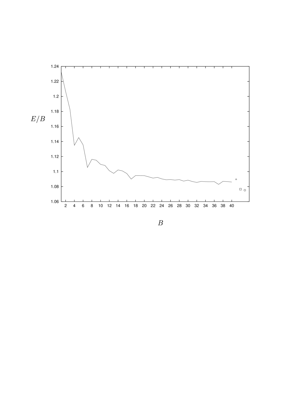
Figure 2: The energy per baryon $E/B$ of the Skyrmions constructed from the minimizing maps with $1\leq B\leq 40.$ Also shown are the values of $E/B$ for the icosahedrally symmetric Skyrmions with $B=47$ (cross), $B=67$ (square) and $B=97$ (circle), discussed in the text.

In Fig. 2 we plot the energy per baryon $E/B$ of the Skyrmions constructed from the minimizing maps with $1\leq B\leq 40.$ The dips at the magic numbers are clearly visible in Fig. 2, reproducing the sequence displayed in Fig. 1. However, in this case the dips are superimposed upon a general decrease of $E/B$ with increasing $B,$ which is why we regard the quantity ${\cal I}/B^{2}$ as a more useful diagnostic than $E/B.$

The radius of a Skyrmion produced from the rational map ansatz can be defined as the radial value, $r_{*},$ at which the profile function is equal to $\pi/2.$ In Fig. 3 we plot $r_{*}^{2}$ as a function of $B$ for $1\leq B\leq 40.$ This clearly shows that the radius has a $\sqrt{B}$ dependence, and given that all these configurations are reasonably close to the Faddeev-Bogomolny energy bound $E\geq|B|$, this means that the energy grows like the square of the radius, as expected for a shell-like structure. Note that at the magic numbers the radius of the Skyrmion is slightly less than expected, presumably due to a more compact arrangement of a particularly symmetric energy density.

Figure 3: $r_{*}^{2},$ the squared radius of the Skyrmion, as a function of baryon number $B.$

3 Computing Icosahedral Maps

Recall that a Skyrmion is symmetric under a group $G\subset SO(3),$ if a spatial rotation $g\in SO(3)$ can be compensated by an action of the global $SO(3)$ symmetry. In terms of the rational map approach a spatial rotation acts on the Riemann sphere coordinate $z$ as an $SU(2)$ Möbius transformation. Similarly the global symmetry acts as on the Riemann sphere coordinate $R$ of the target 2-sphere as an $SU(2)$ Möbius transformation. Hence, a map is $G$-symmetric if, for each $g\in G$, there exists a target space rotation $D_{g}$ such that $R(g(z))=D_{g}(R(z)).$ Since we are dealing with $SU(2)$ transformations the set of target space rotations will form a representation of the double group of $G$, but we shall continue to call this $G.$

To determine the existence and compute particular symmetric rational maps is a matter of classical group theory. We are concerned with degree $B$ polynomials which form the carrier space for $\underline{B+1}$, the $(B+1)$-dimensional irreducible representation of $SU(2).$ Now, as a representation of $SU(2)$ this is irreducible, but if we only consider the restriction to a subgroup $G$, $\underline{B+1}|_{G}$, this will in general be reducible. What we are interested in is the irreducible decomposition of this representation and tables of these subductions can be found, for example, in ref. [1].

The simplest case in which a $G$-symmetric degree $B$ rational map exists is if

$$\underline{B+1}|_{G}=E+...$$ (3.1)

where $E$ denotes a two-dimensional representation. Here, and in the following, the dots denote representations of dimension higher than those shown. In this case a basis for $E$ consists of two degree $B$ polynomials which can be taken to be the numerator and denominator of the rational map. A subtle point which needs to be addressed is that the two basis polynomials may have a common root, in which case the resulting rational map is degenerate and does not correspond to a genuine degree $B$ map.

More complicated situations can arise, for example, if

$$\underline{B+1}|_{G}=A_{1}+A_{2}+...$$ (3.2)

where $A_{1}$ and $A_{2}$ denote two one-dimensional representations, then a whole one-parameter family of maps can be obtained by taking a constant multiple of the ratio of the two polynomials which are a basis for $A_{1}$ and $A_{2}$ respectively. An $m$-parameter family of $G$-symmetric maps can be constructed if the decomposition contains $(m+1)$ copies of a two-dimensional representation, that is,

$$\underline{B+1}|_{G}=(m+1)E+...$$ (3.3)

where the $m$ (complex) parameters correspond to the freedom in the choice of one copy of $E$ from $(m+1)E.$

A detailed explanation of how to explicitly calculate any required symmetric map is given in [7]. However, this approach involves computing appropriate projectors which are matrices of size $(B+1)\times(B+1),$ and even with the use of symbolic computational packages this procedure becomes cumbersome for the large values of $B$ that we are interested in here. In this section we therefore describe and apply two new, more convenient, methods for calculating symmetric maps. We shall concentrate on the situation of relevance to this paper, where $G=Y,$ the icosahedral group, but the methods are applicable for any $G.$

Before we describe our new approaches we need to recall some facts about representations of the icosahedral group and Klein polynomials of the icosahedron. The icosahedral group $Y$ has the trivial 1-dimensional representation $A$ and two 2-dimensional representations, which we denote by $E_{1}^{\prime}$ and $E_{2}^{\prime},$ with a prime denoting the fact that these are representations of the double group of $Y$ which are not representations of $Y.$ There are also three, four, five and six-dimensional representations, but we shall not need these here.

Klein polynomials are strictly invariant polynomials for the Platonic groups [8]. Since,

$$\underline{13}|_{Y}=A+...$$ (3.4)

this implies that there is degree 12 invariant polynomial. This is the Klein polynomial given by

$$k_{v}=z^{11}+11z^{6}-z$$ (3.5)

and although it appears to have degree 11, it should be thought of as having degree 12 with one root at infinity. The roots of this polynomial, considered as points on the Riemann sphere, are located at the vertices of a suitably oriented and scaled icosahedron. The same construction, but using the face-centres and mid-points of the edges of the icosahedron, in place of the vertices, produces the Klein polynomials

$$k_{f} = z^{20}-228z^{15}+494z^{10}+228z^{5}+1$$ (3.6)

$$k_{e} = z^{30}+522z^{25}-10005z^{20}-10005z^{10}-522z^{5}+1$$ (3.7)

which are also $Y$-invariant, by construction.

3.1 Polarization

In this subsection we describe our polarization method for computing symmetric maps. It has similar features to the polarization technique used to construct symmetric Nahm data [6].

Suppose we wish to obtain the symmetric degree $B$ map associated with the decomposition

$$\underline{B+1}|_{Y}=E+...$$ (3.8)

where $E$ denotes one of the 2-dimensional representations. The above fact implies that

$$E\otimes\underline{B+1}|_{Y}=A+...$$ (3.9)

and, in our polarization method, the invariant polynomial corresponding to this 1-dimensional representation is used to construct a basis for the $E$ in (3.8).

It is convenient to work with homogeneous coordinates $x,y$ on the Riemann sphere, that is, $z=x/y$, so that a polynomial in $z$ of degree $B$ corresponds to a homogeneous degree $B$ polynomial in $x$ and $y.$

Let $(p_{L}(x,y),q_{L}(x,y))$ be known degree $L$ polynomials which form a basis for the representation $E$ and let $k(x,y)$ be a degree $B+L$ invariant polynomial which is a basis for the 1-dimensional representation in (3.9). Then, since the pair $(\partial_{y},-\partial_{x})$ transform in the same way as the pair $(x,y)$ under linear $SU(2)$ transformations, this means that the polynomials $p_{B}(x,y),q_{B}(x,y)$ defined by

$$p_{B}(x,y)=p_{L}(\partial_{y},-\partial_{x})k(x,y),\quad q_{B}(x,y)=q_{L}(\partial_{y},-\partial_{x})k(x,y)$$ (3.10)

have degree $B$ and are the required basis for the 2-dimensional representation occuring in (3.8).

As an example of this scheme we now construct the icosahedrally symmetric degree 17 rational map, in an orientation that we shall require later. The relevant decomposition is

$$\underline{18}|_{Y}=E_{2}^{\prime}+...$$ (3.11)

so we first require a known $Y$-symmetric rational map that is a basis for the representation $E_{2}^{\prime}.$ The simplest known example is the degree 7 map [7] (corresponding to the $B=7$ $Y_{h}$-symmetric minimal energy Skyrmion)

$$p_{7}(x,y)=x^{7}-7x^{5}y^{2}-7x^{2}y^{5}-y^{7},\quad q_{7}(x,y)=x^{7}+7x^{5}y^{2}-7x^{2}y^{5}+y^{7}.$$ (3.12)

Hence we have $B=17$ and $L=7,$ so now we require an invariant polynomial $k(x,y)$ of degree $B+L=24.$ This is easily found by using an appropriate combination of Klein polynomials, in this case $k(x,y)=k_{v}^{2}(x,y)$ is the degree 24 invariant where $k_{v}(x,y)=x^{11}y+11x^{6}y^{6}-xy^{11}$ is the degree 12 Klein polynomial given earlier, when written in terms of homogeneous coordinates. The formula (3.10) then produces

$$p_{17} = z^{17}+17z^{15}+119z^{12}-187z^{10}+187z^{7}+119z^{5}+17z^{2}-1$$

$$q_{17} = z^{17}-17z^{15}+119z^{12}+187z^{10}+187z^{7}-119z^{5}+17z^{2}+1$$ (3.13)

when written in terms of the inhomogeneous coordinate $z.$ This map is equivalent, after a change of spatial and internal orientation, to the $Y_{h}$-symmetric map presented in [7] that corresponds to the $B=17$ $Y_{h}$-symmetric minimal energy Skyrmion. In the following subsection we shall require this map in the orientation presented in (3.13).

Although this method is much easier to implement than the projector algorithm, it turns out that for the icosahedral maps we require in this paper there is yet another approach, which is even more effecient.

3.2 Klein Leapfrog

From the previous section we already have two $Y$-symmetric rational maps, which are $R_{7}=p_{7}/q_{7}$ and $R_{17}=p_{17}/q_{17}.$ Here we describe how the other $Y$-symmetric maps that we require can be obtained from these two by the simple multiplication of invariant Klein polynomials. This way of obtaining higher degree invariant rational maps we refer to as the Klein Leapfrog method.

Recall that we wish to determine whether the low energy ${\cal I}$ minimizing map of degree 37 that we found earlier is icosahedrally symmetric. The relevant decomposition is

$$\underline{38}|_{Y}=E_{1}^{\prime}+2E_{2}^{\prime}+...$$ (3.14)

Both the maps $(p_{7},q_{7})$ and $(p_{17},q_{17})$ are a basis for the representation $E_{2}^{\prime}$, and the multiplication of these maps by any (integer power of a) Klein polynomial does not change the transformation properties, since Klein polynomials are invariants. Thus, both $(k_{e}p_{7},k_{e}q_{7})$ and $(k_{f}p_{17},k_{f}q_{17})$ are degree 37 $Y$-symmetric maps. Each map alone is not a valid degree 37 rational map, since the numerator and denominator contain common factors, but taken together they form an acceptable basis for the $2E_{2}^{\prime}$ in (3.14). Explicitly,

$$R_{37}=\frac{p_{37}}{q_{37}}=\frac{k_{f}p_{17}+ck_{e}p_{7}}{k_{f}q_{17}+ck_{e}q_{7}}$$ (3.15)

where $c$ is a complex parameter. For $c=0$ or $c=\infty$ the map is clearly degenerate, having degree lower than 37, but for generic values of $c$ the numerator and denominator are coprime.

The Wronskian of this map must be strictly invariant, and indeed it is given by the following combination of Klein polynomials

$$w(p_{37},q_{37})=k_{e}^{2}k_{v}(80c+28c^{2})-k_{f}^{3}k_{v}(68+120c).$$ (3.16)

The 72 roots of this polynomial give the face-centres of the Skyrmion polyhedron. Minimizing the integral ${\cal I}$ over the one (complex) parameter family of maps (3.15) results in a minimum at $c=-0.829+0.545i,$ where ${\cal I}/B^{2}=1.255.$ This is precisely the value found by the minimization over all degree 37 maps, so we confirm that the ${\cal I}$ minimizing degree 37 map, and hence the minimal energy $B=37$ Skyrmion, has icosahedral symmetry. Note that the symmetry group is only $Y$ and not $Y_{h}$ since $c$ is not real. A baryon density isosurface plot for the associated Skyrmion is displayed in Fig. 4a.

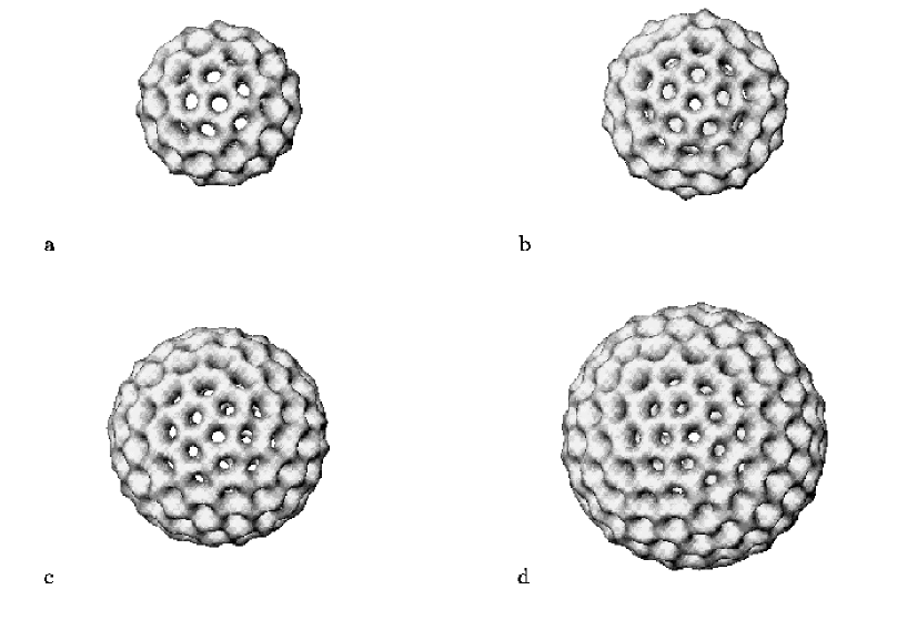
Figure 4: Baryon density isosurface plots (to scale) for icosahedral Skyrmions with baryon numbers a) $B=37$, b) $B=47$, c) $B=67$, d) $B=97$.

The next magic number in our conjectured icosahedral list is $B=67.$ The application of our simulated annealing scheme to extend the results presented in Fig. 1 to such a large value of $B$ would require unreasonable computing resources. We therefore make use of the fact that the quantity ${\cal I}/B^{2}$ appears to approach an asymptotic value of around $1.28,$ whereas for icosahedral magic numbers the value is closer to $1.25.$ Therefore we aim to present evidence in support of our conjecture by finding an icosahedral map of degree 67 with ${\cal I}/B^{2}\approx 1.25.$

The relevant decomposition is

$$\underline{68}|_{Y}=2E_{1}^{\prime}+3E_{2}^{\prime}+...$$ (3.17)

so we require three degree 67 maps to form a basis for the second component in the above decomposition. These are given by a Klein leapfrog as

$$(k_{e}k_{f}p_{17},k_{e}k_{f}q_{17}),\quad(k_{e}^{2}p_{7},k_{e}^{2}q_{7}),\quad(k_{f}^{3}p_{7},k_{f}^{3}q_{7}).$$ (3.18)

It might seem strange that $(k_{v}^{5}p_{7},k_{v}^{5}q_{7})$ is not included, but because $\underline{61}|_{Y}=2A+...,$ there must be a linear relationship between $k_{e}^{2}$, $k_{f}^{3}$ and $k_{v}^{5}.$ In fact, it is given by $1728k_{v}^{5}=k_{e}^{2}-k_{f}^{3},$ [8].

Minimizing over the two (complex) parameter family of maps

$$R_{67}=\frac{k_{e}k_{f}p_{17}+c_{1}k_{e}^{2}p_{7}+c_{2}k_{f}^{3}p_{7}}{k_{e}k_{f}q_{17}+c_{1}k_{e}^{2}q_{7}+c_{2}k_{f}^{3}q_{7}}$$ (3.19)

yields a minimum at $c_{1}=-0.292-0.816i,$ $c_{2}=-0.491+1.008i,$ for which ${\cal I}/B^{2}=1.250.$ This value is plotted as the square in Fig. 1, and it is clearly consistent with being an icosahedral magic number, as is the energy per baryon of the associated Skyrmion which is plotted as the square in Fig. 2. A baryon density isosurface derived from the minimal $Y$-symmetric map is displayed in Fig. 4c.

The next magic number on our list is $B=97.$ The required decomposition is

$$\underline{98}|_{Y}=3E_{1}^{\prime}+4E_{2}^{\prime}+...$$ (3.20)

so there is a three (complex) parameter family of $Y$-symmetric maps. Three of the required basis maps are obtained by a Klein leapfrog of the three degree 67 basis maps given above, through the multiplication by $k_{e}.$ The fourth basis map is a Klein leapfrog of $(p_{17},q_{17})$ through the multiplication by $k_{f}^{4}.$ The full map is therefore

$$R_{97}=\frac{k_{e}^{2}k_{f}p_{17}+c_{1}k_{e}^{3}p_{7}+c_{2}k_{e}k_{f}^{3}p_{7}+c_{3}k_{f}^{4}p_{17}}{k_{e}^{2}k_{f}q_{17}+c_{1}k_{e}^{3}q_{7}+c_{2}k_{e}k_{f}^{3}q_{7}+c_{3}k_{f}^{4}q_{17}}.$$ (3.21)

A minimization over the three complex parameters yields a minimum for $c_{1}=0.705+0.699i,c_{2}=-0.554-1.701i,c_{3}=-0.967+0.930i,$ at which ${\cal I}/B^{2}=1.248.$ This value is plotted as the circle in Fig. 1, and again it is consistent with being the minimal degree 97 map, producing another icosahedral magic number at $B=97.$ A baryon density isosurface of the Skyrmion derived from this minimal $Y$-symmetric map is displayed in Fig. 4d. The energy per baryon of this Skyrmion is plotted as the circle in Fig. 2. Given that the rational map ansatz tends to overestimate the energy by around one or two percent, then the true energy per baryon of this Skyrmion must be very close to that of the hexagonal lattice [4], which has $E/B=1.061.$

Icosahedrally symmetric rational maps, and hence Skyrme fields, exists for many values of $B,$ but rarely are these symmetric configurations those of minimal energy. The simplest example is the degree 11 rational map presented in [7]. For this map ${\cal I}/B^{2}=3.84,$ which is clearly very large, and indeed the associated $B=11$ Skyrme field has larger energy than 11 well-separated single Skyrmions. This is not very surprising, given that the associated polyhedron is an icosahedron - clearly violating the favourable trivalent property at all vertices. However, in the Thomson problem there are more subtle examples, where there is an icosahedrally symmetric configuration which has reasonably low energy, but not quite as low as a less symmetric minimal energy solution. This situation occurs for the values $B=22,47,82,...$ [9]. We shall see if this situation is also mirrored in the Skyrmion problem, by studying $Y$-symmetric rational maps of degree $47.$

The required decomposition is

$$\underline{48}|_{Y}=E_{1}^{\prime}+2E_{2}^{\prime}+...$$ (3.22)

and a basis for the $2E_{2}^{\prime}$ is obtained by the Klein leapfrog of $R_{17}$ by $k_{e}$ and the Klein leapfrog of $R_{7}$ by $k_{f}^{2}.$ Therefore, the one parameter family of $Y$-symmetric maps is

$$R_{47}=\frac{k_{e}p_{17}+ck_{f}^{2}p_{7}}{k_{e}q_{17}+ck_{f}^{2}q_{7}}.$$ (3.23)

Minimizing over $c$ yields a minimum when $c$ is real (so the symmetry extends to $Y_{h}$) and takes the value $c=-1.425,$ at which ${\cal I}/B^{2}=1.314.$ This value is plotted as the cross in Fig. 1, and it can be seen that, even though it is reasonably low, it is not consistent with the general trend for minimal energy maps. The associated energy per baryon is plotted as the cross in Fig. 2 and provides further evidence that this is not a minimal energy Skyrmion. This suggests that the same phenomenon of non-minimal icosahedral maps exists in both the Thomson and Skyrme problems, providing yet more evidence for the similarity of these two systems. A baryon density isosurface is displayed in Fig. 4b for the $Y_{h}$-symmetric Skyrmion obtained from the above map with the minimal value of $c.$ From this figure it can be seen that the Skyrmion polyhedron fits into the required class, as a trivalent polyhedron with 12 pentagonal faces and the remaining faces hexagonal. Therefore, the reason for it not to be the minimal energy Skyrmion must be subtle, and probably involves the placement of the pentagons within the polyhedron, when compared to a more favourable but less symmetric distribution.

Finally, we turn to the anomalous case of $B=62.$ In the Thomson problem there is an icosahedral magic number at $B=62$, but the relevant decomposition for rational maps is

$$\underline{63}|_{Y}=A+\,\mbox{irreps of dimension greater than 2}$$ (3.24)

so there is certainly no $Y$-symmetric degree 62 rational map, and probably no $Y$-symmetric $B=62$ Skyrmion either. The resolution of this problem is the fact that the polyhedron associated with a Skyrmion is derived from the baryon density, and it is possible that the baryon and energy density of a Skyrmion could have more symmetry than the Skyrme field itself. In terms of the rational map ansatz this corresponds to an enhanced symmetry of the Wronskian, not shared by the rational map.

Recall that the Wronskian is a polynomial of degree $2B-2,$ so to see if this is a possible explanation for the case $B=62$ we need to look for $Y$-invariant polynomials of degree 122. The decomposition

$$\underline{123}|_{Y}=2A+...$$ (3.25)

reveals that there are two invariants, and in fact they are given by $k_{v}k_{f}k_{e}^{3}$ and $k_{v}k_{f}^{4}k_{e}.$ Thus, to address this case we would need to find the family of degree 62 rational maps, $(p_{62},q_{62})$ so that the Wronskian takes the form

$$w(p_{62},q_{62})=k_{v}k_{f}k_{e}(c_{1}k_{e}^{2}+c_{2}k_{f}^{3})$$ (3.26)

where $c_{1}$ and $c_{2}$ are arbitrary complex constants. It is difficult to see how to explicitly construct this family, given we do not know the symmetry of the rational map, but it would be interesting if this could be done, to see whether a map with a $Y$-invariant Wronskian is likely to be the minimal map. However, as far as our definition of icosahedral magic number is concerned, the value $B=62$ does not qualify because the map is not $Y$-symmetric.

The example of a non-minimal icosahedral $B=22$ Thomson configuration, briefly mentioned above, also appears to fall into the same class [4]. There are no $Y$-symmetric degree 22 maps, but there is a degree 42 invariant, given by $k_{v}k_{e},$ to which the Wronskian of a degree 22 map could be proportional.

4 Conclusion

In this paper we have used a comparison between Skyrmion polyhedra and the duals of Thomson polyhedra to predict a sequence of magic baryon numbers at which the Skyrmion has icosahedral symmetry and unusually low energy. We have presented some evidence for our conjecture, through the minimization of the most general rational maps for all degrees upto 40, and by the explicit construction, using two new methods, of some high degree rational maps with icosahedral symmetry.

Our methods could also be used to find other possible minimal energy rational maps and Skyrme fields, with octahedral and tetrahedral symmetries. It is likely that these other Platonic symmetries are more prevalent than icosahedral symmetry, and may account for some of the less pronounced dips in Fig. 1.

Finally, a comparison between the Skyrme crystal and the Skyrme lattice [4] suggests that for large enough baryon numbers the shell-like structure of Skyrmions may give way to a crystal structure. However, even the order of magnitude of $B$ at which this transition might take place is not known, so whether all the icosahedral Skyrmions we have constructed will survive this possible transition remains an open question.

References

- [1] S.L. Altmann and P. Herzig, ‘Point-Group Theory Tables’, Oxford, Clarendon Press, 1994.
- [2] M.F. Atiyah and P.M. Sutcliffe, Proc. Roy. Soc. A 458, 1089 (2002).
- [3] R.A. Battye and P.M.Sutcliffe, Phys. Rev. Lett. 79, 363 (1997); Phys. Rev. Lett. 86, 3989 (2001); Rev. Math. Phys. 14, 29 (2002).
- [4] R.A. Battye and P.M. Sutcliffe, Phys. Lett. B 416, 385 (1998).
- [5] J.R. Edmundson, Acta Cryst. A48, 60 (1992).
- [6] N.J. Hitchin, N.S. Manton and M.K. Murray, Nonlinearity 8, 661 (1995).
- [7] C.J. Houghton, N.S. Manton and P.M. Sutcliffe, Nucl. Phys. B 510, 507 (1998).
- [8] F. Klein, ‘Lectures on the icosahedron’, London, Kegan Paul, 1913.
- [9] J.R. Morris, D.M. Deaven and K.M. Ho, Phys. Rev. B 53, R1740 (1996).
- [10] T.H.R. Skyrme, Proc. Roy. Soc. A 260, 127 (1961).