IFUP-TH/02-33

Abstract

I study some classes of RG flows in three dimensions that are classically conformal and have manifest $g\rightarrow 1/g$ dualities. The RG flow interpolates between known (four-fermion, Wilson-Fischer, $\varphi_{3}^{6}$) and new interacting fixed points. These models have two remarkable properties: $i$) the RG flow can be integrated for arbitrarily large values of the couplings $g$ at each order of the $1/N$ expansion; $ii$) the duality symmetries are exact at each order of the $1/N$ expansion. I integrate the RG flow explicitly to the order $\mathcal{O}(1/N),$ write correlators at the leading-log level and study the interpolation between the fixed points. I examine how duality is implemented in the regularized theory and verified in the results of this paper.

1 Introduction

In three-dimensional quantum field theory it is often possible to derive non-perturbative results using a large $N$ expansion. Typically, $N$ is the number of scalar fields or fermions. To a given order of the $1/N$ expansion infinitely many graphs can be collected by means of simple resummations and the resulting number of effective graphs is finite. In some cases it is not necessary to assume that the couplings $g$ of the theory are small and expand perturbatively in $g$, but it is possible to calculate the exact $g$-dependence at each order of the $1/N$ expansion. Then, the computation of a finite number of effective graphs allows us to integrate the RG flow and study the interpolation between the fixed points. If the theories satisfy a duality $g\leftrightarrow 1/g$, then this symmetry is implemented exactly at each order of the $1/N$ expansion. The purpose of this paper, which is an elaboration of the ideas of ref. [1], is to study a variety of models with these features.

Specifically, I study two classes of flows. The first class of models involves $K+1$ sets of $N_{I}$, $I=0,1,\ldots K$, fermions interacting by means of a $\sigma$-field, that is to say a dynamical source for a composite operator. The source $\sigma$ is called dynamical because the functional integral is performed also over $\sigma$. The large $N$ limit is obtained by assuming that the numbers $N_{I}$ of fermions tend to infinity with equal velocity. At the leading order of the $1/N$ expansion the RG flow is trivial, in the sense that the UV and IR fixed points are indistinguishable. A nontrivial RG flow appears at the level of $\mathcal{O}(1/N)$ corrections. In the simplest version of these models, the fixed points of these flows coincide with the UV fixed points of the four-fermion models [2, 3] plus decoupled massless fermions. In a variant of these models there are also fixed points of new type.

The second class of models is a scalar-field counterpart of the first class. Sets of scalar fields interact by means of a $\sigma$-field. Due to the radiative corrections, $\varphi^{6}$-potential terms are generated. The RG structure of these flows is more involved and the fixed points include known conformal field theories (Wilson-Fischer, $\varphi_{3}^{6}$ fixed points) and new ones.

The theories satisfy certain duality symmetries, associated with the exchange of fermions (or scalars) belonging to different sets. The duality symmetries are exact at each order of the $1/N$ expansion. Nevertheless, due to some subtleties of the regularization technique [1], the implementation of the duality symmetry at the regularized level needs to be studied carefully.

The integration of the RG flow allows us to write all correlation functions exactly in $g$ to a given order in the $1/N$ expansion. I stress again that the expansion is not around one fixed point. Normally, an infinite resummation is necessary to reach an interacting fixed point from a Gaussian fixed point. Here, instead, the entire RG flow is expanded at the same time in $1/N$ and no expansion is made in the running couplings $g$. At each order of the $1/N$ expansion the fixed points and the flow are determined with equal and consistent precision. Typically, both the UV and IR fixed points are interacting.

The large $N$ expansion is crucial to make the integration of the RG flow possible as described. To the order $\mathcal{O}(1/N)$, the integration of the RG flow is equivalent to the resummation of the leading logs, but in general (in QCD and non-Abelian Yang-Mills theory with matter, for example) the resummation of the leading logs is not sufficient to connect the UV and IR fixed points, or the high- and low-energy limits of the theory, although it gives a sort of result beyond the perturbative expansion.

A known theory exhibiting some of the features of the models studied here is the large $N$ $\varphi_{3}^{6}$ theory. As a classically conformal (tricritical) theory, it is IR free and its $\mathcal{O}(1/N)$-order beta function has a nontrivial ultraviolet fixed point [7]. The $\varphi_{3}^{6}$ theory, however, does not have a duality symmetry. Viewed as a particular case of the models analysed in this paper, it belongs to a more general family of theories which do satisfy duality.

In the study of critical phenomena, stability puts some limits on the values of the $\varphi_{3}^{6}$ coupling [8] and the UV fixed point of [7], which lies in the instability region, is superseded by a different fixed point. No attempt is made here to apply the approach of [8] to the models of this paper. This study is left to a separate research, in view of the possible interest of these theories for condensed matter physics. In this paper I study only the tricritical domain.

Other types of “exact” results about RG flows exist in the literature. For example, in four-dimensional supersymmetric theories it is often possible to write an exact beta function [4]. The NSVZ beta function, however, depends on the subtraction scheme and the present knowledge of this scheme does not allow us to integrate the RG flow. The NSVZ formula can be used to obtain exact results about the fixed points [5, 6].

Since the models treated here are classically conformal, it is possible to work with a classically conformal subtraction scheme. In practice this means that, by default, the linear and quadratic divergences are subtracted away, i.e. the associated renormalized dimensionful coupling constants are set to zero. This is automatic in the framework of the dimensional regularization. I recall that in these theories the naive dimensional regularization has to be modified adding an evanescent, RG invariant, non-local term to the lagrangian [1].

The RG flow is scheme independent to the order $O(1/N)$. Scheme dependences appear at the order $\mathcal{O}(1/N^{2})$, but scheme-independent correlation functions can be written to arbitrary order in the $1/N$ expansion.

The models of this paper have been inspired by the study of the irreversibility of the RG flow [9]. This research singles out, in even dimensions, the specialness of classically conformal theories. In odd dimensions the investigation of the irreversibility of the RG flow is more difficult, since we miss the tools provided, in even dimensions, by the embedding in external gravity. It is useful to construct a large class of classically conformal theories as a laboratory to test some ideas on this issue. The interpretation of [10] suggests a more physical choice for the expansion parameter, which is the scheme-invariant area of graph of the beta function between the fixed points, defined as

$$\Delta a^{\prime}=\int\mathrm{d}^{3}x\,|x|^{3}\,\langle\Theta(x)\,\Theta(0)\rangle,$$

where $\Theta$ is the trace of the stress tensor. The study of the quantity $\Delta a^{\prime}$ is left to a separate work [11], where the implications on irreversibility are discussed.

In section 2 the fermionic models are studied in detail. In section 3 correlation functions are computed explicitly and the RG interpolation between the fixed points is studied. In section 4 I solve a particularly simple, but non-trivial, limit, in which the ratios $N_{I}/N_{0}$ are sent to zero after the large $N$ expansion. In section 5 I study the models with two-component spinors, which have peculiar features and fixed points of new type. Section 6 is devoted to the study of the scalar models, their beta functions, anomalous dimensions and flows. Section 7 contains the conclusions. In the appendix I discuss some subtleties concerning the implementation of the duality symmetry in the framework of the modified dimensional-regularization technique of ref. [1].

2 Fermion models

The model we study was defined in ref. [1] and describes $K+1$ sets of $(N_{0},\ldots,N_{K})$ fermions interacting by means of a $\sigma$-field. The lagrangian is

$$\mathcal{L}=\sum_{I=0}^{K}\sum_{i=1}^{N_{I}}\overline{\psi}_{i}^{I}(\partial\!\!\!/+\lambda_{I}\sigma)\psi_{i}^{I}.$$ (2.1)

To simplify various arguments, I first choose four-component complex spinors. The generalization to models with two-component spinors, which have fixed points of new type, is discussed later. I work in the Euclidean framework, where $\psi$ and $\psi^{\dagger}$ are independent from each other. The gamma matrices are Hermitian and $\overline{\psi}=\psi^{\dagger}\gamma_{3}$. A basis with $\gamma_{1,3}^{T}=\gamma_{1,3}$ and $\gamma_{2}^{T}=-\gamma_{2}$ is used for charge conjugation (see below). The matrices $\gamma_{4}$ and $\gamma_{5}$ of the four-dimensional Dirac algebra act on our spinors as flavour matrices. Since the fundamental spinor in three dimensions is real (Majorana) and has two components, a set of $N_{f}$ massless four-component complex spinors has a flavour symmetry $O(4N_{f})$, while a set of $N_{f}$ massive four-component complex spinors has symmetry $O(2N_{f})\otimes O(2N_{f}).$ For other details see for example [3]. The field $\sigma$ is a sort of dynamical fermion mass, but our fermions are otherwise massless. The $\sigma$ expectation value is zero in the classically conformal phase.

Symmetries. The theory is manifestly invariant under reflection positivity (Hermitian conjugation combined with a sign-change of the “time” coordinate $x_{3}$), parity, charge conjugation and time-reversal. The P, C and T transformations are

$$P_{1} : \qquad x_{1}\rightarrow-x_{1},\qquad x_{2,3}\rightarrow x_{2,3},\qquad\psi_{i}^{I}\rightarrow\gamma_{1}\gamma_{4}\psi_{i}^{I},\qquad\sigma\rightarrow\sigma\ ;$$

$$C : \qquad x_{1,2,3}\rightarrow x_{1,2,3},\qquad\psi_{i}^{I}\rightarrow\gamma_{2}\left(\overline{\psi}_{i}^{I}\right)^{T},\qquad\sigma\rightarrow\sigma\ ;$$

$$T : \qquad x_{3}\rightarrow-x_{3},\qquad x_{1,2}\rightarrow x_{1,2},\qquad\psi_{i}^{I}\rightarrow\gamma_{3}\gamma_{4}\psi_{i}^{I},\qquad\overline{\psi}_{i}^{I}\rightarrow\overline{\psi}_{i}^{I}\gamma_{4}\gamma_{3},\qquad\sigma\rightarrow\sigma.$$

Further symmetris are obtained replacing $\gamma_{4}$ with $\gamma_{5}$. It is understood that, unless otherwise stated, the transformation of $\overline{\psi}$ is obtained from the one of $\psi$ as if $\psi^{\dagger}$ were the adjoint of $\psi$. In the list above, only time reversal requires to transform $\psi$ and $\psi^{\dagger}$ independently.

The theory is also invariant under the chiral transformation

$$\psi_{i}^{I}\rightarrow\gamma_{4}\psi_{i}^{I},\qquad\quad\sigma\rightarrow-\sigma,$$ (2.2)

and the analogous transformation with $\gamma_{4}\rightarrow\gamma_{5}.$ A consequence of chiral invariance is that the graphs with an odd number of external $\sigma$-legs vanish. In particular, no vertex $\sigma^{3}$ is generated by renormalization.

The global symmetry group of the theory (2.1) is $\bigotimes_{I=0}^{K}\left(O(2N_{I})\otimes O(2N_{I})\right)$, enhanced at the fixed points as discussed below.

Further simmetries are the $g\rightarrow 1/g$ dualities, which I present after fixing some other notation.

If we perform a transformation

$$\psi_{i}^{\bar{I}}\rightarrow\gamma_{4}\psi_{i}^{\bar{I}},\qquad\sigma\rightarrow-\sigma,$$ (2.3)

for some $\bar{I}$ only, we change the sign of the corresponding coupling $\lambda_{\bar{I}}$. So, we can assume that all of the $\lambda_{I}$s are non-negative.

Renormalization. The field $\sigma$ has no propagator at the classical level, but has a propagator proportional to $1/\sqrt{k^{2}}$ at the quantum level, generated by the fermion bubble. The theory is defined using the Parisi large $N$ approach of ref. [2]. The field $\sigma$ has, by definition, the same dimension as the fermions, namely $(d-1)/2$.

Since the theory is classically conformal, we can choose the classically conformal subtraction scheme, in which the linear divergences are just ignored, which is equivalent to say that the renormalized fermion mass and the renormalized expectation value of $\sigma$ vanish.

The dimensional regularization ($d=3-\varepsilon$) and the minimal subtraction scheme are used. Having chosen doublets of complex spinors, we can set the trace of an arbitrary odd number of gamma matrices to zero. The symmetries listed in the previous paragraph are manifestly preserved at the quantum level.

It was shown in [1] that the naive dimensional-regularization technique does not work properly, because the fermion bubble generates a $\sigma$-propagator proportional to $1/(k^{2})^{2-d/2}$, which is responsible for the appearance of $\Gamma[0]$s at the subleading orders. To properly regularize the theory, it is necessary to manually convert the $\sigma$-propagator to $1/\sqrt{k^{2}}$. This can be achieved adding an RG-invariant evanescent non-local term to the lagrangian.

We choose a preferred set of fermions, say $I=0$, as a reference for the large $N$ expansion. We define $\lambda\equiv\lambda_{0}$, $N\equiv N_{0}$, $\psi_{i}\equiv\psi_{i}^{0}$, etc. We take $N$ large, with $r_{J}=N_{J}/N_{0}$, $\alpha_{J}=\lambda_{J}^{2}/\lambda_{0}^{2}$ and

$$\lambda^{2}N=4$$ (2.4)

fixed. The numerical value in (2.4) is conventional. (2.4) holds only in $d=3$, because for $d=3-\varepsilon$ the dimensionality of $\sigma$ and the identity $\lambda_{\mathrm{B}}=\lambda\mu^{\varepsilon/2}$ give an evanescent $\lambda$ beta function, equal to

$$\beta_{\lambda}=-{\frac{1}{2}}\varepsilon.$$

The couplings $\alpha_{J}$ are exactly dimensionless. We define their renormalization constants by $(\alpha_{I})_{\mathrm{B}}=\alpha_{I}Z_{I}$. The renormalized lagrangian reads

$$\mathcal{L}=\sum_{i=1}^{N}Z_{\psi}\overline{\psi}_{i}(\partial\!\!\!/+\lambda\mu^{\varepsilon/2}Z_{\sigma}^{1/2}\sigma)\psi_{i}+\sum_{I=1}^{K}\sum_{i=1}^{N_{I}}Z_{\psi}^{I}\overline{\psi}_{i}^{I}(\partial\!\!\!/+\lambda_{I}\mu^{\varepsilon/2}Z_{I}^{1/2}Z_{\sigma}^{1/2}\sigma)\psi_{i}^{I}.$$

Dualities. The duality symmetries of the theory are related to the exchanges of fermions belonging to different sets [1]. First of all, the theory is evidently symmetric under the exchange of $\bar{I}$ with $\bar{J}$ with $\bar{I},\bar{J}>0$, which means $\psi_{\bar{I}}\leftrightarrow\psi_{\bar{J}}$, $\alpha_{\bar{I}}\leftrightarrow\alpha_{\bar{J}}$ and $r_{\bar{I}}\leftrightarrow r_{\bar{J}}$.

Let us now exchange the $\bar{I}$th set of fermions, $\bar{I}>0$, with the zeroth set of fermions. The theory is symmetric under the duality transformation

$$\psi_{\bar{I}}\leftrightarrow\psi_{0},\qquad\psi_{J}\rightarrow\psi_{J},\qquad N_{\bar{I}}\leftrightarrow N_{0},\qquad N_{J}\rightarrow N_{J},\qquad\lambda_{0}\rightarrow{\frac{\lambda_{0}}{\sqrt{r_{\bar{I}}}}},$$

$$\sigma\rightarrow\sigma{\frac{\lambda_{\bar{I}}}{\lambda_{0}}}\sqrt{r_{\bar{I}}},\qquad\alpha_{\bar{I}}\rightarrow{\frac{1}{\alpha_{\bar{I}}}},\qquad\alpha_{J}\rightarrow{\frac{\alpha_{J}}{\alpha_{\bar{I}}}},\qquad r_{\bar{I}}\rightarrow{\frac{1}{r_{\bar{I}}}},\qquad r_{J}\rightarrow{\frac{r_{J}}{r_{\bar{I}}}},$$ (2.5)

with $J\neq\bar{I},0$. The normalization condition (2.4) is duality invariant. The transformation (2.5) will be called “the $\bar{I}$th duality transformation”.

I now prove that, without loss of generality, we can take all of the $\alpha$s to have values between zero and one. Suppose that $\alpha_{1}>1$. (If $\alpha_{1}\leq 1$ then skip to $\alpha_{2}$.) The first duality transformation changes $\alpha_{1}$ to $\alpha_{1}^{\prime}=1/\alpha_{1}<1$ and $\alpha_{I}$ to $\alpha_{I}^{\prime}=\alpha_{I}/\alpha_{1}$ for $I>1$. Now suppose that $\alpha_{2}^{\prime}>1$. (If $\alpha_{2}^{\prime}\leq 1$ then skip to $\alpha_{3}^{\prime}$.) The second duality transformation changes $\alpha_{1}^{\prime}<1$ to $\alpha_{1}^{\prime\prime}=\alpha_{1}^{\prime}/\alpha_{2}^{\prime}<1$, $\alpha_{2}^{\prime}$ to $\alpha_{2}^{\prime\prime}=1/\alpha_{2}^{\prime}<1$ and $\alpha_{I}^{\prime}$ to $\alpha_{I}^{\prime\prime}=\alpha_{I}^{\prime}/\alpha_{2}^{\prime}$, for $I>2$. The important point is that the duality transformation sends couplings with values $\leq 1$ into couplings with values $\leq 1$. Clearly, after at most $K$ steps we have $0\leq\alpha_{I}\leq 1$ for every $I$.

In conclusion, it is not restrictive to assume

$$0\leq\alpha_{I}\leq 1,\qquad\forall I,$$

which will be understood henceforth.

Fixed points. The conformal fixed points of the RG flow are the models where $(\alpha_{1},\ldots\alpha_{K})$ is any string made of $0$s and $1$s. These theories are always the direct product

$$\Psi_{N_{f}}\otimes F\Sigma_{N_{\sigma}},$$ (2.6)

of a theory $\Psi_{N_{f}}$ of $N_{f}$ free massless fermions and the interacting conformal field theory (called $\sigma_{N_{\sigma}}$ in ref. [1]) identified by the lagrangian

$$\mathcal{L}=\sum_{i=1}^{N_{\sigma}}\overline{\psi}_{i}(\partial\!\!\!/+\lambda\sigma)\psi_{i}.$$ (2.7)

For practical convenience, this theory will be called $F\Sigma_{N_{\sigma}}$ henceforth. Here $N_{f}$ is the total number of decoupled fermions ($\alpha_{I}=0$) and $N_{\sigma}$ is the total number of fermions coupled to $\sigma$ with $\alpha_{I}=1$. The theory (2.6) has an enhanced flavor symmetry group $O(4N_{f})\otimes O(2N_{\sigma})\otimes O(2N_{\sigma})$. The conformal field theory $F\Sigma_{N_{\sigma}}$ coincides with the UV fixed point of the four-fermion models

$$\sum_{i=1}^{N}\overline{\psi}_{i}\partial\!\!\!/\psi_{i}-{\frac{1}{M}}\left(\sum_{i=1}^{N}\overline{\psi}_{i}\psi_{i}\right)^{2}.$$

Following [1] these conformal field theories can be formulated per se, in a classically conformal framework, with no reference to a flow originating them as its large- or small-distance limit.

The zeroth order of the large $N$ expansion. The $\sigma$-propagator is dynamically generated by the one-loop fermion bubble (graph ($a$) of Fig. 1) and reads

$$\langle\sigma(k)\,\sigma(-k)\rangle={\frac{1}{\sqrt{k^{2}}}}D(\alpha_{J},r_{J}),\qquad D^{-1}(\alpha_{J},r_{J})=1+\sum_{J=1}^{K}\alpha_{J}r_{J}.$$ (2.8)

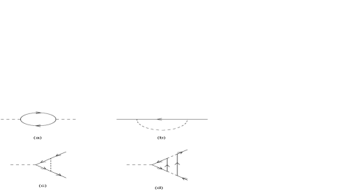
Figure 1: Order $\mathcal{O}(1/N)$ graphs

To the leading order of the large $N$ expansion the quantum action reads

$$\Gamma=\int\mathrm{d}^{d}x\,\sum_{I=0}^{K}\sum_{i=1}^{N_{I}}\overline{\psi}_{i}^{I}\partial\!\!\!/\psi_{i}^{I}+\int{\frac{\mathrm{d}^{d}k}{(2\pi)^{d}}}|\sigma(k)|^{2}\sqrt{k^{2}}D^{-1}(\alpha_{J},r_{J}),$$ (2.9)

This is a Gaussian theory, with a non-local kinetic term for $\sigma$. The couplings are inert and no flow takes place. In this limit, the UV and IR fixed points are indistinguishable, and the constant $D(\alpha_{J},r_{J})$ can be reabsorbed in $\sigma$. It is immediate to check that the zeroth-order expression (2.9) of $\Gamma$ is invariant under the duality transformation (2.5).

The first order of the large $N$ expansion. The RG flow can be inspected computing the $\mathcal{O}(1/N)$ corrections. The relevant graphs are the one-loop fermion self-energy and the one-loop vertex (see Fig. 1) [1]. A two-loop graph ($d$) containing a fermion triangle could in principle contribute to the vertex, but it is zero because of the conservation of chirality.

After resumming the fermion bubbles, the number of relevant graphs becomes finite at each order of the $1/N$ expansion. This means that the $\alpha_{I}$-dependence can be determined exactly, order by order in the $1/N$ expansion. Moreover, this knowledge is sufficient to connect the fixed points, so that it is possible to write $\alpha_{I}$-exact beta functions and correlation functions to any given order of the $1/N$ expansion. The order-$\mathcal{O}(1/N)$ expressions of the beta functions and anomalous dimensions allow us to resum the leading logs (see next section).

The order-$\mathcal{O}(1/N)$ renormalization constants can be written using the results of [1] and read

$$Z_{\psi}^{I} = 1-{\frac{2}{3\pi^{2}N\varepsilon}}\alpha_{I}\mu^{-\varepsilon}D(\alpha_{J},r_{J}),\qquad Z_{\sigma}=1+{\frac{16}{3\pi^{2}N\varepsilon}}\mu^{-\varepsilon}D(\alpha_{J},r_{J}),$$ (2.10)

$$Z_{I} = 1+{\frac{16}{3\pi^{2}N\varepsilon}}(\alpha_{I}-1)\mu^{-\varepsilon}D(\alpha_{J},r_{J}).$$

These expressions are correct also for $I=0$. The factors $D(\alpha_{J},r_{J})$ are brought by the $\sigma$-propagators. The factor $\mu^{-\varepsilon}$ should be understood as a short form for $\lambda_{\mathrm{B}}^{2}N\mu^{-\varepsilon}/4$, so that, using (2.4),

$$\lim_{\varepsilon\rightarrow 0}\frac{\mathrm{d}}{\mathrm{d}\ln\mu}\left[\frac{1}{\varepsilon}\left(\frac{\lambda_{\mathrm{B}}^{2}N\mu^{-\varepsilon}}{4}\right)^{m}\right]=-m.$$

We immediately derive anomalous dimensions and beta functions:

$$\gamma_{\psi}^{I} = {\frac{1}{2}}{\frac{\mathrm{d}\ln Z_{\psi}^{I}}{\mathrm{d}\ln\mu}}={\frac{1}{3\pi^{2}N}}\alpha_{I}D(\alpha_{J},r_{J}),\qquad\gamma_{\sigma}={\frac{1}{2}}{\frac{\mathrm{d}\ln Z_{\sigma}}{\mathrm{d}\ln\mu}}=-{\frac{8}{3\pi^{2}N}}D(\alpha_{J},r_{J}),$$

$$\beta_{I}(\alpha) = -\alpha_{I}{\frac{\mathrm{d}\ln Z_{I}}{\mathrm{d}\ln\mu}}={\frac{16}{3\pi^{2}N}}{\alpha_{I}(\alpha_{I}-1)}D(\alpha_{J},r_{J}).$$ (2.11)

The duality (2.5) can be checked explicitly in these formulas. The only non-straightforward step in this check is the trasformation of $\gamma_{\sigma}$:

$$\gamma_{\sigma}\rightarrow\gamma_{\sigma}-{\frac{1}{2\alpha_{\bar{I}}}}\beta_{\bar{I}}\equiv\widetilde{\gamma}_{\sigma}^{\bar{I}},$$ (2.12)

which is implied by $\sigma\rightarrow\sigma\sqrt{r_{\bar{I}}}\lambda_{\bar{I}}/\lambda_{0}$. We are going to check duality also in the exact expressions of the correlation functions of the next section. From the duality relation (2.12) we recover the formula for the beta function derived in [1],

$$\beta_{\bar{I}}=2\alpha_{\bar{I}}\left(\gamma_{\sigma}-\widetilde{\gamma}_{\sigma}^{\bar{I}}\right),$$

which is exact.

Solution of the RG equations. The RG flow can be integrated immediately in the space of couplings. We have

$${\frac{\mathrm{d}\alpha_{I}}{\alpha_{I}(\alpha_{I}-1)}}={\frac{\mathrm{d}\alpha_{J}}{\alpha_{J}(\alpha_{J}-1)}}$$ (2.13)

for every $I$ and $J$. The solution of (2.13) is

$${\frac{1}{\alpha_{I}}}-1=C_{IJ}\left({\frac{1}{\alpha_{J}}}-1\right),$$ (2.14)

with no summation over $J$. The matrix $C_{IJ}$ is a matrix of arbitrary constants. Restricting to $0\leq\alpha_{I}\leq 1$, self-consistency of (2.14) demands that $C_{IJ}$ satisfies

$$C_{IJ}\geq 0,\qquad C_{IJ}C_{JL}=C_{IL},\qquad C_{IJ}={\frac{1}{C_{JI}}},$$

where, again, no summation on $J$ is understood. The most general solution to these constraints is determined by the constants $C_{I}\equiv C_{1I}$ with $C_{IJ}=C_{J}/C_{I}$. We can write

$$\alpha_{I}={\frac{C_{I}\alpha}{1+(C_{I}-1)\alpha}},$$ (2.15)

where $\alpha\equiv\alpha_{1}$. The choices $C_{I}=0,1,\infty$ for some $I$s correspond to freeze some sets of fermions or glue them to other sets of fermions.

The dependence on the energy is obtained solving the RG equation

$$\beta(\alpha)={\frac{16}{3\pi^{2}N}}{\frac{\alpha(\alpha-1)}{1+r_{1}\alpha+\sum_{J=2}^{K}C_{J}r_{J}\alpha/\left(1+(C_{J}-1)\alpha\right)}}=-{\frac{\mathrm{d}\alpha}{\mathrm{d}t}},$$

where $t=\ln|x|\mu$ and $|x|$ is the overall scale of the correlation function. This equation can always be solved implicitly in the form $t=t(\alpha)$. In general, the function $t(\alpha)$ can be inverted only numerically, but in the simplest case ($K=1$, $r_{1}=1$) it can be inverted also explicitly. The solution is then

$$\alpha(1/|x|)=1+u-\sqrt{u(u+2)},\qquad u={\frac{(1-\alpha(\mu))^{2}}{2\alpha(\mu)}}\left(|x|\mu\right)^{-16/(3\pi^{2}N)}.$$

We have $\alpha(1/|x|)\rightarrow 0$ for $|x|\rightarrow 0$ (ultraviolet) and $\alpha(1/|x|)\rightarrow 1$ for $|x|\rightarrow\infty$ (infrared). For $K=1$ and $r_{1}=r$ generic we have

$$\left(|x|\mu\right)^{-16/(3\pi^{2}N)}={\frac{\alpha(\mu)}{\alpha(1/|x|)}}\left({\frac{1-\alpha(1/|x|)}{1-\alpha(\mu)}}\right)^{r+1}.$$

3 Correlation functions in fermion models

In this section I show how the integration of the RG flow allows us to write all correlation functions exactly in $\alpha$ to any given order in $1/N$. Here it is understood that $\ln\mu\sim N$, because the powers of $(\ln\mu)/N$ are resummed. In particular, to write the correlation functions at the leading-log level, it is sufficient to know the beta function and renormalization constants to the order $1/N$. For concreteness, I choose $K=1$ and $r=1$. This model has two sets of fermions, $\psi^{0}$ and $\psi^{1}$, and one coupling constant $\alpha$.

The $\sigma$ two-point function. Using the Callan-Symanzik equations we know that the $\sigma$ two-point function has the form

$$\langle\sigma(x)\,\sigma(0)\rangle=Z_{\sigma}^{-1}(\alpha(1/|x|),\alpha(\mu)){\frac{A(\alpha(1/|x|))}{2\pi^{2}|x|^{2}}}.$$

At the leading-log level, we need $\gamma_{\sigma}$ to $\mathcal{O}(1/N)$, given by (2.11), and $A$ to $\mathcal{O}(1)$, which is just $1/(1+\alpha)$, from (2.8). We find

$$Z_{\sigma}(\alpha(1/|x|),\alpha(\mu))=\exp\left(-2\int_{\ln\mu}^{-\ln|x|}\gamma_{\sigma}(\mu^{\prime})\ \mathrm{d}\ln\mu^{\prime}\right)={\frac{1-\alpha(1/|x|)}{\alpha(1/|x|)}}{\frac{\alpha(\mu)}{1-\alpha(\mu)}}$$

and therefore

$$\langle\sigma(x)\,\sigma(0)\rangle={\frac{1}{2\pi^{2}|x|^{2}}}{\frac{\alpha(1/|x|)}{1-\alpha^{2}(1/|x|)}}{\frac{1-\alpha(\mu)}{\alpha(\mu)}}={\frac{1}{4\pi^{2}|x|^{2}}}{\frac{1}{\sqrt{u(u+2)}}}{\frac{1-\alpha(\mu)}{\alpha(\mu)}}.$$ (3.1)

It is amusing to check the invariance of this correlation function under the duality transformation (2.5). In doing this, remember that two $\sigma$s get a factor $\alpha(\mu)$ in the transformation.

The exact formula (3.1) exhibits the dependence on the reference scale $\mu$, which survives at both critical points and is different in the UV and IR limits. The anomalous dimension varies from $1-8/(3\pi^{2}N)$ in the ultraviolet, to $1-4/(3\pi^{2}N)$ in the infrared, as expected. The UV and IR behaviors are

$$\langle\sigma(x)\,\sigma(0)\rangle\sim{\frac{1}{2\pi^{2}|x|^{2(1-8/(3\pi^{2}N))}}}{\frac{\mu^{16/(3\pi^{2}N)}}{1-\alpha(\mu)}}\text{\qquad and \qquad}\sim{\frac{1}{4\pi^{2}|x|^{2(1-4/(3\pi^{2}N))}}}{\frac{\mu^{8/(3\pi^{2}N)}}{\sqrt{\alpha(\mu)}}},$$

respectively.

The fermion two-point functions. With the same procedure, the fermion two-point functions are found to be

$$\langle\overline{\psi}^{0}(x)\,\psi^{0}(0)\rangle = {\frac{x\!\!\!/}{4\pi|x|^{3}}}\left[{\frac{1-\alpha(1/|x|)}{\alpha(1/|x|)}}{\frac{\alpha(\mu)}{1-\alpha(\mu)}}\right]^{1/8},$$

$$\langle\overline{\psi}^{1}(x)\,\psi^{1}(0)\rangle = {\frac{x\!\!\!/}{4\pi|x|^{3}}}\left[{\frac{1-\alpha(1/|x|)}{1-\alpha(\mu)}}\right]^{1/8}.$$

There formulas are interchanged by the duality transformation (2.5) (observe that under duality $\alpha(1/|x|)\rightarrow 1/\alpha(1/|x|)$ and $\alpha(\mu)\rightarrow 1/\alpha(\mu)$).

The $\sigma^{2}$ two-point function. As a further example, we study the two-point function of the composite operator $\sigma^{2}$. This operator has dimension 2, but to the order $1/N$ it does not mix with the fermion bilinears $\overline{\psi}^{0}\psi^{0}$ and $\overline{\psi}^{1}\psi^{1}$ (it is sufficient to consider only one such bilinear, since the $\sigma$ field equation relates the two to each other). The calculation of the order-$\mathcal{O}(1/N)$ anomalous dimension of $\sigma^{2}$ requires the evaluation of the divergent parts of two two-loop diagrams with a fermion loop (see Fig. 2). Since both the fermions with $I=0,1$ circulate in the loops, the result is multiplied by $1+\alpha^{2}$. Since there are two $\sigma$-propagators in these diagrams, the result has also a factor $1/(1+\alpha)^{2}$ . We obtain, taking into account of the combinatorial factor and the number of ways in which the fermions can circulate in the loop,

$$Z_{\sigma^{2}}^{-1}Z_{\sigma}=1+{\frac{4}{N\pi^{2}\varepsilon}}\mu^{-2\varepsilon}{\frac{1+\alpha^{2}}{(1+\alpha)^{2}}}$$

and therefore

$$\gamma_{\sigma^{2}}={\frac{8}{3N\pi^{2}}}{\frac{1-2\alpha+3\alpha^{2}}{(1+\alpha)^{2}}}.$$

Figure 2: Renormalization of the operator $\sigma^{2}$

Integrating the RG equations we find

$$\langle\sigma^{2}(x)\,\sigma^{2}(0)\rangle=Z_{\sigma^{2}}^{-2}(\alpha(1/|x|),\alpha(\mu)){\frac{A_{2}(\alpha(1/|x|))}{8\pi^{4}|x|^{4}}}={\frac{\sqrt{u(u+2)}}{4\pi^{4}|x|^{4}}}{\frac{\alpha(\mu)}{(1-\alpha^{2}(\mu))(1+\alpha(\mu))^{2}}}.$$

The function $A_{2}(\alpha)$ can be read from the order-$\mathcal{O}(1)$ expression of the correlation function, which is the $\sigma$-bubble. We have $A_{2}(\alpha)=1/(1+\alpha)^{2}$.

Again, the correlation function transforms correctly under the duality (2.5).

In the ultraviolet and infrared limits we have

$${\frac{1}{8\pi^{4}|x|^{2(2+8/(3\pi^{2}N))}}}{\frac{\mu^{-16/(3\pi^{2}N)}(1-\alpha(\mu))}{(1+\alpha(\mu))^{3}}\qquad}\text{and\qquad}{\frac{1}{4\pi^{4}|x|^{2(2+4/(3\pi^{2}N))}}}{\frac{\mu^{-8/(3\pi^{2}N)}\sqrt{\alpha(\mu)}}{(1+\alpha(\mu))^{3}},}$$

respectively.

In more generality, the anomalous dimension of the operator $\sigma^{2}$ is

$$\gamma_{\sigma^{2}}={\frac{8}{3\pi^{2}N}}D^{2}(\alpha_{J},r_{J})\left(1+\sum_{J=1}^{K}\alpha_{J}r_{J}(3\alpha_{J}-2)\right)$$

and its transformation under the $\bar{I}$th duality reads $\gamma_{\sigma^{2}}\rightarrow\gamma_{\sigma^{2}}-\beta_{\bar{I}}{/}\alpha_{\bar{I}}.$

Other correlation functions. The integration of the RG flow solves the $\alpha$-dependence and allows us to write the correlation functions exactly in $\alpha$ to any given order in $1/N$. In this expansion, if $s$ denotes the overall scale of the correlation function, $\ln s\mu$ is considered of order $N$ and the powers of $(\ln s\mu)/N$ are resummed. In the previous paragraph I have considered two-point functions explicitly, but the procedure is general.

Let us consider the three-point function

$$\langle\sigma^{2}(x)\,\sigma^{2}(y)\,\sigma^{2}(0)\rangle\equiv G(|x|,|y|,|x-y|).$$

This correlation function can be more conveniently expressed in terms of the variables

$$s=|x|+|y|+|x-y|,\quad\nu_{1}={\frac{|x|}{|y|}}+{\frac{|y|}{|x|}},\quad\nu_{2}={\frac{(x-y)^{2}}{|x||y|}}.$$

The variables $\nu_{1,2}$ are scale-independent and $s$ is the overall scale. We can write

$$G(s,\nu_{1},\nu_{2},\alpha(\mu),N)={\frac{1}{s^{3}}}\sum_{k}{\frac{(\ln s\mu)^{k}}{N^{k}}}f_{k}(\nu_{1},\nu_{2},\alpha(\mu),N).$$

For the leading-log approximation it is sufficient to know the functions $f_{k}$ to the leading order. The Callan-Symanzik equations give

$$G(s,\nu_{1},\nu_{2},\alpha(\mu),N)={\frac{1}{s^{3}}}Z_{\sigma^{2}}^{-3}(\alpha(1/s),\alpha(\mu))G_{\mathrm{red}}(\nu_{1},\nu_{2},\alpha(1/s),N)$$

and it is sufficient to compute $G_{\mathrm{red}}(\nu_{1},\nu_{2},\alpha(1/s),N)$ to the leading order in $1/N$. We have

$$\langle\sigma^{2}(x)\,\sigma^{2}(y)\,\sigma^{2}(0)\rangle={\frac{1}{\pi^{6}|x||y||x-y|}}\left(4u(s)(u(s)+2)\right)^{3/4}\left({\frac{\alpha(\mu)}{(1-\alpha^{2}(\mu))(1+\alpha(\mu))^{2}}}\right)^{3/2},$$ (3.2)

where $u(s)=(s\mu)^{-16/(3\pi^{2}N)}(1-\alpha(\mu))^{2}/(2\alpha(\mu))$. If we choose a different definition of the variable $s$, formula (3.2) is unaffected at the level of leading logs.

4 The $r=0$ limit

A particularly simple limit is the case in which the $r_{I}$s are zero. Setting $r_{I}=0$, $I=1,\ldots K$, after expanding in $1/N$ is not equivalent to kill the fermions with $I=1,\ldots K$. The large $N$ and $r_{I}\rightarrow 0$ limits conflict and leave a non-trivial remnant. When $r_{I}=0$, however, duality is not manifest. We can see this immediately from the expression of the beta function:

$$\beta_{I}(\alpha)={\frac{16}{3\pi^{2}N}}{\alpha_{I}(\alpha_{I}-1)}.$$

The RG flow interpolates between $\alpha=0$ and $\alpha=1$, but cannot reach the fixed point at $\alpha=\infty$. To reach $\alpha=\infty$ we have to perform a dual limit in which some or all of the $r_{I}$s tend to infinity. The solution reads

$$\alpha_{I}(1/|x|)={\frac{\alpha(\mu)}{\alpha(\mu)+(1-\alpha(\mu))C_{I}^{-1}(|x|\mu)^{-16/(3\pi^{2}N)}}},$$

where $\alpha\equiv\alpha_{1}$ and $C_{1}=1$. Formula (2.15) still holds. The anomalous dimensions are

$$\gamma_{\psi}^{I}={\frac{1}{3\pi^{2}N}}\alpha_{I},\qquad\gamma_{\sigma}=-{\frac{8}{3\pi^{2}N}},\qquad\gamma_{\sigma^{2}}={\frac{8}{3\pi^{2}N}}.$$

$\gamma_{\sigma}$ and $\gamma_{\sigma^{2}}$ do not depend on the energy. The other results can be generalized straightforwardly to this case.

5 Models with two-component spinors and new fixed points

Let us now consider a variant of the model (2.1) in which the spinors have two complex components instead of four.

We have no chiral invariance (2.2) and the transformation (2.3) does not apply. For this reason, the signs of the couplings $g_{I}$ cannot be assumed to be positive. The P and T transformations are modified as follows:

$$P_{1} : \qquad x_{1}\rightarrow-x_{1},\qquad x_{2,3}\rightarrow x_{2,3},\qquad\psi_{i}^{I}\rightarrow\gamma_{1}\psi_{i}^{I},\qquad\sigma\rightarrow-\sigma\ ;$$ (5.1)

$$T : \qquad x_{3}\rightarrow-x_{3},\qquad x_{1,2}\rightarrow x_{1,2},\qquad\psi_{i}^{I}\rightarrow\gamma_{3}\psi_{i}^{I},\qquad\overline{\psi}_{i}^{I}\rightarrow\overline{\psi}_{i}^{I}\gamma_{3},\qquad\sigma\rightarrow-\sigma.$$

The theory is still invariant under the duality (2.5) and we can assume that $-1\leq g_{I}\leq 1$.

To avoid the problem of extending to $d$ dimensions a Dirac algebra in which the trace of an odd number of gamma matrices does not vanish, it is better to keep $d=3$ and regularize the theory modifying the $\psi$- and $\sigma$-quadratic terms with a cut-off as follows:

$$\overline{\psi}\partial\!\!\!/\left(1-{\frac{\Box}{\Lambda^{2}}}\right)\psi,\qquad\mathrm{and}\qquad{\frac{1}{2}}|\sigma(k)|^{2}\sqrt{k^{2}}\left(1+{\frac{k^{2}}{\Lambda^{2}}}\right)D(g_{I}^{2},r_{I}).$$

This regularization framework manifestly preserves the P and T symmetries (5.1) (a Pauli-Villars framework does not) and ensures that no $\sigma^{3}$ term is generated by renormalization. The graphs with an odd number of $\sigma$ external legs are finite, but need not vanish.

The wave-function renormalization constants and beta functions are the same as in (2.10) and (2.11) with $N\rightarrow N/2$. In particular, the $g_{I}$ beta functions read

$$\beta_{I}(g)=-\frac{g_{I}}{2}{\frac{\mathrm{d}\ln Z_{I}}{\mathrm{d}\ln\mu}}={\frac{8}{3\pi^{2}N}g}{{}_{I}(g_{I}^{2}-1)}D(g_{J}^{2},r_{J}).$$ (5.2)

We see that the fixed points of this model are $\left\{g_{I}\right\}$= any string made of $1,0,-1$. These fixed points have the form

$$\Psi_{N_{f}}\otimes F_{2}\Sigma_{N_{\sigma},N_{\sigma}^{\prime}},$$

where $N_{f}$ is the number of decoupled fermions (coupling $g_{I}=0$), $N_{\sigma}$ is the number of fermions interacting with $\sigma$ with coupling $g_{I}=1$ and $N_{\sigma}^{\prime}$ is the number of fermions interacting with $\sigma$ with coupling $g_{I}=-1$. The conformal field theories $F_{2}\Sigma_{N_{\sigma},N_{\sigma}^{\prime}}$ are defined by the lagrangian

$$\mathcal{L}=\sum_{i=1}^{N_{\sigma}}\overline{\psi}_{i}(\partial\!\!\!/+\lambda\sigma)\psi_{i}+\sum_{i=j}^{N_{\sigma}^{\prime}}\overline{\chi}_{j}(\partial\!\!\!/-\lambda\sigma)\chi_{j}.$$ (5.3)

and have symmetry $O(2N_{\sigma})\otimes O(2N_{\sigma}^{\prime})$. The subscript 2 in $F_{2}\Sigma_{N_{\sigma},N_{\sigma}^{\prime}}$ means that the spinors are two-component. In general ($r\neq 1$), the conformality of (5.3) does not seem to be implied by more general principles than the vanishing of the beta function (5.2) at $g=-1$. The symmetries of the model allow us to construct a local, dimension-3 operator $O$ that does not vanish using the field equations (for example $\sigma\overline{\psi}\psi$) and could appear in the trace anomaly, $\Theta=\beta O$. Instead, at $r=1$ the two-component spinors $\psi$ and $\chi$ can be grouped into a four-component spinor and we have $F_{2}\Sigma_{N,N}=F_{4}\Sigma_{N}$, whose conformality follows from the general arguments of [1].

The $F_{2}\Sigma_{N_{\sigma},N_{\sigma}^{\prime}}$ theories have also a duality

$$\psi\leftrightarrow\chi,\qquad\sigma\rightarrow-\sigma\sqrt{r},\qquad\lambda\rightarrow\lambda/\sqrt{r},\qquad r\rightarrow 1/r,\qquad N_{\sigma}\leftrightarrow N_{\sigma}^{\prime},$$

where $r=N_{\sigma}^{\prime}/N_{\sigma}$ and $\lambda^{2}N_{\sigma}=8$.

The order $\mathcal{O}(1/N)$ anomalous dimensions $\gamma_{\psi}^{I}$ and $\gamma_{\sigma}$ of the theories $F_{2}\Sigma_{N,N^{\prime}}$ coincide with those of the theories $F_{2}\Sigma_{N+N^{\prime}}$ (and $F_{4}\Sigma_{N/2,N^{\prime}/2}$, $F_{4}\Sigma_{(N+N^{\prime})/2}$), but the symmetry groups differ.

It is straightforward to extend the other results of the previous sections to the flows interpolating between the $F\Sigma_{N,N^{\prime}}$ models.

6 Scalar models

We now consider the scalar models

$$\mathcal{L}={\frac{1}{2}}\sum_{I=0}^{K}\sum_{i=1}^{N_{I}}\left[(\partial_{\mu}\varphi_{i}^{I})^{2}+i\lambda_{I}\sigma(\varphi_{i}^{I})^{2}\right]+V_{6}(\varphi),$$ (6.1)

with symmetry group $\bigotimes_{I=0}^{K}O(N_{I})$, possibly enhanced at the fixed points. The $\lambda_{I}$s are not necessarily positive and $V_{6}(\varphi)$ denotes a potential term of the form $\varphi^{6}$ induced by renormalization.

Scalar $\Sigma_{N}$ conformal field theories. I define the scalar $\Sigma_{N}$ conformal theories by means of the lagrangian

$$\mathcal{L}={\frac{1}{2}}\sum_{i=1}^{N}\left[(\partial_{\mu}\varphi_{i})^{2}+i\lambda_{I}\sigma(\varphi_{i})^{2}\right],$$ (6.2)

which I briefly denote with $S\Sigma_{N}$. This theory coincides with the UV (Wilson-Fischer) fixed point of the $O(N)$ sigma model. In the approach of [1], the $S\Sigma_{N}$ model can be studied per se, with no reference to an RG flow generating it as a critical limit. The construction of the theories $S\Sigma_{N}$ follows the lines of the construction of the fermionic theories $F\Sigma_{N}$ of [1]. A caveat is that renormalization generates a $\varphi^{6}$ term. Due to the $O(N)$ symmetry, this term can only have the form

$$\left(\sum_{i=1}^{N}\varphi_{i}^{2}\right)^{3}$$ (6.3)

and so can be reabsorbed with an (imaginary) translation of the field $\sigma$. This is equivalent to say that (6.3) is “trivial” because proportional to the $\sigma$ field equation. The $\sigma$ field equation formally sets the composite operator $\varphi^{2}$ to zero, but does not trivialize the theory. More details on the use of the $\sigma$ field equation can be found in the appendix.

The theory is classically conformal and we choose the classically conformal subtraction scheme, in which the renormalized $\varphi^{2}$- and $\varphi^{4}$-terms are set to zero by default.

The $\sigma$-propagator is generated by the one-loop scalar bubble, which is proportional to $(k^{2})^{d/2-2}$. If unmodified, a $\sigma$-propagator $\sim(k^{2})^{2-d/2}$ generates $\Gamma[0]$s at the subleading orders. It is therefore necessary to add an evanescent, RG-invariant, non-local term to the lagrangian and convert the $\sigma$-propagator to $\sqrt{k^{2}}$. This means, in particular, that the field $\sigma$ has dimension $\left(d+1\right)/2$ and $\lambda_{\mathrm{B}}=\lambda\mu^{\varepsilon/2}$. The $O(1/N)$ diagrams are the same as in Fig. 1. The diagram ($d$) does not vanish identically, but is finite. Finally, the $O(1/N)$ results for $\gamma_{\varphi}$ and $\gamma_{\sigma}$ are equal to those of the $F\Sigma_{N}$ models (2.7), with the replacement $N\rightarrow N/4$.

The running $S\Sigma_{N}$ models. Let us now consider the theories (6.1). We can still use the classically conformal substraction scheme, and therefore assume that the terms of the form $\varphi^{2}$ and $\varphi^{4}$ are subtracted away by default. However, nothing forbids the generation of terms of the form $\varphi^{6}$ and this time they cannot be removed with a translation of the field $\sigma$. The reason is that $\sigma$ multiplies

$$\sum_{I=0}^{K}\lambda_{I}(\varphi^{I})^{2},$$

but the $\varphi^{6}$ divergences can be proportional to

$$\left(\sum_{I=0}^{K}\alpha_{I}^{m}(\varphi^{I})^{2}\right)\left(\sum_{I=0}^{K}\alpha_{J}^{n}(\varphi^{J})^{2}\right)\left(\sum_{I=0}^{K}\alpha_{L}^{p}(\varphi^{L})^{2}\right)$$

with $m$, $n$ and $p$ generic. It is therefore necessary to introduce the most general $\varphi^{6}$-vertices in the lagrangian, multiplied by independent couplings.

For simplicity, I focus on a model with two sets of scalar fields, $\varphi_{i}$, $i=1,\ldots N$ and $\chi_{j}$, $j=1,\ldots Nr$, $K=2$. The lagrangian reads

$$\mathcal{L}={\frac{1}{2}}\sum_{i=1}^{N}(\partial_{\mu}\varphi_{i})^{2}+{\frac{1}{2}}\sum_{j=1}^{Nr}(\partial_{\mu}\chi_{j})^{2}+i{\frac{\lambda}{2}}\sigma\left(\sum_{i=1}^{N}\varphi_{i}^{2}+g\sum_{j=1}^{Nr}\chi_{j}^{2}\right)+{\frac{32\lambda_{60}}{N^{2}}}\left(\sum_{i=1}^{N}\varphi_{i}^{2}\right)^{3}+{\frac{32\lambda_{06}}{N^{2}r^{2}}}\left(\sum_{j=1}^{Nr}\chi_{j}^{2}\right)^{3}.$$ (6.4)

The factors in front of the $V_{6}$-vertices are chosen for notational convenience.

The duality transformation is

$$g\rightarrow{\frac{1}{g}},\qquad\varphi\leftrightarrow\chi,\qquad r\rightarrow{\frac{1}{r}},\qquad\lambda_{60}\leftrightarrow\lambda_{06},\qquad\lambda\rightarrow{\frac{\lambda}{\sqrt{r}}},\qquad\sigma\rightarrow\sigma g\sqrt{r}.$$ (6.5)

I have dropped vertices of the form $\varphi^{4}\chi^{2}$ and $\varphi^{2}\chi^{4}$, since they can always be reabsorbed with a $\sigma$-translation while keeping duality manifest. The remaining $V_{6}$-vertices are redundant (one suffices), but cannot be reduced to a single vertex in the full space of parameters using the $\sigma$-field equation. We have to divide the parameter space into two charts, one contaning $g=0$ and the other containing $g=\infty$. In the first chart, the $\varphi^{6}$ vertex is trivial and can be reabsorbed into a $\sigma$-translation. However, the $\chi^{6}$ vertex cannot be reabsorbed into a $\sigma$ translation at the point $g=0$. Therefore, in the first chart we remove the $\varphi^{6}$ vertex setting $\lambda_{60}=0$ and take $\lambda_{06}$ as the unique $V_{6}$-coupling. In the second chart, which contains $g=\infty$, we have a symmetric situation: the $\chi^{6}$ vertex can be reabsorbed away, but the $\varphi^{6}$ vertex cannot, so we set $\lambda_{06}=0$ and the true coupling is $\lambda_{60}$.

In each chart we have an appropriate specialization of the duality transformation (6.5). For example, when we apply duality in the first chart, we transform the potential $\lambda_{60}\varphi^{6}/N^{2}$ into $\widetilde{\lambda}_{60}\chi^{6}/(N^{2}r^{2})$. Then, we can use the $\sigma$-field equation $\chi^{2}=-\varphi^{2}/g$ and rewrite the potential as $-\widetilde{\lambda}_{60}\varphi^{6}/(r^{2}g^{3}N^{2})$. To recover the initial potential we define $\widetilde{\lambda}_{60}=-r^{2}g^{3}\lambda_{60}$, so that duality in the first chart reads

$$g\rightarrow{\frac{1}{g}},\qquad\varphi\leftrightarrow\chi,\qquad r\rightarrow{\frac{1}{r}},\qquad\lambda_{60}\rightarrow-r^{2}g^{3}\lambda_{60},\qquad\lambda\rightarrow{\frac{\lambda}{\sqrt{r}}},\qquad\sigma\rightarrow\sigma g\sqrt{r}.$$ (6.6)

A symmetric argument allows us to specialize the duality transformation to the second chart. Invariance under duality is a powerful tool to check the calculations.

The leading and subleading order in the $\sigma$-sector. The effective $\sigma$-propagator is obtained resumming the scalar bubbles and reads

$$\langle\sigma(k)\,\sigma(-k)\rangle=\sqrt{k^{2}}D(\alpha_{J},r_{J}).$$

To the order $\mathcal{O}(1/N)$, the $\varphi^{6}$ and $\chi^{6}$ vertices have no effect on the renormalization of the scalar kinetic terms and the $\sigma$-scalar-scalar vertices. This can be proved observing that the relevant graphs are in one-to-one correspondence with the graphs of Fig. 4 contaning four scalar external legs exiting from the same six-leg vertex. I call these graphs $\mathcal{G}_{4,2}$ for clarity.

$i$) The graphs contributing to the renormalization of the scalar propagator are obtained from $\mathcal{G}_{4,2}$ suppressing the four external scalar legs exiting from the same six-leg vertex. We obtain the graph (b) of Fig.1 plus tadpoles, finite graphs and a graph with a scalar bubble (from the third of Fig. 4). This graph should not be counted, since the scalar bubbles are resummed into the $\sigma$-propagator.

$ii$) The graphs contributing to the renormalization of the $\sigma$-scalar-scalar vertices are obtained from $\mathcal{G}_{4,2}$ replacing the four external scalar legs exiting from the same six-leg vertex with one external $\sigma$ leg. We obtain the graphs (c) and (d) of Fig. 1 plus tadpoles and finite graphs.

In summary, the order $\mathcal{O}(1/N)$ anomalous dimensions and beta functions are exactly the same as in (2.11), with $N\rightarrow N/4$. In particular, we have

$$\beta_{g}={\frac{32}{3N\pi^{2}}}{\frac{g(g^{2}-1)}{1+rg^{2}}}.$$

The zeroes are at $g=-\infty,-1,0,1,\infty$.

The $\varphi^{6}$-terms. Now we study the induction of a $V_{6}$-coupling by renormalization. The order $\mathcal{O}(1/N)$ beta function of the $\varphi^{6}$-coupling reads in the first chart

$$\beta_{60} = {\frac{32}{3N\pi^{2}(1+rg^{2})^{3}}}\left[-(1-g)^{3}+3\lambda_{60}\left(1+3g^{2}+2rg^{2}+6rg^{3}+4r^{2}g^{4}\right)\right.$$ (6.7)

$$\left.\qquad\qquad\qquad\qquad\qquad\qquad-27\lambda_{60}^{2}rg^{3}(1-r^{2}g^{3})-27\lambda_{60}^{3}r^{3}g^{6}\right].$$

Graphs and details on the calculation are given in the appendix. This formula transforms correctly under the duality (6.6), i.e.

$$\beta_{60}\rightarrow-r^{2}g^{3}\beta_{60}-3\lambda_{60}r^{2}g^{2}\beta_{g}.$$ (6.8)

In the second chart we have

$$\beta_{06} = {\frac{32}{3Nr\pi^{2}(1+rg^{2})^{3}}}\left[r^{3}g^{3}(1-g)^{3}+3\lambda_{06}rg^{2}\left(4+6rg+2rg^{2}+3r^{2}g^{2}+r^{2}g^{4}\right)\right.$$

$$\left.\qquad\qquad\qquad\qquad\qquad\qquad+27\lambda_{06}^{2}(1-r^{2}g^{3})-27\lambda_{06}^{3}\right].$$

Fixed points. At $g=\infty$ and $g=0$ we work in the first and second chart, respectively, and find the beta function of ref.s [7], namely

$$\beta_{60}={\frac{288}{N\pi^{2}}}\lambda_{60}^{2}(1-\lambda_{60}),\qquad\beta_{06}={\frac{288}{Nr\pi^{2}}}\lambda_{06}^{2}(1-\lambda_{06}).$$ (6.9)

The solutions of $\beta_{60}=0$ are $\lambda_{60}^{*}=0$ and $\lambda_{60}^{*}=1$. At $\lambda_{60}^{*}=0$ the fixed point is the direct product of an $S\Sigma_{Nr}$ model and $N$ free scalars. At $\lambda_{60}=1$ the fixed point is the direct product of $S\Sigma_{Nr}$ and the interacting $\varphi_{3}^{6}$ fixed point. In both cases, the flavor symmetry group is $O(N)\otimes O(Nr)$. The negative values of $\lambda_{60}$ and $\lambda_{60}$ are unphysical at $g=\infty$ and $g=0$, becuse the potential is unbounded from below.

For $g=1$ we have

$$\beta_{60}={\frac{32\lambda_{60}}{N\pi^{2}(1+r)^{3}}}\left[4(1+r)^{2}-9\lambda_{60}r(1-r^{2})-9\lambda_{60}^{2}r^{3}\right].$$

The solutions of $\beta_{60}=0$ are $\lambda_{60}^{*}=0$ and the two interacting fixed points

$$\lambda_{60}^{*}={\frac{1+r}{6r^{2}}}\left(3(r-1)\pm\sqrt{9-2r+9r^{2}}\right),$$

which are interchanged by duality. At $\lambda_{60}=0$ the fixed point is an $S\Sigma_{N(1+r)}$ model.

For $g=-1$ we have

$$\beta_{60}={\frac{32}{3N\pi^{2}(1+r)^{3}}}\left[-8+12\lambda_{60}(1-r+r^{2})+27\lambda_{60}^{2}r(1+r^{2})-27\lambda_{60}^{3}r^{3}\right].$$

The equation $\beta_{60}=0$ has three real solutions, two positive and one negative. For $r\rightarrow\infty$ the largest positive solution tends to $1$ from above, the second positive solution $\bar{\lambda}_{60}$ tends to $0^{+}$ and the negative solution tends to $0^{-}$.

The fixed point $(g,\lambda_{60})=(0,1)$ is UV unstable, while the fixed points $(1,0)$ and $(-1,\bar{\lambda}_{60})$ are IR stable. The other fixed points are partially stable and partially unstable.

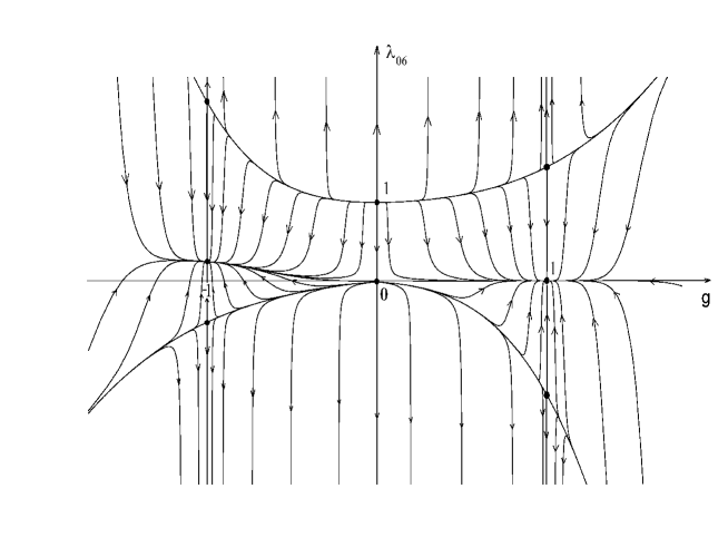
Figure 3: The fixed points and RG flows of the scalar models

The RG flows are plotted in Fig. 3. Since at $g=0$ the negative values of $\lambda_{60}$ are unphysical, we can argue that the unphysical region is the region below the line connecting the three fixed points with $\lambda_{60}^{*}\leq 0$.

A particularly simple case is the limit $r\rightarrow\infty$, where $\beta_{60}$ is independent of $g$ and coincides with (6.9). Here the RG flows of $g$ and $\lambda_{60}$ separate.

7 Conclusions

In the realm of high-energy physics, classically conformal theories play a special role. Taking inspiration from massless QCD, where hadrons and glueballs acquire masses dynamically, it is tempting to think that the ultimate theory of the universe contains no dimensionful parameter of classical origin, the classically conformal subtraction scheme should be universally used and the dynamical generation of a scale $\mu$ by dimensional transmutation originates all scales and dimensionful parameters of nature, including the Newton constant.

Another context in which the specialness of classically conformal theories is singled out, at least in even dimensions, is the irreversibility of the RG flow. It would be interesting to know if the RG flow is irreversible also in odd dimensions. The flows of this paper are used for this investigation in ref. [11].

It is useful to have a large class of classically conformal models to test ideas around the issues just mentioned and the strongly-coupled limit of quantum field theory. I believe that the models studied in this paper can help us answering various unsolved problems and have a number of potential applications, maybe also in condensed-matter physics.

I have explored two classes of theories, describing sets of fermions and scalar fields interacting by means of a $\sigma$-field, with a variety of fixed points, known and new. Typically, both end points of the flows are interacting conformal field theories. The remarkable properties of these theories are that $i$) at each order of the $1/N$ expansion the RG flows can be integrated for arbitrary values of the running couplings; $ii$) “exact” beta functions, anomalous dimensions and correlation functions interpolating between the UV and IR conformal limits can be written; $iii$) the models have manifest $g\rightarrow 1/g$ dualities at each order of the $1/N$ expansion. Duality puts severe constraints on the formulas and is a powerful tool to check the calculations. In special limits ($r\rightarrow 0$ in the fermionic models, $r\rightarrow\infty$ in the scalar models) the integration of the flow equations further simplifies, yet the flow remains non-trivial.

Appendix: diagrammatics and duality in the scalar models

The graphs contributing to the renormalization of $\varphi^{6}$ to the order $\mathcal{O}(1/N)$ are shown in Fig. 4. Some diagrams have obvious counterparts with two, four and six external $\chi$-legs. The divergent terms proportional to $\varphi^{2}\chi^{4}$, $\varphi^{4}\chi^{2}$ and $\chi^{6}$ are converted to $\varphi^{6}$ using the $\sigma$-field equation $\varphi^{2}+g\chi^{2}=0$. (For subtleties in the use of this field equation see below.) Several diagrams are finite, but have been drawn for completeness.

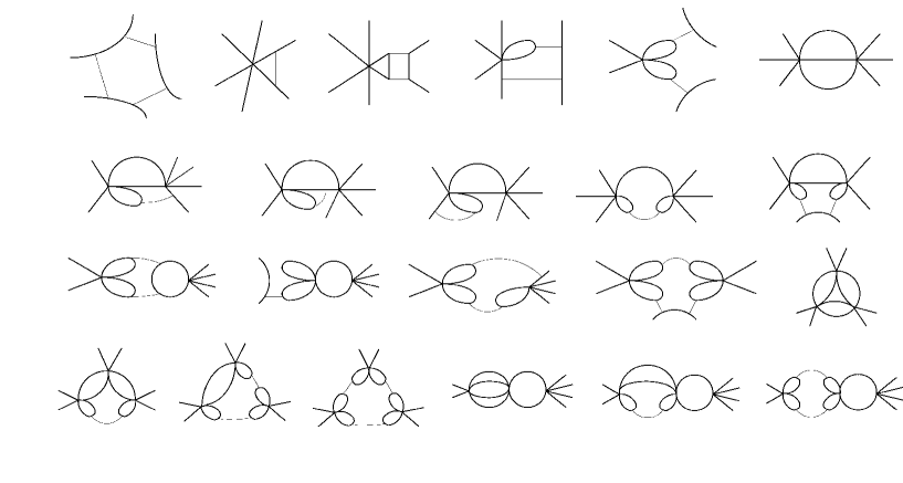
Figure 4: Renormalization of $\varphi^{6}$ in the scalar models

The beta function (6.7) is invariant under the duality symmetry (6.6) and (6.8). However, the renormalization constant $Z_{60}$ is not. The complete expression of $\lambda_{60}Z_{60}$ is very long and contains terms with the first three powers of $\lambda_{60}$ plus a term independent of $\lambda_{60}$. Here I focus on the terms proportional to $\lambda_{60}^{3}$, for simplicity, which are

$$-{\frac{288\lambda_{60}^{3}}{N\pi^{2}}}\left({\frac{\mu^{-4\varepsilon}}{4\varepsilon}}-{\frac{3\mu^{-5\varepsilon}}{5\varepsilon(1+rg^{2})}}+{\frac{\mu^{-6\varepsilon}}{2\varepsilon(1+rg^{2})^{2}}}-{\frac{\mu^{-7\varepsilon}}{7\varepsilon(1+rg^{2})^{3}}}\right).$$ (7.10)

Expanding $\mu^{-m\varepsilon}/(m\varepsilon)$ as $1/(m\varepsilon)-\ln\mu$ we see that the terms proportional to $\ln\mu$, which contribute to the beta function, transform correctly under duality, while the pole terms, which have no physical significance, do not transform correctly.

These facts are explained as follows. The symmetry of the theory under the duality transformation (6.6) in the first chart understands the use the $\sigma$ field equation. Naively, the $\sigma$ field equation is $\varphi^{2}+g\chi^{2}=0$, but the modified regularization technique of [1] demands to add the non local term

$$\frac{1+rg^{2}}{2}\int{\frac{\mathrm{d}^{d}k}{(2\pi)^{d}}}|\sigma(k)|^{2}{\frac{1}{\sqrt{k^{2}}}}\left(1-{\frac{\lambda_{\mathrm{B}}^{2}N}{16}}\left(k^{2}\right)^{-\varepsilon/2}\right)$$

to the action $S$. The complete $\sigma$ field equation reads, in momentum space,

$$\varphi^{2}(k)+g\chi^{2}(k)={\frac{2i(1+rg^{2})}{\lambda}}{\frac{1}{\sqrt{k^{2}}}}\left(1-{\frac{\lambda_{\mathrm{B}}^{2}N}{16}}\left(k^{2}\right)^{-\varepsilon/2}\right)\sigma(k).$$

The evanescent right-hand side of this formula provides extra vertices which do contribute to the pole terms. However, these corrections are always proportional to

$${\frac{\mu^{-m_{1}\varepsilon}}{m_{1}\varepsilon}}-{\frac{\mu^{-m_{2}\varepsilon}}{m_{2}\varepsilon}}$$ (7.11)

for some $m_{1}$ and $m_{2}$ and so do not affect the $\ln\mu$ terms. This fact can be easily verified in a number of examples. Moreover, the terms proportional to the $\sigma$ field equation $\delta S/\delta\sigma$ cannot be neglected. They give other contributions of the form (7.11), which can be easily computed functionally integrating by parts. Putting these ingredients together, we discover that the mismatch between $Z_{60}$ and its dual is due to the use of the $\sigma$ field equation and the difference between the naive and regularized $\sigma$ field equations. It is not a lengthy work to make a quantitative check for the terms (7.10). The important point is that the mismatch has no physical significance. We can neglect these nuisances if we limit ourselves to check duality within the physical quantities.

Acknowledgements

I am grateful to the Aspen Center for Physics for warm hospitality during the realization of this work and P. Calabrese, P. Parruccini and E. Vicari for discussions on three-dimensional models and critical phenomena.

References

• [1] D. Anselmi, Large-N expansion, conformal field theory and renormalization-group flows in three dimensions, JHEP 0006 (2000) 042 and hep-th/0005261.
• [2] G. Parisi, The theory of nonrenormalizable interactions. I – The large $N$ expansion, Nucl. Phys. B 100 (1975) 368.
• [3] B. Rosenstein, B. Warr and S.H. Park, Dynamical symmetry breaking in four fermi interaction models, Phys. Rept. 205 (1991) 59.
• [4] V.A. Novikov, M.A. Shifman, A.I. Vainshtein and V.I. Zakharov, Exact Gell-Mann-Low function of supersymmetric Yang-Mills theories from instanton calculus, Nucl. Phys. B 229 (1983) 381.
• [5] D. Anselmi, D.Z. Freedman, M.T. Grisaru and A.A. Johansen, Nonperturbative formulas for central functions in supersymmetric gauge theories, Nucl. Phys. B 526 (1998) 543 and hep-th/9708042.
• [6] D. Anselmi, J. Erlich, D.Z. Freedman and A.A. Johansen, Positivity constraints on anomalies in supersymmetric theories, Phys. Rev. D57 (1998) 7570 and hep-th/9711035.
• [7] P.K. Townsend, Consistency of the $1/N$ expansion for three-dimensional $\phi^{6}$ theory, Nucl. Phys. B 118 (1977) 199; R.D. Pisarski, Fixed point structure of $\phi_{3}^{6}$ at large $N$, Phys. Rev. Lett. 48 (1982) 574; T. Appelquist and U. Heinz, Vacuum stability in three-dimensional $O(N)$ theories, Phys. Rev. D 25 (1982) 2620.
• [8] W.A. Bardeen, M. Moshe and M. Bander, Spontaneous breaking of scale invariance and the ultraviolet fixed point in the $O(N)$ symmetric $\phi_{3}^{6}$ theory, Phys. Rev. Lett. 52 (1984) 1188. F. David, D.A. Kessler and H. Neuberger, The Bardeen-Moshe-Bander fixed point and ultraviolet triviality of $\phi^{6}$ in three dimensions, Phys. Rev. Lett. 53 (1984) 2071.
• [9] D. Anselmi, Sum rules for trace anomalies and irreversibility of the renormalization-group flow, V International Conference Renormalization Group 2002, Strba, Slovakia, March 2002, Acta Physica Slovaka and hep-th/0205039.
• [10] D. Anselmi, Anomalies, unitarity and quantum irreversibility, Ann. Phys. (NY) 276 (1999) 361 and hep-th/9903059.
• [11] D. Anselmi, Inequalities for trace anomalies, length of the RG flow, distance between the fixed points and irreversibility, hepth/0210124.