Abstract

For $m^{2}<a^{2}+q^{2}$, with $m$, $a$, and $q$ respectively the source mass, angular momentum per unit mass, and electric charge, the Kerr-Newman (KN) solution of Einstein’s equation reduces to a naked singularity of circular shape, enclosing a disk across which the metric components fail to be smooth. By considering the Hawking and Ellis extended interpretation of the KN spacetime, it is shown that, similarly to the electron-positron system, this solution presents four inequivalent classical states. Making use of Wheeler’s idea of charge without charge, the topological structure of the extended KN spatial section is found to be highly non-trivial, leading thus to the existence of gravitational states with half-integral angular momentum. This property is corroborated by the fact that, under a rotation of the space coordinates, those inequivalent states transform into themselves only after a $4\pi$ rotation. As a consequence, it becomes possible to naturally represent them in a Lorentz spinor basis. The state vector representing the whole KN solution is then constructed, and its evolution is shown to be governed by the Dirac equation. The KN solution can thus be consistently interpreted as a model for the electron-positron system, in which the concepts of mass, charge and spin become connected with the spacetime geometry. Some phenomenological consequences of the model are explored.

1 Introduction

The stationary axially-symmetric Kerr-Newman (KN) solution of Einstein’s equations was found by performing a complex transformation on the tetrad field for the charged Schwarzschild (Reissner–Nordström) solution [1, 2, 3]. For $m^{2}\geq a^{2}+q^{2}$, it represents a black hole with mass $m$, angular momentum per unit mass $a$ and charge $q$ (we use units in which $\hbar=c=1$). In the so called Boyer–Lindquist coordinates $r,\theta,\phi$, the KN solution is given by [4]

$$ds^{2}=dt^{2}-\frac{\rho^{2}}{\Delta}\,dr^{2}-(r^{2}+a^{2})\sin^{2}\theta\,d\phi^{2}-\rho^{2}\,d\theta^{2}-\frac{Rr}{\rho^{2}}\,(dt-a\sin^{2}\theta\,d\phi)^{2},$$ (1)

where $\rho^{2}=r^{2}+a^{2}\cos^{2}\theta$, $\Delta=r^{2}-Rr+a^{2}$ and $R=2m-q^{2}/r$. This metric is invariant under the simultaneous changes $(t,a)\rightarrow(-t,-a)$, $(m,r)\rightarrow(-m,-r)$, and separately under $q\rightarrow-q$. This black hole is believed to be the final stage of a very general stellar collapse, where the star is rotating and its net charge is different from zero.

The structure of the KN solution changes deeply when $m^{2}<a^{2}+q^{2}$. Due to the absence of an horizon, it does not represent a black hole, but a circular naked singularity in spacetime. This solution is of particular interest because it describes a massive charged object with spin, and with a gyromagnetic ratio equal to that of the electron [2]. As a consequence, several attempts to model the electron by the KN solution have been made [5, 6, 7]. In all these models, however, the circular singularity is somehow surrounded by a massive ellipsoidal shell (bubble), so that it is unreachable. In other words, the singularity is considered to be non-physical in the sense that the presence of the massive bubble precludes its formation.

Inspired in the works by Barut [8, 9], who tried to explain the Zitterbewegung that appears in the electron’s Dirac theory, and also in the works by Wheeler [10] about “matter without matter” and “charge without charge”, we will propose here that the KN solution, without any matter surrounding it, can be consistently interpreted as a realistic model for the electron. Our construction will proceed according to the following scheme. First, by applying to the Kerr-Newman case the Hawking and Ellis extended spacetime interpretation of the Kerr solution [4], some properties of the classical KN solution for $m^{2}<a^{2}+q^{2}$ are reviewed. It is found that, similarly to the electron-positron system, the KN solution presents four inequivalent classical states. Then, an analysis of the topological properties of the space section of the extended KN spacetime is made. As already demonstrated in the literature [11], the possible topologies of three-manifolds fall into two classes, those which allow only vector states with integral spin, and those which give rise to vector states having both integral and half-integral spins. In other words, for a certain class of three-manifolds, the angular momentum of an asymptotically flat gravitational field can present half-integral values, revealing in this way the presence of a spinorial structure. As we are going to see, this is exactly the case of the space section of the Hawking and Ellis extended KN solution, when Wheeler’s idea of charge without charge is taken into account. This will also become evident from the fact that each one of the inequivalent KN states is seen to transform into itself only under a $4\pi$ rotation, a typical property of spinor fields. As a consequence of this property, those states can naturally be represented in a Lorentz spinor basis. By introducing such a basis, the vector state representing the whole KN solution in a rest frame is obtained. Then, the general representation of this vector state with a nonvanishing momentum ($\vec{p}\neq 0$) is found, and its evolution is shown to be governed by the Dirac equation. It is important to remark that the Dirac equation will not be obtained in a KN spacetime. Instead, the KN solution itself (for $m^{2}<a^{2}+q^{2}$) will appear as an element of a vector space, which is a solution of the Dirac equation. Furthermore, as is usually done in particle physics, the gravitational field produced by the electron—here represented by the KN solution—will be supposed to be fast enough asymptotically flat, so that the Dirac equation can be written in a Minkowski background spacetime. The above results suggest that the KN solution can be consistently interpreted as a model for the electron. At the final part of the paper, an analysis of some phenomenological consequences of the model is presented, and a discussion of the results obtained is made.

2 The Extended KN Solution

2.1 Basic properties

The KN solution for $m^{2}<a^{2}+q^{2}$ exhibits a true circular singularity of radius $a$, enclosing a disk across which the metric components fail to be smooth. If the center of the circle is placed at the origin of a Cartesian coordinate system, the circular singularity coincides with the $xy$ plane, and the axial symmetry of the solution (around the $z$-axis) becomes explicit. It should be remarked that, when dealing with such solution, the concepts of mass and charge must be carefully used because the presence of the singularity forbids one to apply both physical concepts and laws along points in the border of the disk. The lack of smoothness of the metric components across the enclosed disk can be remedied by considering the extended spacetime interpretation of Hawking and Ellis [4], although the circular singularity cannot be removed by this process. The basic idea of this extension is to consider that our spacetime is joined to another one by the singular disk. In other words, the disk surface (with the upper points considered different from the lower ones) is interpreted as a shared border between our spacetime, denoted by M, and another similar one, denoted by M’. According to this construction, the KN metric components are no longer singular across the disk, making it possible to smoothly join the two spacetimes, giving rise to a single $4$-dimensional spacetime ${\mathcal{M}}$.

In what follows, we will assume the spacetime extension of Hawking and Ellis. This means that the space sections of the spaces M and M’ are joined through the disks enclosed by the singularity. This linking can be seen as solid cylinders going from one 3-manifold to the other (see Fig. 1). The main consequences of this interpretation are:

• We can associate the electric charge of the KN solution on each $3$-manifold with the net flux of a topologically trapped electric field, which goes from one space to the other, as proposed by Wheeler [10]. Although the electric field lines seem to end at the singular ring (seen from either M or M’), the equality of the electric charge on both sides of $\mathcal{M}$ tells us that no electric field lines can “disappear” when going from M to M’, or vice-versa. Then, in analogy with the geometry of the wormhole solution, there must exist a continuous path for each electric field line going from one space to the other. Furthermore, the equality of magnetic moment on both sides of $\mathcal{M}$ implies that the magnetic field lines must also be continuous when passing through the disk enclosed by the singularity.

• We can associate the mass of the solution with the degree of non-flatness of the KN solution. Actually, the mass can be defined as the integral (we use in this part the abstract index notation of Wald [12])

  $$m=-\frac{1}{8\pi}\int_{\sigma}\epsilon_{abcd}\,\nabla^{c}\xi^{d}=-\frac{3}{8\pi}\int_{V}\nabla_{[e}\left\{\epsilon_{ab]cd}\nabla^{c}\xi^{d}\right\},$$ (2)

  where $\epsilon_{abcd}$ is the spacetime volume element, $\xi^{b}=\left(\partial/\partial t\right)^{b}$ is a timelike Killing vector-field, $V$ is a spacelike hypersurface, and $\sigma$ is the 2-sphere boundary of $V$. From this expression we obtain

  $$m=\frac{1}{4\pi}\int_{V}R_{ab}\,n^{a}\,\xi^{b}\,dV,$$ (3)

  where $n^{a}$ is a unit future-pointing vector normal to $V$, and $dV$ is the differential volume element which, in terms of the Boyer-Lindquist coordinates, reads

  $$dV=\frac{1}{2}\left(a^{2}+2r^{2}+a^{2}\cos 2\theta\right)\sin\theta\;dr\;d\theta\;d\phi.$$ (4)

  Equation (3) shows that $m$ depends on the Ricci curvature tensor of spacetime. This equation was obtained by Komar [13] and it is valid for all stationary asymptotically flat spacetimes. It is important to remark that the volume of integration must be taken either with $r>0$ or with $r<0$. Furthermore, we can see from Eq. (4) that in the M side ($r$ positive), the mass $m$ is positive, whereas it is negative in the M’ side ($r$ negative). Notice that the signs of $\xi^{b}$ and $n^{a}$ are not fixed in $\mathcal{M}$ since both of them can be either positive or negative. It should also be noticed that the mass $m$ is the total mass of the system, that is, the mass-energy contributed by the gravitational and the electromagnetic fields are already included in $m$ [14].

Now, using for $a$, $m$ and $q$ the experimentally known electron values, we can write the total internal angular momentum $L$ of the KN solution on either side of $\mathcal{M}$ as

$$L=m\,a,$$ (5)

which for a spin $1/2$ particle assumes the value $L=1/2$. It is then easy to see that the disk has a diameter equal to the Compton wavelength $\left(\lambda/2\pi\right)_{e}=1/m$ of the electron, and consequently the angular velocity $\omega$ of a point in the singular ring turns out to be

$$\omega=2\,m,$$ (6)

which corresponds to Barut’s Zitterbewegung frequency [8] for a point-like electron orbiting a ring of diameter equal to $\lambda_{e}$. Therefore, if one takes the KN solution as a realistic model for the electron, it shows from the very beginning a classical origin for mass, electric charge and spin magnitude, as well as a gyromagnetic ratio $g=2$. It should be remarked that, differently from previous models [5, 6, 7], we are not going to suppose any mass-distribution around the disk, nor around its border. Instead, we are going to consider a pure (empty) KN solution where the values of mass, charge and spin are directly connected to the space topology.

2.2 Topology of the KN extended spacetime

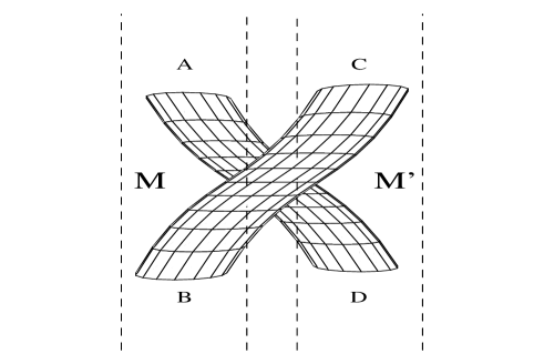
Figure 1: To better visualize the intrinsic geometry of the 3-dimensional KN manifold, the KN disk is drawn as if it presented a finite thickness, and consequently there is a space separation between the upper and lower surfaces of the disk. The left-hand side of each configuration state represents the upper and lower surfaces of the disk in M, whereas the right-hand side represents the upper and lower surfaces of the disk in M’. The lower B surface in M must be joined with the upper C surface in M’, and the lower D surface in M’ must be joined with the upper A surface in M.

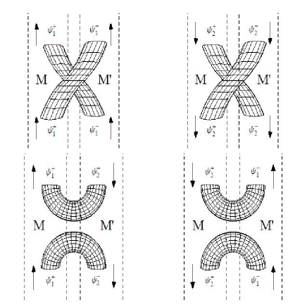
Figure 2: The four possible geometric configurations of KN states for a specific value of the electric charge. The KN disk on each space, that is, on M and on M’, is placed on the $z=0$ plane. The arrows indicate the sense of the spin vector.

By a simple analysis of the structure of the extended KN metric, it is possible to isolate four physically inequivalent states on each side of ${\mathcal{M}}$, that is, on M and M’. These states can be labeled by the sense of rotation ($a$ can be positive or negative), and by the sign of the electric charge (positive or negative). Before a spin rotation axis is chosen, these states are equivalent (up to a rotation) but after choosing it they are physically different. If we place the KN disk in the $xy$ plane of a Cartesian coordinate system, the spin vector will be either in the $+z$ or in the $-z$ direction. Now, each one of these inequivalent solutions in M must be joined continuously through the KN disk to another one in M’, but with opposite charge. Since we want a continuous joining of the metric components, this matching must take into account the sense of rotation of the rings. Through a spatial separation between the upper and lower disks on each manifold, these joinings can be drawn as solid cylinders (see Fig. 1), which makes explicit the difference between both disks. For the sake of simplicity, we are going to consider only one of the two possible electric charges on M ($q<0$, for example). In Fig. 2, the tubular joinings between M and M’, just as in Fig. 1, are drawn, but now taking into account the different spin directions in each disk, which are drawn as small arrows. The only differences between these configurations are the orientation of the spin vector and the geometry of the tubes.

Now, in order to fully understand the topology of the spatial section of the KN spacetime, let us obtain its spatial metric, that is, the metric of its 3- dimensional space section. As the KN metric has non-zero off-diagonal terms, the correct form of the 3-dimensional infinitesimal interval is [15]

$$d\gamma^{2}=\left(-g_{ij}+\frac{g_{oi}g_{oj}}{g_{oo}}\right)dx^{i}\,dx^{j}\equiv\gamma_{ij}\,dx^{i}\,dx^{j},$$ (7)

where $i,j=1,2,3$. Applying this formula to the KN metric (1), we obtain

$$d\gamma^{2} = \left(\frac{r^{2}+a^{2}\cos^{2}\theta}{r^{2}-2mr+a^{2}+q^{2}}\right)dr^{2}+\left(r^{2}+a^{2}\cos^{2}\theta\right)d\theta^{2}$$ (8)

$$+ \left(\frac{(r^{2}+a^{2}\cos^{2}\theta)\sin^{2}\theta}{r^{2}+a^{2}\cos^{2}\theta-2mr+q^{2}}\right)\left(r^{2}+a^{2}-2mr+q^{2}\right)d\phi^{2}.$$

The first thing to notice is that the spatial components are finite in the ring points, that is, $r=0$ and $\theta=\pi/2$. This does not mean that the singularity is absent. Rather, it means that only the metric derivatives are singular, not the metric itself. We can thus conclude that the spatial section of the KN solution has a well defined topology. In fact, the distance function

$$d(p,q)=\int_{p}^{q}\sqrt{\gamma(u)}\;du$$

is easily seen to be finite for any nearby points $p$ and $q$ of the space. The basic conclusion is that the KN space section, or ${\mathcal{M}}^{3}$, has a well defined topological structure, and is consequently a topological space.

In spite of presenting a well defined topological structure, the space ${\mathcal{M}}^{3}$ is not locally Euclidean everywhere. To see that, let us calculate the spatial length ${\mathcal{L}}$ of the border of the disk $r=0$. It is given by

$${\mathcal{L}}=\int_{0}^{2\pi}d\gamma,$$ (9)

where the integral is evaluated at $r=0$ and $\theta=\pi/2$. As a simple calculation shows, it is found to be zero, which means that the border of the disk is topologically a single point of ${\mathcal{M}}^{3}$. Therefore, an open ball centered at the point $r=0$, $\theta=\pi/2$ will not be diffeomorphic to an open Euclidean ball, and consequently the space ${\mathcal{M}}^{3}$ will not be locally Euclidean on the border of the disk $r=0$. This problem can be solved by using Wheeler’s concept of the electric charge. According to his proposal, the electric field lines never end at a point: they are always continuous. It is the non-trivial topology of spacetime which, by trapping the electric field, mimics the existence of charge sources. Applying this idea to the KN solution, we see that the electric field lines end at the singular ring only from the 4-dimensional point of view. From the 3-dimensional point of view, they end at a point (the border of the disk). Now, if this point is not the end of the electric field lines, then they must follow a path to the side with $r$ negative. This situation is quite similar to that of the Reissner-Nordström solution, where the electric field lines can be continued to the negative $r$ side by writing the solution in Kruskal-Szekeres coordinates [10] (it should be noted, however, that in this case the solution is not wholly static since the timelike coordinate changes to spacelike at small distances from the singularity). In the same way as in the Reissner-Nordström solution, we can excise a neighborhood of the point $r=0$ of the KN solution, and join again the resulting borders. In the KN case, considering the values of the electron mass, charge and spin, the time coordinate keeps its timelike nature at all points of the space, so the solution remains stationary after the excision procedure. Furthermore, from the causal analysis of the solution we can choose to excise precisely the torus-like region around the singularity where there exist non-causal closed timelike curves. From the metric (1), it is is easy to see that the coordinate $\phi$ becomes timelike in the region where the following inequality is fulfilled [16]:

$$r^{2}+a^{2}-\left(\frac{q^{2}-2mr}{r^{2}+a^{2}\cos^{2}\theta}\right)a^{2}\sin^{2}\theta<0.$$ (10)

By removing this region, the KN spacetime becomes causal. As already said, this region has a simple form: it is tubular-like and surrounds the singular ring on the negative and positive $r$ sides. When the values of $a$, $q$ and $m$ are chosen to be those of the electron, the surface of the tubular-like region is separated from the singular ring by a distance of the order of $10^{-34}$ cm. At these infinitesimal distances, topology changes are predicted to exist, so it is not unexpected to have changes in the connectedness of spacetime topology. Wheeler’s idea can then be implemented in the KN case. This means to excise the infinitesimal region from the positive and negative $r$ sides, and then glue back the manifold keeping the continuity of both electric field lines and metric components. A simple drawing of the region to be excised can be seen in Fig. 3, where the direction of the gradient of $r$ has been drawn at several points, and the region’s size has been greatly exaggerated.

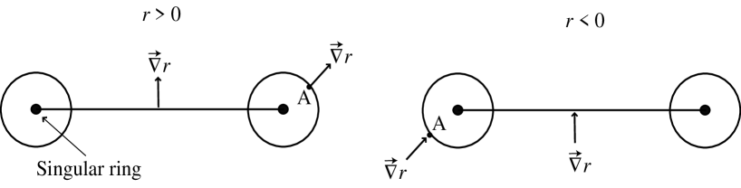
Figure 3: Tubular-like regions around the singular ring, which is to be excised. Several $\vec{\nabla}r$ directions are also depicted, which show how the borders in the positive and negative $r$ sides can be continuously glued.

As an example, note that the point $A$ on the positive $r$ side must be glued to the point $A$ on the negative $r$ side. If we continue to glue all points of the tubular border, we obtain a continuous path for the electric field lines that flow from one side of the KN solution to the other side. Wheeler’s idea is then fully implemented, yielding a 3-dimensional spatial section ${\mathcal{M}}^{3}$ which is everywhere locally Euclidean, and consequently a Riemannian manifold.

For the sake of completeness, we determine now the form of the surface obtained by joining the points of the tubular borders in a metric-continuous way. To do it, we must define the application ${\cal A}:S^{1}\rightarrow S^{1}$, which is constructed in the following way: draw the two $S^{1}$ of Fig. 3, but now centered at the points $(a,0,0)$ and $(-a,0,0)$ of a Cartesian coordinate system. The application ${\cal A}(p\in S^{1})$ is then defined as ${\cal A}(x,0,z)=(-x,0,-z)$, where $(x,0,z)$ are the coordinates of $p$. The form of this application is deduced from the restriction of joining the tubular borders in a metric-continuous way. The surface determined by the joinings is then generated by the quotient space of $S^{1}$ by the equivalence relation $p\sim{\cal A}(p)$, and by a rotation of $\pi$ of the circles around $z$. This surface coincides with the well known Klein Bottle (denoted by $U_{2}$), as can be easily verified in Ref. [17]. It is important to remark that the Klein bottle has also been found by Punsly [18] in the context of the Kerr solution, through a metric extension procedure which eliminates the singular ring. However, in our case we have a physical justification for the excision procedure: the continuity of the electric field lines.

The elimination of the singular ring can be better understood by considering the map $r\rightarrow e^{r}$, which makes possible to see both sides of the $r=0$ surface. This map is shown in Fig. 4, with the circles representing the small excised neighborhoods around the ring singularity. The full picture of the resulting $3$-manifold is obtained by rotating the plane of the figure by $\pi$. It is clear from this figure that the resulting manifold will be multiple connected since any path encircling the excised region cannot be contracted to a point. The borders of the excised regions must be joined in such a way to make the radial component of the metric continuous, as discussed in the analysis of Fig. 3. The other components of the metric are equal on the excised borders (by rotational symmetry), so that they can be always continuously matched.

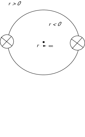
Figure 4: View of the total $2$-dimensional symmetric section of ${\mathcal{M}}^{3}$ obtained through the map $r\rightarrow e^{r}$. The big circle represents the surface $r=0$. The ring singularity is located in the equator, and the small circles represent the infinitesimal regions to be excised around the singularity.

According to the above construction, ${\mathcal{M}}^{3}$ is a non-trivial differentiable three-manifold. This three-manifold can be seen as a connected sum of the form

$${\mathcal{M}}^{3}=\mathbf{R}^{3}\sharp\mathbf{K}^{3}\sharp\mathbf{R}^{3},$$ (11)

where the first $\mathbf{R}^{3}$ represents the asymptotic space section of M, the second $\mathbf{R}^{3}$ represents the asymptotic space section of M’, and the 3-space $\mathbf{K}^{3}$ is the manifold formed by the one-point compactification of ${\mathcal{M}}^{3}$, which is obtained by adding the two points at $\{-\infty,\infty\}$. Then, each 2-sphere, respectively at $\pm\infty$, must be taken as a point of $\mathbf{K}^{3}$. If the connection between the disks were removed, $\mathbf{K}^{3}$ would become homotopic to two disjoint $3$-spheres. This comes from the fact that $\mathbf{R}^{3}\bigcup\{\infty\}\simeq S^{3}$. But, as far as the joinings are present, $\mathbf{K}^{3}$ is not simply connected because there exist loops (those surrounding the $U_{2}$ surface) not homotopic to the identity. In fact, the first fundamental group of $\mathbf{K}^{3}$ is found to be $\pi_{1}(\mathbf{K}^{3})=\mathbf{Z}$. Furthermore, the second fundamental group of $\mathbf{K}^{3}$ is found to be $\pi_{2}(\mathbf{K}^{3})=\{e\}$.

3 Existence of Half-Integral Angular Momentum States

3.1 Topological conditions

In order to exhibit gravitational states with half-integral angular momentum, a $3$-manifold ${\mathcal{M}}^{3}$ must fulfill certain topological conditions. These conditions were stated by Friedman and Sorkin [11], whose results were obtained from a previous work by Hendriks [19] on the obstruction theory in $3$ dimensions. In order to understand Hendrik’s result, it is convenient to divide the manifold ${\mathcal{M}}^{3}$ into an interior (${\mathcal{M}}^{3}_{I}$) and an exterior (${\mathcal{M}}^{3}_{E}$) regions in such a way that ${\mathcal{M}}^{3}_{I}\cap{\mathcal{M}}^{3}_{E}$ is a spherical symmetric shell. After that, one defines a rotation by an angle $\alpha$ of the submanifold ${\mathcal{M}}^{3}_{I}$ with respect to ${\mathcal{M}}^{3}_{E}$ as a three-geometry obtained by cutting ${\mathcal{M}}^{3}_{I}$ at any sphere $S^{2}\subset{\mathcal{M}}^{3}_{I}\cap{\mathcal{M}}^{3}_{E}$, and re- identifying (after rotating) the inner piece with the outer. Then, one looks for a diffeomorphism that takes the final three-geometry, obtained after a rotation of $\alpha=2\pi$, to the initial one, characterized by $\alpha$ equal to $0$. If this diffeomorphism can be deformed to the identity, the gravitational states defined on the manifold can have only integral angular momentum. If the diffeomorphism cannot be deformed to the identity, then half-integral angular momentum gravitational states do exist. This diffeomorphism was called by Hendriks a rotation parallel to the sphere, and it will be denoted by $\rho$.

Hendriks’ results can then be summarized in the following form. If the division into an exterior and interior region is not possible, then $\rho$ cannot be deformed into the identity. Physically, this means that if M and M’ are joined not only at the surface $r=0$, but also at any other place, ${\mathcal{M}}^{3}$ can exhibit half-integral angular momentum states, since in this case there would not exist interior and exterior regions to a shell that encloses the $r=0$ surface. On the other hand, if the division is possible, then ${\mathcal{M}}^{3}$ will exhibit only integral angular momentum states only if it is a connected sum of compact three-manifolds (without boundary),

$${\mathcal{M}}^{3}=\mathbf{R}^{3}\sharp M_{1}\sharp\ldots\sharp M_{k},$$

each of which (a) is homotopic to $P^{2}\times S^{1}$ ($P^{2}$ is the real projective two-sphere), or (b) is homotopic to an $S^{2}$ fiber bundle over $S^{1}$, or (c) has a finite fundamental group $\pi_{1}(M_{j})$ whose two-Sylow subgroup is cyclic. In order to exhibit half-integral angular momentum states, therefore, the 3-manifold ${\mathcal{M}}^{3}$ must fail to fulfill either one of these three conditions.

According to the decomposition (11), ${\mathcal{M}}^{3}$ can be seen as the connected sum of two $\mathbf{R}^{3}$ and $\mathbf{K}^{3}$. Now, as the original analysis of Hendriks was made for compact topological manifolds without boundary, we have to compactify $\mathbf{K}^{3}$ by adding two points at infinity. Besides compact, the resulting 3-space turns out to be without boundary (see Appendix B. Topological Properties of $\mathbf{K}^{3}$). Accordingly, Hendriks results can be used, and we can say that the manifold ${\mathcal{M}}^{3}$ will admit half-integral angular momentum states only if $\mathbf{K}^{3}$ fails to fulfill one of the above conditions (a) to (c). Condition (a) is clearly violated because, as $\pi_{1}(\mathbf{K}^{3})=\mathbf{Z}$, and as

$$\pi_{1}(P^{2}\times S^{1})=\pi_{1}(P^{2})\oplus\pi_{1}(S^{1})=\mathbf{Z}_{2}\oplus\mathbf{Z},$$

$\mathbf{K}^{3}$ cannot be homotopic to $P^{2}\times S^{1}$. Condition (b) is more subtle, but it is also violated. In fact, as is well known [20], the number of inequivalent bundles of $S^{2}$ over $S^{1}$ is just two: A trivial and a non- trivial one. Since the non-trivial bundle is always non-orientable, $\mathbf{K}^{3}$ cannot be homotopic to this space since it is orientable by construction. The trivial bundle $T^{3}$, on the other hand, is formed by taking the direct product of $S^{2}$ with $S^{1}$. We then have

$$\pi_{1}(T^{3})=\pi_{1}(S^{2}\times S^{1})=\pi_{1}(S^{2})\oplus\pi_{1}(S^{1})=\{e\}\oplus\mathbf{Z},$$

which is formally the same as $\pi_{1}(\mathbf{K}^{3})$. However, the second homotopy group of $T^{3}$ is given by

$$\pi_{2}(T^{3})=\pi_{2}(S^{2}\times S^{1})=\pi_{2}(S^{2})\oplus\pi_{2}(S^{1})=\mathbf{Z}\oplus\{e\},$$

and as $\pi_{2}(\mathbf{K}^{3})=\{e\}$, then clearly $\pi_{2}(\mathbf{K}^{3})\neq\pi_{2}(T^{3})$. This shows that $\mathbf{K}^{3}$ cannot be homotopically deformed to a bundle $S^{2}$ over $S^{1}$. Finally, as discussed in the last section, condition (c) is also violated because the fundamental group $\pi_{1}(\mathbf{K}^{3})=\mathbf{Z}$ is infinite. We can then conclude that the KN spacetime does admit gravitational states with half-integral angular momentum. More precisely, we can conclude that it admits gravitational states with spin 1/2.

3.2 Behavior under rotations

By using the definition of $\rho$ introduced earlier in this section, we can proceed to analyze the effect of a rotation in the region around $r=0$ of the manifold ${\mathcal{M}}^{3}$. The following analysis apply to anyone of the two possible interpretations, M joined to M’ through $r=0$ only, or through various other points. One has to choose a spherical shell centered on any one of the two sides of the $r=0$ surface. After choosing the shell one must look at the effect of a rotation on the 3-geometry of the manifold. For simplicity, we choose the positive side of de surface $r=0$ centered on a Cartesian coordinates system and a shell centered on $(0,0,0)$ with a radius large enough so that the geometry outside the shell can be taken as flat.

If we perform now a rotation by an angle $\alpha$ around anyone of the axis $x$, $y$ or $z$ of the interior region of the shell, the effect on the 3-geometry is to twist the cylindrical tubes of Fig. 1. In the specific case of a rotation around the $x$ axis, the twist of the tubes is shown in Fig. 5 for $\alpha=\pi$ and $\alpha=2\pi$.

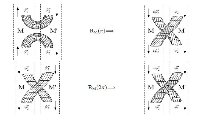
Figure 5: The effect, on the KN states, of rotations around the $x$ axis of the interior region of a shell enclosing $r=0$. The unwitting diffeomorphism can be seen as a dilatation of the tubes that takes them around one of the extreme points of the cylinders.

From this figure, it can be inferred that only after a $4\pi$ rotation the twisting of the tubes can be undone by deforming and taking them around one of their extreme points. In other words, only after a $4\pi$ rotation a diffeomorphism connected to the identity does exist, which takes the metric of the twisted tubes into the metric of the untwisted ones. We mention in passing that the form of this diffeomorphism is equal to the one solving the well-known Dirac’s scissors problem [21].

The effect of a rotation in the interior region of the chosen shell can also be seen by performing first a transformation in the Boyer-Lindquist coordinates that modifies the coordinate $r$ only:

$$(t,r,\theta,\phi)\rightarrow(t,\ln R,\theta,\phi).$$ (12)

This transformation compactifies M’, and takes the points on the disk ($r=0$) into the points on the surface $R=1$. A simplified form of the transformed three manifold ${\mathcal{M}}^{3}$ can be seen in Fig. 6. In this figure, the tubes joining the spaces M and M’ are drawn vertically. They must join the points of the inner surface (except those points near the equator) with the points of the outer surface. The points of M’ are those within the central surface, which is defined by $R=1$. It should be remarked that the homotopy groups of ${\mathcal{M}}^{3}$ are not altered by the transformation.

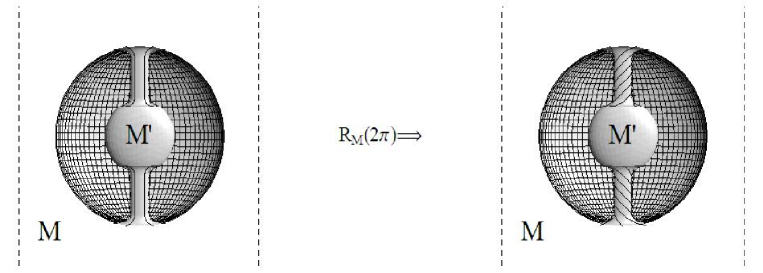
Figure 6: By performing the coordinate transformation $r\rightarrow\ln R$, the KN extended manifold can be represented as depicted in the figure. The central surface represents the points with $R=1$, and M’ is represented by the inner points. The outer surface represents also the points with $R=1$, but seen from the M side. The tubes joining the two spaces are drawn vertically. To the right, it is represented the effect of a $2\pi$ rotation in the interior region of a shell enclosing $r=0$.

Now, a rotation in the interior region of a shell enclosing $r=0$ can be seen as a twisting of the cylindrical tubes that connect the two spaces. For a rotation by an angle $\alpha=2\pi$, this twisting cannot be undone by a diffeomorphism homotopic to the identity, since the extreme points of the cylinder should be kept fixed for it to be connected to the identity. For a rotation by an angle $\alpha=4\pi$, however, it is possible to untwist them because in this case there exists a diffeomorphism homotopic to the identity that untwist them, and at the same time keeps the extreme points fixed. The form of this unwitting diffeomorphism can be found in page 309 of ref. [10]. The fact that the topological structure of the spatial section of the KN manifold returns to its initial state after a $4\pi$ rotation is a more intuitive way to see that this space admits spinorial states.

4 Algebraic Representation of the KN States

4.1 Spinor states

Following Ref. [11], we denote by $\Upsilon({\mathcal{M}}^{3})$ the space of asymptotically flat positive-definite three-metrics $g_{ab}$ on ${\mathcal{M}}^{3}$. Since the metric on ${\mathcal{M}}^{3}$ is fixed (up to a diffeomorphism), different points in $\Upsilon({\mathcal{M}}^{3})$ represent three-metrics which differ only by the geometry of the joining between the sides of the $r=0$ surface. We define a state vector $\psi$, in the Schrödinger picture, as a functional on the space $\Upsilon({\mathcal{M}}^{3})$. The generalized position operator $\widehat{g}_{ab}$ is then defined as

$$\widehat{g}_{ab}\psi(g)=g_{ab}\psi(g),$$ (13)

which means that, for every point of $\Upsilon({\mathcal{M}}^{3})$, we have a different state vector $\psi(g)$. Now, from the discussion of the last section, we can say that (under rotations) a path in $\Upsilon({\mathcal{M}}^{3})$ is closed if and only if the parameter of the path varies from $0$ to $4\pi$. Furthermore, since the points of $\Upsilon({\mathcal{M}}^{3})$ are in one to one correspondence with the states $\psi(g)$, we find that the effect of a $2\pi$ rotation on $\psi(g)$ is not equal to the identity operation:

$$\widehat{R}(2\pi)\psi(g)=\psi(R(2\pi)g)=\psi(g^{\prime}\neq g)\neq\psi(g).$$

An adequate linear representation for the states $\psi(g)$ is one that carries, in addition to the informations about mass and charge, also information on the non- trivial behavior under rotations of the states representing the KN solution. As the state $\psi(g)$ depends on the metric $g_{ab}$, it is not a simple task to infer its general form. As a first step, we can separate a general $\psi(g)$ into a part ($\psi^{+}$) defined on the positive $r$ coordinates, and another ($\psi^{-}$) defined on the negative $r$ coordinates:

$$\psi=a_{+}\psi^{+}+a_{-}\psi^{-}.$$ (14)

Furthermore, if we choose the spin direction along the $z$-axis, we have two possibilities for it (see Fig. 2). Therefore, we can write

$$\psi^{+} = b_{1}\psi^{+}_{1}+b_{2}\psi^{+}_{2}$$ (15)

$$\psi^{-} = c_{1}\psi^{-}_{1}+c_{2}\psi^{-}_{2}.$$ (16)

This superposition is necessary because only after a measurement of the spin direction we know for sure the sign of $a$ in the metric (1). Replacing (15) and (16) into (14), we obtain

$$\psi=a_{+}\left(b_{1}\psi^{+}_{1}+b_{2}\psi^{+}_{2}\right)+a_{-}\left(c_{1}\psi^{-}_{1}+c_{2}\psi^{-}_{2}\right).$$ (17)

We want also that the state $\psi(g)$ be an eigenvector of both the energy and the spin operators. This means that

$$S_{z}\psi^{\pm}_{1} = s_{z}\psi^{\pm}_{1}=\frac{1}{2}\psi^{\pm}_{1}$$ (18)

$$S_{z}\psi^{\pm}_{2} = s_{z}\psi^{\pm}_{2}=-\frac{1}{2}\psi^{\pm}_{2}$$ (19)

$$H\psi^{+} = -i\partial_{t}\psi^{+}=m\psi^{+}$$ (20)

$$H\psi^{-} = -i\partial_{t}\psi^{-}=-m\psi^{-}$$ (21)

where $S_{z}$ is the spin operator along the $z$ direction, $H$ is the energy operator, and $m$ is the mass of the KN solution. In these relations we have implicitly used the correspondence between mass and energy (remember that $m$ is negative on the negative $r$ sector of ${\mathcal{M}}^{3}$).

Now, as a consequence of the fact that an observer in the positive $r$ side of $r=0$, as well as one in the negative $r$ side, sees a state vector that transforms into itself only after a $4\pi$-rotation, we can naturally represent these states in a spinor basis of the Lorentz group SL(2, $\mathbf{C}$). More specifically, each one of the four inequivalent states defined in the positive $r$ side can be taken as Weyl spinors transforming under the $({1}/{2},0)$ representation, and those defined in the negative $r$ side as Weyl spinors transforming under the $(0,{1}/{2})$ representation of the Lorentz group (see Appendix A. Lorentz Group and Parity Transformations for a more detailed discussion). Furthermore, according to Eqs. (20) and (21), the linear representation for $\psi$ must also contain a part proportional to a complex exponential of energy multiplied by time. Finally, it is important to notice that the representation cannot mix $\psi^{+}$ and $\psi^{-}$ as they are defined on different spatial regions. With these provisos, we are led to the following representation for $\psi(g)$:

$$\psi(g)=a_{+}\left[b_{1}e^{iEt}\left(\begin{array}[]{c}1\\ 0\\ 0\\ 0\end{array}\right)+b_{2}e^{iEt}\left(\begin{array}[]{c}0\\ 1\\ 0\\ 0\end{array}\right)\right]+a_{-}\left[c_{1}e^{-iEt}\left(\begin{array}[]{c}0\\ 0\\ 1\\ 0\end{array}\right)+c_{2}e^{-iEt}\left(\begin{array}[]{c}0\\ 0\\ 0\\ 1\end{array}\right)\right].$$ (22)

This can be considered as the most simple linear representation of a general $\psi(g)$ associated with the KN solution (at rest).

4.2 Evolution equation

If we want the above solution to represent a particle, we need it to be an eigenstate of momentum (or position). This is not easy because the “position” of the “particle” is not defined by a simple point in spacetime. So, for example, the usual momentum operator $-i\vec{\nabla}$ is of no use because it is defined for point-like particles. To solve this problem, we need to get an approximate representation for $\psi(g)$, valid in the limit of long distances from the singularity. In this limit, the KN solution is supposed to converge to the metric produced by a spinning structureless point particle. Only in this case the momentum operator $-i\vec{\nabla}$ becomes well suited for defining the momentum of the particle. In this limit, we can also consider the background metric as flat, which means to consider $\eta_{\mu\nu}={\rm diag}(-1,1,1,1)$ as the spacetime metric. Using the form of $\psi(g)$ as given by Eq. (22), we find that an adequate dependence on the momentum of the particle is given by the exponential $i\vec{p}\cdot\vec{x}$. This is due to the fact that, in this case, the two exponential factors combine to give a covariant expression, and at the same time the state becomes an eigenvector of momentum. The most general state $\psi_{p}(g)$ is then given by

$$\psi_{p}(g)=a_{+}e^{-ip_{\mu}x^{\mu}}\left[b_{1}\left(\begin{array}[]{c}1\\ 0\\ 0\\ 0\end{array}\right)+b_{2}\left(\begin{array}[]{c}0\\ 1\\ 0\\ 0\end{array}\right)\right]+a_{-}e^{ip_{\mu}x^{\mu}}\left[c_{1}\left(\begin{array}[]{c}0\\ 0\\ 1\\ 0\end{array}\right)+c_{2}\left(\begin{array}[]{c}0\\ 0\\ 0\\ 1\end{array}\right)\right].$$ (23)

Now, from Eqs. (20) and (21), we can write the evolution equation for the KN state as

$$\frac{1}{i}\partial_{t}\psi_{p}=H\psi_{p}\equiv E\left(\begin{array}[]{cc}I_{2}&0\\ 0&-I_{2}\end{array}\right)\psi_{p}\equiv E\,\beta\,\psi_{p},$$ (24)

where $I_{2}$ is the $2\times 2$ identity matrix. The minus sign of the lower components is a reflection of the fact that the lower components of the vector state have negative energy. A more convenient form of the evolution equation can be obtained by performing a unitary transformation. We write this transformation, which is a particular case of the well known Foldy- Wouthuysen transformation [22], in the form

$$\mathbf{U}=\sqrt{\frac{E+m}{2E}}\;\left(\begin{array}[]{cc}I_{2}&-\frac{\sigma_{i}p_{i}}{E+m}\\ \frac{\sigma_{i}p_{i}}{E+m}&I_{2}\end{array}\right).$$ (25)

It can then be easily verified that

$$\Psi_{p}=\mathbf{U}\;\psi_{p}$$ (26)

is a solution of the modified evolution equation

$$\frac{1}{i}\partial_{t}\Psi_{p}=\mathbf{H}\,\Psi_{p}\equiv\left(\alpha_{i}p_{i}+\beta m\right)\Psi_{p},$$ (27)

with

$$\mathbf{H}=\mathbf{U}H\mathbf{U}^{\dagger}$$ (28)

the transformed Hamiltonian. As is well known, Eq. (27) is the standard form of Dirac’s relativistic equation for the electron. The basic conclusion is that the KN solution of Einstein’s equation can be represented by a state vector that is a solution of the Dirac equation. Besides exhibiting all properties of a solution of the Dirac equation, the KN state provides an intuitive explanation for mass, spin and charge. Furthermore, it clarifies the fact that, during an interaction, both positive and negative energy states contribute to the solution of the Dirac equation. This means that it is not possible to describe interacting states as purely positive or purely negative energy states since, as the extended KN solution explicitly shows, the two energy states are topologically linked. On the other hand, it is possible to describe a free, moving, positive-energy (negative-energy) state without considering negative-energy (positive-energy) components. It should be remarked that there exists an arbitrariness in this terminology. In fact, what we call a negative- energy state and a positive-energy state depends on which side of the KN solution we are supposed to live in. Furthermore, as the electric charge enters quadratically in the KN metric, it is not possible to say in which side of the KN solution an ideal observer is, and consequently what we call positive or negative energy state is also a matter of convention.

5 Some Phenomenological Tests

We look now for some experiments where the effects of the singularity would become manifest. We begin by noticing that, for symmetry reasons, the electric dipole moment of the KN solution vanishes identically, a result that is within the limits of experimental data [23]. Another important point is that the uncertainty principle precludes one to localize the electron in a region smaller than its Compton wavelength without producing virtual pairs originated from the large uncertainty in the energy. Since we are proposing an extended electron model with the size of its Compton wavelength, the question then arises whether it contradicts scattering experiments that gives a limit to the extendedness of the electron as smaller than $10^{-18}$cm. This is a difficult question because this model describes the electron as a nontrivial topological structure with a trapped electromagnetic field. As a consequence, its interaction with other electrons must be governed by the coupled Einstein–Maxwell equations. Even though, a simplified answer to this question can be given by noticing that a boost (in the spin direction) transforms the Kerr–Newman parameters $m$ and $a$ according to [24]

$$a^{\prime}=a\sqrt{1-v^{2}};\qquad m^{\prime}=\frac{m}{\sqrt{1-v^{2}}},$$ (29)

where $v$ is the boost velocity. It should be clear that $a$ and $m$ are thought of as parameters of the KN solution, which only asymptotically correspond respectively to angular momentum per unit mass and mass. Near the singularity, $a$ represents the radius of the singular ring, which according to Carter is unobservable [16]. The above “renormalization” of the KN parameters has been discussed by many authors [25], being necessary to maintain the internal angular momentum constant. As a consequence, to a higher velocity, there might correspond a smaller radius of the singular ring. With this renormalization, it is a simple task to verify that, for the usual scattering energies, the resulting radius is within the experimental limit for the extendedness of the electron. According to these arguments, therefore, the electron extendedness will not show up in high-energy scattering experiments. This extendedness will show up only in low energy experiments, where the electrons move at low velocities.

Let us then look for a simple low energy test involving interactions with other particles, or electromagnetic fields. Take, for example, a pair of electrons confined to a two dimensional plane $D$. If a strong magnetic field perpendicular to the plane is applied, the spin vectors of the electrons will align with the magnetic field. This means that the KN disk will be coplanar with $D$. The magnetic flux $\Phi$ through the plane is given by

$$\Phi=\int_{D}{\vec{B}\cdot d\vec{s}}=\int_{D}{\vec{\nabla}\times\vec{A}(z)\cdot d\vec{s}}=\oint_{\partial D}A(z)dz,$$ (30)

where $\vec{B}$ is the magnetic field, $\vec{A}$ is the vector potential defined on $D$, and $z=x+iy$ are complex coordinates for the plane. The border of $D$ will have three parts: An external part, and the border enclosing the KN disk for each electron. Taking periodic boundary conditions on the external border, we are left with two disconnected borders only. In such multiply-connected spacetime, the vector potential $\vec{A}(z)$ is not uniquely defined since there exist two other closed one-forms $\zeta_{k}^{-1}d\zeta_{k}$, $k=1,2$, with the property [26]

$$\int_{\partial D_{k}}\zeta_{k}^{-1}d\zeta_{k}=2\pi i,$$ (31)

where $\partial D_{k}$ denotes the boundary of each electron disk. Due to this fact, the computation of the flux (30) must take into account all different configurations for $\vec{A}(z)$ [27]. Assuming that all three configurations enter with the same weight, and using unities in which $q=1$ (so that the flux quanta becomes $\Phi_{0}=1$), the total flux turns out to be

$$\Phi=\oint_{\partial D_{1}\cup\partial D_{2}}A(z)dz+\oint_{\partial D_{1}\cup\partial D_{2}}\left(A(z)dz-\frac{i}{4\pi}\zeta_{1}^{-1}d\zeta_{1}-\frac{i}{4\pi}\zeta_{2}^{-1}d\zeta_{2}\right)$$

$$+\oint_{\partial D_{1}\cup\partial D_{2}}\left(A(z)dz-\frac{i}{4\pi}\zeta_{1}^{-1}d\zeta_{1}\right)+\oint_{\partial D_{1}\cup\partial D_{2}}\left(A(z)dz-\frac{i}{4\pi}\zeta_{2}^{-1}d\zeta_{2}\right).$$ (32)

Using then the flux quantization condition

$$\oint_{\partial D_{1}\cup\partial D_{2}}A(z)\,dz=n;\quad n=1,2,\dots,$$ (33)

we get

$$\Phi=4n-2.$$ (34)

If we compute now the relation $\nu=$ number of electrons/number of flux quanta, we get

$$\nu=\frac{2}{4n-2}=\frac{1}{2n-1}.$$ (35)

This experimental setup is used in the study of the Fractional Quantum Hall Effect (FQHE) [28], and in this context the quantity $\nu$ is called the filling factor. The above result coincides with the experimental one if we consider that the interactions between electrons on the confining plane are pair-dominated [29].

6 Conclusions

We have shown in this paper that, by using the extended spacetime interpretation of Hawking and Ellis together with Wheeler’s idea of charge without charge, the KN solution exhibits properties that are quite similar to those presented by an electron, paving the way for the construction of an electron model [30]. The first important point is that, due to its topological structure, the extended KN solution admits the presence of spacetime spinorial structures. As a consequence, the KN solution can naturally be represented in terms of spinor variables of the Lorentz group SL(2, $\mathbf{C}$). The evolution of the KN state vector so obtained is then shown to be governed by the Dirac equation. Another important point is that this model provides a topological explanation for the concepts of mass, charge and spin. Mass can be interpreted as made up of gravitation, as well as rotational and electromagnetic energies, since all of them enter its definition. Charge, on the other hand, is interpreted as arising from the multi- connectedness of the spatial section of the KN solution. In fact, according to Wheeler, from the point of view of an asymptotic observer, a trapped electric field is indistinguishable from the presence of a charge distribution in spacetime. Finally, spin can be consistently interpreted as an internal rotational motion of the infinitesimally sized $U_{2}$ surface. Besides these properties, we have also shown that this model can provide explanations to not well-understood phenomena of solid state physics, as for example the fractional quantum Hall effect. It is important to remark once more that the topology ensued by the Hawking and Ellis interpretation of the Kerr-Newman solution leads actually to fundamental states with spin 1/2 only. Observe, for example, that the Kerr-Newman solution presents four independent states, a typical property of the electron- positron system. Notice, however, that it is possible to construct states with higher spins by considering composed states, with the spin 1/2 solution as building blocks. This, of course, changes the topology of the whole solution. Higher-spin states are therefore possible, but then the manifold $\mathcal{M}$ will exhibit a different topology from the presented here. Finally, we would like to remark that the metric does not fix the sign of $r$ at each side of the $r=0$ surface. It is actually a matter of convention, an arbitrary choice of the observer.

Appendix A. Lorentz Group and Parity Transformations

As is well known, the complexified Lie algebra of the Lorentz group SL(2, $\mathbf{C}$) is isomorphic to the complexified Lie algebra of the group SU(2) $\otimes$ SU(2). In fact, denoting by $J_{i}$ and $K_{i}$ respectively the generators of infinitesimal rotations and boost transformations in M, with $i,j,k=x,y,z$, the complex generators

$$A_{i}=\frac{1}{2}\left(J_{i}+iK_{i}\right)\quad{\rm and}\quad A^{\dagger}_{i}=\frac{1}{2}\left(J_{i}-iK_{i}\right)$$ (36)

are known to satisfy, each one, the SU(2) Lie algebra [31]:

$$\left[A_{i},A_{j}\right] = i\,\epsilon_{ijk}\,A_{k}$$

$$\left[A^{\dagger}_{i},A^{\dagger}_{j}\right] = i\,\epsilon_{ijk}\,A^{\dagger}_{k}.$$

Furthermore, they satisfy also

$$\left[A_{i},A^{\dagger}_{j}\right]=0,$$ (37)

which shows that they are independent, or equivalently, a direct product. The two Casimir operators $A_{i}A_{i}$ and $A_{i}^{\dagger}A_{i}^{\dagger}$ are also known to present respectively eigenvalues $n(n+1)$ and $m(m+1)$, with $n,m=0,1/2,1,3/2,\dots$. Thus, each representation can be labeled by the pair $(n,m)$. Now, as a simple inspection shows, under a parity transformation,

$$J_{i}\rightarrow J_{i}\quad{\rm and}\quad\quad K_{i}\rightarrow-K_{i}.$$ (38)

Therefore, the generators $A_{i}$ and $A_{i}^{\dagger}$ are easily seen to be related by a parity transformation [31].

On the other hand, it is clear from the KN metric (1) in M, which is written in terms of the coordinates $(t,r,\theta,\phi)$, that the KN solution in M’ is written in terms of $(t,-r,\theta,\phi)$. Then, the gradient function $\nabla r$ changes sign in M’, making its Cartesian coordinate system, with origin in the center of the disk, to present negative unitary vectors. This is so because the unitary Cartesian vectors are perpendicular to the $r$ = constant surfaces. The two sides of the KN solution, therefore, are related by a parity transformation. The conclusion is that the relationship between M and M’ is the same as that between $A_{i}$ and $A_{i}^{\dagger}$. This justifies the use in M of Weyl spinors transforming under the $(1/2,0)$ representation, and the use in M’ of Weyl spinors transforming under the $(0,1/2)$ representation of the Lorentz group.

Appendix B. Topological Properties of $\mathbf{K}^{3}$

Let $F:{\mathcal{M}}^{3}\cup\{\pm\infty\}\longrightarrow\mathbf{R}^{3}\cup\{\infty\}$ be a function from the metric space ${\mathcal{M}}^{3}$ (plus two points at infinity) to a 3-dimensional Euclidean space (plus one point at infinity). The function is defined by:

$$F(r,\theta,\phi) = (e^{r},\theta,\phi)$$

$$F(-\infty,\theta,\phi) = (0,\theta,\phi)$$

$$F(\infty,\theta,\phi) = (\infty,\theta,\phi).$$

The space $\mathbf{R}^{3}\cup\{\infty\}$ is the Alexandroff’s one-point compactification of $\mathbf{R}^{3}$, which is topologically equivalent to $S^{3}$. The function $F$ takes the surface $r=0$ of the KN solution into a sphere of unit radius, centered at $(0,0,0)$. The singular ring is mapped into the equator of the sphere. The function $F$ is continuous at any point $c\in{\mathcal{M}}^{3}\cup\{\pm\infty\}$ if for any positive real number $\varepsilon$, there exists a positive real number $\delta$ such that for all $p\in{\mathcal{M}}^{3}\cup\{\pm\infty\}$ satisfying $d_{\gamma}(p,c)<\delta$, the inequality $d_{\eta}(F(p),F(c))<\varepsilon$ is also satisfied. As the distance function defined by the metric $\gamma_{ij}$ of ${\mathcal{M}}^{3}$, given by (7), is finite everywhere, the continuity condition is valid for every $p\in{\mathcal{M}}^{3}$. However, as the border of the disk $r=0$ is a single point of ${\mathcal{M}}^{3}\cup\{\pm\infty\}$, the function is not one-to-one. In fact, the point ($r=0$, $\theta=\pi/2$) is mapped into the equator of the unit sphere. Now, since $S^{3}$ is compact, and $F^{-1}$ is continuous, ${\mathcal{M}}^{3}\cup\{\pm\infty\}$ is also compact. If we excise an open set from $S^{3}$ in the form of a solid torus (without boundary) around the equator of the unitary sphere, we are left with a closed subset of $S^{3}$. This closed subset is also compact and has as boundary a 2-dimensional torus $T^{2}$. Denoting by $T^{3}$ the solid torus and by $T_{F}^{3}$ its image under $F^{-1}$, the function

$$(F^{-1})^{\prime}:\mathbf{R}^{3}\cup\{\infty\}-T^{3}\longrightarrow{\mathcal{M}}^{3}\cup\{\pm\infty\}-T_{F}^{3}$$

is found to be continuous. As a consequence, ${\mathcal{M}}^{3}\cup\{\pm\infty\}-T_{F}^{3}$ will also be compact. Now, let $(\alpha,\beta)$ be the coordinates of $T^{2}=S^{1}\times S^{1}$, and consider the map $A:T^{2}\longrightarrow T^{2}$ defined by $A(\alpha,\beta)=(\alpha+\pi,\beta+\pi)$. The surface obtained by making $A(p)\sim p$, and then by taking the quotient space $T^{2}/A$, is the Klein bottle $U_{2}$. In this way, every point $p$ of $U_{2}$ has a neighborhood in $S^{3}$ which is homeomorphic to a Euclidean open ball. This implies that $\{\mathbf{R}^{3}\cup\{\infty\}-T^{3}\}/A$ is a compact manifold without boundary. Therefore,

$${\mathcal{F}}:\{\mathbf{R}^{3}\cup\{\infty\}-T^{3}\}/A\longrightarrow\{{\mathcal{M}}^{3}\cup\{\pm\infty\}-T_{F}^{3}\}/\{(F^{-1})^{\prime}\circ(A)\}=\mathbf{K}^{3}$$

will be a continuous function from a compact space, which means essentially that $\mathbf{K}^{3}$ is also a compact space. Furthermore, since $\mathcal{F}$ is continuous, it maps every open set of $\{\mathbf{R}^{3}\cup\{\infty\}-T^{3}\}/A$ into an open set of $\mathbf{K}^{3}$, which implies that $\mathbf{K}^{3}$ has no boundary: $\partial\mathbf{K}^{3}=0$.

References

- [1] Kerr, R. P. (1963). Phys. Rev. Lett. 11, 237.
- [2] Newman, E. T., and Janis, A. I. (1965). J. Math. Phys. 6, 915.
- [3] Newman, E. T. et al (1965). J. Math. Phys. 6, 918.
- [4] Hawking, S. W., and Ellis, G. F. R. (1973). The Large Scale Structure of Space-Time (Cambridge University Press, Cambridge) p. 161.
- [5] Lopez, C. A. (1984). Phys. Rev. D30, 313; Lopez, C. A. (1992). Gen. Rel. Grav. 24, 285.
- [6] Israelit, M., and Rosen, N. (1995). Gen. Rel. Grav. 27, 153.
- [7] Israel, W. (1970). Phys. Rev. D2, 641.
- [8] Barut, A. O., and Bracken, A. J. (1981). Phys. Rev. D23, 2454.
- [9] Barut, A. O., and Thacker, W. (1985). Phys. Rev. D31, 1386.
- [10] Wheeler, J. A. (1962). Geometrodynamics (Academic Press, New York).
- [11] Friedman, J. L., and Sorkin, R. (1980). Phys. Rev. Lett. 44, 1100.
- [12] Wald, R. M. (1984). General Relativity (The University of Chicago Press, Chicago) p. 289.
- [13] Komar, A. (1959). Phys. Rev. 113, 934.
- [14] Ohanian, H., and Ruffini, R. (1994). Gravitation and Spacetime (Norton & Company, New York) p. 396.
- [15] Landau, L. D., and Lifshitz, E. M. (1975). The Classical Theory of Fields (Pergamon, Oxford).
- [16] Carter, B. (1968). Phys. Rev. 174, 1559.
- [17] do Carmo, M. P. (1976). Differential Geometry of Curves and Surfaces (Prentice-Hall, New Jersey).
- [18] Punsly, B. (1987). J. Math. Phys. 28, 859.
- [19] Hendriks, H. (1977). Bull. Soc. Math. France Memoire 53, 81; see §4.3
- [20] Steenrod, N. (1974). The Topology of Fibre Bundles (Princeton University Press, New Jersey) p. 134.
- [21] Penrose, R., and Rindler, W. (1984). Spinors and Spacetime, Vol. 1 (Cambridge University Press, Cambridge) p. 43.
- [22] Gross, F. (1993). Relativistic Quantum Mechanics and Field Theory (Wiley, New York) p. 147.
- [23] Commins, E. D. et al (1994). Phys. Rev. A50, 2960.
- [24] Burinskii, A., and Magli, G. (2000). Phys. Rev. D61, 044017.
- [25] Luosto, C. O., and Sanchez, N. (1992). Nucl. Phys. B383, 377.
- [26] Petry, H. R. (1979). J. Math. Phys. 20, 231.
- [27] Avis, S. J., and Isham, C. J. (1979). Nucl. Phys. B156, 441.
- [28] Verlinde, E. (1992). Quantum Hall Effect, ed. by M. Stone (World Scientific, Singapore).
- [29] Asselmeyer, T., and Keiper, R. (1995). Ann. Phys. (Lpz) 4, 739; Asselmeyer, T., and Hess, G. (1995). Fractional Quantum Hall Effect, Composite Fermions and Exotic Spinors (cond-mat/9508053).
- [30] Burinskii, A. (2003). Phys. Rev. D68, 105004.
- [31] Ramond, P. (1989). Field Theory: A Modern Primer, 2nd edition (Addison- Wesley, Redwood).