The mass gap and vacuum energy of
the Gross-Neveu model via the $2PPI$ expansion

Abstract

We introduce the $2PPI$ (2-point-particle-irreducible) expansion, which sums bubble graphs to all orders. We prove the renormalizibility of this summation. We use it on the Gross-Neveu model to calculate the mass gap and vacuum energy. After an optimization of the expansion, the final results are qualitatively good.

I Introduction

The Gross-Neveu (GN) model Gross is plagued by infrared renormalons. The origin of this problem lies in the fact that we perturb around an instable (zero) vacuum. A remedy would be the mass generation of the particles, connected to a non-perturbative, lower value of the vacuum energy. Such a dynamical mass must be of a non-perturbative nature, since the GN Lagrangian possesses a discrete chiral symmetry. A dynamical mass is closely related to a nonzero vacuum expectation value (VEV) for a local composite operator $\left(\textrm{i.e. }\overline{\psi}\psi\right)$. This condensate introduces a mass scale into the model. We consider GN because the exact mass gap Forgacs and vacuum energy Zamo are known. This allows a test for the reliability of approximative frameworks before attention is paid to dynamical mass generation in more complex theories like SU($N$) Yang-Mills Verschelde1 . The last few years, several methods have been proposed to solve this problem and get non-perturbative information out of the model Arvanitis ; Verschelde3 ; Karel .
In this paper, we address another approach, the so-called $2PPI$ expansion. Its first appearance and use for analytical finite temperature research can be found in Verschelde4 ; Verschelde5 ; Verschelde6 ; Verschelde7 ; Baacke . In Sec.II, we give a new derivation of the expansion. Sec.III is devoted to the renormalization of the $2PPI$ technique. Preliminary numerical results, using the $\overline{MS}$ scheme, are presented in Sec.IV. We recover the $N\rightarrow\infty$ approximation, but we encounter the problem that the coupling is infinite. In Sec.V we optimize the $2PPI$ technique. We rewrite the expansion in terms of a scheme and scale independent mass parameter $M$. The freedom in coupling constant renormalization is reduced to a single parameter $b_{0}$ by a reorganization of the series. We discuss how to fix $b_{0}$. Numerical results can be found in Sec.VI. We also give some evidence to motivate why results are acceptable. We end with conclusions in Sec.VII.

II The $2PPI$ expansion

We start from the (unrenormalized) GN Lagrangian in two-dimensional Euclidean space time.

$$\mathcal{L}=\overline{\psi}\partial/\psi-\frac{1}{2}g^{2}\left(\overline{\psi}\psi\right)^{2}$$ (1)

This Lagrangian has a global $U(N)$ invariance and a discrete chiral symmetry $\psi\rightarrow\gamma_{5}\psi$ which imposes $\left\langle\overline{\psi}\psi\right\rangle=0$ perturbatively. This model is asymptotically free and has spontaneous chiral symmetry breaking. As such, it is a toy model which mimics QCD in some ways.
First of all, we focus on the topology of vacuum diagrams. We can divide them in 2 disjoint classes:

• Those diagrams falling apart in 2 separate pieces when 2 lines meeting at the same point $x$ are cut. We call those 2-point-particle-reducible or $2PPR$. $x$ is named the $2PPR$ insertion point. FIG.1 depicts the most simple $2PPR$ vacuum bubble.

  

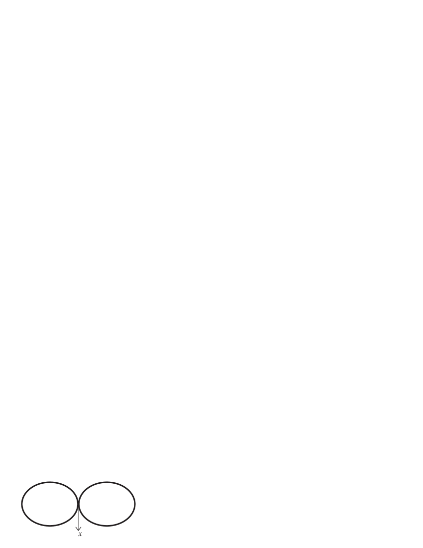
  Figure 1: A $2PPR$ vacuum bubble. $x$ is the $2PPR$ insertion point.

• The other type is the complement of the $2PPR$ class, we baptize such diagrams 2-point-particle-irreducible ($2PPI$) diagrams. FIG.2 shows a $2PPI$ bubble.

  

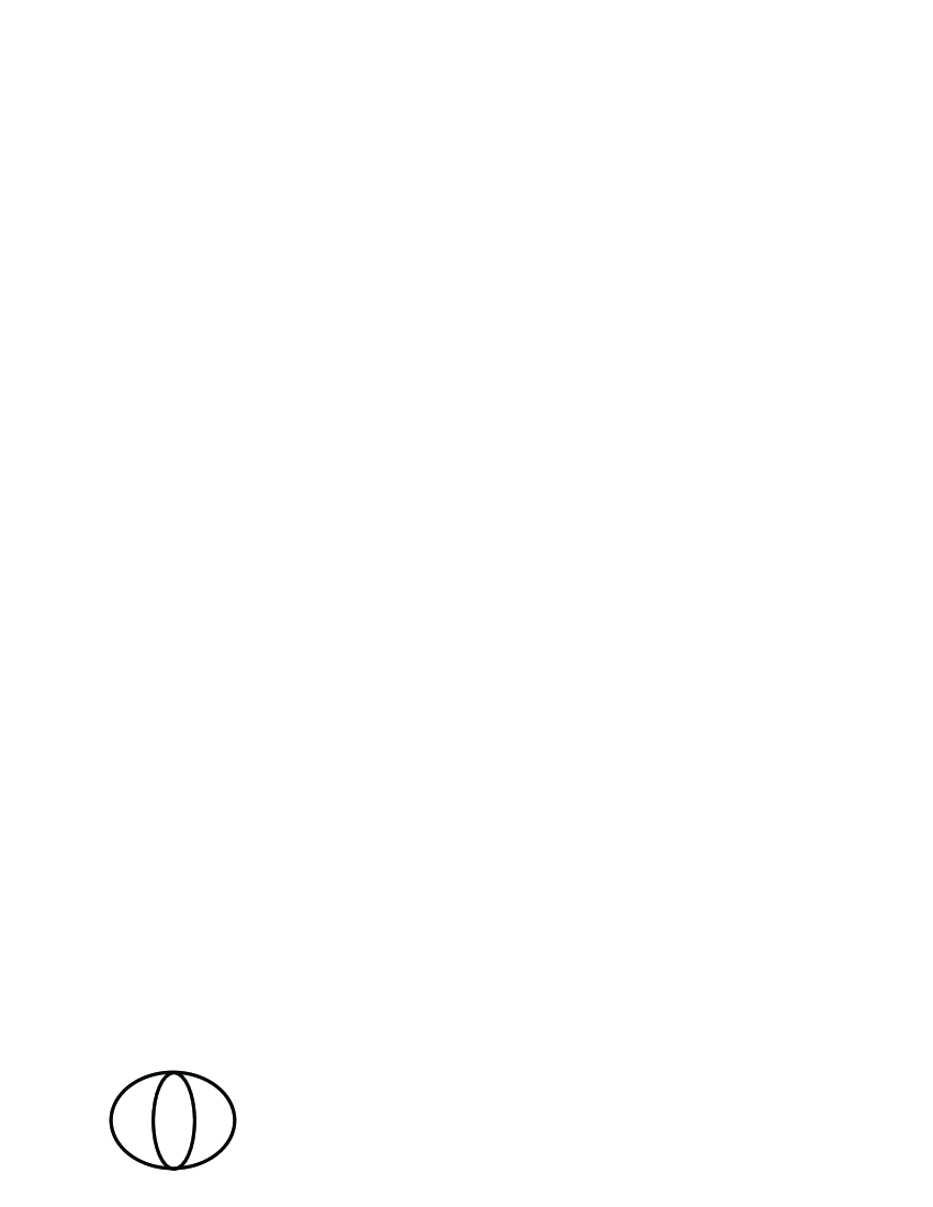
  Figure 2: A $2PPI$ vacuum bubble.

We could now remove all $2PPR$ bubbles from the diagrammatic sum building up the vacuum energy by summing them in an effective mass. To proceed, we must use a little trick. Let’s define

$$\Delta=\langle\overline{\psi}\psi\rangle=\left\langle\overline{\psi}_{i}\psi_{i}\right\rangle$$ (2)

where the index $i=1\ldots 2N$ goes over space as well as internal values. Obviously, we have

$$\Delta_{ij}\equiv\left\langle\overline{\psi}_{i}\psi_{j}\right\rangle=\delta_{ij}\frac{\Delta}{2N}$$ (3)

We now calculate $\frac{dE}{dg^{2}}$ where $E$ is the vacuum energy. The $g^{2}$ derivative can hit a $2PPR$ vertex or a $2PPI$ vertex. (see FIG.3 and FIG.4)

Figure 3: Generic vacuum bubble.

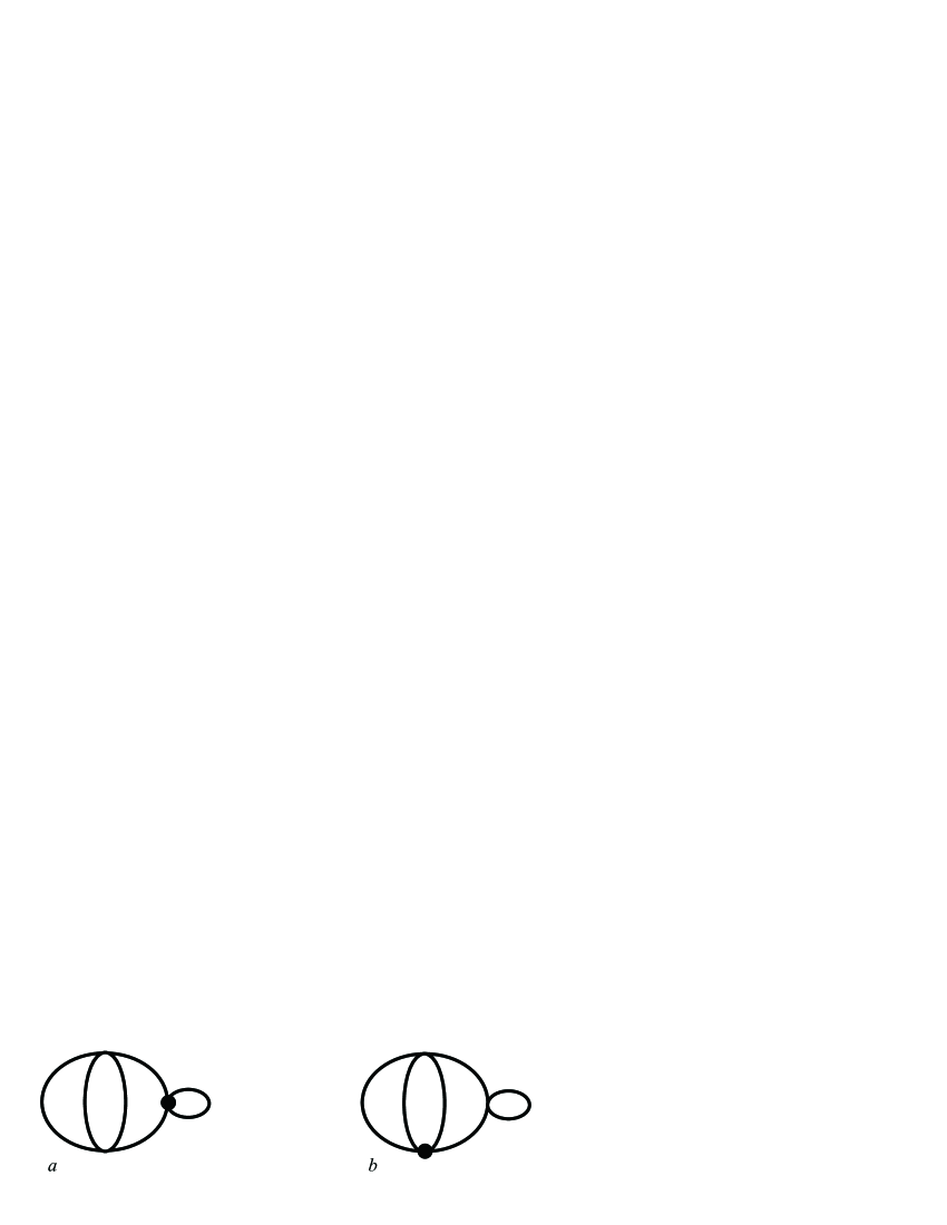
Figure 4: Diagrammatic depiction of $\frac{d}{dg^{2}}$ (fat dot) applied on the bubble of FIG.4.

In the first case, we have diagrammatically the contribution

$$-\frac{1}{2}\Delta_{ij}\left(\delta_{ij}\delta_{kl}-\delta_{il}\delta_{jk}\right)\Delta_{kl}=-\frac{1}{2}\left(1-\frac{1}{2}\right)\Delta^{2}$$ (4)

In the second case, we can unambiguously subdivide the vacuum diagram in one maximal $2PPI$ part, which contains the vertex hit by $\frac{d}{dg^{2}}$, and one or several $2PPR$ parts which can be deleted and replaced by an effective mass $\overline{m}$. A simple diagrammatical argument gives

$$\overline{m}\delta_{ij}=-g^{2}\left(\delta_{ij}\delta_{kl}-\delta_{il}\delta_{jk}\right)\Delta_{kl}$$ (5)

or

$$\overline{m}=-g^{2}\Delta\left(1-\frac{1}{2N}\right)$$ (6)

Summarizing, we have

$$\frac{dE}{dg^{2}}=-\frac{1}{2}\Delta^{2}\left(1-\frac{1}{2N}\right)+\frac{\partial E_{2PPI}}{\partial g^{2}}\left(\overline{m},g^{2}\right)$$ (7)

The $g^{2}$ dependence in $E_{2PPI}$ comes from the $2PPI$ vertices. To integrate (7), we use the Anzatz

$$E\left(g^{2}\right)=E_{2PPI}\left(\overline{m},g^{2}\right)+cg^{2}\Delta^{2}$$ (8)

with $c$ a constant to be determined. Using (6), we find from (8)

$$\frac{dE}{dg^{2}} = \frac{\partial E_{2PPI}}{\partial g^{2}}\left(\overline{m},g^{2}\right)+\frac{\partial E_{2PPI}}{\partial\overline{m}}\left(-\Delta\left(1-\frac{1}{2N}\right)\right.$$ (9)

$$- \left.g^{2}\frac{d\Delta}{dg^{2}}\left(1-\frac{1}{2N}\right)\right)+c\Delta^{2}+2cg^{2}\Delta\frac{d\Delta}{dg^{2}}$$

A simple diagrammatical argument gives

$$\frac{\partial E_{2PPI}}{\partial\overline{m}}\left(\overline{m},g^{2}\right)=\Delta$$ (10)

This is a (local) gap equation, summing the bubble graphs into $\overline{m}$. Using (10) and comparing (9) with (7), we find $c=\frac{1}{2}\left(1-\frac{1}{2N}\right)$, so that we finally have that

$$E\left(g^{2}\right)=\frac{1}{2}g^{2}\left(1-\frac{1}{2N}\right)\Delta^{2}+E_{2PPI}\left(\overline{m},g^{2}\right)$$ (11)

It is easy to show that the following equivalence hold.

$$\frac{\partial E_{2PPI}}{\partial\overline{m}}=\Delta\Leftrightarrow\frac{\partial E}{\partial\overline{m}}=0$$ (12)

One shouldn’t confuse (12) with the usual procedure of minimizing an effective potential $V(\varphi)$ with respect to the field variable $\varphi$. First of all, $\overline{m}$ is not a field variable. Secondly, the expression for $E$ in terms of the $2PPI$ expansion is only correct if the gap equation is fulfilled.

III Renormalization of the $2PPI$ expansion

Up to now, we haven’t paid any attention to divergences. We will now show that an equation such as (11) is valid for the vacuum energy $E$ with fully renormalized and finite quantities. Since in the original Lagrangian there is no mass counterterm, one could naively expect problems with the non-perturbative mass $\overline{m}$, which generates mass renormalization in $E_{2PPI}$. Another possible problem is vacuum energy renormalization. Perturbatively, the vacuum energy is zero and hence no vacuum energy renormalization is needed. Non-perturbatively, we expect logarithmic divergences proportional to $\overline{m}^{2}$ for $E_{2PPI}$. As we will show, both these problems are solved with coupling constant renormalization.

The trick is to separate the contribution of the coupling constant renormalization counterterm $-\frac{1}{2}\delta Z_{4}\left(\overline{\psi}\psi\right)^{2}$ into $2PPR$ and $2PPI$ parts, corresponding with the topology of the original divergent subgraphs. Let $i$ and $j$ be the indices carried by the lines meeting at the $2PPR$ vertex, then we have

$$\delta Z_{4}\left(\delta_{ij}\delta_{kl}-\delta_{il}\delta_{kj}\right)=\delta Z_{4;ij,kl}^{2PPI}+\delta Z_{4;ij,kl}^{2PPR}$$ (13)

Note that crossing will change a $2PPR$ part into a $2PPI$ part.

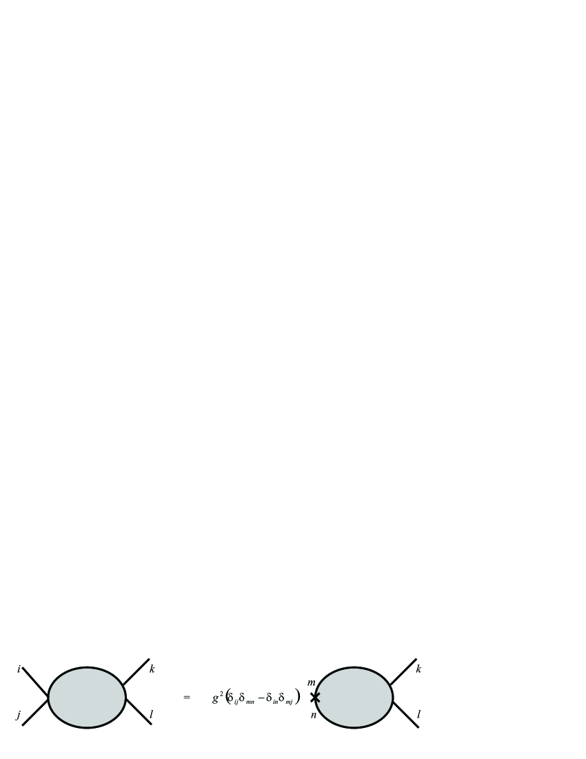
Figure 5: A diagrammatical identity.

Because of the diagrammatical identity shown in FIG.5, with ${}^{m}\textrm{---x---}^{n}$ a $\overline{\psi}_{m}\psi_{n}$ insertion, we have a relation between the $2PPR$ part of coupling constant and mass renormalization.

$$\delta Z_{4;ij,kl}^{2PPR}=\left(\delta_{ij}\delta_{mn}-\delta_{in}\delta_{mj}\right)\delta Z_{2;mn,kl}$$ (14)

This identity can be used to show that the divergent effective mass $\overline{m}$, given by (6), gets replaced by a finite renormalized mass $\overline{m}_{R}=Z_{2}\overline{m}=-g^{2}\left(1-\frac{1}{2N}\right)\Delta_{R}$, where $\Delta_{R}=Z_{2}\Delta$ is the finite, renormalized expectation value of the composite operator $\overline{\psi}\psi$. Indeed, let us consider a generic $2PPR$ subgraph or bubble graph with a $2PPR$ vertex $x$. The divergent subgraphs of this bubble graph, which do not contain $x$, can be made finite by the usual counterterms for wavefunction and coupling constant renormalization. The resulting effective mass will be given by (6), but now with $\Delta=\left\langle\overline{\psi}{\psi}\right\rangle$ evaluated with the full Lagrangian, i.e. including counterterms. We still have to consider the subgraphs of the bubble graph which do contain the $2PPR$ vertex $x$. They can be made finite by coupling constant renormalization, but because the subgraph is $2PPR$ at $x$, only the $2PPR$ part of the counterterm has to be inserted and we get the contribution (see FIG.6)

$$-g^{2}\delta Z_{4;ij,kl}^{2PPR}\Delta_{kl}=-g^{2}\left(\delta_{ij}\delta Z_{2;mm,kk}-\delta Z_{2;ij,kk}\right)\frac{\Delta}{2N}$$ (15)

where use was made of (3) and (14).

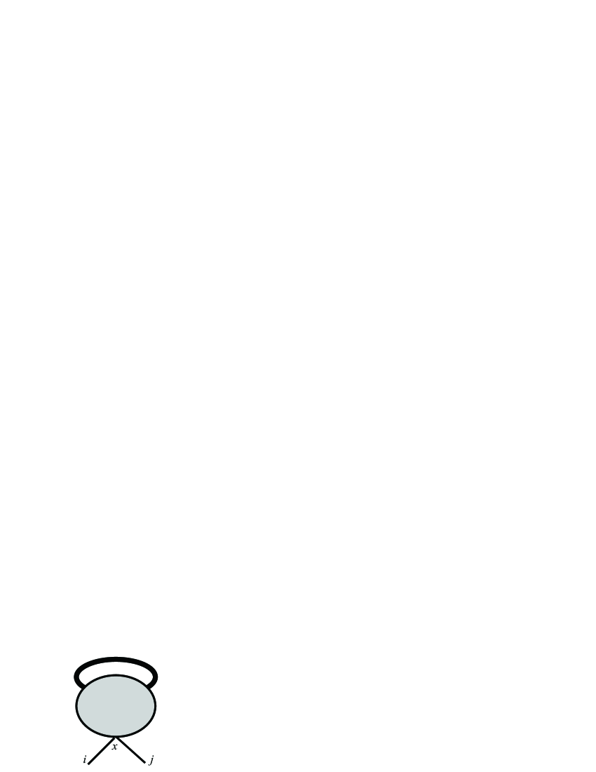
Figure 6: Divergent subgraph containing the $2PPR$ vertex $x$. Fat lines denote full propagators.

Since for a diagonal mass matrix, we can define $\delta Z_{2}$ by

$$\delta Z_{2}\delta_{kl}=\delta Z_{2;mm,kl}$$ (16)

we have

$$2N\delta Z_{2}=\delta Z_{2;mm,kk}$$ (17)

and

$$\delta Z_{2;ij,kk}=\delta Z_{2}\delta_{ij}$$ (18)

After substition of (17) and (18) into (15), we find that the contribution of the $2PPR$ counterterm insertion gives

$$-\delta_{ij}g^{2}\left(1-\frac{1}{2N}\right)\delta Z_{2}\Delta$$ (19)

and hence a mass renormalization

$$\delta\overline{m}=-g^{2}\left(1-\frac{1}{2N}\right)\delta Z_{2}\Delta$$ (20)

so that we obtain a finite, effective renormalized mass

$$\overline{m}_{R}=Z_{2}\overline{m}=-g^{2}\left(1-\frac{1}{2N}\right)\Delta_{R}$$ (21)

with $\Delta_{R}=Z_{2}\Delta=Z_{2}\left\langle\overline{\psi}\psi\right\rangle$ the finite, renormalized VEV of the composite operator $\overline{\psi}\psi$.

To obtain a finite, renormalized expression for the vacuum energy as a function of $\Delta_{R}$ or $\overline{m}_{R}$, we have to use the same trick as in the unrenormalized case and consider the renormalization of $\frac{dE}{dg^{2}}$. Let us first consider the case when the vertex $x$ hit by $\frac{d}{dg^{2}}$ is a $2PPR$ vertex and restrict ourselves to divergent subgraphs which contain $x$ (the ones not containing $x$ pose no problem and simply replace the original $\Delta$ evaluated without counterterms by $\Delta$ with counterterms included). The divergent subgraph can just end at $x$ from the left or the right (FIG.7$a$ and 7$b$) or the $2PPR$ vertex $x$ can be embedded in it (FIG.7$c$).

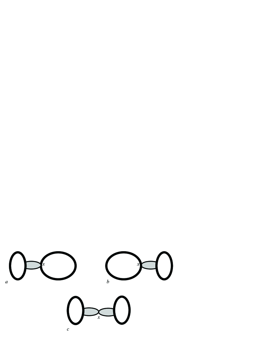
Figure 7: Divergent subgraphs of $\frac{dE}{dg^{2}}$ containing the $2PPR$ vertex $x$.

Graphs 7$a$ en 7$b$ can be made finite by the $2PPR$ part of the coupling constant counterterm and making use of (14), their renormalization contributes

$$(7a)+(7b) = 2\left(-\frac{1}{2}\right)\Delta_{kl}\delta Z_{2;ij,kl}\left(\delta_{ij}\delta_{pq}-\delta_{iq}\delta_{pj}\right)\Delta_{pq}$$ (22)

$$= -\left(1-\frac{1}{2N}\right)\delta Z_{2}\Delta^{2}$$

where we have used (3), (14) and (17). Graph 7$c$ can be made finite with that part of coupling constant renormalization that factorizes at the $2PPR$ vertex $x$. Its renormalization therefore contributes

$$(7c) = -\frac{1}{2}\Delta_{kl}\left(\delta Z_{2;ii,kl}\delta Z_{2;jj,pq}-\delta Z_{2;ij,kl}\delta Z_{2;ij,pq}\right)\Delta_{pq}$$ (23)

$$= -\frac{1}{2}\left(1-\frac{1}{2N}\right)\delta Z_{2}^{2}\Delta^{2}$$

where we made use of (17) and (18). Adding the counterterm contributions (22) and (23) to the original unrenormalized expression (4), we obtain $-\frac{1}{2}\left(1-\frac{1}{2N}\right)\left(Z_{2}\Delta\right)^{2}=-\frac{1}{2}\left(1-\frac{1}{2N}\right)\Delta_{R}^{2}$, which is finite. When $\frac{d}{dg^{2}}$ hits a $2PPI$ vertex, we can unambiguously subdivide the vacuum diagrams in a maximal $2PPI$ part, which contains the vertex hit by $\frac{d}{dg^{2}}$, and one or more $2PPR$ bubble insertions which, after renormalization, can be replaced by the effective renormalized mass $\overline{m}_{R}$. We therefore have

$$\frac{dE}{dg^{2}}=-\frac{1}{2}\left(1-\frac{1}{2N}\right)\Delta_{R}^{2}+\frac{\partial E_{2PPI}}{\partial g^{2}}\left(\overline{m}_{R},g^{2}\right)$$ (24)

We still have to show that the usual counterterms make $\frac{\partial E_{2PPI}}{\partial g^{2}}\left(\overline{m}_{R},g^{2}\right)$ finite. The non-perturbative mass $\overline{m}_{R}$, running in the propagatorlines, will now generate selfenergies which require mass renormalization, which is not present in the original Lagrangian. Again coupling constant renormalization will solve the problem. Let us consider a generic selfenergy subgraph which needs mass renormalization. Since the divergence is linear in $\overline{m}_{R}$, we can restrict ourselves to $2PPI$ diagrams with only one $2PPR$ bubble insertion (FIG.8).

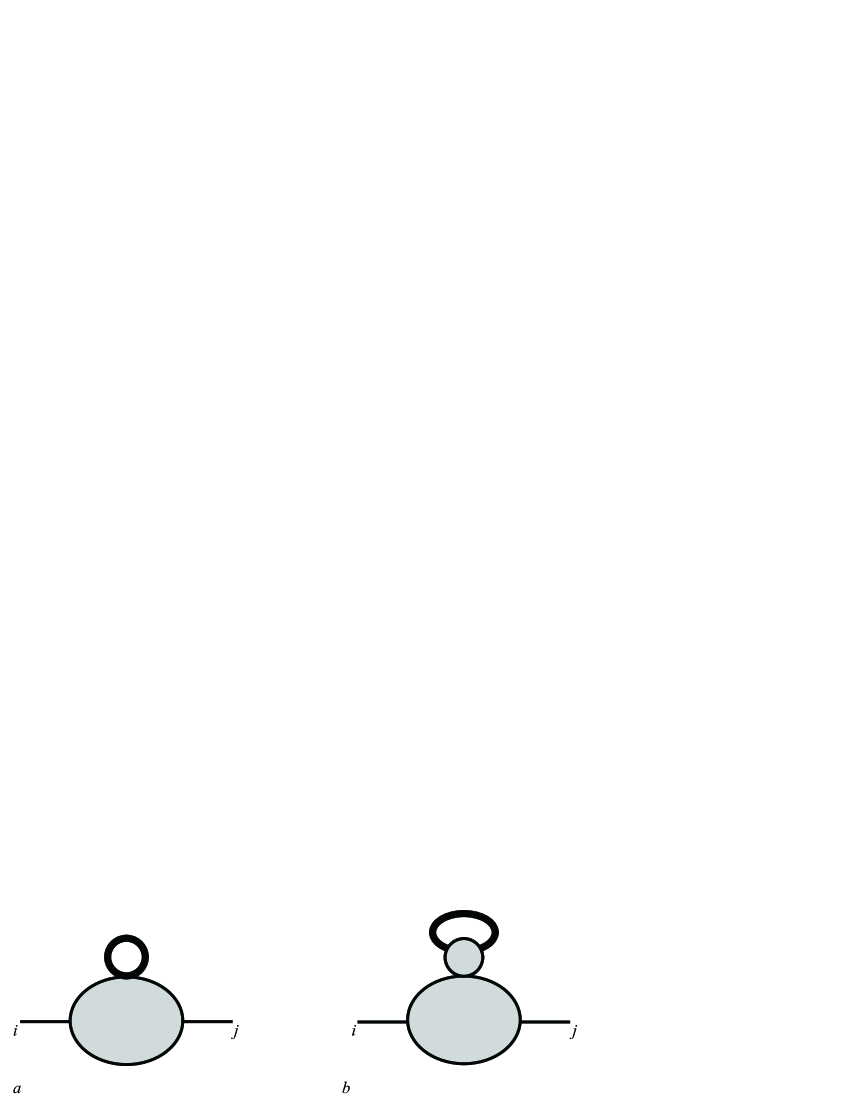
Figure 8: Selfenergy subgraphs needing mass renormalization.

The divergent part of this subgraph, that one wants to renormalize, can end at the $2PPR$ vertex (FIG.8$a$) or can continue throughout the $2PPR$ bubble (FIG.8$b$). In the first case, one needs the $2PPR$ part of coupling constant renormalization which contains only one $2PPR$ vertex (because the divergent part considered belongs to the $2PPI$ part of the diagram). We obviously have

$$\delta Z_{4;ij,kl}^{2PPR,1}=\left(\delta_{ij}\delta_{mn}-\delta_{in}\delta_{mj}\right)\delta Z_{2;mn,kl}^{2PPI}$$ (25)

so that the counterterm contribution is

$$(8a) = -g^{2}\Delta_{kl}\delta Z_{4;kl,ij}^{2PPR,1}$$ (26)

$$= -g^{2}\Delta\left(1-\frac{1}{2N}\right)\delta Z_{2}^{2PPI}\delta_{ij}$$

where use was made of (16) and (25).
In the second case, the divergence factorizes into a $2PPR$ coupling constant renormalization part (the bubble graph part) and a $2PPI$ mass renormalization part, so that the counterterm contribution is

$$(8b) = -g^{2}\Delta_{kl}\delta Z_{4;mn,kl}^{2PPR}\delta Z_{2;mn,ij}^{2PPI}$$ (27)

$$= -g^{2}\Delta\left(1-\frac{1}{2N}\right)\delta Z_{2}\delta Z_{2}^{2PPI}\delta_{ij}$$

Adding both contributions, the relevant parts of the coupling constant counterterms give

$$(8a)+(8b) = -g^{2}Z_{2}\Delta\left(1-\frac{1}{2N}\right)\delta Z_{2}^{2PPI}\delta_{ij}$$ (28)

$$= \overline{m}_{R}\delta Z_{2}^{2PPI}\delta_{ij}$$

which is exactly what we need for mass renormalization in $E_{2PPI}$.

In an analoguous way, we can consider the logarithmic overall divergences of the vacuum diagrams which are quadratic in $\overline{m}_{R}$. We now consider $2PPI$ vacuum diagrams with two bubble insertions. One type of coupling constant renormalization subgraphs end at both $2PPR$ vertices (FIG.9).

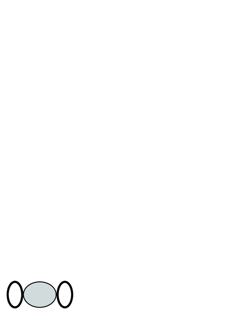
Figure 9: Coupling constant renormalization graph with 2 $2PPR$ vertices.

They can be renormalized by the corresponding $2PPR$ part of the coupling constant renormalization counterterm.

$$\delta Z_{4;ij,kl}^{2PPR,2}=g^{2}\left(\delta_{ij}\delta_{mn}-\delta_{in}\delta_{mj}\right)\delta\zeta_{mn,rs}^{2PPI}\left(\delta_{rs}\delta_{kl}-\delta_{rl}\delta_{ks}\right)$$ (29)

where $\delta\zeta_{mn,rs}$ is the overal divergent part of $\left\langle\overline{\psi}_{m}\psi_{n}\overline{\psi}_{r}\psi_{s}\right\rangle$. Adding the contributions from coupling constant renormalization graphs which also go through the bubble parts, we find

$$\delta E_{2PPI}=\frac{1}{2}\delta Z_{4;ij,kl}^{2PPR,2}\Delta_{ij}^{R}\Delta_{kl}^{R}=\frac{1}{2}\overline{m}_{R}^{2}\delta\zeta^{2PPI}$$ (30)

with

$$\delta\zeta^{2PPI}=\delta\zeta_{mm,nn}^{2PPI}$$ (31)

and use was made of (29).
Again coupling constant renormalization provides us with the necessary additive renormalization of the $2PPI$ vacuum energy. Furthermore, completely analogous arguments can be used to show that the unrenormalized gap equation (10) gets renormalized to

$$\frac{\partial E_{2PPI}}{\partial\overline{m}_{R}}\left(\overline{m}_{R},g\right)=\Delta_{R}$$ (32)

It is clear that the $2PPI$ coupling constant and wave function renormalization subgraphs can be renormalized with the original counterterms. We therefore conclude that $\frac{\partial E_{2PPI}}{\partial g^{2}}\left(\overline{m}_{R},g\right)$ is finite and hence (24) is finite and can be integrated. Making use of the gap equation (32), we find

$$E\left(g^{2}\right)=\frac{1}{2}g^{2}\left(1-\frac{1}{2N}\right)\Delta_{R}^{2}+E_{2PPI}\left(\overline{m}_{R},g^{2}\right)$$ (33)

Of course, we also have the equivalence (12) in the renormalized case.

For the rest of the paper, it is implicitly understood we’re working with renormalized quantities, so that we can drop the $R$-subscripts.

IV Preliminary results for the mass gap and vacuum energy

FIG.10 shows the first terms in the loop expansion for $E_{2PPI}$.

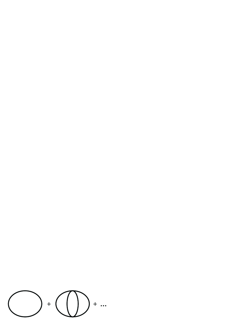
Figure 10: $E_{2PPI}$.

Restricting ourselves to the 1 loop vacuum bubble, we have in dimensional regularization with $d=2-\varepsilon$,

$$E_{2PPI}=-2N\overline{m}^{2}\frac{1}{2-\varepsilon}\mu^{\varepsilon}\int\frac{d^{d}p}{(2\pi)^{d}}\frac{1}{p^{2}+\overline{m}^{2}}$$ (34)

Using the $\overline{MS}$ scheme, we arrive at

$$E=\frac{1}{2}g^{2}\left(1-\frac{1}{2N}\right)\Delta^{2}+\frac{N}{4\pi}\overline{m}^{2}\left(\ln\frac{{\overline{m}}^{2}}{\overline{\mu}^{2}}-1\right)$$ (35)

The gap equation (32) gives

$$\frac{N\overline{m}}{2\pi}\ln\frac{\overline{m}^{2}}{\overline{\mu}^{2}}=\overline{\Delta}$$ (36)

Consequently, the vacuum energy is expressed by

$$E=-\frac{N}{4\pi}\overline{m}^{2}$$ (37)

At 1 loop order, we have

$$\overline{g}^{2}(\overline{\mu})=\frac{1}{\beta_{0}\ln\frac{\overline{\mu}^{2}}{\Lambda_{\overline{MS}}^{2}}}$$ (38)

where $\beta_{0}$ is the leading order coefficient of the $\overline{\beta}$-function

$$\overline{\mu}\frac{\partial\overline{g}^{2}}{\partial\overline{\mu}}=\overline{\beta}(\overline{g}^{2})=-2\left(\beta_{0}\overline{g}^{4}+\beta_{1}\overline{g}^{6}+\overline{\beta}_{2}\overline{g}^{8}+\cdots\right)$$ (39)

The values of the coefficients can be found in Gracey1 ; Gracey2 ; Gracey3 ; Luperini

$$\beta_{0} = \frac{N-1}{2\pi}$$ (40)

$$\beta_{1} = -\frac{N-1}{4\pi^{2}}$$ (41)

$$\overline{\beta}_{2} = -\frac{(N-1)\left(N-\frac{7}{2}\right)}{16\pi^{3}}$$ (42)

To get a numerical value for the mass gap , we have to choose the subtraction scale $\overline{\mu}$. The choice immediately coming to mind is setting $\overline{\mu}=\overline{m}$, which eliminates the potentially large logarithm present in (35). Doing so, we find, next to the perturbative solution $\overline{m}=0$,

$$m=\overline{m}=\Lambda_{\overline{MS}}$$ (43)

while

$$E=-\frac{N}{4\pi}\Lambda_{\overline{MS}}^{2}$$ (44)

The exact mass gap is given by Forgacs

$$m_{exact}=(4e)^{\frac{1}{2N-2}}\frac{1}{\Gamma\left(1-\frac{1}{2N-2}\right)}\Lambda_{\overline{MS}}$$ (45)

while the exact vacuum energy is Zamo

$$E_{exact}=-\frac{1}{8}m_{exact}^{2}\cot\left(\frac{\pi}{2(N-1)}\right)$$ (46)

We expect that the error on $E$ consists of the error on the mass squared and the error on the function multiplying that mass squared. Therefore we will consider the quantity $\sqrt{-E}$ to test the reliability of our results. We define the deviations in terms of percentage $P$ and $Q$, i.e.

$$P = 100\frac{m_{eff}-m_{exact}}{m_{exact}}$$ (47)

$$Q = 100\frac{\sqrt{-E}-\sqrt{-E_{exact}}}{\sqrt{-E_{exact}}}$$ (48)

Looking at TABLE 1, we notice that our results are quite acceptable.

Table 1: 1 loop results for mass gap and vacuum energy

$N$	$P$	$Q$	$P_{1/N}$	$Q_{1/N}$
2	-46.3%	-	-21.9%	-
3	-32.5%	-6.7%	-12.2%	5.8%
4	-24.2%	-8.0%	-7.0%	1.3%
5	-19.1%	-7.2%	-4.5%	0.4%
6	-15.8%	-6.2%	-3.1%	0.1%
7	-13.5%	-5.5%	-2.3%	0.007%
8	-11.7%	-4.8%	-1.8%	-0.03%
9	-10.4%	-4.3%	-1.4%	-0.04%
10	-9.3%	-3.9%	-1.1%	-0.04%
20	-4.6%	-2.0%	-0.3%	-0.02%

We notice there is convergence ($P\rightarrow 0$ and $Q\rightarrow 0$) to the exact result in case of $N\rightarrow\infty$. In fact, we recovered the $N\rightarrow\infty$ approximation. For comparison, we also displayed the next to leading results , given by expanding (45) and (46) in powers of $1/N$.

$$m_{1/N} = \left(1+\frac{1-\gamma_{E}+\ln 4}{2N}+\mathcal{O}\left(\frac{1}{N^{2}}\right)\right)\Lambda_{\overline{MS}}$$ (49)

$$E_{1/N} = \left(-\frac{N}{4\pi}+\frac{\gamma_{E}-\ln 4}{4\pi}+\mathcal{O}\left(\frac{1}{N}\right)\right)\Lambda_{\overline{MS}}^{2}$$ (50)

where $\gamma_{E}\approx 0.577216$ is the Euler-Mascheroni constant.
However, the choice $\overline{\mu}=\overline{m}=\Lambda_{\overline{MS}}$ cannot satisfy us, since we are expanding in $\overline{g}^{2}(\overline{m})=\infty$. We may have qualitatively good results, but for a field theory where the exact results are unknown, $\overline{g}^{2}=\infty$ gives by no means an indication about how trustworthy our approximations are. It is clear we must find a better method to achieve results with the $2PPI$ expansion.

V Optimization and 2 loop corrections

V.1 Renormalization group equation for $E$

A standard approach to get better results is the usage of the renormalization group equation (RGE). In our approach, we first solved the gap equation and then set $\overline{\mu}=\overline{m}$. Normally, when minimizing the effective potential $V$, one first sets $\overline{\mu}=\overline{m}$, and afterwards the RGE is used to sum leading logarithms, while all quantities are running according to their renormalization group equations at scale $\overline{m}$. We already mentioned $E$ cannot be treated on equal footing with an effective potential due to the demand that $\frac{\partial E}{\partial\overline{m}}=0$ must hold. We first point out why this also disturbs a standard RGE improvement of $E$.

Since $E$ is the vacuum energy, it is a physical quantity and therefore, it shouldn’t depend on the subtraction scale $\overline{\mu}$. This is expressed in a formal way by means of the RGE

$$\overline{\mu}\frac{dE}{d\overline{\mu}}=0$$ (51)

In a perturbative series expansion, this means the differential equation (51) must be fulfilled order by order, when all quantities obey their running w.r.t. $\overline{\mu}$. Out of (16), we extract the running of $\overline{m}$, namely

$$\overline{\mu}\frac{\partial\overline{m}}{\partial\overline{\mu}}=\left(\frac{\overline{\beta}(\overline{g}^{2})}{\overline{g}^{2}}+\overline{\gamma}(\overline{g}^{2})\right)\overline{m}\equiv\overline{\kappa}(\overline{g}^{2})\overline{m}$$ (52)

where $\overline{\gamma}(\overline{g}^{2})$ governs the scaling behaviour of $\overline{\Delta}$

$$\overline{\mu}\frac{\partial\overline{\Delta}}{\partial\overline{\mu}}=\overline{\gamma}(\overline{g}^{2})\overline{\Delta}$$ (53)

with

$$\overline{\gamma}(\overline{g}^{2})=\gamma_{0}\overline{g}^{2}+\overline{\gamma}_{1}\overline{g}^{4}+\overline{\gamma}_{2}\overline{g}^{6}+\cdots$$ (54)

The coefficients are given by Gracey1 ; Gracey2 ; Gracey3 ; Luperini

$$\gamma_{0} = \frac{N-\frac{1}{2}}{\pi}$$ (55)

$$\overline{\gamma}_{1} = -\frac{N-\frac{1}{2}}{4\pi^{2}}$$ (56)

$$\overline{\gamma}_{2} = -\frac{\left(N-\frac{1}{2}\right)\left(N-\frac{3}{4}\right)}{4\pi^{3}}$$ (57)

After some calculation, we find

$$\overline{\mu}\frac{dE}{d\overline{\mu}} = \left(\overline{\mu}\frac{\partial}{\partial\overline{\mu}}+\overline{\beta}(\overline{g}^{2})\frac{\partial}{\partial\overline{g}^{2}}+\overline{\kappa}(\overline{g}^{2})\overline{m}\frac{\partial}{\partial\overline{m}}\right)E$$ (58)

$$= \frac{1}{4\pi}\frac{\overline{m}^{2}}{1-\frac{1}{2N}}+\mathcal{O}(\overline{g}^{2})$$

It seems that $E$ doesn’t obey its RGE. Perturbatively, it of course fullfills the RGE up to $\mathcal{O}\left(g^{2}\right)$ since $\overline{m}=0$ to all orders in perturbation theory. We must not be tempted to interpret this failure as the need to introduce some non-perturbative running coupling constant, as can be found in literature sometimes. The nature of the apparent problem lies in the fact that we forgot about the gap equation $\frac{\partial E}{\partial\overline{m}}=0$, because only then our $2PPI$ expression for $E$ is meaningful. (36) gives that

$$\ln\frac{\overline{m}^{2}}{\overline{\mu}^{2}}\propto\frac{1}{\overline{g}^{2}}$$ (59)

It is easy to check that (59) means that all leading log terms in the expansion of $E$ are of the order unity. Consequently, we cannot simply show order by order that $\overline{\mu}\frac{dE}{d\overline{\mu}}=0$.
The problem extends to higher orders: when we would calculate $E$ up to a certain order $n$, we would need knowledge of all leading, subleading,…, $n^{th}$ leading log terms.
The above discussion reveals a possible strategy : we could do a (leading) log expansion for $E_{2PPI}$, with a source $J$ coupled to $\overline{\psi}\psi$. Then we could use the RGE for $E$ to sum all (leading) logs in $E_{2PPI}$. We leave this idea, because the RGE for $E$ itself is non-linear when $J\neq 0$ . This is accompanied with its own problems. A thorough discussion of this subject can be consulted in Verschelde3 .

We conclude that we cannot use the RGE for $E$ to optimize that what we did hitherto. The crucial point is that the gap equation must hold for consistency. We can only set $\overline{\mu}=\overline{m}$ in $\frac{\partial E}{\partial\overline{m}}$ after deriving $E$ w.r.t. $\overline{m}$ and solving this gap equation, not before.

V.2 Optimization

We have seen that the $\overline{MS}$ scheme is not optimal for the $2PPI$ expansion used on GN. We could have renormalized the coupling constant in another way and hope that this gives better results. It is easily verified that going to a scheme with coupling $g^{2}$, determined at lowest order by $\overline{g}^{2}=g^{2}\left(1+b_{0}g^{2}\right)$, gives the same results as in (43) and (44), but now with $g^{2}=b_{0}^{-1}$. This means results are as good as before, but for a sufficiently large $b_{0}$, $g^{2}$ is small. Again, we put $\overline{\mu}=\overline{m}$ to cancel logarithms.
Till now, we kept $\overline{m}$ as the mass parameter, however we should go to another scheme for this quantity too. The results are then no longer independent of the renormalization prescriptions, i.e. if $\overline{m}=m\left(1+a_{0}g^{2}\right)$ at lowest order, then $a_{0}$ enters the final results, and $a_{0}$ is completely free to choose. We tackle the problem of freedom of renormalization of the coupling constant and mass parameter in 4 consecutive steps.


Step 1
First of all, we remove the freedom how the mass parameter is renormalized. We can replace $\overline{m}$ by an unique $M$ such that $M$ is renormalization scale and scheme independent (RSSI) Karel . Out of (52), we immediately deduce that

$$M=\overline{f}(\overline{g}^{2})\overline{m}$$ (60)

where $\overline{f}(\overline{g}^{2})$ is the solution of

$$\overline{\mu}\frac{\partial\overline{f}}{\partial\overline{\mu}}=-\overline{\kappa}(\overline{g}^{2})\overline{f}$$ (61)

When we change our MRS, we have relations of the form

$$\overline{g}^{2} = g^{2}\left(1+b_{0}g^{2}+b_{1}g^{4}+\cdots\right)$$ (62)

$$\overline{m} = m\left(1+m_{0}g^{2}+m_{1}g^{4}+\cdots\right)$$ (63)

$$\overline{f}(\overline{g}^{2}) = f(g^{2})\left(1+f_{0}g^{2}+f_{1}g^{4}+\cdots\right)$$ (64)

Whenever a quantity is barred, it’s understood we’re considering $\overline{MS}$, otherwise we’re considering an arbitrary MRS . Using the foregoing relations, it is easy to show the scheme independence of $M$.

The explicit solution, up to the order we will need it, is given by

$$\overline{f}(\overline{g}^{2}) = (\overline{g}^{2})^{-1+\frac{\gamma_{0}}{2\beta_{0}}}\left\{1\vphantom{\frac{\gamma_{0}\left(\frac{\beta_{1}^{2}}{\beta_{0}^{2}}-\frac{\overline{\beta}_{2}}{\beta_{0}}\right)}{\beta_{0}}}+\frac{\overline{g}^{2}}{2}\left(-\frac{\beta_{1}\gamma_{0}}{\beta_{0}^{2}}+\frac{\overline{\gamma}_{1}}{\beta_{0}}\right)\right.$$ (65)

$$+ \left.\frac{\overline{g}^{4}}{4}\left[\vphantom{\frac{\gamma_{0}\left(\frac{\beta_{1}^{2}}{\beta_{0}^{2}}-\frac{\overline{\beta}_{2}}{\beta_{0}}\right)}{\beta_{0}}}\frac{1}{2}\left(-\frac{\beta_{1}\gamma_{0}}{\beta_{0}^{2}}+\frac{\overline{\gamma}_{1}}{\beta_{0}}\right)^{2}\right.\right.$$

$$+ \left.\left.\frac{\gamma_{0}\left(\frac{\beta_{1}^{2}}{\beta_{0}^{2}}-\frac{\overline{\beta}_{2}}{\beta_{0}}\right)}{\beta_{0}}-\frac{\beta_{1}\overline{\gamma}_{1}}{\beta_{0}^{2}}+\frac{\overline{\gamma}_{2}}{\beta_{0}}\right]\right\}$$

Next, we rewrite $\overline{m}$ in terms of $M$ by inverting (60)

$$\overline{m}=M(\overline{g}^{2})^{1-\frac{\gamma_{0}}{2\beta_{0}}}\left(1+c_{1}\overline{g}^{2}+c_{2}\overline{g}^{4}\right)$$ (66)

where

$$c_{1} = \frac{1}{2}\left(\frac{\beta_{1}\gamma_{0}}{\beta_{0}^{2}}-\frac{\overline{\gamma}_{1}}{\beta_{0}}\right)$$ (67)

$$c_{2} = \frac{1}{8}\left(-\frac{\beta_{1}\gamma_{0}}{\beta_{0}^{2}}+\frac{\overline{\gamma}_{1}}{\beta_{0}}\right)^{2}-\frac{1}{4}\left(\frac{\gamma_{0}\left(\frac{\beta_{1}^{2}}{\beta_{0}^{2}}-\frac{\overline{\beta}_{2}}{\beta_{0}}\right)}{\beta_{0}}\right)$$ (68)

$$+ \frac{1}{4}\left(\frac{\beta_{1}\overline{\gamma}_{1}}{\beta_{0}^{2}}-\frac{\overline{\gamma}_{2}}{\beta_{0}}\right)$$

Step 2
Transformation (66) allows to rewrite $E$ in terms of $M$. Since the next contribution to (35) is proportional to $\overline{g}^{4}\overline{m}^{2}$ (see FIG.10), we can rewrite $E$ up to order $\overline{g}^{2}$ when (66) is applied. Explicitly,

$$E = M^{2}(\overline{g}^{2})^{2-\frac{\gamma_{0}}{\beta_{0}}}\left[\vphantom{\frac{1}{2\left(1-\frac{1}{2N}\right)}\left(\frac{1}{\overline{g}^{2}}\right)}\frac{N}{4\pi}\left(1+2c_{1}\overline{g}^{2}\right)\right.$$ (69)

$$\times \left.\left(\ln\frac{M^{2}}{\overline{\mu}^{2}}+\left(2-\frac{\gamma_{0}}{\beta_{0}}\right)\ln\overline{g}^{2}\right)-\frac{N}{4\pi}\right.$$

$$+ \left.\frac{1}{2\left(1-\frac{1}{2N}\right)}\left(\frac{1}{\overline{g}^{2}}+2c_{1}+\left(2c_{2}+c_{1}^{2}\right)\overline{g}^{2}\right)\right]$$

It is important to notice that the demand $\frac{\partial E}{\partial\overline{m}}=0$ is translated into $\frac{\partial E}{\partial M}=0$, because $M$ and $\overline{m}$ differ only by an overall factor $\overline{f}$ which depends solely on $\overline{g}^{2}(\overline{\mu})$.

Step 3
(69) is still written in terms of $\overline{g}^{2}$. Using (62), we exchange $\overline{g}^{2}$ for $g^{2}$, where the $b_{i}$ parametrize the coupling constant renormalization. We find

$$E = M^{2}(g^{2})^{2-\frac{\gamma_{0}}{\beta_{0}}}\left(\frac{e_{-1}}{g^{2}}+e_{0}+e_{1}g^{2}\right)$$ (70)

with

$$e_{-1} = \frac{1}{2\left(1-\frac{1}{2N}\right)}$$ (71)

$$e_{0} = -\frac{N}{4\pi}+\frac{-b_{0}+2c_{1}}{2\left(1-\frac{1}{2N}\right)}+\frac{b_{0}U}{2\left(1-\frac{1}{2N}\right)}+\frac{N}{4\pi}V$$ (72)

$$e_{1} = \frac{b_{0}^{2}-b_{1}+c_{1}^{2}+2c_{2}}{2\left(1-\frac{1}{2N}\right)}$$ (73)

$$+ \frac{1}{2\left(1-\frac{1}{2N}\right)}\left(b_{1}U+\frac{b_{0}^{2}}{2}U(U-1)\right)$$

$$+ b_{0}U\left(-\frac{N}{4\pi}+\frac{-b_{0}+2c_{1}}{2\left(1-\frac{1}{2N}\right)}+\frac{N}{4\pi}V\right)$$

$$+ \frac{N}{4\pi}\left(b_{0}U+2c_{1}V\right)$$

$$U = 2-\frac{\gamma_{0}}{\beta_{0}}$$ (74)

$$V = \ln{\frac{M^{2}}{\overline{\mu}^{2}}}+\left(2-\frac{\gamma_{0}}{\beta_{0}}\right)\ln g^{2}$$ (75)

Step 4
Consider (70). We notice that the degrees of freedom, concerning the scheme, are settled in the $b_{i}$. When we rewrite the expansion in terms of $g^{2}_{1loop}$ instead of $g^{2}$, all scheme dependence is reduced to one parameter, namely $b_{0}$. This was also recognized in Karel . It is in a way more ”natural” to rewrite a perturbative series in terms of $g^{2}_{1loop}$, because $g^{2}$ itself is changed whenever we include the next loop order, while $g^{2}_{1loop}$ of course remains the same.
The necessary formulas are given by

$${g}^{2}(\overline{\mu}) = \frac{1}{x}-\frac{\beta_{1}}{\beta_{0}}\frac{\ln\frac{x}{\beta_{0}}}{x^{2}}$$ (76)

$$+ \frac{\left(\frac{\beta_{1}}{\beta_{0}}\right)^{2}\left(\left(\ln\frac{x}{\beta_{0}}\right)^{2}-\ln\frac{x}{\beta_{0}}\right)+\left(\frac{\beta_{2}}{\beta_{0}}-\left(\frac{\beta_{1}}{\beta_{0}}\right)^{2}\right)}{x^{3}}$$

$$+ \mathcal{O}\left(\frac{1}{x^{4}}\right)$$

where

$$x=\frac{1}{g^{2}_{1loop}}=\beta_{0}\ln\frac{\overline{\mu}^{2}}{\Lambda^{2}}$$ (77)

$\Lambda$ is the scale parameter of the corresponding MRS. In Celmaster , it was shown that

$$\Lambda=\Lambda_{\overline{MS}}e^{-\frac{b_{0}}{2\beta_{0}}}$$ (78)

For $\beta_{2}$, we have Grunberg

$$\beta_{2}=(b_{0}^{2}-b_{1})\beta_{0}+\beta_{1}b_{0}+\overline{\beta}_{2}$$ (79)

Since (70) is correct up to order $g^{2}M^{2}$, we can expand up to order $x^{-1}M^{2}$. Using (76), (78) and (79), the vacuum energy becomes

$$E = M^{2}\left(\frac{1}{x}\right)^{2-\frac{\gamma_{0}}{\beta_{0}}}\left(E_{-1}x+E_{0}+\frac{E_{1}}{x}\right)$$ (80)

with

$$E_{-1} = \frac{1}{2\left(1-\frac{1}{2N}\right)}$$ (81)

$$E_{0} = -\frac{N}{4\pi}+\frac{-b_{0}+2c_{1}}{2\left(1-\frac{1}{2N}\right)}+\frac{b_{0}U}{2\left(1-\frac{1}{2N}\right)}$$ (82)

$$- \frac{\beta_{1}(U-1)L}{2\beta_{0}\left(1-\frac{1}{2N}\right)}+\frac{N}{4\pi}W$$

$$E_{1} = \frac{c_{1}^{2}+2c_{2}}{2\left(1-\frac{1}{2N}\right)}+\frac{\frac{\beta_{1}^{2}}{\beta_{0}^{2}}(1+L)-\frac{b_{0}\beta_{1}+\overline{\beta}_{2}}{\beta_{0}}}{2\left(1-\frac{1}{2N}\right)}$$ (83)

$$- \frac{N}{4\pi}\frac{\beta_{1}}{\beta_{0}}UL+\frac{b_{0}^{2}U(U-1)}{4\left(1-\frac{1}{2N}\right)}+\frac{1}{2\left(1-\frac{1}{2N}\right)}$$

$$\times \left[\left(-\frac{\beta_{1}^{2}}{\beta_{0}^{2}}\left(1+L-L^{2}\right)+\frac{b_{0}^{2}\beta_{0}+b_{0}\beta_{1}+\overline{\beta}_{2}}{\beta_{0}}\right)U\right.$$

$$+ \left.\frac{\beta_{1}^{2}L^{2}U(U-1)}{2\beta_{0}^{2}}\right]+b_{0}U\left[\vphantom{\frac{2c_{1}-b_{0}}{2\left(1-\frac{1}{2N}\right)}}\frac{N}{4\pi}(W-1)\right.$$

$$+ \left.\frac{2c_{1}-b_{0}}{2\left(1-\frac{1}{2N}\right)}\right]-\frac{\beta_{1}}{\beta_{0}}LU\left[\vphantom{\frac{2c_{1}-b_{0}}{2\left(1-\frac{1}{2N}\right)}}\frac{N}{4\pi}(W-1)\right.$$

$$+ \left.\frac{2c_{1}-b_{0}}{2\left(1-\frac{1}{2N}\right)}+\frac{\beta_{1}L}{2\beta_{0}\left(1-\frac{1}{2N}\right)}+\frac{b_{0}U}{2\left(1-\frac{1}{2N}\right)}\right]$$

$$+ \frac{N}{4\pi}\left(b_{0}U+2c_{1}W\right)$$

$$L = \ln\frac{x}{\beta_{0}}$$ (84)

$$U = 2-\frac{\gamma_{0}}{\beta_{0}}$$ (85)

$$W = \ln{\frac{M^{2}}{\overline{\mu}^{2}}}+\left(2-\frac{\gamma_{0}}{\beta_{0}}\right)\ln\frac{1}{x}$$ (86)

V.3 2 loop corrections

The next order corrections are 2 loop for the mass (the setting sun diagram of FIG.11) and 3 loop for the vacuum energy (the basket ball diagram of FIG.2). We will restrict ourselves to 2 loop corrections. The diagram displayed in FIG.11 gives a mass renormalization. The double line is the full propagator $S_{full}(p)$. We first employ the $\overline{MS}$ scheme again for the calculation.

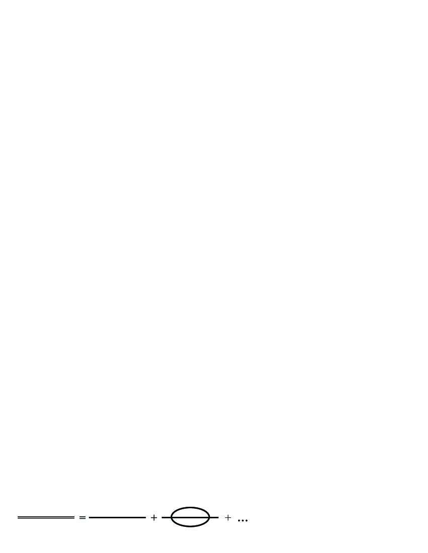
Figure 11: Diagrams needed to calculate $m_{eff}$ in function of $\overline{m}$.

Let $\mathcal{P}$ be the value of the (amputated) setting sun diagram. Since

$$S(p)=\frac{1}{ip/+\overline{m}}$$ (87)

we have

$$S_{2loop}(p)=\frac{1}{ip/+\overline{m}-\mathcal{P}}$$ (88)

The effective mass $m_{eff}$ is the pole of $S_{2loop}$(p). From Verschelde3 , we obtain

$$\mathcal{P} = \left(N-\frac{1}{2}\right)\overline{g}^{4}\left(-\overline{m}I^{2}+ip/\frac{\varepsilon}{2-\varepsilon}I^{2}\right.$$ (89)

$$+ \left.\frac{1}{16\pi^{2}}\left(\overline{m}F_{1}+ip/F_{2}\right)\right)$$

where

$$I = \frac{1}{4\pi}\left[\frac{2}{\varepsilon}-\ln\frac{\overline{m}^{2}}{\overline{\mu}^{2}}\right.$$ (90)

$$+ \left.\frac{\varepsilon}{4}\left(\frac{\pi^{2}}{6}+\ln^{2}\frac{\overline{m}^{2}}{\overline{\mu}^{2}}\right)+\mathcal{O}(\varepsilon^{2})\right]$$

$$F_{1} = -\frac{2\pi^{2}}{9}+12q_{1}-24q_{2}$$ (91)

$$F_{2} = 2-\frac{2\pi^{2}}{3}$$ (92)

$$q_{1} = \int_{0}^{1}dt\frac{\ln t}{t^{2}-t+1}\approx-1.17195$$ (93)

$$q_{2} = \int_{0}^{1}dt\frac{\ln t}{t^{3}+1}\approx-0.951518$$ (94)

Working up to order $\overline{g}^{4}$, we find for the inverse propagator

$$S_{2loop}^{-1}=ip/\left[1-\frac{\left(N-\frac{1}{2}\right)\overline{g}^{4}}{16\pi^{2}}\left(1-2\ln\frac{\overline{m}^{2}}{\overline{\mu}^{2}}+F_{2}\right)\right]$$ (95)

$$+ \overline{m}\left[1+\frac{\left(N-\frac{1}{2}\right)\overline{g}^{4}}{16\pi^{2}}\left(2\ln^{2}\frac{\overline{m}^{2}}{\overline{\mu}^{2}}+\frac{\pi^{2}}{6}-F_{1}\right)\right]$$

Solving for the pole gives

$$m_{eff} = \overline{m}\left[1+\frac{\left(N-\frac{1}{2}\right)\overline{g}^{4}}{16\pi^{2}}\left(2\ln^{2}\frac{\overline{m}^{2}}{\overline{\mu}^{2}}\right.\right.$$ (96)

$$+ \left.\left.\vphantom{\frac{\left(N-\frac{1}{2}\right)\overline{g}^{4}}{16\pi^{2}}}\frac{\pi^{2}}{6}-F_{1}+1-2\ln\frac{\overline{m}^{2}}{\overline{\mu}^{2}}+F_{2}\right)\right]$$

With $\overline{\mu}=\overline{m}=\Lambda_{\overline{MS}}$, the above equation has no sense.

Next, we follow the same steps as executed for $E$ to reexpress $m_{eff}$ in terms of $M$ and $x$. A little algebra results in

$$m_{eff} = M\left(\frac{1}{x}\right)^{1-\frac{\gamma_{0}}{2\beta_{0}}}\left\{1+\frac{1}{x}\left[c_{1}+\frac{b_{0}U}{2}-\frac{\beta_{1}UL}{2\beta_{0}}\right]\right.$$

$$+ \left.\frac{1}{x^{2}}\left[b_{0}c_{1}\left(1+\frac{U}{2}\right)+c_{2}+\frac{U}{2}\times\right.\right.$$

$$\left.\left.\left(\frac{\beta_{1}^{2}}{\beta_{0}^{2}}\left(L^{2}-L-1\right)+\frac{b_{0}^{2}\beta_{0}+b_{0}\beta_{1}+\overline{\beta}_{2}}{\beta_{0}}\right)\right.\right.$$

$$- \left.\left.\frac{b_{0}^{2}\gamma_{0}U}{8\beta_{0}}-\frac{L^{2}\beta_{1}^{2}\gamma_{0}U}{8\beta_{0}^{3}}-\frac{L\beta_{1}\left(1+\frac{U}{2}\right)\left(c_{1}+b_{0}\frac{U}{2}\right)}{\beta_{0}}\right.\right.$$

$$+ \left.\left.\frac{N-\frac{1}{2}}{16\pi^{2}}\left(\frac{\pi^{2}}{6}+1-F_{1}+F_{2}-2W+2W^{2}\right)\right]\right\}$$

The quantities $c_{1}$, $c_{2}$, $U$, $W$ and $L$ are the same as defined before. Again, only $b_{0}$ is left over as scheme parameter.

VI Second numerical results for the mass gap and vacuum energy

We first discuss how we can fix the parameter $b_{0}$ in a reasonable, self-consistent way. A frequently used method is the principle of minimal sensitivity(PMS)Stevenson . This is based on the concept that physical quantities should not depend on the renormalization prescriptions. In our case, the vacuum energy $E$ as well as the mass gap $m_{eff}$ are physical, so we could apply PMS. However, PMS doesn’t always work out. Sometimes there is no minimum, then an alternative is picking that $b_{0}$ for which the derivative of the considered quantity is minimal ($\rightarrow$ as near as possible to a minimum). Also fastest apparent convergence criteria (FACC) can be practiced.

But maybe the biggest barrier to a fruitful use of PMS (or FACC) arises from the same origin why $E$ didn’t seem to obey its RGE. Just as the scale dependence of $E$ is not cancelled order by order, the scheme dependence of $E$ won’t cancel order by order, so we may find no optimal $b_{0}$, and even if we would have such $b_{0}$, it wouldn’t be certain that the corresponding $E$ really is a good approximation to $E_{exact}$. The same obstacle will arise for the mass gap $m_{eff}$.

Apparently, we haven’t got any further. We may have a way out through. $M$, as defined in (60), is RSSI, independent of the fact that it satisfies its gap equation or not. The $2PPI$ formalism provides us with an equation to calculate $M$ approximately. This equation, $\frac{\partial E}{\partial M}=0$, is correct up to a certain order and $M$ is RSSI up to that order by construction. Hence, we can ask that the (non-zero) solution $M$ has minimal dependence on $b_{0}$. This also gives a value for $b_{0}$ to calculate the vacuum energy, because the $b_{0}$ for $E$ and $M$ must be equal, again because $E$ is only correct when the gap equation is fulfilled. Also the mass gap $m_{eff}$ can be calculated with this $b_{0}$.

VI.1 First order results

We start from the expression (80), but we first restrict ourselves to the lowest order correction.

$$E = M^{2}\left(\frac{1}{x}\right)^{2-\frac{\gamma_{0}}{\beta_{0}}}\left(E_{-1}x+E_{0}\right)$$ (98)

Until now, we haven’t said anything about the freedom in scale $\overline{\mu}$. Analogously as we fixed $b_{0}$, we can ask $\frac{\partial M}{\partial\overline{\mu}}=0$ due to the scale independence of $M$. For the sake of simplicity, we will however make a reasonable choice for $\overline{\mu}$. In order to cancel logarithms, we could set $\overline{\mu}=M$. We refer to this as Choice I. We observe that $\ln\frac{M^{2}}{\overline{\mu}^{2}}$ always appears in the form $W\equiv\ln\frac{M^{2}}{\overline{\mu}^{2}}+\left(2-\frac{\gamma_{0}}{\beta_{0}}\right)\ln\frac{1}{x}$; we could determine $\overline{\mu}$ such that $W=0$, then the danger of exploding logarithms is also averted. We refer to this as Choice II.

TABLE 2 and TABLE 3 summarize the corresponding results.

Table 2: Optimized first order results for mass gap and vacuum energy (Choice I)

$N$	$P$	$Q$	$\frac{N}{4\pi x}$
2	?	?	?
3	-22.5%	43.9%	0.60
4	-19.4%	25.9%	0.56
5	-16.8%	17.9%	0.55
6	-14.6%	13.8%	0.54
7	-12.7%	11.3%	0.53
8	-11.2%	9.5%	0.53
9	-10.1%	8.2%	0.53
10	-9.1%	7.2%	0.52
20	-4.5%	3.4%	0.50

Table 3: Optimized first order results for mass gap and vacuum energy (Choice II)

$N$	$P$	$Q$	$\frac{N}{4\pi x}$
2	?	?	?
3	19.9%	120.7%	0.30
4	4.5%	57.2%	0.31
5	0.3%	36.8%	0.32
6	-1.2%	27.0%	0.33
7	-1.9%	21.3%	0.33
8	-2.1%	17.5%	0.34
9	-2.2%	14.9%	0.34
10	-2.2%	12.9%	0.34
20	-1.6%	5.5%	0.35

Some remarks must be made.

1) We have determined the parameter $b_{0}$ by requiring that $\left|\frac{\partial M}{\partial b_{0}}\right|$ is minimal . In FIG.12, $M(b_{0})$ is plotted for the case $N=5$ and Choice I. FIG.13 shows $\frac{\partial M}{\partial b_{0}}$, again for $N=5$ and Choice I. The plots for Choice II are completely similar.
Notice that $\left|\frac{\partial M}{\partial b_{0}}\right|$ is relatively small. For both choices, it tended to zero for growing $N$, f.i. $\left|\frac{\partial M}{\partial b_{0}}\right|\approx 0.045$ for $N=10$, Choice I.

Figure 12: $M(b_{0})$ in units of $\Lambda_{\overline{MS}}$ for $N=5$ (Choice I, 1st order).

Figure 13: $\frac{\partial M}{\partial b_{0}}$ in units of $\Lambda_{\overline{MS}}$ for $N=5$ (Choice I, 1st order).

Results for the mass gap agree very well with the exact values for Choice II, this is quite remarkable since we used a lowest order approximation. Choice I gives almost the same results as the $N\rightarrow\infty$ approximation.

For the vacuum energy, the results are somewhat less good than those obtained with a straightforward $\overline{MS}$ calculation.
Nevertheless, the mass gap as well as the vacuum energy are converging, and we retrieve the correct $N\rightarrow\infty$ limit. Moreover, the relevant expansion parameter $\frac{N}{4\pi x}$ is relatively small, and behaves more or less as a constant.

2) For $N=2$ we didn’t find an optimal $b_{0}$. In the light of the exact results (45) and (46), it isn’t unexpected that $N=2$ causes trouble. $N=2$ is a maximum of $m_{exact}$, and close to $N=\frac{3}{2}$, which is a root of $m_{exact}$. There is a sharp drop between 2 and $\frac{3}{2}$, and somewhat lower than $\frac{3}{2}$, oscillating behaviour begins. What’s more, $N=2$ and $N=\frac{3}{2}$ are both roots of $E_{exact}$, while $E_{exact}>0$ between them. Again there is a sharp drop at $\frac{3}{2}$ with oscillation somewhat before $\frac{3}{2}$. Problems with $N=2$ persist at second order too, as will be seen shortly.

VI.2 Second order results

In TABLE 4, we present second order results for Choice I, while TABLE 5 displays those for Choice II. Just as for the first order approximation, we plotted $M(b_{0})$ in FIG.14, and $\left|\frac{\partial M}{\partial b_{0}}\right|$ in FIG.15 for the case $N=5$, Choice I. Notice that $\left|\frac{\partial M}{\partial b_{0}}\right|$ is smaller at second order. For $N=10$, $\left|\frac{\partial M}{\partial b_{0}}\right|\approx 0.022$ . Again it reaches zero for infinite $N$. Again, we weren’t able to extract a value for $m_{eff}$ or $E$ for $N=2$.

Table 4: Optimized second order results for mass gap and vacuum energy (Choice I)

$N$	$P$	$Q$	$\frac{N}{4\pi x}$
2	?	?	?
3	-0.2%	54.8%	0.16
4	-2.6%	33.5%	0.16
5	-3.3%	23.8%	0.16
6	-3.7%	18.1%	0.16
7	-3.8%	14.5%	0.17
8	-3.9%	11.9%	0.17
9	-3.9%	10.0%	0.17
10	-4.0%	8.5%	0.17
20	-3.7%	2.8%	0.19

Table 5: Optimized second order results for mass gap and vacuum energy (Choice II)

$N$	$P$	$Q$	$\frac{N}{4\pi x}$
2	?	?	?
3	-4.5%	47.7%	0.17
4	-6.5%	27.9%	0.17
5	-6.1%	19.9%	0.17
6	-5.4%	15.6%	0.17
7	-4.8%	12.8%	0.17
8	-4.3%	10.9%	0.17
9	-3.9%	9.5%	0.17
10	-3.5%	8.4%	0.17
20	-1.8%	3.9%	0.17

VI.3 Interpretation of the results

When we compare the second with the first order results, a strange feature immediately catches our eyes. For Choice I, the mass gap results are better at second order, while the energy results are worse. For Choice II, the energy results are better, while the mass gap performs worse (except for $N=3$). To make the comparison more transparent, we plotted the different mass gap results in FIG.16 and energy results in FIG.17. One shouldn’t be alarmed that second order results are ”worse”. We see that the difference between the Choice I and II results at first order are relatively large, for $m_{eff}$ as well as for $E$. But at second order, the results are almost the same for both choices, whereas $\frac{N}{4\pi x}$ is the same. This pleases us, because these results indicate that the choice of $\overline{\mu}$ is getting less relevant in the final results at second order. The fact that both (reasonable) choices for the scale $\overline{\mu}$ give results that are close to each other and are converging to the same $N\rightarrow\infty$ limit, convinces us that our method is consistent and should give trustable results.

Figure 14: $M(b_{0})$ in units of $\Lambda_{\overline{MS}}$ for $N=5$ (Choice I, 2nd order).

Figure 15: $\frac{\partial M}{\partial b_{0}}$ in units of $\Lambda_{\overline{MS}}$ for $N=5$ (Choice I, 2nd order).

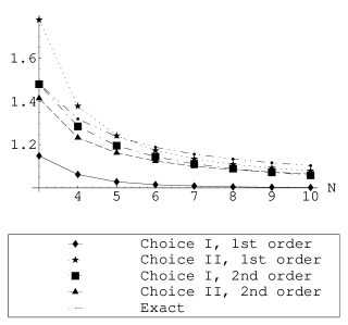
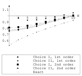
Figure 16: Different results for $m_{eff}$.

Figure 17: Different results for $\sqrt{-E}$.

Yet, there is another way to check reliability. We already said FACC could be used as an alternative to PMS to fix $b_{0}$. More precisely, we could use a FACC on both the energy $E$ as the mass gap equation $\frac{\partial E}{\partial M}=0$. Explicitly, define

$$\delta_{E}=\left|\frac{E_{1}x^{-1}-E_{0}}{E_{0}}\right|$$ (99)

measuring the relative correction of the second order on the first order contribution. The closer $\delta_{E}$ is to 1, the better it is, as an indication that the series expansion is under control. The quantity $\delta_{M}$ is defined in a similar fashion. Unfortunately, no $b_{0}$ exists such that $\left|\frac{\partial\delta_{E}}{\partial b_{0}}\right|$ or $\left|\frac{\partial\delta_{M}}{\partial b_{0}}\right|$ are zero or minimal. However, we can substitute our PMS results in $\delta_{E}$ and $\delta_{M}$ and find out what these give.

Consulting FIG.18 and FIG.19, we are able to understand why we should have ended up with qualitatively good results, since $\delta_{E}$ as well as $\delta_{M}$ are close to 1, even for small $N$. We also see that both choices for $\overline{\mu}$ should give comparable results, since $\delta_{E}$ and $\delta_{M}$ fit with each other.

We also fixed $b_{0}$ by demanding that $\left|\frac{\partial E}{\partial b_{0}}\right|$ was minimal , and we found that results were less good than those obtained by fixing $b_{0}$ by means of $M$, except for small $N$ values . However, the convergence to the exact results for growing $N$ was very slow. For example with Choice I, $Q(5)=19.4\%$, $Q(10)=19.1\%$, $Q(20)=14.1\%$.
An analogous story held true for $m_{eff}$, where $b_{0}$ was determined by demanding that $\left|\frac{\partial m_{eff}}{\partial b_{0}}\right|$ was minimal. There, the deviation from the exact results was always bigger , and the convergence was again rather slow. For example, with Choice I, $P(5)=30.1\%$, $P(10)=25.7\%$, $P(20)=18.5\%$.

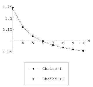
Figure 18: $\delta_{E}$ as a function of $N$.

Figure 19: $\delta_{M}$ as a function of $N$.

All this corroborates our conjecture that $M$ is indeed the best quantity to fix $b_{0}$.

Before we formulate our conclusions, we just like to mention that also in case of $N=2$ there exist a mass gap and a non-perturbative vacuum energy. We already pointed out why we probably didn’t find an optimal $b_{0}$ with our method. The best we can do with this special $N$ value, is just choosing a (physical) renormalization scheme, but we must realize we can easily obtain highly over- or underestimated values in this case and that this is not a self-consistent way to obtain results.

VII Conclusion

This paper, which had the purpose to investigate the dynamical mass generation and non-perturbative vacuum energy of the two-dimensional Gross-Neveu field theory, consisted of two main parts. In the first part, we proved how all bubble Feynman diagrams can be consistently resummed up to all orders in an effective mass $\overline{m}$. We showed that this $\overline{m}$ can be calculated from the gap equation $\frac{\partial E}{\partial\overline{m}}=0$, whereby $E$ is the vacuum energy. $E$ is given by the sum of the $2PPI$ vacuum bubbles, calculated with the $2PPI$ massive propagator (i.e. with mass $\overline{m}$), plus an extra term, accounting for a double counting ambiguity.

We showed that the $2PPI$ expansion can be renormalized with the original counterterms of the model.

A very important fact is that the $2PPI$ expansion for $E$ is only correct if the gap equation $\frac{\partial E}{\partial\overline{m}}=0$ is fulfilled. In this context, we discussed the renormalization group equation for $E$, and showed why $E$ doesn’t obey its RGE order by order, because the requirement of the gap equation turns terms of different orders into the same order. We stress that this does not mean $E$ doesn’t obey its RGE, or ask for the introduction of a ”non-perturbative” $\beta$-function.

To get actual values for $m_{eff}$ and $E$, we employed the $\overline{MS}$ scheme, and after the classical choice $\overline{\mu}=\overline{m}$ to cancel logarithms, we recovered the $N\rightarrow\infty$ results. However, the corresponding coupling constant was infinite, so we couldn’t say anything about validity of the results, without the foreknowledge of exact values. This, combined with the uselessness of the RGE for $E$ to improve calculations, compelled us to search for a more sophisticated way to improve the $2PPI$ technique.

In the second part, we first eliminated the freedom in the renormalization of the $2PPI$ mass parameter, by transforming $\overline{m}$ to a renormalization scheme and scale independent $M$. The consistency relation $\frac{\partial E}{\partial\overline{m}}=0$ was completely equivalent to $\frac{\partial E}{\partial M}=0$. Secondly, we parametrized the coupling constant renormalization. After a reorganization of the series, all scheme dependence was reduced to a single parameter $b_{0}$, equivalent to the choice of a certain scale parameter $\Lambda$.
We fixed this $b_{0}$ by means of the principe of minimal sensitivity (PMS). Originally, PMS was founded on the logical requirement that observable physics cannot depend on how one chooses to renormalize. Translated to our case, $E$ and $m_{eff}$ shouldn’t depend on the arbitrary parameter $b_{0}$. But we showed on theoretical grounds why applying PMS on neither $m_{eff}$ nor $E$ would be valid, because analogously as $E$ ($m_{eff}$) doesn’t lose its scale dependence order by order, it doesn’t lose its scheme dependence order by order.

Nevertheless, we gave an outcome to the problem of PMS. By construction, $M$ is scheme and scale independent, so we can apply PMS on this mass parameter. This provides us with an optimal $b_{0}$ to calculate $M$, and consequently $E$ and $m_{eff}$. For the scale $\overline{\mu}$, we made 2 reasonable choices. These 2 choices gave acceptable results at first order, yet there was quite a big difference between them. The second order results were comparable and qualitatively good, converging to the exact values for growing $N$.

The relevant expansion parameter was relatively small. We gave extra evidence why results were good, by using a fastest apparent convergence argument.

We explicitly checked that using PMS on $E$ and $m_{eff}$ to fix $b_{0}$ gave worse results, and the convergence was very slow.

Summarizing, we have constructed a self consistent method to calculate the mass gap and non-perturbative vacuum energy. The $2PPI$ expansion, as well as the optimization procedure, are immediately generalizable to other field theories.

References

- (1) D.J. Gross, A. Neveu, Phys.Rev. D10 (1974) 3235
- (2) P. Forgács, F. Niedermayer, P. Weisz, Nucl.Phys. B367 (1991) 123
- (3) Al.B. Zamolodchikov, unpublished. See Arvanitis .
- (4) H. Verschelde, K. Knecht, K. Van Acoleyen, M. Vanderkelen, Phys.Lett. B516 (2001) 307
- (5) C. Arvanitis, F. Geniet, M. Iacomi, J.-L. Kneur, A. Neveu, Int.J.Mod.Phys. A12 (1997) 3307
- (6) H. Verschelde, S. Schelstraete, M. Vanderkelen, Z.Phys. C76 (1997) 161
- (7) K. Van Acoleyen, H. Verschelde, Phys.Rev. D65 (2002) 085006
- (8) H. Verschelde, M. Coppens, Phys.Lett. B287 (1992) 133
- (9) H. Verschelde, Phys.Lett. B497 (2001) 165
- (10) H. Verschelde, J. De Pessemier, Eur.Phys.J. C22 (2002) 771
- (11) G. Smet, T. Vanzielighem, K. Van Acoleyen, H. Verschelde, Phys.Rev. D65 (2002) 045015
- (12) J. Baacke, S.Michalski, hep-ph/0210060
- (13) J.A. Gracey, Nucl. Phys. B341 (1990) 403
- (14) J.F. Bennett, J.A. Gracey, Nucl. Phys. B563 (1999) 390
- (15) J.A. Gracey, Nucl. Phys. B367 (1991) 657
- (16) C. Luperini, P. Rossi, Ann. Phys. 212 (1991) 371
- (17) W. Celmaster, R.J. Gonsalves, Phys.Rev. D20 (1979) 1420
- (18) G. Grunberg, Phys.Rev. D29 (1984) 2315
- (19) P.M. Stevenson, Phys.Rev. D23 (1981) 2916