Varying Fundamental Constants from a String-inspired Brane World Model

Abstract

We report results on the construction of cosmological braneworld models in the context of the Einstein-Gauss-Bonnet gravity, which include the leading correction to the Einstein-Hilbert action suggested by superstring theory. We obtain and study the equations governing the dynamics of the standard cosmological models. We find that they can be written in the same form as in the case of the Randall-Sundrum model but with time-varying four-dimensional gravitational and cosmological constants. Finally, we discuss the cosmological evolution predicted by these models and their compatibility with observational data.

guessConjecture

1 Introduction

Many of the cosmological scenarios nowadays under study have been largely originated from theoretical advances in high-energy physics. Of special interest is the study of the new scenarios motivated by developments in string and M theories, where the spacetime has non-compact extra-dimensions. One of the most studied models has been proposed by Randall and Sundrum (RS) [1]. In the RS model all matter and gauge fields, with the exception of gravity, are confined in a 3-brane embedded in a five-dimensional (5D) spacetime, the bulk, with a $\dZ_{2}$ symmetry (with respect to the 3-brane). It has been shown that the zero-mode of the Kaluza-Klein dimensional reduction is localized around the 3-brane, reproducing Newtonian gravity in the weak field approximation. However, the RS model does not include any higher-curvature correction predicted by string theories. Of particular importance is the Gauss-Bonnet term, which is the quadratic correction allowed in order to have a ghost-free action [2, 3]. Moreover, in 5D spacetimes the most general Lagrangian producing second-order field equations is the combination of the Einstein-Hilbert and Gauss-Bonnet terms [4]. Following the motivation provided by these facts we have studied how the dynamics of the standard cosmological models, the Friedmann-Lemaître-Robertson-Walker (FLRW) models, is modified by the introduction of the Gauss-Bonnet term [5].

2 Basic ingredients of the model

The field equations that one obtains from the modification of the RS model by the Gauss-Bonnet term are (see [5] for details):

$$G_{AB}+\Lambda g_{AB}+\alpha H_{AB}=\kappa^{2}\left[-\lambda\tilde{g}_{AB}+T_{AB}\right]\delta(w)~{}~{}~{}(\Lambda<0)\,,$$ (1)

where

$$H_{AB} = RR_{AB}-2R_{A}{}^{C}R_{BC}-2R^{CD}R_{ACBD}+R_{A}{}^{CDE}R_{BCDE}$$

$$-\textstyle{1\over 4}g_{AB}(R^{2}-4R^{CD}R_{CD}+R^{CDEF}R_{CDEF})\,,$$

$\tilde{g}_{AB}$ is the 3-brane metric, $T_{AB}$ is the energy-momentum tensor of the matter confined on the 3-brane ($w=0$) ($T_{AB}n^{B}=0=\tilde{g}_{AB}n^{B}$), and $\lambda$ is a constant that coincides with the brane tension in the limit $T_{AB}=0=\alpha$. According to studies in string theory [3], the fundamental constant $\alpha$ should be positive. To study how the FLRW models behave in our theory we assume: (i) $T_{AB}$ is of the perfect-fluid type

$$T_{AB}=(\rho+p)u_{A}u_{B}+p\tilde{g}_{AB}\,,$$

with $u^{A}$, $\rho$, and $p$, being the fluid velocity ($u^{A}u_{A}=-1$), energy density and pressure respectively. (ii) The 5D line element has the following form (introduced in [6]):

$$ds^{2}=-n^{2}(t,y)dt^{2}+a^{2}(t,y)h_{ij}(k,x^{l})dx^{i}dx^{j}+b^{2}(t,y)dy^{2}\,.$$ (2)

Here $y$ is coordinate in the fifth dimension and $h_{ij}$ is a three-dimensional maximally symmetric metric for the surfaces $\{t={\rm const.},y={\rm const.}\}$, whose spatial curvature is parametrized by $k=-1,0,1\,.$ Then, every spacelike hypersurface $y={\rm const.}$ has a FLRW metric.

The solutions of (1,2) in the bulk for which a limit in Einstein gravity exists are given by (see [5] for details)

$$\textstyle{\dot{a}\over a}\textstyle{n^{\prime}\over n}+\textstyle{a^{\prime}\over a}\textstyle{\dot{b}\over b}-\textstyle{\dot{a}^{\prime}\over a}=0\,,~{}\Phi+\alpha\Phi^{2}=\textstyle{\Lambda\over 6}+C(\textstyle{a_{i}\over a})^{4}\,,~{}\Phi=\frac{\dot{a}^{2}}{a^{2}n^{2}}-\frac{a^{\prime 2}}{a^{2}b^{2}}+\frac{k}{a^{2}}\,.$$

where $C$ is an integration constant and $a_{i}$ is a constant that later we will use as the initial scale factor on the 3-brane, which will represent the freedom in the choice of the initial time.

Given the bulk spacetime, there are two important ingredients in the geometrical construction of a braneworld model: the embedding of the 3-brane and the implementation of the $\dZ_{2}$ symmetry. This can be done by following the same procedure used in the matching of two spacetimes in General Relativity, where two spacetimes with boundary are glued by using a one-to-one identification of the points in the boundaries. Now, the two spacetimes will be described by the metric (2), one with $y\leq 0$, say $V^{-}$, and the other one with $y\geq 0$, say $V^{+}$. For both spacetimes, the boundary considered is the hypersurface $y=0$, where the 3-brane will be located. Now, instead of identifying only the boundaries of $V^{+}$ and $V^{-}$ we can identify all the points of $V^{+}$ with those of $V^{-}$ in the following way: $(x^{\alpha},y)\leftrightarrow(x^{\alpha},-y)$. With this we establish how these spacetimes have to be matched and, at the same time, we implement the $\dZ_{2}$ symmetry.

With regard to the 3-brane, the metric that it inherits from $V^{+}$ and $V^{-}$ is the same, as expected. However, the extrinsic curvatures differ by a sign, due to the $\dZ_{2}$ symmetry, and hence the normal derivative of the braneworld metric has a jump across the 3-brane. This jump can be determined in terms of energy-momentum distribution on the 3-brane [see the right-hand side of Eq. (1)]. To that end, one has to use find the junction conditions corresponding to our theory, which are different from those in General Relativity. This requires to formulate the field equations in the sense of distributions and to take special care of some terms coming from the Gauss-Bonnet term (details will be given in [7]). Following this procedure for the geometries we have considered (2), and considering only the solution with a proper limit $\alpha\rightarrow 0$, we arrive at the following modified Friedmann equation for the Hubble function $H=\dot{a}_{o}/(n_{o}a_{o})$:

$$H^{2}=\frac{1}{3}\tilde{\kappa}^{2}_{\ast}\rho\left(1+\frac{\rho}{2\lambda}\right)-\frac{k}{a^{2}_{o}}+\frac{1}{3}\tilde{\Lambda}_{\ast}\,.$$ (3)

Here, the 4D gravitational coupling and cosmological constants, $\tilde{\kappa}_{\ast}$ and $\tilde{\Lambda}_{\ast}$ respectively, are time dependent. Actually, they change in time as functions only of the scale factor $a_{o}$. Their explicit form is

$$\tilde{\kappa}^{2}_{\ast} = \frac{\tilde{\kappa}^{2}}{1+\varepsilon(\frac{a_{i}}{a_{o}})^{4}}\,,~{}~{}\tilde{\kappa}^{2}\equiv\frac{\lambda\kappa^{4}}{6\chi^{2}}\,,~{}~{}\varepsilon\equiv\frac{4\alpha C}{\chi^{2}}\,,~{}~{}\chi\equiv\sqrt{1+\textstyle{2\over 3}\alpha\Lambda}$$

$$\tilde{\Lambda}_{\ast} = \frac{\lambda}{2}\frac{\tilde{\kappa}^{2}}{1+\varepsilon(\frac{a_{i}}{a_{o}})^{4}}-\frac{3}{2\alpha}\left(1-\chi\sqrt{1+\varepsilon(\frac{a_{i}}{a_{o}})^{4}}\right)$$

The only formal difference between the Friedmann equation (3) and the corresponding RS equation is that the dark radiation term [8] proportional to $a^{-4}_{o}$ does not appear explicitly. It has been included in $\tilde{\Lambda}_{\ast}$. Actually, at zero order in $\alpha$ we have: $\tilde{\Lambda}_{\ast}=\tilde{\Lambda}_{RS}+3Ca^{-4}_{o}+O(\alpha)\,,$ and we recover the Friedmann equation corresponding to RS braneworlds (see, e.g., [9]). Moreover, in analogy to the RS case, $\tilde{\kappa}^{2}$ is the 4D gravitational coupling constant.

As in standard cosmology, the Friedmann equation (3) together with the energy-momentum tensor conservation equations [a consequence of the divergence-free character of the left-hand side of (1)],

$$\dot{\rho}=-3(\rho+p)H\,,$$

and a barotropic equation of state $p=p(\rho)$, describe completely the cosmological dynamics on the brane.

The explicit form of the bulk solution has been presented in [5], for the case in which the fifth dimension is assumed static ($\dot{b}=0$). This solution is a 5D black hole spacetime which in the limit $\alpha\rightarrow 0$ coincides with the 5D Schwarzschild-AdS black hole. We have also found that the integration constant $C$ is proportional to the black hole mass.

3 Cosmological dynamics

Let us now analyze some questions about the behaviour of the FLRW models according to this theory. For a general analysis see [5]. Here, we will be interested in the high-energy regime, where our theory deviates significantly from General Relativity (GR).

That regimes occurs at very early times, where we would expect a large contribution from the bulk curvature, i.e. $\varepsilon(\frac{a_{i}}{a_{o}})^{4}\gg 1$. In this situation the Friedmann equation can be approximated by

$$H^{2}\simeq\frac{\tilde{\kappa}^{2}}{3\varepsilon}\left[\rho(1+\frac{\rho}{2\lambda})+\frac{\lambda}{2}\right](\frac{a_{o}}{a_{i}})^{4}+\frac{\tilde{k}^{2}\lambda}{6}\frac{\chi}{1-\chi}\sqrt{\varepsilon}(\frac{a_{i}}{a_{o}})^{2}\,.$$ (4)

Following the general belief that the expansion of the Universe went through an early stage of positive acceleration, let us assume that that the Hubble function, for small $a_{o}/a_{i}$, behaves as $H^{2}\sim(a_{o}/a_{i})^{-n}$ ($n\leq 2$). If we take $n=2$ we get zero acceleration (which corresponds to the behaviour of the Milne Universe). On the other hand, if we take $n=0$, we get the scale factor of the de Sitter model, which grows exponentially in time. From our approximation (4), we can see that in order to have a positive acceleration, the first term on the right-hand side should dominate at some stage, and should have an expansion index $n<2$. In general, this is not possible at very early times, where the second term with an expansion index $n=2$, would dominate. According to this, we could expect that the Universe had an initial quasi-Milne phase driven by geometry and afterwards a positive acceleration driven by, for instance, a scalar field. Then, in these models, an inflationary stage would be shifted in time. Moreover, they also have the interesting property that the particle horizon will be logarithmic divergent, since the Milne Universe doesn’t have any horizon. This fact could suggest an alternative mechanism to solve the horizon problem, even if we still require an accelerated era.

Let us now look at the Big-Bang Nucleosynthesis (BBN) and supernova constraints for our model. First, it is clear that in the limit $\varepsilon=0$ the cosmology will be the standard one. A surprise arises when one wants to study the BBN constraint in the strong bulk-curvature regime. Indeed, assuming that $1/\lambda$ and $\varepsilon(\frac{a_{i}}{a_{o}})^{4}$ were large enough, the Hubble function would behave as follows

$$H^{2}\simeq\frac{\tilde{k}^{2}a_{o}^{4}}{6\varepsilon\lambda a_{i}^{4}}\rho^{2}\,,$$

then, since during the BBN the dominant energy-density component would be the radiation one, i.e. $\rho\propto a_{o}^{-4}$, this implies that $H^{2}\propto a_{o}^{-4}$, which means that we recover the same dynamical behaviour as in GR. Using the standard BBN calculations [10] it is possible to find a range of parameters compatible with the observations and the requirement that the quadratic part on the energy density be the dominant one.

The second observational constraint we are going to consider is the one imposed by supernovae (SNIa) redshift measurements [11]. If we combine the constraints coming from this data with the previous ones from BBN we get a tiny region where the cosmological constraints are compatible with a strong deviation from the GR behaviour, as it can be seen from Fig.(1). Even if the cosmological constraints are satisfied, the very small magnitude of $\lambda$ is quite suspicious. Indeed in the RS case, from deviation of Newton law in sub-mm experiments, one gets the constraint $\lambda>10^{8}\ GeV^{4}$ [12]. In any case, the implementation of such constraint in this case is still an open question.

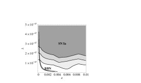
Figure 1: BBN and SNIa constraints to large deviations of our model from the GR one, for $\chi=0.2$ and $a_{i}=1$. The coloured regions from the darker to the white correspond to 1 to 4 $\sigma$ confidence form the SNIa data [11]. BBN and SNIa are in agreement in our model at 2 $\sigma$. $\lambda$ is measured in $GeV^{4}$.

To sum up, we have studied the dynamics of the standard FLRW cosmological models in a theory that generalizes the RS model [1] by taking into account the Gauss-Bonnet higher-order curvature term [3]. We have shown how the equations governing the cosmological dynamics can be written in the same form as those in RS scenarios but with time-dependent 4D gravitational and cosmological constants. Studying the 5D geometry of our model we have found that the time variation of the constants is parametrized only by the mass of a black hole in the bulk. We have also shown that the higher-order curvature terms present in our theory, which are dominant at high energies and change the cosmological dynamics at early times, can provide alternative cosmological scenarios for the study of unsolved cosmological problems. In this sense, we have seen that a strong bulk curvature limit is compatible with BBN [10] and SNIa [11] observational data, and how this could provide alternative solutions to the horizon problem. In this respect, the compatibility of such a model with the constraints imposed by the Newtonian gravity at low energies is still open.

- [1] Randall, L. and Sundrum, R.: 1999, Phys. Rev. Lett. 83, p. 4690
- [2] Zwiebach, B.: 1985, Phys. Lett. B156, p. 315
- [3] Boulware, D. G. and Deser, S.: 1985, Phys. Rev. Lett. 55, p. 2656
- [4] Lovelock, D.: 1971, J. Math. Phys. 12, p. 498
- [5] Germani, C. and Sopuerta, C. F.: 2002, Phys. Rev. Lett. 88, p. 231101-1
- [6] Binétruy, P., Deffayet, C., and Langlois, D.: 2000, Nucl. Phys. B565, p. 269; Binétruy, P., Deffayet, C., Ellwanger, U., and Langlois, D.: 2000, Phys. Lett. B477, p. 285
- [7] Germani, C. and Sopuerta, C. F.: 2002, in preparation
- [8] Maartens R.: 2000, Phys. Rev. D62, p. 084023-1
- [9] Csaki C., Graesser, M., Kolda, C., and Terning, J.: 1999, Phys. Lett. B462, p. 34; Cline, J., Grojean C., and Servant G.: 1999, Phys. Rev. Lett. 83, p. 4245
- [10] Olive, K. A., Steigman, G., and Walker, T. P.: 2000, Phys. Rept. 333, p. 389
- [11] Perlmutter S., et al.: 1999, Astrophys. J. 517, p. 565
- [12] R. Maartens, D. Wands, B. A. Bassett and I. Heard: 2000, Phys. Rev. D 62, p. 04130-1