Fractal Theory Space:
Spacetime of Noninteger Dimensionality

We construct matter field theories in a “theory space” that is fractal, and invariant under geometrical renormalization group (RG) transformations. We treat in detail complex scalars, and discuss issues related to fermions, chirality, and Yang-Mills gauge fields. In the continuum limit these models describe physics in a noninteger spatial dimension which appears above a RG invariant “compactification scale,” $M$. The energy distribution of KK modes above $M$ is controlled by an exponent in a scaling relation of the vacuum energy (Coleman-Weinberg potential), and corresponds to the dimensionality. For truncated-$s$-simplex lattices with coordination number $s$ the spacetime dimensionality is $1+(3+2\ln(s)/\ln(s+2))$. The computations in theory space involve subtleties, owing to the $1+3$ kinetic terms, yet the resulting dimensionalites are equivalent to thermal spin systems. Physical implications are discussed.

1 Introduction

All quests for organizing principles of physics beyond the Standard Model, since the classic era of grand unification in the late 1970’s, have involved extra dimensions. The foremost example is supersymmetry, [1], in which one postulates Grassmanian extra dimensions and graded extensions of the Lorentz group. Supersymmetry and bosonic extra dimensions are essential to the use of string theory with matter fields as a complete description of all forces, including quantum gravity. Motivated by certain viable limits of string theory, [2], the possibility of extra conventional spatial dimensions at the $\sim$ TeV scale, possibly accessible to future colliders, has lately become the focus of a lot of activity. Latticization, [3], or “deconstruction,” [4], of compactified extra dimensional theories provides an effective gauge invariant Lagrangian in $1+3$ dimensions truncated on $N$ KK modes of scalars, fermions and gauge fields in $D$ dimensions. This has provided a point of departure for abstracting a new class of models based upon the notion of “theory space” as emphasized by Arkani-Hamed, Cohen and Georgi [4].

Theory space, without some defining principles, is an empty concept. A key idea we emphasize presently is that theory space can be endowed with certain abstract geometrical symmetries that are essentially renormalization group (RG) transformations. These transformations are distinct from scale transformations and truly reflect a geometric structure of the theory. Geometrical symmetries in continuum extra dimensions therefore become replaced by the renormalization group in theory space. We can thus turn it around and use the RG to generate new kinds of geometries. In the present paper we study a nontrivial example of the latter possibility.

In particular, we will borrow from condensed matter physics certain recursively defined, or fractal, lattices to construct classes of new theory spaces. These lattices are defined by recursively “decorating” a lattice of coordination number, $s$, by replacing each site with a simplex of $s$ sites, preserving the coordination number $s$. This process is iterated an arbitrary number, $k$, times. It results in a lattice, which for us describes a fractal theory space matter field theory. In the $k\rightarrow\infty$ limit it describes a continuum theory whose properties are determined by certain scaling laws of the (zero temperature) quantum theory, analogous to the scaling laws of critical systems at finite critical temperature.

The key observation is that the Feynman path integral for these systems is invariant under a sequence of renormalization group (RG) transformations that map the $k$th lattice into the $k-1$ lattice. In the $k\rightarrow\infty$ limit, this RG invariance imples a certain scaling law for the vacuum action functional, e.g., the Coleman-Weinberg potential. This scaling law, and consistency with the RG transformations imposed as a symmetry, leads to the determination of a “critical exponent,” $\epsilon$. This exponent is associated with the number distribution of KK modes with energy:

$$N(E)\propto\left(\frac{E}{M}\right)^{\epsilon}$$ (1.1)

Here $\epsilon$ is the dimensionality of the extra dimensions; $M$ is a RG invariant mass scale, which is interpreted as the effective “compactification scale.” The effects of the extra dimension show up only for energy scales $E\geq M$ as KK-modes appear. We will obtain irrational (indeed, transcendental) values for $\epsilon$ for the lattices considered presently. Since theory space, endowed with such a geometrical symmetry, is effectively a theory of compact extra dimensions in the continuum limit, we have thus arrived at a prescription for constructing a spacetime field theory in a flat spacetime of noninteger dimensionality. Our construction is essentially a regularization procedure for the theory, which is ultimately defined as a continuum limit. Certain delicacies associated with that limit are discussed, including, e.g., the “Casimir” effects associated with compactification.

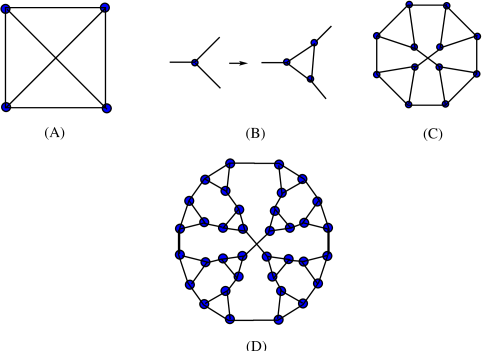
Figure 1: The truncated $3$-simplex lattice. (A) Kernel (complete) lattice with coordination number $3$; (B) the decoration which replaces each site under recursion; (C) the first order decorated lattice; (D) the second order decorated lattice. A theory space can be constructed by defining each site to correspond to a complex scalar $Z|\partial\phi_{a}|^{2}-\mu^{2}|\phi_{a}|^{2}$, and each link to $-\Lambda^{2}|\phi_{a}-\phi_{b}|^{2}$. On the $k$th order truncated $s$-simplex we have the number of sites $N_{k}=(s+1)s^{k}$, and number of links, $L_{k}=(s+1)s^{k+1}/2$.

The kernel lattices we consider are “complete” lattices in which every site corresponds to a complex scalar field theory of mass $\mu$ in $1+3$ dimensions, and every link is a hopping term, $\Lambda^{2}|\phi_{a}-\phi_{b}|^{2}$, coupling every scalar field at every site to every other site. For example, in Fig.(1) we show a complete square kernel, equivalent to a tetrahedron, as a zeroth order kernel lattice with coordination number $s=3$ (this is called the “truncated $3$-simplex”). We then construct the next order lattice by replacing each vertex with a simplex. This integrates in $s-1$ new fields and $s$ new links per original site. In Fig.(1C) we have replaced each site of the kernel with $3$-simplices to produce the first order lattice. We then iterate the replacement to produce the second order lattice of Fig.(1D). The procedure can be iterated $k$ times, and we ultimately imagine $k\rightarrow\infty$ to define a continuum limit. It yields a system of $N_{k}=(s+1)s^{k}$ complex scalar fields coupled through $L_{k}=(s+1)s^{k+1}/2$ links.

The renormalization group transformations that define a symmetry of this system reduce the $k$th order lattice Lagrangian back to the $(k-1)$th order lattice, preserving the Feynman path integral. These are composed of a sequence of “polygon-$\star$” tranformations, analogous to those first discussed by Onsager for the Ising model [8], followed by “$4$-chain $\rightarrow$ $2$-chain dedecorations.” These transformations will be adapted to the $1+3$ field theories that live on sites of the theory space lattice. Such RG manipulations are familiar from the condensed matter literature, but are tricky in theory space in a fundamental way: the deconstructed theory possesses continuum kinetic terms for the field theory in the $1+3$ Lagrangian. We must include renormalization effects on these kinetic terms, up to irrelevant operators that are quartic derivatives, e.g. $(\partial^{2}\phi)^{2}/\Lambda^{2}$. In particular, $|\partial(\phi_{a}-\phi_{b})|^{2}$ must be interpreted as a quartic derivative (we’ll see that discarding this term only affects the high mode number part of the spectrum). These irrelevant operators of the derivative expansion are dropped, and the renormalization of the relevant $|\partial\phi|^{2}$ terms is determined. This renormalization plays a crucial role in the scaling law for the Coleman-Weinberg potential. One obtains the effective Lagrangian in the $(k-1)$th lattice, with parameters that are renormalized under the transformations. The consistency of the RG symmetry, i.e., of the invariance of the Feynman path integral, is realized only for a particular value of the dimensionality, $\epsilon$.

The solution to the problem of extracting $\epsilon$ essentially adapts the scaling theory of critical exponents [5]. We follow closely the beautiful approach of Dhar [6], who also discussed many other lattices, and determined the dimensionality for finite temperature spin systems. The scaling property of the Coleman-Weinberg potential, and the obtained values of $\epsilon$, depend crucially upon the recursive construction of the lattices. Though the physical systems we consider are different than the static spin systems considered by Dhar, and we are working in the zero-temperature quantum theory, we nonetheless recover Dhar’s result for the noninteger dimensionality of the truncated-$s$-simplex lattices of coordination number $s$:

$$\epsilon=\frac{2\ln(s)}{\ln(2+s)}.$$ (1.2)

Moreover, we find that there are additional RG invariants. One of these is a mass scale $M$ which plays the role of the compactification scale of the theory, and arises somewhat mysteriously, much like $\Lambda_{QCD}$ by dimensional transmutation. Below the scale $M$ the theory is governed only by its zero-modes, and lives in the $1+3$ dimensions of the original field theories attached to each site of the lattice. Above $M$ the “KK-modes” begin to appear in the RG invariant distribution of eq.(1.1), which is the main observable of the theory. Another RG invariant leads to the classical “running coupling constant” relationship in $\epsilon$ dimensions, $g^{2}\propto(E/M)^{\epsilon}$.

When we go over to theories involving fermions and Yang-Mills fields there are various subtleties. We describe these mostly qualitatively in Section 4. Despite these subtleties, it appears that a Standard Model generalization can be constructed in $1+(3+\epsilon)$ dimensions. In the Conclusions we will address some options to the question of physical interpretation.

2 Transformations for Deconstructed Lattice Fields

We begin by considering transformations which augment or thin the degrees of freedom of $1+3$ theories of many complex scalar fields. These transformations stem from symmetries noticed long ago in the Ising model, [7, 8, 9]. In the language of Ising models a single spin₁-link-spin₂ combination in the Hamiltonian can always be “decorated,” i.e., written as a spin₁-link-spin^′-link-spin₂ interaction. That is, we can “integrate in” the new spin^′, or “decorate” the original single link. Thus, an $N$-spin system can be viewed as a $2N$ spin system upon decorating. The decorations can be arbitrarily complicated, involving many new spins. Conversely, we can “integrate out” or “dedecorate” the spins internal to a chain whose endpoint spins are then renormalized (Fig.(2)).

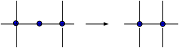
Figure 2: The $3$-chain $\rightarrow$ $2$-chain dedecoration transformation integrates out the internal field and renormalizes the endpoint fields’ kinetic terms and mass terms.

Decoration is an exact scale transformation for Ising spins, and continuous spins (e.g., “spherical models” are spin systems which correspond to our models in the absence of kinetic terms). Presently we are dealing with a transverse lattice [10] in which our “spins” are fields that have $1+3$ kinetic terms. For us decoration and dedecoration transformations are exact scale transformations only in the limit of very large cut-off $\Lambda$. This occurs because we perform decoration transformations truncating on quartic derivatives, such as $|\partial^{2}\phi_{a}|^{2}/\Lambda^{2}$. This is, nonetheless, a good approximate transformation in the $\Lambda\rightarrow\infty$ limit, or for the low lying states in the spectrum. These transformations become symmetries when the theory is classically scale invariant, i.e., $\mu^{2}=0$ and $\Lambda\rightarrow\infty$, and when combined with polygon-$\star$ transformations (below) on the recursively defined fractal lattices, they become geometric symmetries for arbitrary $\mu^{2}\neq 0$, i.e., a fixed renormalized $\mu^{2}$ can be defined. The $1+3$ kinetic terms undergo renormalizations under these transformations, and thus distinguish the present construction from that of a spin model (e.g., the continuous complex spherical model).

We will also require a generalization of Onsager’s “star-triangle” or more generally, “polygon-$\star$” transformations that replace a complete polygon of spins, Fig.(3), with a radiating star configuration, integrating in a new centroid spin. This transformation can again be done in field theory to leading order in the derivative expansion, provided the plaquette is not oriented (which creates a complication when we attempt to include fermions and gauge fields). The polygon-$\star$ transformations are, thus, only exact for us in the $\Lambda\rightarrow\infty$ limit. There will generally be hidden symmetries associated with the new centroid field which may play a role in application to gauge or chiral–fermion theories.

The key result is that combining sequences of polygon-$\star$ and dedecoration transformations allows us to map a recursively defined truncated $s$-simplex lattice at $k$-th order into the same lattice at $k-1$ order with different physical parameters. This leads to the renormalization group as a geometric symmetry in the large $k$ limit. The invariance of the Coleman-Weinberg potential in the large $k$ limit allows us to determine the dimensionality of the theory. This limit corresponds to $\Lambda\rightarrow\infty$, and corrections to the result after truncating the derivative expansion are vanishing. The surviving RG invariant parameters allow us to interpret this as a geometric, as opposed to a scale, transformation.

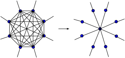
Figure 3: The polygon-$\star$ transformation for a complete hexagon deletes the intrahexagonal links, and integrates in a new central field with radial links out the endpoint fields.

2.1 Dedecoration Transformations

2.1.1 Example: 3-chains $\rightarrow$ $2$-chains

We warm up with the simplest example of a “dedecoration transformation” applied to chains of complex scalar fields. This corresponds to a scale transformation on the theory; it is a symmetry of the theory only if $\mu\rightarrow 0$. When $\mu\rightarrow 0$ we will see that the spectra before and after the dedecoration transformation coincide in the low energy (low mode number) limit.

Consider an $N$ complex scalar field Lagrangian in $1+3$, which can be viewed as a deconstructed $S_{1}$ compactified extra dimension with periodic boundary conditions:

$${\cal{L}}=Z_{0}\sum^{N}_{a=1}|\partial\phi_{a}|^{2}-\Lambda_{0}^{2}\sum^{N}_{a=1}|\phi_{a}-\phi_{a+1}|^{2}-\mu_{0}^{2}\sum^{N}_{a=1}|\phi_{a}|^{2}$$ (2.3)

where we take $N$ to be even and assume periodicity, hence $\phi_{N+a}=\phi_{a}$. It is convenient to allow for noncanonical normalization of the kinetic terms, and we thus display the arbitrary wave-function renormalization constant $Z_{0}$.

It is useful to consider ${\cal{L}}$ as a sum over 3-chains:

$${\cal{L}}=\sum^{N-1}_{n\;odd}{\cal{L}}_{n,n+2}$$ (2.4)

Each 3-chain involves three fields. The first 3-chain is:

$${\cal{L}}_{1,3}=\frac{1}{2}Z_{0}(|\partial\phi_{1}|^{2}+2|\partial\phi_{2}|^{2}+|\partial\phi_{3}|^{2})-\Lambda_{0}^{2}|\phi_{1}-\phi_{2}|^{2}-\Lambda_{0}^{2}|\phi_{2}-\phi_{3}|^{2}-\frac{1}{2}\mu_{0}^{2}(|\phi_{1}|^{2}+2|\phi_{2}|^{2}+|\phi_{3}|^{2})$$ (2.5)

The fields $\phi_{1}$ and $\phi_{3}$ share half their kinetic terms and $\mu^{2}$ terms with the adjacent chains, thus carry the normalization factors of $1/2$ within the chain (more generally, the endpoint fields may have $s-1$ links with other fields and thus carry $1/s$ factors in the kinetic and mass terms of each chain). $\phi_{2}$ can be viewed as a “decoration” of the chain. We can integrate out the internal field $\phi_{2}$ and obtain an equivalent renormalized chain. Integrating out $\phi_{2}$:

$${\cal{L}}_{1,3}=\frac{1}{2}Z_{0}(|\partial\phi_{1}|^{2}+|\partial\phi_{1}|^{2})-(\Lambda_{0}^{2}+\frac{1}{2}\mu_{0}^{2})(|\phi_{1}|^{2}+|\phi_{3}|^{2})+\Lambda_{0}^{4}(\phi_{1}+\phi_{3})^{\dagger}\frac{1}{Z_{0}\partial^{2}+2\Lambda_{0}^{2}+\mu_{0}^{2}}(\phi_{1}+\phi_{3})$$ (2.6)

Expanding in the derivatives and regrouping terms gives:

$${\cal{L}}_{1,3}=\frac{1}{2}Z_{1}(|\partial\phi_{1}|^{2}+|\partial\phi_{3}|^{2})-\Lambda_{1}^{2}|\phi_{1}-\phi_{3}|^{2}-\frac{1}{2}\mu_{1}^{2}(|\phi_{1}|^{2}+|\phi_{3}|^{2})-\delta_{1}|\partial(\phi_{1}-\phi_{3})|^{2}+{\cal{O}}(\partial^{4}/\Lambda^{2})$$ (2.7)

where we obtain:

$$Z_{1} = Z_{0}\frac{8\Lambda_{0}^{4}+4\Lambda_{0}^{2}\mu_{0}^{2}+\mu_{0}^{4}}{4\Lambda_{0}^{4}+4\Lambda_{0}^{2}\mu^{2}+\mu_{0}^{4}}\approx 2Z_{0}$$

$$\Lambda_{1}^{2} = \frac{\Lambda_{0}^{4}}{2\Lambda_{0}^{2}+\mu_{0}^{2}}\approx\frac{1}{2}\Lambda_{0}^{2}$$

$$\mu_{1}^{2} = \frac{2\mu_{0}^{2}\Lambda_{0}^{2}+\mu_{0}^{4}}{2\Lambda_{0}^{2}+\mu_{0}^{2}}\approx\mu_{0}^{2}$$

$$\delta_{1} = \frac{Z_{0}\Lambda_{0}^{4}}{(2\Lambda_{0}^{2}+\mu_{0}^{2})^{2}}\approx\frac{1}{4}Z_{0}$$ (2.8)

We have written the approximate forms of the renormalizations of the parameters in the large $\Lambda$ limit. Note that the $\mu^{2}$ term is multiplicatively renormalized. This owes to the fact that it is the true scale-breaking term in the theory when the lattice is taken very fine, and $\Lambda$ terms become derivatives, i.e., as $\mu\rightarrow 0$ the theory has a zero-mode. Since it alone breaks the symmetry of scale-invariance, elevating the zero-mode, it is therefore multiplicatively renormalized in free field theory.

The $\delta$ term has been written in the indicated form because, though it superficially appears to be a relevant $d=4$ operator, it too is a quartic derivative on the lattice, i.e., ($\partial^{2}$ in $1+3$) $\times$(a nearest neighbor hopping term on the lattice). It effects only the high mass limit of the KK mode spectrum. It is therefore dropped for consistency with the expansion to order $\partial^{4}/\Lambda^{2}$.

The fields develop a new wave-function renormalization constant $Z_{1}$. Note that in the $\Lambda>>\mu$ limit, $Z_{1}\rightarrow 2Z_{0}$, twice the original normalization. This renormalization is common to all the $\phi_{a}$ fields in the other chains. Thus, we can write the original theory with $N$ fields as a sum over the renormalized 2-chains, containing a total of $N/2$ fields:

$${\cal{L}}^{\prime}=Z_{1}\sum^{N/2}_{a=1}|\partial\phi_{a}|^{2}-\Lambda_{1}^{2}\sum^{N/2}_{a=1}|\phi_{a}-\phi_{a+1}|^{2}-\mu_{1}^{2}\sum^{N/2}_{a=1}|\phi_{a}|^{2}$$ (2.9)

The dropping of the $|\partial(\phi_{a}-\phi_{b})|^{2}$ terms, which appear to be superficially relevant, affects only the high energy spectrum of eq.(2.9) when $\mu=0$ in the limit $\Lambda\rightarrow\infty$ and $N\rightarrow\infty$, holding $M=\Lambda/N$ fixed. To see this, we diagonalize eq.(2.3) to obtain the mass spectrum:

$$m^{2}_{0}(n)=Z_{0}^{-1}\Lambda_{0}^{2}\sin^{2}(\pi n/N)+Z_{0}^{-1}\mu_{0}^{2}\qquad n=(0,1,..,N-1)$$ (2.10)

Diagonalizing eq.(2.9) yields the mass spectrum:

$$m^{2}_{1}(n)=Z_{1}\Lambda_{1}^{2}\sin^{2}(2\pi n/N)+Z_{1}^{-1}\mu_{1}^{2}\qquad n=(0,1,..,N-1)$$ (2.11)

and comparing with eqs.(2.8) we see that $m^{2}_{1}(n)\approx m^{2}_{0}(n)$ for $n<<N$, if we neglect the $\mu^{2}$ terms. The renormalized mass term $Z_{1}^{-1}\mu_{1}^{2}=(1/2)Z_{0}^{-1}\mu_{0}^{2}$, is halved by the dedecoration transformation, and thus we have performed a scale transformation on the original theory. The two spectra coincide in the small $n$ limit of the scale-invariant theory with $\mu^{2}=0$.

Viewed as a renormalization group, we see that the large $N$ system flows under repeated application of dedecoration transformations to a block-spin thinned theory $N^{\prime}<<N$ with $\mu\rightarrow 0$, which is the scale invariant fixed point.

2.1.2 Renormalized $4$-chains $\rightarrow$ $2$-chains

We will require in our applications presently the reduction of slightly more general 4-chains, which are two endpoint fields and 2 internal decorating fields. We must allow for a more general parameterization of the chain fields, since this structure will arise on the lattices of interest after a polygon-$\star$ transformation (below). Generally, after performing polygon-$\star$ transformations on our lattice, the full Lagrangian will be a sum over $4$-chains of the form:

$${\cal{L}}^{full} = \sum_{n}{\cal{L}}_{n}^{4-chain}$$ (2.12)

These $4$-chains will live on lattices with a coordination number $s$ and generally have different normalizations for the two endpoint fields than the two internal fields:

$${\cal{L}}^{4-chain} = \frac{1}{s}Z_{\Phi}|\partial\Phi_{1}|^{2}+Z_{\phi}|\partial\phi_{1}|^{2}+Z_{\phi}|\partial\phi_{2}|^{2}+\frac{1}{s}Z_{\Phi}|\partial\Phi_{2}|^{2}$$ (2.13)

$$-\frac{1}{s}\mu_{0}{}^{2}(|\Phi_{1}|^{2}+s|\phi_{1}|^{2}+s|\phi_{2}|^{2}+|\Phi_{4}|^{2})$$

$$-\Lambda^{\prime}_{0}{}^{2}|\Phi_{1}-\phi_{1}|^{2}-{\Lambda}_{0}^{2}|\phi_{1}-\phi_{2}|^{2}-\Lambda^{\prime}_{0}{}^{2}|\Phi_{2}-\phi_{2}|^{2}$$

The endpoint $\Phi_{i}$ fields are shared with $s-1$ other neighboring chains, hence the $Z_{\Phi}/s$ kinetic term normalization, and the $\mu_{0}^{2}/s$ factors. Furthermore, note the central link for the internal fields, $|\phi_{1}-\phi_{2}|^{2}$, has a different strength ${\Lambda_{0}}^{2}\neq\Lambda^{\prime}_{0}{}^{2}$ than the extremity links.

We integrate out the internal scalars $\phi_{1}$ and $\phi_{2}$. This requires diagonalizing the $\phi_{1}$-$\phi_{2}$ internal (mass)² matrix, which has eigenvalues $\Lambda^{\prime}_{0}{}^{2}$ and $\Lambda^{\prime}_{0}{}^{2}+2\Lambda_{0}{}^{2}$. We then regroup the derivative terms as before, discarding quartic and higher derivatives. We thus obtain a renormalized $2$-chain:

$${\cal{L}}^{2-chain}=\frac{\tilde{Z}}{s}(|\partial\Phi_{1}|^{2}+|\partial\Phi_{2}|^{2})-\tilde{\Lambda}^{2}|\Phi_{1}-\Phi_{2}|^{2}-\frac{\tilde{\mu}^{2}}{s}(|\Phi_{1}|^{2}+|\Phi_{2}|^{2})+{\cal{O}}(\partial^{4}/M^{2})$$ (2.14)

where:

$$\tilde{Z} = Z_{\Phi}+{sZ\Lambda^{\prime}_{0}{}^{4}}\left[\frac{1}{(\Lambda^{\prime}_{0}{}^{2}+\mu_{0}{}^{2})^{2}}\right]$$

$$\tilde{\Lambda}^{2} = {\frac{1}{2}\Lambda^{\prime}_{0}{}^{4}}\left[\frac{1}{(\Lambda^{\prime}_{0}{}^{2}+\mu_{0}{}^{2})}-\frac{1}{(\Lambda^{\prime}_{0}{}^{2}+2\Lambda_{0}^{2}+\mu_{0}{}^{2})}\right]$$

$$\tilde{\mu}^{2} = \mu_{0}{}^{2}\frac{(1+s)\Lambda^{\prime}_{0}{}^{2}+\mu_{0}{}^{2}}{\Lambda^{\prime}_{0}{}^{2}+\mu_{0}{}^{2}}$$ (2.15)

It is useful to define the ratio $\kappa=\Lambda^{\prime}_{0}{}^{2}/\Lambda_{0}^{2}$ and consider the large $\Lambda$ limit of these expressions:

$$\tilde{Z} \rightarrow {Z_{\Phi}}+Zs$$

$$\tilde{\Lambda}^{2} = {\Lambda^{\prime}_{0}{}^{2}}\frac{\kappa}{(\kappa+2)}$$

$$\tilde{\mu}^{2} = \mu_{0}{}^{2}(1+s)$$ (2.16)

We will find that $4$-chains arising after polygon-$\star$ transformations on the truncated $s$-simplex lattices will have $\kappa=s$.

The full Lagrangian after replacing the $4$-chains by the $2$-chains and summing over all $2$-chains, will take the form:

$${\cal{L}}^{full} = \tilde{Z}\sum_{a}|\partial\Phi_{a}|^{2}-\tilde{\mu}{}^{2}\sum_{a}|\Phi_{a}|^{2}-\tilde{\Lambda}{}^{2}\sum_{a,b}|\Phi_{a}-\Phi_{b}|^{2}$$ (2.17)

Note that when the $2$-chains are summed, the $1/s$ factors disappear in overall kinetic and mass term normalizations.

2.2 Polygon-$\star$ Transformations

Let us consider a “complete” deconstructed Lagrangian for a polygon of $s$ sites. This is a highly nonlocal structure of Fig.(3) in which all sites are linked to all other sites with a common bond strength:

$${\cal{L}}^{polygon}=Z_{0}\sum^{s}_{a=1}|\partial\phi_{a}|^{2}-\frac{1}{2}{\Lambda_{0}^{2}}\sum^{s}_{a=1}\sum^{s}_{b=1}|\phi_{a}-\phi_{b}|^{2}-\mu_{0}^{2}\sum^{s}_{a=1}|\phi_{a}|^{2}$$ (2.18)

Note that we must be careful not to double count, the link $|\phi_{a}-\phi_{b}|^{2}$ in double sums, hence the factors of $1/2$. It is interesting to compute the mass spectrum of the perfect polygon by itself, going into the Fourier basis:

$$\phi_{a}=\frac{1}{\sqrt{s}}\sum^{s-1}_{k=0}e^{\pi ika/s}\chi_{n};\qquad\phi_{a+s}=\phi_{a}$$ (2.19)

whence:

$${\cal{L}}=Z_{0}\sum^{s-1}_{k=0}|\partial\chi_{k}|^{2}-s\Lambda_{0}^{2}\sum^{s-1}_{k=1}|\chi_{k}|^{2}-\mu_{0}^{2}\sum^{s-1}_{k=0}|\chi_{k}|^{2}$$ (2.20)

Note the sum in the second term begins at $k=1$, so the mode $k=0$ is a zero mode when $\mu=0$. Hence, renormalizing $\Lambda^{2}=\Lambda_{0}^{2}/Z_{0}$ and $\mu^{2}=\mu_{0}^{2}/Z_{0}$, the spectrum, consists of $s-1$ degenerate modes of mass $\sqrt{s\Lambda^{2}+\mu^{2}}$, and the single mode of mass $\mu$ with $k=0$.

The polygon of $s$ complex scalar fields admits a transformation which introduces a central complex scalar field $\Phi$ and becomes the $s$-star with $(s+1)$ complex scalar fields. Let us consider the $\star$ action in the form:

$${\cal{L}}^{\star}=Z_{\Phi}|\partial\Phi|^{2}+Z\sum^{s}_{a=1}|\partial\phi_{a}|^{2}-\Lambda^{\prime}{}^{2}\sum^{s}_{a=1}|\Phi-\phi_{a}|^{2}-\mu^{2}_{\Phi}|\Phi|^{2}-\mu^{\prime}{}^{2}\sum^{s}_{a=1}|\phi_{a}|^{2}$$ (2.21)

Note that all $|\phi_{a}-\phi_{b}|^{2}$ bonds have been deleted and we introduce new $|\Phi-\phi_{a}|^{2}$ bonds radiating from the central scalar $\Phi$.

Starting with ${\cal{L}}^{\star}$, we integrate out $\Phi$:

$${\cal{L}}^{\star} = Z\sum^{s}_{a}|\partial\phi_{a}|^{2}-(\Lambda^{\prime}{}^{2}+\mu^{\prime}{}^{2})\sum^{s}_{a}|\phi_{a}|^{2}$$ (2.22)

$$\qquad+\left[\Lambda^{\prime}{}^{4}\sum^{s}_{a,b}\phi_{a}^{\dagger}\frac{1}{Z_{\Phi}\partial^{2}+s\Lambda^{\prime}{}^{2}+\mu_{\Phi}^{2}}\phi_{b}+h.c.\right]$$

Performing the derivative expansion and reorganizing terms, we thus recover the polygon form of the Lagrangian:

$${\cal{L}}^{\star}\rightarrow{\cal{L}}^{polygon} = Z_{0}\sum^{s}_{a}|\partial\phi_{a}|^{2}-\frac{1}{2}{\Lambda_{0}^{2}}\sum^{s}_{a,b}|\phi_{a}-\phi_{b}|^{2}-\mu_{0}^{2}\sum^{s}_{a}|\phi_{a}|^{2}+{\cal{O}}(\frac{\partial^{2}}{\Lambda^{2}})$$

and we have the relations:

$$Z_{0} = Z+Z_{\Phi}\frac{s\Lambda^{\prime}{}^{4}}{(s\Lambda^{\prime}{}^{2}+\mu_{\Phi}^{2})^{2}}\approx Z+\frac{Z_{\Phi}}{s}$$

$$\Lambda_{0}^{2} = \frac{\Lambda^{\prime}{}^{4}}{(s\Lambda^{\prime}{}^{2}+\mu_{\Phi}^{2})}\approx\frac{\Lambda^{\prime}{}^{2}}{s}$$

$$\mu_{0}^{2} = \frac{(\mu_{\Phi}^{2}+s\mu^{\prime}{}^{2})\Lambda^{\prime}{}^{2}+\mu_{\Phi}^{2}\mu^{\prime}{}^{2}}{(s\Lambda^{\prime}{}^{2}+\mu_{\Phi}^{2})}\approx\mu^{\prime}{}^{2}\frac{(s+1)}{s}$$ (2.24)

where the approximate expressions hold in the large $\Lambda$ limit, and are all that we ultimately require to implement the renormalization group.

Note that we have freedom within the ${\cal{L}}^{\star}$ Lagrangian to vary the ratios $Z_{\Phi}/Z$ and $\mu_{\Phi}/\mu^{\prime}$. We can for example, choose $Z_{\Phi}=0$, in which case $\Phi$ is a nonpropagating auxiliary field. The $\Phi$ field will recover a kinetic term when subsequent chain transformations are performed. The $Z_{\Phi}=0$ case is interesting for Yang-Mills, and corresponds to “integrating in” an infinite coupling constant gauge field, and the infinite coupling will run to a finite value after subsequent chain transformations. Presently we will make the convenient choice $\mu^{\prime}{}^{2}=\mu_{\Phi}^{2}$, but we do not specify explicitly $Z_{\Phi}/Z$. This will act as a check on our result.

We can readily invert the transformation in the large $\Lambda$ limit. In summary, the polygon Lagrangian:

$${\cal{L}}^{polygon}=Z_{0}\sum^{s}_{a=1}|\partial\phi_{a}|^{2}-\frac{1}{2}{\Lambda_{0}^{2}}\sum^{s}_{a=1}\sum^{s}_{b=1}|\phi_{a}-\phi_{b}|^{2}-\mu_{0}^{2}\sum^{s}_{a=1}|\phi_{a}|^{2}$$ (2.25)

can be replaced by the $\star$ Lagrangian:

$${\cal{L}}^{\star}=Z_{\Phi}|\partial\Phi|^{2}+Z\sum^{s}_{a=1}|\partial\phi_{a}|^{2}-\Lambda^{\prime}{}^{2}\sum^{s}_{a=1}|\Phi-\phi_{a}|^{2}-\mu^{\prime}{}^{2}|\Phi|^{2}-\mu^{\prime}{}^{2}\sum^{s}_{a=1}|\phi_{a}|^{2}$$ (2.26)

with the choice of parameters $(\Lambda\rightarrow\infty)$:

$$\frac{Z_{\Phi}}{s}+Z = Z_{0}$$

$$\Lambda^{\prime}{}^{2} = s\Lambda_{0}^{2}$$

$$\mu^{\prime}{}^{2} = \mu_{0}^{2}\frac{s}{s+1}$$ (2.27)

2.3 Combining Polygon-$\star$ and $4$-chain Transformations to Reduce the Truncated $s$-simplex Lattice

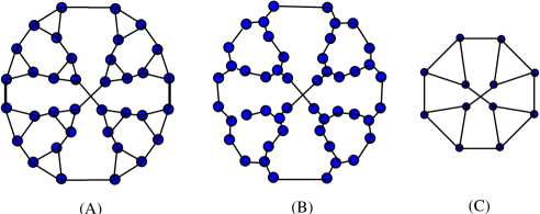
Figure 4: Illustration of $k$$\rightarrow$$k-1$ RG transformation. (A) Second ($k$th) order truncated $3$-simplex; (B) reduced after polygon(triangle)-$\star$ transformations; (C) reduced to first ($k-1$) order after $4$-chain $\rightarrow$ $2$-chain transformations.

We are now ready to construct the RG transformation for the truncated-$s$-simplex lattice by combining the above transformations. Consider any $k$th order $s$-simplex lattice built up recursively as described in Section I. For concreteness consider Fig.(4A), the second order $3$-simplex.

The Lagrangian of the $k$th order lattice takes the form:

$${\cal{L}}_{k}=Z_{0}\sum^{N_{k}}_{a=1}|\partial\phi_{a}|^{2}-\Lambda_{0}^{2}\sum^{L_{k}}_{links}|\phi_{a}-\phi_{b}|^{2}-\mu_{0}^{2}\sum^{N_{k}}_{a=1}|\phi_{a}|^{2}$$ (2.28)

We begin by performing the polygon-$\star$ transformations on each of the elementary polygons. All of the elementary polygons are annihilated by this procedure, replaced by stars, and the lattice of Fig.(4A) is carried into that of Fig.(4B). The centers of the stars are connected to neighbors through 4-chains, and the full Lagrangian is now a sum over $4$-chains. We have the $4$-chain parameters determined by eq.(2.27):

$$\frac{Z_{\Phi}}{s}+Z = Z_{0}$$

$$\Lambda^{\prime}{}^{2} = s\Lambda_{0}^{2}$$

$$\mu^{\prime}{}^{2} = \mu_{0}^{2}\frac{s}{s+1}$$ (2.29)

Now we reduce the $4$-chains to $2$-chains. The lattice is mapped from Fig(4B) into Fig.(4C). We see that we have now reduced the original $k$th order lattice to the $k-1$ order with the new Lagrangian:

$${\cal{L}}_{k-1}=\tilde{Z}\sum^{N_{k-1}}_{a=1}|\partial\phi_{a}|^{2}-\tilde{\Lambda}^{2}\sum^{L_{k-1}}_{links}|\phi_{a}-\phi_{b}|^{2}-\tilde{\mu}^{2}\sum^{N_{k-1}}_{a=1}|\phi_{a}|^{2}$$ (2.30)

The parameters renormalize as in eq.(2.16) where $\kappa=\Lambda^{\prime}{}^{2}/\Lambda{}^{2}=s$. The resulting overall renormalization is:

$$\tilde{Z} = sZ_{0}$$

$$\tilde{\Lambda}^{2} = {\Lambda_{0}^{2}}\frac{s}{(s+2)}$$

$$\tilde{\mu}^{2} = \mu_{0}^{2}s$$

$$\tilde{N}\equiv N_{k-1} = \frac{N_{k}}{s}$$ (2.31)

We have also noted the change in the number of fields, $N_{k}$. We see that the arbitrariness of choosing ${Z_{\Phi}}/Z$ (also, $\mu_{\Phi}/\mu^{\prime}$, which we fixed to unity) in the intermediate step is a hidden symmetry in the result.

3 Computation of the Dimensionality

3.1 Vacuum Energy Scaling Law

We have described a theory of free complex scalars defined on the $k$th iteration of the kernel lattice. For the truncated-$s$-simplex lattices the coordination number is $s$, the number of fields in the $k$th iteration is $N_{k}=(s+1)(s)^{k}$ and the number of links is $L_{k}=(s+1)s^{k+1}/2$. The Lagrangian is:

$${\cal{L}}=Z\sum^{N_{k}}_{a=1}|\partial\phi_{a}|^{2}-\Lambda^{2}\sum^{L_{k}}_{a,b}|\phi_{a}-\phi_{b}|^{2}-\mu^{2}\sum^{N_{k}}_{a=1}|\phi_{a}|^{2}$$ (3.32)

where the linking mass term sums over the links.

If we could Fourier transform eq.(3.32) we would obtain a mass spectrum of the form $M_{n}^{2}=\omega^{2}_{n}+\mu^{2}$. The path integral for our theory then takes the form in a Euclidean momentum space, up to an overall multiplicative normalization factor:

$$e^{-\Gamma}=\int D\phi\;e^{-\int d^{4}x{\cal{L}}}=\prod_{p_{\mu}}\prod_{n=1}^{N_{k}}(Zp^{2}+\omega_{n}^{2}+\mu^{2})^{-1}$$ (3.33)

The vacuum energy, or Coleman-Weinberg potential, is up to an overall additive constant:

$$\Gamma=Z^{-2}\int\frac{d^{4}p}{(2\pi)^{4}}\sum_{n}\ln(p^{2}+\omega_{n}^{2}+\mu^{2})$$ (3.34)

where we have rescaled the $4$ momentum integral by $Z$.

We want to replace the sum on $n$ by a continuous momentum integral. In any integer dimensionality, $n$ is a vector, $\vec{n}=(n_{x},n_{y},...)$. We want to perform the angular integral in the sum over discrete $\vec{n}$. This leaves a sum over the radial magnitude of $n=\sqrt{\vec{n}\cdot\vec{n}}$ with a dimension-dependent measure. In $\epsilon$ dimensions if we interpret $n$ as the radial magnitude, then in the continuous approximation to the sum we can replace:

$$\sum_{n=0}^{N_{k}}\rightarrow\frac{1}{\epsilon}\int_{0}^{N_{k}}dn(n/N_{k})^{\epsilon-1}$$ (3.35)

In replacing the discrete sum by a continuous integral we will induce “Casimir effect” corrections to the vacuum energy. These are discussed in the Appendix.

With $n$ a radial coordinate, the leading behavior at low $n$ of $\omega^{2}_{n}$ is $\omega^{2}_{n}\sim c(n/N_{k})^{2}\Lambda^{2}$, where $c$ is a constant (e.g., $c=\pi^{2}$ in a one dimensional periodically compactified situation). Let us rescale $n$ to write the integral over an $4+\epsilon$ dimensional momentum vector,

$$p^{2}=p_{\mu}p^{\mu}+c(n/N_{k})^{2}\Lambda^{2}$$ (3.36)

The Coleman-Weinberg potential becomes:

$$\Gamma=c(\epsilon)\frac{Z^{-2}N_{k}}{\Lambda^{\epsilon}}\int\frac{d^{4+\epsilon}p}{(2\pi)^{4+\epsilon}}\ln(p^{2}+\mu^{2})$$ (3.37)

Here $c(\epsilon)$ is an overall normalizing factor coming from the $c$ dependence, the ratio of the $d=4$ to $d=4+\epsilon$ solid angles and $(2\pi)^{d}$ normalizing factors. This factor is irrelevant for the scaling argument, but given by:

$$c(\epsilon)=\frac{1}{\epsilon}\left(\frac{4\pi}{c}\right)^{\epsilon/2}\Gamma(2+\epsilon/2)$$ (3.38)

The integral, apart from the explicit scaling prefactor, is finite for nonzero $\epsilon$. It is thus insensitive to $k$ as $k\rightarrow\infty$ to its UV cut-off limit and to $\Lambda\rightarrow\infty$. We discuss this integral and the limiting procedure in greater detail in the Appendix. Performing the integral:

$$\Gamma=\frac{Z^{-2}N_{k}}{\Lambda^{\epsilon}}(\mu)^{4+\epsilon}V(\epsilon)$$ (3.39)

where $V(\epsilon)$ is insensitive to $k$ as $k\rightarrow\infty$.

Thus, suppose we know the value of the parameters $Z$, $\mu$, $\Lambda$ and $N_{k}$ for some large value of $k$. Then, we obtain the Coleman-Weinberg potential for $k-1$ by the sequence of RG transformations and we find new parameters:

$$\tilde{Z}=h(s)Z,\qquad\tilde{\mu}=f(s)\mu,\qquad\tilde{\Lambda}=g(s)\Lambda\qquad N_{k-1}=N_{k}/s.$$ (3.40)

Since $V$ is insensitive to $k$ for $k\rightarrow\infty$ (and large $\Lambda$) we have:

$$Z^{-2}\frac{N_{k}}{\Lambda^{\epsilon}}(\mu)^{4+\epsilon}=\frac{(\tilde{Z})^{-2}N_{k-1}}{(\tilde{\Lambda})^{\epsilon}}(\tilde{\mu})^{4+\epsilon}$$ (3.41)

or:

$$1=\frac{(f(s))^{4+\epsilon}}{s(h(s))^{2}(g(s))^{\epsilon}}$$ (3.42)

and thus the dimensionality is determined as:

$$\epsilon=\frac{(-4\ln(f(s))+\ln(s)+2\ln(h(s)))}{\ln(f(s)/g(s))}$$ (3.43)

3.2 Dimensionality and RG Invariants of the Trucated-$s$-simplex Lattices

Let us compute the dimensionality of the truncated $s$-simplex lattices. From eqs.(2.31) we have:

$$h(s)=s,\qquad f(s)=\sqrt{s},\qquad g(s)=\sqrt{\frac{s}{s+2}}.$$ (3.44)

The dimensionality is thus:

$$\epsilon=\frac{2\ln(s)}{\ln(s+2)}$$ (3.45)

We have recovered the result of Dhar for the dimensionality of spin-systems on the truncated $s$-simplex lattices. In Dhar’s analysis of spins systems, the spins are static, i.e., have no kinetic terms in an auxiliary $1+3$ dimensions. The wave-function renormalizations are essential in our present renormalization group and to the scaling law for the Coleman-Weinberg potential. Nonetheless, the lattice dimensionality is the same as in the static spin system.

Note that the coordination number must satisfy $s>2$ for a nontrivial noninteger dimensionality. For $s=2$ the dimension is always $1$. For the truncated $s$-simplex lattices we have $1\leq\epsilon\leq 2$.

The scaling laws amongst the four quantities of eqs.(2.31) imply that there are $3$ invariants. We have just encountered one invariant from the vacuum energy scaling law, and there are thus two others. We list them as follows:

$${V}_{r} = \frac{(\tilde{Z})^{-2}N_{k-1}}{(\tilde{\Lambda})^{\epsilon}}(\tilde{\mu})^{4+\epsilon}$$

$$\mu_{r}^{2} = \frac{\tilde{\mu^{2}}}{\tilde{Z}}$$

$$N_{r} = \tilde{Z}\tilde{N}$$ (3.46)

It is useful to define a noninvariant renormalized cut-off:

$$\Lambda_{r}^{2}=\frac{\tilde{\Lambda}^{2}}{\tilde{Z}}$$ (3.47)

$\Lambda_{r}$ can be used as the “running” mass scale, or identified with the energy scale of interest, $E\sim\Lambda_{r}$.

In contrast to the case of the $3$-chain$\rightarrow$$2$-chain dedecoration acting on a chain of $N$ scalars, the present RG transformation is not a scale transformation. We see that the renormalized mass $\mu_{r}$ is invariant under the RG transformation. The present RG transformation is a statement about the geometric recursive structure of the theory. This RG invariance of $\mu_{r}$ emboldens us to consider this as a symmetry of a novel continuum theory.

Combining $\mu_{r}$ with the RG invariant vacuum energy scaling factor $V_{r}$ allows us to define yet another RG invariant mass scale:

$$M=\frac{\tilde{\Lambda}_{r}}{(\tilde{N})^{1/\epsilon}}$$ (3.48)

The scale $M$ is fixed in the large $\Lambda_{r}$ and $\tilde{N}$ limit, and has nothing to do with the physical mass ${\mu}_{r}$. It defines the threshold scale of the KK-modes, i.e., the effective compactification scale of the theory. Comparing with the spherically symmetric measure in the integral of eq.(3.35) we see that the number of KK modes with energy $E$ is given by

$$n(E)=\left(\frac{E}{M}\right)^{\epsilon}$$ (3.49)

$M$ is therefore the “compactification” scale of the noninteger extra dimension. The scale $M$ persists in the $\mu\rightarrow 0$ limit. It is somewhat mysterious, in that we are taking a classical theory to a continuum limit, yet a nontrivial RG invariant mass scale survives. It is a consequence of the fact that the dimensionality is not trivial, i.e., $\epsilon\neq 0$ and a fundamental scale must survive since the trace of the stress tensor is presumably nonzero in this classical theory. In this sense, $M$ is analogous to $\Lambda_{QCD}.$ For us $\epsilon$ is classical, while in QCD $\epsilon\sim\beta/g$ is an anomalous dimension.

The physical significance of the invariance of $\tilde{Z}\tilde{N}$ pertains to interacting theories, such as Yang-Mills gauge theories. We can identify:

$$\tilde{Z}\propto\frac{1}{g^{2}}$$ (3.50)

a common dimensionless coupling constant of the deconstructed theory defined at the scale of the cut-off. Then the invariant $M$ tells us how the coupling constant scales with choice of cut-off. To see the running coupling constant scaling law combine eq.(3.48) and eq.(3.50) to obtain:

$${g^{2}(E)}\propto\left(\frac{E}{M}\right)^{\epsilon}$$ (3.51)

Thus, we recover normal power-law running of $g^{2}(\Lambda_{r})$ when $\epsilon$ takes on integer values. The formula exhibits the generalization for noninteger dimension.

We have made a continuous approximation to the integrals, but we can always “rediscretize” the sum in an RG invariant way. The original choice of the definition of the energy, $\omega_{n}=\sqrt{c}n\Lambda/N_{k}$ is not RG invariant. We see that the overall coefficient of the Coleman-Weinberg potential in eq.(3.36) can be written as:

$$\frac{Z^{-2}N_{k}}{\Lambda^{\epsilon}}(\mu)^{4+\epsilon}=(\mu_{r})^{4+\epsilon}M^{-\epsilon}$$ (3.52)

Hence, rediscretizing, we replace

$$M^{-\epsilon}\int d^{4+\epsilon}p\;I(p)\sim\int d^{4}p\sum_{n}(n)^{\epsilon-1}I(p_{\mu},\omega_{n})$$ (3.53)

and the energy of the $n$th mode is $\omega_{n}=\sqrt{c}nM$.

The difference between the rediscretized sum, taken to infinity, and the continuous integral, is a Casimir effect. In the Appendix we show that the Casimir effect can be expressed as a finite integral. The finite integral is vanishing when we assume that the theory can be expressed in a $4+\epsilon$ dimensional Lorentz invariant way. It is not necessary to make this strong assumption; the effects of the noninteger extra dimension may show up in an RG invariant way only at the threshold scale $M$, but have bad non-RG invariance at higher energies. This depends upon the physical interpretation of the theory. The finiteness of the Casimir integrals suggest to us that a true RG invariant theory exists, and our construction for any finite order of $k$ is just a regulator with RG-symmetry breaking terms.

4 Considerations of Gauge Fields and Fermions

Naturally, we are interested in realistic models built along the lines suggested here. Thus we will require Yang-Mills, and fermions, including chirality. The present discussion will be qualitative, as we note some new issues that arise in attempting this extension.

When we go over to theories involving fermions and Yang-Mills fields there are additional subtleties. These subtleties revolve around the polygon-$\star$ transformation. For example, Wilson fermions in a polygon cannot be mapped to the $\star$ configuration. Similarly, the PNGB’s of Yang-Mills theories that are periodically compactified must be lifted by plaquettes in order to perform the polygon-$\star$ transformation. The point is that the polygon is orientable, while the $\star$ is not, so orientational elements of the action will not be carried through by the transformation. In the Yang-Mills case, an arbitrary magnetic flux threading a plaquette, $\int B\cdot dA\sim\oint A\cdot dx$ cannot be represented by the $\star$ form of the action, and this requires that a certain PNGB be infinitely heavy. The $\star$ configuration, however, will be seen to be the key to creating chiral fermions. Chiral fermions in deconstruction are lattice defects. In the present case they must be incorporated as the centers of $\star$ configurations that are invariant under the RG transformations used to reduce the lattice. In a sense then, chiral fermions are rarified defects, or invariant centers in the fractal lattice, similar to doping atoms in a material, or to the centers of snowflakes.

Yang-Mills gauge fields are introduced in a deconstructed theory by having gauge groups, $G_{a}$, living on sites and linking-Higgs-fields defined on links. We also include plaquette terms which show up as mass terms of PNGB’s in the $1+3$ dimensions. Hence, let us choose $G_{a}=SU(N)$ with a common coupling constant $g$, and the link field $\Phi_{ab}$ is then an $(\overline{N},N)$ chiral field with a VEV, $\left\langle\Phi\right\rangle=vI_{N}$. The Lagrangian is then:

$${\cal{L}}_{YM}=-\sum_{n=1}^{N_{k}}\frac{1}{4g^{2}}G^{a}_{\mu\nu}G^{a}{}^{\mu\nu}+\sum_{(ab)}^{L_{k}}\mathop{\rm Tr}[D_{\mu},\Phi_{ab}]^{\dagger}[D^{\mu},\Phi_{ab}]+\sum_{plaq\;n}^{P_{k}}\lambda_{n}\mathop{\rm Tr}[\prod_{plaq\;n}\Phi_{ab}]$$ (4.54)

The irreducible plaquettes are those which do not encircle a subplaquette (i.e., can be contracted). The irreducible plaquettes are $P_{k}=(s+1)^{k+1}$.

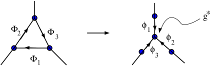
Figure 5: The triangle-$\star$ transformation for an irreducible plaquette maps $\Phi_{i}\rightarrow\phi_{j}$, but imposes a constraint, $\Phi_{3}\Phi_{2}\Phi_{1}=1$.

${\cal{L}}_{YM}$ has been supplemented with a plaquette action, where each plaquette has a coupling constant $\lambda_{k}$. Let us first consider $\lambda_{k}=0$. Then the theory will contain a spectrum of $1$ vector zero mode, $N_{k}-1$ massive gauge fields (KK-modes), and in tree approximation $L_{k}-N_{k}+1$ massless PNGB’s. The PNGB’s will generally be lifted in perturbation theory to masses of order $\alpha M^{2}$, but they can also be elevated by turning on the $\lambda_{k}$. Indeed, we see that $P_{k}>>L_{k}$, so including all irreducible plaquettes with large $\lambda_{n}$ we can lift all PNGB’s, except for a single zero-mode.

Lifting the PNGB’s is necessary for the implementation of the $\star$-chain RG. In Fig.(5) we see a mapping of the irreducible triangle with link fields $\Phi_{i}$ into a star configuration with new link fields $\phi_{j}$. The net gauge phase rotations in going from one site to another must be faithfully represented under this redefinition, thus:

$$\Phi_{1}=\phi_{3}^{\dagger}\phi_{2}\qquad\Phi_{2}=\phi_{1}^{\dagger}\phi_{3}\qquad\Phi_{3}=\phi_{2}^{\dagger}\phi_{1}$$ (4.55)

and we thus see that the $\Phi_{i}$ are constrained:

$$1=\Phi_{3}\Phi_{2}\Phi_{1}$$ (4.56)

This is the orientability problem mentioned above. It requires the quantization of the Wilson loop around the triangle plaquette $g\oint A_{A}dx^{A}=2\pi n$ (more properly, $\Phi_{3}\Phi_{2}\Phi_{1}$ must lie in the center of the group). In the deconstruction language, it imposes a constraint on the PNGB’s. We can treat this constaint by introducing terms $\sim\lambda_{123}\mathop{\rm Tr}(\Phi_{3}\Phi_{2}\Phi_{1})$ for all elementary plaquettes, and we treat $\lambda_{n}$ as a Lagrange multiplier, then perform the polygon-$\star$ transformation. This will lift the PNGB’s from the spectrum. This is the expected decoupling that of high mass PNGB’s must occur when the short-distance degrees of freedom are thinned. Thus, we expect that polygon-$\star$ transformations should make sense in the theory with plaquettes.

An intriguing point is that the $\star$ Lagrangian involves “integrating in” additional Yang-Mills gauge groups at the centers of stars with coupling constants $g^{\star}$. As we saw in the star transformation, there is a freedom to choose the wave-function renormalization constant, $Z_{\Phi}$, arbitarily relative to its neighbors. This translates into the freedom of choosing the coupling constant $g^{*}$ for the new central gauge group arbitrarily. In particular, we can choose $g^{*}=\infty$, which completely suppresses the continuum kinetic term of the new gauge field at this scale. The subsequent chain transformations will induce a finite coupling and gauge invariant kinetic term for this gauge field as we perform the $4$-chain$\rightarrow$$2$-chain transformations. The renormalized couplings after the combined transformations for all gauge fields will have a common value and will run according to the scaling laws described in the previous section.

Barring topological obstructions, we thus expect that the reduction for Yang-Mills gauge fields goes through in the Gaussian approximation. We obtain the same dimensionality as for complex scalars. Obviously the question of the effects of interactions is of great importance. We expect that there are $1+3$ continuum renormalization group effects that accompany the lattice reduction, which corresponds to a change of scale (e.g., of $\Lambda_{r}$). The main issue, however, comes from the power-law running in eq.(3.51). The Yang-Mills coupling constant as described classically, will reach evolving upward with scale, a unitarity bound, $g^{2}\sim(4\pi)^{2}$ at an effective scale $\Lambda_{r}^{\star}$ fairly quickly (it would be interesting to construct models in which $\epsilon<<1$ where the power law running is suppressed, and appears approximately logarithmic). This is the scale of unitarity breakdown for longitudinal KK-mode scattering [3]. This would imply a phase transition in the theory, possibly the string transition. Another logical possibility is that $g^{2}$ runs large, but then is “reset” to a small value by a dynamical transition in the theory, then runs large again, etc., leading to a limit cycle. With a limit cycle it may be possible to take $\Lambda_{r}\rightarrow\infty$ in the interacting theory as well, without a transition to the string phase. Perhaps the most interesting possibility is that the theory has a UV fixed point [12], which may arise between a competition of the classical running and the one-loop correction.

Fermions pose additional challenges. Fermions live on sites and will have kinetic “hopping terms” on the links. We can always view the lattice as a fermion mass matrix, take all fermions to be vectorlike, and choose the hopping terms to be mass terms. This would readily admit polygon-$\star$ transformations and RG reduction of the lattice as we have derived. This would seem to us to be a relatively uninteresting case.

The hopping terms should be built out of $\gamma$ matrices. We expect that we require the use of all $\gamma$ matrices through $\gamma_{4+[s/2])}$ in construction of the action. Hence, for $s=2$, $\gamma_{5}$ suffices, such as in $S_{1}$, while $s=3$ requires $\gamma_{6}$, etc. Consider the polygon of Fig.(5) for $s=3$ the fermionic hopping terms around the perimeter of the polygon. Using $\gamma_{5}$, the hopping terms are of the form $\sum_{n}v\overline{\psi}_{n}\gamma_{5}\Phi_{n}\psi_{n+1}$. Generally this form leads to the fermion doubling problem [11], but admits polygon-$\star$ transformations. It is most sensible to consider Wilson fermions [11] (the Wilson fermion structure will always occur with SUSY). With Wilson fermions the hopping terms are written as $\sum_{n}(v\overline{\psi}_{nL}\Phi_{n}\psi_{(n+1)R}-v\overline{\psi}_{nR}\psi_{nR})$. The Wilson fermion hopping terms have a definite orientational sense, $L(n)\rightarrow R(n+1)$, around the polygon. These cannot be reduced by polygon-$\star$ transformations, and it is not clear to us that sensible reducible fermionic actions exist which are compatible with the polygon-$\star$ transformation. It should be borne in mind, however, that the polygon-$\star$ transformation is ultimately a convenience in computing the dimensionality of the lattice. More exotic fermionic reductions that do not require the polygon-$\star$ transformation may exist.

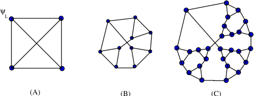
Figure 6: The truncated $3$-simplex lattice constructed with an invariant star dislocation for chirality. (A) Kernel (complete) lattice with coordination number $3$ and a single chiral fermion attached to the upper lh site; (B) the first order decoration replaces each site under recursion except the invariant star; (C) the second order decorated lattice. A theory space can be constructed by defining each site to correspond to a vectorlike Standard Model, except the invariant star which is the usual chiral Standard Model. Hopping terms involve gauge links and Dirac fermion mass terms, $\overline{\psi}_{a}\psi_{b}+h.c.$. The chiral fermions in the invariant star have chiral hops $\overline{\psi}_{L}\psi_{bR}+h.c.$ to the vectorlike neighbors. The zero-mode structure of the theory is the chiral Standard Model.

If we use an action with vectorlike fermions and fermionic Dirac mass matrix hopping terms, $\overline{\Psi}_{a}\Psi_{b}+h.c.$, we can still introduce chirality. We must construct “invariant stars,” i.e., dislocations in the lattice that are not reduced by the RG transformations as in Fig.(6). At the center of the invariant star configuration we introduce a single chiral fermion, $\Psi_{L}$. The fermion has radial hopping terms to the perimeter fermions of the form $\sum_{n}v\overline{\Psi}_{L}\phi_{n}\psi_{nR}$. By “doping” a mass-matrix lattice with the appropriate number of chiral dislocations one can construct a fractal imbedding of the Standard Model.

5 Physical Interpretations and Conclusions

How do we interpret these new theories physically? Fractional extra dimensions are not obviously compactified extra dimensions, since no global boundary condition is introduced which corresponds to a global compactification. Rather, we introduced initially a regulator, $\Lambda$, which is our (inverse) lattice scale. We ultimately imagine the limit $\Lambda\rightarrow\infty$, but how this limit is taken is dependent upon the physical interpretation of the theory. The analogue of a compactified theory emerges with the determination of a compactification scale, the RG invariant $M$, and is a physical scale held fixed in the $\Lambda\rightarrow\infty$ limit. $M$ would still be present, however, with a different definition of the theory in which we maintain a finite $\Lambda$, and we may have a hierarchy $M<<\Lambda$, in analogy to the usual compactified extra dimensional theories.

There are thus two physical interpretations for these constructions. The first is an “outer” modification of spacetime. Here we have in mind finite $\Lambda$ but a dimensional transition at the scale $M<<\Lambda$ in which we view the continuous $1+3$ dimensions as a brane in a higher dimension with a surface structure with characteristic scale length $1/M$. This brane surface is viewed as dynamical, analogous to surfaces in condensed matter physics, and may arise from an interface with an exterior region involving new physics. The fractal theory space is an effective description of such a system on scales not far above $M$. The fractality, in analogy with surface layers on material media, may arise because the interface with the extra outside dimensions involves a region of rapid change in physical parameters. In this picture Lorentz invariance at short distances strictly only applies to the $1+3$ dimensions, but with $\Lambda$ large the relevant low energy physics of the dimensional transition scale $M$ is approximately Lorentz invariant in $1+(3+\epsilon)$ dimensions. In this case, the scale $\Lambda$ may represent a further higher energy transition to string theory. Terms of order $\Lambda^{4}$ and $\Lambda^{2}\mu^{2}$ reflecting the finite cut-off will be present in the vacuum energy, and are non-RG invariant. The low energy physics, however, is a fixed point under these renormalizations that drastically change the UV part of the theory.

The alternative, and perhaps more intriguing view, is an “inner” modification of physics, in that the scale $M$ represents a true dimensional transition to $1+(3+\epsilon)$ dimensions, with enhanced Lorentz invariance on scales above $M$. In this case we take $\Lambda\rightarrow\infty$. Then at all shorter distances the noninteger dimensionality is preserved. This is a remarkable possibility in that a quantum field theory defined in $1+(3+\epsilon)$ dimensions with irrational $\epsilon$ is finite to all orders in perturbation theory. The cut-off scale $\Lambda$ can be taken to infinity with impunity, holding $M$ fixed as the defining dimensional transition scale.

If we were naive, we would speculate that we have given a prescription for the construction of finite quantum field theories of matter. Thus, all infinites in $1+3$ dimensions of the Standard Model would be associated with the cut-off scale $M$, which is the threshold for new physics associated with the noninteger correction to the dimension of space-time. Above the scale $M$ we would begin to include KK-modes in accord with the energy distribution $(E/M)^{\epsilon}$, and we would treat the field theory with ‘t Hooft–Veltman dimensional regularization as the exact calculational tool for $4+\epsilon$ dimensions. Thus, one way to treat the Standard Model as a quasi-noninteger dimensional theory would be to replace all loop integrals in $4$-dimensions by $4+\epsilon$ dimensions above a fixed matching scale $M$:

$$\makebox{Loops}\rightarrow\int_{0}^{M}\frac{d^{4}k}{(2\pi)^{4}}+M^{-\epsilon}\int_{M}^{\infty}\frac{d^{4+\epsilon}k}{(2\pi)^{4}}$$ (5.57)

Modulo ambiguities in treating $\gamma^{5}$, This theory is apparently finite above $M$ to all orders in perturbation theory. We would infer some immediate physical consequences, e.g., that the Higgs boson will receive radiative corrections to its mass from top quark loops:

$$m_{H}^{2}\sim-\frac{3g_{t}^{2}}{8\pi^{2}}M^{2}$$ (5.58)

(or heavier fermions in an extension of the model). Hence, we infer that $M^{2}$ is of order $\sim$ TeV (a “Little Higgs” model can raise the scale to $\sim$ 10 TeV through custodial chiral symmetries).

However, the power-law running of the coupling constant, $g^{2}\sim(E/M)^{\epsilon}$ with $\epsilon>0$, implies that either (1) the theory has a UV fixed point or (2) has a limit cycle or (3) undergoes a phase transition at a strong coupling scale $g^{2}\sim(4\pi)^{2}$. In any case we must account for gravity, and imbedding into string theory would seem to be the most sensible option. This prescription is nonetheless worthy of study, and is a “continuous KK-mode distribution approximation” to any theory that envelops the Standard Model into a noninteger extra dimension $\epsilon$.

We have in mind other applications of these ideas. If the theories at lattice sites live in $1+d$ continuous dimensions, then the full theory has $1+d+\epsilon$ dimensionality. For example, with continuum $1+1$ fields and very large $s$ we can construct a flat $4-\epsilon^{\prime}$ dimensional effective theory. Such theories are classically asymptotically free, but the log dependence on $s$ implies that it would be difficult to construct a natural lattice of the kind we have considered, since $s$ must be taken unnaturally large. It is therefore of interest to enlarge the space of recursively defined lattices to see if natural $4-\epsilon$ dimensions make sense with very small $\epsilon$.

Yet another interesting possibility is to deconstruct the string world-sheet. Weyl invariance may be realized as a discrete RG invariance on a latticized world-sheet with a continuum limit. Then we may be able to find unusual generalizations of the string theory to fractal worldsheets. The consequences for the Weyl constraints on the target space may be interesting.

The key result of this paper is that the renormalization group is dual to geometry. The latter acts in space, and the former acts in theory space. The RG can then be used to reverse engineer unusual new geometries. These fractal geometries exploit quantum mechanics in their construction in a fundamental way. In fact, these realize some of the recent speculations about deconstruction as a means of reconstructing spacetime [4]. Though we are far from a complete theory, e.g., one including gravity, we believe this is fertile territory with potentially nontrivial implications beyond those considered presently.

6 Appendix: Properties of the Vacuum Energy

The vacuum energy integral is most readily computed by differentiating wrt $\mu^{2}$. Define $\Gamma=c(\epsilon)(Z^{-2}N/\Lambda^{\epsilon})V(\mu^{2})$ where $V(\mu^{2})$ is the Euclidean integral:

$$V(\mu^{2})=\int\frac{d^{4+\epsilon}p}{(2\pi)^{4+\epsilon}}\ln(p^{2}+\mu^{2})$$ (6.59)

Then:

$$\frac{\partial}{\partial\mu^{2}}V(\mu^{2})=\int\frac{d^{4+\epsilon}p}{(2\pi)^{4+\epsilon}}\frac{1}{p^{2}+\mu^{2}}=\frac{1}{(4\pi)^{2+\epsilon/2}}(\mu)^{2+\epsilon}{\Gamma(-1-\epsilon/2)}$$ (6.60)

Therefore, integrating wrt $\mu^{2}$, noting the integral vanishes for $\mu=0$ for the $4+\epsilon$ range of interest:

$$V(\mu^{2})=\frac{1}{(4\pi)^{2+\epsilon/2}}(\mu)^{4+\epsilon}\frac{\Gamma(2-\epsilon/2)}{(2+\epsilon/2)(1+\epsilon/2)(\epsilon/2)(1-\epsilon/2)}$$ (6.61)

The integral can be performed directly, without differentiating, but is more tedious. In performing the integral this way we have made two assumptions (1) The RG invariance holds for the system under the integral sign; (2) the integral is Lorentz invariant in $4+\epsilon$ dimensions. When these symmetries are imposed “under the integral” we have the RG invariant theory. Such strong assumptions, while the preferred interpretation of the theory, are not necessary, however.

It is useful to consider the integral before we take the continuum limit. Suppose we do not take the $k\rightarrow\infty$ limit first and perform the integral with a cut-off. Consider, from eq.(3.33) and eq.(3.34) the integral with cutoff $K=\sqrt{c}\Lambda$:

$$V_{K}^{\prime}(\mu^{2})=\int_{0}^{K}\frac{d^{4+\epsilon}p}{(2\pi)^{4+\epsilon}}\frac{1}{(p^{2}+\mu^{2})}$$ (6.62)

Here we have assumed that the finite cut-off is Lorentz invariant in $4+\epsilon$ dimensions. We exponentiate the denominator:

$$V_{K}^{\prime}(\mu^{2})=\int_{0}^{\infty}d\alpha\int_{0}^{K}\frac{d^{4+\epsilon}p}{(2\pi)^{4+\epsilon}}e^{-\alpha(p^{2}+\mu^{2})}$$ (6.63)

The $p^{2}$ integral is then carried out, using the solid angle in $d$ dimensions:

$$\Omega_{d}=\frac{2\pi^{d/2}}{\Gamma(d/2)}$$ (6.64)

we have:

$$V_{K}^{\prime}(\mu^{2})=\frac{1}{(2\pi)^{2+\epsilon/2}}\int_{0}^{\infty}d\alpha\left(\int_{0}^{\infty}-\int_{K^{2}}^{\infty}\right)dp^{2}(p^{2})^{1+\epsilon/2}e^{-\alpha(p^{2}+\mu^{2})}$$ (6.65)

The second term can be approximated:

$$V_{K}^{\prime}(\mu^{2}) = V^{\prime}(\mu^{2})-\frac{1}{(2\pi)^{2+\epsilon/2}}\int_{0}^{\infty}d\alpha(K^{2})^{2+\epsilon/2}e^{-\alpha(K^{2}+\mu^{2})}$$ (6.66)

$$\approx V^{\prime}(\mu^{2})-\frac{1}{(2\pi)^{2+\epsilon/2}}\frac{(K^{2})^{2+\epsilon/2}}{K^{2}+\mu^{2}}$$

hence,

$$V_{K}(\mu^{2}) \approx V(\mu^{2})-\frac{1}{(2\pi)^{2+\epsilon/2}}\mu^{2}{(K^{2})^{1+\epsilon/2}}+{\cal{O}}(K^{2})^{2+\epsilon/2}$$ (6.67)

The procedure of considering $V_{K}^{\prime}(\mu^{2})$ omitted the last quartically divergent piece (when $\epsilon=0$), but keeps the quadratically divergent piece.

These additional terms are associated with the UV cut-off on the theory, $\Lambda=K/\sqrt{c}$. Hence they are not RG invariant. These terms do not obstruct our measurement of the dimensionality of the system. If the system has finite $k$, then the dimensionality we compute from the finite terms is “effective,” applying only near the threshold of KK modes, $\sim M$. The far UV spectrum can thus be considerably modified by the finite $\Lambda$ effects which do not respect the RG invariance.

Clearly we would like to argue that the $4+\epsilon$ dimensional theory exists, and the $k\rightarrow\infty$ limit can be taken. In this case, such terms can be viewed as the finite–$k$ regulator effect spoiling the symmetry of RG invariance in the true theory, much the way a momentum-space cut-off spoils gauge invariance. These terms vary under the RG transformation, so they would be subtracted to define the symmetric theory, much as gauge invariance forces the subtraction of the momentum-space cut-off mass term in the vacuum polarization loop. It is simpler to take the limit under the integral sign, since the resulting integral is finite!

Casimir effects arise in principle in the difference between the continuous approximation to the theory and the discretized sum. The form of these effects depends upon how we define the theory, as described above, and will generally have divergences associated with finite UV cut-off’s that are not RG invariant. However, when we define the theory to be $4+\epsilon$ Lorentz invariant and take the UV cut-off to infinity then the Casimir effects are vanishing.

Consider the original discrete vacuum energy expression:

$$\Gamma=Z^{-2}\int\frac{d^{4}p}{(2\pi)^{4}}\sum_{n}\ln(p^{2}+\omega_{n}^{2}+\mu^{2})$$ (6.68)

The Casimir effect is the difference between the continuum integral approximation and the “staircase” in the discrete sum. This difference is minimized by the best fit continuous approximation to the staircase, but a leading residual contribution remains involving the second derivative of the summand. In our case the leading Casimir correction to the continuous approximation is:

$$\delta\Gamma=\frac{1}{4}\frac{Z^{-2}c\Lambda^{2}}{N^{2}_{k}}\int\frac{d^{4}p}{(2\pi)^{4}}\sum_{n}\left[\frac{2}{(p^{2}+\omega_{n}^{2}+\mu^{2})}-\frac{4\omega^{2}_{n}}{(p^{2}+\omega_{n}^{2}+\mu^{2})^{2}}\right]$$ (6.69)

Note the factor of ${c}\Lambda^{2}/N^{2}_{k}$ arising from $(\partial\omega_{n}/\partial n)^{2}$.

We rescale, and take the continuum Lorentz invariant limit the integral-sum goes over to a $4+\epsilon$ dimesnional integral. We have, by the Euclidean invariance, $\omega^{2}_{n}=[\epsilon/(4+\epsilon)]p^{2}$. Hence:

$$\delta\Gamma=\frac{1}{2}c(\epsilon)\frac{Z^{-2}N_{k}}{\Lambda^{\epsilon}}\left(\frac{c\Lambda^{2}}{N^{2}_{k}}\right)\int\frac{d^{4+\epsilon}p}{(2\pi)^{4+\epsilon}}\left[\left(\frac{4-\epsilon}{4+\epsilon}\right)\frac{p^{2}}{(p^{2}+\mu^{2})^{2}}+\frac{2\mu^{2}}{(p^{2}+\mu^{2})^{2}}\right]$$ (6.70)

The integral is readily performed:

$$\delta\Gamma=\frac{1}{2}(\epsilon)\left(\frac{Z^{-2}N_{k}(\mu)^{4+\epsilon}}{(4\pi)^{2+\epsilon/2}\Lambda^{\epsilon}}\right)\left(\frac{c\Lambda^{2}}{N^{2}_{k}\mu^{2}}\right){\Gamma(-1-\epsilon/2)}\left[\left(\frac{4-\epsilon}{4+\epsilon}\right)+(1+\epsilon/2)\left(\frac{4+3\epsilon}{4+\epsilon}\right)\right]$$ (6.71)

In this result we have the usual RG invariant prefactor ${Z^{-2}N_{k}(\mu)^{4+\epsilon}}/{\Lambda^{\epsilon}}$. We also have an additional factor of ${\Lambda^{2}}/{N^{2}_{k}\mu^{2}}$. which can be written in terms of invariants $M$ and ${\mu}_{r}$ as: ${M^{2}}/{{N_{k}}^{2-2/\epsilon}{\mu}_{r}^{2}}$. As we take the UV limit the number of sites grows as $N_{k}\rightarrow(s+1)s^{k}$, hence the prefactor term vanishes in this limit. Higher order Casimir corrections will involve higher powers of $N_{k}$ in the denominator of the prefactor. The Casimir corrections to the vacuum energy are thus vanishing to all orders when the theory is defined as a $4+\epsilon$ Lorentz invariant continuum theory.

Acknowledgements

I wish to thank K. Dienes, A. Kronfeld and Y. Nomura for useful discussions. Research was supported by the U.S. Department of Energy Grant DE-AC02-76CHO3000.

References

-
[1]
P. Ramond,
Phys. Rev. D 3, 2415 (1971).
J. Wess and B. Zumino, Phys. Lett. B 49, 52 (1974). -
[2]
J. D. Lykken,
Phys. Rev. D 54, 3693 (1996);
K.R. Dienes, E. Dudas and T. Gherghetta, Phys. Lett. B436, 55 (1998); Nucl. Phys. B537, 47 (1999); -
[3]
C. T. Hill, S. Pokorski and J. Wang,
Phys. Rev. D 64, 105005 (2001);
H. C. Cheng, C. T. Hill, S. Pokorski and J. Wang, Phys. Rev. D 64, 065007 (2001);
H. C. Cheng, C. T. Hill and J. Wang, Phys. Rev. D 64, 095003 (2001);
C. T. Hill, Phys. Rev. Lett. 88, 041601 (2002) -
[4]
N. Arkani-Hamed, A. G. Cohen and H. Georgi,
Phys. Rev. Lett. 86, 4757 (2001);
N. Arkani-Hamed, A. G. Cohen and H. Georgi, JHEP 0207, 020 (2002);
N. Arkani-Hamed, A. G. Cohen and H. Georgi, Phys. Lett. B 513, 232 (2001) - [5] D. R. Nelson, M. E. Fischer, Annals of Physics 91, 226 (1975); see references therein.
- [6] Deepak Dhar, Jour. of Mathematical Physics, 18, 577 (1977).
- [7] H. A. Kramers and G. H. Wannier, Phys. Rev. 60, 252 (1941); G. H. Wannier, Rev. Mod. Phys. 17, 50 (1945).
- [8] L. Onsager, Phys. Rev. 65, 117 (1944).
- [9] M. E. Fischer, Phys. Rev. D113, 969 (1959).
- [10] W. A. Bardeen and R. B. Pearson, Phys. Rev. D 14, 547 (1976); W. A. Bardeen, R. B. Pearson and E. Rabinovici, Phys. Rev. D 21, 1037 (1980).
- [11] C. T. Hill and A. K. Leibovich, Phys. Rev. D 66, 016006 (2002).
- [12] This possibility was suggested by Keith Dienes, along the lines of a forthcoming work, K.R. Dienes, E. Dudas and T. Gherghetta, (work in progress); See also V. Gusynin, M. Hashimoto, M. Tanabashi and K. Yamawaki, Phys. Rev. D 65, 116008 (2002).