Deep Inelastic Scattering and Gauge/String Duality

Abstract

We study deep inelastic scattering in gauge theories which have dual string descriptions. As a function of $gN$ we find a transition. For small $gN$, the dominant operators in the OPE are the usual ones, of approximate twist two, corresponding to scattering from weakly interacting partons. For large $gN$, double-trace operators dominate, corresponding to scattering from entire hadrons (either the original ‘valence’ hadron or part of a hadron cloud.) At large $gN$ we calculate the structure functions. As a function of Bjorken $x$ there are three regimes: $x$ of order one, where the scattering produces only supergravity states; $x$ small, where excited strings are produced; and, $x$ exponentially small, where the excited strings are comparable in size to the AdS space. The last regime requires in principle a full string calculation in curved spacetime, but the effect of string growth can be simply obtained from the world-sheet renormalization group.

I Introduction

The discovery of gauge/string duality [1] has given new insight into both gauge theory and string theory. In this paper we use the duality to study a gauge theory process, deep inelastic scattering (DIS), which has played an important role in the history of the strong interaction. This process probes the internal structure of hadrons, and so should distinguish a field theory, where there are pointlike constituents, from a string theory, where there are not. It is therefore interesting to see how this is reconciled in gauge theories that have a weakly coupled string description, and how the physics evolves as we interpolate from such a theory to one that has a weakly coupled gauge theory description at high energy.

Our work is directed at a better understanding both of gauge theory and of string theory. First, it gives a new perspective on the field-theoretic analysis of DIS. Second, we hope that it will shed some light on the possible form of a string dual to QCD, extending our earlier work on elastic scattering [2]. Third, we find that on the string side a complete analysis requires us to develop some new methods for calculating string amplitudes in curved spacetime, which may be useful in other contexts.

We will focus on confining gauge theories that are scale invariant, or nearly so, at momenta well above the confinement scale $\Lambda$. A key distinction is whether the high energy scale-invariant theory is weakly or strongly coupled. Standard weakly coupled examples include asymptotically free theories such as $SU(N)$ Yang-Mills, QCD, and ${\cal N}=1$ supersymmetric Yang-Mills. In these, scale-invariance is violated by logarithms, but in any given momentum range above $\Lambda$ the coupling $\alpha(\mu)\equiv g_{YM}^{2}/4\pi$ is nearly constant. In the strongly coupled case, gauge theory perturbation theory is not useful at any scale, but in there may be a weakly coupled string dual. It is particularly interesting to study examples with a parameter that allows us to move continuously between the two regimes.

A model that one might bear in mind is ${\cal N}=1^{*}$ supersymmetric Yang-Mills theory [3, 4] (though our presentation will be more general). This is ${\cal N}=4$ supersymmetric Yang-Mills, a conformal theory, explicitly broken at a scale $m$ to pure ${\cal N}=1$ Yang-Mills. The massless fields are those of an asymptotically-free confining gauge theory, but at the scale $m$ there are massive scalars and fermions in the adjoint representation, which do not affect confinement but do regulate the ultraviolet of the theory. In particular, $\alpha(\mu)$ is constant for $\mu>m$ and runs below $m$. If $\alpha N$ is large in the ultraviolet then the theory is conformal down to the scale $m\sim\Lambda$; if $\alpha N$ is small in the ultraviolet then the theory is conformal down to the scale $m$, and then runs logarithmically down to the scale $\Lambda\sim me^{-2\pi/3\alpha(m)N}$. Pure ${\cal N}=1$ Yang-Mills is restored for $m\to\infty$, $\alpha(m)\to 0$, $\Lambda$ fixed.

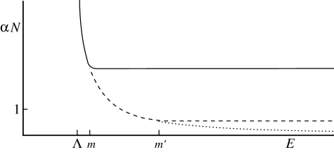
FIG. 1.: Running coupling in the ${\cal N}=1^{*}$ theory. For the solid curve the asymptotic $\alpha N$ is large and the decoupling scale $m$ is close to $\Lambda$. For the dashed curve the asymptotic $\alpha N$ is small and the decoupling scale is $m^{\prime}\gg\Lambda$. The asymptotically free ${\cal N}=1$ curve is dotted.

When $m\gg\Lambda$, the dual string coupling $g=\alpha$ is small but the space on which the strings propagate is highly curved, with curvature radius $R\sim(gN)^{1/4}$, so there is no weakly-coupled string description. Fortunately, in this case ordinary field theoretic perturbation theory works well for $\mu>\Lambda$, both below and above $\mu=m$. Conversely, in order that $gN$ be large (with $g$ small), so as to allow a weakly-coupled string description, the scale $m$ of the additional matter must be essentially the confinement scale $\Lambda$ where the mass gap is generated. In this case field theory perturbative techniques are not useful at any scale. By varying $g$ we can interpolate between these two cases.

The analysis in Sections II and III is field theoretic. In Section II we review DIS, including the definitions of the kinematic variables $q^{2}$ and $x$. We also review the operator product expansion (OPE) analysis, and apply it at small ’t Hooft coupling. Section III extends the OPE analysis to large ’t Hooft coupling.

The results are as follows. At small ’t Hooft coupling, where field theory perturbation theory applies, hadronic substructure is similar to that in QCD. Each hadron typically has a small number of partons carrying most of the energy, surrounded by a cloud of wee partons with very small momentum fraction $x$. At large ’t Hooft coupling, where the stringy dual description is perturbative, we find that hadronic substructure is qualitatively different. All the partons are wee; parton evolution is so rapid that the probability of finding a parton with a substantial fraction of the energy is vanishingly small. At finite $N$ each hadron has a diffuse cloud of other hadrons surrounding it. For most processes the incoming electron is most likely, as $q^{2}\to\infty$ with fixed $N$ and $x$, to scatter off one of the hadrons in the cloud. It is as though the electron could find no quarks at finite $x$ inside the proton, due to their fragmentation into huge numbers of quarks, antiquarks and gluons, and instead were more likely to strike the very diffuse pion cloud around the proton.

The transition from one behavior to the other is most likely continuous, and takes the following form: the traditional lowest-twist operators of QCD develop large anomalous dimensions and become high-twist operators as the ’t Hooft coupling becomes large. However, certain double-trace operators, normally subleading in QCD, do not get large anomalous dimensions; their twists remain relatively low. Consequently, these traditionally higher-twist operators begin to dominate deep-inelastic scattering as the ’t Hooft coupling grows large. From the string theory side, the transition is most easily understood beginning from large ’t Hooft coupling, when the background on which the string propagates is weakly curved. As the ’t Hooft coupling shrinks and the curvature radius of the background becomes small, the masses of stringy modes shrink relative to those of the Kaluza-Klein modes. When both modes have masses of the same order, a cross-over to new behavior occurs. This transition is the same one which connects the picture of D-branes, with open strings coupled to closed strings, to that of black holes, with only closed strings.

Sections IV and V present the string theoretic calculations of the DIS structure functions. In terms of calculational method we find that there are three distinct regimes of $x$: of order one, of order $(gN)^{-1/2}$, and of order $e^{-(gN)^{1/2}}$. Section IV deals with the first of these. In this regime excited strings are not produced, and so the calculation involves only supergravity degrees of freedom. The results are consistent with the earlier OPE analysis, and in addition give the detailed form of the structure functions. We discuss the qualitative form of the amplitudes, where the the warped spacetime geometry plays an important role, and we compare the inelastic results here to the results for the elastic amplitudes in Ref. [2].

To complete the analysis — in particular, to verify the energy-momentum sum rule — we must determine the amplitudes also at small $x$. This is done in Section V. In this case the scattering produces excited strings. We first analyze the amplitude assuming, as in Ref. [2], that the scattering process is localized and so can be approximated locally by the flat spacetime amplitude. The resulting structure functions give Regge behavior (consistent with a Pomeron-exchange picture) but with a divergent momentum sum rule. The effect that cuts this off is the logarithmic growth of strings at high energy [5]. When $x$ is exponentially small, the string size becomes comparable to the AdS radius and existing methods for perturbative string calculation break down. By using the world-sheet renormalization group we are able to include the effects of string growth. This sums all orders in $(gN)^{-1/2}\ln x$ and produces a result valid down to $x=0$.

Section VI presents conclusions and speculations.

We have learned that O. Andreev is also considering DIS in gauge/gravity duality. We also note the recent papers [6] on elastic scattering in the hard and Regge regimes.

II Deep Inelastic Scattering

Deep inelastic scattering — the scattering of electrons off of hadrons in kinematic regimes where the hadron is broken apart — is a natural probe of hadronic substructure. The electron plays no role except to emit an off-shell photon of four-momentum $q^{\mu}$; the photon then strikes the hadron, probing it near the lightcone at distances of order $1/\sqrt{q^{2}}$. As shown by Bjorken, if hadrons are made of essentially free massless partons which appear in the hadronic wave function with some distribution of momentum and energy, then this distribution can be measured. In particular, defining $x=-q^{2}/2P\cdot q$, where $P^{\mu}$ is the momentum of the scattered hadron, the probability of finding a parton with four-momentum $xP^{\mu}$ is a distribution function $f(x,q^{2})$ that is independent of $q^{2}$.

This $q^{2}$-independence, called Bjorken scaling, is a property only of the truly free parton model. In real QCD, scaling is of course violated; the parton distribution functions “evolve” as $q^{2}$ increases, because each parton, through QCD interactions, tends to split into multiple partons of smaller $x$. Consequently the apparent structure of a QCD hadron depends on $q^{2}$, with the number of partons increasing and their average $x$ decreasing as $q^{2}$ increases. This physical picture can be derived from a precise operator product analysis, which we now review.

A Review of general formalism

We will use the conventions and notations of Ref. [7], except that we take the metric $(-1,+1,+1,+1)$ to connect with standard string calculations. As explained in any standard treatment, the DIS amplitudes for electron-hadron scattering can be extracted from the imaginary part of forward Compton scattering, or more precisely from the matrix element of two electromagnetic currents inside the hadron of interest

$${\sf T}^{\mu\nu}\equiv i\int\ d^{4}y\,e^{iq\cdot y}\langle P,{\cal Q}|T(J^{\mu}(y)J^{\nu}(0))|P,{\cal Q}\rangle\ .$$ (1)

Here $T({\cal O}_{1},{\cal O}_{2})$ indicates a time-ordered product, $P^{\mu}$ is the momentum of the hadron, and ${\cal Q}$ is its electromagnetic charge. In complete generality this can be written

$${\sf T}_{\mu\nu}=\widetilde{F}_{1}\left(x,{q^{2}\over\Lambda^{2}}\right)\left(g_{\mu\nu}-{q_{\mu}q_{\nu}\over q^{2}}\right)+{2x\over q^{2}}\widetilde{F}_{2}\left(x,{q^{2}\over\Lambda^{2}}\right)\left(P_{\mu}+{q_{\mu}\over 2x}\right)\left(P_{\nu}+{q_{\nu}\over 2x}\right)\ .$$ (2)

Here

$$x=-q^{2}/2P\cdot q\ ,\quad q^{2}>0\ ,\quad 0\leq x\leq 1\ .$$ (3)

$\Lambda$ is a mass-scale in QCD — typically the hadron mass $M^{2}=-P^{2}$. Note that the structure functions $\widetilde{F}_{1}$ and $\widetilde{F}_{2}$ are dimensionless; in the parton model their imaginary parts are related to the parton distribution functions, as will be discussed below. These functions may be extracted from $g^{\mu\nu}{\sf T}_{\mu\nu}$ and $P^{\mu}P^{\nu}{\sf T}_{\mu\nu}$; note that $q^{\mu}{\sf T}_{\mu\nu}$ vanishes by current conservation.

In the unphysical region of $x\gg 1$, ${\sf T}^{\mu\nu}$ can be reexpressed using the operator product expansion (OPE) of the two currents. On general grounds [conservation of $J^{\mu}$ and Lorentz invariance, and dropping terms that would vanish in the diagonal matrix element (1),] the OPE takes the form

$$\int d^{4}y\ e^{iq\cdot y}\,T(J^{\mu}(y)J^{\nu}(0)) = \sum_{n=0,2,4,\dots}\sum_{j}{\cal O}_{n,j}^{\rho_{1}\ldots\rho_{n}}(0){q_{\rho_{3}}\ldots q_{\rho_{n}}\over q^{n+\delta_{n,j}}}\Biggl{(}\frac{\Lambda^{2}}{q^{2}}\Biggr{)}^{\gamma_{n,j}/2}$$ (6)

$$\qquad\Bigg{[}\left(q^{2}g_{\mu\nu}-{q_{\mu}q_{\nu}}\right){q_{\rho_{1}}q_{\rho_{2}}}C_{n,j}^{(1)}$$

$$\qquad\quad+\left(q^{2}g_{\mu\rho_{1}}-{q_{\mu}q_{\rho_{1}}}\right)\left(q^{2}g_{\nu\rho_{2}}-{q_{\nu}q_{\rho_{2}}}\right)C_{n,j}^{(2)}\ \Bigg{]}\ .$$

Here $n$ is the spin of the operator ${\cal O}_{n,j}$ and $j$ indexes the various operators of spin $n$; the engineering dimension of ${\cal O}_{n,j}$ is $\delta_{n,j}$ and $\gamma_{n,j}$ is its anomalous dimension. We also define $\Delta_{n,j}=\delta_{n,j}+\gamma_{n,j}$ as the total scaling dimension of ${\cal O}_{n,j}$ and $\tau_{n,j}=\Delta_{n,j}-n$ is its twist. For simplicity we have written this for the scale-invariant case, where the dimensions $\Delta_{n,j}$ are constant but in general noncanonical. In QCD the dimensions vary only logarithmically, through the running of the coupling, and the above expression can be used locally in $q^{2}$. The $C_{n,j}^{(s)}$ are dimensionless.

By Lorentz invariance, the (spin-averaged) matrix elements take the form

$$\langle P,{\cal Q}|{\cal O}_{n,j}^{\rho_{1}\cdots\rho_{n}}|P,{\cal Q}\rangle=\Lambda^{\delta_{n,j}-n-2}(-2)^{n}P^{\rho_{1}}\cdots P^{\rho_{n}}{A}_{n,j}+{\rm traces}\ ,$$ (7)

where ${A}_{n,j}$ is a pure number. The factors of $-2P^{\rho}$ combine with those of $q_{\rho}$ to give factors of $-2P\cdot q=q^{2}/x$, and so

$${\sf T}^{\mu\nu} \approx i\sum_{n\ {\rm even}}\sum_{j}x^{-n}\Biggl{(}{\Lambda^{2}\over q^{2}}\Biggr{)}^{{1\over 2}\tau_{n,j}-1}\$$ (9)

$$\qquad\left\{\Biggl{(}g_{\mu\nu}-{q_{\mu}q_{\nu}\over q^{2}}\Biggr{)}{A}_{n,j}C^{(1)}_{n,j}+{4x^{2}\over q^{2}}\biggl{(}P_{\mu}+{q_{\mu}\over 2x}\biggr{)}\biggl{(}P_{\nu}+{q_{\nu}\over 2x}\biggr{)}{A}_{n,j}C^{(2)}_{n,j}\right\}\ ,$$

where we have dropped the trace terms, which are suppressed by powers of $q^{2}$. Thus

$$\widetilde{F}_{s}(x,q^{2})\approx i\sum_{n\ {\rm even}}\sum_{j}C^{(s)}_{n,j}A_{n,j}\,x^{-n}(2x)^{s-1}\left({\Lambda^{2}\over q^{2}}\right)^{{1\over 2}\tau_{n,j}-1}\ \ \ (s=1,2)\ .$$ (10)

We see that the operators that dominate the amplitudes at large $q^{2}$ are those that have the smallest twist $\tau$. Note both ${C}_{n,j}^{(s)}$ and ${A}_{n,j}$ depend on the normalization of ${\cal O}_{n,j}$; however only the product ${C}_{n,j}^{(s)}{A}_{n,j}$ appears in the end.

The OPE determines the behavior in the limit that $q^{2}$ and $x$ are both large. The physical region for DIS is $0\leq x\leq 1$. A standard contour argument relates the behavior at large $x$ to the moments of the DIS structure functions. Integrate with respect to $\omega\equiv 1/x$ around a contour surrounding $\omega=0$

$${1\over 2\pi}\int_{|\omega|=\epsilon}d\omega\ \omega^{-n-1}(\omega/2)^{s-1}\widetilde{F}_{s}(\omega^{-1},q^{2})\approx{C^{(s)}_{n,j}A_{n,j}}\Biggl{(}{\Lambda^{2}\over q^{2}}\Biggr{)}^{{1\over 2}\tau_{n,j}-1}\ .$$ (11)

One now deforms the contour out to $|\omega|=\infty$, except along the real axis for $\omega>1$ and $\omega<-1$, where there are branch cuts. The optical theorem for the discontinuity across the branch cut then determines the moments

$$M^{(s)}_{n}(q^{2})\equiv\int_{0}^{1}dx\ x^{n-1}(2x)^{1-s}{F_{s}(x,q^{2})}\approx\frac{1}{4}\sum_{j}{C^{(s)}_{n,j}A_{n,j}}\left({\Lambda^{2}\over q^{2}}\right)^{{1\over 2}\tau_{n,j}-1}\ \ (n\ {\rm even},s=1,2)$$ (12)

where

$$F_{s}(x,q^{2})\equiv 2\pi\,{\rm Im}\,\widetilde{F}_{s}(x,q^{2})\ .$$ (13)

These structure functions are the standard ones appearing in the hadronic tensor

$${\sf W}^{\mu\nu}\equiv i\int\ d^{4}y\,e^{iq\cdot y}\langle P,{\cal Q}|[J^{\mu}(y),J^{\nu}(0)]|P,{\cal Q}\rangle\ .$$ (14)

The second term in the commutator vanishes, and the first, with a complete set of states inserted between the currents, gives the square of the DIS amplitude. The functions $F_{s}$ are defined by

$${\sf W}_{\mu\nu}=F_{1}\left(x,{q^{2}\over\Lambda^{2}}\right)\left(g_{\mu\nu}-{q_{\mu}q_{\nu}\over q^{2}}\right)+{2x\over q^{2}}F_{2}\left(x,{q^{2}\over\Lambda^{2}}\right)\left(P_{\mu}+{q_{\mu}\over 2x}\right)\left(P_{\nu}+{q_{\nu}\over 2x}\right)\ .$$ (15)

B Specializing to weak coupling

In a free parton model (QCD or Yang-Mills at zero coupling) it is easy to see that the only operators that appear in the $JJ$ OPE have $\tau=2,4,6,\ldots$. In a theory with adjoint fields only, each operator involves a certain number of traces over color indices. The leading multi-trace operators have $\tau\geq 4$, so DIS is dominated by a set of single-trace twist-2 operators ${\cal T}_{n,j}$, with classical dimension $n+2$ and spin $n$. These include the energy-momentum tensor.

For finite coupling, the ${\cal T}_{n,j}$ develop anomalous dimensions $\gamma_{n,j}$ (which are positive) except for the energy-momentum tensor whose conservation always implies $\gamma=0$. Of course, in leading-order perturbation theory the anomalous dimensions $\gamma_{n,j}\sim\alpha N$ ($N$ is the number of colors and $\alpha$ is the coupling at the scale $q^{2}$) so in an asymptotically-free theory such as QCD or Yang-Mills, the ${\cal T}_{n,j}$ have twist close to 2 at high $q^{2}$ and are the lowest-twist operators appearing in the OPE.

For theories weakly coupled in the UV, the moments are then

$$M^{(s)}_{n}(q^{2})\approx\frac{1}{4}{\sum_{j}}^{\prime}{C^{(s)}_{n,j}A_{n,j}}\left({\Lambda^{2}\over q^{2}}\right)^{{1\over 2}\tau_{n,j}-1}\ \approx\frac{1}{4}{\sum_{j}}^{\prime}{C^{(s)}_{n,j}A_{n,j}}\left({\Lambda^{2}\over q^{2}}\right)^{{1\over 2}\gamma_{n,j}}\ \ \ (n\ {\rm even},s=1,2)\ ,$$ (16)

where the prime on the sum indicates that we keep only the terms corresponding to the ${\cal T}_{n,j}$; other terms are suppressed by powers of $q^{2}$. The $\gamma_{n,j}$ are positive, so the $M_{n}$ decrease to zero as $q^{2}$ increases. The exception is $n=2$: the energy-momentum tensor has no anomalous dimension and therefore gives $q^{2}$-independent sum rules

$$M_{2}^{(1)}(q^{2}) \equiv \int_{0}^{1}dx\,x\,F_{1}(x,q^{2})\ {\to}\ {\rm constant}\ ,$$ (17)

$$M_{2}^{(2)}(q^{2}) \equiv {1\over 2}\int_{0}^{1}dx\,F_{2}(x,q^{2})\ \to\ {\rm constant}\ ,$$ (18)

as $q^{2}\to\infty$. In general, however,

$$M_{n}^{(s)}\propto\left({\Lambda^{2}\over q^{2}}\right)^{{1\over 2}\tau_{n,j}-1},\quad\tau_{n}\equiv\min_{j}{\tau_{n,j}}$$ (19)

at large $q^{2}$. The fact that the moments vary as powers of $q^{2}$ in a conformal field theory was noted in ref. [8]; we will therefore call this power-law violation of Bjorken scaling Kogut-Susskind evolution.

C Parton interpretation of leading-twist effects

In a parton model, one interprets ${\sf W}^{\mu\nu}$ in terms of distributions of partons inside the hadron. If the partons have spin-${1\over 2}$ one finds that $F_{2}=2xF_{1}$ (the Callan-Gross relation) and that

$$F_{1}(x,q^{2})={1\over 2}\sum_{i}{\cal Q}_{i}^{2}f_{i}(x)\ .$$ (20)

Here $f_{i}$ is the parton distribution function of parton-type $i$, which has charge ${\cal Q}_{i}$. Thus both $F_{1}$ and $F_{2}$ are $q^{2}$-independent in the parton model; this is Bjorken scaling.

Since in real QCD the anomalous dimensions of the ${\cal T}_{n,j}$ are not zero, the functions $F_{1}$ and $F_{2}$ evolve with $q^{2}$. This is expressed through the DGLAP equations [9], which may be written

$$q^{2}{dM_{n}\over dq^{2}}=-{1\over 2}\gamma_{n}M_{n}$$ (21)

in the simple case where there is only one ${\cal T}_{n,j}$ for each $n$. This is understood conceptually as evolution of the parton distribution functions with $q^{2}$, through the relation between the $F_{s}$ and the $f_{i}$. In leading-order perturbation theory the $\gamma_{n}$ are simply the moments of the parton splitting functions (times a factor of $\alpha_{s}$). The positivity of the $\gamma_{n}$ ensures that evolution acts to decrease the energy-fraction $x$ of the average parton, as one would expect on general physical grounds: as $q^{2}$ increases, the functions $f_{i}(x,q^{2})$ tend to shrink at larger $x$ and grow at small $x$. This is of course observed experimentally in QCD.

The energy-momentum sum rule from $M_{2}$,

$$M_{2}=\frac{1}{2}\int_{0}^{1}dx\ \sum_{i}x{\cal Q}_{i}^{2}f_{i}(x,q^{2})\to{\rm constant}$$ (22)

simply states in the parton model that the total charge-weighted energy of all partons does not change as one probes the system at increasingly short distances.

III Strong coupling: field theory analysis

A The OPE at large ’t Hooft coupling

Let us now apply this formalism to deep-inelastic scattering in four-dimensional confining theories in which the ’t Hooft coupling $gN$ can be varied between large and small values, and which are in either case nearly conformal above the confinement scale as in Fig. 1. We will assume that the theory has a symmetry current whose associated charge is carried by light degrees of freedom which are present inside hadrons (we will consider $U(1)$ currents, but again nonabelian currents or the energy momentum tensor could also be used). We can then study the current-current matrix element, Eq. (1), in the hadron of interest. Note that the hadrons might only be dipoles under this $U(1)$; for example, baryon number in QCD is not carried by any meson but a photon coupling to baryon number will still scatter off partons inside the meson.

We saw above that a generic theory at small $gN$ has DIS physics similar to that of QCD. At large $q^{2}$, hadrons can be treated as bound states of weakly-interacting partons with accompanying distribution functions. Since the anomalous dimensions of all single-trace operators are of order $gN$, the $\tau\approx 2$ operators ${\cal T}_{n,j}$ dominate the physics. The moments $M_{n}$ of the functions $F_{1}$ and $F_{2}/2x$ vary slowly, and Bjorken scaling is only weakly violated.

However, at large $gN$, the physics is totally different. One learns from AdS/CFT duality [1, 10] that the operators ${\cal T}_{n,j}$ (excepting the energy-momentum tensor) have large anomalous dimensions. These operators are related to states in the IIB string spectrum, and their dimensions (and consequently their anomalous dimensions and their twists) are of order

$$\Delta\sim\tau\sim\gamma\sim(gN)^{1/4}\gg 1\ .$$ (23)

So large are these anomalous dimensions that (excepting $T^{\mu\nu}$) the ${\cal T}_{n,j}$ are no longer the leading-twist operators. On general grounds, there are double-trace operators which do not receive large anomalous dimensions for any $gN$. It is these operators which dominate the OPE and are lowest-twist at large $gN$.

What are these double-trace operators? First, note that any theory, supersymmetric or not, has single-trace operators whose anomalous dimensions are order 1 even at large $gN$. Let us call these operators protected and refer to them as ${\cal P}_{p}$ (with dimension $\Delta_{p}$, spin $n_{p}$, twist $\tau_{p}=\Delta_{p}-n_{p},$ and charge ${\cal Q}_{p}$ under the $U(1)$ symmetry) where the index $p$ simply labels the operators. The energy-momentum tensor is such an operator; so are conserved currents; in supersymmetric theories other examples would include, but are not restricted to [21], the chiral operators.

Now we may construct double-trace operators, as bilinears in the ${\cal P}_{p}$, which can appear in the $JJ$ OPE. For simplicity, let us consider a spin-zero operator ${\cal P}_{p}$, and consider its bilinears, of the form ${\cal P}_{p}^{\dagger}{\cal P}_{p}^{\vphantom{\dagger}}$, ${\cal P}_{p}^{\dagger}\partial_{\mu}\partial_{\nu}{\cal P}_{p}^{\vphantom{\dagger}}$, and so on. Large-$N$ factorization as $N\to\infty$ implies that

$$\left\langle{{\cal P}_{p}^{\dagger}{\cal P}_{p}^{\vphantom{\dagger}}(y)\,{\cal P}_{p}^{\dagger}{\cal P}_{p}^{\vphantom{\dagger}}(0)}\right\rangle=\left|\left\langle{{\cal P}_{p}^{\vphantom{\dagger}}(y)\,{\cal P}_{p}^{\dagger}(0)}\right\rangle\right|^{2}+O\left({1\over N^{2}}\right)\ \sim r^{-4\Delta_{p}\pm{\rm order}\left(1/N^{2}\right)}\ ,$$ (24)

and thus the twist of ${\cal P}^{\dagger}{\cal P}$ is (at least) twice that of ${\cal P}$, up to a correction of order $1/N^{2}$. Similar arguments imply that the operators ${\cal P}^{\dagger}\partial_{\rho_{1}}\partial_{\rho_{2}}\cdots\partial_{\rho_{r}}{\cal P}$ have $\Delta=r+2\Delta_{p}$ and $\tau\geq 2\tau_{p}$, up to an ${\rm order}\left(\pm{1/N^{2}}\right)$ correction. When all Lorentz indices are symmetrized, with traces removed, to make an operator of maximum spin, the twist takes the minimum value $\tau\approx 2\tau_{p}$. Since ${\cal P}_{p}$ is protected, $\Delta_{p}$, and consequently $\tau_{p}$, has a finite limit as $gN\to\infty$. Altogether we conclude these double-trace operators have finite $\tau$ as $gN\to\infty$, and thus have smaller twist than any ${\cal T}_{n,j}$ at large $gN$.

This is by no means the complete set of double-trace operators which may appear in the OPE. We may also build them from ${\cal P}_{p}$ of non-zero spin, in which case index contractions are more complex. Furthermore, if ${\cal P}_{p}$ and ${\cal P}_{p^{\prime}}$ have the same global charges, then operators such as ${\cal P}_{p}^{\dagger}\partial_{\mu}\partial_{\nu}{\cal P}_{p^{\prime}}$ may appear. Although these operators are not subleading to the ones mentioned above, and must be included in all applications, we will omit them in our formulas in order to keep our presentation simple.

The essential point of this discussion is that these operators behave differently at large $gN$ from the unprotected operators ${\cal T}_{n,j}$. While the single-trace operators ${\cal T}_{n,j}$ have anomalous dimensions of order $gN$ in perturbation theory, and of order $(gN)^{1/4}\to\infty$ for $gN\to\infty$, a double-trace operator constructed from protected single-trace operators is itself protected: its anomalous dimension is largely inherited from its constituent single-trace operators, up to a shift of order $g/N$ in perturbation theory and of order $N^{-2}h(gN)$ for any $gN$. The function $h(gN)$ can in principle be computed for small and for large $gN$.

When we include both the ${\cal T}_{n,j}$ and the ${\cal P}_{p}^{\dagger}\partial\partial\cdots\partial{\cal P}_{p}$ from the OPE, the moments (16) become

$$M^{(s)}_{n}(q^{2})\approx\frac{1}{4}{\sum_{j}}^{\prime}{C^{(s)}_{n,j}A_{n,j}}\left({\Lambda^{2}\over q^{2}}\right)^{{1\over 2}\tau_{n,j}-1}\ +\frac{1}{4}{\sum_{p}}^{\prime\prime}{C^{(s)}_{n,p}A_{n,p}}\left({\Lambda^{2}\over q^{2}}\right)^{\tau_{p}-1}\ ,$$ (25)

where the primed sum runs over the ${\cal T}_{n,j}$ and the double-primed sum over the protected double-trace operators with spin $n$ and dimension $\approx 2\tau_{p}+n$.

For small $gN$, $\tau_{n,j}\sim 2+{\rm order}{(gN)}<2\tau_{p}$; for large $gN$, $\tau_{n,j}\sim(gN)^{1/4}$ but $\tau_{p}$ remains finite and order 1. Therefore, the first term dominates as $q^{2}\to\infty$ for small $gN$ while the last term dominates for large $gN$. Thus there is a qualitative transition at $gN\sim 1$ in which double-trace operators become the lowest-twist operators in the theory, aside from the energy-momentum tensor which remains twist-two.

Before interpreting this transition physically, we do the $N$ counting for the different contributions to the moments. The leading planar amplitude is of order $N^{2}$, and we normalize the currents and other single-trace operators such that they create hadrons at order $N^{0}$, and so have two-point functions of order $N^{0}$. (Note that with this normalization the partons have charges of order $N^{-1}$; our $U(1)$ currents must be multiplied by a factor of $N$ to give the usual normalization for the $R$-currents of ${\cal N}=1^{*}$ and similar theories.) Then for the OPE coefficients we have

$$C_{n,j}^{(s)}\propto\left\langle{J\ J\ {\cal T}_{n,j}}\right\rangle\sim{N^{-1}}\ ;\quad C_{n,p}^{(s)}\propto\left\langle{J\ J\ {\cal P}_{p}^{\dagger}(\partial)^{r}{\cal P}_{p}}\right\rangle\sim{N^{-2}}\ .$$ (26)

For the matrix elements

$$A_{n,j}=\langle{\cal Q},P|{\cal T}_{n,j}|{\cal Q},P\rangle\sim N^{-1}\ ;$$ (27)

$$A_{n,p}=\langle{\cal Q},P|{\cal P}_{p}^{\dagger}(\partial)^{r}{\cal P}^{\vphantom{\dagger}}_{p}|{\cal Q},P\rangle\sim{N^{0}}{\rm\ if}\ \langle{\cal Q},P|{\cal P}^{\vphantom{\dagger}}_{p}|0\rangle\neq 0\ ;$$ (28)

$$A_{n,p}=\langle{\cal Q},P|{\cal P}_{p}^{\dagger}(\partial)^{r}{\cal P}^{\vphantom{\dagger}}_{p}|{\cal Q},P\rangle\sim{N^{-2}}{\rm\ if}\ \langle{\cal Q},P|{\cal P}^{\vphantom{\dagger}}_{p}|0\rangle=0\ .$$ (29)

The last two equations follow from the fact that the matrix element is dominated by a (dis)connected graph if $\langle{\cal Q},P|{\cal P}_{p}|0\rangle$ is (non)zero.

Thus, from Eq. (27)–(29), almost all of the matrix elements $A_{n,p}$ appearing in the second sum in (25) are of order $1/N^{2}$. Only for those ${\cal P}_{p}$ that have charge ${\cal Q}$ are the elements (potentially) of order 1. Let us therefore write $A_{n,p}=a_{n,p}/N^{2}$ for those ${\cal P}_{p}$ with ${\cal Q}_{p}\neq{\cal Q}$, and separate the operators by charge:

$$M^{(s)}_{n}(q^{2}) \approx \frac{1}{4}{\sum_{j}}^{\prime}{C^{(s)}_{n,j}A_{n,j}}\left({\Lambda^{2}\over q^{2}}\right)^{{1\over 2}\tau_{n,j}-1}\ +\frac{1}{4}{\sum_{{\cal Q}_{p}={\cal Q}}}^{\prime\prime}{C^{(s)}_{n,p}A_{n,p}}\left({\Lambda^{2}\over q^{2}}\right)^{\tau_{p}-1}$$ (31)

$$\qquad+{1\over 4N^{2}}{\sum_{{\cal Q}_{p}\neq{\cal Q}}}^{\prime\prime}{C^{(s)}_{n,p}a_{n,p}}\left({\Lambda^{2}\over q^{2}}\right)^{\tau_{p}-1}\ .$$

From this we see that while the first term dominates at small $gN$, the situation at large $gN$ is more complex. At $q^{2}$ somewhat larger than $\Lambda^{2}$ the second term always dominates; but it falls as $(q^{2})^{-\tau_{\cal Q}+1}$, where $\tau_{\cal Q}$ is the minimum twist of the operators ${\cal P}_{p}$ of charge ${\cal Q}$. Typically $\tau_{\cal Q}\sim{\cal Q}$; for example, if all fields carry electric charge 0 or 1, this will be the case. If $\tau_{\cal Q}\neq\tau_{\rm c}$ (where $\tau_{\rm c}$ is the minimum twist of all electrically charged operators ${\cal P}_{p}$) then there is yet another transition. When $q^{2}\gtrsim\Lambda^{2}N^{2/(\tau_{\cal Q}-\tau_{\rm c})}$, the third term becomes the largest of the three: the contribution of the operator ${\cal P}_{p}$ with lowest twist ($\tau_{p}=\tau_{\rm c}$) falls only as $(q^{2})^{-\tau_{\rm c}+1}$, and thus overcomes its overall $1/N^{2}$ suppression to dominate the amplitude as $q^{2}\to-\infty$.

FIG. 2.: Forward Compton amplitude in the parton model.

B Interpretation of the various contributions

Now we turn to the interpretation of this transition. The essential point is that the operators ${\cal T}_{n,j}$ are associated with partons, while the ${\cal P}_{p}^{\dagger}(\partial)^{r}{\cal P}^{\vphantom{\dagger}}_{p}$ are associated with hadrons. The local operators ${\cal T}_{n,j}$ couple to the internal constituents of hadrons (in QCD they are bilinear in quarks), while at large $N$ the operator ${\cal P}_{p}^{\dagger}(\partial)^{r}{\cal P}^{\vphantom{\dagger}}_{p}$ destroys and creates a whole hadron, and so is like a bilinear in hadron fields.

Let us first address the large anomalous dimensions of the ${\cal T}_{n,j}$. Consider the DGLAP equations (21), combined with the parton model expression (20) and the fact that anomalous dimensions $\gamma_{n}$ are proportional to the moments of the parton splitting amplitudes. From these we see that the $\gamma_{n,j}$ controls the rate of parton splitting. That $\gamma_{n,j}\gg 1$ at large $gN$ implies that parton-splitting processes, and consequent evolution of the parton distribution functions, are vastly more rapid at large $gN$. The contributions of ${\cal T}_{n,j}$ to the moments $M_{n}^{(s)}$ ($n>2$) decrease rapidly as the partons in the hadron split repeatedly, leaving parton distribution functions which only have support at very small $x$ (just how small, we will investigate in section V). This behavior explains why the first term in Eq. (31) is so suppressed at large $gN$.

FIG. 3.: Forward Compton amplitude with parton evolution; the parton splits, losing some fraction of its energy, before being struck by the photon.

FIG. 4.: As $gN$ increases the splitting rate increases as well; a large fraction of the parton’s energy is lost before it is struck.

Once the partons have fragmented into tiny pieces, what remains to dominate the moments $M_{n}^{(s)}$? If the currents cannot scatter off of partons, then perhaps they can scatter off of entire hadrons. Unlike partons, which carry color and radiate strongly at large $gN$, colorless hadrons are much less likely to lose their energy through radiation. In fact, at $N\to\infty$, for any $gN$, they cannot do so at all. In this limit, the only thing which can happen at moderate values of $x$ is that the currents can scatter off the entire parent hadron $|{\cal Q},P\rangle$. One might naively expect that this contribution would have support only at $x=1$. However, as we will calculate shortly, this is not so, because the scattering need not be elastic even though individual partons are not struck. Instead the currents can coherently excite the internal structure of the hadron, without breaking it.

FIG. 5.: The photon may instead strike the entire hadron coherently. While suppressed relative to the parton model diagram, it is not as suppressed as the diagram at large $gN$.

Still, for the currents to strike the hadron in this way requires that the entire hadron shrink down to a size of order $q^{-1}$, a fluctuation which has amplitude proportional to $q^{-(\Delta-1)}$, where $\Delta$ is the dimension of the lowest-dimension operator which can create this hadron. More precisely, when spin and associated momentum factors are accounted for, the suppression factor becomes $q^{-(\tau-1)}$, where $\tau$ is the twist of the lowest-twist operator which can create the hadron. (A similar factor governs scattering amplitudes at large angles [2]). Since all such operators have charge ${\cal Q}$, the dominant contribution to Eq. (31) of this type should scale as $(q^{2})^{-(\tau_{\cal Q}-1)}$, where $\tau_{\cal Q}$ is the minimum twist of operators in the theory with charge ${\cal Q}$. Indeed, the second term in Eq. (31) has this form.

At finite $N$, hadrons are interacting, and therefore hadron number is not conserved. Any low-lying eigenstate of the Hamiltonian is an admixture of a single hadron with a small admixture (of order $1/N^{k-1}$) of a $k$-hadron state. More physically, the parent hadron surrounds itself with a diffuse cloud of other hadrons, some of them uncharged but some charged. What is the probability that the currents will strike not the parent hadron but an electrically charged hadron in the cloud? Clearly it must vanish as $N\to\infty$; but the momentum suppression factor for this process is $(q^{2})^{-(\tau_{\rm c}-1)}$, where $\tau_{\rm c}$ is the lowest-twist operator which can create a charged object in the cloud. The cloud-scattering contribution will be much less suppressed at large $q^{2}$ than the parent-scattering, unless $\tau_{\cal Q}=\tau_{\rm c}$. The third term in Eq. (31), then, represents scattering of the current off the diffuse cloud surrounding the parent hadron. The product $C_{n,p}^{(s)}a_{n,p}$ is related, in analogy to the parton case, to a hadron distribution function in the cloud.

FIG. 6.: The parent hadron has a cloud of smaller hadrons which surrounds it. At very large $q^{2}$ the photon is most likely to strike the smaller hadron.

IV Strong coupling: string theory analysis

A Introduction

At large ’t Hooft parameter, the gauge theories of interest have a dual string description, in which we can calculate the functions $F_{1,2}$ directly. In this section we carry out this calculation, verifying the conclusions of the OPE analysis as well as obtaining more detailed information about the $x$-dependence.

For conformal gauge theories, the dual string theory lives in a space $AdS_{5}\times W$, where $W$ is $S^{5}$ or other Einstein space. The metric is

$$ds^{2}=\frac{r^{2}}{R^{2}}\eta_{\mu\nu}dy^{\mu}dy^{\nu}+\frac{R^{2}}{r^{2}}dr^{2}+R^{2}\widehat{ds}_{W}^{2}\ ,$$ (32)

where $R=(4\pi gN)^{1/4}\alpha^{\prime 1/2}$ is the AdS radius. The four coordinates $y^{\mu}$ are identified with those of the gauge theory, while $r$ is the holographic radial coordinate; coordinates on $W$ will be denoted $\Omega$. The key feature of this geometry is the gravitational redshift (warp factor) multiplying the four-dimensional flat metric. The conserved momenta, which are identified with those of the gauge theory, are $p_{\mu}=-i\partial_{\mu}$. The momenta as seen by a local local inertial observer in ten dimensions are

$$\tilde{p}_{\mu}=\frac{R}{r}p_{\mu}\ .$$ (33)

The characteristic energy scale in ten dimensions is $R^{-1}$ (up to powers of the dimensionless ’t Hooft coupling), so the characteristic four-dimensional energy is

$$E\sim\frac{r}{R^{2}}\ .$$ (34)

Thus, four-dimensional energies depend on the five-dimensional position, going to zero at the horizon $r=0$, and diverging at the AdS boundary $r=\infty$.

In confining theories, the geometry is approximately of the above form at large $r$, but is modified at radii corresponding to the gauge theory mass gap,

$$r\sim r_{0}=\Lambda R^{2}\ ,$$ (35)

so that the warp factor no longer goes to zero. The details of the small-radius geometry, and the form of the space $W$, depend on the precise gauge theory and on the mechanism by which conformal invariance is broken. However, the dynamics of interest for large $q^{2}$ takes place at $r\gg r_{0}$ where the conformal metric (32) holds, and does not depend on the detailed form of $W$.

Qualitatively, such a theory is similar to QCD, which also has (nearly) conformal physics in the ultraviolet, and exhibits confinement and a mass gap in the infrared. In QCD the ultraviolet is nearly Gaussian, and one sees approximate Bjorken scaling, but any theory in this class will be expected to exhibit approximate Kogut-Susskind evolution, which includes Bjorken scaling as a special case.

We will imagine that we are considering a theory with a $U(1)$ symmetry current, whose associated charge is carried by light degrees of freedom which are present inside hadrons. We can then study the current-current matrix element, Eq. (1), in the hadron of interest, and extract from that computation the same information about hadronic structure functions that would be obtained by deep inelastic scattering via a photon coupled to the $U(1)$ current.

B Examples

The calculation is largely independent of the details of the gauge theory, but for completeness we briefly discuss some examples of theories in which this physics can be concretely studied. This section lies outside the mainstream of the paper and may be skipped.

The simplest way to break conformal invariance is to begin with the ${\cal N}=4$ theory and add ${\cal N}=1$ supersymmetric mass terms for all superfields except a single ${\cal N}=1$ vector multiplet. According to the AdS/CFT dictionary [10], this ‘${\cal N}=1$^∗’ theory corresponds to deforming the string theory on $AdS_{5}\times S^{5}$ by a nonnormalizable three-form flux at the boundary. This flux is a perturbation in the conformal regime but its effect becomes large at small radius. The resulting geometry was found in ref. [4]. One or more expanded five-branes appear near $r_{0}$, depending on the gauge theory phase; in the confining phase there is a single NS5-brane. One can also add mass terms to break the supersymmetry completely, but the regime of stability of the resulting theories has not been precisely determined.

In cascading theories, the transverse space $W=T^{1,1}$ is topologically $S^{3}\times S^{2}$ with appropriate three-form fluxes. The ${\cal N}=1$ gauge theory, $SU(N+M)\times SU(N)$ with bifundamentals, cascades down to pure ${\cal N}=1$ $SU(M)$ (in the simplest case where $M$ divides $N$), which confines. The corresponding geometry is smoothly cut off at small $r$ [12]. In this case the geometry is not precisely conformal at large $r$, but evolves logarithmically due to the cascade; we will ignore this slow evolution.

In both of these examples there are continuous symmetries of $W$, respectively $SO(3)$ and $SU(2)\times SU(2)$, which correspond to global symmetries of the gauge theory. We will consider DIS via the corresponding currents. We should point out that neither of these examples exhibits the transition in the precise form discussed in the previous section, for the simple reason that in the limit of small $gN$ everything decouples except for a pure ${\cal N}=1$ gauge theory which has no continuous global symmetries — all fields transforming under the global symmetries of $W$ have masses that are exponentially large compared to the confinement scale. However, this is not relevant, for several reasons. First, our present concern is only to make contact with the previous discussion of large $gN$, not to follow the transition to small $gN$. Second, it does not mean that the transition does not occur — it means only that there are no spin-one currents we can use to observe it. One should remember that there is nothing sacred in spin-one currents (unless one assigns religious significance to light, for which, admittedly, there is precedent) and our extended discussion of such currents reflects the specific fact that in nature we have no other option for probing QCD. At a purely theoretical level, we can imagine using spin-2 gravitons, corresponding to the operator product $T_{\mu\nu}T_{\sigma\rho}$; the earlier analysis generalizes directly and this gravitational DIS exhibits the transition. Third, there are various generalizations that would give weakly coupled theories with nontrivial global symmetries: keeping one of the masses zero in ${\cal N}=1$^∗ theory; orbifolding the ${\cal N}=1$^∗ theory [4]; adding whole D3-branes to the cascading theories; or, adding D7-branes to either theory. In each of these examples the details of the decoupling are somewhat intricate, and we will not go into this subject here.

C Computation at finite $x$

We will now use the dual string theory to calculate the matrix element

$${\sf T}^{\mu\nu}=i\langle P,{\cal Q}|T(\tilde{J}^{\mu}(q)J^{\nu}(0))|P,{\cal Q}\rangle\ ,$$ (36)

(where $\tilde{J}^{\mu}$ denotes the Fourier transform), or at least its imaginary part

$${\rm Im}\,{\sf T}^{\mu\nu} = \pi\sum_{{P}_{X},X}\langle P,{\cal Q}|J^{\nu}(0)|P_{X},X\rangle\,\langle P_{X},X|\tilde{J}^{\mu}(q)|P,{\cal Q}\rangle$$ (37)

$$= 2\pi^{2}\sum_{X}\delta(M_{X}^{2}+[P{+}q]^{2})\,\langle P,{\cal Q}|J^{\nu}(0)|P{+}q,X\rangle\,\langle P{+}q,X|J^{\mu}(0)|P,{\cal Q}\rangle\ ,$$ (38)

which is what appears in DIS.

We will use indices $M,N,\ldots$ to denote all ten spacetime dimensions, separating into $m,n,\ldots$ on $AdS_{5}$ and $a,b,\ldots$ on $W$; the former separate further into $(\mu,r)$. We must be a bit careful to distinguish the flat four-dimensional metric from the warped ten-dimensional metric. The momenta $P_{\mu}$, $q_{\mu}$, the polarization $n_{\mu}$, and the currents $J_{\mu}$ will be regarded as four-dimensional quantities and will be raised or contracted with $\eta^{\mu\nu}$. Indices $M,N,\ldots$, $m,n,\ldots$, and $a,b,\ldots$ will be raised or contracted with the ten-dimensional metric. An invariant written without a tilde refers to the four-dimensional gauge theory kinematics, e.g. $t=-q^{2}=-\eta^{\mu\nu}q_{\mu}q_{\nu}$. An invariant with a tilde, e.g. $\tilde{t}$, refers to the kinematics in the ten-dimensional metric.

The initial/final hadron is dual to a string state with wavefunction

$$\Phi=e^{iP\cdot y}\psi(r,\Omega)$$ (39)

in ten dimensions. The function $\psi(r,\Omega)$ is a normalizable mode [10] in the cut-off $AdS_{5}\times W$ space, like a cavity mode in a box. For a given hadron this function will be an eigenstate of the appropriate Laplacian. Different eigenfunctions correspond from the four-dimensional point of view to different hadrons, so that the full hadron spectrum is given by summing over the different string states and over the different radial Kaluza-Klein (KK) modes of each. (The term “radial KK modes” refers to four-dimensional modes reduced both on $W$ and the $AdS$-radial direction; for five-dimensional modes reduced on $W$ only, we will use simply “KK modes”.) We will take the initial and final hadron to be unexcited strings, massless in ten dimensions, and for simplicity will focus on the spinless dilaton. The currents correspond to perturbations of the boundary conditions at $r=\infty$, which excite nonnormalizable modes in the bulk [10]. Schematically, the calculation is then as shown in Fig. 2.

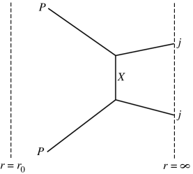
FIG. 7.: AdS/CFT prescription for ${\sf T}^{\mu\nu}$. The modification of AdS space at small radius is shown schematically as a sharp cutoff.

For reasons that will soon become apparent, the bulk interaction occurs in the large-radius region, $r\gg r_{0}$, where the spacetime is essentially a product $AdS_{5}\times W$. The current that couples to the hadron corresponds to an isometry of $W$, with Killing vector $v_{a}$. It excites a nonnormalizable mode of a Kaluza-Klein gauge field,

$$\delta g_{ma}=A_{m}(y,r)v_{a}(\Omega)\ .$$ (40)

The boundary limit of $A_{\mu}$ is the external potential in the gauge theory:

$$\lim_{r\to\infty}A_{\mu}(y,r)=A_{\mu}(y)|_{\rm 4d}\ .$$ (41)

There is no normalization factor to worry about: a state of unit charge in the gauge theory maps to a state of unit charge in the bulk. A nonnormalizable perturbation with boundary condition

$$A_{\mu}(y,\infty)=n_{\mu}e^{iq\cdot y}$$ (42)

then corresponds to the operator insertion $n_{\mu}\tilde{J}^{\mu}(q)$. The gauge field satisfies Maxwell’s equation in the bulk, $D_{m}F^{mn}=0$. It is convenient to work in the Lorenz-like gauge

$$i\eta^{\mu\nu}q_{\mu}A_{\nu}+R^{-4}r\partial_{r}(r^{3}A_{r})=0\ .$$ (43)

The field equations are then

$$-q^{2}A_{\mu}+R^{-4}r\partial_{r}(r^{3}\partial_{r}A_{\mu}) = 0\ ,$$ (44)

$$-q^{2}A_{r}+R^{-4}\partial_{r}\{r\partial_{r}(r^{3}A_{r})\} = 0\ .$$ (45)

The solution, with the given boundary and gauge conditions, is

$$A_{\mu} = n_{\mu}e^{iq\cdot y}\frac{qR^{2}}{r}K_{1}(qR^{2}/r)\ ,$$ (46)

$$A_{r} = iq\cdot ne^{iq\cdot y}\frac{R^{4}}{r^{3}}K_{0}(qR^{2}/r)\ .$$ (47)

(where by $q$ alone we mean $\sqrt{q^{2}}$).

Note that the potential falls off rapidly at $r<qR^{2}$, from the exponential behavior of the Bessel functions: the further $q$ is from the mass shell, the less the perturbation propagates into the AdS interior. We are interested in hard scattering, $q\gg\Lambda$, and so the interaction must occur in the large-$r$ conformal region,

$$r_{\rm int}\sim qR^{2}\gg r_{0}=\Lambda R^{2}\ .$$ (48)

We can then use the leading behavior for the wavefunction of the initial and final hadron, as in Ref. [4],

$$\Phi_{\rm i}=\Phi_{\rm f}^{*}\equiv\langle 0|\Phi|P,{\cal Q}\rangle\sim e^{iP\cdot y}f(r)Y(\Omega)\ ,\quad f(r)\propto r^{-\Delta}\ .$$ (49)

In a conformal theory, the mass eigenstates would be of this precise form, with $\Delta$ the conformal dimension of the state, which is also the dimension of the local operator ${\cal P}$ that creates the state from vacuum. In our case, the nonconformal dynamics at small $r$ causes a mixing between such terms, and the term with smallest $\Delta$ dominates at large $r$. The normalization of this state was explained in the appendix to Ref. [4]: for a canonically normalized scalar field, canonical quantization gives

$$\int dr\,d^{5}\Omega\,e^{2A}\sqrt{g_{\perp}}\,|\psi(r,\Omega)|^{2}=1\ ,$$ (50)

where

$$ds^{2}=e^{2A(r,\Omega)}\eta_{\mu\nu}dy^{\mu}dy^{\nu}+ds^{2}_{\perp}\ .$$ (51)

The normalization integral is dominated by the IR region $r\sim r_{0}$, where $e^{2A}\sqrt{g_{\perp}}\sim r_{0}R^{4}$. It follows that $\psi(r_{0},\Omega)\sim 1/R^{2}r_{0}$ and

$$f(r)=\frac{c_{\rm i}}{R^{4}\Lambda}(r/r_{0})^{-\Delta}$$ (52)

with $c_{\rm i}$ a dimensionless constant. We have defined the angular wavefunction to have the dimensionless normalization

$$\int d^{5}\Omega\,\sqrt{\hat{g}_{W}}\,|Y(\Omega)|^{2}=1\ ,$$ (53)

where $(\hat{g}_{W})_{ab}$ is the dimensionless metric as defined in (32). The details of conformal symmetry breaking enter only through the value of $c_{\rm i}$.

Now let us consider the nature of the intermediate state $X$. Since we are working in the leading large-$N$ approximation, only single-hadron (= single-string) states will contribute. The important issue is whether these are massless or excited strings. In the gauge theory,

$$s=-(P+q)^{2}=q^{2}\biggl{(}\frac{1}{x}-1\biggr{)}\ .$$ (54)

With the red shift (33), the corresponding ten-dimensional scale is

$$\tilde{s}=-g^{MN}P_{X,M}P_{X,N} \leq-g^{\mu\nu}(P+q)_{\mu}(P+q)_{\nu}$$ (56)

$$\stackrel{{\scriptstyle<}}{{\sim}}\frac{R^{2}}{r_{\rm int}^{2}}q^{2}\biggl{(}\frac{1}{x}-1\biggr{)}=\frac{1}{\alpha^{\prime}(4\pi gN)^{1/2}}\biggl{(}\frac{1}{x}-1\biggr{)}\ .$$

The ’t Hooft parameter appears in the denominator, so if $(gN)^{-1/2}\ll x<1$ we have $\alpha^{\prime}\tilde{s}\ll 1$. Thus for moderate $x$ only massless string states are produced, and we are dealing with a supergravity process. The case that $x$ is small enough to allow excited strings will be taken up in the next section.

The relevant supergravity interaction, inserting the metric perturbation (40), is

$$\int d^{10}x\sqrt{-g}\,A^{m}v^{a}\partial_{m}\Phi\partial_{a}\Phi\ .$$ (57)

The intermediate state is again a dilaton — there is no mixing in this case. We will take the dilaton to be in a charge eigenstate,

$$v^{a}\partial_{a}Y(\Omega)=i{\cal Q}Y(\Omega)\ .$$ (58)

The matrix element of the interaction reduces to the minimal coupling

$$i{\cal Q}\int d^{10}x\sqrt{-g}\,A^{m}(\Phi_{\rm i}\partial_{m}\Phi^{*}_{X}-\Phi^{*}_{X}\partial_{m}\Phi_{\rm i})\ ,$$ (59)

and similarly for the final interaction vertex. This is equal to the gauge theory matrix element

$$n_{\mu}\langle P_{X},X|\tilde{J}^{\mu}(q)|P,{\cal Q}\rangle=(2\pi)^{4}\delta^{4}(P_{X}{-}P{-}q)n_{\mu}\langle P{+}q,X|J^{\mu}(0)|P,{\cal Q}\rangle\ .$$ (60)

In the AdS region the wavefunction $\Phi_{X}$ satisfies the five-dimensional Klein-Gordon equation for a scalar of $M^{2}=\Delta(\Delta-4)/R^{2}$, with solution

$$\Phi_{X}=e^{i(P+q)\cdot y}\frac{C}{r^{2}}J_{\Delta-2}(s^{1/2}R^{2}/r)Y(\Omega)\ .$$ (61)

Note that $X$ will be a high radial KK excitation, as the mass-squared (54) grows with $q^{2}$. Correspondingly, the turning radius of the Bessel function, $s^{1/2}R^{2}$, is large compared to $r_{0}$, and we must use the full form of the Bessel function rather than the asymptotic behavior (49) used in the external states. The normalization integral (50) is again dominated by $r\sim r_{0}$, giving $C=c_{X}s^{1/4}\Lambda^{1/2}$ with $c_{X}$ another dimensionless constant.

We can now assemble all factors to obtain

$$n_{\mu}\langle P{+}q,X|J^{\mu}(0)|P,{\cal Q}\rangle = 2{\cal Q}c_{\rm i}c_{X}s^{1/4}\Lambda^{\Delta-1/2}q\,n_{\mu}\biggl{(}P^{\mu}+\frac{q^{\mu}}{2x}\biggr{)}$$ (63)

$$\qquad\qquad\qquad\times\int_{0}^{1/\Lambda}dz\,z^{\Delta}J_{\Delta-2}(s^{1/2}z)K_{1}(qz)$$

where $z=R^{2}/r$. The $n_{\mu}q^{\mu}$ term comes in part from $A_{r}$; the latter must be rewritten using the Bessel recursion relation to obtain the form (63), but the result is guaranteed by gauge invariance. The upper limit of integration is essentially $\infty$, and the integral is then

$$2^{\Delta-1}\Gamma(\Delta)\frac{s^{\Delta/2-1}q}{(s+q^{2})^{\Delta}}\ ,$$ (64)

giving

$$\langle P{+}q,X|J^{\mu}(0)|P,{\cal Q}\rangle=2^{\Delta}{\cal Q}c_{\rm i}c_{X}\Gamma(\Delta)\biggl{(}P^{\mu}+\frac{q^{\mu}}{2x}\biggr{)}\Lambda^{\Delta-1/2}\frac{s^{\Delta/2-3/4}q^{2}}{(s+q^{2})^{\Delta}}\ .$$ (65)

To find the imaginary part (38) it remains to square the above result and sum over radial excitations. We can estimate the density of states by a hard cutoff at a radius $r_{0}$, so that the spacing of the zeros of the Bessel function (61) gives

$$M_{n}=n\pi\Lambda\ .$$ (66)

In the leading large-$N$ approximation the structure functions are necessarily a sum of delta functions, but at large $q$ their spacing is close and so

$$\sum_{n}\delta(M_{n}^{2}-s)\sim(\partial M_{n}^{2}/\partial n)^{-1}\sim(2\pi s^{1/2}\Lambda)^{-1}\ .$$ (67)

Assembling all factors gives the final result

$${\rm Im}\,{\sf T}^{\mu\nu}=A_{0}{\cal Q}^{2}\biggl{(}P^{\mu}+\frac{q^{\mu}}{2x}\biggr{)}\biggl{(}P^{\nu}+\frac{q^{\nu}}{2x}\biggr{)}\Lambda^{2\Delta-2}q^{-2\Delta}x^{\Delta+2}(1-x)^{\Delta-2}\ .$$ (68)

The entire result is fixed up to the IR-dependent normalization constant $A_{0}=2^{2\Delta}\pi|c_{\rm i}|^{2}|c_{X}|^{2}\Gamma(\Delta)^{2}$. In terms of the structure functions (13), this is

$$F_{1}=0\ ,\quad F_{2}=\pi A_{0}{\cal Q}^{2}({\Lambda^{2}}/{q^{2}})^{\Delta-1}x^{\Delta+1}(1-x)^{\Delta-2}\ .$$ (69)

D Extension to spin-$\frac{1}{2}$

We can readily extend this to spin-$\frac{1}{2}$ hadrons, corresponding to supergravity modes of the dilatino. In the conformal region the dilatino field separates

$$\lambda=\psi(y,r)\otimes\eta(\Omega)\ ,$$ (70)

where $\psi(r)$ is an $SO(4,1)$ spinor on $AdS_{5}$ and $\eta(\Omega)$ is an $SO(5)$ spinor on $W$. For $\eta$ an appropriate eigenfunction the field equation reduces to a five-dimensional Dirac equation

$$-iD/\hskip 1.1pt\psi=m\psi\ .$$ (71)

The solution to this is [14]

$$\psi=e^{ip\cdot y}\frac{C^{\prime}}{r^{5/2}}\Bigl{[}J_{mR-1/2}(\mu R^{2}/r)P_{+}+J_{mR+1/2}(\mu R^{2}/r)P_{-}\Bigr{]}u_{\sigma}\ ,$$ (72)

where

$$p/u_{\sigma}=\mu u_{\sigma}\quad(\sigma=1,2)\ ,\quad\mu^{2}=-p^{2}\ ,\quad P_{\pm}=\frac{1}{2}(1\pm\gamma^{\hat{r}})\ .$$ (73)

Note that $\hat{r}$ is a tangent space index, and that $\gamma^{\hat{r}}$ is the same as the four-dimensional chirality $\gamma_{5}$.

For the initial hadron, $\mu r\ll 1$ in the interaction region and

$$\psi_{\rm i}\approx e^{iP\cdot y}\frac{c^{\prime}_{\rm i}}{\Lambda^{3/2}R^{9/2}}(r/r_{0})^{-mR-2}P_{+}u_{\rm i\sigma}\ .$$ (74)

From the $r$-dependence, we identify the conformal dimension of the state as

$$\Delta=mR+2\ ;$$ (75)

the spinor index does not affect the scaling because it is an inertial (tangent space) index. For the intermediate hadron, $\mu=s^{1/2}\gg\Lambda$ and

$$\psi_{X}\approx e^{i(P+q)\cdot y}\frac{c^{\prime}_{X}s^{1/2}\Lambda^{1/2}R^{1/2}}{r^{5/2}}\Bigl{[}J_{mR-1/2}(\mu R^{2}/r)P_{+}+J_{mR+1/2}(\mu R^{2}/r)P_{-}\Bigr{]}u_{X\sigma}\ .$$ (76)

We have normalized

$$\int d^{5}\Omega\,\sqrt{\hat{g}_{W}}\,\hskip 1.0pt\overline{\eta}\hskip 1.0pt(\Omega)\eta(\Omega)=1\ .$$ (77)

Let us take the polarization $n_{\mu}$ to be orthogonal to $q^{\mu}$ so that $A_{r}=0$; this is sufficient to read off the two structure functions. Then

$$n_{\mu}\langle P_{X},X,\sigma^{\prime}|J^{\mu}(0)|P,{\cal Q},\sigma\rangle = i{\cal Q}\int d^{6}x_{\perp}\sqrt{-g}\,A_{m}\hskip 1.0pt\overline{\lambda}\hskip 1.0pt_{X}\gamma^{m}\lambda_{\rm i}$$ (78)

$$= i{\cal Q}c^{\prime}_{\rm i}c^{\prime}_{X}s^{1/4}\Lambda^{\tau-1/2}q\,n_{\mu}\,\hskip 1.0pt\overline{u}\hskip 1.0pt_{X\sigma^{\prime}}\gamma^{\hat{\mu}}u_{\rm i\sigma}$$ (80)

$$\qquad\qquad\times\int_{0}^{1/\Lambda}dz\,z^{\tau}J_{\tau-2}(s^{1/2}z)K_{1}(qz)\ .$$

We have written the result in terms of $\tau=\Delta-1/2$, in terms of which it is nearly identical to the bosonic matrix element (63) (where $\tau=\Delta$). Summing over radial excitations and final state spin, and averaging over initial spin, then gives

$$n_{\mu}n_{\nu}{\rm Im}\,{\sf T}^{\mu\nu}=A^{\prime}_{0}{\cal Q}^{2}\,\frac{1}{4}{\rm Tr}\Bigl{[}P/\,n/(P/+q/+s^{1/2})n/P_{+}\Bigr{]}\Lambda^{2\tau-2}q^{-2\tau}x^{\tau+2}(1-x)^{\tau-2}\ .$$ (81)

The polarization trace is

$$\frac{1}{4}{\rm Tr}\Bigl{[}P/\,n/(P/+q/+s^{1/2})n/P_{+}\Bigr{]}=(P\cdot n)^{2}-\frac{1}{2}P\cdot q\,n^{2}\ .$$ (82)

Then

$$F_{2}=2F_{1}=\pi A^{\prime}_{0}{\cal Q}^{2}({\Lambda^{2}}/{q^{2}})^{\tau-1}x^{\tau+1}(1-x)^{\tau-2}\ .$$ (83)

E Discussion

The $q^{2}$-dependence of the results (69), (83) is precisely as deduced from the OPE for the leading large-$N$ behavior at strong coupling. It corresponds to the second term in Eq. (31), coming from the double-trace operators of twist $2\tau_{p}$. As we described above, it represents scattering of the electron off the entire hadron.

It is interesting also to understand this $q^{2}$ dependence in the string picture. A naive interpretation of string theory would suggest a very soft amplitude, falling exponentially in $q^{2}$, because there are no partons in the string. It is the warped geometry that permits power law scattering. This can be understood pictorially, from Fig. 3. The string tension $\tilde{T}$ in an inertial frame is constant, but as measured in the $x^{\mu}$ coordinates it grows with $r$ due to the warp factor, $T=r^{2}\tilde{T}/R^{2}$. Correspondingly, the characteristic size of a string in an inertial frame is constant, but its projection on the $x^{\mu}$ coordinates is smaller at larger $r$. The most efficient way for a string to undergo hard scattering is to tunnel to large enough $r$ that its size is of order the inverse momentum transfer. This costs only a power law suppression, from the conformal dimension of the state.

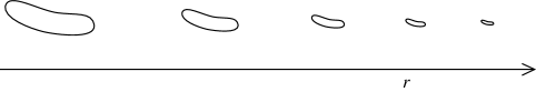
FIG. 8.: An optical illusion: all the strings are the same size. Strings of constant size in an inertial frame, at different radial positions $r$, have different coordinate sizes.

This power-law effect is true both for the elastic scattering studied in ref. [2] and for the inelastic scattering considered here. However, in the elastic case the scaling in the string limit is qualitatively the same as in the parton model. The reason is that in both the parton and string limits, elastic scattering at large momentum transfer requires the entire hadron to shrink to small size, and so is determined by the overall dimensional scaling of the hadron wave function. In both cases the magnitude of the wavefunction in this region is determined simply by the conformal dimension of the gauge-invariant operators which can create the state. For hadrons that mix with chiral states of the superconformal algebra, this dimension is the same at large and small ’t Hooft parameter; more generally the powers involved are of order 1 but are never zero.

However, in inelastic scattering it is not necessary for the entire hadron to shrink to small size. The photon may strike only a fraction of the hadron, leading to different dimensional scaling. In the parton limit, the photon may strike as little as a single parton. The probability that one parton will be small while the rest of the hadron is large is clearly greater than the probability that the entire hadron is small, or even that two partons shrink together to a small size; thus one-parton scattering dominates. Since the operators which create and destroy a single parton can have twist 2 in this limit, they lead to Bjorken scaling. By contrast, in the string limit, as evident from Fig. 3, the probability that a small fraction of the string will tunnel to large $r$ while the rest remains at small $r$ is highly suppressed. This implies the four-dimensional hadron does not contain pointlike partons at large ’t Hooft parameter. This corresponds to the fact that operators which couple to one or more partons in a gauge-non-invariant combination have large twist. The string is able to scatter inelastically only in the same way as it scatters elastically, by tunneling to large $r$ where its projection onto $x^{\mu}$ is small, and then scattering as a unit. As in the elastic case, the magnitude of the wavefunction in this region is determined simply by the conformal dimension of the state. The entire hadron must shrink to a size of order $q^{-1}$; our calculation shows that the probability of this is $q^{-2(\tau_{p}-1)}$. Since the gauge-invariant operators which can create a hadron in ${\cal N}=1^{*}$ and many similar theories have $\tau_{p}\geq 2$, we never recover Bjorken scaling in the string limit. (Note that formally a hadron with $\tau_{p}=1$ behaves as a single pointlike parton, as in other contexts.)

In the leading large-$N$ limit we are studying the internal dynamics of a single string, with string production turned off. From the OPE analysis we concluded that at finite $N$ a subleading piece would ultimately dominate at large $q^{2}$. The corresponding supergravity process is depicted in Fig. 4. The incoming hadron splits into two, one of which (B) has the minimum twist $\tau_{\rm c}$ of any charged hadron. (In ${\cal N}=1^{*}$, for example, the lowest-twist charged hadron is a $\Delta=2$ state of the dilaton.) Hadron B then tunnels to large $r$ and interacts with the current. The interaction of B with the the external current should be essentially the same as above with $\tau_{\rm c}$ in place of $\Delta$. The splitting of the initial hadron into A and B occurs in the IR region and so depends on details of the model. This can presumably be encoded into a distribution function for B to carry a fraction $x$ of the incoming energy, which we simply need to convolve with the above result at $\tau=\tau_{\rm c}$. We have not attempted to calculate the distribution function, but we believe it can be done within the supergravity approximation.

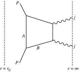
FIG. 9.: Subleading contribution in $N$. The incoming hadrons splits into hadrons A and B, with B having minimum twist $\tau_{\rm c}$.

The $q^{2}$ dependence thus reproduces what we deduced from the OPE. We now consider the remaining details of the string result. First, we see that the function $F_{2}$ is the same for both the dilaton and dilatino. This is reasonable, since (as can be seen by expanding the propagator of the scattered particle in powers of the external photon) the function $F_{2}$ generally measures spin-independent information. By contrast, $F_{1}$ is proportional to the Casimir of the scattered object under the Lorentz group, so it vanishes for the scalar hadron, as it also would for a scalar parton. The distinction between spinor parton and spinor hadron scattering (aside from the $q^{2}$ dependence) shows up in the modification of the Callan-Gross relation. A scattered parton in the parton model has momentum $xP$, while in our case the scattered hadron has momentum $P$. This missing factor of $x$ is the same one missing from the Callan-Gross relation in our computation (83).

We do not have a physical interpretation of the full $x$-dependence of our result, but we can understand the behavior near $x=1$. For $x\sim 1$ the mass-squared of the intermediate state is

$$s=q^{2}(1-x)\ .$$ (84)

If we take $q^{2}\to\infty$ with $s$ held fixed (so that $1-x\to 0$), then the matrix element $\langle P_{X},X|\tilde{J}^{\mu}(q)|P,{\cal Q}\rangle$ is essentially a hard form factor, and is governed by the same kind of scaling as the elastic amplitudes [2, 13]. In this limit, the Bessel function in the wavefunction for $X$ becomes a power law, just as for the initial hadron. This reflects the fact that in this kinematic regime both the initial hadron and the hadron $X$ have to shrink down to size $q^{-1}$ in order to scatter from the photon. It follows that the matrix element is determined by the conformal weight, falling as $q^{2-2\tau_{p}}$, and so the structure function is

$$F_{2}=q^{6-4\tau_{p}}G_{2}(q^{2}[1-x])$$ (85)

for some function $G_{2}$. But we also know from the OPE that $F_{2}$ scales as $q^{2-2\tau_{p}}$, so it must be that $G_{2}\propto(q^{2}[1-x])^{\tau_{p}-2}$ which is indeed the behavior found as $x\to 1$. This same argument applies at small ’t Hooft parameter (where $\tau_{p}$ is the number $n$ of partons in the initial hadron), but at the final step we require instead that $F_{2}$ be independent of $q^{2}$, giving $G_{2}\propto(q^{2}[1-x])^{2n-3}$ and $F_{2}\propto(1-x)^{2n-3}$, up to the usual perturbative scaling violations [15].

V The Regge Region

Our analysis is incomplete in an important respect. We have noted that the energy-momentum tensor has no anomalous dimension, and therefore the moments

$$M^{(1)}_{2}=\int_{0}^{1}dx\,xF_{1}(x,q^{2})\ ,\quad M^{(2)}_{2}=\frac{1}{2}\int_{0}^{1}dx\,F_{2}(x,q^{2})$$ (86)

have nonzero limits as $q^{2}\to\infty$, determined by the $J^{\mu}J^{\nu}T^{\rho\sigma}$ operator product coefficient. This is not the case for our result (69), which gives moments that falls as $q^{2-2\Delta}$. Such a falloff is correct for the higher moments, with additional powers of $x$, so it must be that we have missed a component of $F_{1,2}$ that is narrowly peaked around $x=0$.

The existence of such a component is also suggested by a more physical argument [8]. At small coupling, interactions cause partons to split and so the structure functions evolve toward smaller $x$. As the interactions become strong, this evolution becomes more rapid. With very strong interactions, the parton language becomes inapplicable, but one might still expect a rapid evolution toward small $x$, leaving most of the weight of the $F_{i}$ at near $x=0$. The moments (86) must be conserved by this flow.

The calculation in the previous section is valid as long as the supergravity approximation holds. However, for sufficiently small $x$, this will no longer be the case. Eq. (56) shows that the scattering energy from the point of view of the local observer in the bulk becomes of order the string mass scale when $x\sim(gN)^{-1/2}$. Beyond this point, one must take seriously the fact that the bulk theory is a string theory. Since DIS is extracted from a forward scattering amplitude, it is the Regge physics of the string which is important here.

In fact this point is used in standard QCD to argue that the small-$x$ behavior of the gluon structure function is dominated by Pomeron exchange [22, 16]. This is mainly kinematics: the center-of-mass energy-squared of the photon-hadron system in the DIS process is $s\approx q^{2}/x$ as $x\to 0$, so the small $x$ region is the large $s$ region. The Pomeron — a trajectory of conjectured glueball states of increasingly higher spin, analogous to the graviton trajectory of string theory — gives a contribution to parton distribution functions of the form $f(x,q^{2})\sim x^{-\alpha_{0}}$, where $\alpha_{0}$ is the intercept of the Pomeron trajectory with the spin axis in the $M^{2}$ vs. $J$ Regge plot. The variation with $q^{2}$ is not specified by general arguments, but it has been argued [22] that in QCD it should be slow. Since Pomeron exchange also predicts that the total proton-proton cross-section should grow as $s^{\alpha_{0}}$, the intercept can be extracted from data (giving something of order $1.1$) or predicted from QCD (giving something of order $1.4$.) The interpretation of these discrepant values is controversial. For our purposes it suffices that $\alpha_{0}$ in QCD is closer to 1 than to 2. That the gluon structure function grows faster than $x^{-1}$ but quite a bit slower than $x^{-2}$ is in fact observed at HERA.

In ${\cal N}=1^{*}$, one could in principle compute the Pomeron intercept at small $gN$ using the perturbative techniques outlined in [16]; we have not done this. The large $gN$ region is much easier, however. The Pomeron trajectory is the graviton trajectory; more precisely, it is the trajectory whose lowest state is the lowest-lying spin-two glueball, given as the lowest mode of the graviton inside the cutoff five-dimensional $AdS$ space. An exactly massless spin-two mode would give an intercept of exactly two. The IR cutoff on the $AdS_{5}\times W$ space produces a mass gap of order $R^{-2}$ in the bulk, and so lowers the intercept of the trajectory by order $\alpha^{\prime}/R^{2}\sim(gN)^{-1/2}$. The intercept is therefore $2-{\rm order}(gN)^{-1/2}$, and so we therefore expect that the DIS amplitudes will have the behavior

$$xF_{1}\sim F_{2}\propto x^{-1+O(gN)^{-1/2}}$$ (87)

at small $x$. While we will see that this is true, the full story is somewhat more subtle.

An important caveat is that we will consider only the leading effect in the large-$N$ limit, corresponding to string tree level. In other words, we are focusing on the internal structure of a single string. Because of the growth of the amplitude with energy, the production of multiple strings (and ultimately black hole formation [17]), corresponding to multi-Pomeron exchange, shadowing, etc., dominates at asymptotically large $s$ (small $x$) for any finite $N$. We will not address these phenomena here. For other approaches to fixed momentum transfer scattering in AdS/CFT, see Ref. [18].

A Calculation at small $x$

In the supergravity calculation we explicitly summed over intermediate states $X$, which were radial KK excitations, but in the string case it is simpler to sum implicitly by taking the imaginary part of the forward four-point amplitude. The momentum invariants in the inertial frame are of order the string scale, so we might expect the scattering process to be localized on this scale. Since this is small compared to the AdS radius, we can take the flat spacetime string amplitude and fold it into the AdS wavefunctions. Actually, we will see that at exponentially small $x$ this locality breaks down, but for now we will assume it.

The string interaction can be written [19]

$${\cal L}_{\rm eff,string}=KG$$ (88)

with $K$ a kinematic factor and

$$G=-\frac{\alpha^{\prime 3}\tilde{s}^{2}}{64}\prod_{\xi=s,t,u}\frac{\Gamma(-\alpha^{\prime}\tilde{\xi}/4)}{\Gamma(1+\alpha^{\prime}\tilde{\xi}/4)}\ ;$$ (89)

the prefactor is included for later convenience. The tildes are included on the Mandelstam variables because this flat spacetime amplitude goes over to the inertial frame quantity in curved spacetime. Expanding around $\tilde{t}=0$, one finds, for $\tilde{s}$ near the positive real axis,

$$G=-\left[{1\over\tilde{t}}+\pi\cot\left({\pi\alpha^{\prime}\tilde{s}\over 4}\right)\right]\left[{\alpha^{\prime}\tilde{s}\over 4e}\right]^{\alpha^{\prime}\tilde{t}/2}\left[1+{\rm order}(\alpha^{\prime}\tilde{t})\right]$$ (90)

(To obtain this expression we have used Stirling’s approximation, but when $\alpha^{\prime}|\tilde{t}|\ll 1$ the form is valid even for $\alpha^{\prime}\tilde{s}\sim 1$.) The imaginary part from excited strings is

$${\rm Im}_{\rm exc}\,G|_{\tilde{t}\to 0}=\frac{\pi\alpha^{\prime}}{4}\sum_{m=1}^{\infty}\delta(m-\alpha^{\prime}\tilde{s}/4)\ ({m})^{\alpha^{\prime}\tilde{t}/2}\ \ .$$ (91)

The last factor — the small-angle Regge behavior of the string amplitude — becomes important at ultra-small $x$. This is because, as we will see later, the ten-dimensional $\tilde{t}$ is not quite zero, even though $t=0$. Instead, it will turn out that $\alpha^{\prime}\tilde{t}\sim(gN)^{-1/2}.$ This implies that when $\alpha^{\prime}\tilde{t}\log(\alpha^{\prime}\tilde{s})\gtrsim 1$, that is, for $\tilde{s}\sim 1/x$ exponentially large, of order $e^{\sqrt{gN}}$, we must include this term. For $e^{-\sqrt{gN}}\ll x\ll{1\over\sqrt{gN}}$, however, we can ignore it.

To obtain the imaginary part of the forward amplitude we must evaluate $K|_{\tilde{t}=0}$. One can do this directly from the definition [19] or by noting from the expansion (90) that it is the same as the coefficient of the $t$-channel graviton pole. One finds

$$K|_{\tilde{t}=0}=\frac{1}{8}\int d^{10}x\,\Bigl{\{}4v^{a}v_{a}\,\partial_{m}\Phi F^{mn}F_{pn}\partial^{p}\Phi-(\partial^{M}\Phi\partial_{M}\Phi\,v^{a}v_{a}+2v^{a}\partial_{a}\Phi\,v^{b}\partial_{b}\Phi)F_{mn}F^{mn}\Bigr{\}}\ ,$$ (92)

with the same index conventions as in Section IV. The dilaton is canonically normalized and the normalization of the vector potential is defined by the Kaluza-Klein ansatz (40). We have written this as an effective action in position space to facilitate the lift to curved spacetime. At small $x$, the first term in the effective action (92) dominates, because the index structure gives two extra factors of $P\cdot q$; thus we will focus on this term. Notice that the explicit dependence on ${\cal Q}$, through $v^{a}\partial_{a}\Phi_{\rm i}=i{\cal Q}\Phi_{\rm i}$, is subleading — as in QCD, the wee parton cloud is universal and does not depend on the quantum numbers of the hadron.

Evaluating this effective Lagrangian in the AdS matrix element gives the contribution of excited strings to the imaginary part of the forward current-current amplitude. For $x$ not exponentially small, we drop the $\tilde{s}^{\alpha^{\prime}\tilde{t}}$ factor and obtain

$$n_{\mu}n_{\nu}{\rm Im}_{\rm exc}{\sf T}^{\mu\nu} = (K\,{\rm Im}\,G)|_{\tilde{t}=0}$$ (93)

$$= \frac{\pi\alpha^{\prime}}{2}\sum_{m=1}^{\infty}\int d^{6}x_{\perp}\sqrt{-g}\,v^{a}v_{a}\,\partial_{m}\Phi^{*}_{\rm i}F^{mn}(-q)\delta(m-\alpha^{\prime}\tilde{s}/4)F_{pn}(q)\partial^{p}\Phi_{\rm i}\ .$$ (94)

All contractions are now with the full ten-dimensional metric. The invariant $\tilde{s}$ in principle involves a differential operator acting on the fields to its right,

$$\alpha^{\prime}\tilde{s}=\frac{\alpha^{\prime}sR^{2}}{r^{2}}+\frac{\alpha^{\prime}}{R^{2}}(r^{2}\partial_{r}^{2}+5r\partial_{r}+\hat{\nabla}_{W}^{2})\ .$$ (95)

Everything is smooth in the radial direction, so $r\partial_{r}=O(1)$, and the dimensionless Laplacian on $W$ is similarly assumed to be $O(1)$. Consequently, $\alpha^{\prime}\tilde{s}={\alpha^{\prime}s}(R^{2}/r^{2})$ plus corrections of order $\alpha^{\prime}/R^{2}\sim(gN)^{-1/2}$, which for excited strings can be neglected compared to the integer $m$ in the delta function. This is consistent with our argument that the effective interaction is local on the AdS scale. (The case $m=0$ is not covered by this argument, but we have already calculated it explicitly, without this assumption, in Section IV.) The delta function then becomes $\delta(m-\alpha^{\prime}sR^{2}/4r^{2})$, and so just fixes the radial integration.

We can now evaluate the amplitude (94). The components of the field strength are

$$F_{\mu\nu}(q)=i(q_{\mu}n_{\nu}-n_{\mu}q_{\nu})\frac{qR^{2}}{r}K_{1}(qR^{2}/r)e^{iq\cdot y}\ ,$$ (96)

$$F_{\mu r}(q)=(n_{\mu}q^{2}-q_{\mu}q\cdot n)\frac{R^{4}}{r^{3}}K_{0}(qR^{2}/r)e^{iq\cdot y}\ .$$ (97)

which implies

$$F_{\mu p}F_{\nu}{}^{p} = \biggl{(}n_{\mu}-q_{\mu}\frac{q\cdot n}{q^{2}}\biggr{)}\biggl{(}n_{\nu}-q_{\nu}\frac{q\cdot n}{q^{2}}\biggr{)}\frac{w^{4}}{R^{2}}[K_{0}^{2}(w)+K_{1}^{2}(w)]$$ (99)

$$\qquad\qquad+{q^{\mu}q^{\nu}}\biggl{(}n^{2}-\frac{q\cdot n\,q\cdot n}{q^{2}}\biggr{)}\frac{w^{4}}{q^{2}R^{2}}K_{1}^{2}(w)$$

where $w=qR^{2}/r$. (The contributions of $F_{rp}F_{\nu}{}^{p}$ and $F_{rp}F_{r}{}^{p}$ are negligible). Then

$$n_{\mu}n_{\nu}{\rm Im}_{\rm exc}{\sf T}^{\mu\nu} = \frac{\pi\rho|c_{\rm i}|^{2}}{8}\Biggl{(}\frac{\Lambda^{2}}{q^{2}}\Biggr{)}^{\Delta-1}\,\sum_{m=1}^{\infty}w_{m}^{2\Delta+2}\Biggl{\{}\frac{1}{x}K^{2}_{1}(w_{m})\biggl{(}n^{2}-\frac{q\cdot n\,q\cdot n}{q^{2}}\biggr{)}$$ (101)

$${\qquad\qquad\qquad}+\frac{4x}{q^{2}}\Bigl{[}K^{2}_{0}(w_{m})+K^{2}_{1}(w_{m})\Bigr{]}\biggl{(}P\cdot n-\frac{P\cdot q\,n\cdot q}{q^{2}}\biggr{)}^{2}\Biggr{\}}\ ,$$

where $w_{m}=qR^{2}/r_{m}$ and $r_{m}={R(\alpha^{\prime}s)^{1/2}}/{2m^{1/2}}$. The dimensionless constant $\rho$ is from the angular integral

$$\int d^{5}\Omega\sqrt{\hat{g}_{W}}\,v^{a}v_{a}|Y|^{2}=\rho R^{2}$$ (102)

(note that $v^{a}$ and $\partial_{a}\psi$ are $R$-independent). The structure functions are then

$$F_{1} = \frac{\pi^{2}\rho|c_{\rm i}|^{2}}{4x}\Biggl{(}\frac{\Lambda^{2}}{q^{2}}\Biggr{)}^{\Delta-1}\sum_{m=1}^{\infty}w_{m}^{2\Delta+2}K^{2}_{1}(w_{m})\ ,$$ (103)

$$F_{2} = \frac{\pi^{2}\rho|c_{\rm i}|^{2}}{2}\Biggl{(}\frac{\Lambda^{2}}{q^{2}}\Biggr{)}^{\Delta-1}\sum_{m=1}^{\infty}w_{m}^{2\Delta+2}\Bigl{[}K^{2}_{0}(w_{m})+K^{2}_{1}(w_{m})\Bigr{]}\ .$$ (104)

The argument of the Bessel functions is $w_{m}\sim x^{1/2}m^{1/2}/(gN)^{1/4}$, and so when $x\ll(gN)^{-1/2}$ the sums can be approximated by integrals. Using

$$I_{j,n}=\int_{0}^{\infty}dw\,w^{n}K_{j}^{2}(w)=2^{n-2}\frac{\Gamma(\nu+j)\Gamma(\nu-j)\Gamma(\nu)^{2}}{\Gamma(2\nu)}\ ,\quad\nu=\frac{1}{2}(n+1)\ .$$ (105)

so that $I_{1,n}={n+1\over n-1}I_{0,n}$, one finds

$$F_{1} = \frac{1}{x^{2}}\,\Biggl{(}\frac{\Lambda^{2}}{q^{2}}\Biggr{)}^{\Delta-1}\frac{\pi^{2}\rho|c_{\rm i}|^{2}}{4(4\pi gN)^{1/2}}I_{1,2\Delta+3}\ ,$$ (106)

$$F_{2} = 2x{2\Delta+3\over\Delta+2}F_{1}\ .$$ (107)

B Exponentially small $x$

As expected, the inclusion of excited strings leads to a new term in the structure functions, which dominates at small $x$. This has an interesting effect on the moments $M_{n}^{(1,2)}$. For $n>2$, the new contribution converges and gives the same $q^{2-2\Delta}$ dependence as found in the supergravity calculation; this corresponds again to the double-trace operators found in section III. However, the momentum sum $n=2$ now diverges as $x\to 0$. Thus we need to understand how the calculation that we have done breaks down in this limit.

We emphasize again that we consider only the leading effect in the large-$N$ limit, corresponding to the internal structure of a single string. Since the amplitudes grow with energy and we will now study values of $x$ that are exponentially small in $(gN)^{1/2}$, the following calculation is the dominant process only for $N$ that is exponentially large. Thus we are looking at an extreme region of parameter space, but one that is conceptually interesting.

Note that the $x$-dependence of the structure functions (107) agrees to leading order with the field theory expectation (87). However, the $O(gN)^{-1/2}$ correction to the exponent is crucial to the convergence of the momentum sum rule. It appears that we need to go to the next order in the ’t Hooft parameter, which is a daunting task. However, we will argue that the crucial correction enters in a simple way. We will first support this by heuristic arguments, and after carrying out the improved calculation we will give a more formal justification using the string world-sheet OPE.

We claim that we simply need to keep the full Regge form of the string amplitude by restoring the Regge factor in (90). The Regge factor is nontrivial because, although the four-dimensional $t$ vanishes by definition, the ten-dimensional $\tilde{t}$ includes in addition derivatives in the transverse directions, as with $\tilde{s}$ in (95). This $\tilde{t}$ is small on the string scale, of order $(gN)^{-1/2}$, but its effect becomes large when $\tilde{s}$ is exponentially large in $(gN)^{1/2}$, or equivalently when $x$ is exponentially small. This modification clearly has the right form to produce the Regge correction to the $x$-dependence of the structure function, and we will argue later that it is the only important correction.

Notice that the modification is nonlocal, because it involves a power of the differential operator $\tilde{t}$. This is the logarithmic spreading of strings in the Regge region [5]. Thus the assumption that the interaction is approximately local breaks down, though in a way that is fairly simple to incorporate by replacing $\tilde{t}$ with a curved spacetime Laplacian. The need for such nonlocality can be understood in various ways. For one, local interactions will always contain a factor of $q^{-2\Delta}$ and so cannot give $q$-independent moments. This is because the falloff of the vector potential requires that the interaction occur at $r\gtrsim R^{2}q$, and so we only pick up the $r^{-\Delta}$ tail of each wavefunction. For another, the real part of the amplitude is nonlocal, from graviton exchange. That is, the vector background induces a metric perturbation at second order, which can propagate to smaller $r$ without exponential suppression. By analyticity we expect a similar effect in the imaginary part.

Our prescription is then to modify (94) by inserting $\tilde{s}^{\alpha^{\prime}\tilde{t}/2}\sim x^{-\alpha^{\prime}\tilde{t}/2}$, averaging over the delta functions (since we are at exponentially large $m$) and writing $\tilde{t}$ as a differential operator acting in the $t$-channel:

$$n_{\mu}n_{\nu}{\rm Im}_{\rm exc}{\sf T}^{\mu\nu}=\frac{\pi\alpha^{\prime}}{2}\int d^{6}x_{\perp}\sqrt{-g}\,v^{a}v_{a}\,F^{mn}(-q)F^{p}{}_{n}(q)\,x^{-\alpha^{\prime}\nabla^{2}/2}(\partial_{m}\Phi^{*}_{\rm i}\partial_{p}\Phi_{\rm i})\ .$$ (108)

In the correction term we have replaced $\alpha^{\prime}\tilde{s}$ with $1/x$ because the exponentially large parts of these are the same:

$$\alpha^{\prime}\tilde{s}\sim\alpha^{\prime}sR^{2}/r_{\rm int}^{2}\sim\alpha^{\prime}s/R^{2}q^{2}\sim 1/(gN)^{1/2}x\ ;$$ (109)

they differ by a power of the ’t Hooft parameter, which is large but not exponentially so.

We need to identify the Laplacian that appears. The dominant components of $\partial_{m}\Phi^{*}_{\rm i}\partial_{p}\Phi_{\rm i}$ at small $x$ are $\partial_{\mu}\Phi^{*}_{\rm i}\partial_{\nu}\Phi^{\vphantom{*}}_{\rm i}=P_{\mu}P_{\nu}\Phi^{*}_{\rm i}\Phi^{\vphantom{*}}_{\rm i},$ because these contract with $q^{\mu}q^{\nu}$ to give a factor $s^{2}$. Since $P^{2}$ is negligible, the dilaton and graviton-trace do not couple and so we need the Laplacian for four-dimensional traceless symmetric tensors. Working out the connection, one finds

$$\nabla^{2}(P_{\mu}P_{\nu}\Phi^{*}_{\rm i}\Phi^{\vphantom{*}}_{\rm i})=P_{\mu}P_{\nu}e^{2A}\nabla_{0}^{2}(e^{-2A}\Phi^{*}_{\rm i}\Phi^{\vphantom{*}}_{\rm i})\equiv P_{\mu}P_{\nu}D^{2}(\Phi^{*}_{\rm i}\Phi^{\vphantom{*}}_{\rm i})\ ,$$ (110)

where $e^{2A}$ is a general warp factor as in Eq. (51), $\nabla_{0}^{2}$ is the scalar Laplacian, and we have defined $D^{2}=e^{2A}\nabla_{0}^{2}e^{-2A}$.

The exponential of $\nabla^{2}$ is nonlocal, essentially a diffusion operator, with $\ln x$ as diffusion time. Consequently the details of the geometry in the region where conformal symmetry is broken can enter when the diffusive “time” becomes large. Still, we can continue to use the $AdS_{5}\times W$ form (99) for the field strength, since its exponential falloff for $r<R^{2}q$ means it is unaffected by the conformal symmetry breaking. We then have

$$F_{1}=\frac{\pi^{2}\alpha^{\prime}R^{4}q^{2}}{4x^{2}}J_{1}\ ,\quad F_{2}=\frac{\pi^{2}\alpha^{\prime}R^{4}q^{2}}{2x}(J_{0}+J_{1})\ ,$$ (111)

where

$$J_{i}=\int dwd^{5}\Omega\sqrt{\hat{g}_{W}}\,v^{a}v_{a}\,w^{3}K_{i}^{2}(w)\,x^{-\alpha^{\prime}D^{2}/2}(\Phi^{*}_{\rm i}\Phi^{\vphantom{*}}_{\rm i})\ .$$ (112)

Omitting the correction term, one readily recovers the earlier result (107).

Now let us consider the asymptotic behavior as $x\to 0$. The $x$ dependence will be determined by the smallest eigenvalue $\lambda$ of $-\nabla^{2}$, of order $R^{-2}$, i.e., $\alpha^{\prime}\lambda\sim(gN)^{-1/2}$. Thus we have

$$F_{1}\propto x^{-2+\alpha^{\prime}\lambda/2}\ ,\quad F_{2}\propto x^{-1+\alpha^{\prime}\lambda/2}\ .$$ (113)

This is of the expected form (87), and we identify the Pomeron intercept as $2-\alpha^{\prime}\lambda/2$. To get the $q$-dependence in this limit, we note that the lowest normalizable eigenfunction of $\nabla_{0}^{2}$ falls as $r^{-4}$ as $r\to\infty$, and so the lowest normalizable eigenfunction of $D^{2}$ falls as $r^{-2}$. Then, up to $x$- and $q$-independent factors,

$$J_{i}\propto x^{\alpha^{\prime}\lambda/2}\int dwd^{5}\Omega\sqrt{\hat{g}_{W}}\,v^{a}v_{a}w^{3}K_{i}^{2}(w)\,r^{-2}\ .$$ (114)

The integral is dominated by $w\sim 1$, where $r^{-2}\sim R^{-4}q^{-2}$. Thus $F_{1,2}$ given by Eq. (111) are independent of $q^{2}$ in this limit, and so we will get indeed get a $q^{2}$-independent moment.

Before $x$ reaches the point where the conformal symmetry breaking region is felt by the diffusion operator, but at $x$ small enough that the $x^{-\alpha^{\prime}\nabla^{2}/2}$ is not negligible, there is a rexgime where the diffusion occurs entirely in the AdS region. In this case we can obtain a simple and interesting expression for the structure functions. In the AdS region,

$$D^{2}=R^{-2}(\partial_{u}^{2}-4)\ ,\quad u=\ln(r/r_{0})\ ,$$ (115)

and so

$$x^{-\alpha^{\prime}D^{2}/2}(\Phi^{*}_{\rm i}\Phi^{\vphantom{*}}_{\rm i})=x^{\alpha^{\prime}\zeta/2}\,\Phi^{*}_{\rm i}\Phi^{\vphantom{*}}_{\rm i}\ ,\quad\zeta=\frac{4}{R^{2}}(1-\Delta^{2})\leq 0\ .$$ (116)

Compared to the calculation in Section V.A, the only effect is a rescaling, so (107) is slightly modified:

$$F_{1} = x^{-(2+\alpha^{\prime}|\zeta|)/2}\Biggl{(}\frac{\Lambda^{2}}{q^{2}}\Biggr{)}^{\Delta-1}\frac{\pi^{2}\rho|c_{\rm i}|^{2}}{4(4\pi gN)^{1/2}}I_{1,2\Delta+3}\ ,\ F_{2}=2x{2\Delta+3\over\Delta+2}F_{1}\ .$$ (117)

Note that since $\zeta<0$, its effect on the structure functions in the range where the form (117) is valid makes them grow more rapidly at small $x$. The reason is simple. The wavefunction $\Phi_{\rm i}$ is largest at small $r$, where the gauge field is negligibly small. The diffusion operator, which represents the logarithmic growth of strings, allows this larger part of the wavefunction to interact with the gauge field, and so increases the amplitude. This effect shuts off, giving the other behavior (113), when the diffusion reaches from the IR cutoff $r_{0}$ all the way to the interaction radius $R^{2}q$ — this is at very small $x$, corresponding to large diffusion time. The $\zeta<0$ growth is needed to connect the small-$x$ form, which falls with $q$, to the $q$-independent behavior at exponentially small $x$.

Finally let us evaluate the moments $M^{(i)}_{2}$. Using the structure functions (111) yields

$$M^{(1)}_{1} = \frac{\pi^{2}R^{4}q^{2}}{2}\int dwd^{5}\Omega\sqrt{\hat{g}_{W}}\,v^{a}v_{a}\,w^{3}K_{0}^{2}(w)\frac{1}{-D^{2}}\Phi^{*}_{\rm i}\Phi^{\vphantom{*}}_{\rm i}$$ (118)

$$M^{(2)}_{2} = \frac{\pi^{2}R^{4}q^{2}}{2}\int dwd^{5}\Omega\sqrt{\hat{g}_{W}}\,v^{a}v_{a}\,w^{3}\Bigl{(}K_{0}^{2}(w)+K_{1}^{2}(w)\Bigr{)}\frac{1}{-D^{2}}\Phi^{*}_{\rm i}\Phi^{\vphantom{*}}_{\rm i}\ .$$ (119)

This has a simple graphical interpretation. The $1/D^{2}$ is a graviton propagator, so this is the graph shown in Fig. 5. The right vertex is the AdS/CFT representation of the $J^{\mu}J^{\nu}T^{\rho\sigma}$ OPE coefficient, while the left vertex is determined by the total energy-momentum of the hadron. Thus we have reproduced the expected form.

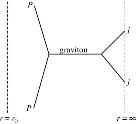
FIG. 10.: Feynman graph giving the moment $M_{2}$.

To evaluate the moment explicitly, we must first solve

$$-D^{2}h=\Phi^{*}_{\rm i}\Phi^{\vphantom{*}}_{\rm i}$$ (120)

for $h(r,\Omega)$. Integrating this equation over the interior of a sphere of radius $r_{\rm c}$ gives

$$-\int_{r<r_{\rm c}}drd^{5}\Omega\sqrt{-g}\,\nabla_{0}^{2}(e^{-2A}h)=\int_{r<r_{\rm c}}drd^{5}\Omega\sqrt{g_{\perp}}e^{2A}\Phi^{*}_{\rm i}\Phi^{\vphantom{*}}_{\rm i}\ .$$ (121)

Taking $r_{\rm c}\gg r_{0}$, the right-hand side becomes the normalization integral (50) and is equal to unity. On the left-hand side, at $r\gg r_{0}$ the function $h$ goes over to the normalizable AdS form for the graviton, proportional to $1/r^{2}$, with the normalization fixed by Eq. (121) to be

$$h=\frac{1}{-D^{2}}\Phi^{*}_{\rm i}\Phi^{\vphantom{*}}_{\rm i}\to\biggl{(}4r^{2}R^{2}\int_{W}d^{5}\Omega\sqrt{\hat{g}_{W}}\biggr{)}^{-1}\ .$$ (122)

As $q^{2}\to\infty$, the Bessel functions cut off the integral (112) in the AdS region and so we can use the asymptotic form (121). One then finds

$$M_{2}^{(1)}\to\frac{\pi^{2}}{5}\frac{\displaystyle\int_{W}d^{5}\Omega\sqrt{\hat{g}_{W}}\,\hat{g}_{Wab}\,v^{a}v^{b}}{\displaystyle\int_{W}d^{5}\Omega\sqrt{\hat{g}_{W}}}\ ,\quad\frac{M_{2}^{(2)}}{M_{2}^{(1)}}\to\frac{5}{3}\ .$$ (123)

Note that the moments are completely independent of the initial hadron. They depend only on the current, through the Killing vector $v^{a}$, which is consistent with their relation to an OPE coefficient. We conclude that our understanding of the distribution functions is complete, in the large $N$ limit.

Now let us understand from a somewhat more formal point of view the nature of the string calculation that we are doing. Because the size of the excited strings is of order the curvature radius of the spacetime, we must do a true string calculation, with vertex operators for the four external states, on a sphere. Three of these operators, say two gauge vertex operators and one dilaton, can be fixed, and the world-sheet coordinate $z$ of the remaining dilaton is integrated. Because the spacetime curvature is small in string units, the world-sheet coupling $(gN)^{-1/2}$ is also small. However, there is another small parameter in the problem, namely $x$, and we wish to keep corrections that are large when $x^{(gN)^{-1/2}}$ differs significantly from unity. In other words, we want to keep all orders in $(gN)^{-1/2}\ln x$ while treating $(gN)^{-1/2}$ itself as small.

This is reminiscent of the renormalization group, and indeed it is precisely that on the world-sheet. A standard saddle point estimate shows that in the Regge regime the world-sheet path integral is dominated small separation of the two dilaton vertex operators, $\delta z\sim\tilde{t}/\tilde{s}\sim x$. We can then carry out the calculation in steps, the first of which is to use the OPE to replace the product of dilaton vertex operators with a single $t$-channel vertex operator (the operators that contribute are those of the graviton Regge trajectory). To avoid large logs, this operator itself must be renormalized at a scale comparable to the separation $\delta z$. It is then necessary to run this operator to a reference scale of order the radius of the sphere, and the final three-point amplitude has no large logs. The large logs of $x$ come only from the running of the vertex operator. This is precisely our correction factor $x^{-\alpha^{\prime}\nabla^{2}/2}$ — the exponent is the world-sheet anomalous dimension of the $t$-channel vertex operator. This justifies our prescription (108).

VI Outlook

Let us summarize the results of the string calculations, in particular with regard to the different ranges of $x$.

  A.

At $x\gg(gN)^{-1/2}$ we have the supergravity results (69), (83).

  B.

At $x\ll(gN)^{-1/2}$ but with $|\ln x|\ll(gN)^{1/2}$ we have the form (107), where the excited strings form a continuum.

  C.

When $|\ln x|(gN)^{-1/2}$ becomes of order one we must take into account the effect of string growth, leading to the form (117).

  D.

Finally, when $|\ln x|(gN)^{-1/2}>\ln(\Lambda/q)$ we go over to the final asymptotic form (113).

The behavior B is actually a special case of C, in that the form (117) reduces to (107) when $|\ln x|(gN)^{-1/2}$ is small. The transition between forms A and B is described by a discrete sum over excited strings, Eq. (104). The transition between C and D would similarly be described by a discrete sum over eigenvalues of $D^{2}$.

In region A, we have found a transition at $gN\sim 1$ — more precisely, a crossover — from partonic to hadronic behavior. This crossover is interesting from a number of points of view. For one thing, it is related to a string theory crossover, in which a set of $N$ D-branes with small string coupling should be replaced, when $gN\gg 1$, by a black brane with a large gravitational field and a horizon. There are important long-standing questions about this mysterious transition. Where did the branes, and the open strings on their world-volume, go? Which aspects of the physics are the same on both sides of $gN\sim 1$, and which are fundamentally different? Along the same lines is the question of precisely how, for any computation in this background, a result calculated on worldsheets with boundaries and holes at small $gN$ can be calculated with worldsheets with no holes at large $gN$; how do the holes close, or become subleading?

Although we have not concretely answered these questions, we have related them to a system which is easier to understand — the operator spectrum of the world-volume field theory. We have done so using nonperturbative methods in field theory, making it possible to qualitatively follow the transition from small to large $gN$. The shifting of operator dimensions relative to one another is easy to understand and describe, even at the point of transition where the physics is complicated in both perturbative field theory and in perturbative string theory.

Using this knowledge one can roughly understand which classes of Feynman graphs, or more precisely, which regions of kinematics within those Feynman graphs, are suppressed as $gN\to 1$. In this regime, the probability for parton emission is so great, for any colored line whose color is not immediately cloaked, that any hole in the worldsheet — any place where a color index is carried by something physically separated from the corresponding anticolor — becomes densely filled with multiple partons. Note this has nothing to do with confinement; there are no flux tubes here. It is simply that the probability that a light color charge will radiate other light colored particles is so great that no such particle will ever be isolated. Thus it seems the holes in the worldsheet — the holes between colored particles in Feynman graphs — fill in not because they shrink (with the gluons, thin ribbons in ’t Hooft’s double-line formalism, somehow becoming thick) but because they are broken up into tiny fragments, as though covered over by cheesecloth, as a myriad of additional thin ribbons are emitted. To localize and scatter off a parton with substantial $x$ inside a hadron requires separating it from its neighbors; this will not happen in the large $gN$ regime. Again, we stress this has nothing to do with confinement; this is also clear from the fact that ${\cal N}=4$ Yang-Mills is described by closed strings at large $gN$.

From a particle physicist’s point of view, the interest of these results lies in two places. On the one hand, they gives some conceptual insights into QCD. We have shown that, at large $gN$, DIS in the moderate $x$ region is quite different from QCD. This is true despite the fact that various scaling laws, such as the “parton-counting” rules [23, 24], are still valid in this regime [2], since they follow from (approximate) conformal invariance. This suggests that it may be useful to investigate still further the conformally invariant aspects of QCD [25] in order to cleanly separate its dynamics from its kinematics. Still, DIS in QCD at moderate $x$ is well understood and our results, though interesting, are not likely to suggest significant technical improvements.

On the other hand, although QCD is not at large ’t Hooft parameter, there may exist gauge interactions in nature which are, perhaps associated with electroweak symmetry breaking. Indeed, the dual string description of such a theory is precisely Randall-Sundrum compactification [20]. Various particles of the standard model may be composite at 1 TeV, with others being pointlike at that scale. In this case, DIS may actually occur at LHC, or more likely, at VLHC. The scattering of a pointlike particle off of a composite one will be described as DIS of the sort we have just described, and the absence of hard partons inside the composite object will have calculable and measurable experimental consequences.

At small $x$, Regge physics, in the form of $t$-channel Pomeron exchange summarizing the effect of large numbers of hadronic resonances in the $s$-channel, appears both at small $gN$ (as evidenced both by calculation in QCD and by HERA data) and at large $gN$. One difference is that the Pomeron intercept is close to 1 at small $gN$ and close to 2 at large $gN$. (We will not address the controversy regarding hard versus soft Pomerons in QCD.) However, there is still a transition at $gN\sim 1$. The Pomeron scatters off a parton at small $gN$, and has very little $q^{2}$ dependence, while it scatters off the entire hadron at large $gN$ (or off a hadron in the cloud surrounding the parent hadron) and its contribution falls as a power of $q^{2}$.

As $x$ becomes extremely small, physical QCD is affected by multiple Pomeron exchange, as is the string theory; addressing this physics requires methods beyond those discussed here. However, for $N$ exponentially large the situation simplifies somewhat. Here we find the most notable aspect of the string calculations: the use of the world-sheet renormalization group to include the effect of the growth of strings. (A related use of the renormalization group appeared in Ref. [13].) It is this nonlocal behavior, which involves a form of diffusion from small distances to large which is not completely unfamiliar in QCD problems with very different length scales, which permits the $q^{2}$-independent energy-momentum sum-rule to be satisfied in region D. For region B, with its substantial $q^{2}$ dependence, to match on to region D requires the intermediate C region, where the nonlocality first begins to play a role.

The high-energy growth of strings is one of their most distinctive non-field-theoretic properties, and it has been argued for example to be associated with the resolution of the black hole information problem [5]. It is an interesting direction to investigate whether the correction that we have discussed, in addition to possible conceptual applications in QCD, has any relevance in black hole or cosmological contexts.

We would like to thank Stan Brodsky, Leonard Gamberg, Al Mueller, Michael Peskin, and Lenny Susskind for many valuable comments and discussions. We would also like to acknowledge interesting discussions with Oleg Andreev, John Collins and Hans Pirner. The work of J.P. was supported by National Science Foundation grants PHY99-07949 and PHY00-98395; that of M.J.S. was supported by DOE grant DOE-FG02-95ER40893, NSF grant PHY-0070928, and by the Alfred P. Sloan Foundation. M.J.S. thanks the Institute for Advanced Study and the Aspen Center for Physics where much of this work was done.

REFERENCES

- [1] J. Maldacena, Adv. Theor. Math. Phys. 2, 231 (1998) [hep-th/9711200].
- [2] J. Polchinski and M. J. Strassler, Phys. Rev. Lett. 88, 031601 (2002) [arXiv:hep-th/0109174].
- [3] R. Donagi and E. Witten, Nucl. Phys. B 460, 299 (1996) [arXiv:hep-th/9510101].
- [4] J. Polchinski and M. Strassler, hep-th/0003136.
- [5] L. Susskind, Phys. Rev. Lett. 71 (1993) 2367 [arXiv:hep-th/9307168].
-
[6]
H. Boschi-Filho and N. R. Braga,
arXiv:hep-th/0207071;
R. C. Brower and C. I. Tan, arXiv:hep-th/0207144. - [7] A. V. Manohar, arXiv:hep-ph/9204208.
- [8] J. B. Kogut and L. Susskind, Phys. Rev. D 9, 697 (1974).
-
[9]
V. N. Gribov and L. N. Lipatov,
Yad. Fiz. 15, 781 (1972)
[Sov. J. Nucl. Phys. 15, 438 (1972)];
G. Altarelli and G. Parisi, Nucl. Phys. B 126, 298 (1977);
Y. L. Dokshitzer, Sov. Phys. JETP 46, 641 (1977) [Zh. Eksp. Teor. Fiz. 73, 1216 (1977)]. -
[10]
S. S. Gubser, I. R. Klebanov and A. M. Polyakov,
Phys. Lett. B428, 105 (1998)
[hep-th/9802109];
E. Witten, Adv. Theor. Math. Phys. 2, 253 (1998) [hep-th/9802150]. - [11] S. S. Gubser, I. R. Klebanov and A. M. Polyakov, arXiv:hep-th/0204051.
- [12] I. R. Klebanov and M. J. Strassler, JHEP 0008, 052 (2000) [hep-th/0007191].
- [13] J. Polchinski and L. Susskind, arXiv:hep-th/0112204.
- [14] W. Muck and K. S. Viswanathan, anti-de Sitter space. II: Vector and spinor fields,” Phys. Rev. D 58, 106006 (1998) [arXiv:hep-th/9805145].
-
[15]
S. D. Drell and T. M. Yan,
Phys. Rev. Lett. 24, 181 (1970);
J. F. Gunion, Phys. Rev. D 10, 242 (1974);
G. R. Farrar, Nucl. Phys. B 77, 429 (1974);
R. Blankenbecler and S. J. Brodsky, Phys. Rev. D 10, 2973 (1974). - [16] J. R. Forshaw and D. A. Ross, “Quantum Chromodynamics and the Pomeron,” Cambridge, UK: Univ. Pr. (1997).
- [17] S. B. Giddings, arXiv:hep-th/0203004.
-
[18]
M. Rho, S. J. Sin and I. Zahed,
Phys. Lett. B 466 (1999) 199
[arXiv:hep-th/9907126];
R. A. Janik and R. Peschanski, Nucl. Phys. B 565, 193 (2000) [hep-th/9907177];
R. A. Janik, Phys. Lett. B 500, 118 (2001) [hep-th/0010069];
R. A. Janik, arXiv:hep-ph/0207111. - [19] M. B. Green, J. H. Schwarz and E. Witten, “Superstring Theory. Vol. 1: Introduction,” Cambridge, UK: Univ. Pr. (1987).
- [20] L. Randall and R. Sundrum, Phys. Rev. Lett. 83, 3370 (1999) [arXiv:hep-ph/9905221].
- [21] S. S. Gubser, Phys. Rev. D 59, 025006 (1999) [arXiv:hep-th/9807164].
- [22] H. D. Abarbanel, M. L. Goldberger and S. B. Treiman, Phys. Rev. Lett. 22, 500 (1969).
- [23] S. J. Brodsky and G. R. Farrar, in C73-09-06.4 Phys. Rev. Lett. 31, 1153 (1973).
- [24] V. A. Matveev, R. M. Muradian and A. N. Tavkhelidze, Lett. Nuovo Cim. 7, 719 (1973).
-
[25]
See e.g.
V. M. Braun and I. E. Halperin,
Z. Phys. C 48, 239 (1990)
[Sov. J. Nucl. Phys. 52, 126 (1990 YAFIA,52,199-213.1990)];
A. V. Belitsky and D. Muller, Nucl. Phys. B 537, 397 (1999) [arXiv:hep-ph/9804379];
S. Munier and R. Peschanski, Eur. Phys. J. C 9, 479 (1999) [arXiv:hep-ph/9811400];
S. J. Brodsky and J. Rathsman, arXiv:hep-ph/9906339.