Monopole Condensation and Dimensional Transmutation in SU(2) QCD

Abstract

We resolve the controversy on the stability of the monopole condensation in the one-loop effective action of $SU(2)$ QCD by calculating the imaginary part of the effective action with two different methods at one-loop order. Our result confirms that the effective action for the magnetic background has no imaginary part but the one for the electric background has a negative imaginary part. This assures that the monopole condensation is indeed stable, but the electric background becomes unstable due to the pair-annihilation of gluons.

I Introduction

One of the most outstanding problems in theoretical physics is the confinement problem in quantum chromodynamics (QCD). It has long been argued that monopole condensation can explain the confinement of color through the dual Meissner effect nambu ; cho1 . Indeed, if one assumes monopole condensation, one can easily argue that the ensuing dual Meissner effect guarantees the confinement cho1 ; cho2 . A satisfactory theoretical proof of the desired monopole condensation in QCD, however, has been very elusive savv ; niel ; ditt . Fortunately, we have recently been able to demonstrate the monopole condensation with the one-loop effective action in $SU(2)$ QCD cho3 ; cho4 . In this paper we discuss the perturbative method which can prove the stability of the monopole condensation in detail. Our result strongly indicates that the monopole condensation describes the stable vacuum of QCD, which could guarantee the confinement of color.

A natural way to establish the monopole condensation in QCD is to demonstrate that the quantum fluctuation triggers a dimensional transmutation and phase transition through the Coleman-Weinberg mechanism in QCD. Coleman and Weinberg have demonstrated that the quantum effect could trigger a dimensional transmutation in massless scalar QED with a quartic self-interaction of scalar electrons, by showing that the one-loop effective action generates a mass gap through the condensation of scalar electrons which defines a non-trivial new vacuum cole . To prove the monopole condensation, one need to demonstrate such a phase transition in QCD. There have been many attempts to demonstrate monopole condensation in QCD with the one-loop effective action using the background field method savv ; niel ; ditt . Savvidy has first calculated the effective action of $SU(2)$ QCD in the presence of an ad hoc color magnetic background, and discovered an encouraging evidence of a magnetic condensation as a non-trivial vacuum of QCD savv . But this calculation was repeated by Nielsen and Olesen, who found that the magnetic background generates an imaginary part to the effective action which makes the vacuum unstable niel . The origin of this instability of the “Savvidy-Nielsen-Olesen (SNO) vacuum” can be traced back to the fact that it is not gauge invariant. Because of this the effective action develops an imaginary part which destabilizes the magnetic condensation through the pair creation of gluons. This instability of the SNO vacuum has been widely accepted and never been seriously challenged. This has created the unfortunate impression that it might be impossible to establish the monopole condensation with the effective action of QCD.

A few years ago, however, there was a new attempt to calculate the one-loop effective action of QCD with a gauge independent separation of the classical background from the quantum field cho3 . Remarkably, in this calculation the effective action was shown to produce no imaginary part in the presence of the non-Abelian monopole background, but a negative imaginary part in the presence of the pure color electric background. This means that in QCD the non-Abelian monopole background produces a stable monopole condensation, but the color electric background becomes unstable by generating a pair annhilation of the valence gluon at one-loop level. This remarkable result was obtained by the correct infra-red regularization of the effective action which respects the causality. With this infra-red regularization by causality one has the dual Meissner effect and the magnetic confinement of color in $SU(2)$ QCD cho3 .

The new result sharply contradicts with the earlier results, in particular on the stability of the monopole condensation. This has resurrected the old controversy on the stability of monopole condensation. Since the stability of the monopole condensation is such an important issue for the confinement in QCD, it is imperative that one looks for an independent method to resolve the controversy.

A remarkable point of gauge theories is that in the massless limit the imaginary part of the effective action is proportional to $g^{2}$, where $g$ is the gauge coupling constant. This has been shown to be true in both QCD savv ; niel ; ditt ; cho3 and massless QED cho01 ; cho5 . This allows us to check the presence (or the absence) of the imaginary part by a perturbative method, and recently two of us have presented a straightfoward perturbative method to resolve the controversy on the stability of monopole condensation once and for all cho4 . The purpose of this paper is to discuss the perturbative method to calculate the imaginary part of the one-loop effective action in massles gauge theories in more detail. We test the validity of this method in massless QED, and apply this to $SU(2)$ QCD. We confirm that the QCD effective action indeed has no imaginary part in the presence of the monopole background but has a negative imaginary part in the presence of the color electric background. This endorses our result based on the infra-red regularization by causality cho3 , and guarantees the stability of the monopole condensation in QCD.

It should be pointed out that the first to dispute the SNO effective action, and to suggest that the imaginary part of the QCD effective action could be calculated by a perturbative method, was Schanbacher sch . Unfortunately this remarkable suggestion has met with skepticism and thus been completely ignored, partly because this work also lacked the desired gauge invariance but more probably because this suggestion has never been confirmed by a concrete example before. In this paper we verify this suggestion in massless QED, and calculate the imaginary part of the QCD effective action perturbatively with two different methods. The first method is to draw the relevant Feynman diagrams and calculate the imaginary part at one-loop order. The second is to apply Schwinger’s method of the perturbative expansion schw of the QED effective action to QCD, and calculate the imaginary part to the second order. These methods reproduce the identical result, identical to what we obtained with the infra-red regularization by causality.

The paper is organized as follows. In Section II we review the Abelian formalism of QCD to make the similarity between QED and QCD more transparent. In Section III we reproduce the one-loop effective action of QCD using the Abelian formalism. In Section IV we compare our effective action with the SNO effective action, and review the origin of the instability of the SNO vacuum. In Section V we calculate the imaginary part of the effective action of massless QED perturbatively, and demonstrate that the perturbative result produces an identical result, identical to the non-perturbative result. In Section VI we calculate the imaginary part of the QCD effective action perturbatively with the Feynman diagrams. In Section VII (and in the Appendix) we apply Schwinger’s method to QCD to reproduce the desired result. Finally in Section VIII we discuss the physical implications of our findings.

II Abelian formalism of QCD

In this section we review the gauge-independent Abelianization of QCD cho1 ; cho2 , which we need to calculate the imaginary part of the effective action using the Schwinger’s method. For simplicity we will concentrate on the SU(2) QCD in this paper. We start from the gauge-independent decomposition of the gauge potential into the restricted potential $\hat{A}_{\mu}$ and the valence potential $\vec{X}_{\mu}$ cho1 ; cho2 , which has recently been referred to as the Cho decomposition or Cho-Faddeev-Niemi-Shabanov decomposition fadd ; shab . Let $\hat{n}$ be the unit isovector which selects the color charge direction everywhere in space-time, and let cho1 ; cho2

$$\vec{A}_{\mu}=A_{\mu}\hat{n}-\displaystyle\frac{1}{g}\hat{n}\times\partial_{\mu}\hat{n}+{\vec{X}}_{\mu}=\hat{A}_{\mu}+{\vec{X}}_{\mu},$$

$$(A_{\mu}=\hat{n}\cdot\vec{A}_{\mu},~{}\hat{n}^{2}=1,~{}\hat{n}\cdot\vec{X}_{\mu}=0),$$ (1)

where $A_{\mu}$ is the “electric” potential. Notice that the restricted potential $\hat{A}_{\mu}$ is precisely the connection which leaves $\hat{n}$ invariant under parallel transport,

$${\hat{D}}_{\mu}\hat{n}=\partial_{\mu}\hat{n}+g{\hat{A}}_{\mu}\times\hat{n}=0.$$ (2)

Under the infinitesimal gauge transformation

$$\delta\hat{n}=-\vec{\alpha}\times\hat{n}\,,\,\,\,\,\delta{\vec{A}}_{\mu}=\displaystyle\frac{1}{g}D_{\mu}\vec{\alpha},$$ (3)

one has

$$\delta A_{\mu}=\displaystyle\frac{1}{g}\hat{n}\cdot\partial_{\mu}{\vec{\alpha}},\,\,\,\ \delta\hat{A}_{\mu}=\displaystyle\frac{1}{g}{\hat{D}}_{\mu}{\vec{\alpha}},$$

$$\hskip 34.14322pt\delta{\vec{X}}_{\mu}=-{\vec{\alpha}}\times{\vec{X}}_{\mu}.$$ (4)

This tells that $\hat{A}_{\mu}$ by itself describes an $SU(2)$ connection which enjoys the full $SU(2)$ gauge degrees of freedom. Furthermore the valence potential $\vec{X}_{\mu}$ forms a gauge covariant vector field under the gauge transformation. But what is really remarkable is that the decomposition is gauge independent. Once the gauge covariant topological field $\hat{n}$ is chosen, the decomposition follows automatically, regardless of the choice of gauge cho1 ; cho2 .

Remember that $\hat{A}_{\mu}$ retains all the essential topological characteristics of the original non-Abelian potential. Clearly $\hat{n}$ defines $\pi_{2}(S^{2})$ which describes the non-Abelian monopoles wu ; cho80 , and characterizes the Hopf invariant $\pi_{3}(S^{2})\simeq\pi_{3}(S^{3})$ which describes the topologically distinct vacua bpst ; cho79 . Furthermore $\hat{A}_{\mu}$ has a dual structure,

$$\hat{F}_{\mu\nu}=\partial_{\mu}\hat{A}_{\nu}-\partial_{\nu}\hat{A}_{\mu}+g\hat{A}_{\mu}\times\hat{A}_{\nu}=(F_{\mu\nu}+H_{\mu\nu})\hat{n}\mbox{,}$$

$$F_{\mu\nu}=\partial_{\mu}A_{\nu}-\partial_{\nu}A_{\mu}\mbox{,}$$

$$H_{\mu\nu}=-\displaystyle\frac{1}{g}\hat{n}\cdot(\partial_{\mu}\hat{n}\times\partial_{\nu}\hat{n})=\partial_{\mu}\tilde{C}_{\nu}-\partial_{\nu}\tilde{C}_{\mu},$$ (5)

where $\tilde{C}_{\mu}$ is the “magnetic” potential of the monopoles (Notice that one can always introduce the magnetic potential since $H_{\mu\nu}$ forms a closed two-form locally sectionwise) cho1 ; cho2 . Thus, one can identify the non-Abelian monopole potential by

$$\vec{C}_{\mu}=-\displaystyle\frac{1}{g}\hat{n}\times\partial_{\mu}\hat{n},$$ (6)

in terms of which the magnetic field is expressed by

$$\vec{H}_{\mu\nu}=\partial_{\mu}\vec{C}_{\nu}-\partial_{\nu}\vec{C}_{\mu}+g\vec{C}_{\mu}\times\vec{C}_{\nu}=H_{\mu\nu}\hat{n}.$$ (7)

This provides the gauge independent separation of the monopole field $H_{\mu\nu}$ from the color electromagnetic field $F_{\mu\nu}$. The monopole potential (6) has been referred to as the Cho connection fadd ; shab .

With the decomposition (II), one has

$$\vec{F}_{\mu\nu} = \hat{F}_{\mu\nu}+{\hat{D}}_{\mu}{\vec{X}}_{\nu}-{\hat{D}}_{\nu}{\vec{X}}_{\mu}+g{\vec{X}}_{\mu}\times{\vec{X}}_{\nu},$$ (8)

so that the Yang-Mills Lagrangian is expressed as

$${\cal L}=-\displaystyle\frac{1}{4}\vec{F}^{2}_{\mu\nu}$$

$$=-\displaystyle\frac{1}{4}{\hat{F}}_{\mu\nu}^{2}-\displaystyle\frac{1}{4}({\hat{D}}_{\mu}{\vec{X}}_{\nu}-{\hat{D}}_{\nu}{\vec{X}}_{\mu})^{2}$$

$$-\displaystyle\frac{g}{2}{\hat{F}}_{\mu\nu}\cdot({\vec{X}}_{\mu}\times{\vec{X}}_{\nu})-\displaystyle\frac{g^{2}}{4}({\vec{X}}_{\mu}\times{\vec{X}}_{\nu})^{2}.$$ (9)

This shows that the Yang-Mills theory can be viewed as a restricted gauge theory made of the restricted potential, which has the valence gluons as its source cho1 ; cho2 .

An important advantage of the decomposition (1) is that it can actually Abelianize (or more precisely “dualize”) the non-Abelian gauge theory cho1 ; cho2 . To see this let $(\hat{n}_{1},~{}\hat{n}_{2},~{}\hat{n})$ be a right-handed orthonormal basis and let

$$\vec{X}_{\mu}=X^{1}_{\mu}~{}\hat{n}_{1}+X^{2}_{\mu}~{}\hat{n}_{2}\mbox{,}$$

$$(X^{1}_{\mu}=\hat{n}_{1}\cdot\vec{X}_{\mu},~{}~{}~{}X^{2}_{\mu}=\hat{n}_{2}\cdot\vec{X}_{\mu})$$

and find

$$\hat{D}_{\mu}\vec{X}_{\nu}=\Big{[}\partial_{\mu}X^{1}_{\nu}-g(A_{\mu}+\tilde{C}_{\mu})X^{2}_{\nu}\Big{]}\hat{n}_{1}$$

$$+\Big{[}\partial_{\mu}X^{2}_{\nu}+g(A_{\mu}+\tilde{C}_{\mu})X^{1}_{\nu}\Big{]}\hat{n}_{2}.$$ (10)

So with

$$B_{\mu}=A_{\mu}+\tilde{C}_{\mu},$$

$$X_{\mu}=\displaystyle\frac{1}{\sqrt{2}}(X^{1}_{\mu}+iX^{2}_{\mu}),$$ (11)

one could express the Lagrangian explicitly in terms of the dual potential $B_{\mu}$ and the complex vector field $X_{\mu}$,

$${\cal L}=-\displaystyle\frac{1}{4}G_{\mu\nu}^{2}-\displaystyle\frac{1}{2}|\hat{D}_{\mu}{X}_{\nu}-\hat{D}_{\nu}{X}_{\mu}|^{2}+igG_{\mu\nu}X_{\mu}^{*}X_{\nu}$$

$$-\displaystyle\frac{1}{2}g^{2}\Big{[}(X_{\mu}^{*}X_{\mu})^{2}-(X_{\mu}^{*})^{2}(X_{\nu})^{2}\Big{]}$$

$$=-\displaystyle\frac{1}{4}(G_{\mu\nu}+X_{\mu\nu})^{2}-\displaystyle\frac{1}{2}|\hat{D}_{\mu}{X}_{\nu}-\hat{D}_{\nu}{X}_{\mu}|^{2},$$ (12)

where

$$G_{\mu\nu}=F_{\mu\nu}+H_{\mu\nu},~{}~{}~{}\hat{D}_{\mu}{X}_{\nu}=(\partial_{\mu}+igB_{\mu})X_{\nu},$$

$$X_{\mu\nu}=-ig(X_{\mu}^{*}X_{\nu}-X_{\nu}^{*}X_{\mu}).$$

Clearly this describes an Abelian gauge theory coupled to the charged vector field $X_{\mu}$. But the important point here is that the Abelian potential $B_{\mu}$ is given by the sum of the electric and magnetic potentials $A_{\mu}+\tilde{C}_{\mu}$. In this form the equations of motion of $SU(2)$ QCD is expressed by

$$\partial_{\mu}(G_{\mu\nu}+X_{\mu\nu})=igX^{*}_{\mu}({\hat{D}}_{\mu}X_{\nu}-{\hat{D}}_{\nu}X_{\mu})$$

$$-igX_{\mu}({\hat{D}}_{\mu}X_{\nu}-{\hat{D}}_{\nu}X_{\mu})^{*},$$

$$\hat{D}_{\mu}(\hat{D}_{\mu}X_{\nu}-\hat{D}_{\nu}X_{\mu})=igX_{\mu}(G_{\mu\nu}+X_{\mu\nu}).$$ (13)

This shows that one can indeed Abelianize the non-Abelian theory with our decomposition. The remarkable change in this Abelian formulation is that here the topological field $\hat{n}$ is replaced by the magnetic potential $\tilde{C}_{\mu}$ cho1 ; cho2 .

An important feature of this Abelianization is that it is gauge independent, because here we have never fixed the gauge to obtain this Abelian formalism. So one might ask how the non-Abelian gauge symmetry is realized in this Abelian formalism. To discuss this let

$$\vec{\alpha}=\alpha_{1}~{}{\hat{n}}_{1}+\alpha_{2}~{}{\hat{n}}_{2}+\theta~{}\hat{n},$$

$$\alpha=\displaystyle\frac{1}{\sqrt{2}}(\alpha_{1}+i~{}\alpha_{2}),$$

$$\vec{C}_{\mu}=-\displaystyle\frac{1}{g}{\hat{n}}\times\partial_{\mu}{\hat{n}}=-C^{1}_{\mu}{\hat{n}}_{1}-C^{2}_{\mu}{\hat{n}}_{2},$$

$$C_{\mu}=\displaystyle\frac{1}{\sqrt{2}}(C^{1}_{\mu}+i~{}C^{2}_{\mu}).$$ (14)

Then the Lagrangian (II) is invariant not only under the active gauge transformation (4) described by

$$\delta A_{\mu}=\displaystyle\frac{1}{g}\partial_{\mu}\theta-i(C_{\mu}^{*}\alpha-C_{\mu}\alpha^{*}),~{}~{}~{} \delta\tilde{C}_{\mu}=-\delta A_{\mu},$$ (15)

$$\delta X_{\mu}=0,$$

but also under the following passive gauge transformation described by

$$\delta A_{\mu}=\displaystyle\frac{1}{g}\partial_{\mu}\theta-i(X_{\mu}^{*}\alpha-X_{\mu}\alpha^{*}),~{}~{}~{} \delta\tilde{C}_{\mu}=0,$$ (16)

$$\delta X_{\mu}=\displaystyle\frac{1}{g}{\hat{D}}_{\mu}\alpha-i\theta X_{\mu}.$$

Clearly this passive gauge transformation assures the desired non-Abelian gauge symmetry for the Abelian formalism. This tells that the Abelian theory not only retains the original gauge symmetry, but actually has an enlarged (both the active and passive) gauge symmetries. But we emphasize that this is not the “naive” Abelianization of QCD which one obtains by fixing the gauge. Our Abelianization is a gauge-independent Abelianization. Besides, here the Abelian gauge group is $U(1)_{e}\otimes U(1)_{m}$, so that the theory becomes a dual gauge theory cho1 ; cho2 . This is evident from (15) and (16). This Abelianized QCD will become important in the following.

III Monopole Condensation: A Review

To demonstrate the validity of the Abelian formalism we now calculate the effective action of QCD with the Abelian formalism, and reproduce the same effective action that we obtained with the non-Abelian formalism. So, using the background field method dewitt ; pesk , we first divide the gluon field into two parts, the slow-varying classical part $B_{\mu}$ and the fluctuating quantum part $X_{\mu}$, and identify $B_{\mu}$ as the classical background. In this picture the active gauge transformation (15) is viewed as the background gauge transformation and the passive gauge transformation (16) is viewed as the quantum gauge transformation. Now, we fix the gauge of the quantum gauge transformation by imposing the following gauge condition to $X_{\mu}$,

$$\hat{D}_{\mu}X_{\mu}=0,~{}~{}~{}~{}~{}(\hat{D}_{\mu}X_{\mu})^{*}=0$$

$${\cal L}_{gf}=-\displaystyle\frac{1}{\xi}|{\hat{D}}_{\mu}X_{\mu}|^{2}.$$ (17)

Remarkably, under the gauge transformation (16) the gauge condition depends only on $\alpha$, so the corresponding Faddeev-Popov determinant is given by

$$M_{FP}=\left|\begin{array}[]{cc}\displaystyle\frac{\delta(\hat{D}_{\mu}X_{\mu})}{\delta\alpha}&\displaystyle\frac{\delta(\hat{D}_{\mu}X_{\mu})}{\delta\alpha^{*}}\\ \displaystyle\frac{\delta(\hat{D}_{\mu}X_{\mu})^{*}}{\delta\alpha}&\displaystyle\frac{\delta(\hat{D}_{\mu}X_{\mu})^{*}}{\delta\alpha^{*}}\end{array}\right|.$$ (18)

With this gauge fixing the effective action takes the following form,

$$\exp\Big{[}iS_{eff}(B_{\mu})\Big{]}=\displaystyle\frac{}{}\int{\cal D}X_{\mu}{\cal D}X_{\mu}^{*}{\cal D}c_{1}{\cal D}c_{1}^{\dagger}{\cal D}c_{2}{\cal D}c_{2}^{\dagger}\exp\Big{\{}\displaystyle\frac{}{}i\int\Big{[}-\displaystyle\frac{1}{4}(G_{\mu\nu}+X_{\mu\nu})^{2}-\displaystyle\frac{1}{2}|\hat{D}_{\mu}{X}_{\nu}-\hat{D}_{\nu}{X}_{\mu}|^{2}$$

$$-\displaystyle\frac{1}{\xi}|\hat{D}_{\mu}X_{\mu}|^{2}+c_{1}^{\dagger}(\hat{D}^{2}+g^{2}X_{\mu}^{*}X_{\mu})c_{1}-g^{2}c_{1}^{\dagger}X_{\mu}X_{\mu}c_{2}+c_{2}^{\dagger}(\hat{D}^{2}+g^{2}X_{\mu}^{*}X_{\mu})^{*}c_{2}-g^{2}c_{2}^{\dagger}X^{*}_{\mu}X^{*}_{\mu}c_{1}~{}\Big{]}d^{4}x\Big{\}},$$ (19)

where $c_{1}$ and $c_{2}$ are the complex ghost fields. To evaluate the integral notice that the functional determinants of the valence gluon and the ghost loops are expressed as

$${\rm Det}^{-\frac{1}{2}}K_{\mu\nu}\simeq{\rm Det}[-g_{\mu\nu}(\hat{D}\hat{D})+2igG_{\mu\nu}],~{}~{}~{}~{}~{}~{}~{}{\rm Det}M_{FP}={\rm Det}[-(\hat{D}\hat{D})]^{2}.$$ (20)

Using the relation

$$G_{\mu\alpha}G_{\nu\beta}G_{\alpha\beta}=\displaystyle\frac{1}{2}G^{2}G_{\mu\nu}+\displaystyle\frac{1}{2}(G\tilde{G}){\tilde{G}}_{\mu\nu},~{}~{}~{}~{}~{}~{}~{}({\tilde{G}}_{\mu\nu}=\displaystyle\frac{1}{2}{\epsilon}_{\mu\nu\rho\sigma}G_{\rho\sigma}),$$ (21)

one can simplify the functional determinants of the gluon and the ghost loops as follows,

$$\ln{\rm Det}^{-\frac{1}{2}}K=\ln{\rm Det}[(-{\hat{D}}^{2}+2a)(-{\hat{D}}^{2}-2a)]+\ln{\rm Det}[(-{\hat{D}}^{2}-2ib)(-{\hat{D}}^{2}+2ib)],$$

$$\ln{\rm Det}M_{FP}=2\ln{\rm Det}(-{\hat{D}}^{2}),$$ (22)

where

$$a=\displaystyle\frac{g}{2}\sqrt{\sqrt{G^{4}+(G\tilde{G})^{2}}+G^{2}},~{}~{}~{}~{}~{}~{}~{}b=\displaystyle\frac{g}{2}\sqrt{\sqrt{G^{4}+(G\tilde{G})^{2}}-G^{2}}.$$

With this one has cho3 ; cho4

$$\Delta S=i\ln{\rm Det}[(-{\hat{D}}^{2}+2a)(-{\hat{D}}^{2}-2a)]+i\ln{\rm Det}[(-{\hat{D}}^{2}-2ib)(-{\hat{D}}^{2}+2ib)]-2i\ln{\rm Det}(-{\hat{D}}^{2}).$$ (23)

One can evaluate the functional determinants and find

$$\Delta{\cal L}=\displaystyle\frac{1}{16\pi^{2}}\int_{0}^{\infty}\displaystyle\frac{dt}{t^{3-\epsilon}}\displaystyle\frac{abt^{2}/\mu^{4}}{\sinh(at/\mu^{2})\sin(bt/\mu^{2})}\Big{[}\exp(-2at/\mu^{2})+\exp(2at/\mu^{2})$$

$$+\exp(2ibt/\mu^{2})+\exp(-2ibt/\mu^{2})-2\Big{]},$$ (24)

where $\mu$ is a dimensional parameter. This is exactly the same expression of the effective action that we have obtained before, with the non-Abelian formalism of QCD savv ; ditt ; cho3 ; cho4 . This demonstrates that our Abelian formalism is identical to the conventional non-Abelian formalism of QCD.

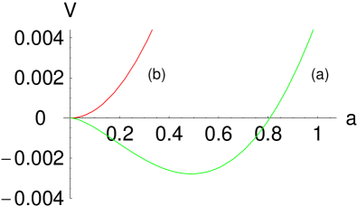
Figure 1: The effective potential of SU(2) QCD in the pure magnetic background. Here (a) is the effective potential and (b) is the classical potential.

The evaluation of the integral (24) for arbitrary $a$ and $b$ has been notoriously difficult savv ; niel ; ditt . Even in the case of “simpler” QED the integration of the effective action has been completed only recently cho01 ; cho5 . Fortunately the integral for the pure electric ($a=0$) and pure magnetic ($b=0$) background has now been correctly performed cho3 ; cho4 . For a pure monopole background (i.e., with $G_{\mu\nu}=H_{\mu\nu}$) we have $b=0$, so that the integral (24) becomes

$$\Delta{\cal L}=\displaystyle\frac{1}{16\pi^{2}}\int_{0}^{\infty}\displaystyle\frac{dt}{t^{2}}\displaystyle\frac{a/\mu^{2}}{\sinh(at/\mu^{2})}\Big{[}\exp(-2at/\mu^{2})+\exp(+2at/\mu^{2})\Big{]}.$$ (25)

To perform the integral we have to regularize the infra-red divergence first. For this we go to the Minkowski time with the Wick rotation, and find cho3 ; cho4

$$\Delta{\cal L}=\Delta{\cal L_{+}}+\Delta{\cal L_{-}},$$

$$\Delta{\cal L_{+}}=-\displaystyle\frac{1}{16\pi^{2}}\int_{0}^{\infty}\displaystyle\frac{dt}{t^{2}}\displaystyle\frac{a/\mu^{2}}{\sin(at/\mu^{2})}\exp(-2iat/\mu^{2}),$$

$$\Delta{\cal L_{-}}=-\displaystyle\frac{1}{16\pi^{2}}\int_{0}^{\infty}\displaystyle\frac{dt}{t^{2}}\displaystyle\frac{a/\mu^{2}}{\sin(at/\mu^{2})}\exp(+2iat/\mu^{2}).$$ (26)

In this form the infra-red divergence has disappeared, but now we face an ambiguity in choosing the correct contours of the integrals in (III). Fortunately this ambiguity can be resolved by causality. To see this notice that the two integrals $\Delta{\cal L_{+}}$ and $\Delta{\cal L_{-}}$ originate from the two determinants ${\rm Det}(-{\hat{D}}^{2}+2a)$ and ${\rm Det}(-{\hat{D}}^{2}-2a)$, and the standard causality argument requires us to identify $2a$ in the first determinant as $2a-i\epsilon$ but in the second determinant as $2a+i\epsilon$. This tells that the poles in the first integral in (III) should lie above the real axis, but the poles in the second integral should lie below the real axis. From this we conclude that the contour in $\Delta{\cal L_{+}}$ should pass below the real axis, but the contour in $\Delta{\cal L_{-}}$ should pass above the real axis. With this causality requirement the two integrals become complex conjugate to each other. This guarantees that $\Delta{\cal L}$ is explicitly real, without any imaginary part.

With this infra-red regularization by causality we obtain

$${\cal L}_{eff}=-\displaystyle\frac{a^{2}}{2g^{2}}-\displaystyle\frac{11}{48\pi^{2}}a^{2}(\ln\displaystyle\frac{a}{\mu^{2}}-c),$$

$$c=1-\ln 2-\displaystyle\frac{24}{11}\zeta^{\prime}(-1,\frac{3}{2})=0.94556...,$$ (27)

for a pure monopole background, where $\zeta(x,y)$ is the generalized Hurwitz zeta function cho3 ; cho4 .

For the pure electric background (i.e., with $a=0$) the infra-red regularization by causality gives us cho3 ; cho4

$${\cal L}_{eff}=\displaystyle\frac{b^{2}}{2g^{2}}+\displaystyle\frac{11b^{2}}{48\pi^{2}}(\ln\displaystyle\frac{b}{\mu^{2}}-c)-i\displaystyle\frac{11b^{2}}{96\pi}.$$ (28)

Observe that (III) and (28) are related by the duality. In fact we can obtain one from the other simply by replacing $a$ with $-ib$ and $b$ with $ia$. This duality, which states that the effective action should be invariant under the replacement

$$a\rightarrow-ib,~{}~{}~{}~{}~{}~{}~{}b\rightarrow ia,$$ (29)

was recently established as a fundamental symmetry of the effective action of gauge theory, both Abelian and non-Abelian cho3 ; cho01 . We emphasize that the duality provides a very useful tool to check the self-consistency of the effective action.

Remarkably the the effective action (27) generates the much desired dimensional transmutation in QCD, the phenomenon Coleman and Weinberg first observed in massless scalar QED cole . It is this dimensional transmutation that produces the dynamical generation of mass gap through the monopole condensation cho3 ; cho4 . To demonstrate this we first renormalize the effective action. Notice that the effective action (27) provides the following effective potential

$$V=\displaystyle\frac{1}{2}\displaystyle\frac{a^{2}}{g^{2}}\Big{[}1+\displaystyle\frac{11g^{2}}{24\pi^{2}}(\ln\displaystyle\frac{a}{\mu^{2}}-c)\Big{]}.$$ (30)

So we define the running coupling $\bar{g}$ by savv ; cho3

$$\frac{\partial^{2}V}{\partial a^{2}}\Big{|}_{a=\bar{\mu}^{2}}=\frac{1}{\bar{g}^{2}}.$$ (31)

With the definition we find

$$\frac{1}{\bar{g}^{2}}=\frac{1}{g^{2}}+\frac{11}{24\pi^{2}}(\ln\frac{{\bar{\mu}}^{2}}{\mu^{2}}-c+\displaystyle\frac{3}{2}),$$ (32)

from which we obtain the following $\beta$-function,

$$\beta(\bar{\mu})=\bar{\mu}\displaystyle\frac{\partial\bar{g}}{\partial\bar{\mu}}=-\frac{11}{24\pi^{2}}\bar{g}^{3}~{}.$$ (33)

This is exactly the same $\beta$-function that one obtained from the perturbative QCD to prove the asymptotic freedom wil . This confirms that our effective action is consistent with the asymptotic freedom.

The fact that the $\beta$-function obtained from the effective action becomes identical to the one obtained by the perturbative calculation is really remarkable, because this is not always the case. In fact in QED it has been demonstrated that the running coupling and the $\beta$-function obtained from the effective action is different from those obtained from the perturbative method cho3 ; cho5 .

In terms of the running coupling the renormalized potential is given by

$$V_{\rm ren}=\displaystyle\frac{1}{2}\displaystyle\frac{a^{2}}{\bar{g}^{2}}\Big{[}1+\displaystyle\frac{11}{24\pi^{2}}\bar{g}^{2}(\ln\displaystyle\frac{a}{\bar{\mu}^{2}}-\displaystyle\frac{3}{2})\Big{]},$$ (34)

which generates a non-trivial local minimum at

$$<a>=\bar{\mu}^{2}\exp\Big{(}-\frac{24\pi^{2}}{11\bar{g}^{2}}+1\Big{)}.$$ (35)

Notice that with ${\bar{\alpha}}_{s}=1$ we have

$$\displaystyle\frac{<a>}{{\bar{\mu}}^{2}}=0.48988....$$ (36)

This is nothing but the desired magnetic condensation. This proves that the one loop effective action of QCD in the presence of the constant magnetic background does generate a phase transition thorugh the monopole condensation cho3 ; cho4 .

The corresponding effective potential is plotted in Fig. 1, where we have assumed $\bar{\alpha}_{s}=1,~{}\bar{\mu}=1$. The effective potential clearly shows that there is indeed a dynamical generation of mass gap which indicates the existence of the confinement phase in QCD.

IV Stability of Monopole Condensation

The effective action of QCD in the presence of pure magnetic background (i.e., for $b=0$) has first been calculated by Savvidy and subsequently by Nielsen and Olesen savv ; niel . Their effective action was almost identical to ours, except that theirs contains the following extra imaginary part,

$${\rm Im}\thinspace{\cal L}_{eff}\Big{|}_{SNO}=~{}\displaystyle\frac{a^{2}}{8\pi}~{}~{}~{}~{}~{}~{}~{}b=0.$$ (37)

This sharply contradicts with our result (27) and (28), which has the following imaginary part,

$${\rm Im}~{}{\cal L}_{eff}=\left\{{~{}~{}~{}~{}0~{}~{}~{}~{}~{}~{}~{}~{}~{}~{}~{}~{}~{}~{}~{}b=0~{}~{}\atop-\displaystyle\frac{11b^{2}}{96\pi}~{}~{}~{}~{}~{}~{}~{}~{}~{}~{}~{}a=0~{}.}\right.$$ (38)

Clearly the imaginary part of the SNO effective action destabilizes our vacuum (35) through the pair creation of gluons. This would nullify our result, the monopole condensation and the dynamical generation of mass in QCD. So it becomes a most urgent issue to find out which of the effective actions is correct.

To settle thiss issue, one must understand the origin of the difference. The argument for the imaginary part in the SNO effective action was that the magnetic background should generate unstable tachyonic modes in the long distance region. These tachyonic modes, they argued, would generate an imaginary part to the effective action and render the vacuum condensation unstable. And indeed one does obtain (37), if one naively regularizes the infra-red divergence of the integral (25) with the $\zeta$-function regularization niel ; ditt .

Notice that these unstable modes, however, are unphysical which violate the causality. Furthermore, the SNO vacuum is not gauge invariant, and one can argue that the unstable modes originate from this fact. So one must be careful to exclude the unphysical modes when one regularizes the infra-red divergence. As we have pointed out, the infra-red regularization by causality naturally removes the unphysical modes and gives us the correct effective action. Furthermore, this regularization has been shown to preserve the duality, an important consistency condition for the effective actions in gauge theories cho3 ; cho4 .

Our infra-red regularization by causality assures the existence of the monopole condensation in $SU(2)$ QCD without doubt. On the other hand, since the $\zeta$-function regularization is also a well-established regularization method, it is not at all clear which regularization is the correct one for QCD at this moment. Given the fact that the stability of the vacuum condensation is such an important issue which can make or break the confinement, one must find an independent method to resolve the controversy. We now discuss a straightforward perturbative method to calculate the imaginary part of the effective action which can resolve the controversy and guarantee the stability of the monopole condensation. We present two independent methods based on the perturbative expansion, the Feynman diagram calculation and the perturbative calculation of the imaginary part of the effective action, to justify the infra-red regularization by causality.

V Imaginary Part of Effective Action in Massless QED

Before we discuss QCD we have to prove that one can indeed calculate the imaginary part of the effective action either perturbatively or non-perturbatively in massless gauge theories. As far as we understand, this has never been demonstrated before. So in this section we first calculate the imaginary part of the effective action of massless QED perturbatively, and show that the perturbative result is identical to the non-perturbative result.

The imaginary part of the non-perturbative one-loop effective action of QED has been known to be cho01 ; cho5 ,

$${\rm Im}\,{\cal L}_{QED}=\displaystyle\frac{ab}{8\pi^{2}}\sum_{n=1}^{\infty}\displaystyle\frac{1}{n}\coth\Big{(}\displaystyle\frac{n\pi a}{b}\Big{)}$$

$$\times\exp\Big{(}-\displaystyle\frac{n\pi m^{2}}{b}\Big{)},$$ (39)

where $m$ is the electron mass and

$$a=\displaystyle\frac{e}{2}\sqrt{\sqrt{F^{4}+(F\tilde{F})^{2}}+F^{2}},$$

$$b=\displaystyle\frac{e}{2}\sqrt{\sqrt{F^{4}+(F\tilde{F})^{2}}-F^{2}}.$$

In the massless limit this gives us cho01 ; cho5

$${\rm Im}\,{\cal L}_{QED}{\Big{|}}_{m=0}=\left\{{~{}0~{}~{}~{}~{}~{}~{}~{}~{}~{}~{}~{}~{}~{}~{}b=0~{}~{}\atop\displaystyle\frac{b^{2}}{48\pi}~{}~{}~{}~{}~{}~{}~{}~{}~{}~{}~{}a=0~{}.}\right.$$ (40)

Notice that the imaginary part is indeed of the order $e^{2}$, which is not the case when $m\neq 0$. We emphasize that the massless limit is well-defined because the one-loop effective action of massless QED has no infra-red divergence when $ab=0$ cho01 ; cho5 .

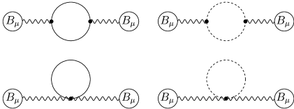
Figure 2: The Feynman diagrams that contribute to the effective action at $g^{2}$ order.

Now we calculate the imaginary part perturbatively to the order $e^{2}$. There are two different ways to do this, by calculating the Feynman diagram directly to the order $e^{2}$ or by making the perturbative expansion of the non-perturbative one-loop effective action. We start with the Feynman diagram. It is well-known that, to the order $e^{2}$, the electron loop diagram for an arbitrary background $A_{\mu}$ (with the dimensional regularization) gives us pesk

$$\displaystyle\frac{1}{2}\int d^{4}pA_{\mu}(p)\Pi_{\mu\nu}(p)A_{\nu}(-p)$$

$$=\displaystyle\frac{ie^{2}}{4\pi^{2}}\int d^{4}pA_{\mu}(p)(p^{2}g_{\mu\nu}-p_{\mu}p_{\nu})A_{\nu}(-p)$$

$$\times\displaystyle\frac{}{}\int_{0}^{1}dxx(1-x)\Big{(}-\displaystyle\frac{2}{\epsilon}+\gamma+\ln[1-x(1-x)\displaystyle\frac{p^{2}}{m^{2}}]\Big{)}$$

$$=\displaystyle\frac{ie^{2}}{8\pi^{2}}\int d^{4}pF_{\mu\nu}(p)F_{\mu\nu}(-p)\displaystyle\frac{}{}\int_{0}^{1}dxx(1-x)$$

$$\times\Big{(}-\displaystyle\frac{2}{\epsilon}+\gamma+\ln[1-x(1-x)\displaystyle\frac{p^{2}}{m^{2}}]\Big{)},$$ (41)

where $\Pi_{\mu\nu}(p)$ is the vacuum polarization tensor and $m$ is the electron mass. In the massless limit (with the subtraction of infra-red divergence at $\mu^{2}$) this gives us the leading contribution to the effective action

$$\Delta S_{QED}=\displaystyle\frac{e^{2}}{48\pi^{2}}\int d^{4}pF_{\mu\nu}(p)F_{\mu\nu}(-p)$$

$$\times\Big{[}\ln\Big{(}\displaystyle\frac{p^{2}}{\mu^{2}}\Big{)}+C_{0}\Big{]}$$ (42)

where $C_{0}$ is a regularization-dependent constant which can be absorbed to the wave function renormalization.

Clearly the imaginary part could only arise from the term $\mbox{ln}(p^{2}/\mu^{2})$, so that for a space-like $p^{2}$ (with $\mu^{2}>0$) the effective action has no imaginary part. But since a space-like $p^{2}$ corresponds to a magnetic background ($b=0$), we find that the magnetic condensation generates no imaginary part, at least at the order $e^{2}$.

As for the electric background ($a=0$) in general we need to consider a time-like $p^{2}$, but here we are interested in a constant electric background. In this case we have to go to the limit $p^{2}=0$ and make the analytic continuation of (42) to $p^{2}=0$. This is a delicate task. Fortunately the causality, with the familiar prescription $p^{2}\rightarrow p^{2}-i\epsilon$, guides us to make the analytic continuation correctly. Indeed the causality tells that

$$\displaystyle\frac{}{}\lim_{p^{2}\to 0}~{}\mbox{ln}\Big{(}\displaystyle\frac{p^{2}}{\mu^{2}}\Big{)}\rightarrow\lim_{p^{2}\to 0}~{}\mbox{ln}\Big{(}\displaystyle\frac{p^{2}}{\mu^{2}}-i\epsilon\Big{)}$$

$$=~{}\infty-i\displaystyle\frac{\pi}{2}.$$ (43)

From this we obtain (to the order $e^{2}$)

$${\rm Im}~{}{\cal L}_{QED}{\Big{|}}_{m=0}=\left\{{~{}0~{}~{}~{}~{}~{}~{}~{}~{}~{}~{}~{}~{}~{}~{}b=0,\atop\displaystyle\frac{b^{2}}{48\pi}~{}~{}~{}~{}~{}~{}~{}~{}~{}~{}~{}a=0,}\right.$$

which obviously is identical to the non-perturbative result (40).

Next, we calculate the imaginary part of the effective action of massless QED by making the perturbative expansion of the effective action to the order $e^{2}$. For this it is instructive for us to review Schwinger’s perturbative calculation of the QED effective action, who obtained schw

$$\Delta S_{QED}=\displaystyle\frac{e^{2}}{16\pi^{2}}\int d^{4}pF_{\mu\nu}(p)F_{\mu\nu}(-p)$$

$$\times\displaystyle\frac{}{}\int_{0}^{1}dv\displaystyle\frac{v^{2}(1-v^{2}/3)}{1-v^{2}+4m^{2}/p^{2}}.$$ (44)

Clearly the imaginary part can only arise when the integrand develops a pole, so that the effective action has no imaginary part when $p^{2}>-4m^{2}$. This confirms that, for the magnetic background, the QED effective action has no imaginary part.

But notice that when $p^{2}<-4m^{2}$ the integrand develops a pole at $v^{2}=1+4m^{2}/p^{2}$, and Schwinger taught us how to calculate the imaginary part of the effective action with the causality prescription $p^{2}\rightarrow p^{2}-i\epsilon$. But we notice that in the massless limit, the pole moves to $v=1$. In this case the pole contribution to the imaginary part is reduced by a half because only one quarter, not a half, of the pole contributes to the integral. With this observation we again reproduce (40) cho4 .

This proves that one can calculate the imaginary part of the effective action of massless QED perturbatively or non-perturbatively, with identical results. We emphasize that the perturbative calculation of the imaginary part of the effective action of massless QED has never been performed correctly before.

VI Diagrammatic Calculation of Imaginary Part of QCD Effective Action

A remarkable point of QCD is that the imaginary part of the one-loop effective action is of the order $g^{2}$. This is evident from both (37) and (38). This allows us to calculate the imaginary part perturbatively. In this section we calculate the imaginary part of the effective action of QCD perturbatively from Feynman diagrams. To do this we can either use the non-Abelian formalism or the Abelian formalism of QCD. Here we will use the latter in order to make the connection between QED and QCD more transparent.

For an arbitrary background $B_{\mu}$ there are four Feynman diagrams that contribute to the order $g^{2}$. They are shown schematically in Fig. 2. Here the straight line and the dotted line represent the valence gluon and the ghost, respectively. The tadpole diagrams contain a quadratic divergence which does not appear in the final result.

The sum of these diagrams is given (in Feynman gauge with dimensional regularization) by pesk

$$\displaystyle\frac{1}{2}\int d^{4}pB_{\mu}(p)\Pi_{\mu\nu}(p)B_{\nu}(-p)$$

$$=i\displaystyle\frac{11g^{2}}{96\pi^{2}}\int d^{4}pG_{\mu\nu}(p)G_{\mu\nu}(-p)\displaystyle\frac{}{}\int_{0}^{1}dxx(1-x)$$

$$\times\Big{(}-\displaystyle\frac{2}{\epsilon}+\gamma+\ln[1-x(1-x)\displaystyle\frac{p^{2}}{\mu^{2}}]\Big{)},$$ (45)

so that we have

$$\Delta S_{eff}=-\displaystyle\frac{11g^{2}}{96\pi^{2}}\displaystyle\int d^{4}pG_{\mu\nu}(p)G_{\mu\nu}(-p)$$

$$\times\left[\displaystyle\frac{2}{\epsilon}-\gamma-\mbox{ln}\left(\displaystyle\frac{p^{2}}{\mu^{2}}\right)\right].$$ (46)

Evidently the imaginary part can only arise from the term $\mbox{ln}(p^{2}/\mu^{2})$, and just as in massless QED we have no imaginary part for the monopole condensation (for $b=0$).

To evaluate the imaginary part for a constant electric background (for $a=0$) we have to make the analytic continuation of (46) to $p^{2}=0$. Here again the causality requirement (43) dictates how to make the analytic continuation, and we obtain

$${\rm Im}~{}\Delta{\cal L}=-\displaystyle\frac{11b^{2}}{96\pi}~{}~{}~{}~{}~{}~{}~{}~{}~{}(a=0).$$ (47)

So (46) gives us cho4

$${\rm Im}~{}{\cal L}_{eff}=\left\{{~{}~{}~{}~{}0~{}~{}~{}~{}~{}~{}~{}~{}~{}~{}~{}~{}~{}~{}~{}b=0~{}~{}\atop-\displaystyle\frac{11b^{2}}{96\pi}~{}~{}~{}~{}~{}~{}~{}~{}~{}~{}~{}a=0~{},}\right.$$

which is identical to (38). From this we conclude that indeed the Feynman diagram calculation of the imaginary part does produce the result which is identical to what we obtained from the one-loop effective action of QCD cho3 ; cho4 .

VII Schwinger’s Method

To remove any remaining doubt about the imaginary part (38) we now verify the above result by evaluating the functional determinant (23) of the effective action perturbatively to the order $g^{2}$. With our Abelian formalism of QCD, one can do this by following the method Schwinger used to evaluate the effective action of QED perturbatively step by step schw . This is presented in the Appendix. Here we do this in a slightly different way using a modern language, by calculating the functional determinant (23) to the order $g^{2}$.

To calculate the determinant we consider the determinant of the form

$${\rm Det}\,M = {\rm Det}\,(-{\hat{D}}^{2}+gR),$$ (48)

where $R=\pm 2a/g,\pm 2ib/g$, and $0$. We can rewrite

$${\rm Det}\,M={\rm Det}\,(-\partial^{2})\cdot{\rm Det}[1+\displaystyle\frac{1}{\partial^{2}}ig({\partial}_{\mu}B_{\mu}+B_{\mu}\partial_{\mu})$$

$$-\displaystyle\frac{1}{\partial^{2}}g^{2}B_{\mu}^{2}-\displaystyle\frac{1}{\partial^{2}}gR]$$

$$={\rm Det}\,(-\partial^{2})\cdot{\rm Det}[1+\Delta+\tilde{\Delta}+\hat{\Delta}],$$ (49)

and calculate the determinant by expanding it. At the lowest order in $g^{2}$ we have

$$\ln{\rm Det}M={\rm Tr}\ln M={\rm Tr}(\tilde{\Delta}-\displaystyle\frac{1}{2}\Delta^{2}-\displaystyle\frac{1}{2}\hat{\Delta}^{2}).$$ (50)

Now, using a standard technique pesk ; hon (with dimensional regularization) we obtain to the order $g^{2}$,

$${\rm Tr}\ln\,(-{\hat{D}}^{2}+gR)$$

$$=\displaystyle\frac{ig^{2}}{16\pi^{2}}\int d^{4}p\int_{0}^{1}dv\int_{0}^{\infty}\displaystyle\frac{dt}{t}\exp\Big{[}{-\displaystyle\frac{p^{2}}{4\mu^{2}}(1-v^{2})t}\Big{]}$$

$$\times\Big{[}\displaystyle\frac{v^{2}}{4}G_{\mu\nu}(p)G_{\mu\nu}(-p)-\displaystyle\frac{1}{2}R(p)R(-p)\Big{]}.$$ (51)

From this we find that the determinant (23) is given, up to the order $g^{2}$, by cho4

$$\Delta S=\displaystyle\frac{g^{2}}{8\pi^{2}}\int d^{4}pG_{\mu\nu}(p)G_{\mu\nu}(-p)\Sigma(p),$$

$$\Sigma(p)=\displaystyle\frac{}{}\int_{0}^{1}dv(1-\displaystyle\frac{v^{2}}{4})\displaystyle\frac{}{}\int_{0}^{\infty}\displaystyle\frac{dt}{t}\exp[-\displaystyle\frac{p^{2}}{4\mu^{2}}(1-v^{2})t]$$

$$=-2\displaystyle\frac{}{}\int_{0}^{1}dv\displaystyle\frac{v^{2}(1-v^{2}/12)}{1-v^{2}}+C_{1},$$ (52)

where $C_{1}$ is a regularization-dependent constant. Now, it is straightforward to evaluate the imaginary part of $\Delta S$, because the imaginary part can only arise from the pole at $v=1$. So repeating the argument to derive the imaginary part for massless QED in Section V, we again reproduce (38), after the proper wave function renormalization cho4 .

The fact that the Feynman diagram calculation and the Schwinger’s method produce an identical result is not accidental, because they are physically equivalent pesk . In fact, one can easily convince oneself that, order by order the perturbative expansion of the determinant (23) has one to one correspondence with the Feynman diagram expansion. And up to the order $g^{2}$, the Feynman diagrams that contribute to the determinant (23) are precisely those given by Fig. 2. Another way to see this is to notice that, from the definition of the exponential integral function table

$$Ei(-z)=-\displaystyle\frac{}{}\int_{z}^{\infty}\displaystyle\frac{d\tau}{\tau}\exp(-\tau)$$

$$=\gamma+\mbox{ln}z+\displaystyle\frac{}{}\int_{0}^{z}\displaystyle\frac{d\tau}{\tau}\left[\exp(-\tau)-1\right],~{}~{}({\rm Re}z>0)$$ (53)

we can express $\Sigma(p)$ in (52) by

$$\Sigma(p)=-\displaystyle\frac{}{}\lim_{\epsilon\to 0}\int_{0}^{1}dv(1-\displaystyle\frac{v^{2}}{4})\left[\gamma+\mbox{ln}\Big{(}\displaystyle\frac{p^{2}}{4\mu^{2}}(1-v^{2})\epsilon\Big{)}\right]$$

$$=-\displaystyle\frac{11}{12}\left[\mbox{ln}\left(\displaystyle\frac{p^{2}}{\mu^{2}}\right)+C_{2}\right],$$ (54)

where $C_{2}$ is another constant which can be removed by the wave function renormalization. But this is exactly what we had in (46) in the Feynmam diagram calculation (up to the irrelevant renormalization constant). This assures that the calculations of the imaginary part by Feynman diagram and by Schwinger’s method are indeed physically equivalent.

It must be emphasized again that, just as in the calculation of the non-perturbative effective action, the causality plays the crucial role in these perturbative calculations of the imaginary part of the effective action.

This confirms that the monopole condensation indeed describes a stable vacuum, but the electric background creates the pair-annihilation of the valence gluons in $SU(2)$ QCD cho3 ; cho4 . As importantly this confirms that the infra-red regularization by causality in the calculation of the effective action of QCD is indeed correct.

VIII Discussion

The proof of the monopole condensation in QCD has been extremely difficult to attain. The earlier attempts to calculate the effective action of QCD to prove the confinement have produced a negative result. In particular, the instability of the SNO vacuum has created a false impression that one can not prove the monopole condensation by calculating the effective action of QCD. The instability of the SNO vacuum can be traced back to the $\zeta$-function regularization of the infra-red divergence of the gluon loop integral (25). But we have recently pointed out that the $\zeta$-function regularization violates the causality, and proposed the infrared regularization by causality as the correct regularization in QCD. With the infrared regularization by causality we proved that a stable monopole condensation does take place at one loop level which can generate the dual Meissner effect and the confinement of color in $SU(2)$ QCD cho3 ; cho4 .

Considering the fact that the $\zeta$-function regularization is a well-established regularization method which has worked so well in other theories, however, one can not easily dismiss the instability of the SNO vacuum. Under this circumstance one definitely want to know which is the correct regularization in QCD, and why that is so.

In this paper we have checked the correctness of the infrared regularization by causality with two independent methods based on the perturbative expansion. Both methods produce a result identical to the one obtained with the infra-red regularization by causality, confirming the stability of the monopole condensation. This confirms that the magnetic confinement is indeed the correct confinement mechanism in QCD.

We emphasize that the above perturbative calculation of the imaginary part of the one-loop effective action was possible because in QCD (and in massless QED) the imaginary part of the one-loop effective action is of the order $g^{2}$ cho4 ; sch . This assures us that one can make a perturbative expansion for the imaginary part of the effective action. For massive QED, for example, this calculation does not make sense because the imaginary (as well as the real) part of the effective action simply does not allow a convergent perturbative expansion cho01 ; cho5 . The same argument applies to the real part of QCD. Only for the imaginary part of massless gauge theories one can make sense out of the perturbative calculation.

One might worry about the negative signature of the imaginary part in the QCD effective action. To understand the origin of this, compare QCD with QED. In QED we integrate the electron loop, and we know that the imaginary part of the effective action is positive cho01 ; schw . But in QCD we have the valence gluon loop, and obviously the electron and the valence gluon have opposite statistics. Furthermore one can easily convince oneself that the two loop integrals do not change the signature, due to the the similar nature of interactions. This means that the imaginary part of the effective action in QED and QCD should have opposite signature. This is the reason for the negative signature cho3 ; cho4 . We emphasize that this is what one should have expected from the asymptotic freedom. A positive imaginary part would make pair-creation, not pair-annhilation, of the valence gluons. This would produce the screenig, not the anti-screening, of the color charge. Obviously this is against the asymptotic freedom. This assures us that indeed the electric background generates pair-annihilation, not pair-creation, of gluons in QCD.

We have neglected the quarks in this paper. We simply remark that the quarks, just like in asymptotic freedom wil , tend to destabilize the monopole condensation. In fact the stability puts exactly the same constraint on the number of quarks as the asymptotic freedom cho6 . Furthermore here we have considered only the pure magnetic or pure electric background. So, to be precise, the above result only proves the existence of a stable monopole condensation for a pure magnetic background. To show that this is the true vacuum of QCD, one must calculate the effective action with an arbitrary background in the presence of the quarks and show that the monopole condensation remains a true minimum of the effective potential. Fortunately, one can actually calculate the effective action with an arbitrary constant background, and show that indeed the monopole condensation becomes the true vacuum of $SU(2)$ QCD, at least at one-loop level cho6 .

It is truly remarkable (and surprising) that the principles of quantum field theory allow us to demonstrate confinement within the framework of QCD. The failure to establish confinement within the framework of QCD has recently encouraged an increasing number of people to entertain the idea that a supersymmetric generalization of QCD might be necessary for confinement witt . Our analysis shows that this need not be the case. One can indeed demonstrate that QCD generates confinement by itself, with the existing principles of quantum field theory. This should be interpreted as a most spectacular triumph of quantum field theory itself.

Appendix

With the Abelian formalism of QCD, we can follow Schwinger step by step to obtain the imaginary part of the QCD effective action. For the pure magnetic case (i.e., for $b=0$), (23) is written as

$$\Delta S=i\mbox{Tr}~{}[\ln(-\hat{D}^{2}+2a)+\ln(-\hat{D}^{2}-2a)].$$ (55)

Using the identity

$$\ln M=-\int_{0}^{\infty}\displaystyle\frac{ds}{s}\exp(-iMs),$$ (56)

this can be expressed as

$$\Delta S = -i\mbox{Tr}\int_{0}^{\infty}\displaystyle\frac{ds}{s}[\exp(-i(\hat{D}^{2}-2a)s)$$ (57)

$$+\exp(-i(\hat{D}^{2}+2a)s)].$$

The perturbative expansion of

$$\mbox{Tr}~{}U(s)_{\pm}\equiv\mbox{Tr}\exp(-i(\hat{D}^{2}\mp 2a)s),$$ (58)

in powers of $g\tilde{C}_{\mu}$ and $a$ (remember that $a$ contains a factor of $g$) can be read from Schwinger’s work schw .

To second order in $g$ we have

$$\mbox{Tr}~{}U(s)_{\pm}=\mbox{Tr}U_{0}(s)-is\mbox{Tr}[{\mathcal{G}}_{\pm}U_{0}(s)]$$

$$-\displaystyle\frac{1}{2}s^{2}\int_{0}^{1}du\mbox{Tr}[{\mathcal{G}}_{\pm}U_{0}((1-u)s){\mathcal{G}}_{\pm}U_{0}(us)],$$ (59)

where

$$U_{0}(s)=\exp(i\partial^{2}s),$$

$${\mathcal{G}}_{\pm}=-\hat{D}^{2}+\partial^{2}\pm 2a.$$

Substituting these into (57) we have

$$\Delta S=-2i\displaystyle\int\displaystyle\frac{ds}{s}\Big{\{}\mbox{Tr}\Big{[}\exp(i\partial^{2}s)\Big{]}-is\mbox{Tr}\Big{[}g^{2}\tilde{C}_{\mu}^{2}\exp(i\partial^{2}s)\Big{]}$$

$$+g^{2}s^{2}\displaystyle\int^{1}_{-1}dv\mbox{Tr}\Big{[}\partial_{\mu}\tilde{C}_{\mu}\exp\Big{(}\displaystyle\frac{i}{2}\partial^{2}(1-v)s\Big{)}\partial_{\mu}\tilde{C}_{\mu}\exp\Big{(}\displaystyle\frac{i}{2}\partial^{2}(1+v)s\Big{)}\Big{]}$$

$$-a^{2}s^{2}\displaystyle\int^{1}_{-1}dv\mbox{Tr}\Big{[}\exp\Big{(}\displaystyle\frac{i}{2}\partial^{2}(1-v)s\Big{)}\exp\Big{(}\displaystyle\frac{i}{2}\partial^{2}(1+v)s\Big{)}\Big{]}\Big{\}},$$ (60)

where $u=(1+v)/2$. The next step is to take the trace, yielding

$$\Delta S=-2i\displaystyle\int\displaystyle\frac{ds}{s}\int d^{4}p\int\displaystyle\frac{d^{4}k}{(2\pi)^{4}}\Big{\{}\mbox{Tr}\Big{[}\exp(-ik^{2}s)\Big{]}-is\mbox{Tr}\Big{[}g^{2}\tilde{C}_{\mu}^{2}\exp(-ik^{2}s)\Big{]}$$

$$-\displaystyle g^{2}s^{2}\int^{1}_{-1}dv\mbox{Tr}\Big{[}k_{\mu}\tilde{C}_{\mu}\exp\Big{(}-\displaystyle\frac{i}{2}\Big{(}k+\displaystyle\frac{p}{2}\Big{)}^{2}(1-v)s\Big{)}k_{\mu}\tilde{C}_{\mu}\exp\Big{(}-\displaystyle\frac{i}{2}\Big{(}k-\displaystyle\frac{p}{2}\Big{)}^{2}(1+v)s\Big{)}\Big{]}$$

$$-a^{2}s^{2}\displaystyle\int^{1}_{-1}dv\mbox{Tr}\Big{[}\exp\Big{(}-\displaystyle\frac{i}{2}\Big{(}k+\displaystyle\frac{p}{2}\Big{)}^{2}(1-v)s\Big{)}\exp\Big{(}-\displaystyle\frac{i}{2}\Big{(}k-\displaystyle\frac{p}{2}\Big{)}^{2}(1+v)s\Big{)}\Big{]}\Big{\}}.$$ (61)

Following Schwinger’s technique and keeping only nonvanishing field-dependent terms, we obtain

$$\Delta S=\displaystyle\frac{a^{2}}{4\pi^{2}}\displaystyle\int\displaystyle\frac{ds}{s}\int d^{4}p\displaystyle\int_{0}^{1}dv\left(1-\displaystyle\frac{v^{2}}{4}\right)\exp\left(-\displaystyle\frac{i}{4}p^{2}(1-v^{2})s\right).$$ (62)

Now, with the Wick rotation $s\rightarrow-is$ and the integration by parts with respect to $v$, we have

$$\Delta S=\displaystyle\frac{a^{2}}{8\pi^{2}}\int d^{4}p\int\displaystyle\frac{ds}{s}\Big{\{}\displaystyle\frac{11}{6}+sp^{2}\displaystyle\int_{0}^{1}dvv^{2}\Big{(}1-\displaystyle\frac{v^{2}}{12}\Big{)}\exp\Big{(}-\displaystyle\frac{p^{2}}{4}(1-v^{2})s\Big{)}\Big{\}}$$

The first term in the square bracket has no imaginary part and is removed by renormalization. The second term is integrated over $s$ to yield

$$\Delta S=-\displaystyle\frac{a^{2}}{2\pi^{2}}\int d^{4}p\int_{0}^{1}dv\displaystyle\frac{v^{2}(1-v^{2}/12)}{1-v^{2}}.$$ (63)

On the other hand for the pure electric background (i.e., for $a=0$), we have

$$\Delta S=i\mbox{Tr}~{}[\ln(-\tilde{D}^{2}+2ib)+\ln(-\tilde{D}^{2}-2ib)],$$ (64)

Repeating the steps that lead to (63) we find

$$\Delta S=\displaystyle\frac{b^{2}}{2\pi^{2}}\int d^{4}p\int_{0}^{1}dv\displaystyle\frac{v^{2}(1-v^{2}/12)}{1-v^{2}}.$$ (65)

So, for an arbitrary background, we have

$$\Delta S=-\displaystyle\frac{a^{2}-b^{2}}{2\pi^{2}}\int d^{4}p\int_{0}^{1}dv\displaystyle\frac{v^{2}(1-v^{2}/12)}{1-v^{2}}.$$

This is identical to (52), again up to the irrelevant renormalization constant. This, with the argument in Sections VI and VII, confirms that the Schwinger’s method reproduces (38).

Acknowledgements

One of the authors (YMC) thanks S. Adler and F. Dyson for the fruitful discussions, and Professor C. N. Yang for the continuous encouragements. The other (DGP) thanks Professor C. N. Yang for the fellowship at Asia Pacific Center for Theoretical Physics, and appreciates Haewon Lee for numerous discussions. The work is supported in part by Korea Research Foundation (Grant KRF-2001 -015-BP0085) and by the BK21 project of Ministry of Education.

References

- (1) Y. Nambu, Phys. Rev. D10, 4262 (1974); S. Mandelstam, Phys. Rep. 23C, 245 (1976); A. Polyakov, Nucl. Phys. B120, 429 (1977); G. ’t Hooft, Nucl. Phys. B190, 455 (1981).
- (2) Y. M. Cho, Phys. Rev. D21, 1080 (1980); J. Korean Phys. Soc. 17, 266 (1984); Phys. Rev. D62, 074009 (2000).
- (3) Y. M. Cho, Phys. Rev. Lett. 46, 302 (1981); Phys. Rev. D23, 2415 (1981); W. S. Bae, Y. M. Cho, and S. W. Kimm, Phys. Rev. D65, 025005 (2002).
- (4) G. K. Savvidy, Phys. Lett. B71, 133 (1977).
- (5) N. Nielsen and P. Olesen, Nucl. Phys. B144, 485 (1978); C. Rajiadakos, Phys. Lett. B100, 471 (1981).
- (6) A. Yildiz and P. Cox, Phys. Rev. D21, 1095 (1980); M. Claudson, A. Yilditz, and P. Cox, Phys. Rev. D22, 2022 (1980); S. Adler, Phys. Rev. D23, 2905 (1981); W. Dittrich and M. Reuter, Phys. Lett. B128, 321, (1983); B144, 99 (1984); C. Flory, Phys. Rev. D28, 1425 (1983); S. K. Blau, M. Visser, and A. Wipf, Int. J. Mod. Phys. A6, 5409 (1991); M. Reuter, M. G. Schmidt, and C. Schubert, Ann. Phys. 259, 313 (1997).
- (7) Y. M. Cho, H. W. Lee, and D. G. Pak, Phys. Lett. B 525, 347 (2002); Y. M. Cho and D. G. Pak, Phys. Rev. D65, 074027 (2002).
- (8) Y. M. Cho and M. L. Walker, hep-th/0206127.
- (9) S. Coleman and E. Weinberg, Phys. Rev. D7, 1888 (1973).
- (10) Y. M. Cho and D. G. Pak, Phys. Rev. Lett. 86, 1947 (2001); W. S. Bae, Y. M. Cho, and D. G. Pak, Phys. Rev. D64, 017303 (2001). There is a typological mistake in the first paper, where the right hand side of Eq. (24) should have an overall minus sign.
- (11) Y. M. Cho and D. G. Pak, hep-th/0010073, submitted to Phys. Rev. D, Rapid Communication.
- (12) V. Schanbacher, Phys. Rev. D26, 489 (1982); L. Freyhult, hep-th/0106239.
- (13) J. Schwinger, Phys. Rev. 82, 664 (1951).
- (14) L. Faddeev and A. Niemi, Phys. Rev. Lett. 82, 1624 (1999); Phys. Lett. B449, 214 (1999).
- (15) S. Shabanov, Phys. Lett. B458, 322 (1999); B463, 263 (1999); H. Gies, Phys. Rev. D63, 125023 (2001).
- (16) T. T. Wu and C. N. Yang, Phys. Rev. D12, 3845 (1975).
- (17) Y. M. Cho, Phys. Rev. Lett. 44, 1115 (1980); Phys. Lett. B115, 125 (1982).
- (18) A. Belavin, A. Polyakov, A. Schwartz, and Y. Tyupkin, Phys. Lett. B59, 85 (1975); G. ’t Hooft, Phys. Rev. Lett. 37, 8 (1976).
- (19) Y. M. Cho, Phys. Lett. B81, 25 (1979).
- (20) B. de Witt, Phys. Rev. 162, 1195 (1967); 1239 (1967).
- (21) See for example, C. Itzikson and J. Zuber, Quantum Field Theory (McGraw-Hill) 1985; M. Peskin and D. Schroeder, An Introduction to Quantum Field Theory (Addison-Wesley) 1995; S. Weinberg, Quantum Theory of Fields (Cambridge Univ. Press) 1996.
- (22) D. Gross anf F. Wilczek, Phys. Rev. Lett. 26, 1343 (1973); H. Politzer, Phys. Rev. Lett. 26, 1346 (1973).
- (23) A similar calculation has first been carried out by Honerkamp. See, J. Honerkamp, Nucl. Phys. B48, 269 (1972).
- (24) See, for example, I. Gradshteyn and I. Ryzhik, Table of Integrals, Series, and Products, edited by A. Jeffery (Academic Press) 1994; M. Abramowitz and I. Stegun, Handbook of Mathematical Functions, (Dover) 1970.
- (25) Y. M. Cho and D. G. Pak, hep-th/0006051, submitted to Phys. Rev. D. See also Y. M. Cho and D. G. Pak, in Proceedings of TMU-Yale Symposium on Dynamics of Gauge Fields, edited by T. Appelquist and H. Minakata (Universal Academy Press, Tokyo) (1999).
- (26) N. Seiberg and E. Witten, Nucl. Phys. B426, 19 (1994); B431, 484 (1994).