Thermodynamics of a Kerr Newman de Sitter black hole

Abstract

We compute the conserved quantities of the four-dimensional Kerr-Newman-dS (KNdS) black hole through the use of the counterterm renormalization method, and obtain a generalized Smarr formula for the mass as a function of the entropy, the angular momentum and the electric charge. The first law of thermodynamics associated to the cosmological horizon of KNdS is also investigated. Using the minimal number of intrinsic boundary counterterms, we consider the quasilocal thermodynamics of asymptotic de Sitter Reissner-Nordstrom black hole, and find that the temperature is equal to the product of the surface gravity (divided by $2\pi$) and the Tolman redshift factor. We also perform a quasilocal stability analysis by computing the determinant of Hessian matrix of the energy with respect to its thermodynamic variables in both the canonical and the grand-canonical ensembles and obtain a complete set of phase diagrams. We then turn to the quasilocal thermodynamics of four-dimensional Kerr-Newman-de Sitter black hole for virtually all possible values of the mass, the rotation and the charge parameters that leave the quasilocal boundary inside the cosmological event horizon, and perform a quasilocal stability analysis of KNdS black hole.

PACS numbers: 04.70.Dy, 04.62.+v, 04.60.-m

I Introduction

The observational evidence for a positive cosmological constant and the proposed de Sitter conformal field theory (dS/CFT) correspondence Str1 have provided motivations for studying the thermodynamics of de Sitter spacetime in the presence of black holes Cai . Since asymptotic de Sitter black holes have a cosmological event horizon, one may use a local description of thermodynamics of the event or cosmological horizons separately Pad . Another way of studying the thermodynamics of these kind of black holes is to investigate their quasilocal thermodynamics Deh .

One of the quantities associated with the gravitational thermodynamics of black holes is the physical entropy $S$ which is proportional to the area of the event horizon(s) Beck ; Haw . The surprising and impressive features of the area law of entropy is its universality which applies to all kinds of black holes and black strings HHP ; Mann , and it also applies to the cosmological event horizon of the asymptotic de Sitter black holes GH1 . Another quantity of interest is the temperature $\beta^{-1}$, which is proportional to the surface gravity of the event horizon(s).

Other black hole properties such as energy, angular momentum and conserved charges, can also be given a thermodynamic interpretation GH2 . But as is known, these quantities typically diverge for asymptotic flat, AdS, and dS spacetimes. A common approach of evaluating them has been to carry out all computations relative to some reference spacetime that is regarded as the ground state for the class of spacetimes of interest BY . Unfortunately, it suffers from several drawbacks. The choice of reference spacetime is not always unique CCM , nor is it always possible to embed a boundary with a given induced metric into the reference background. Indeed, for rotating spacetimes this latter problem creates a serious barrier against calculating the subtraction energy, and calculations have only been performed in the slow-rotating regime Mart . An extension of this approach that addresses these difficulties was developed based on the conjectured AdS/CFT correspondence for asymptotic AdS spacetimes Hen ; BK ; EJM , and recently for asymptotic de Sitter spacetimes Bal1 ; GM1 ; Deh1 . Indeed, the near-boundary analysis of asymptotically AdS spacetimes can be analytically continued to asymptotic dS spacetimes and therefore the counterterms have a straightforward continuation. It is believed that appending a counterterm, $I_{ct}$, to the action which depends only on the intrinsic geometry of the boundary(ies) can remove the divergences. This requirement, along with general covariance, implies that these terms are functionals of curvature invariants of the induced metric and have no dependence on the extrinsic curvature of the boundary(ies). An algorithmic procedure exists for constructing $I_{ct}$ for asymptotic AdS KLS and dS spacetimes GM1 , and so its determination is unique. Addition of $I_{ct}$ will not affect the bulk equations of motion, thereby eliminating the need to embed the given geometry in a reference spacetime. Hence thermodynamic and conserved quantities can now be calculated intrinsic for any given asymptotically AdS or dS spacetime. The efficiency of this approach has been demonstrated in a broad range of examples for both the asymptotic AdS and dS spacetimes Bal1 ; DaM ; GM1 ; Deh2 ; Deh3 .

Recently, we have considered the effects of including $I_{ct}$ for quasilocal gravitational thermodynamics of Kerr, Kerr-AdS and Kerr-dS black holes in which the region enclosed by $\partial\mathcal{M}$ was spatially finite. We have also performed a quasilocal stability analysis and found phase behavior that was incommensurate with their previous analysis carried out at infinity Deh ; Deh4 . In this paper, we investigate the thermodynamic properties of the class of Kerr-Newman-dS black holes in the context of both temporally infinite and spatially finite boundaries with the boundary action supplemented by $I_{ct}$. With their lower degree of symmetry relative to spherically symmetric black holes, these spacetimes allow for a more detailed study of the consequences of including $I_{ct}$ for temporally infinite and spatially finite boundaries. There are several reasons for considering this. First, one can obtain the thermodynamic quantities corresponding to an asymptotically de Sitter spacetime within a fixed radius, while there is no self-consistent thermodynamics for the whole spacetime. Furthermore, the inclusion of $I_{ct}$ eliminates the embedding problem from consideration, whether or not the temporary infinite limit is taken, and so it is of interest to see what its impact is on quasilocal thermodynamics.

The outline of our paper is as follows. We review the basic formalism in Sec. II. In Sec. III we consider the Kerr-Newman-dS₄ spacetime and compute the thermodynamic quantities associated to the cosmological horizon. Also we give a generalized Smarr formula and investigate the first law of thermodynamics for the cosmological event horizon. In Sec. IV, we consider the quasilocal thermodynamics of Reissner-Nordstrum-dS spacetime, and perform a stability analysis through the use of the determinant of Hessian matrix of the energy with respect to the entropy and the charge. In Sec. V, we compute the determinant of Hessian matrix of the energy with respect to its thermodynamic variables for Kerr-Newman-de Sitter black holes, numerically, and present our results graphically. We finish our paper with some concluding remarks.

II General Formalism

The gravitational action of four-dimensional asymptotically de Sitter spacetimes $\mathcal{M}$, with boundary $\mathcal{\delta M}^{\pm}$ in the presence of an electromagnetic field is

$$I_{G}=-\frac{1}{16\pi}\int_{\mathcal{M}}d^{4}x\sqrt{-g}\left(\mathcal{R}-2\Lambda-F_{\mu\nu}F^{\mu\nu}\right)+\frac{1}{8\pi}\int_{\mathcal{\delta M}^{-}}^{\mathcal{\delta M}^{+}}d^{3}x\sqrt{-\gamma}\Theta(\gamma),$$ (1)

where $F_{\mu\nu}=\partial_{\mu}A_{\nu}-\partial_{\nu}A_{\mu}$ is the electromagnetic tensor field and $A_{\mu}$ is the vector potential. In Eq. (1) $\mathcal{M}$ is the bulk manifold with metric $g_{\mu\nu}$, and $\mathcal{\delta M}^{\pm}$ are spacial boundaries at early and late times with induced metrics $\gamma_{ij}$ and the extrinsic curvature $\Theta^{\mu\nu}$. The first term is the Einstein-Maxwell term with positive cosmological constant $\Lambda=3/l^{2}$, and the second term is the Gibbons-Hawking boundary term that is chosen such that the variational principle is well defined. The notation $\int_{\mathcal{\delta M}^{-}}^{\mathcal{\delta M}^{+}}$ indicates an integral over the late-time boundary minus the integral over the early-time boundary which are both Euclidean denoted by $\mathcal{I}^{+}$ and $\mathcal{I}^{-}$ respectively. In general, $I_{G}$ of Eq. (1) is divergent when evaluated on the solutions at $\mathcal{I}^{\pm}$, as is the Hamiltonian and other associated conserved quantities. Rather than eliminating these divergences by incorporating a reference term in the spacetime, a new term $I_{ct}$ is added to the action that is a functional only of boundary curvature invariants Bal1 ; Deh1 . Although there may exist a very large number of possible invariants, one could add only a finite number of them in a given dimension. Quantities such as energy, mass, etc. can then be understood as intrinsically defined for a given spacetime, as opposed to being defined relative to some abstract (and non-unique) background, although this latter option is still available. In four dimensions the counterterm is Bal1

$$I_{ct}=\frac{2}{l}\frac{1}{8\pi}\int_{\mathcal{\delta M}^{\pm}}d^{3}x\sqrt{-\gamma}\left(1-\frac{l^{2}}{4}R\right),$$ (2)

where $R$ is the Ricci scalar of the boundary metric $\gamma_{ij}$ and $\int_{\mathcal{\delta M}^{\pm}}$ indicates the sum of the integral over the early and late time boundaries. Although other counterterms (of higher mass dimension) may be added to $I_{ct}$, they will make no contribution to the evaluation of the action or Hamiltonian due to the rate at which they decrease toward infinity, and we shall not consider them in our analysis here. It is worthwhile to mentioning that the inclusion of matter fields in the gravitational action requires the addition of further counterterms when the dimension of the bulk is greater than four. But since we consider the four-dimensional spacetimes, we don’t need any additional counterterms Sken2 .

A thorough discussion of the quasilocal formalism has been given elsewhere BY and so we only briefly recapitulate it here. The total action can be written as a linear combination of the gravity term (1) and the counterterms (2) as

$$I=I_{G}+I_{ct}.$$ (3)

Using the Brown and York definition BY one can construct a divergence-free stress-energy tensor from the total action (3) either on an early or late boundary as Bal1 :

$$T^{+ab} = -\frac{1}{8\pi}\left\{(\Theta^{ab}-\Theta\gamma^{ab})-\frac{2}{l}\left[\gamma^{ab}+\frac{l^{2}}{2}\left(R^{ab}-\frac{1}{2}R\gamma^{ab}\right)\right]\right\},$$ (4)

$$T^{-ab} = -\frac{1}{8\pi}\left\{-(\Theta^{ab}-\Theta\gamma^{ab})-\frac{2}{l}\left[\gamma^{ab}+\frac{l^{2}}{2}\left(R^{ab}-\frac{1}{2}R\gamma^{ab}\right)\right]\right\}.$$ (5)

To obtain the boundary stress tensor, we should evaluate Eq. (4) at fixed time and send time to infinity. We will suppress the $+$ sign notation in $T^{+ab}$ in the rest of the paper. To compute the thermodynamic and conserved quantities of the spacetime, one should write the metric $\gamma_{ab}$ on equal time surfaces in the ADM form:

$$\gamma_{ab}dx^{a}dx^{b}=N^{2}d\rho^{2}+\sigma_{ij}\left(d\phi^{i}+V^{i}d\rho\right)\left(d\phi^{j}+V^{j}d\rho\right),$$

where the coordinates $\phi^{i}$ are the angular variables parameterizing the closed surfaces around an origin. Then the total thermodynamic energy of the system is BY

$$E=\int_{\mathcal{B}}d^{2}\phi\sqrt{\sigma}\varepsilon;\hskip 28.45274pt\varepsilon=T_{ab}u^{a}u^{b},$$ (6)

where $u^{a}$ is the unit normal vector on a surface of fixed $\rho$ and $\sigma$ is the determinant of the metric $\sigma_{ij}$. If the boundary of the spacetime has an isometry generated by a Killing vector $\mathcal{\xi}^{a}$, then the conserved charge associated with $\mathcal{\xi}^{a}$ is Bal1

$$\mathcal{Q}(\mathcal{\xi)}=\int_{\mathcal{B}}d^{2}\phi\sqrt{\sigma}T_{ab}u^{a}\mathcal{\xi}^{b},$$ (7)

Since all the asymptotic de Sitter spacetimes have an asymptotic isometry generated by $\partial/\partial t$, there is a notion of a conserved mass as computed at future infinity as

$$M=\int_{\mathcal{B}}d^{2}\phi\sqrt{\sigma}T_{ab}u^{a}\xi^{b},$$ (8)

We compute the quantities of Eqs. (8) on a surface of fixed time and then send time to infinity so that it approaches the spacetime boundary at $\mathcal{I}^{\pm}$. Indeed, for $r$ greater than the radius of the cosmological horizon $t$ is a spatial direction, while $r$ will become a temporal coordinate. Thus, the large $r$ surfaces approach $\mathcal{I}^{\pm}$, and since we purpose to define the stress tensor, and the mass at $\mathcal{I}^{\pm}$, we will evaluate these quantities on the surface of large $r$.

Similarly if the surface $\mathcal{B}$ has an isometry generated by $\zeta=\partial/\partial\phi$, then the quantity

$$J=\int_{\mathcal{B}}d^{2}\phi\sqrt{\sigma}T_{ab}u^{a}\zeta^{b},$$ (9)

can be regarded as a conserved angular momentum associated with the surface $\mathcal{B}$. Many authors have used the counterterm method for various asymptotic de Sitter spacetimes and computed the associated conserved charges Bal1 ; GM1 ; Deh1 . We shall also study the implications of including the counterterms (2) for Reissner-Nordstrom-dS and Kerr-Newman-dS black holes in spatially finite region.

III The Thermodynamics associated to the cosmological horizon of the Kerr-Newman-dS₄ black hole

Here we consider the charged rotating black holes in four dimensions, whose general form is

$$ds^{2} = -\frac{\Delta_{r}^{2}}{\rho^{2}}\left(dt-\frac{a}{\Xi}\sin^{2}\theta d\phi\right)^{2}+\frac{\rho^{2}}{\Delta_{r}^{2}}dr^{2}$$ (10)

$$\ +\frac{\rho^{2}}{\Delta_{\theta}}d\theta^{2}+\frac{\Delta_{\theta}\sin^{2}\theta}{\rho^{2}}\left(adt-\frac{(r^{2}+a^{2})}{\Xi}d\phi\right)^{2},$$

where

$$\Delta_{r}^{2} = (r^{2}+a^{2})(1-r^{2}/l^{2})-2mr+q^{2},$$

$$\Delta_{\theta} = 1+\frac{a^{2}}{l^{2}}\cos^{2}\theta,$$

$$\Xi = 1+\frac{a^{2}}{l^{2}},$$

$$\rho^{2} = r^{2}+a^{2}\cos^{2}\theta,$$ (11)

and the vector potential $A_{\mu}$ is:

$$A_{\mu}=-\frac{qr}{\rho^{2}}(\delta_{\mu}^{t}-\frac{a\sin^{2}\theta}{\Xi}\delta_{\mu}^{\phi}).$$ (12)

For $q=0$, the metric (10) and (11) is Kerr-dS₄ spacetime (or Kerr spacetime if $l\rightarrow\infty$), and for $a=0$ the metric is Reissner Nordstrom-dS₄ spacetime, which has zero angular momentum. Here the parameters $m$, $a$, and $q$ are associated with the mass, the angular momentum and the charge of the spacetime, respectively. The metric of Eqs. (10) and (11) has three horizons located at $r_{-}$, $r_{+}$, and $r_{c}$, provided the parameters $m$, $l$, $a$, and $q$ are chosen suitably. The three parameters $l$, $a$ and $q$ should be chosen such that $l^{4}+a^{4}-14a^{2}l^{2}-12q^{2}l^{2}\geq 0$, and $m$ should lie in the range between $m_{1\hbox{\small{crit}}}\leq m\leq m_{2\hbox{\small{crit}}}$, where $m_{1\hbox{\small{crit}}}$ and $m_{2\hbox{\small{crit}}}$ are the positive real solutions of the following equation:

$$27l^{6}m^{4}+(33l^{4}a^{4}-36l^{6}q^{2}-33l^{6}a^{2}+36l^{4}q^{2}a^{2}+l^{2}a^{6}-l^{8})m^{2}$$

$$+a^{8}q^{2}+22l^{4}a^{4}q^{2}+12l^{6}a^{2}q^{2}+6a^{6}l^{4}+4l^{6}a^{4}+32l^{4}a^{2}q^{4}+l^{8}q^{2}$$

$$+12a^{6}l^{2}q^{2}+4l^{2}a^{8}+l^{8}a^{2}+a^{10}+16l^{4}q^{6}+8l^{6}q^{4}+8l^{2}q^{4}a^{4}=0.$$ (13)

It is worthwhile to mention that when $m=m_{1\hbox{\small{crit}}}$, $r_{-}$ and $r_{+}$ are equal and we have an extreme black hole. For the case in which $m=m_{2\hbox{\small{crit}}}$, the radii of event and cosmological horizons are equal and we have a critical hole. Also, one may note that in the limit $l\rightarrow\infty$, $m_{1\hbox{\small{crit}}}=\sqrt{a^{2}+q^{2}}$, $m_{2\hbox{\small{crit}}}\rightarrow\infty$, $r_{\pm}=m\pm\sqrt{m^{2}-a^{2}-q^{2}}$, and $r_{c}\rightarrow\infty$.

For given values of $a$ and $m$, the parameter $l$ should be greater than $l_{\hbox{\small{crit}}}$, where $l_{\hbox{\small{crit}}}$ is the positive real solution of Eq. (13). When $l=l_{\hbox{\small{crit}}}$, we have a critical hole. Also the positive real solution of Eq. (13) for $a$ gives the critical value of $a$ (upper bound for $a$) for which the hole is extremal. The two real solutions of Eq. (13) for $q$ determine the lower and upper bounds of $q$ that belong to the critical and extremal black hole, respectively.

Since the temperature associated with the event or cosmological horizons has different values for asymptotic de Sitter spacetimes one should use a local description of the thermodynamics of the black hole. In the remain of this section we investigate the thermodynamics associated to the cosmological horizon and in the next section we investigate the thermodynamic quantities associated with the spacetime within an arbitrary surface with fixed radius $r$.

Analytical continuation of the Lorentzian metric by $t\rightarrow i\tau$ and $a\rightarrow ia$ yields the Euclidean section, whose regularity at $r=r_{c}$ requires that we should identify $(\tau,\phi)\sim(\tau+\beta_{c},\phi+i\beta_{c}\Omega_{c})$, where $\beta_{c}$ and $\Omega_{c}$ are the inverse Hawking temperature and the angular velocity of the cosmological event horizon given as GH1 :

$$\beta_{c}=\frac{4\pi l^{2}r_{c}(r_{c}^{2}+a^{2})}{3r_{c}^{4}+a^{2}r_{c}^{2}-l^{2}r_{c}^{2}+a^{2}l^{2}+q^{2}l^{2}},$$ (14)

$$\Omega_{c}=\frac{a\Xi}{r_{c}^{2}+a^{2}}.$$ (15)

Since the area law of the entropy is universal, and it can be used for the cosmological horizon of dS black holes GH1 , the entropy is

$$S=\frac{\mathcal{A}_{c}}{4}=\frac{\pi(r_{c}^{2}+a^{2})}{\Xi}.$$ (16)

As we discussed in Sec. II, one can compute the finite action through the use of boundary counterterms. To do this one should take a space-like hypersurface, $\mathcal{P}$ of large constant $r$ ($r_{c}<r<\infty$) in the future and calculate the total action (3). In the limit that $r$ tends to infinity, this surface tends to future infinity $\mathcal{I}^{+}$ as expected. The first integral of the action in (1) should be first computed from $r_{c}$ to $r$, and then the total action should be integrated on the hypersurface $\mathcal{P}$. Sending $r$ to infinity the total action of the system is :

$$I=-\beta_{c}\frac{(r_{c}^{2}+a^{2})(r_{c}^{3}+r_{c}a^{2}+ml^{2})-r_{c}l^{2}q^{2}}{2l^{2}\Xi(r_{c}^{2}+a^{2})},$$ (17)

where $r_{c}$ and $\beta_{c}$ are the radius and the inverse of the Hawking temperature of the cosmological event horizon. The total mass can be calculated through the use of Eq. (8) and sending the temporal coordinate to infinity. We obtain

$$M=-\frac{m}{\Xi^{2}}.$$ (18)

It is worthwhile to note that as $a$ and $q$ go to zero, the action and mass given by Eqs. (17) and (18) reduce to those of Schwarzschild-dS black hole obtained in Bal1 . The total angular momentum can be computed through the use of Eq. (9) for a boundary with finite radius, $r_{+}<r<r_{c}$. It is a matter of calculation to show that $J$ is independent of $r$ given as:

$$J=-\frac{ma}{\Xi^{2}}.$$ (19)

We now obtain the mass as a function of the extensive quantities $S$, $J$ and $Q$, where $Q$ defined as $q/\Xi$. Using the expressions (18) and (16) for the mass, the angular momentum and the entropy, and the fact that $\Delta_{r}(r_{c})=0$, one can obtain a generalized Smarr formula as

$$M=-\left\{\frac{S}{4\pi}+\frac{\pi}{4S}(4J^{2}+Q^{4})+\frac{Q^{2}}{2}-\frac{J^{2}}{l^{2}}-\frac{S}{2\pi l^{2}}\left(Q^{2}+\frac{S}{\pi}-\frac{S^{2}}{2\pi l^{2}}\right)\right\}^{1/2}.$$ (20)

It is worthwhile to mentioning that the analytic continuation $l\rightarrow il$ (Wick rotates) changes the above Smarr formula to the Smarr formula of the Kerr-Newman-AdS black hole given in Ref. Cal Now, one may regard the parameters $S$, $J$ and $Q$ as a complete set of extensive parameters for the mass $M(S,J,Q)$ and define the intensive parameters conjugate to $S$, $J$ and $Q$. These quantities are the temperature, the angular velocities, and the electric potential defined as

$$T=\left(\frac{\partial M}{\partial S}\right)_{J,Q},\ \ \Omega=\left(\frac{\partial M}{\partial J}\right)_{S,Q},\ \ \Phi=\left(\frac{\partial M}{\partial Q}\right)_{S,J}.$$ (21)

It is a matter of straightforward calculation to show that the temperature calculated from Eq. (21) coincides with Eq. (14), and the angular velocity obtained from Eq. (21) is the thermodynamic angular velocity that is equal to $\Omega_{c}-a/l^{2}$. Also one can obtain the electric potential $\Phi$ as

$$\Phi=-\frac{qr_{c}}{r_{c}^{2}+a^{2}}.$$ (22)

It is worthwhile to note that the thermodynamic quantities calculated in this section satisfy the first law of thermodynamics,

$$dM=TdS+\Omega dJ+\Phi dQ.$$ (23)

IV The quasilocal thermodynamics of a Reissner-Nordstrom-dS₄ black hole

First we investigate the quasilocal thermodynamics of a non-rotating case in which all the thermodynamic quantities can be integrated easily. For $a=0$, one obtains the quasilocal energy of a Reissner-Nordstrom-dS black hole as

$$E=\frac{l}{2}\left(1-2\frac{r^{2}}{l^{2}}\right)-r\sqrt{1-\frac{r^{2}}{l^{2}}-\frac{2m}{r}+\frac{q^{2}}{r^{2}}}\ .$$ (24)

Using the expressions $Q=q$ for the charge and $S=\pi(r_{+}^{2}+a^{2})/4$ for the entropy of the event horizon, one can write $E$ as a function of thermodynamic quantities $S$ and $Q$. Now identifying the energy (24) as the thermodynamic internal energy for the Reissner-Nordstrom-dS black hole within the boundary $r$, then the corresponding temperature and electrostatic potential at the boundary with fixed radius $r_{+}<r<r_{c}$ are

$$T=\left(\frac{\partial E}{\partial S}\right)_{Q}=\frac{1}{\sqrt{1-\frac{r^{2}}{l^{2}}-\frac{2m}{r}+\frac{q^{2}}{r^{2}}}}\left(\frac{1-3\frac{r_{+}^{2}}{l^{2}}+\frac{q^{2}}{r_{+}^{2}}}{4\pi r_{+}}\right),$$ (25)

$$\Phi=\left(\frac{\partial E}{\partial Q}\right)_{S}=\frac{1}{\sqrt{1-\frac{r^{2}}{l^{2}}-\frac{2m}{r}+\frac{q^{2}}{r^{2}}}}\left(\frac{q}{r_{+}}-\frac{q}{r}\right).$$ (26)

The first factor in the above expressions is the inverse of the lapse function for Reissner-Nordstrom-dS₄ metric evaluated at $r$, and is the Tolman redshift factor for temperature in a static gravitational field Tol . The second factors in Eq. (25) and (26)are the surface gravity ($\kappa_{H}$) of the black hole divided by $2\pi$, and the electrostatic potential of the hole relative to electrostatic potential at $r$. Therefore as in the case of Schwarzschild-AdS and Reissner-Nordstrom-AdS black holes Crei ; Pec the temperature corresponding to the spacetime within the surface of fixed $r$ is the product of $\kappa_{H}/2\pi$ and the redshift factor. Note that the term due to the counterterm does not affect the temperature and the electrostatic potential of the black hole.

Figure 1: $(\partial^{2}E/\partial S^{2})_{Q}$ versus $r_{+}$ for $l=1$, $a=0$, $q=0.2$, (solid), and $0$ (dotted).

Figure 2: Determinant of Hessian matrix (solid) and $(\partial^{2}E/\partial S^{2})_{Q}$ (dashed) versus $m$ for $l=1$, $a=0$ and $q=0.2$.

IV.1 Stability analysis in the canonical and the grand canonical ensemble

The local stability analysis in any ensemble can, in principle, be carried out by finding the determinant of the Hessian matrix of $S$ with respect to its thermodynamic variables, $\mathbf{H}_{X_{i}X_{j}}^{S}=|\partial^{2}S/\partial X_{i}\partial X_{j}|$ where $X_{i}$’s are the thermodynamic variables of the system. Indeed, the system is locally stable if the determinant of the Hessian matrix satisfies $\mathbf{H}_{X_{i},X_{j}}^{S}\leq 0$ Cev . Also, one can perform the stability analysis through the use of the determinant of Hessian matrix of the energy with respect to its thermodynamic variables, and the stability requirement $\mathbf{H}_{X_{i},X_{j}}^{S}\leq 0$ may be rephrased as $\mathbf{H}_{Y_{i},Y_{j}}^{E}\geq 0$ Gub .

The number of the thermodynamic variables depends on the ensemble which is used. In the canonical ensemble, the charge is a fixed parameter, and therefore the positivity of the thermal capacity $(\partial^{2}E/\partial S^{2})_{Q}$ is sufficient to assure the local stability. It is a matter of calculation to show that $(\partial^{2}E/\partial^{2}S)_{Q}$ is

$$\frac{\partial^{2}E}{\partial S^{2}}=\frac{r}{16\pi^{2}l^{4}r_{+}^{6}\Delta_{0}^{3}} [ r(3r_{+}^{4}l^{4}-2r_{+}^{6}l^{2}-6r_{+}^{2}l^{4}q^{2}+3r_{+}^{8}+18r_{+}^{4}q^{2}l^{2}-5q^{4}l^{4})$$ (27)

$$\ -2r_{+}(3r_{+}^{4}-3l^{2}q^{2}+r_{+}^{2}l^{2})(l^{2}r^{2}-r^{4}+q^{2}l^{2})],$$

where $\Delta_{0}$ is $\Delta_{r}$ at $a=0$. Note that $\Delta_{0}$ is equal to zero at horizons, and therefore $(\partial^{2}E/\partial^{2}S)_{Q}$ goes to infinity as $r$ approaches the radius of event or cosmological horizon. we set the radius of the boundary equal to $r=0.5$. For a given $l$ and a fixed value of $r$ in the range $r_{+}<r<r_{c}$, Eq. (27) has two real solutions for $r_{+}$, which shows that there exist two stable phases separated by an unstable intermediate mass phase. This is not true for the case of an uncharged hole for which Eq. (27) has a single real solution (see Fig. 1).

In the grand-canonical ensemble, the stability analysis can be carried out by calculating the determinant of Hessian matrix of the energy with respect to $S$ and $Q$,

$$\mathbf{H}_{S,Q}^{E} = \frac{r^{2}}{16\pi^{2}r_{+}^{5}(r-r_{+})}\{3r_{+}^{8}+q^{4}l^{4}-2l^{2}r_{+}^{6}+3l^{4}r_{+}^{4}+4rr_{+}^{3}q^{2}l^{2}$$ (28)

$$\hskip 42.67912pt+2r_{+}(l^{2}-r^{2})(rl^{2}q^{2}-2r_{+}l^{2}q^{2}-rl^{2}r_{+}^{2}-3rr_{+}^{4})\}$$

$$\hskip 85.35826pt\times\{rr_{+}{}^{3}+r^{2}r_{+}{}^{2}-r_{+}l^{2}r+r_{+}r^{3}+q^{2}l^{2}\}^{-2}.$$

Again note that the determinant of Hessian matrix goes to infinity as $r$ goes to the radius of the event or cosmological horizon. Since the number of thermodynamic variables in the canonical ensemble is more than that of the grand-canonical ensemble, the region of stability is smaller for the latter case. This fact can be seen in Fig. 2, which displays $(\partial^{2}E/\partial^{2}S)_{Q}$ and the determinant of the Hessian matrix as a function of the the mass parameter $m$.

V The stability analysis of the Kerr-Newman-dS₄ black hole

Now we turn to the quasilocal thermodynamics of Kerr-Newman-dS₄ black hole. The energy of the system can be calculated through the use of Eq. (6) where the boundary $\mathcal{B}$ is a two dimensional surface with fixed radial coordinate $r_{+}<r<r_{c}$. This energy can be identify as the thermodynamic internal energy for the Kerr-Newman-dS spacetime within the boundary $r$.

It is important to say that the total angular momentum calculated by Eq. (9) does not depend on the radius of the boundary surface and it is equal to the value given in Eq. (19). Now using Eq. (19) for the angular momentum, and the expressions $Q=q/\Xi$ and $S=\pi(r_{+}^{2}+a^{2})/4$ for the charge and the entropy, one can obtain the metric parameters in terms of $S$, $J$ and $Q$:

$$a = 2\Gamma^{-1/2}\sqrt{S\pi^{3}}l^{2}J,$$

$$q = Q(1+4\pi^{3}J^{2}l^{2}S\Gamma^{-1}),$$

$$m = \frac{1}{2l^{2}\pi^{3/2}S^{1/2}\Gamma}(1+4\pi^{3}J^{2}l^{2}S\Gamma^{-1})^{2},$$ (29)

where

$$\Gamma\equiv S^{4}-4\pi^{3}J^{2}l^{2}S+4\pi^{4}J^{2}l^{4}+\pi^{4}Q^{4}l^{4}+2\pi^{3}Q^{2}l^{4}S-2\pi^{2}Q^{2}l^{2}S^{2}+S^{2}l^{4}\pi^{2}-2S^{3}l^{2}\pi.$$ (30)

With these expressions for $a$, $m$ and $q$, we can write $E$ as a function of thermodynamic quantities $S$, $J$ and $Q$, and regard $E(S,J,Q)$ as the thermodynamic internal energy for the Kerr-Newman-dS black hole within the boundary with radius $r$. In the canonical ensemble, the charge and angular momentum are fixed parameters, and for this reason the positivity of the $(\partial^{2}E/\partial S^{2})_{J,Q}$ is sufficient to assure the local stability. For general values of the metric parameters, however, we cannot analytically calculate the internal energy as a function of $S$, $J$ and $Q$, and so we resort to numerical integration. To do this, we find $\varepsilon$ in Eq. (6)as a function of $S$, $J$ and $Q$, calculate the derivative of $\varepsilon(S,J,Q)$ and then compute the integration numerically. We set the radius of the boundary equal to $r=0.56$, and we apply the restrictions discussed in Sec. III on the parameters $l$, $m$, $a$ and $q$. Note that for $r=0.56$, each of these parameters has two critical values, one due to the extreme Kerr-Newman-dS black hole and the other due to the case in which this radius is equal to the radii of event and cosmological horizons.

Figure 3 displays the $m$ dependence of $(\partial^{2}E/\partial S^{2})_{J,Q}$ and shows that for a given value of $a$ and a large value of $q$, only a stable phase exists for all the allowed values of $m$ ($m_{1\hbox{\small{crit}}}\leq m\leq m_{\hbox{2\small{crit}}}$), but as $q$ decreases there begins to appear an unstable phase between the two stable phases. Also Fig. 4 shows the $m$ dependence of $(\partial^{2}E/\partial S^{2})_{J,Q}$ for small $q$ and different values of $a$. It points out that there exists an unstable phase, between two stable phases, which begins to disappear as $a$ increases. Figures 5 and 6 display the $a$ dependence of $(\partial^{2}E/\partial S^{2})_{J,Q}$. They show that for large values of $m$ and $q$ the hole is stable while for large $m$ and small $q$, there exist two stable phases separated by an unstable intermediate angular momentum phase. Also note that for small and intermediate $q$ or $m$, the low angular momentum phase is not stable (see the dotted curve in Fig. 5 and 6). Figure 7 which displays the $q$ dependence of $(\partial^{2}E/\partial S^{2})_{J,Q}$ shows that for a large value of $m$ and $a$ there exists only a stable phase, but an unstable phase begin to appear as $a$ decreases. We also find that for small $a$ and intermediate $m$ the black holes with small $q$ are not stable (see Fig.8). It is worthwhile to note that in all of these cases $(\partial^{2}E/\partial S^{2})_{J,Q}$ goes to infinity as the hole approaches its extreme case and therefore the nearly extreme black hole is stable in the canonical ensemble. This stability analysis is in qualitative agreement with that of Davies Davies , who performed a thorough analysis of the thermodynamic properties of asymptotic Kerr-Newman-dS black holes. However, Davies used the ADM mass parameters, whereas we are considering the quasilocal energy $E$ in Eq. (6) as a function of $r$, $S$, $J$ and $Q$.

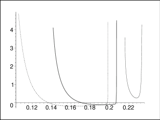
Figure 3: $(\partial^{2}E/\partial S^{2})_{J,Q}$ versus $m$ for $l=1$, $a=0.1$, $q=0$ (dotted), $0.1$ (thick-line), and $0.2$ (solid).

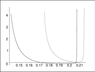
Figure 4: $(\partial^{2}E/\partial S^{2})_{J,Q}$ versus $m$ for $l=1$, $q=0.1$, $a=0.1$ (thick-line), and $0.15$ (solid).

Figure 5: $(\partial^{2}E/\partial S^{2})_{J,Q}$ versus $a$ for $l=1$, $m=0.2$, $q=0.2$ (thick-line), $0.15$ (dotted), and $0.1$ (solid).

Figure 6: $(\partial^{2}E/\partial S^{2})_{J,Q}$ versus $a$ for $l=1$, $q=0.1$, $m=0.15$ (dotted), and $0.2$ (solid).

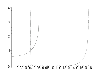
Figure 7: $(\partial^{2}E/\partial S^{2})_{J,Q}$ versus $q$ for $l=1$, $m=0.2$, $a=0.2$ (solid), and $0.1$ (dotted).

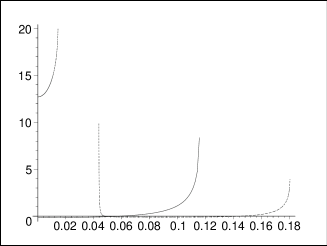
Figure 8: $(\partial^{2}E/\partial S^{2})_{J,Q}$ versus $q$ for $l=1$, $a=0.1$, $m=0.1$ (solid), $0.15$ (thick-line), and $0.2$ (dotted).

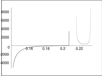
Figure 9: Determinant of Hessian matrix versus $m$ for $l=1$, $a=0.1$, $q=0.1$ (thick-line), and $0.2$ (dashed).

Figure 10: Determinant of Hessian matrix versus $q$ for $l=1$, $m=0.2$, $a=0.2$ (dotted), and $0.1$ (solid).

Figure 11: Determinant of Hessian matrix versus $q$ for $l=1$, $a=0.1$, $m=0.15$ (dashed), $0.2$ (thick-line), and $0.22$ (solid).

Figure 12: Determinant of Hessian matrix versus $a$ for $l=1$, $m=0.2$, $q=0.15$ (dotted), and $0.1$ (solid).

In the grand-canonical ensemble, the thermodynamic variables are the entropy, the charge and the angular momentum. The determinant of the Hessian matrix can be calculated numerically. Some typical results of these calculations are displayed in Figs. 9-12. As one can see from Fig. 9 which shows the $m$ dependence of the determinant of Hessian matrix, for a given value of $a$ and large values of $q$, the hole is stable, but for small values of $q$, only the extreme case is stable. The $q$ dependence of the determinant of the Hessian matrix are shown in Figs. 10 and 11. Figure 10 shows that for large values of $m$ and $a$ we encounter a single stable phase, while for large $m$ and small $a$ the only stable phase is the nearly extremal hole. We also find that for small $a$ the hole is stable for large $m$ and unstable for small $m$. For intermediate $m$ only the nearly extreme hole is stable (see Fig. 11). The $a$ dependence of the determinant of the Hessian matrix (Fig. 12) shows that for large values of $m$, when $q$ is large the only stable phase is the nearly extreme hole, but as $q$ decreases a stable low angular momentum phase will appear. The comparison of the figures of the canonical and grand-canonical ensemble shows that the region of stability is smaller in the latter case as stated before, and there are cases that even the extreme hole is not stable in the grand-canonical ensemble.

VI Closing Remarks

In this paper, we used the counterterm method to calculate the conserved quantities and the Euclidean action of the four-dimensional Kerr-Newman-dS black hole. Also we obtained a generalized Smarr formula for the mass as a function of the entropy, the angular momentum and the electric charge and showed that these quantities satisfy the first law of thermodynamics associated to the cosmological horizon. Since there is no well-defined thermodynamics for the asymptotically de Sitter black holes, a local investigation of the thermodynamics is necessary. Our investigation of the boundary-induced counterterm prescription (2) at finite distances has allowed us to obtain a number of interesting results, which we recapitulate here.

We were able to compute the quasilocal energy, the temperature, and the Hessian matrix of the energy with respect to $S$ and $Q$ for arbitrary values of the parameters of the Reissner-Nordstom-dS black hole analytically. We found that the temperature at fixed $r$ is the product of $\kappa_{H}/2\pi$ and the redshift factor. We perform a stability analysis both in the canonical and grand-canonical ensemble, and obtained a complete phase diagrams. We found that at a fixed value of $r$ there exists two stable phases separated by an unstable phase with intermediate mass value. That is, charge causes the low mass black hole to be stable, a fact which is not true for the Schwarzschild-dS black holes.

We also computed the determinant of the Hessian matrix, quasilocally, for arbitrary values of the parameters of the Kerr-Newman-dS₄ solution, apart from the mild reality restrictions considered in Sec. III. These quasilocal quantities are intrinsically calculable numerically at fixed $r$ without any reference to a background spacetime. By finding the parameters $a$, $m$ and $q$ in terms of the thermodynamic quantities $S$, $J$ and $Q$, we regarded the interior of the quasilocal surface as a thermodynamic system whose energy $E$ is a function of $S$, $J$ and $Q$. We studied the stability of the Kerr-Newman-dS black hole both in the canonical and grand-canonical ensembles. Thereby we encountered an interesting phase structure. We found that in the canonical ensemble the extreme black hole is stable for all the allowed values of the metric parameters while this is not true in the grand-canonical ensemble. The stability analysis in the canonical ensemble yielded results that are in qualitative agreement with previous investigations carried out by using the ADM mass parameter Davies . This stability analysis is, of course local, and phase transitions to other spacetimes of lower free energy might exist.

References

- (1) A. Strominger, J. High Energy Phys. 10, 034 (2001); 11, 049 (2001); V. Balasubramanian, P. Horova, and D. Minic, ibid. 05, 043 (2001); E. Witten, hep-th/0106109; D. Mu-In Park, Phys. Lett. B440, 275 (1998); S. Nojiri and S. D. Odintsov, ibid. 519, 145 (2001); J. High Energy Phys. 12, 033 (2001); Phys. Lett. B 523, 165 (2001); 528, 169 (2002); T. Shiromizu, D. Ida, and T. Torii, J. High Energy Phys. 11, 010 (2001); R. G. Cai, Phys. Lett. B 525, 331 (2002); Nucl. Phys. B628, 375 (2002); R. G. Cai, Y. S. Myung, and Y. Z. Zhang, Phys. Rev. D 65, 084019 (2002); R. Bousso, A. Maloney, and A. Strominger, ibid. 65, 104039 (2002); M. Spradlin and A. Volovich, ibid. 65, 104037 (2002); A. J. M. Medved, hep-th/0205251; V. Balasubramanian, J. D. Boer and D. Minic, hep-th/0207245; K. Skenderis, Class. Quantum Grav. 19, 5649 (2002).
- (2) R. G. Cai, Phys. Lett. B 525, 331 (2002); hep-th/0112253; M. Cvetic, S. Nojiri and S. D. Odintsov, Nucl. Phys. B628, 295 (2002).
- (3) T. Padmanabhan, Mod. Phys. Lett. A17, 923 (2002); Class. Quantum Grav. 19 5387 (2002).
- (4) M. H. Dehghani, Phys. Rev. D 65, 104030 (2002).
- (5) J. D. Beckenstein, Phys. Rev. D 7, 2333 (1973).
- (6) S. W. Hawking, Nature 248, 30 (1974) ; Comm. Math. Phys. 43, 199 (1975).
- (7) S. W. Hawking and C. J. Hunter, Phys. Rev. D 59, 044025 (1999); C. J. Hunter, ibid. 59, 024009 (1999); S. W. Hawking, C. J. Hunter and D. N. Page, ibid. 59, 044033 (1999).
- (8) R. B. Mann, Phys. Rev. D 60, 104047 (1999); ibid 61, 084013 (2000).
- (9) G. W. Gibbons and S. W. Hawking, Phys. Rev. D 15, 2738 (1977).
- (10) G. W. Gibbons and S. W. Hawking, Commun. Math Phys. 66, 291 (1979).
- (11) J. D. Brown and J. W. York, Phys. Rev. D 47, 1407 (1993).
- (12) K. C. K. Chan, J. D. E. Creighton and R. B. Mann, Phys. Rev. D 54, 3892 (1996).
- (13) E. A. Martinez, Phys. Rev. D 50, 4920 (1994).
- (14) M. Hennigson and K. Skenderis, J. High Energy Phys. 7, 023 (1998).
- (15) V. Balasubramanian and P. Kraus, Commun. Math. Phys. 208, 413 (1999).
- (16) R. Emparan, C.V. Johnson and R. C. Myers, Phys. Rev. D 60, 104001 (1999).
- (17) V. Balasubramanian, J. deBoer and D. Minic, Phys. Rev. D 65, 123508 (2002); Klemm, Nucl. Phys. B625, 295 (2002).
- (18) A. M. Ghezelbash and R. B. Mann, J. High Energy Phys. 01, 005 (2002).
- (19) M. H. Dehghani, Phys. Rev. D 65, 104003 (2002).
- (20) P. Kraus, F. Larsen and R. Siebelink, Nucl. Phys. B563, 259 (1999).
- (21) S. Das and R. B. Mann, J. High Energy Phys. 08, 033 (2000); D. Birmingham and S. Mokhtari, Phys. Lett. B508, 365 (2001).
- (22) M. H. Dehghani, Phys. Rev. D 65, 124002 (2002).
- (23) M. H. Dehghani, Phys. Rev. D 66, 044006 (2002).
- (24) M. H. Dehghani and R. B. Mann, Phys. Rev. D 64, 044003 (2001).
- (25) S. de Haro, K. Skenderis and S. N. Solodukhin, Commun. Math. Phys. 217, 595 (2001); M. Bianchi, D. Z. Freedman and K. Skenderis, Nucl. Phys. B631, 159 (2002); M. Taylor-Robinson, hep-th/0002125.
- (26) M. M. Caldarelli, G. Cognola, and D. Klemm, Class. Quantum Grav. 17, 339 (2000).
- (27) R. C. Tolman, Phys. Rev. 35, 904 (1930).
- (28) J. D. Brown, J. Creighton and R. B. Mann, Phys. Rev. D 50, 6394 (1994).
- (29) C. Peca and J. P. S. Lemos, Phys. Rev. D 59, 124007 (1999).
- (30) M. Cvetic and S. S. Gubser, J. High Energy Phys. 04, 024 (1999).
- (31) S. S. Gubser and I. Mitra J. High Energy Phys. 08, 018 (2001).
- (32) P. C. Davies, Class. Quantum Grav. 6, 1909 (1989).