UNIVERSITÉ LIBRE DE BRUXELLES
Faculté des Sciences
Service de Physique Théorique et Mathématique

Issues in electric-magnetic duality

Dissertation présentée en vue de l’obtention

du grade de Docteur en Sciences

Xavier Bekaert

Année académique 2001–2002

Remerciements

Avant toute chose, je constate qu’il est difficile de rendre justice aux innombrables personnes qui ont pu m’aider et m’influencer durant ces quatre ans de thèse.

Il va sans dire que les travaux présentés ici n’ont pas été accomplis de manière isolée. Ils trouvent tous leurs sources dans diverses discussions et dans de nombreuses collaborations. Je voudrais commencer par remercier toutes les personnes avec qui j’ai eu la joie de travailler directement. Ma thèse a débuté par une collaboration avec Christiane Schomblond et Bernard Knaepen. À l’instar de nombreuses discussions avec Glenn Barnich, cette collaboration m’a familiarisée avec les techniques de la cohomologie BRST, ce qui m’a été extrêmement utile par la suite. Elle a été suivie par une collaboration avec Marc Henneaux et Alexander Sevrin sur les déformations des théories de champs de jauges chiraux. J’ai eu ensuite le plaisir de travailler avec Odile Saliu et Constantin Bizdadea en Roumanie sur un projet que nous n’avons malheureusement pas réussi à conclure. Cependant j’ai tiré grand bénéfice de cette rencontre puisqu’elle m’a amené à apprendre concrètement la quantification BRST Hamiltonienne. La rencontre avec Sorin Cucu et les travaux qui en suivirent ont été une longue expérience très enrichissante. Les visites d’Andres Gomberoff à Bruxelles m’ont donné l’opportunité de travailler sur la non-conservation de la charge électrique en supergravité. Dernièrement, j’ai effectué une brève incursion dans la phénoménologie des branes avec Nicolas Boulanger et Justin Vazquez-Poritz. Cet doctorat s’achève par une collaboration avec Nicolas Boulanger et Marc Henneaux sur la dualisation de la gravitation linéarisée.

Parmi les personnes avec qui j’ai conversé pendant la durée de cette thèse, je remercie particulièment toutes celles qui ont participé aux divers groupes d’études et séminaires informels qui ont jalonné ces quatres années. J’ai particulièrement apprécié les multiples échanges que nous avons pu avoir entre membres du service de physique théorique et du groupe de physique mathématique des interactions fondamentales de l’ULB. J’ai également profité des rencontres, plus rares mais tout aussi enrichissantes, avec les membres du Centro de Estudios Científicos de Chile.

J’ai partagé un bureau avec Nicolas Boulanger pendant trois ans. Ce dernier a pu faire connaissance avec mes humeurs changeantes et je le félicite pour sa patience. Cette cohabitation prolongée m’a beaucoup apporté sur les plans de la physique et de l’amitié.

C’est avec plaisir que je remercie également la chaleureuse hospitalité roumaine dont je n’ai jamais rencontré dans nul autre pays d’analogue aussi frappant. En particulier, un grand merci à tous les amis roumains de l’Université de Craiova.

Je suis très reconnaissant à Glenn Barnich, Bernard Knaepen, et Olivier Debliquy pour leur aide répétée et patiente en informatique. Cette thèse n’aurait probablement jamais pu voir le jour sans les milles coups de main qu’ils m’ont donnés dans ce domaine qui conservera toujours pour moi sa part d’absurde.

Je suis également très reconnaissant à Fabienne Deneyn pour son aide indispensable dans bon nombre de questions administratives.

Je remercie chaleureusement Christiane Schomblond pour sa disponibilité, son aide scientifique et son soutien moral durant ces années d’études.

Je remercie vivement mon promoteur Marc Henneaux pour ses idées stimulantes, ses remarques, ses encouragements et ses conseils opportuns lors de tous les moments décisifs du long parcours scientifique (et initiatique) qu’est le doctorat.

Une fois de plus, je remercie Christiane Schomblond, Marc Henneaux et Nicolas Boulanger; cette fois ci, pour leur lecture attentive de cette thèse et leurs commentaires constructifs. Pour ces mêmes raisons, je remercie également les membres du jury Laurent Houart, Alexander Sevrin, Mario Tonin et Michel Tytgat.

Je n’ai pas tant d’amis que pour ne pouvoir les citer tous ici mais, de peur d’en omettre un seul, je préfère les remercier tous ensemble, d’un seul élan. Chacun d’entre eux s’y reconnaitra aisément car ils savent combien leur amitié m’est chaque jour indispensable.

Pour terminer, mes remerciements vont à mes parents pour toutes ces innombrables choses, petites ou grandes, sans lesquelles ce travail n’aurait certainement pas pu voir le jour.

Chapter 1 Introduction to electric-magnetic duality

Electric-magnetic duality symmetry has a rather old history, going back to the birth of Maxwell’s equations:

$${\bf\nabla}\cdot{\bf E} = \rho\,,$$ (1.0.1)

$${\bf\nabla}\cdot{\bf B} = 0\,,$$ (1.0.2)

$${\bf\nabla}\times{\bf B} = {\bf j}\,+\,\frac{\partial{\bf E}}{\partial t}\,,$$ (1.0.3)

$${\bf\nabla}\times{\bf E} = -\,\frac{\partial{\bf B}}{\partial t}\;\;.$$ (1.0.4)

It seems likely that the symmetric role played by the electric and the magnetic fields in the laws of electromagnetism, has been one of the motivations of Maxwell to introduce in the Ampère law, the “displacement current” $\frac{\partial{\bf E}}{\partial t}$, which was not sanctioned by experiment at that time. Significantly, this led him to the correct equation (1.0.3). When there is no electric current (${\bf j}=0$) this equation takes indeed the same form as the Faraday law (1.0.4) up to a change of sign. Maxwell was known to have an aesthetic appreciation for mathematical structures: “I always regarded mathematics as the method of obtaining the best shapes and dimensions of things; and this meant not only the most useful and economical, but chiefly the most harmonious and the most beautiful”. In this light, it is reasonable to accept the conclusion of Roger Penrose: “It would seem that the symmetry of these equations and the aesthetic appeal that this symmetry generated must have played an important role for Maxwell in his completion of these equations” [2].

1.1 Modifying Maxwell’s equations with Dirac

The above-mentioned symmetry can be more precisely expressed as the invariance of sourceless ($\rho={\bf j}=0$) Maxwell’s equations under a “rotation” of the electric and magnetic fields

$${\bf E} \rightarrow \,\,\cos\alpha\,{\bf E}-\sin\alpha\,{\bf B},$$

$${\bf B} \rightarrow +\sin\alpha\,{\bf E}+\cos\alpha\,{\bf B}.$$ (1.1.1)

A physical important point is that the energy-momentum tensor is also left invariant under the transformation (1.1.1). This can be easily checked for the energy and momentum densities of the electromagnetic field:

$${\cal E}=\frac{1}{2}\,({\bf E}^{2}+{\bf B}^{2}),\quad{\bf{\cal P}}={\bf E\times B}\,,$$ (1.1.2)

as well as for the stress tensor $T_{ij}=-E_{i}\,E_{j}-B_{i}\,B_{j}+{\cal E}\,\delta_{ij}$.

1.1.1 Magnetic monopoles

Basically, the equation (1.0.2) states that if one breaks a magnet bar in two pieces in its middle, one always obtains two smaller magnets and never a North pole in one hand and a South pole in the other hand, as it could occur for an electric dipole. The absence of isolated magnetic charge in Maxwell’s equations (1.0.1)-(1.0.4) spoils the possibility of the symmetry (1.1.1) in the presence of sources. Since it appears deceiving that Nature is deprived from such a beautiful symmetry, it would be satisfactory to find an explanation of its absence. The first natural step is to assume the existence of magnetic pole and investigate whether this leads to any contradiction with known principles. This is what Dirac did in 1931 [3].

To establish the symmetry between the electric and magnetic fields in the presence of sources, we have to assume the existence of magnetic densities of charge and current $\rho_{m}$ and ${\bf j}_{m}$, in addition to the usual electric charge density and current $\rho_{e}=\rho$ and $j_{e}={\bf j}$. The Maxwell equations then take the form

$$\mathbf{\nabla}\cdot\bf{E} = \rho_{e}\,,$$

$$-\bf{\nabla}\times\bf{E} = \bf{j}_{m}+\frac{\partial\bf{B}}{\partial t}\,,$$

$$\bf{\nabla}\cdot\bf{B} = \rho_{m}\,,$$

$$\bf{\nabla}\times\bf{B} = \bf{j}_{e}+\frac{\partial\bf{E}}{\partial t}\,.$$ (1.1.3)

The EM symmetry can easily be seen by rewriting the modified Maxwell equations as

$$\bf{\nabla}\cdot(\bf{E}+i\,\bf{B}) = \rho_{e}+i\,\rho_{m}\,,$$

$$\bf{\nabla}\times(\bf{E}+i\,\bf{B}) = i\,\left[\left(\bf{j}_{e}+i\,\bf{j}_{m}\right)+\frac{\partial}{\partial t}\left(\bf{E}+i\,\bf{B}\right)\right]\,.$$ (1.1.4)

In terms of the fields, the rotation (1.1.1) reads :

$$\bf{E}+i\,\bf{B} \rightarrow e^{i\,\alpha}\left(\bf{E}+i\,\bf{B}\right)\,,$$

$$\rho_{e}+i\,\rho_{m} \rightarrow e^{i\,\alpha}\left(\rho_{e}+i\,\rho_{m}\right)\,,$$

$$\bf{j}_{e}+i\,\bf{j}_{m} \rightarrow e^{i\,\alpha}\left(\bf{j}_{e}+i\,\bf{j}_{m}\right)\,.$$ (1.1.5)

The electromagnetic energy density reads

$${\cal E}=\frac{1}{2}\,|\bf{E}+i\,\bf{B}|^{2}\,,$$ (1.1.6)

which is manifestly invariant under (1.1.5).

As noticed in [4], it is a matter of convention to speak of a single electrically charged but not magnetically charged particle : “The only meaningful question is whether or not all particles have the same ratio of magnetic to electric charge.” If they do, we can choose an appropriate duality rotation which makes the magnetic charge and current to vanish, and we recover the ordinary Maxwell equations.

1.1.2 Charge quantization

In 1931 Dirac showed that if one wants the associated quantum theory to be consistent in the presence of an electric charge $e$ and a magnetic monopole of charge $g$, they have to satisfy the following quantization relation [3]

$$e\,g=n\,h\quad\quad n\in\mathbb{N}\,.$$ (1.1.7)

Therefore the existence of a single magnetic charge could explain the quantization of electric charge in Nature. This is how Dirac left the subject in 1931. He came back to it in 1948, to clarify their dynamical behaviour [5]. However many questions were left unresolved, including the puzzling remark that the quantization condition (1.1.7) does not respect the proposed rotational symmetry (1.1.1). Several of these questions will be addressed in the sequel; the chapter 6 is devoted to the particular topic of the charge quantization condition.

The known unit of pure electric charge is known to be small: $e^{2}/4\pi=\alpha\ll 1$. We point out that (1.1.7) implies that the magnetic charge of a monopole is expected to be large in natural units: $g\gg 1$ since $e\ll 1$.

The 1931 and 1948 Dirac’s arguments for charge quantization were essentially topological in nature. It seems to be the first notable appearance of topology in twentieth century physics. It is surprising that one had to wait until the 1959 paper of Aharonov and Bohm (almost thirty years after Dirac’s monopole !) to pinpoint a significant instance of an interaction between topology and physics. As is well known, it has been followed by an amazing number of other fruitful appearances in many areas of theoretical physics during the past four decades.

1.1.3 Dirac’s aesthetic

In some sense, Dirac pursued Maxwell’s quest of mathematical beauty by modifying the electromagnetism equations on aesthetic grounds. Dirac might be the physicist who insisted the most on the role played by the inherent mathematical beauty of physics equations. At the advanced age of 78, he described his main attitude regarding mathematics and physics: “A good deal of my research work in physics has consisted in not setting out to solve some particular problem, but simply examining mathematical quantities of a kind that physicists used and trying to fit them together in an interesting way, regardless of any application that the work may have. It is simply a search for pretty mathematics. It may turn out later that the work does have an application. Then one has good luck.” [7].

Nevertheless, since the existence of the magnetic monopole is still not experimentally established, it is not yet clear if Dirac’s monopole will follow the same fate as Maxwell’s displacement current or Dirac’s positron. Anyway, the investigation of the magnetic monopole is, according to David I. Olive, “perhaps the single contribution that best illustrates Dirac’s fearlessness” because “it certainly required courage to initiate a theory of an undetected particle. Because of what Dirac found, that theory has continued to intrigue researchers and continues to develop (…) The story of magnetic monopole is still far from complete and indeed promises more revelations”. The role played by dualities in the emergence of the M-theory conjecture and the better understanding of EM duality obtained in this framework extensively confirms the fertility of Dirac’s seminal idea as well as Dirac’s “good luck” in discovering new areas in physics.

1.2 Preliminary remarks

Let us stress an important restriction in the present thesis: the absence of fermions. Despite the fact that supersymmetry and, more recently, supergravity together with superstring theory gave birth to numerous developments in the subject, we will restrict ourselves to purely bosonic theories (or to the bosonic sectors of supersymmetric ones). This is legitimated by the fact that fermions are inert under EM duality rotation in all known cases, therefore they will play no role in the topics discussed here.

In order to separate the original results obtained during this thesis from the works on which they are based, we reserve the label “theorem” to the main original mathematical material presented here. Results imported from outside will be referred to as lemmas or propositions, without respect of their scientific importance. Multiple citations are given in the chronological order of publication. Mathematical definitions are written in bold type. Physical definitions are italicized.

We use a unit system for which $\hbar=c=1$.

1.3 Overview of the thesis

In the chapter 2, our discussion will mainly focus on the non-manifest classical duality symmetry of the equations of motion (derived from standard actions) of various kind of bosonic brane electrodynamics. Our theorem 1 is given and its relevance for four-dimensional non-linear electrodynamics is explained [10]. A new discussion of open brane charge in the language of relative (co)homology is presented in section 2.7.

Possible generalizations of EM duality for linearized gravity are discussed in the chapter 3. We make some comments on the differences with electrodynamics. The main result of this chapter is our theorem 2 which generalizes the Poincaré lemma to tensors in arbitrary representations of the general linear group $GL(D,\mathbb{R})$ [11]. This theorem allows a systematic discussion of duality properties of such tensors that is done in section 3.9.

The chapter 4 is devoted to manifest duality symmetry. Different ways to implement the duality symmetry at the level of the action are reviewed. In the section 4.4, we introduce a topological derivation of the D-brane-boundary rule from the Wess-Zumino coupling in the duality-symmetric formulation of IIA supergravity.

We perform the Batalin-Vilkovisky quantization of Maxwell’s theory in its manifestly Lorentz and duality symmetric formulation in the chapter 5 [12]. The Hamiltonian BRST quantization of Maxwell’s theory is reviewed.

In the chapter 6, we first review some quantization conditions that generalizes Dirac’s work and then we derive a quantization condition of the Chern-Simons coefficient of eleven-dimensional supergravity in section 6.3 [13].

The chapter 7 is a discussion on consistent deformations of self-dual gauge fields in the M-theory perspective. Our no-go theorem 3 on local consistent deformations is presented [14, 15, 10]. More specifically, in the section 7.4 we also compute all consistent, continuous, local and Lorentz invariant deformations of a system of Abelian self-dual vector gauge fields [10]. Our no-go theorem 4 on deformations of a mixed symmetry type gauge field of interest in gravity duality properties is also given [16].

The first four appendices A-D review mathematical definitions (that the reader might be familiar with) which are used throughout the thesis in order to be as much self-contained as possible (and to provide some reference map for the author himself not to get completely lost in this mathematical jungle !). Some choices of conventions and notations are also presented there. All this material is placed at the end of the thesis to separate the physical exposure from the necessary mathematical machinery exposition.

The full proofs of the three theorems 1-3 are given in the last three appendices E-G since they are technical and lengthy.

Chapter 2 Classical duality in bosonic brane electrodynamics

This introductory chapter is aimed to give an overview (far from being complete) of Maxwell’s electrodynamics generalizations which appear in string/M-theory, and of several possible extensions of the electric-magnetic (EM) duality symmetry (1.1.1) in this context.

In the first section we generalize the concept of EM duality to higher dimensional sources and spacetime. The electrokinematics section 2.2 tries to motivate geometrically the use of $p$-form gauge fields in generalizing Maxwell’s theory. It may be skipped by the reader without inconvenience. The section 2.3 introduces the mathematical tools chosen to deal with extended sources. In section 2.4, linear electrodynamics for extended objects is presented and its properties are discussed in details. The section 2.5 gives up the linearity assumption and generalizes the duality transformation in the (Abelian) self-interacting context. In the short section 2.6, we briefly discuss some consequences of the addition of a theta term in the Lagrangian in dimensions multiple of $4$. A reformulation of charge non-conservation issues in the presence of a Chern-Simons (CS) coupling is presented in the language of de Rham currents in section 2.7. We end up this chapter by applying the previous discussion to two specific electrodynamics with CS coupling in the last section 2.8.

2.1 Let’s use differential forms

In order to render higher dimensional generalizations more transparent in the next section, we will reformulate the modified Maxwell equations in terms of differential forms. Their use is very convenient because their minimal coupling with a background metric is automatically implemented. To proceed, we define the electric and magnetic fields as components of the field strength two-form $F$: the electric and magnetic fields are the components of the field strength: $E^{i}\equiv F^{0i}$, $B^{i}\equiv-(*F)^{0i}=\frac{1}{2}\epsilon^{ijk}F_{jk}$. The charge and current densities are, respectively, the time and spatial components of a one-form $J$. Equations (1.1.3) are rewritten as

$$d\left(\begin{array}[]{c}F\\ F\end{array}\right)=\left(\begin{array}[]{c}*J_{m}\\ J_{e}\end{array}\right)\,.$$ (2.1.1)

In the absence of magnetic monopole (i.e. $J_{m}=0$), the Poincaré lemma is used to derive from the Bianchi identity ($dF=0$) the existence of a potential vector $A$ such that $F=dA$. The field equation $d*F=*J_{e}$ arises from the Maxwell action

$$S_{M}[A,J_{e}]=-\frac{1}{2}\int F\wedge*F+\int A\wedge*J_{e}.$$ (2.1.2)

When $J_{m}\neq 0$, one introduces a Dirac string $G$ such that $d*G=*J_{m}$; therefore the modified Bianchi $dF=*J_{m}$ gives $F=dA+*G$. The field equation is derived from the same action with $F$ replaced by $dA+*G$. In subsection 2.3 we will explain in more details the precise definition of the Dirac strings and their use to deal with magnetic monopoles in an action principle. Electric charges and magnetic monopoles are not the only possibilities. Particles carrying both electric and magnetic charges also make sense, they have been christened as dyons by Schwinger [17].

2.1.1 Duality rotation

The duality rotation (1.1.5) takes the form

$$\left(\begin{array}[]{c}F\\ $*$F\end{array}\right)\rightarrow R\left(\begin{array}[]{c}F\\ $*$F\end{array}\right)\,,$$ (2.1.7)

$$\left(\begin{array}[]{c}J_{m}\\ J_{e}\end{array}\right)\rightarrow R\left(\begin{array}[]{c}J_{m}\\ J_{e}\end{array}\right)\,,$$ (2.1.12)

where $R\in SO(2)$.

Let us stress two points that arise if the fieldstrength is expressed in terms of a gauge field $A$ (which is the fundamental field in the variational principle). The first point is that the duality rotation is only well-defined on-shell. In the chapter 4.1, a formulation for which duality rotation is an off-shell symmetry is presented. For an infinitesimal rotation of angle $\delta\alpha$ one has $\delta F=*F\,\delta\alpha$, therefore the variation of the Bianchi identity requires $d*F=0$ because $d\,\delta F=\delta\,dF=0$. The second point is that the duality rotation becomes a non-local map when expressed in terms of the gauge field $A$. Indeed, for an infinitesimal rotation of angle $\delta\alpha$ we have $\delta A=d^{-1}(*F)\,\delta\alpha$, where $d^{-1}$ stands for the non-local operator which is the inverse of the differential $d$.

2.1.2 Energy-momentum tensor

Let $S=\int{\cal L}(g_{\mu\nu})$ be a matter action in a metric background $g_{\mu\nu}$. The energy-momentum tensor is defined as

$$T_{\mu\nu}*1=-2\,\frac{\partial\,{\cal L}}{\partial g^{\mu\nu}},$$ (2.1.13)

where $*1$ is the volume form on $\cal M$. The Maxwell energy-momentum tensor is defined by using the differential form ${\cal L}_{Maxwell}=-\frac{1}{2}\,*F\wedge F$ in (2.1.13) to get

$$T^{Maxwell}_{\mu\nu}*1=F_{\mu}\,F_{\nu}\,+\,g_{\mu\nu}\,{\cal L}_{Maxwell}\,,$$ (2.1.14)

where $F_{\mu}$ is a one-form defined by (B.6.12). We made use of the identity (B.6.11).

Let us introduce the $(D-3)$-form $(*F)_{\mu}$ defined by (B.6.12). The relation

$$*(*F)_{\mu}\wedge(*F)_{\nu}-*F_{\mu}\wedge F_{\nu}=2g_{\mu\nu}\,{\cal L}_{Maxwell}\,,$$ (2.1.15)

follows from the identity (B.6.13). So, one can rewrite the energy-momentum tensor in a more convenient form [18]

$$2\,T^{Maxwell}_{\mu\nu}*1=*F_{\mu}\wedge F_{\nu}\,+\,*(*F)_{\mu}\wedge(*F)_{\nu}\,.$$ (2.1.16)

It is now straightforward to check the invariance of the energy-momentum $T_{\mu\nu}$ since $*^{2}F=-F$.

2.2 Brane electrokinematics

Having string theory in mind, it is natural to try to extend the usual Maxwell point particles electrodynamics to incorporate extended objects. The objects we will consider are the so-called $p$-branes. They are ($p+1$)-dimensional submanifolds of the $D$-dimensional spacetime manifold $\cal M$ (called the target space in this context) with the induced metric of signature $(-,+,\ldots,+)$. One has $0\leq p+1\leq D$.

The limiting case $p=-1$ corresponds to instantons which are localized both in space and time. The $0$-branes are the standard relativistic particles while the $1$-branes are called strings and the $2$-branes have been christened membranes. This is summarized in the table 2.1

$p$	$p$-brane	worldhistory
$-1$	instanton	point
$0$	particle	worldline
$1$	string	worldsheet
$2$	membrane	worldvolume
$3$	$3$-brane	worldvolume
$\vdots$	$\vdots$	$\vdots$

Table 2.1: $p$-brane dictionary

In 1986, Teitelboim and Nepomechie already studied generalized electrodynamics and the Dirac quantization condition in the presence of magnetic extended sources [19, 20].

A $p$-brane worldvolume is a manifold $\in\Lambda_{p+1}({\cal M})$ (= the space of all $(p+1)$-dimensional smooth orientable submanifolds in the manifold ${\cal M}$) defined by the parametric equations $x^{\mu}=x^{\mu}(\tau,\sigma^{1},\dots,\sigma^{p})$. We assume the target space and the worldvolume to be smooth orientable manifolds throughout this thesis. The index $\mu$ is the spacetime index ($\mu=0,\dots,D-1$), $\tau$ is the time coordinate along the brane worldvolume and $\sigma=(\sigma^{1},\dots,\sigma^{p})$ denote the set of spatial coordinates.

The remaining of this section tries to motivate and to discuss on geometrical grounds the introduction of $(p+1)$-form gauge fields when considering $p$-branes. It is heuristic in spirit and is not essential for understanding the following “brane electrodynamics”.

2.2.1 Gauge field theory of branes

In a naive gauge field theory of branes à la Schrödinger, we would consider “wave-functionals” $\Psi[x(\sigma)]$ defined on the configuration space $\Lambda_{p}({\cal M})$.

We define a $p$-derivative $\frac{\delta}{\delta x^{\mu}(\sigma)}$ which generalizes the usual derivative $\frac{\partial}{\partial x^{\mu}}$ and the loop-derivative $\frac{\delta}{\delta x^{\mu}(s)}$ [21]. It can be seen (without genuine mathematical rigor) in the following way: Given $x^{\nu}(\sigma^{\prime})$, we can make a $\delta$-function variation in the direction $\mu$ at any point of coordinates $\sigma$. This variation gives $x^{{}^{\prime}\nu}(\sigma^{\prime})=x^{\nu}(\sigma^{\prime})+\Delta\delta^{\nu}_{\mu}\delta(\sigma^{\prime}-\sigma)$. The derivative $\frac{\delta}{\delta x^{\mu}(\sigma)}$ of the functional $\Psi[x]$, defined on $\Lambda_{p}({\cal M})$, is defined by

$$\frac{\delta\Psi[x]}{\delta x^{\mu}(\sigma)}=\lim_{\Delta\rightarrow 0}\frac{\Psi[x^{\prime}]-\Psi[x]}{\Delta}.$$ (2.2.1)

The set of all $p$-derivatives $\{\frac{\delta}{\delta x^{\mu}(\sigma)}\}$ provides a basis of the tangent space to $\Lambda_{p}({\cal M})$.

Formally, we can now write a Dirac equation for a “wave-functional” $\Psi[x(\sigma)]$ (invariant under Lorentz transformation of the embedding Minkowski space) by extending naturally the usual Dirac equation. Let us assume that this “first quantized” theory possess a global invariance under an internal Lie group $G$ (which, for generality, will be assumed to be semi-simple) acting as

$$\Psi[x(\sigma)]\rightarrow\exp(ig\alpha)\,\Psi[x(\sigma)]$$ (2.2.2)

where $\alpha$ is an element of the matrix representation of the Lie algebra ${\cal G}$ tangent to the group $G$. We would extend (2.2.2) into a local gauge invariance, i.e. replace $\alpha$ by a $x(\sigma)$-dependent matrix $\alpha[x(\sigma)]$ in (2.2.2). In order to preserve the invariance of the “Dirac equation”, we would replace the derivatives $\frac{\delta}{\delta x^{\mu}(\sigma)}$ by covariant derivatives $\frac{\Delta}{\Delta x^{\mu}(\sigma)}$.

To do so, let us introduce a ${\cal G}$-Lie-algebra-valued connection 1-form $A[x(\sigma)]$ defined on $\Lambda_{p}(M)$. The parallel transport of the “wave-function” along a path $x_{u}^{\mu}(\sigma)$ in $\Lambda_{p+1}(M)$, enters the theory through the equation

$$\delta_{\parallel}\Psi[x_{u}(\sigma)]=igA[x_{u}(\sigma)]\Psi[x_{u}(\sigma)]du,$$ (2.2.3)

where $g$ is a coupling constant. This equation defines the infinitesimal parallel transport of the wave-function from $x_{u}(\sigma)$ to $x_{u+du}(\sigma)$ as

$$\Psi_{\parallel}[x_{u+du}(\sigma)]=\Psi[x_{u+du}(\sigma)]+\delta_{\parallel}\Psi[x_{u}(\sigma)].$$ (2.2.4)

Hence, the covariant derivative of the wave-function is given by

$$\frac{\Delta}{\Delta x^{\mu}(\sigma)}\Psi[x_{u}(\sigma)]=\left(\frac{\delta}{\delta x^{\mu}(\sigma)}+igA[x_{u}(\sigma]\right)\Psi[x_{u}(\sigma)]$$ (2.2.5)

The searched-for covariantized “Dirac equation” will be invariant under the gauge transformation of the wave-function

$$\Psi[x(\sigma)]\rightarrow U[x(\sigma)]\Psi[x(\sigma)],$$ (2.2.6)

where $U[x(\sigma)]=\exp(ig\alpha[x(\sigma)])$ if, at the same time, $A$ transforms as a connection

$$A[x(\sigma)]\rightarrow\left(\frac{i}{g}\,\delta U[x(\sigma)]+U[x(\sigma)]A[x(\sigma)]\right)U^{-1}[x(\sigma)],$$ (2.2.7)

where $\delta$ is the exterior differential on $\Lambda_{p}({\cal M})$. As usual, this is the patching condition of the $A$ seen as a local connection on the principal bundle $P(\Lambda_{p}({\cal M}),G)$ of basis $\Lambda_{p}({\cal M})$ and of structure group $G$.

We can now parallel-transport the wave-function from $x_{0}(\sigma)$ to $x_{1}(\sigma)$ along the $p+1$-dimensional path $\Gamma_{p+1}$. The solution of (2.2.3) is then

$$\Psi[x_{1}(\sigma)]=P_{u}\exp\left[ig\int_{\Gamma_{p+1}}A\right]\Psi[x_{0}(\sigma)].$$ (2.2.8)

The symbol $P_{u}$ denotes path ordering in the $u$-parameter.

Up to now, we have no guarantee that the previous objects are well-defined and that nothing prevents the existence of the connection $A$. To address more rigorously this issue, we add a requirement necessary to make contact with standard local field theory: the requirement of locality. As shown in [22, 23] this will impose strong restrictions on the gauge group for $p\geq 1$.

2.2.2 Antisymmetric tensor fields as Abelian connections

The locality requirement states that along the path $\Gamma_{p+1}$, the connection $A$ should be given by [23]

$$A[x_{u}(\sigma)]\,du=\frac{1}{(p+1)!}\int_{\Gamma^{u}_{p}}A_{\mu_{1}\dots\mu_{p+1}}(x_{u})\,dx_{u}^{\mu_{1}}\wedge\dots\wedge dx_{u}^{\mu_{p+1}}$$ (2.2.9)

where $A_{\mu_{1}\dots\mu_{p+1}}$ are the components of a $(p+1)$-form on the spacetime manifold $\cal M$, and the integral is extended over the $p$-dimensional manifold $\Gamma^{u}_{p}\equiv x=x_{u}(\sigma)$ ($u$ is fixed). The exterior product $dx^{\mu_{1}}\wedge\dots\wedge dx^{\mu_{p+1}}$ is the tangent to the path $\Gamma_{p+1}$, and is equal to

$$dx^{\mu_{1}}\wedge\dots\wedge dx^{\mu_{p+1}}=\frac{\partial x^{[\mu_{1}}}{\partial\sigma^{1}}\dots\frac{\partial x^{\mu_{p}}}{\partial\sigma^{p}}\frac{\partial x^{\mu_{p+1}]}}{\partial u}d\sigma^{1}\wedge\dots\wedge d\sigma^{p}\wedge du.$$ (2.2.10)

An important constraint is that: in order to be well-defined, the parallel transport operator in (2.2.8) must be reparametrisation invariant, that is, it must remain invariant under general coordinate transformations of the coordinates $(u,\sigma^{1},\dots,\sigma^{p})\equiv(\xi^{0},\dots,\xi^{p})$ on $\Gamma_{p+1}$. Teitelboim proved by geometrical arguments that this is impossible for $p\geq 1$, except if the gauge group is Abelian [22]. In the Abelian case, the path ordering on $u$ is no longer necessary and the “integral” in the exponential of the parallel transport in (2.2.8) becomes the usual volume integral $\int_{\Gamma_{p+1}}A_{\mu_{1}\dots\mu_{p+1}}(x)\,dx^{\mu_{1}}\wedge\dots\wedge dx^{\mu_{p+1}}$, the reparametrisation invariance of which is well known.

In other words, Abelian $(p+1)$-forms do not allow for simple local non-Abelian extensions when $p\geq 1$. The possibility for $p=0$ is obvious, because it is nothing else than the Yang-Mills theory. It can even be proved that, under certain assumptions, the Yang-Mills theory is the unique local consistent non-trivial deformation of the free Abelian theory [24]. In the papers [25, 26, 27, 28], general local and continuous deformations of free Abelian forms of rank higher than one have been classified at first order in the coupling constant, using the powerful algebraic tools of homology (reviewed in chapter 7), thereby dropping any geometric prejudice. Though both already known and novel deformations were discovered, none of them had the required property that the gauge algebra becomes “genuinely” non-Abelian (i.e. at first order in the coupling constant $g$, as in the Yang-Mills construction). The possibility of non-local (or non-perturbative) extensions of antisymmetric tensor gauge fields of course remains, but such a theory (if it exists) is still lacking. Furthermore, it is not granted that such a theory could be really interpreted as a field theory of a connection for extended objects, as in the Abelian case explained here. Anyway, M-theory seems to require a non-Abelian extension of chiral $2$-forms (see chapter 7), hence there still exists some clues of the existence of a field theory (maybe “exotic”) of non-Abelian $(p+1)$-forms.

To conclude this subsection, let us briefly remark that a more precise mathematical formulation of antisymmetric tensors as connections for extended objects is provided by Abelian gerbes [30]. The Abelian $p$-gerbes are the generalization of bundles for $(p+2)$-field strength. For $p=0$, they correspond to the usual principal bundle formulation of point particle gauge theory. Recently, a global approach to the study of duality transformations has been undertaken in the geometrical setting of gerbes [31].

2.3 de Rham currents and Dirac branes

We start by introducing a convenient tool to deal with charged extended objects: the de Rham currents.

2.3.1 Extended sources as de Rham currents

Let ${\cal W}_{p+1}$ be the worldvolume of a $p$-brane with charge density $q$. The image of ${\cal W}_{p+1}$ by the Poincaré dual map (C.2.2) is the differential form $P({\cal W}_{p+1})=*\alpha_{p+1}$ of form degree $D-p-1$. Its current $J_{p}$ is defined to be equal to $q\alpha_{p+1}$. Explicitly, one has

$$J^{\mu_{1}\ldots\mu_{p+1}}(x)=q\int_{{\cal W}_{p+1}}\,\delta^{(D)}\left(x-W(\xi)\right)dW^{\mu_{1}}\wedge\ldots\wedge dW^{\mu_{p+1}}\,,$$ (2.3.1)

if $x^{\mu}=W^{\mu}(\xi)$ is the parametric equation of the $p$-brane worldvolume ${\cal W}_{p+1}$.

For several, say $n$, branes of worldvolumes ${\cal W}^{(i)}_{p+1}$ and charge $q_{i}$ ($i=1,\ldots,n$), we define the manifold ${\cal W}_{p+1}$ to be the sum ${\cal W}_{p+1}\equiv\sum_{i}{\cal W}^{(i)}_{p+1}$ (which is well defined in $\Omega_{*}({\cal M};\mathbb{Z})$). Without loss of generality the submanifolds ${\cal W}^{(i)}_{p+1}$ are assumed not to intersect with each other, ${\cal W}^{(i)}_{p+1}\cap{\cal W}^{(j)}_{p+1}=\emptyset$ for $i\neq j$. We define the current $J_{p}$ as the weighted sum $\sum_{i}q_{i}\alpha_{p+1}^{(i)}\equiv J_{p}$ with $P({\cal W}^{(i)}_{p+1})=*\alpha_{p+1}^{(i)}$. The Poincaré dual forms $*\alpha_{p+1}^{(i)}$ are integer forms (This kind of property will be extremely useful in the chapter 6).

2.3.2 Dirac branes

From now on, we assume that the spacetime manifold has no boundary, $\partial{\cal M}=0$. Let us further assume that the brane charge is conserved, that is $d*J_{p}=0$. The Poincaré dual statement is that the worldvolume has no boundary $\partial{\cal W}^{(i)}_{p+1}=0$. If the $(p+1)$-th homology group of the spacetime manifold $\cal M$ is trivial, i.e. $H_{p+1}({\cal M})=0$, then one finds that ${\cal W}^{(i)}_{p+1}$ is the boundary of some manifold ${\cal V}^{(i)}_{p+2}$ (see appendix C.1), called a Dirac $(p+1)$-brane worldvolume, ${\cal W}^{(i)}_{p+1}=\partial{\cal V}^{(i)}_{p+2}$. The Dirac brane current $G$ is naturally taken to be $G\equiv\sum_{i}q_{i}\beta_{p+2}^{(i)}$ with $P({\cal V}^{(i)}_{p+2})=(-)^{D-p-1}*\beta_{p+2}^{(i)}$ such that $d*G=*J$ due to the formula (C.2.6).

2.3.3 Charge conservation

A first application of algebraic topology considerations arises in the definition of charge (it might be useful for the reader to look at the subsection C.2.2). Let us take a $(D-p-1)$-dimensional (spacelike) submanifold $\Sigma_{D-p-1}\subset\cal M$ that intersects the manifold ${\cal W}_{p+1}$ at a finite number of points. From the definition (C.2.9),

$$\int_{\Sigma_{D-p-1}}*J=\sum_{i}\,q_{i}\,I(\Sigma_{D-p-1},{\cal W}_{p+1}^{(i)})\,.$$ (2.3.2)

where $I(\Sigma_{D-p-1},{\cal W}_{p+1}^{(i)})$ is the intersection between $\Sigma_{D-p-1}$ and ${\cal W}_{p+1}^{(i)}$. Therefore if $\Sigma_{D-p-1}^{(i)}$

(i)

intersects the $p$-brane worldvolume ${\cal W}^{(i)}_{p+1}$ only and

(ii)

is such that $\partial\Sigma_{D-p-1}^{(i)}$ wraps once around ${\cal W}^{(i)}_{p+1}$,

then

$$q_{i}=\int_{\Sigma_{D-p-1}^{(i)}}*J\,,$$ (2.3.3)

since from the definition (C.2.11) the linking number $L(\partial\Sigma_{D-p-1}^{(i)},{\cal W}^{(i)}_{p+1})$ is equal to one. More precisely, the charge (2.3.3) is defined by the linking homology class $[\Sigma_{D-p-1}^{(i)}]$ with respect to ${\cal W}^{(i)}_{p+1}$, whose linking number is equal to one. In general, the boundary $\partial{\cal W}^{(i)}_{D-p-1}$ has the topology of a $(D-p-2)$-sphere $S_{D-p-2}$ wrapping around the brane worldvolume.

Let us assume that the spacetime can be foliated by time as ${\cal M}={\mathbb{R}}\times\Sigma$ with $\Sigma(t)$ a spacelike slice at time $t$ ($\Sigma_{t}\subset\Sigma$). As is standard, we say that the charge $q_{i}$ is conserved because the charge $q_{i}(t)$ at time $t$ is defined by a homology class $[\Sigma_{D-p-1}^{(i)}(t)]$ such that $\Sigma_{D-p-1}^{(i)}(t)\subset\Sigma(t)$ for all $t$. The charge variation between two times $t_{1}$ and $t_{0}$,

$$q_{i}(t_{1})-q_{i}(t_{0})=\int_{\Sigma_{D-p-1}^{(i)}(t_{1})}*J-\int_{\Sigma_{D-p-1}^{(i)}(t_{0})}*J\,,$$ (2.3.4)

is equal to minus the integral of the $p$-brane current on $[t_{0},t_{1}]\times\partial\Sigma_{D-p-1}^{(i)}$, which is the volume covered by the boundary of the manifolds $\Sigma_{D-p-1}^{(i)}(t)$ over the time interval $[t_{0},t_{1}]$. Since the manifolds $\Sigma_{D-p-1}^{(i)}(t)$ are assumed to belong to a well-defined linking homology class the charge variation vanishes. Indeed they never intersect the $p$-brane, the variation vanishes and the charge (2.3.3) is indeed conserved over time.

2.4 Linear electrodynamics

The Maxwell equations describes the electrodynamics of charged particles in $3+1$ dimensional spacetimes. It is easy to generalize it to electrodynamics of higher dimensional objects embedded in a spacetime of dimension other than $4$.

2.4.1 Electrodynamics equations

The electromagnetic field strength $F$ ruling the dynamics of electric $p$-branes is expected to be a $(p+2)$-form. A direct generalization of point particle electrodynamics provides the following set of equation

$$d\left(\begin{array}[]{c}F\\ F\end{array}\right)=\left(\begin{array}[]{c}*J_{m}\\ J_{e}\end{array}\right)\,.$$ (2.4.1)

The electric and magnetic “currents”, $J_{e}$ and $J_{m}$ are conserved since the action of the operator $d$ on both sides of (2.4.1) gives

$$d*\left(\begin{array}[]{c}J_{m}\\ J_{e}\end{array}\right)=0\,.$$ (2.4.2)

The elementary extended objects are electric $p$-branes and magnetic $\tilde{p}$-branes. A simple counting of form degrees indicates that $\tilde{p}(D,p)=D-p-4$. The table 2.2 summarizes the first possibilities that arise.

$p$	$\tilde{p}(D=2)$	$\tilde{p}(D=3)$	$\tilde{p}(D=4)$	$\tilde{p}(D=5)$	$\tilde{p}(D=6)$
instanton	instanton	particle	string	membrane	$3$-brane
particle	$-$	instanton	particle	string	membrane
string	$-$	$-$	instanton	particle	string
membrane	$-$	$-$	$-$	instanton	particle
$3$-brane	$-$	$-$	$-$	$-$	instanton

Table 2.2: Electric $p$-branes and their respective magnetic $\tilde{p}$-branes in $D$ dimensions.

Following [32, 33] one describes charged sources in the appropriate mathematical scheme of de Rham currents (see appendix C.2). This is the task of next subsection.

2.4.2 Electric and magnetic sources

For simplicity, one will consider a single brane (For several branes one introduces the appropriate sum over the branes.). In that case ${\cal M}_{e}$ (${\cal M}_{m}$) denotes the worldvolume of an electric (magnetic) brane of dimension $p+1$ (resp. $D-p-3$) and charge density $e$ (resp. $g$). The image of ${\cal M}_{e}$ (${\cal M}_{m}$) by the Poincaré dual map (C.2.2) is written $*\alpha_{e}$ (resp. $*\alpha_{m}$), and is of form degree $D-p-1$ ($p+3$). The electric (magnetic) current $J_{e}$ ($J_{m}$) is equal to $e\alpha_{e}$ ($g\alpha_{m}$).

To be more explicit, let the electric brane worldvolume ${\cal M}_{e}$ be defined by the equation $X^{\mu}=X^{\mu}(\xi^{a})$ ($a=0,1,\ldots,p$). Then the electric current reads

$$J_{e}^{\mu_{1}\ldots\mu_{p+1}}(z)=e\int_{{\cal M}_{e}}\,\delta^{(D)}\left(z-X(\xi)\right)dX^{\mu_{1}}\wedge\ldots\wedge dX^{\mu_{p+1}}\,,$$ (2.4.3)

In the same way, if the parametric equation $x^{\mu}=Y^{\mu}(\zeta^{m})$ ($m=0,1,\ldots,D-p-4$) defines the magnetic brane worldvolume ${\cal M}_{e}$, the magnetic current explicitly reads

$$J_{m}^{\mu_{1}\ldots\mu_{D-p-3}}(z)=g\int_{{\cal M}_{m}}\,\delta^{(D)}\left(z-Y(\zeta)\right)dY^{\mu_{1}}\wedge\ldots\wedge dY^{\mu_{D-p-3}}\,.$$ (2.4.4)

Let $\Sigma_{D-p-1}$ be a spacelike manifold such that $\partial\Sigma_{D-p-1}^{(i)}$ wraps once around ${\cal M}_{e}$, then one can use (2.4.1) to express the electric charge as an electric flux through the boundary of $\Sigma_{D-p-1}^{(i)}$

$$e=\int\limits_{\Sigma_{D-p-1}}*J_{e}=\int\limits_{\partial\Sigma_{D-p-1}}*F\,.$$ (2.4.5)

The analogue construction for the magnetic charge gives

$$g=\int\limits_{\Sigma_{p+3}}*J_{e}=\int\limits_{\partial\Sigma_{p+3}}F\,.$$ (2.4.6)

As one can see, the de Rham current scheme indeed provides an appropriate mathematical formulation of the standard definitions (2.4.3) and (2.4.4). Its main interest for the present purposes is that the Poincaré duality provides a simple translator of the brane geometrical properties in terms of algebraic relations of their currents (that practically one works with). As one will see, it also replaces tedious tensorial manipulations by mere algebraic ones.

2.4.3 Dirac procedure

As previously seen in the section 2.1, in order to find an action principle for (2.4.1) one should first solve $dF=*J_{m}$ in terms of a potential $A$. To that end, one follows the remarkable idea of the seminal paper [5] by introducing the Dirac branes for magnetic charges.

For simplicity, one will assume from now on that ${\cal M}$ is such that the homology group $H_{*}(\partial,{\cal M})$ is trivial (which is equivalent to ask that $H^{*}(d,{\cal M})$ is trivial). In that case one can simply define a Dirac brane ${\cal M}_{D}$ from the condition $\partial{\cal M}_{D}={\cal M}_{m}$ coming from the fact that the magnetic worldvolume $\partial{\cal M}_{m}$ is closed. The Dirac brane current $G$ is equal to $*G=(-)^{p+1}gP({\cal M}_{D})$. More explicitly,

$$G^{\mu_{1}\ldots\mu_{D-p-2}}(z)=(-)^{p+1}g\int_{{\cal M}_{D}}\,\delta^{(D)}\left(z-Z(\varsigma)\right)dZ^{\mu_{1}}\wedge\ldots\wedge dZ^{\mu_{D-p-2}}\,.$$ (2.4.7)

with $x^{\mu}=Z^{\mu}(\varsigma^{r})$ ($r=0,\ldots,D-p-3$) the parametric equation for the Dirac brane worldvolume ${\cal M}_{D}$.

Since the Poincaré dual map is a morphism of complexes by (C.2.6), the equation $\partial{\cal M}_{D}={\cal M}_{m}$ becomes in the language of forms $d*G=*J_{m}$. This is very helpful since now one has the equation $d(F-*G)=0$ which allows the fieldstrength to derive from a potential $A$: $F=dA+*G$. Even if $F$ is smooth in a neighborhood of the Dirac brane, there is a singularity in $A$ at the location of the Dirac brane. This point can be seen in explicit monopole solutions.

For Maxwell’s electrodynamics ($D=4$, $p=0$) the Dirac brane is the famous Dirac string [5]. In that case, $-G$ can be physically interpreted as the magnetic field produced by a semi-infinite extremely thin solenoid surrounding the Dirac string which ends at the magnetic monopole location. The solenoid brings from infinity the magnetic flux that evades from the magnetic monopole. Thus, in the magnetic field configuration corresponding to $F-*G$ the magnetic flux vanishes around the magnetic monopole. So we are back in standard Maxwell’s theory where the existence of scalar and vector potentials results from (1.0.2) and (1.0.4).

2.4.4 Gauge freedom

To end up with the ingenious procedure of [5], one should remember that a Dirac brane is unphysical and that its location must therefore be unobservable. Indeed, one has some freedom in the choice of a Dirac brane because the equation $\partial{\cal M}_{D}={\cal M}_{m}$ only defines the homology class $[{\cal M}_{D}]$ of ${\cal M}_{D}$ since the homology is trivial. Otherwise, one has the following freedom in the choice of the Dirac brane: ${\cal M}_{D}\rightarrow{\cal M}_{D}+\partial{\cal V}$. In terms of forms, one gets the new gauge freedom

$$*G\rightarrow*G+d*V\,,$$ (2.4.8)

where $*V=-gP({\cal V})$. But the physics must remain unchanged, i.e. $F$ must be left unaffected; that requires a simultaneous transformation of $A$

$$A\rightarrow A+d\Lambda-*V\,.$$ (2.4.9)

The exact term $d\Lambda$ is the usual ($p+1$))-form gauge field transformation. In the literature, the third term is sometimes interpreted as a (singular) gauge transformation. This comes from the fact that outside $\cal V$, the differential form $*V$ is closed, and is therefore locally exact.

2.4.5 Action principle

Let $A$ be an Abelian $(p+1)$-form gauge field (i.e. a local Abelian connection of $p$-branes, or the connection of an Abelian $p$-gerbe) the dynamics of which is given by the action

$$S[A_{\mu_{1}\ldots\mu_{p+1}},G^{\mu_{1}\ldots\mu_{D-p-2}},J_{e}^{\mu_{1}\ldots\mu_{p+1}}]=$$

$$\quad\quad=-\frac{1}{2}\int*F\wedge F+(-)^{D-p-1}\int*J_{e}\wedge A+I_{K},$$ (2.4.10)

where $I_{K}$ is a sum of kinetic terms for the branes. The field equation obtained by varying $A$ is precisely $d*F=*J_{e}$.

The energy momentum tensor is given by

$$2\,T_{\mu\nu}*1=F_{\mu}\,F_{\nu}\,+\,(*F)_{\mu}\,(*F)_{\nu}\,,$$ (2.4.11)

which generalizes (2.1.16). For later purpose, one notes that the trace of (2.4.11) is equal to

$$T*1=\big{(}D-2(p+2)\big{)}\,*F\wedge F\,.$$ (2.4.12)

To get this, (B.6.7) and (B.6.9) are used.

The variation of the action under a finite gauge transformation (2.4.8)-(2.4.9) is equal to

$$\Delta S=(-)^{D-p-1}\int*J_{e}\wedge*V=(-)^{D-p}\,eg\,L({\cal M}_{e},\Delta{\cal M}_{D})\,,$$ (2.4.13)

with $L({\cal M}_{e},\Delta{\cal M}_{D})$ the linking number between the electric brane worldvolume ${\cal M}_{e}$ and the Dirac brane worldvolume variation $\Delta{\cal M}_{D}$ in the spacetime $\cal M$ (see subsection C.2.2). Since this is a topological quantity, the action is strictly invariant under infinitesimal gauge transformations. Anyway, the e.o.m. do not depend on the choice of the Dirac string, therefore the physics is independent of the location of the string, as it should be. Therefore everything seems to be all right; one succeeds to derive the electrodynamics equation (2.4.1) from an action principle. Still, one should care not to have introduced dynamical inconsistencies with the Dirac brane.

Let us vary independently from $A$ the Dirac brane position $Z^{\mu}(\varsigma^{r})$ without varying the magnetic brane worldvolume, in geometrical terms $\delta{\cal M}_{m}=0$. Hence $\delta{\cal M}_{D}=\partial{\cal V}$, where ${\cal V}$ is an infinitesimal band, one border of which is the Dirac brane. One defines the current $*V\equiv-gP({\cal V})$. Explicitly,

$$V^{\mu_{1}\ldots\mu_{D-p-2}}(z)=$$

$$-g\int_{{\cal M}_{D}}\,\delta^{(D)}\left(z-Z(\varsigma)\right)\frac{\partial}{\partial\varsigma^{0}}\,Z^{[\mu_{1}}\ldots\frac{\partial}{\partial\varsigma^{D-p-3}}\,Z^{\mu_{D-p-2}}\,\delta Z^{\mu_{D-p-3]}}\,.$$

The variation of the action then reads

$$\delta_{Z}S=(-)^{D-p}\int_{\cal M}d*F\wedge*V=g(-)^{(D-p)p+1}\int_{\cal V}d*F\,.$$ (2.4.14)

since $\delta*G=d*V$. A sufficient condition to ensure that the equations of motion obtained from varying $A$ and $G$ are consistent with each other is the Dirac veto: a Dirac brane must never touch an electric brane. Better, the Dirac brane e.o.m. is then a consequence of the gauge field e.o.m., as one expects since the Dirac brane is unphysical and should not introduce any new dynamics.

The Abelian form $A$ is of mechanical dimension $L^{-D/2+p+2}$. The gauge field $A$ is minimally coupled to the $p$-branes of electric current $J_{e}$ by the term

$$\int_{{\cal M}}*J_{e}\wedge A=\sum\limits_{i}e_{i}\int_{{\cal M}^{(i)}_{e}}A\,$$ (2.4.15)

where the coupling constants $e_{i}$ are the electric charge densities of mechanical dimension $L^{D/2-p-2}$. The gauge field couples non-minimally to magnetic $(D-p-4)$-brane current $J_{m}$ by the Dirac $(D-p-3)$-brane of current $G$ which enters in the combination $F=dA+*G$.

The brane kinetic term is taken to be the sum of the Nambu-Gotto (NG) actions for the electric and magnetic branes,

$$I_{K}=S_{NG}[J_{e}^{\mu_{1}\ldots\mu_{p+1}}]+S_{NG}[J_{m}^{\mu_{1}\ldots\mu_{D-p-3}}]\,.$$ (2.4.16)

The NG action, for a $p$-brane of worldvolume ${\cal W}_{p+1}\equiv X^{\mu}=X^{\mu}(\xi^{a})$ ($a=0,\ldots,p$), is proportional to the “proper” volume of ${\cal W}_{p+1}$ (Lorentzian signature). More precisely

$$S_{NG}[J^{\mu_{1}\ldots\mu_{p+1}}] = -T_{p}\int\limits_{{\cal W}_{p+1}}(*1)$$ (2.4.17)

$$= -T_{p}\int\sqrt{-\det\left(g_{ab}\right)}\,\,d^{p+1}\xi\,,$$

where $T_{p}$ is the tension (units $[L]^{-(p+1)}=[M][L]^{-p}$), $*1$ is the volume form on the worldvolume ${\cal W}_{p+1}$ and $g_{ab}\equiv G_{\mu\nu}\partial_{a}X^{\mu}\partial_{b}X^{\nu}$ is the pulled back of the bulk metric $G_{\mu\nu}$.

With a kinetic term for the branes, they now become dynamical. The position fluctuations of the electric $p$-brane satisfies

$$T_{p}\,\frac{\partial}{\partial\xi^{c}}\left(\sqrt{-\det\left(g_{ab}\right)}\,g^{cd}\,G_{\mu\nu}(X)\,\frac{\partial X^{\nu}}{\partial\xi^{d}}\right)+$$

$$+\frac{e}{(p+1)!}\,F_{\nu_{1}\ldots\nu_{p+1}\mu}(X)\,\frac{\partial X^{\nu_{1}}}{\partial\xi^{0}}\,\ldots\frac{\partial X^{\nu_{p+1}}}{\partial\xi^{p}}=0\,,$$ (2.4.18)

which is a generalized “Lorentz force” formula. The magnetic $(D-p-4)$-brane position $Y^{\mu}(\zeta^{m})$ obeys

$$T_{D-p-4}\,\frac{\partial}{\partial\zeta^{q}}\left(\sqrt{-\det\left(g_{mn}\right)}\,g^{qr}\,G_{\mu\nu}(Y)\,\frac{\partial Y^{\nu}}{\partial\zeta^{r}}\right)+$$

$$+(-)^{D(p+1)}\frac{g}{(D-p-2)!}\,(*F)_{\nu_{1}\ldots\nu_{D-p-2}\,\mu}(Y)\,\frac{\partial Y^{\nu_{1}}}{\partial\zeta^{0}}\,\ldots\frac{\partial Y^{\nu_{D-p-2}}}{\partial\zeta^{D-p-3}}=0\,.$$

2.4.6 Counting physical degrees of freedom

Let $A_{[q]}$ be an Abelian $q$-form gauge field in a $D$-dimensional spacetime. It undergoes a gauge transformation $A_{[q]}\rightarrow A_{[q]}+d\Lambda_{[q-1]}$. This gauge transformation is of reducibility order $q-1$ due to the chain of reducibility identities

$$\delta A_{[q]}=0\,\quad \Lambda_{[q-1]}=d\Lambda_{[q-2]}\,,$$ when

$$\Lambda_{[q-i]}=0\,\quad \Lambda_{[q-i]}=d\Lambda_{[q-i-1]}\,\quad(i=2,\ldots,q-1)\,.$$ when

As a remark, let us stress that this chain of gauge and reducibility parameters finds a geometrical interpretation in terms of transition functions between patches for an Abelian $(q-1)$-gerbe [30].

The number of physical degrees of freedom of an Abelian $q$-form gauge field living in $D$ dimensions is given by

$$\left(\begin{array}[]{c}D-2\\ q\end{array}\right)\equiv C^{q}_{D-2}\,.$$ (2.4.19)

A completely systematic proof amounts to apply the Hamiltonian procedure of a system with constraints, that is: take into account all primary and secondary constraints that appear, compute their algebra and then, separate them between first and second class constraints. Here, due to its simplicity, we shortcut the detailed analysis and give the set of Hamiltonian (all first class) and reducibility constraints

$$\Phi_{(0)}^{i_{1}\ldots i_{q-1}}\equiv\pi^{0\,i_{1}\ldots i_{q-1}}=0\,,$$ (2.4.20)

$$\Phi_{(1)}^{i_{1}\ldots i_{q-1}}\equiv\partial_{j}\pi^{j\,i_{1}\ldots i_{q-1}}=0$$ (2.4.21)

$$\Phi_{(2)}^{i_{1}\ldots i_{q-2}}\equiv\partial_{j}\Phi_{(1)}^{j\,i_{1}\ldots i_{q-2}}=0\,,$$ (2.4.22)

$$\Phi_{(3)}^{i_{1}\ldots i_{q-3}}\equiv\partial_{j}\Phi_{(2)}^{j\,i_{1}\ldots i_{q-3}}=0\,,$$ (2.4.23)

$$\vdots$$ (2.4.24)

$$\Phi_{(q)}\equiv\partial_{j}\Phi_{(q-1)}^{j}=0\,,$$ (2.4.25)

where $\pi^{\mu_{1}\ldots\mu_{q}}$ is the momentum conjugate to $A_{\mu_{1}\ldots\mu_{q}}$. The set of constraints $\Phi_{(0)}$ is irreducible: hence they count for $C^{q-1}_{D-1}$. The set of constraints $\Phi_{(1)}$ (the “Gauss law”) is of order $q-1$. This set is equivalent to a set of $C^{q-1}_{D-2}$ independent constraints since

$$C^{q-1}_{D-1}-C^{q-2}_{D-1}+C^{q-3}_{D-1}-\ldots+(-)^{q+1}=C^{q-1}_{D-2}\,.$$ (2.4.26)

The gauge field $A_{[q]}$ has $C^{q}_{D}$ independent components. To end up, we subtract the number of first class constraints and obtain the correct number of physical degrees of freedom: $C^{q}_{D}-C^{q-1}_{D-1}-C^{q-1}_{D-2}=C^{q}_{D-2}$.

2.4.7 Duality symmetry group

For an electric-magnetic duality rotation to be meaningful, a necessary condition is that the electric and magnetic fields should have the same rank. This happens when

$$D=2p+4\,,\quad\quad(p=-1,0,1,2,\ldots)$$ (2.4.27)

Then the possibility of branes both electrically and magnetically charged arises (as can be checked on table 2.2). Such dyonic branes carrying both types of charge can only exist in spacetimes of the appropriate dimensionality (2.4.27). Another property suggesting duality symmetry in these dimensions is the matching of physical degrees of freedom since

$$\left(\begin{array}[]{c}D-2\\ p+1\end{array}\right)=\left(\begin{array}[]{c}D-2\\ D-p-3\end{array}\right)\,.$$ (2.4.28)

These dimensions are also of particular interest because precisely in these dimensions (2.4.27) the coupling constant is dimensionless. Another noteworthy related property is that $F\wedge*F$ is invariant under pointwise conformal rescaling of the metric as is reflected in the identical tracelessness of the energy momentum tensor (Take a look at (2.4.12)).

To find the duality symmetry group one follows the straightforward derivation of [18]. At first sight, the system (2.4.1) of equations is invariant under any linear transformation

$$\left(\begin{array}[]{c}F\\ $*$F\end{array}\right)\rightarrow A\left(\begin{array}[]{c}F\\ $*$F\end{array}\right)\,,$$ (2.4.33)

$$\left(\begin{array}[]{c}J_{m}\\ J_{e}\end{array}\right)\rightarrow A\left(\begin{array}[]{c}J_{m}\\ J_{e}\end{array}\right)\,,$$ (2.4.38)

with

$$A=\left(\begin{array}[]{c c}a&b\\ c&d\end{array}\right)\,\in\,GL(2,{\mathbb{R}})\,.$$ (2.4.39)

But one should remember that $*^{2}F=(-)^{p+1}F$ in our specific case; that implies

$$a=d\,,\quad b=(-)^{p+1}c\,.$$ (2.4.40)

Hence the duality symmetry group of $p$-brane electrodynamics field equations is

• ${\mathbb{R}}^{+}\times SO(2)$ for $p$ even, and

• ${\mathbb{R}}^{+}\times SO(1,1)\times{\mathbb{Z}}_{2}$ for $p$ odd,

where the factor ${\mathbb{Z}}_{2}$ for $p$ odd corresponds to the exchange $F\leftrightarrow*F$. The ${\mathbb{R}}^{+}$ factor corresponds to global scale transformation.

The last requirement is that the duality symmetry should leave the energy momentum tensor invariant . The transformation of (2.4.11) is

$$T_{\mu\nu}*1\,\rightarrow\,(a^{2}+b^{2})\,T_{\mu\nu}*1\,+\frac{1}{2}\,ab\,\left(1+(-)^{p+1}\right)\left[*F_{\mu}\wedge(*F)_{\nu}\,+\,*(*F)_{\mu}\wedge F_{\nu}\right]\,.$$

This leads to the duality symmetry group of $p$-brane electrodynamics, which is

• $SO(2)$ for $p$ even, and

• ${\mathbb{Z}}_{2}\times{\mathbb{Z}}_{2}$ for $p$ odd.

It was expected that the global scale transformation would be eliminated. The more subtle issue is that hyperbolic rotations do not preserve the energy-momentum tensor. The extra factor ${\mathbb{Z}}_{2}$ for $p$ odd that survived corresponds to the trivial sign change $F\rightarrow-F$.

2.5 Non-linear electrodynamics

The investigation of non-linear electrodynamics can be traced back to the years 1932-1934 with the birth of the Born-Infeld (BI) action [34]. The initial motivations for its introduction were two-fold: 1) to have a unitary formulation of electromagnetism and 2) to find a finite value fot the proper energy of an electron. A nice (but somewhat old-fashioned) review of non-linear electrodynamics may be found in [35].

The dual Lagrangian has been explicitly worked out by Born and Infeld themselves in their original paper [34] but they did not insist on the symmetry property. The $SO(2)$ duality symmetry of BI theory has really been pointed out by Schrödinger one year after when he formulated the BI theory in terms of complex electromagnetic fields [36].

After an analysis of duality invariance of any non-linear electrodynamics by Gaillard and Zumino [37], Gibbons and Rasheed found the necessary and sufficient condition to possess EM duality invariance [38]. Due to its elegance and simplicity, we will briefly reproduce their main derivations here.

2.5.1 Action principle

Let us start with the action

$$S[A_{\mu_{1}\ldots\mu_{p+1}},G_{\mu_{1}\ldots\mu_{D-p-2}}]=\int{\cal L}(F_{\mu_{1}\ldots\mu_{p+2}})+(-)^{D-p-1}\int*J_{e}\wedge A.$$ (2.5.1)

The charged sources are here assumed to be fixed because their dynamics plays no role. One defines the antisymmetric tensor

$$E^{\mu_{1}\ldots\mu_{p+2}}=-\frac{\partial L}{\partial F_{\mu_{1}\ldots\mu_{p+2}}},$$ (2.5.2)

where we take the derivatives not treating the $F_{\mu_{1}\ldots\mu_{p+2}}$ with permuted indices as independent variables and ${\cal L}(F)=L(F)\,*1$. For ${\cal L}=-\frac{1}{2}\,*F\wedge F$ one has $E=F$. In general, a variation of $F$ gives $\delta{\cal L}=-*E\wedge\delta F$ hence the non-linear electrodynamics equations are

$$d\left(\begin{array}[]{c}F\\ E\end{array}\right)=*\left(\begin{array}[]{c}J_{m}\\ J_{e}\end{array}\right)\,.$$ (2.5.3)

The energy-momentum tensor is found to be

$$T_{\mu\nu}*1=*E_{(\mu}\wedge F_{\nu)}\,+\,g_{\mu\nu}\,{\cal L}\,.$$ (2.5.4)

2.5.2 Four dimensional nonlinear electrodynamics

In four dimensions there is a simple physical interpretation of the tensor field $E_{\mu\nu}$. Let us define the electric induction vector $\bf D$ and the magnetic intensity $\bf H$ as

$$D^{i}=E^{0i}\,,\quad H^{i}=\frac{1}{2}\varepsilon^{ijk}E_{jk}$$ (2.5.5)

The equation (2.5.3) rewrites as

$$\bf{\nabla}.\bf{D} = \rho_{e}$$

$$-\bf{\nabla}\times\bf{E} = \bf{j}_{m}+\frac{\partial\bf{B}}{\partial t}$$

$$\bf{\nabla}.\bf{B} = \rho_{m}$$

$$\bf{\nabla}\times\bf{H} = \bf{j}_{e}+\frac{\partial\bf{D}}{\partial t}$$

These equations have exactly the form of the phenomenological Maxwell’s equations in the presence of exterior sources. The definition (2.5.2) now reads

$$\bf{D}=\frac{\partial L}{\partial\bf{E}}\ \quad\bf{H}=-\frac{\partial L}{\partial\bf{B}}$$ (2.5.6)

which suggests to call (2.5.2) the constitution relations. The energy density is given by

$${\cal E}=\sqrt{|g|}\,T_{00}\,,\quad T_{00}=\bf{D\cdot E}-L\,.$$ (2.5.7)

2.5.3 Duality condition

In order to speak about duality symmetry we have to restrict the discussion to branes with $p=2k-2$ embedded in spacetimes of dimension $D=4k$. Looking at (2.5.3) the duality rotation is easily generalized to

$$\left(\begin{array}[]{c}F\\ $*$E\end{array}\right)\rightarrow R\left(\begin{array}[]{c}F\\ $*$E\end{array}\right)\,,$$ (2.5.12)

$$\left(\begin{array}[]{c}J_{m}\\ J_{e}\end{array}\right)\rightarrow R\left(\begin{array}[]{c}J_{m}\\ J_{e}\end{array}\right)\,,$$ (2.5.17)

where $R\in SO(2)$ is a rotation of angle $\alpha$. The equation (2.5.3) is formally invariant under (2.5.17). Though we should not forget that $F$ and $E$ are not independent fields. As a result it is necessary and sufficient to preserve the constitution relation (2.5.2) in order for the duality rotation to be a symmetry of the non-linear electrodynamics. For an infinitesimal duality rotation this requirement leads to [38]

$$F\wedge F=E\wedge E+2C*1\,,$$ (2.5.18)

where $C$ is a constant of integration. We will refer to the equation (2.5.18) as the duality condition. If the Lagrangian goes to the quadratic Lagrangian in the weak field limit: $C=0$. In four dimensions, the duality condition with $C=0$ reads

$$\bf{E\cdot B}=\bf{D\cdot H}$$ (2.5.19)

due to (2.5.5).

Furthermore the variation of the stress-energy-tensor under an infinitesimal duality rotation of parameter $\delta\alpha$ is equal to [38]

$$\delta T_{\mu\nu}=C\,g_{\mu\nu}.$$ (2.5.20)

Therefore the vanishing of the constant $C$ in the duality condition is a necessary and sufficient condition to get the energy-momentum tensor invariant under duality rotations.

As an example, non-linear Lagrangians reducing to the free theory in the weak field limit and leading to duality invariant electrodynamics equations have a duality invariant energy-momentum tensor.

2.5.4 Courant-Hilbert equation

A nice feature in four dimensions is that only two independent Lorentz invariants can be built from the field strength $F_{\mu\nu}$. In that case, the condition (2.5.18) translates into a non-linear partial differential equation in two variables [38] which has later been re-obtained from many different approaches in different (but related) contexts [39, 40, 41, 42].

We start from the manifestly gauge and Lorentz invariant action $S[A_{\mu}]=\int d^{4}x\,L(x,y).$ The function $L$ depends only on the two independent Lorentz scalars constructed from the curvature $F_{\mu\nu}$, namely

$$x=-\frac{1}{4}F_{\mu\nu}F^{\mu\nu}=\frac{1}{2}(\bf{E}^{2}-\bf{B}^{2})\,,$$ (2.5.21)

and

$$y=-\frac{1}{64}(F_{\mu\nu}*F^{\mu\nu})^{2}=-\frac{1}{4}\left(\bf{E\cdot B}\right)^{2}\,.$$ (2.5.22)

An important physical requirement is to recover Maxwell’s theory in the weak field limit. For this, we require $L(x,y)$ to be analytic in the neighborhood of $x=y=0$ and

$$L(x,y)=x+O(x^{2},y).$$ (2.5.23)

It turns out to be most convenient to pass to a Lorentz frame in which both $\bf E$ and $\bf B$ are parallel. This is always possible when ${\bf E\cdot B}\neq 0$. In such a case the two invariants can be taken to be the norms of the electric and magnetic field in this frame, $E=|{\bf E}|$ and $B=|{\bf B}|$. If we ask for (*) duality invariance of the equations of motion together with (**) the weak field limit (2.5.23), we find the equation

$$\frac{\partial L}{\partial E}\frac{\partial L}{\partial B}=-EB$$

where we simply used the constitution relation (2.5.6).

We make the change of variable

$$x=u_{+}+u_{-}\,,\;\;y=u_{+}u_{-}.$$ (2.5.24)

and obtain for the function

$$f(u_{+},u_{-}):=L(x,y)$$ (2.5.25)

the remarkably simple first-order differential equation [38, 39, 41, 42]

$$f_{+}f_{-}=1.$$ (2.5.26)

We will refer to this equation enforcing duality symmetry as the Courant-Hilbert equation. We just mention that, surprisingly, this equation also appears as a condition on the Hamiltonian for a self-interacting massless scalar field in four dimensions to be Lorentz covariant [41]. The Courant-Hilbert equation will reappear several times in this thesis.

For instance the Courant-Hilbert equation has also been obtained for a chiral two-form in six dimensions, with a choice of the fifth direction in [39], or the time direction in [42]. This comes from the fact that dimensional reduction of a chiral two-form from six to four dimensions gives duality-symmetric electrodynamics, at the linear [43] and non-linear [44] level. This will be explained in more details in the chapter 4.

Extending the analysis of [39], we determine the necessary and sufficient set of conditions for the analyticity (in the weak field limit) of solutions to this differential equation in next subsection.

2.5.5 Analytic solutions to the Courant-Hilbert
equation

We have seen that the Courant-Hilbert equation is central in the study of EM duality symmetric systems in 4 dimensions, and that it reappears in many different approaches. This provides a strong motivation to study in detail the solutions of this simple (but highly non-linear) differential equation.

As pointed out in [39], the general solution of (2.5.26) has been given by Courant and Hilbert [45]. But the general solution is given only implicitly in terms of an arbitrary function $z(t)$:

$$\left\{\begin{array}[]{c}f={2u_{+}\over\dot{z}(t)}+z(t)\,,\\ u_{-}={u_{+}\over(\dot{z}(t))^{2}}+t.\end{array}\right.$$ (2.5.27)

The dot means the derivative of the function with respect of its argument. In principle, the second equation determines $t$ in terms of $u_{+}$ and $u_{-}$, which can then be substituted into the first one to give $f$ in terms of $u_{+}$ and $u_{-}$. Unfortunately, in practice this method for generating solutions is not tractable for arbitrary $z(t)$.

Furthermore, we should not forget that $L(x,y)$ is required (i) to be analytic at the origin and (ii) to obey (2.5.23). The following theorem states that these two requirements can be equivalently translated into a precise condition on the generating function $z(t)$ [39, 10].

Theorem 1.

Let $f(u_{+},u_{-})$ be a solution of: $f_{+}f_{-}=1$. The function $L(x,y)\equiv f\left(u_{+}(x,y),u_{-}(x,y)\right)$ • is analytic near $(x,y)=(0,0)$ and • satisfies $L(x,y)=x+O(x^{2},y)$, if and only if the boundary condition $L(t,0)\equiv z(t)$ is such that the function $\Psi(t)\equiv-t\dot{z}^{2}(t)$ (i) is equal to its inverse: $\Psi\left(\Psi(t)\right)=t$, (ii) is distinct from the identity: $\Psi(t)\neq t$, (iii) is analytic near the origin $t=0$ and (iv) vanishes at the origin: $\Psi(0)=0$.  

• $\underline{\,\bf\Rightarrow:}$

  It has been shown by Perry and Schwarz that $(i)-(iv)$ were necessary [39]. We will not reproduce their proof here.

  $\underline{\,\bf\Leftarrow:}$

  The proof that it is also sufficient was given in [10]. It amounts to glue together the lemmas E.1-E.3 with the last remark of appendix E. The proof is a bit lengthy because we make use of $f(u_{+},u_{-})$ as an intermediate function to propagate an equivalence between the analyticity conditions on Lagrangian density $L(x,y)$ that generates duality-invariant equations of motion and the conditions (i)-(iv) on the generating function $z(t)=L(t,0)$.

  ∎

One of the main physical interests of the theorem 1 is to allow the proof of the

Corollary 2.1.

There exists an infinite class of four-dimensional electromagnetism Lagrangians which

• are gauge and Lorentz invariant,

• approach Maxwell’s Lagrangian in the weak-field regime,

• are analytic functions in the weak-field regime, and

• have duality-symmetric equations of motion.

Although only a single explicit example is known (the BI Lagrangian) there exists an infinite class of physically relevant duality-symmetric theories. To see this, we use the procedure given by Perry and Schwarz [39] to generate a large class of solutions for $\Psi\left(\Psi(t)\right)=t$. We prove the

Proposition 2.1.

Let $F(s,t)$ be an analytic function near the origin,

• symmetric in its two arguments $F(s,t)=F(t,s)$ and

• such that $F(s,t)=s+t+O(s^{2},t^{2},st)$.

Then the implicit equation

$$F(s,t)=0\quad\Leftrightarrow\quad s=\Psi(t)$$

defines a function $\Psi(t)$ satisfying the conditions $(i)-(iv)$ of theorem 1.

The proof is straightforward. The property (i) comes from the symmetry property of $F$. Indeed $F(s,t)=F(t,s)=0$ implies $t=\Psi(s)=\Psi\left(\Psi(t)\right)$, that is, the implicit function $\Psi(t)$ is equal to its inverse. The analyticity near the origin of the function $\Psi(t)=-t+O(t^{2})$ follows as a mere application of the implicit function theorem [47].

2.5.6 Born-Infeld electrodynamics

Let us consider the simplest non-trivial example of functions satisfying the assumption of proposition 1 to generate analytic solutions: $F(s,t)=s+t+\alpha st$. It generates the BI electrodynamics at the end of the whole procedure ($\alpha=0$ corresponds to Maxwell’s theory, which is not considered here as a distinct example of solution). Explicitly,

$$f=-\frac{2}{\alpha}\left(1-\sqrt{\left(1+\alpha u_{+}\right)\left(1+\alpha u_{-}\right)}\right)$$ (2.5.28)

or

$$L=-\frac{2}{\alpha}\left(1-\sqrt{1+\alpha x+\alpha^{2}y}\right)$$ (2.5.29)

Let us denote $\alpha=-2b^{2}$, one finds

$$L=\frac{1}{b^{2}}\left\{1-\sqrt{1+b^{2}\left(\bf{B}^{2}-\bf{E}\right)^{2}-b^{4}\left(\bf{E\cdot B}\right)^{2}}\right\}$$

which is the BI Lagrangian in its original form. The constant $1/|b|$ was called absolute field.

Unfortunately, this procedure for generating solutions becomes rapidly cumbersome and no other explicit example of duality-symmetric theory is known. Anyway, our theorem shows that duality invariance together with analyticity is not enough to single out uniquely BI theory, contrary to what might have been conjectured from the fact that only one explicit example is known. The theorem 1 ensures that we can generate implicitly an infinite class of analytic solutions at the origin.

It is standard to express the BI action in a determinant form. We take a coordinate system such that the metric $G_{\mu\nu}$ at the point $x$ is equal to $\eta_{\mu\nu}$, hence ${\cal L}(x)\,=\,L(F)\,d^{D}x$. Moreover one has still enough freedom to take the coordinate system such that ${\bf E}(x)$ and ${\bf B}(x)$ are parallel, we take the two invariants to be the norms of the electric and magnetic field in this frame: $E$ and $B$. In this coordinate, the field strength at the point $x$ takes the form

$$F_{\mu\nu}(x)=\left(\begin{array}[]{cccc}$0$&$-E$&$0$&$0$\\ $E$&$0$&$0$&$0$\\ $0$&$0$&$0$&$B$\\ $0$&$0$&$-B$&$0$\end{array}\right)$$

if one takes the $x^{1}$-axis to be parallel to ${\bf E}(x)$. One computes the determinant

$$\det(\eta_{\mu\nu}+bF_{\mu\nu})=\det\left(\begin{array}[]{cccc}$-1$&$-bE$&$0$&$0$\\ $bE$&$1$&$0$&$0$\\ $0$&$0$&$1$&$bB$\\ $0$&$0$&$-bB$&$1$\end{array}\right)=-1+b^{2}(E^{2}-B^{2})+b^{4}(EB)^{2}\,.$$

Therefore the BI action can be written as

$$S_{BI}=\int d^{4}x\frac{1}{b^{2}}\left\{1-\sqrt{-\det(G_{\mu\nu}+bF_{\mu\nu})}\right\}\,$$ (2.5.30)

Due to its square root form, the BI theory is roughly speaking to the Maxwell theory what relativistic particles are to Newtonian particles. In fact, this analogy was the guiding principle that led Mie, in 1912, to write a first version of non-linear electrostatics, followed by 1932 Born’s version for a non-linear electrodynamics (without the $b^{4}$ term). It was the electromagnetic analogue to the replacement of the Newtonian Lagrangian $\frac{1}{2}m{\bf v}^{2}$ by the relativistic expression $mc^{2}(1-\sqrt{1-{\bf v}^{2}}/c^{2})$ (with $v^{i}=\frac{dx^{i}}{dx^{0}}$).

The relativistic particle velocity and the BI electric field share a common “limiting principle”. The velocity is limited by the speed of light, $|{\bf v}|\leq c$. For the BI theory, the electric field norm $E$ is bounded by the absolute field, $E\leq\frac{1}{|b|}$. To see this, let $u_{+}$ and $u_{-}$ be the two roots of the second order polynomial in $u$

$$R(u)\equiv u^{2}-x\,u+y=(u-u_{+})(u-u_{-})\,.$$ (2.5.31)

This definition of $u_{\pm}$ is equivalent to (2.5.24). Now we notice that

$$\alpha^{2}R(-1/\alpha^{2})=\left(1+\alpha u_{+}\right)\left(1+\alpha u_{-}\right)\,,$$ (2.5.32)

which should be positive since it is under the square root in (2.5.28). Moreover,

$$R(u)\geq 0\quad\Leftrightarrow\quad u\leq u_{-}\quad\mbox{or}\quad u_{+}\leq u\,.$$ (2.5.33)

The limiting value for the electric field follows.

Above all, this analogy is crowned by the “unification” of the NG action (that generalizes the relativistic particle action for extended objects) and the BI action in the Dirac-Born-Infeld action describing the fluctuations of the D-brane.

2.6 $SL(2,{\rm I\kern-1.79993ptR})$ symmetry

The EM duality symmetry can be generalized further in the presence of scalars, as in many supergravity theories. For instance, in 4 dimensions the bosonic sector of ${\cal N}=4$ supergravity and string theory compactified on a six-torus may be described, at lowest order, by the following Lagrangian [49]

$$L=R-\frac{1}{2}\,\left(\nabla\phi\right)^{2}-\frac{1}{2}e^{2\phi}\left(\nabla a\right)^{2}+\frac{1}{4}\,a\,F_{\mu\nu}(*F)^{\mu\nu}-\frac{1}{4}\,e^{-\phi}F_{\mu\nu}F^{\mu\nu}$$ (2.6.1)

where for simplicity we consider only a single $U(1)$ gauge field.

The resulting theory admits an $SL(2,{\mathbb{R}})$ duality symmetry which mixes the electromagnetic field equations with the Bianchi identities and also transforms the axion $a$ and dilaton $\phi$.

2.6.1 Theta angle and Witten effect

If we restrict ourselves to bosonic $2k$-brane electrodynamics in dimension $D=4(k+1)$, one can add a parity-breaking gauge invariant term proportional to $F\wedge F$ in the Lagrangian, the so-called $\theta$-term.

For later convenience and in order to make contact with standard conventions in this context, we make a standard redefinition of the fields $F\rightarrow 1/e\,F$. Therefore the charges underwent $e\rightarrow 1$ and $g\rightarrow g/e$. This provides the following linear action of $4(k+1)$-dimensional $2k$-brane electrodynamics

$$S[A_{\mu_{1}\ldots\mu_{2k+1}},G^{\mu_{1}\ldots\mu_{2(k+1)}}]=-\frac{1}{2\,e^{2}}\int*F\wedge F+\frac{\theta}{4\pi}\int F\wedge F-\int\limits_{{\cal M}_{e}}A$$ (2.6.2)

where $e$ and $\theta$ are dimensionless coupling constants. The constant $\theta$ is known as the vacuum angle. The minimal coupling term is gauge invariant up to a boundary term. As in the previous section, the charged sources are assumed to be fixed (This assumption will also be done in the following sections). In four dimensions this action is obtained from (2.6.1) with given expectation values of the axion and dilaton.

If there is no magnetic source the curvature form $F$ is exact and the equations of motion are not modified by the presence of the $\theta$-term since $\int dA\wedge dA$ is a boundary term. If there are magnetic sources such that their Dirac branes do not intersect, then then the identity $*G\wedge*G\equiv 0$ holds. We can rewrite the action as

$$S=-\frac{1}{2e^{2}}\int*F\wedge F+\int A\wedge(*J_{e}+\frac{\theta}{2\pi}\,*J_{m})\,.$$ (2.6.3)

The electrodynamics equation derived from this action are now

$$d\left(\begin{array}[]{c}F\\ \frac{1}{e^{2}}\,*F\end{array}\right)=\left(\begin{array}[]{c}*J_{m}\\ J_{e}+\frac{\theta}{2\pi}\,*J_{m}\end{array}\right)\,.$$ (2.6.4)

We notice that in the case of a dyonic brane of magnetic charge $g$, its electric charge is shifted by an amount $\frac{\theta g}{2\pi}$. Pointed out for the first time in [51], this charge shift is the by now celebrated Witten effect.

2.6.2 Möbius transformation

It is standard to combine the coupling constants into the complex modulus

$$\tau=\tau_{1}+i\tau_{2}=\frac{\theta}{2\pi}+{i\over e^{2}}\,.$$

Since one works with complex numbers, one introduces the complex fieldstrength

$$\overline{F}\equiv F+i*F\,.$$

Then the electrodynamics equation (2.6.4) can be rewritten as

$$d\,\,\mbox{Re}\left(\begin{array}[]{c}\overline{F}\\ -\tau\,\overline{F}\end{array}\right)=*\,\left(\begin{array}[]{c}J_{m}\\ J_{e}\end{array}\right)\,.$$ (2.6.5)

It is convenient to define a complex 2-component vector $\psi$ by

$$\psi=\left({1\atop-\tau}\right).$$ (2.6.6)

The electrodynamics equation are left invariant by the (formal) duality transformation defined by $\psi\rightarrow A\,\psi$ with $A\in GL(2,{\mathbb{R}})$ if the sources transform as in (2.4.38).

One can check that the energy momentum tensor is unchanged under the action of $SL(2,{\mathbb{R}})$ [52]. If

$$A=\left(\begin{array}[]{cc}p&q\\ r&s\end{array}\right)\quad\mbox{where }ps-qr=1,$$ (2.6.7)

then the induced transformations of the coupling constants are given by a Möbius transformation of $\tau$

$$\tau\rightarrow{p\,\tau+q\over r\,\tau+s}.$$ (2.6.8)

2.7 “Brane surgery”

The presence of CS terms in the dynamics of gauge fields is one of the unusual properties of supergravity theories. A dual property is that the Bianchi identities are “modified”. Such CS terms complicate our understanding of charge since they allow an “opening of brane”. This section attempts to clarify this issue by generalizing the discussion made in section 2.3.

Let the submanifold ${\cal W}_{p+1}\subset{\cal M}$ be defined by the equation $W^{\mu}=W^{\mu}(\xi^{a})$ ($a=0,1,\ldots,p$). The submanifold ${\cal W}_{p+1}$ is the worldvolume of an arbitrary $p$-brane with charge density $q_{p}$. If $P({\cal W}_{p+1})=*\alpha_{p+1}$, then the current $J_{p}$ is defined to be equal to $J_{p}=q_{p}\alpha_{p+1}$. Explicitly,

$$J_{p}^{\mu_{1}\ldots\mu_{p+1}}(x)=q_{p}\int_{{\cal W}_{p+1}}\,\delta^{(D)}\left(x-W(\xi)\right)dW^{\mu_{1}}\wedge\ldots\wedge dW^{\mu_{p+1}}\,.$$ (2.7.1)

For simplicity, we explicitly cover the case of a single brane of each type at a time because it is straightforward to generalize the procedure for an arbitrary configuration.

2.7.1 Closed brane

This case is the simplest one since charge is always conserved. We already covered it with many details in the section 2.3. Physically speaking, this case corresponds to a brane electrodynamics with no CS coupling.

2.7.2 Open brane

Let $\overline{\cal W}_{p}$ be the boundary of the (so-assumed) open $p$-brane worldvolume, i.e. $\partial{\cal W}_{p+1}=\overline{\cal W}_{p}$. By definition the $(p-1)$-brane current $\bar{J}_{p-1}$ associated to the worldvolume $\overline{\cal W}_{p}$ is set equal to $\bar{J}_{p-1}=\overline{q}_{p-1}\overline{\alpha}_{p}$ where $P(\overline{\cal W}_{p})=*\overline{\alpha}_{p}$. Let us parametrize the worldvolume $\overline{\cal W}_{p}$ of the closed $(p-1)$-brane by $w^{\mu}=w^{\mu}(\zeta^{\alpha})$ ($\alpha=0,1,\ldots,p-1$). The current explicit expression reads

$$\bar{J}_{p-1}^{\mu_{1}\ldots\mu_{p}}(x)=\overline{q}_{p-1}\int_{\overline{\cal W}_{p}}\,\delta^{(D)}\left(x-w(\zeta)\right)dw^{\mu_{1}}\wedge\ldots\wedge dw^{\mu_{p}}\,.$$ (2.7.2)

The $p$-brane charge non-conservation and the $(p-1)$-brane charge conservation read

$$d*J_{p}=\alpha*\bar{J}_{p-1}\,,\quad\quad d*\bar{J}_{p-1}=0\,,$$ (2.7.3)

The proportionality coefficient $\alpha$ will be called the Chern-Simons coefficient. Equations like (2.7.3) appear for $p$-brane electrodynamics with linear Chern-Simons coupling considered in section 2.8.1. In this example, the magnetic $(p-1)$-branes live at the boundary of electric $p$-brane worldvolumes.

Putting everything together we find that the charge densities must satisfy the relation

$$q_{p}=(-)^{D-p}\,\alpha\,\overline{q}_{p-1}\,.$$ (2.7.4)

This discussion can be formulated in the setting of relative (co)homology, as we do below. Nevertheless this mathematical reformulation is not mandatory for further understanding and can be skipped by the reader in a first reading.

Relative (co)cycle condition

Mathematically speaking, the set of two equations in (2.7.3) states that the relative $(D-p)$-form $(\alpha*\bar{J}_{p-1},*J_{p})$ is a cocycle of the cohomology $CH^{D-p}({\cal M})$ of the de Rham complex cone $C\Omega^{D-p}({\cal M})$ since

$$d(\alpha*\bar{J}_{p-1},*J_{p}):=(\alpha\,d*\bar{J}_{p-1}\,,\,\alpha*\bar{J}_{p-1}-d*J_{p})=(0,0)\,.$$ (2.7.5)

In fact, this is the translation by Poincaré of the fact that $(\overline{\cal W}_{p},{\cal W}_{p+1})$ is a $(p+1)$-cycle of the $CH_{p+1}({\cal M})$ homology group of the cone $C\Omega_{p+1}({\cal M})$, that is

$$\partial(\overline{\cal W}_{p},{\cal W}_{p+1}):=(\partial\overline{\cal W}_{p},\overline{\cal W}_{p}-\partial{\cal W}_{p+1})=(0,0)\,.$$ (2.7.6)

2.7.3 Brane ending on brane

More specifically we consider the case of an open $p$-brane ending on a closed $q$-brane. The (absolute) boundary $(p-1)$-brane worldvolume $\overline{\cal W}_{p}$ is a submanifold of a $(q+1)$-dimensional closed brane worldvolume ${\cal V}_{q+1}$ [55], that is $\overline{\cal W}_{p}\subset{\cal V}_{q+1}$ with $\partial{\cal V}_{q+1}=0$. We consider $p\leq q$ since the case $p=q+1$ is the previous case, called “open brane” case.

An example of “brane ending on brane” case is the $p$-brane electrodynamics in $(3p+5)$ dimensions with quadratic $CS$ coupling that will be considered in section 2.8.2. The $EM$ duals to electric $p$-branes are magnetic $(2p+1)$-branes, on which electric branes can end. At the boundary of the electric brane, lives a dyonic $(p-1)$-brane.

Obviously the $q$-brane current $J_{q}$ is defined to be equal to $J_{q}=q_{q}\alpha_{q+1}$ with $P({\cal V}_{q+1})=*\alpha_{q+1}$. Let $P_{{\cal V}_{q+1}}:\Omega_{p}({\cal V}_{q+1})\rightarrow\Omega^{q-p+1}({\cal V}_{q+1})$ be the Poincaré dual map on ${\cal V}_{q+1}\in H_{q}({\cal M})$ and let $\overline{*}:\Omega^{p}({\cal V}_{q+1})\rightarrow\Omega^{q-p+1}({\cal V}_{q+1})$ be the Hodge dual operator on ${\cal V}_{q+1}$. Since the $(p-1)$-brane is confined on the $q$-brane, it is natural to define the $(p-1)$-brane current as $\bar{J}_{p-1}=\overline{q}_{p-1}\overline{\alpha}_{p}$, where $P_{{\cal V}_{q+1}}(\overline{\cal W}_{p})=\overline{*}\,\overline{\alpha}_{p}$. Since the worldvolumes ${\cal V}_{q+1}$ and $\overline{\cal W}_{p}$ have no boundary, one has

$$d*J_{q}=0\,,\quad d\bar{*}\bar{J}_{p-1}=0\,.$$ (2.7.7)

The Chern-Simons coefficient is defined by the relation

$$q_{p}=(-)^{D-p}\,\alpha\,q_{q}\,\overline{q}_{p-1}\,,$$ (2.7.8)

the choice of which is such that

$$d*J_{p}=\alpha*J_{q}\wedge\bar{*}\bar{J}_{p-1}\,,$$ (2.7.9)

since $(d\circ P)({\cal W}_{p+1})=(-)^{D-p}P(\overline{\cal W}_{p})$ and $P({\cal V}_{q+1})\wedge P_{{\cal V}_{q+1}}=P$ from the properties (C.2.6) and (C.2.8).

Surgical graft

There exists a surgical operation that cures the charge non-conservation illness forbidding a naive definition of the $p$-brane charge as in subsection 2.3. Let $\overline{\cal V}_{p+1}\subset{\cal V}_{q+1}$ a Dirac $p$-brane worldvolume attached to the $(p-1)$-brane closed worldvolume $\overline{\cal W}_{p}$. The Dirac $p$-brane worldvolume (embedded in the $q$-brane worldvolume) is seen as the necessary organ to graft on to the $p$-brane worldvolume so that the cured brane ${\cal W}_{p+1}-\overline{\cal V}_{p+1}$ has no boundary because this surgical operation allows a well-defined definition of $q_{p}$.

The Dirac $p$-brane current $\bar{G}$ is naturally taken to be $\bar{G}\equiv\overline{q}_{p-1}\overline{\beta}_{p+1}$ with $P(\overline{\cal V}_{p+1})=(-)^{q-p+1}*\beta_{p+1}$ such that $d\bar{*}\,\bar{G}=\bar{*}\bar{J}_{p-1}$. From the definitions, we have

$$*J_{p}+(-)^{D-q}\alpha*J_{q}\wedge\bar{*}\,\bar{G}=q_{p}\,P({\cal W}_{p+1}-\overline{\cal V}_{p+1})\,.$$ (2.7.10)

Let us take a spacelike $(D-p-1)$-dimensional manifold $\Sigma_{D-p-1}\subset\cal M$ in the linking number one homology class of ${\cal W}_{p+1}-\overline{\cal V}_{p+1}$, then a definition of the $p$-brane charge analogous to (2.3.3) is

$$q_{p} = \int\limits_{\Sigma_{D-p-1}}(*J_{p}+(-)^{D-q}\alpha*J_{q}\wedge\bar{*}\,\bar{G})$$ (2.7.11)

$$= \int\limits_{\Sigma_{D-p-1}}*J_{p}\,+\,(-)^{D-q}\,\alpha q_{q}\int\limits_{{\Sigma_{D-p-1}}\cap{\cal V}_{q+1}}\bar{*}\,\bar{G}\,.$$

Basically, this definition works because

$$d(*J_{p}+(-)^{D-q}\alpha*J_{q}\wedge\bar{*}\,\bar{G})=0\,.$$ (2.7.12)

Of course, physically speaking, this definition is a bit odd since the Dirac $p$-brane is unphysical, however this definition seems unavoidable if one wants a “topological” definition of the open $p$-brane charge.

As before this discussion can be formulated in the setting of relative currents. We repeat that it can be skipped by the reader in a first reading.

Relative currents

The study of the previous case suggests that we can generically describe an open $p$-brane ending on a $q$-brane by a relative $(p+1)$-cycle $(\overline{\cal W}_{p},{\cal W}_{p+1})\in H_{p+1}({\cal M},{\cal V}_{q+1})$, due to the equation (2.7.6). The Poincaré duality map (C.3.19) relative to ${\cal V}_{q+1}$ applied on this $(p+1)$-cycle gives

$$P(\overline{\cal W}_{p},{\cal W}_{p+1})=\left(\,-P(\overline{\cal W}_{p})\,,\,(-)^{D-p-1}P({\cal W}_{p+1})\,\right)\,.$$ (2.7.13)

The relative Poincaré duality map $P$ is a morphism, thus the relative current

$$(\alpha*J_{q}\wedge\bar{*}\bar{J}_{p-1}\,,\,*J_{p})\equiv(-)^{D-p-1}q_{p}\,P(\overline{\cal W}_{p},{\cal W}_{p+1})\,,$$ (2.7.14)

is a cocycle of $CH^{D-p}({\cal M})$, i.e.

$$d(\alpha*J_{q}\wedge\bar{*}\bar{J}_{p-1}\,,\,*J_{p})=\left(\alpha\,d(*J_{q}\wedge\bar{*}\bar{J}_{p-1})\,,\,\alpha*J_{q}\wedge\bar{*}\bar{J}_{p-1}-d*J_{p}\right)=(0,0)\,.$$ (2.7.15)

A natural object to consider that uses the Poincaré dual (C.3.16) is the cocycle of $H^{q-p+1}({\cal V}_{q+1},{\cal M})$

$$(a\,\alpha\bar{*}\bar{J}_{p-1}\,,\,*J_{p})=(-)^{D-p-1}q_{p}\,P_{{\cal V}_{q+1},{\cal M}}(\overline{\cal W}_{p},{\cal W}_{p+1})\,,$$ (2.7.16)

which is the inverse image of (2.7.14) by the map (C.3.10) with $a$ a mere sign equal to $a=(-)^{(D-q-1)(q+1-p)}$.

We introduce the Dirac membrane $\underline{\Sigma}_{D-p}$ corresponding to the representative $\Sigma_{D-p-1}\in H_{D-p-1}({\cal M})$ introduced above equation (2.7.11), i.e. $\partial\underline{\Sigma}_{D-p}=\Sigma_{D-p-1}$. From (2.7.10) we find that the topological charge definition (2.7.11) is proportional to

$$\int\limits_{\Sigma_{D-p-1}}P({\cal W}_{p+1}-\overline{\cal V}_{p+1}) = \int\limits_{\Sigma_{D-p-1}}P({\cal W}_{p+1})+(-)^{D-p-1}\int\limits_{\underline{\Sigma}_{D-p}}P(\overline{\cal W}_{p})$$ (2.7.17)

$$= -\int\limits_{(\underline{\Sigma}_{D-p},\Sigma_{D-p-1})}P(\overline{\cal W}_{p},{\cal W}_{p+1})$$

$$= I\left[(\underline{\Sigma}_{D-p},\Sigma_{D-p-1}),(\overline{\cal W}_{p},{\cal W}_{p+1})\right]\,,$$

where $I$ is the relative intersection number defined by (C.3.22) which is well-defined in (2.7.17) because $(\underline{\Sigma}_{D-p},\Sigma_{D-p-1})$ and $(\overline{\cal W}_{p},{\cal W}_{p+1})$ are cocycles of the relative homology $H_{*}({\cal M},{\cal V}_{q+1})$.

One of the main point of this last discussion was to point out that while the $p$-brane current $*J_{p}$ is not conserved, the relative current $(a\,\alpha\bar{*}\bar{J}_{p-1}\,,\,*J_{p})$ is conserved, in the sense that it is a cocycle of $H^{q-p+1}({\cal V}_{q+1},{\cal M})$. The interests of relative currents is that if one replaces everywhere the “absolute” objects by “relative” ones, the standard discussion of section 2.3 can be repeated exactly without any change. It is also useful for Dirac brane construction purposes to know from proposition A.2 that all the relative (co)homology groups are trivial if the homologies $H_{*}({\cal W}_{q+1})$ and $H_{*}({\cal M})$ are trivial.

2.8 Chern-Simons coupling

A CS coupling was first introduced in 1982 by Deser, Jackiw and Templeton [58] by considering three-dimensional Yang-Mills (YM) theory augmented by a topological term which preserves local gauge invariance. They pointed out that the vector field becomes massive, despite the gauge invariance. CS terms, cubic in the Abelian gauge fields, appear in the bosonic sector of many supergravity theories. Example of such a theory is given by the celebrated eleven-dimensional supergravity [49], describing the low energy effective action of M-theory. The five-dimensional simple supergravity also contains such a CS coefficient. This theory is known to resemble $D=11$ supergravity in many respects [59, 60] and can be used as a toy model to test various ideas of $M$-theory in a simpler setting. Anyway, this similarity is understood from the fact that $D=5$ simple supergravity can be realized as a specific truncation of a Calabi-Yau compactification of $D=11$ supergravity [61, 62].

2.8.1 Topologically massive electrodynamics

It is possible to add a quadratic CS term $A\wedge dA$ in the action in dimensions $D=2p+3$. This term is a boundary term (i.e. $A\wedge dA=1/2d(A\wedge A)$) when $p$ is odd. Therefore we will focus on $2k$-brane electrodynamics in spacetimes of dimension $D=4k+3$.

As usual, we assume for simplicity the existence of a single electric $2k$-brane of worldvolume ${\cal M}_{e}$ and a single magnetic $(2k-1)$-brane the worldvolume of which is ${\cal M}_{m}$. Their respective currents are $*J_{e}=eP({\cal M}_{e})$ and $*J_{m}=gP({\cal M}_{m})$. Following the procedure sketched in subsection 2.3, we graft a Dirac $2k$-brane of worldvolume ${\cal M}_{D}$ on to the magnetic $(2k-1)$-brane worldvolume ${\cal M}_{m}$, that is $\partial{\cal M}_{D}={\cal M}_{m}$. The Dirac current is taken to be $*G=-gP({\cal M}_{D})$ such that $d*G=*J_{m}$. The Dirac brane position is pure gauge: ${\cal M}_{D}\rightarrow{\cal M}_{D}+\partial{\cal V}$. In terms of forms, we get the gauge freedom

$$*G\rightarrow*G+d*V\,,\quad A\rightarrow A+d\Lambda-*V\,.$$ (2.8.1)

where $*V=-gP({\cal V})$.

The action of topologically massive electrodynamics is [63]

$$S[A_{\mu_{1}\ldots\mu_{2k+1}},G^{\mu_{1}\ldots\mu_{2k+1}}]=-\frac{1}{2}\int*F\wedge F-\frac{\alpha}{2}\int A\wedge dA-\alpha\int*G\wedge A+\int*J_{e}\wedge A\,.$$ (2.8.2)

The electric charge has the unit $L^{-1/2}$, the magnetic $L^{1/2}$ and the Chern-Simons coefficient $L^{-1}$.

The e.o.m. obtained from varying the gauge field $A$ together with the “Bianchi identity” is the system

$$d*F+\alpha F=*J_{e}\,,\quad dF=*J_{m}\,.$$ (2.8.3)

Applying the differential $d$ on these equations, we get

$$d*J_{e}=\alpha*J_{m}\,,\quad d*J_{m}=0\,,$$ (2.8.4)

The gauge field e.o.m. are therefore consistent with the assumption that the magnetic charge is conserved, necessary to define the Dirac brane according to the procedure exposed in subsection 2.3.

The set of equation (2.8.4) can be formulated as the (relative) cocycle condition of $(\alpha*J_{m},*J_{e})$. Furthermore, a property specific to topologically massive electrodynamics ($\alpha\neq 0$) is that its field equations (2.8.3) are equivalent to a single condition on $(\alpha F,-*F)$:

$$d(\alpha F,-*F)=(\alpha*J_{m},*J_{e})\,.$$ (2.8.5)

An infinitesimal variation $\delta{\cal M}_{D}=\partial{\cal V}$ of the Dirac brane worlvolume location leads to the following variation of the action

$$\delta S=-\int_{\cal M}(d*F+\alpha\,dA)\wedge*V\,.$$ (2.8.6)

where we defined the current $*V=-gP({\cal V})$ such that $\delta*G=d*V$. It can be proved that $*G\wedge*V\equiv 0$, thus the variation of the action (2.8.6) can be rewritten as

$$\delta S=g\int_{\cal V}(d*F+\alpha F)\,.$$ (2.8.7)

Hence, the Dirac veto is still a sufficient condition to ensure that the Dirac brane is unphysical and does not introduce any new dynamics.

The first equation of (2.8.4) states that the the magnetic $(2k-1)$-brane must live on the boundary of the electric $2k$-brane worldvolume. For instance, in the limiting three dimensional case a magnetic instanton either creates an electric particle or is the endpoint of an electric worldline. Consistency requires the following relation between the electric and magnetic charge

$$e+\alpha g=0\,.$$ (2.8.8)

This kind relation allows us to observe the success of the surgical transplant that grafted the Dirac brane on to the magnetic charge. In fact, the Dirac brane can be considered as the continuation of the electric brane in spacetime, since the manifold ${\cal M}_{e}-{\cal M}_{D}$ has no boundary. Accordingly, we rewrite the action as

$$S=-\frac{1}{2}\int\limits_{\cal M}*F\wedge F-\frac{\alpha}{2}\int\limits_{\cal M}A\wedge dA\,+\,e\int\limits_{{\cal M}_{e}-{\cal M}_{D}}A\,.$$ (2.8.9)

A large gauge transformation (2.8.1) leads to the following variation of the action

$$\Delta S=e\int\limits_{{\cal M}_{e}-{\cal M}_{D}}(d\Lambda-*V)=-egL({\cal M}_{e}-{\cal M}_{D},\Delta{\cal M}_{D})\,.$$ (2.8.10)

2.8.2 Cubic Chern-Simons term

A non-vanishing quadratic coupling in the e.o.m. of $p$-brane electrodynamics exists only in $(3p+5)$-dimensional spacetimes with $p$ even. For non-vanishing CS coefficient, electric $p$-branes can end on magnetic $(2p+1)$-branes.

Five-dimensional toy model

We start with the $5$-dimensional theory with only pointlike electric sources as charged object:

$$S=-\frac{1}{2}\int\limits_{{\cal M}_{5}}*F\wedge F-\frac{\alpha}{6}\int\limits_{{\cal M}_{5}}F\wedge F\wedge A+\int\limits_{{\cal M}_{5}}*J_{e}\wedge A\ ,$$ (2.8.11)

where $A$ is the gauge field, $F=dA$ its curvature, $J_{e}$ is the electric current. The equations of motion and Bianchi identity are

$$\left\{\begin{array}[]{c}d*F+\frac{\alpha}{2}F\wedge F=*J_{e}\\ dF=0\,.\end{array}\right.$$ (2.8.14)

The action is gauge invariant if $J_{e}$ is a conserved current, i.e. if $d*J_{e}=0$. This requirement is consistent with the equations of motion, as we can see if one takes the exterior derivative of the first one, taking into account the second. Let be an electric particle of charge $e$ and of worldline ${\cal M}_{1}$. Since the electric charge is conserved, ${\cal M}_{1}$ is a closed submanifold of ${\cal M}_{5}$. Its associated current is defined as $*J_{e}=e\,P({\cal M}_{1})$, where $P({\cal M}_{1})$ is the Poincaré dual of ${\cal M}_{1}$ with the whole worldline as support.

We would now like to introduce magnetic sources. In 5D these will correspond to one-dimensional extended objects (because $*F$ is a 3–form), that we will call magnetic strings. The magnetic string current will be described by a 2–form, $J_{m}$, and we expect the equations to take the form

$$\left\{\begin{array}[]{c}d*F+\frac{\alpha}{2}F\wedge F=*J_{e}\\ dF=*J_{m}\,.\end{array}\right.$$ (2.8.15)

These equations are gauge invariant, but the electric current $J_{e}$ cannot be conserved. In fact, taking the exterior derivative of the first equation of (2.8.15) we get

$$d*J_{e}=\alpha*J_{m}\wedge F\,.$$ (2.8.16)

This last equation is telling us that electric current does not need to be conserved on the worldsheet of a magnetic string. Let be one magnetic string of two-dimensional closed worldsheet ${\cal M}_{2}$ since the magnetic current $J_{m}$ is conserved, we can also safely assume it to be defined by : $*J_{m}=g\,P({\cal M}_{2})$, where $g$ is a constant measuring the charge of the magnetic source.

We now construct an action principle giving rise to the equations (2.8.15). First of all, we consider the modified Bianchi identity. Following the standard procedure, we introduce a Dirac membrane ${\cal M}_{3}$ with the magnetic string as boundary: ${\cal M}_{2}=\partial{\cal M}_{3}$. This is translated in terms of the Poincaré duals into $*J_{m}=d*G$ with $*G=-gP({\cal M}_{3})$. As usual one sets $F=dA+*G$. The “gauge freedom” associated to the position of the Dirac brane alone is translated into $*G\rightarrow*G+d*V$, where $*V=-gP({\cal V}_{4})$ with ${\cal V}_{4}$ the manifold described by the displacement of the Dirac brane $\delta{\cal M}_{3}=\partial{{\cal V}_{4}}$.

Consider the following action in $5$ spacetime dimensions:

$$I = -\frac{1}{2}\int*F\wedge F-\frac{\alpha}{6}\int dA\wedge dA\wedge A-\frac{\alpha}{2}\int*G\wedge dA\wedge A$$

$$+\int*J_{e}\wedge A+\frac{\alpha}{2}\int*J_{m}\wedge\left(f\wedge A+\frac{v}{2}\,\bar{*}f\wedge f+\Phi\bar{*}j\right)+I_{K}\,.$$

Here $f=d\Phi-i^{*}A+\bar{*}g$ where $i^{*}A$ denotes the pullback of $A$ on ${\cal M}_{2}$, and $\bar{*}$ is the Hodge star on the worldvolume ${\cal M}_{2}$. $\Phi$ is a scalar field living on the string, $v$ some real parameter and $I_{K}$ is the sum of the kinetic terms for the three present branes. We will assume for simplicity that electric source $J_{e}$ is external and therefore not to be varied in the action principle.

Finally, $g$ defines a Dirac worldline which originates from the instanton on the magnetic string. The case of one instanton of strength $\nu$ located at the point ${\cal M}_{0}$ (denoted in that way to make higher dimensional generalization straightforward) is described by the instanton “current” $\bar{*}j=\nu\,P_{{\cal N}_{2}}({\cal M}_{0})$, a two-form proportional to the Poincaré dual to ${\cal M}_{0}$ in ${\cal M}_{2}$. The Dirac point is defined by a worldine ${\cal N}_{1}$ ending or originating at the instanton, in such a way that $\bar{*}j=d\bar{*}g$ if $\bar{*}g=\nu\,P_{{\cal N}_{2}}({\cal N}_{1})$. The set of manifolds and their corresponding brane is summarized in the table 2.3

manifold	brane worldhistory
${\cal M}_{0}$	dyonic instanton location
${\cal M}_{1}$	electric particle worldline
${\cal M}_{2}$	magnetic string worldsheet
${\cal M}_{3}$	Dirac membrane worldvolume
${\cal N}_{1}$	Dirac string worldline

Table 2.3: Worldhistory notations

Using the definition of the Poincaré dual, we can rewrite the action as

$$I = -\frac{1}{2}\int\limits_{{\cal M}_{5}}*F\wedge F-\frac{\alpha}{6}\int\limits_{{\cal M}_{5}}dA\wedge dA\wedge A+\frac{\alpha g}{2}\int\limits_{{\cal M}_{3}}dA\wedge A$$

$$+\,e\int\limits_{{\cal M}_{1}}A+\frac{\alpha g}{2}\int\limits_{{\cal M}_{2}}f\wedge A+\frac{\alpha gv}{4}\int\limits_{{\cal M}_{2}}\bar{*}f\wedge f+\frac{\alpha g\nu}{2}\int\limits_{{\cal M}_{0}}\Phi+I_{k}\,.$$

Note that, to simplify notations, we sometimes make use of $d\Phi$ and $\bar{*}g$ in the action as forms of $\Omega({\cal M}_{5})$. This should be understood as extensions whose pull-back gives the corresponding differential form of $\Omega({\cal M}_{2})$ on the string worldsheet.

The equation of motion coming from varying $A$ is

$$d*F+\frac{\alpha}{2}F\wedge F+\frac{\alpha}{2}*J_{m}\wedge(v\bar{*}f-f)=*J_{e}\,,$$ (2.8.18)

where one used the fact that the highly singular product vanishes,

$$*G\wedge*G=0\,,$$ (2.8.19)

when the Dirac membranes never touch each other, which will be assumed throughout this discussion. Varying $\Phi$ we obtain,

$$(df+v\,d\bar{*}f)\wedge*J_{m}=0$$ (2.8.20)

Taking the exterior derivative of (2.8.18) we get

$$\alpha\,\,*J_{m}\wedge\bar{*}j=d*J_{e}\,.$$ (2.8.21)

We made use of (2.8.20) and $*J_{m}\wedge*G\equiv 0$, which is a consequence of (2.8.19). The equation (2.8.21) means that we can specify external sources (contrarily to (2.8.16)), but they must satisfy the above condition. Also note that in the absence of instantons on the worldsheet of the string, we get conservation of the electric charge. Electric charge can end on magnetic string and create an instanton on it. The eleven dimensional analogue is the well known fact that M$2$-branes can end on M$5$-brane with a string as intersection. In that case, a spacelike picture is possible because there is “more room” in eleven dimensions.

Since ${\cal M}_{1}$ is not closed, the linking number is ill defined (see appendix C.2.2). In the same vein, the electric charge is not simply equal to the integral of $*J_{e}$ because the electric current is not conserved. But the problem can be solved if we rewrite the electric charge non-conservation law as

$$d(*J_{e}+\alpha*J_{m}\wedge\bar{*}g)=0$$ (2.8.22)

Let $S^{3}$ be a hypersphere wrapped around the electric worldline continued in the magnetic worldvolume by the Dirac worldine of the instanton. We can define the electric charge as

$$\int\limits_{D^{4}}(*J_{e}+\alpha*J_{m}\wedge\bar{*}g)$$ (2.8.23)

with $\partial D^{4}=S^{3}$. It is a well defined number because it only depends on the homology class $D^{4}\sim D^{4}+\partial B^{5}$. Then, let us take two different representatives, $D^{4}_{(1)}$ and $D^{4}_{(2)}$. The first one does not intersect the magnetic worldsheet while the second one has no intersection with the worldline. If we evaluate the tension with $D^{4}_{(1)}$ we get

$$\int\limits_{D^{4}_{(1)}}*J_{e}=e$$

and with $D^{4}_{(2)}$

$$\alpha\int\limits_{D^{4}_{(2)}}*J_{m}\wedge\bar{*}g=\alpha g\int\limits_{S^{1}}\bar{*}g=\alpha g\int\limits_{B^{2}}\bar{*}j=\alpha g\nu$$

where $D^{4}_{(2)}\cap{\cal M}_{2}=S^{1}=\partial B^{2}$. In conclusion, the charges are related by

$$e=\alpha g\nu.$$ (2.8.24)

Note that (2.8.18) is similar to but not identical with the first equation in (2.8.15). They differ from each other on the worldsheet of the string. In order to get the equations we want, we have to impose one further condition: self–duality of $f$ on the string worldsheet

$$f=\bar{*}f\,.$$ (2.8.25)

Obviously, this makes the instanton dyonic. Now equation (2.8.18) takes the form

$$d*F+\frac{\alpha}{2}F\wedge F+\frac{\alpha(v-1)}{2}*J_{m}\wedge f=*J_{e}\ .$$ (2.8.26)

If the action (LABEL:I) aims to represent the bosonic sector of simple D=5 supergravity, we should take $v=-1$. In this paper, for simplicity, the self-duality condition is imposed by hand at the level of the equations of motion but it is possible to write an action similar to (LABEL:I) for which (2.8.25) arises as a consequence of the variation of the action. It has been done in $D=11$ (and $v=-1$) in [64]. A regularized version has been proposed recently in [65].

Figure 2.1: An electric worldline ${\cal M}_{1}$ ends on a magnetic worldsheet ${\cal M}_{2}$ and produces a magnetic instanton ${\cal M}_{0}$.

With all this in mind, we can now rewrite the charge definition. For $v=-1$, we have the explicit expression

$$e=\int\limits_{S^{3}}(*F+\frac{\alpha}{2}A\wedge dA)-\alpha g\int\limits_{S^{1}}\bar{*}f\,.$$ (2.8.27)

where $S^{1}=S^{3}\cap{\cal M}_{2}$.

The Dirac membrane should be classically unobservable. This means that the action (LABEL:I) should possess the gauge invariance

$$A \longrightarrow A+d\Lambda-*V$$

$$\Phi \longrightarrow \Phi+i^{*}\Lambda$$

$$G \longrightarrow *G+d*V\,,$$

where $A$ (and $\Phi$) transforms in such a way that the field strength $F$ (and $f$) is invariant. The pull-back of $*V$ can be shown to vanish and $\Phi$ can be left invariant. The action (LABEL:I) is invariant under small displacements of the Dirac brane. To check this, the identity $*G\wedge*V=0$ is needed (This identity follows from taking the variation of the identity (2.8.19) and using $*V\wedge*V=0$).

The same remark applies to the Dirac point living on the magnetic string. The corresponding gauge transformation is

$$\bar{*}g\rightarrow\bar{*}g+d\bar{*}v\,,\,\Phi\rightarrow\Phi-\bar{*}v.$$ (2.8.28)

The scalar $\bar{*}v$ is proportional to the Poincaré dual of the surface described by the Dirac worldline in the string worldsheet. The action is obviously invariant under infinitesimal transformations (2.8.28).

M-theoretic example

Due to its modern relevance, we briefly mention the case $p=2$, that is bosonic gauge sector of M-theory in the weak field limit and fixed gravitational background.

The fundamental objects living in the eleven dimensional bulk ${\cal M}_{11}$ are

$$\mbox{{M2-brane} of worldsheet }{\cal M}_{3}\,\mbox{and electric charge density }e$$

$$\mbox{{M5-brane} of worldsheet }{\cal M}_{6}\,\mbox{and magnetic charge density }g$$

On the M$5$-brane lives a

$$\mbox{{Dyonic string} of worldsheet }{\cal N}_{2}\,\mbox{and self-dual charge }\nu$$

Chapter 3 Massless spin two gauge theory

It is well known that the gravity field equations in four-dimensional spacetime are formally invariant under a duality rotation. As usual the Bianchi identities (I and II) get exchanged with Einstein field equations. But a problem (present also in Yang-Mills theories) seems to prevent this duality rotation from being a true symmetry of gravity (This question is addressed in more details in section 7.1.3 for Yang-Mills gauge theories). However, linearized gravity does not present this problem and the duality rotation is a true symmetry. Massless spin two free fields are similar to Abelian form gauge fields in many aspects. This chapter provides a reformulation of known results in a systematic unified mathematical framework. Complete proofs are also presented.

The section 3.1 is a review of massless spin two gauge fields. In section 3.2, we review the Hodge duality for linearized gravity and the free dual gauge fields obtained, which are in the representation of $GL(D,\mathbb{R})$ corresponding to Young diagrams with one row of two columns and all other rows of length one. The sections 3.3, 3.4 and 3.5 provides a review of linearized gravity gauge structure in the language of $N$-complexes. Multiforms and some operations useful later on, are introduced in section 3.6. Linearized gravity field equations and their duality properties are discussed in 3.7 in the introduced mathematical framework. The section 3.8 presents our theorem 2, which generalizes the standard Poincaré lemma to arbitrary finite dimensional representations of $GL(D,\mathbb{R})$. Some useful corollaries are also given. All this mathematical machinery is used in the section 3.9 to provide a systematic treatment of tensor gauge fields in arbitrary representations of $GL(D,\mathbb{R})$.

3.1 Linearized gravity

3.1.1 Pauli-Fierz action

A free symmetric tensor gauge field $h_{\mu\nu}$ in $D$ dimensions has the gauge symmetry

$$\delta h_{\mu\nu}=2\partial_{(\mu}\xi_{\nu)}.$$ (3.1.1)

The linearized Riemann tensor for this field is

$$R_{\mu\nu\,\sigma\tau}\equiv\frac{1}{2}(\partial_{\mu}\partial_{\sigma}h_{\nu\tau}+\ldots)=-2\partial_{[\mu}h_{\nu][\sigma,\tau]}$$ (3.1.2)

It satisfies

$$R_{\mu\nu\,\sigma\tau}=R_{\sigma\tau\,\mu\nu}$$ (3.1.3)

together with the first Bianchi identity

$$R_{[\mu\nu\,\sigma]\tau}=0$$ (3.1.4)

and the second Bianchi identity

$$\partial_{[\rho}R_{\mu\nu]\,\sigma\tau}=0$$ (3.1.5)

It has been shown by Pauli and Fierz [66] that there is a unique, consistent action describing a pure massless spin-two field. This action happens to be the Einstein action linearized around a Minkowski background

$$S_{EH}[g_{\mu\nu}]=\frac{2}{\kappa^{2}}\int d^{D}x\,\sqrt{-g}\,R_{full}\,,\quad g_{\mu\nu}=\eta_{\mu\nu}+\kappa h_{\mu\nu}\,,$$ (3.1.6)

with $R_{full}$ the scalar curvature for the metric $g_{\mu\nu}$. The constant $\kappa$ has mechanical dimensions $L^{D/2-1}$. The term of order $1/\kappa^{2}$ in the expansion of $S_{EH}$ vanishes since the background is flat. The term of order $1/\kappa$ is equal to zero because it is proportional to the (sourceless) Einstein equations evaluated at the Minkowski metric. The next order term in the expansion in $\kappa$ is (up to a boundary term) the action for a massless spin-2 field in spacetime dimension $D$ [66]

$$S_{PF}[h_{\mu\nu}] = \int d^{D}x\left[-\frac{1}{2}\left(\partial_{\mu}{h}_{\nu\rho}\right)\left(\partial^{\mu}{h}^{\nu\rho}\right)+\left(\partial_{\mu}{h}^{\mu}_{~{}\nu}\right)\left(\partial_{\rho}{h}^{\rho\nu}\right)\right.$$ (3.1.7)

$$\left.-\left(\partial_{\nu}{h}^{\mu}_{~{}\mu}\right)\left(\partial_{\rho}{h}^{\rho\nu}\right)+\frac{1}{2}\left(\partial_{\mu}{h}^{\nu}_{~{}\nu}\right)\left(\partial^{\mu}{h}^{\rho}_{~{}\rho}\right)\right]\,.$$

Since we linearize around a flat background, spacetime indices are raised and lowered with the flat Minkowskian metric $\eta_{\mu\nu}$. For $D=3$ the Lagrangian is a total derivative so we will assume $D\geq 3$. The (vacuum) equations of motion are the natural free field equations

$$R^{\sigma}{}_{\mu\,\sigma\nu}=0$$ (3.1.8)

which are the linearized Einstein equations. Together with (3.1.2) the Einstein equations imply

$$\partial^{\mu}R_{\mu\nu\,\sigma\tau}=0\,.$$ (3.1.9)

3.1.2 Minimal coupling

The Euler-Lagrange variation of the Pauli-Fierz action is

$$\frac{\delta S_{PF}}{\delta h_{\mu\nu}}=R^{\sigma}_{\,\mu\sigma\nu}-\frac{1}{2}\,\eta_{\mu\nu}\,R^{\sigma\tau}_{\quad\sigma\tau}\,.$$ (3.1.10)

It can be shown that the second Bianchi identities imply

$$\partial^{\mu}R_{\mu\sigma\nu\rho}+\partial_{\rho}R_{\nu\mu\sigma}^{\quad\mu}-\partial_{\nu}R_{\rho\mu\sigma}^{\quad\mu}=0\,,$$ (3.1.11)

and taking the trace again leads to

$$\partial^{\mu}R^{\sigma}_{\,\mu\sigma\nu}-\frac{1}{2}\,\partial_{\nu}R^{\sigma\tau}_{\quad\sigma\tau}=0\,.$$ (3.1.12)

From another perspective, the equations (3.1.12) are the Noether identities corresponding to the gauge transformations (3.1.1).

Let us introduce a source $T_{\mu\nu}$ which couples minimally to $h_{\mu\nu}$ through the term

$$S_{minimal}=-\kappa\int d^{D}x\,h^{\mu\nu}T_{\mu\nu}\,.$$ (3.1.13)

We add this term to the Pauli-Fierz action (3.1.7) together with a kinetic term $S_{K}$ for the sources to get the action

$$S=S_{PF}+S_{K}+S_{minimal}\,.$$ (3.1.14)

The field equations for the symmetric gauge field $h_{\mu\nu}$ are the linearized Einstein equations

$$R^{\sigma}_{\,\mu\sigma\nu}-\frac{1}{2}\,\eta_{\mu\nu}\,R^{\sigma\tau}_{\quad\sigma\tau}=\kappa T_{\mu\nu}\,.$$ (3.1.15)

Consistency with (3.1.12) imply that the linearized energy-momentum tensor is conserved $\partial^{\mu}T_{\mu\nu}=0$.

The simplest example of source is the one of a free particle of mass $m$ following a worldline $x^{\mu}(s)$ with $s$ the proper time along the worldline. The Polyakov action for the massive particle reads

$$S_{Polyakov}[x^{\mu}(s)]=-m\int ds\,g_{\mu\nu}\frac{dx}{ds}^{\mu}\frac{dx}{ds}^{\nu}\,.$$ (3.1.16)

It results as the sum of the two actions

$$S_{K} = -m\int ds\,\eta_{\mu\nu}\frac{dx}{ds}^{\mu}\frac{dx}{ds}^{\nu}\,,$$ (3.1.17)

$$S_{minimal} = -m\kappa\int ds\,h_{\mu\nu}\frac{dx}{ds}^{\mu}\frac{dx}{ds}^{\nu}\,,$$ (3.1.18)

from which one infers that the (matter) source $T_{\mu\nu}$ for a massive particle is equal to

$$T^{\mu\nu}(x)=m\int ds\,\delta^{D}\left(x-x(s)\right)\,\frac{dx}{ds}^{\mu}\frac{dx}{ds}^{\nu}\,.$$ (3.1.19)

It is conserved if and only if $\frac{d^{2}x}{ds^{2}}^{\mu}=0$, which means that the test particle follows a straight worldline. In general, if one considers a free massless spin-two theory coupled with matter, then the latter has to be constrained in order to be consistent with linearized energy-momentum tensor conservation. At first sight, it is however inconsistent with the natural expectation that matter reacts to the gravitational field. Anyway, the condition $\frac{d^{2}x}{ds^{2}}^{\mu}=0$ is mathematically inconsistent with the e.o.m. obtained from varying (3.1.17) and (3.1.18) with respect to the worldline $x^{\mu}(s)$ which constrains the massive particle to follow a geodesic for $g_{\mu\nu}$ (and not a straight line). In fact, if one wants the matter to respond to the gravity field, we must add a source $\kappa T^{self}_{\mu\nu}$ for the gravitational field itself, in such a way that the sum $T_{\mu\nu}+T^{self}_{\mu\nu}$ is conserved if the matter obeys its own equation to first order in $\kappa$ and if the gravity field obeys (3.1.15). This gravitational self-energy must come from a first order (in $\kappa$) deformation of the Pauli-Fierz action. This modification has been the starting point of Feynman in the late fifities when he derived the Einstein gravity action by deforming the Pauli-Fierz action consistently with matter back reaction. At the end of the perturbative procedure, one obviously obtains that the free-falling particle must follow a geodesic for consistency with the (full) Einstein equations.

3.2 Mixed Young arrays

3.2.1 Duality in linearized gravity

Let us mention for further purpose that the last equation (3.1.9) can be directly deduced from the equations (3.1.4)-(3.1.5)-(3.1.8) for the linearized Riemann tensor without using its explicit expression (3.1.2). To simplify the proof and prepare the ground for a discussion about duality properties, let us introduce the tensor

$$(*R)_{\mu_{1}\ldots\mu_{D-2}\,|\,\rho\sigma}=\frac{1}{2}\,\varepsilon_{\mu_{1}\,\ldots\,\mu_{D}}\,R^{\mu_{D-1}\mu_{D}}_{\quad\quad\quad\rho\sigma}$$ (3.2.1)

The linearized second Bianchi identity and the Einstein equations rewrite in terms of this new tensor respectively as

$$\partial^{\mu}\left[(*R)_{\mu\,\ldots\nu\,|\,\rho\sigma}\right]=0$$ (3.2.2)

and

$$(*R)_{[\mu\,\ldots\nu\,|\,\rho]\sigma}=0.$$ (3.2.3)

If one takes the divergence of (3.2.3) with respect to the first index $\mu$, and uses (3.2.2), one gets

$$\partial^{\mu}\left[(*R)_{\rho\,\ldots\nu\,|\,\mu\sigma}\right]=0$$ (3.2.4)

which is equivalent to

$$\partial^{\mu}R_{\alpha\beta\,\mu\sigma}=0$$ (3.2.5)

as follows from the definition (3.2.1). Using the symmetry property (3.1.3) of the Riemann tensor we recover (3.1.9).

Later on (in the corollary 3.2), we will prove that the equations

$$R^{\sigma}{}_{\mu\,\sigma\nu}=0\,,\quad\partial^{\mu}R_{\mu\nu\,\sigma\tau}=\partial^{\sigma}R_{\mu\nu\,\sigma\tau}=0$$ (3.2.6)

are (locally) equivalent to the following equation [69]

$$(*R)_{\mu_{1}\ldots\mu_{D-2}\,|\,\rho\sigma}=\partial_{[\mu_{1}}\tilde{h}_{\mu_{2}\ldots\mu_{D-2}]\,|\,[\rho,\sigma]}\,,$$ (3.2.7)

which defines the tensor field $\tilde{h}_{[\mu_{1}\ldots\mu_{D-3}]\,|\,\rho}$ called the dual gauge field of $h_{\mu\nu}$ and which is said to have a mixed symmetry because it is neither (completely) antisymmetric nor symmetric. In fact, it obeys the identity

$$\tilde{h}_{[\mu_{1}\ldots\mu_{D-3}\,|\,\rho]}\equiv 0\,.$$ (3.2.8)

Still, for $D=4$ the dual gauge field is a symmetric tensor $\tilde{h}_{\mu\nu}$, which signals a possible duality symmetry. The curvature dual (3.2.7) is left invariant by the transformations

$$\delta\tilde{h}_{\mu_{1}\ldots\mu_{D-3}\,|\,\rho}=\partial_{[\mu_{1}}S_{\mu_{2}\ldots\mu_{D-3}]\,|\,\rho}+\partial_{\rho}A_{\mu_{2}\ldots\mu_{D-3}\mu_{1}}+A_{\rho[\mu_{2}\ldots\mu_{D-3},\mu_{1}]}$$ (3.2.9)

where the complete antisymmetrization of the gauge parameter $S_{[\mu_{1}\ldots\mu_{D-4}]\,|\,\mu_{D-3}}$ vanishes while the other gauge parameter $A_{\mu_{1}\ldots\mu_{D-3}}$ is completely antisymmetric.

3.2.2 Mixed symmetry type gauge fields

More generally, let us consider massless gauge fields $M_{\mu_{1}\mu_{2}\ldots\mu_{n}\,|\,\mu_{n+1}}$ having the same symmetries than the above-mentioned dual gauge field $\tilde{h}_{\mu_{1}\ldots\mu_{D-3}\,|\,\rho}$. It is represented by the Young diagram

$$\footnotesize\begin{picture}(30.0,30.0)(0.0,0.0)\multiframe(0,10)(10.5,0){1}(10,10){$1$} \multiframe(10.5,10)(10.5,0){1}(17,10){$n\!\!+\!\!1$} \multiframe(0,-0.5)(10.5,0){1}(10,10){$2$} \put(5.0,-12.0){$\vdots$} \multiframe(0,-24)(10.5,0){1}(10,10){$n$} \end{picture}\normalsize\,,$$ (3.2.10)

which implies that the field obeys the identity

$$M_{[\mu_{1}\mu_{2}\ldots\mu_{n}\,|\,\mu_{n+1}]}\equiv 0.$$ (3.2.11)

Such tensors gauge fields have been studied two decades ago by the authors of [70, 71, 72] and appear in the bosonic sector of some odd-dimensional CS supergravities [73, 74, 75]. Here, $n$ will denote the number of antisymmetric indices carried by the field $M_{\mu_{1}\mu_{2}\ldots\mu_{n}\,|\,\mu_{n+1}}$. This is also the number of boxes in the first column of the corresponding Young array. The tensors $M_{\mu_{1}\mu_{2}\ldots\mu_{n}\,|\,\mu_{n+1}}$ have $\frac{n(D+1)!}{(n+1)!(D-n)!}$ components in $D$ dimensions.

The action of the free theory is

$$S_{0}[M_{\mu_{1}\mu_{2}\ldots\mu_{n}\,|\,\mu_{n+1}}]=\int d^{D}x\,{\cal L}$$ (3.2.12)

where the Lagrangian is [71]

$${\cal L} = M_{\mu_{1}\ldots\mu_{n}\,|\,\mu_{n+1}}\partial^{2}M^{\mu_{1}\ldots\mu_{n}\,|\,\mu_{n+1}}-2nM_{\mu_{1}\ldots\mu_{n}\,|\,\mu_{n+1}}\partial^{\mu_{1}}\partial^{\lambda}M_{\lambda}^{~{}\mu_{2}\ldots\mu_{n}\,|\,\mu_{n+1}}$$ (3.2.13)

$$- nM^{\mu_{1}}_{~{}~{}\mu_{2}\ldots\mu_{n}\,|\,\mu_{1}}\partial^{2}M^{\mu_{1}\ldots\mu_{n}}_{~{}~{}~{}~{}~{}~{}~{}\mu_{1}}+n(n-1)M_{\mu_{1}\mu_{2}\ldots\mu_{n}\,|\,\mu}\partial^{\mu_{1}}\partial^{\nu}M_{\nu}^{~{}\mu_{2}\ldots\mu_{n-1}\mu\,|\,\mu_{n}}$$

$$+ n(n-1)M_{\beta\gamma\mu_{3}\ldots\mu_{n}}^{~{}~{}~{}~{}~{}~{}~{}~{}~{}\beta}\partial^{\gamma}\partial^{\mu}M_{\nu\mu}^{~{}~{}\mu_{3}\ldots\mu_{n}\,|\,\nu}$$

$$+ 2nM^{\mu_{1}}_{~{}~{}\mu_{2}\ldots\mu_{n}\,|\,\mu_{1}}\partial^{\mu}\partial_{\nu}M_{\mu}^{~{}\mu_{2}\ldots\mu_{n}\,|\,\nu}.$$

The field equations derived from (3.2.13) are equivalent to

$$\eta^{\mu_{1}\nu_{1}}K_{\mu_{1}\mu_{2}\ldots\mu_{n+1}\,|\,\nu_{1}\nu_{2}}=0\,$$ (3.2.14)

where

$$K_{\mu_{1}\mu_{2}\ldots\mu_{n+1}\,|\,\nu_{1}\nu_{2}}\equiv\partial_{[\mu_{1}}M_{\mu_{2}\ldots\mu_{n+1}]\,|\,\,[\nu_{1}\,,\,\nu_{2}]}\,,$$ (3.2.15)

is the curvature; it obeys the algebraic identity

$$K_{[\mu_{1}\ldots\mu_{n+1}\,|\,\nu_{1}]\nu_{2}}=0\,.$$ (3.2.16)

Notice that for $n=1$ one recovers the linearized gravity theory.

The action (3.2.12) and the curvature (3.2.15) are invariant under the following gauge transformations

$$\delta_{S,A}M_{\mu_{1}\ldots\mu_{n+1}}=\partial_{[\mu_{1}}S_{\mu_{2}\ldots\mu_{n}]\,|\,\mu_{n+1}}+\partial_{[\mu_{1}}A_{\mu_{2}\ldots\mu_{n}]\mu_{n+1}}+\partial_{\mu_{n+1}}A_{\mu_{2}\ldots\mu_{n}\mu_{1}}$$ (3.2.17)

where the gauge parameters $S_{\mu_{2}\ldots\mu_{n}\,|\,\mu_{n+1}}$ and $A_{\mu_{2}\ldots\mu_{n+1}}$ have the symmetries and     , respectively. These gauge transformations come with a chain of reducibilities (actually $n-1$ of them) on the gauge parameters. These reducibilities read, with $1\leq i\leq n$

$$\stackrel{{\scriptstyle(i)}}{{S}}_{\mu_{1}\ldots\mu_{n-i}\,|\,\mu_{n-i+1}} = \partial_{[\mu_{1}}\stackrel{{\scriptstyle(i+1)}}{{S}}_{\mu_{2}\ldots\mu_{n-i}]\,|\,\mu_{n-i+1}}+\frac{(n+1)}{(n-i+1)}\,\partial_{[\mu_{1}}\stackrel{{\scriptstyle(i+1)}}{{A}}_{\mu_{2}\ldots\mu_{n-i}]\mu_{n-i+1}}+$$ (3.2.18)

$$+ \frac{(n+1)}{(n-i+1)}\,\partial_{\mu_{n-i+1}}\stackrel{{\scriptstyle(i+1)}}{{A}}_{\mu_{2}\ldots\mu_{n-i}\mu_{1}}\,,$$

$$\stackrel{{\scriptstyle(i)}}{{A}}_{\mu_{1}\ldots\mu_{n-i+1}} = \partial_{[\mu_{1}}\stackrel{{\scriptstyle(i+1)}}{{A}}_{\mu_{2}\ldots\mu_{n-i+1}]}$$ (3.2.19)

with the conventions that

$$\stackrel{{\scriptstyle(1)}}{{S}}_{\mu_{1}\ldots\mu_{n-1}\,|\,\mu_{n}} = S_{\mu_{1}\ldots\mu_{n-1}\,|\,\mu_{n}}\,,\quad\stackrel{{\scriptstyle(n)}}{{S}}_{\mu}\,=\,0\,,$$

$$\stackrel{{\scriptstyle(1)}}{{A}}_{\mu_{1}\ldots\mu_{n}} = A_{\mu_{1}\ldots\mu_{n}}\,.$$

The reducibility parameters at reducibility level $i$ have the symmetry
$\stackrel{{\scriptstyle(i+1)}}{{S}}_{\mu_{1}\ldots\mu_{n-i-1}\,\mid\,\mu_{n-i}}\simeq$ and $\stackrel{{\scriptstyle(i+1)}}{{A}}_{\mu_{1}\ldots\mu_{n-i}}\simeq$ .
Notice that $\stackrel{{\scriptstyle(n-1)}}{{S}}_{\mu\nu}\,\simeq$ . These gauge transformations and reducibilities were introduced and discussed in [70, 71, 72]. Our theorem 2 will provide a more systematic tool for the investigation of mixed symmetry type gauge field theories.

Following closely the derivation of section 2.4.6, one obtains the number of physical degrees of freedom, which is equal to

$$\frac{(D-2)!\,D\,(D-n-2)\,n}{(D-n-1)!\,(n+1)!}\,.$$ (3.2.20)

This number is manifestly invariant under the exchange $n\leftrightarrow D-n-2$ which corresponds to a Hodge duality transformation. This confirms that the dimension for which the theory is dual to a symmetric tensor is equal to $D=n+3$; this is also the critical dimension for the theory to have local physical degrees of freedom.

3.3 $N$-complexes

The idea of [76, 77, 78] is to construct complexes for irreducible tensor fields of mixed Young symmetry type generalizing thereby to some extent the calculus of differential forms. This tool provides an elegant formulation of symmetric tensor gauge fields and their Hodge duals (like differential form notation within electrodynamics). It is strongly advised for the reader to take a look at the appendix D.

Let $(Y)=(Y_{p})_{p\in\mathbb{N}}$ be a given sequence of Young diagrams such that the number of cells of $Y_{p}$ is $p$, $\forall p\in\mathbb{N}$. For each $p$, there is a single shape $Y_{p}$) and $Y_{p}\subset Y_{q}$ for $p<q$. We define $\Omega^{p}_{(Y)}({\cal M})$ to be the vector space of smooth covariant tensor fields of rank $p$ on ${\cal M}$ which have the Young symmetry type $Y_{p}$ (i.e. their components $T(x)$ belong to the Schur module associated to $Y_{p}$). More precisely they obey the identity ${\bf Y}_{p}\,T(x)=T(x)$, $\forall x\in\cal M$, with ${\bf Y}_{p}$ the Young symmetrizer on tensor of rank $p$ associated to the Young symmetry $Y_{p}$. Let $\Omega_{(Y)}({\cal M})$ be the graded vector space $\oplus_{p}\Omega^{p}_{(Y)}({\cal M})$ of irreducible tensor fields on $\cal M$. One can define a product in $\Omega_{(Y)}({\cal M})$ but it is not associative [77, 78].

One then generalizes the exterior differential by setting [77, 78]

$$d\equiv{\bf Y}_{p+1}\circ\partial:\Omega^{p}_{(Y)}({\cal M})\rightarrow\Omega^{p+1}_{(Y)}({\cal M})\,,$$ (3.3.1)

that is to say one first takes the partial derivative of the tensor $T\in\Omega^{p}_{(Y)}({\cal M})$ and one acts with the Young symmetrizer ${\bf Y}_{p+1}$ to obtain a tensor in $\Omega^{p+1}_{(Y)}({\cal M})$. Examples are provided in the next section. Let us briefly mention that there are no $dx^{\mu}$ in this definition of the operator $d$. The operator $d$ is not nilpotent in general, therefore $d$ does not always endow $\Omega_{(Y)}({\cal M})$ with a structure of differential complex.

If we want to generalize the calculus of differential forms, we have to use the extension of the structure of differential complex with higher order of nilpotency. Anyway, let us stress that the operator $d$ is not really a differential because, in general, $d$ is neither nilpotent nor a derivative (even if one defines a product in $\Omega_{(Y)}({\cal M})$ the non-trivial projections destroy the Leibnitz rule).

A sufficient condition for $d$ to endow $\Omega_{(Y)}({\cal M})$ with a structure of $N$-complex is that the number of columns of any Young diagram be strictly smaller than $N$.

Lemma 3.1.

Let $S$ be a non-vanishing integer and assume that the sequence $(Y)$ is such that the number of columns of the Young diagram $Y_{p}$ is strictly smaller than $S+1$ (i.e. $\leq S$) for any $p\in\mathbb{N}$. Then the space $\Omega_{(Y)}({\cal M})$ endowed with the operator $d$ is a $(S+1)$-complex.

Indeed, one has $d^{S+1}=0$ since the indices in one column are antisymmetrized and $d^{S+1}\omega$ necessarily involves at least two partial derivatives $\partial$ in one of the columns (there are $S+1$ partial derivatives involved and at most $S$ columns).

3.4 Symmetric gauge tensors and maximal sequences

A Young diagrams sequence of interest in theories of spin $S\geq 1$ is the maximal sequence $Y^{S}=(Y^{S}_{p})_{p\in\mathbb{N}}$ [77, 78]. This sequence is defined as the naturally ordered sequence of diagrams with maximally filled rows.

Notation: In order to simplify the notation, we shall denote $\Omega^{p}_{(Y^{S})}({\cal M})$ by $\Omega^{p}_{S}({\cal M})$ and $\Omega_{(Y^{S})}({\cal M})$ by $\Omega_{S}({\cal M})$.

If $D$ is the dimension of the manifold ${\cal M}$ then the subcomplexes $\Omega^{p}_{S}({\cal M})$ with $p>SD$ are trivial since, for these values of $p$, the Young diagrams $Y^{S}_{p}$ have at least one column with more than $D$ cells.

3.4.1 Massless spin one gauge field

It is clear that $\Omega_{1}({\cal M})$ with the differential $d$ is the usual complex $\Omega({\cal M})$ of differential forms on ${\cal M}$. The connection between the complex of differential forms on ${\cal M}$ and the theory of classical $q$-form gauge fields is well known. Indeed the subcomplex

$$\Omega^{0}({\cal M})\stackrel{{\scriptstyle d_{0}}}{{\rightarrow}}\Omega^{1}({\cal M})\stackrel{{\scriptstyle d_{1}}}{{\rightarrow}}\ldots\stackrel{{\scriptstyle d_{q-1}}}{{\rightarrow}}\Omega^{q}({\cal M})\stackrel{{\scriptstyle d_{q}}}{{\rightarrow}}\Omega^{q+1}({\cal M})\stackrel{{\scriptstyle d_{q+1}}}{{\rightarrow}}\Omega^{q+2}({\cal M})$$ (3.4.1)

with $d_{p}\equiv d:\Omega^{p}\rightarrow\Omega^{p+1}$, has the following interpretation in terms of $q$-form gauge field $A_{[q]}$ theory (see subsection 2.4.6). The space $\Omega^{q+1}({\cal M})$ is the space which the field strength $F_{[q+1]}$ lives in. The space $\Omega^{q+2}({\cal M})$ is the space of Hodge duals to magnetic sources $*J_{m}$ (at least if we extend the space of “smooth” $(q+2)$-forms to de Rham currents) since $dF_{[q+1]}=(*J_{m})_{[q+2]}$. If there is no magnetic source, the fieldstrength belongs to the kernel of $d_{q+1}$. The Abelian gauge field $A_{[q]}$ belongs to $\Omega^{q}({\cal M})$. The subspace Ker$d_{q}$ of $\Omega^{q}({\cal M})$ is the space of pure gauge configurations (which are physically irrelevant). The space $\Omega^{q-1}({\cal M})$ is the space of infinitesimal gauge parameters $\Lambda_{[q-1]}$ and $\Omega^{q-2}({\cal M})$ is the space of first reducibility parameters $\Lambda_{[q-2]}$. The story continues for higher order reducibility parameters. If the manifold ${\cal M}$ has the topology of $\mathbb{R}^{D}$ then (3.4.1) is an exact sequence.

3.4.2 Massless spin two gauge field

As another example, we exhibit the correspondence between some spaces Young diagrams in the maximal sequence with at most two columns and their corresponding spaces in the differential $3$-complex $\Omega_{2}({\cal M})$

Young diagram	Vector space	Example	Components
	$\Omega^{1}_{2}({\cal M})$	lin. diffeomorphism parameter	$\xi_{\mu}$
	$\Omega^{2}_{2}({\cal M})$	graviton	$h_{\mu\nu}$
	$\Omega^{3}_{2}({\cal M})$	mixed symmetry type field	$M_{\mu\nu\,|\,\rho}$
	$\Omega^{4}_{2}({\cal M})$	Riemann tensor	$R_{\mu\nu\,\rho\sigma}$
	$\Omega^{5}_{2}({\cal M})$	Bianchi identity	$\partial_{[\lambda}R_{\mu\nu]\,\rho\sigma}$

Table 3.1: Two-column maximal sequence and its physical relevance.

The interest of $\Omega_{2}({\cal M})$ is its direct applicability in free spin two gauge theory. Indeed in this case, the analog of the sequence (3.4.1) is

$$\Omega^{1}_{2}({\cal M})\stackrel{{\scriptstyle d}}{{\rightarrow}}\Omega^{2}_{2}({\cal M})\stackrel{{\scriptstyle d^{2}}}{{\rightarrow}}\Omega^{4}_{2}({\cal M})\stackrel{{\scriptstyle d}}{{\rightarrow}}\Omega^{5}_{2}({\cal M})$$ (3.4.2)

since $\Omega^{1}_{2}({\cal M})$ is the space of covariant vector fields ($\xi_{\mu}$) on ${\cal M}$, $\Omega^{2}_{2}({\cal M})$ the space of covariant rank $2$ symmetric tensor fields ($h_{\mu\nu}$) on ${\cal M}$, $\Omega^{4}_{2}({\cal M})$ the space of covariant tensor fields of degree 4 ($R_{\mu\nu\,\rho\sigma}$) on ${\cal M}$ having the symmetries of the Riemann curvature tensor and $\Omega^{5}_{2}({\cal M})$ the space of covariant tensor fields of degree 5 having the symmetries of the left-hand side of the Bianchi II identity. The action of the $3$-differential writes explicitly in terms of components

$$(d\xi)_{\mu\nu} = \frac{1}{2}(\partial_{\mu}\xi_{\nu}+\partial_{\nu}\xi_{\mu})$$ (3.4.3)

$$(d^{2}h)_{\lambda\mu\rho\nu} = \frac{1}{4}(\partial_{\lambda}\partial_{\rho}h_{\mu\nu}+\partial_{\mu}\partial_{\nu}h_{\lambda\rho}-\partial_{\mu}\partial_{\rho}h_{\lambda\nu}-\partial_{\lambda}\partial_{\nu}h_{\mu\rho})$$ (3.4.4)

$$(dR)_{\lambda\mu\nu\alpha\beta} = \frac{1}{3}(\partial_{\lambda}R_{\mu\nu\,\alpha\beta}+\partial_{\mu}R_{\nu\lambda\,\alpha\beta}+\partial_{\nu}R_{\lambda\mu\,\alpha\beta}).$$ (3.4.5)

The generalized $3$-complex $\Omega_{2}({\cal M})$ can be pictured as the commutative diagram

(3.4.16)

In terms of this diagram, the higher order nilpotency $d^{3}=0$ translates into the fact that (i) if one takes a vertical arrow followed by a diagonal arrow, or (ii) if a diagonal arrow is followed by a horizontal arrow, one is always mapped to zero.

3.5 Rectangular diagrams

The generalized cohomology [79] of the $N$-complex $\Omega_{N-1}({\cal M})$ is the family of graded vector spaces $H_{(k)}(d)$ with $1\leq k\leq N-1$ defined by $H_{(k)}(d)=\mbox{Ker}(d^{k})/\mbox{Im}(d^{N-k})$. In general the cohomology groups $H^{p}_{(k)}(d)$ are not empty, even when ${\cal M}$ has a trivial topology. Nevertheless there exists a generalization of the Poincaré lemma for $N$-complexes of interest in gauge theories.

Let $Y^{S}$ be a maximal sequence of Young diagrams. The (generalized) Poincaré lemma says that for ${\cal M}$ with the topology of $\mathbb{R}^{D}$ the generalized cohomology of $d$ on tensors represented by rectangular diagrams is empty in the space of maximal tensors [76, 77, 78]. We have the

Proposition 3.1.

(Generalized Poincaré lemma for rectangular diagrams)

• $H^{0}_{(k)}\left(\Omega_{S}(\mathbb{R}^{D})\right)$ is the space of real polynomial functions on $\mathbb{R}^{D}$ of degree strictly less than $k$ ($1\leq k\leq N-1$) and

• $H^{nS}_{(k)}\left(\Omega_{S}(\mathbb{R}^{D})\right)=0$ $\forall n$ such that $1\leq n\leq D-1$.

This is the first theorem of [78], the proof of which is given therein. This theorem strengthens the analogy between the two complexes (3.4.1) and (3.4.2) since the generalized Poincaré lemma implies that (3.4.2) is also an exact sequence when ${\cal M}$ has a trivial topology. Exactness at $\Omega^{2}_{2}({\cal M})$ means $H^{2}_{(2)}\left(\Omega_{2}(\mathbb{R}^{D})\right)=0$ and exactness at $\Omega^{4}_{2}({\cal M})$ means $H^{4}_{(1)}\left(\Omega_{2}(\mathbb{R}^{D})\right)=0$. These properties have a physical interpretation in terms of the linearized Bianchi identity II and gauge transformations. Let $R_{\mu\nu\rho\sigma}$ be a tensor antisymmetric in its two pairs of indices $R_{\mu\nu\rho\sigma}=-R_{\nu\mu\rho\sigma}=-R_{\mu\nu\sigma\rho}$, namely it has the symmetry of the Young diagram . This one decomposes according to

(3.5.1)

If we ask $R$ to obey the first Bianchi identity (3.1.4), we kill the last two terms in its decomposition (3.5.1) hence the tensor $R$ has the symmetries of the Riemann tensor and belongs to $\Omega^{4}_{2}({\cal M})$. Furthermore, from (3.4.5) it is obvious that the linearized second Bianchi identity (3.1.5) for $R$ reads $dR=0$. Since the Riemann tensor has the symmetries of a rectangular diagram, we get from the exactness of the sequence (3.4.2) that $R=d^{2}h$ with $h\in\Omega^{2}_{2}({\cal M})$. This means that $R$ is effectively the linearized Riemann tensor associated to the spin two field $h$, as can be directly seen from (3.4.4). However, the definition of the metric fluctuation $h$ is not unique : the gauge field $h+\delta h$ is physically equivalent to $h$ if it leaves the physical linearized Riemann tensor invariant, i.e. $d^{2}(\delta h)=0$. Since the sequence (3.4.1) is exact we find : $\delta h=d\xi$ with $\xi\in\Omega^{1}_{2}({\cal M})$. As a result we recover the standard gauge transformations (3.1.1).

3.6 Multiforms and Hodge duality

For practical purpose, we will consider the set ${\mathbb{Y}}^{(S)}$ of all Young diagrams $Y_{(l_{1},l_{2},\ldots,l_{S})}^{(S)}$ with at most $S$ columns of respective length $0\leq l_{S}\leq l_{S-1}\leq\ldots\leq l_{2}\leq l_{1}\leq D-1$.

Notation: The space $\Omega_{\left(Y^{(S)}\right)}({\cal M})$ is a $(S+1)$-complex that we denote $\Omega_{(S)}({\cal M})$. The subcomplex $\Omega_{Y_{(l_{1},l_{2},\ldots,l_{S})}^{(S)}}({\cal M})$ is denoted by $\Omega^{(l_{1},l_{2},\ldots,l_{S})}_{(S)}({\cal M})$.

This generalized complex $\Omega_{(S)}({\cal M})$ is the generalization of the differential forms complex $\Omega({\cal M})=\Omega_{(1)}({\cal M})$ we are looking for, in which each proper space is invariant under the action of $GL(D,\mathbb{R})$. As an example, the previously mentioned mixed symmetry type gauge field $M$ belongs to $\Omega^{(n,1)}_{(2)}({\cal M})$ by (3.2.10).

A good mathematical understanding of the gauge structure of free symmetric tensor gauge field theories is provided by the maximal sequence and the vanishing of the rectangular diagrams cohomology. Though, several new mathematical ingredients are needed as well as an extension of the proposition 3.1 to capture their dynamics on-shell. A useful new ingredient is the obvious generalization of Hodge’s duality for $\Omega_{S}(\mathbb{R}^{D})$, which is obtained by contractions of the columns with the epsilon tensor $\varepsilon^{\mu_{1}\dots\mu_{D}}$ of ${\cal M}$ and lowering the indices with the Minkowskian metric. For rank $S$ symmetric tensor gauge theories there are $S$ different Hodge operations since the corresponding diagrams may contain up to $S$ columns. A simple but important point to notice is the following: generically the Hodge duality is not an internal operation in the space $\Omega_{S}({\cal M})$. For that reason we must come back to the complex $\Omega_{(S)}({\cal M})$ (defined at the end of the subsection 3.3) for which the Hodge operation is internal (up to some column reordering, that have to be understood in what follows).

3.6.1 Multiforms

Another ingredient is the graded tensor product of $C^{\infty}({\cal M})$ with $S$ copies of the exterior algebra $\Lambda({\mathbb{R}}^{D*})$ where ${\mathbb{R}}^{D*}$ is the dual space of basis $d_{i}x^{\mu}$ ($1\leq i\leq S$, $\mu=0,1,\ldots,D$). Elements of this space will be referred to as multiforms [78]. They are sums of products of the generators $d_{i}x^{\mu}$ with smooth functions on $\cal M$. The components of a multiform define a tensor with the symmetry properties of the product of $S$ columns

Notation: We shall denote this complex by $\Omega_{[S]}({\cal M})$. The subspace $\Omega^{l_{1},l_{2},\ldots,l_{S}}_{[S]}({\cal M})$ is defined as the space of multiforms whose components have the symmetry properties of the diagram $D_{l_{1},l_{2},\ldots,l_{S}}:=\bigotimes\limits_{i=1}^{S}Y^{(1)}_{(l_{i})}$ which represents the above product of $S$ columns with respective lengths $l_{1}$, $l_{2}$, …, $l_{S}$.

The tensor field $\alpha_{[\mu^{1}_{1}\ldots\mu^{1}_{l_{1}}]\ldots[\mu^{S}_{1}\ldots\mu^{S}_{l_{S}}]}(x)$ defines a multiform $\alpha\in\Omega^{l_{1},\ldots,l_{S}}_{[S]}({\cal M})$ which explicitly reads

$$\alpha=\alpha_{[\mu^{1}_{1}\ldots\mu^{1}_{l_{1}}]\ldots[\mu^{S}_{1}\ldots\mu^{S}_{l_{S}}]}(x)\,\,d_{1}x^{\mu^{1}_{1}}\wedge\ldots\wedge d_{1}x^{\mu^{1}_{l_{1}}}\otimes\ldots\otimes d_{S}x^{\mu^{S}_{1}}\wedge\ldots\wedge d_{S}x^{\mu^{S}_{l_{S}}}\,.$$ (3.6.1)

In the sequel, when we refer to the multiform $\alpha$ we will speak either of (3.6.1) or of its components. More accurately, we will identify $\Omega_{[S]}({\cal M})$ with the space of the smooth tensor field components.

We endow $\Omega_{[S]}({\cal M})$ with the structure of a (multi)complex by defining $S$ anticommuting differentials

$$d_{i}:\Omega^{l_{1},\ldots,l_{i},\ldots,l_{S}}_{\,\,[S]}({\cal M})\rightarrow\Omega^{l_{1},\ldots,l_{i}+1,\ldots,l_{S}}_{\,\,[S]}({\cal M})\,,\quad 1\leq i\leq S\,,$$ (3.6.2)

defined by adding a box containing the partial derivative in the $i$-th column. For instance, $d_{2}$ acting on the previous diagrammatic example is

Summary of notations: The complex $\Omega_{[S]}({\cal M})$ is the subspace of $S$-uple multiforms. The space $\Omega_{(S)}({\cal M})$ is the $(S+1)$-complex of tensors represented by Young diagrams with at most $S$ columns. It is the direct sum of subcomplexes $\Omega^{(l_{1},l_{2},\ldots,l_{S})}_{(S)}({\cal M})$. The space $\Omega_{S}({\cal M})=\oplus_{p}\Omega^{p}_{S}({\cal M})$ is the space of maximal tensors. Thus we have the chain of inclusions $\Omega_{S}({\cal M})\subset\Omega_{(S)}({\cal M})\subset\Omega_{[S]}({\cal M})$.

3.6.2 Hodge and trace operators

We introduce the following notation for the $S$ possible Hodge dual definitions

$$*_{i}:\Omega^{l_{1},\ldots,l_{i},\ldots,l_{S}}_{\,\,[S]}({\cal M})\rightarrow\Omega^{l_{1},\ldots,D-l_{i},\ldots,l_{S}}_{\,\,[S]}({\cal M})\,,\quad 1\leq i\leq S\,.$$ (3.6.3)

The operator $*_{i}$ is defined as the action of the Hodge operator on the indices of the $i$-th column. To remain in the space of covariant tensors requires the use of the flat metric to lower down indices.

Using the metric, another simple operation that can be defined is the trace. The convention is that we always take the trace over indices in two different columns, say the $i$-th and $j$-th. We denote this operation by

$$\mbox{Tr}_{ij}:\Omega^{l_{1},\ldots,l_{i},\ldots,l_{j},\ldots,l_{S}}_{\,\,[S]}({\cal M})\rightarrow\Omega^{l_{1},\ldots,l_{i}-1,\ldots,l_{j}-1,\ldots,l_{S}}_{\,\,[S]}({\cal M})\,,\quad i\neq j\,.$$ (3.6.4)

The Schur module definition (see appendix D) gives the necessary and sufficient set of conditions for a (covariant) tensor $T_{\mu_{1}\mu_{2}\ldots\mu_{p}}(x)$ of rank $p$ to be in the irreducible representation of $GL(D,{\mathbb{R}})$ associated to the Young diagram $Y$ (with $|Y|=p$). Every index of $T_{\mu_{1}\mu_{2}\ldots\mu_{p}}(x)$ is placed in one box of $Y$. The set of conditions is the following :

$(i)$ $T_{\mu_{1}\mu_{2}\ldots\mu_{p}}(x)$ is completely antisymmetric in the entries of each column of $Y$,

$(ii)$ complete antisymmetrization of $T_{\mu_{1}\mu_{2}\ldots\mu_{p}}(x)$ in the entries of a column of $Y$ and another entry of $Y$ which is on the right-hand side of the column vanishes.

Using the previous definitions of multiforms and of the Hodge dual and trace operators, this set of conditions can translate the proposition D.1 in the

Proposition 3.2.

(Schur module)

Let $\alpha$ be a multiform in $\Omega^{l_{1},\ldots,l_{S}}_{[S]}({\cal M})$. If

$$l_{j}\leq l_{i}<D\,,\quad\forall\,i,j\in\{1,\ldots,S\}\,,$$

then one has the equivalence

$$\mbox{Tr}_{ij}\,\{\,*_{i}\,\alpha\,\}\,=\,0\quad\forall\,i,j:\,\,1\leq i<j\leq S\quad\Longleftrightarrow\quad\alpha\in\Omega^{(l_{1},\ldots,l_{S})}_{(S)}({\cal M})\,.$$

The condition (i) is satisfied since $\alpha$ is a multiform. The condition (ii) is written in terms of tracelessness conditions. Let us mention that such rewriting is only possible for metric spaces, not required by the study of representations of $GL(G\mathbb{R})$.

Another useful property, that generalizes the derivation followed in the chain of equations (3.2.1)-(3.2.5), is for any $i,j\in\{1,\ldots,S\}$

$$\bullet\quad\left\{\begin{array}[]{lll}\mbox{Tr}_{ij}\,\alpha\,=\,0&&\\ d_{i}\alpha\,=\,0&&\end{array}\right.\quad\Longrightarrow\quad d_{j}\,(*_{j}\,\alpha)\,=\,0\,.$$ (3.6.5)

The following property on powers of the trace operator will also be useful later on. We state it as the

Proposition 3.3.

Let $\alpha\in\Omega^{l_{1},\ldots,l_{S}}_{(S)}({\cal M})$ be a multiform such that $l_{j}\leq l_{i}$. For any $m\in\mathbb{N}$ ( $0\leq m\leq D-l_{i}$ ), one has the equivalence

$$\big{(}\mbox{Tr}_{ij}\big{)}^{m}\{*_{i}*_{j}\alpha\}=0\quad\quad\Longleftrightarrow\quad\big{(}\mbox{Tr}_{ij}\big{)}^{m+l_{i}+l_{j}-D}\,\{\,\alpha\,\}=0\,.$$

• The proposition 3.3 is a direct consequence of (B.5.7).

  $\underline{\,\bf\Rightarrow:}$

  We proceed by recurrence on the number of traces (acting on $\alpha$). More precisely, the recurrence hypothesis is that, for any $p\in{\mathbb{N}}_{0}$, if $\big{(}\mbox{Tr}_{ij}\big{)}^{l_{j}-n}\{\alpha\}=0$ for all $n\geq p-1$, then

  $$\big{(}\mbox{Tr}_{ij}\big{)}^{D-l_{i}-p}\{*_{i}*_{j}\alpha\}=0\quad\Rightarrow\quad\big{(}\mbox{Tr}_{ij}\big{)}^{l_{j}-p}\{\alpha\}=0\,.$$ (3.6.6)

  This is true because $\big{(}\mbox{Tr}_{ij}\big{)}^{D-l_{i}-p}\{*_{i}*_{j}\alpha\}$ is equal to a sum of terms proportional to $\big{(}\mbox{Tr}_{ij}\big{)}^{l_{j}-n}\{\alpha\}$ for all $n\geq p$ (due to (B.5.7)), and these last terms vanish by hypothesis except the one proportional to $\big{(}\mbox{Tr}_{ij}\big{)}^{l_{j}-p}\{\alpha\}$. And the final step to proof the recurrence hypothesis is that the vanishing of $\big{(}\mbox{Tr}_{ij}\big{)}^{D-l_{i}-p}\{*_{i}*_{j}\alpha\}$ implies $\big{(}\mbox{Tr}_{ij}\big{)}^{l_{j}-p}\{\alpha\}=0$.

  The recurrence hypothesis will proof the proposition because $\big{(}\mbox{Tr}_{ij}\big{)}^{m}\{*_{i}*_{j}\alpha\}=0$ implies that $\big{(}\mbox{Tr}_{ij}\big{)}^{\overline{m}}\{*_{i}*_{j}\alpha\}=0$ for all $\overline{m}\geq m$. Indeed, we start from $\big{(}\mbox{Tr}_{ij}\big{)}^{D-l_{i}}\{*_{i}*_{j}\alpha\}=0$ to deduce that $\big{(}\mbox{Tr}_{ij}\big{)}^{l_{j}}\{\alpha\}=0$, as follows immediately from (B.5.7). The recurrence (3.6.6) can be applied from $p=1$ to $p=D-l_{i}-m$ and one goes down from $\big{(}\mbox{Tr}_{ij}\big{)}^{l_{j}}\{\alpha\}=0$ to the desired vanishing of $\big{(}\mbox{Tr}_{ij}\big{)}^{m+l_{i}+l_{j}-D}\,\{\,\alpha\,\}$.

  $\underline{\,\bf\Leftarrow:}$

  That the sufficiency is also true is obvious from the implication (3.6.6) since $*_{i}*_{j}(*_{i}*_{j}\alpha)=\pm\alpha$.

  ∎

We end up this section by a result on the irreducible representations of $O(D-1,1)$ [80] which is a corollary of the proposition 3.3.

Corollary 3.1.

The (completely) traceless tensors corresponding to Young diagrams in which the sum of the lengths of the first two columns exceeds $D$ must be identically zero.

In other words, let $\alpha\in\Omega^{(l_{1},\ldots,l_{S})}_{(S)}({\cal M})$ be an irreducible tensor such that $l_{1}+l_{2}\leq D$. Then, one has the equivalence

$$\big{(}\mbox{Tr}_{ij}\big{)}\{\alpha\}=0\quad\forall i,j\quad\Longleftrightarrow\quad\alpha\equiv 0\,.$$

The hypotheses of the corollary 3.1 are different with the ones of the proposition 3.2 because $l_{j}\leq l_{i}$ implies that the dual $*_{i}\,\alpha$ has the sum of the lengths of the $i$-th and $j$-th columns equal to $\ell_{i}+\ell_{j}=D-l_{i}+l_{j}\leq D$.

Let us now apply all these new tools to the specific case of linearized gravity.

3.7 Linearized gravity field equations

From now on, we restrict ourselves to the case of linearized gravity, i.e. $S=2$ symmetric gauge fields. So there are two possible Hodge operations, denoted by $*$, acting on the first column if it is written on the left and on the second column if it is written on the right. Since we are no longer restricted to maximal Young diagrams the notation $d$ is ambiguous (we do not know a priori on which Young symmetry type we should project in the definition (3.3.1)). Instead we use the above differentials $d_{i}$. For linearized gravity there exist only two of them : $d_{1}$ called the (left) differential $d^{L}$ and $d_{2}$, the (right) differential $d^{R}$. With these differentials it is possible to rewrite (3.2.6) in the compact form $d^{L}*R=d^{R}R*=0$. The second Bianchi identity reads $d^{L}R=d^{R}R=0$.

Our convention is that we take the trace over indices in the same row, using the flat background metric $\eta_{\mu\nu}$. We denote this operation by Tr (which is $\mbox{Tr}_{12}$ according to the definition given in the previous section). In this notation the Einstein equation (3.1.8) takes the form Tr$R=0$ while the first Bianchi identity (3.1.4) reads Tr$*R=0$. From the proposition 3.2, the following property holds : Let $B$ be a “biform” in $\Omega^{p,q}_{[2]}({\cal M})$ which means $B$ is a tensor with symmetry

Then, $B$ obeys the (first) “Bianchi identity”

$$\mbox{Tr}(*B)=0$$ (3.7.1)

if and only if $B\in\Omega^{(p,q)}_{(2)}({\cal M})$. Pictorially it is described by the diagram

that is, the two columns of the product are glued together.

With all this new artillery, it becomes easier to extend the concept of EM duality for linearized gravity. First of all we emphasize the analogy between the Bianchi identities and the field equations by rewriting them respectively as

$$\left\{\begin{array}[]{lll}\mbox{Tr}*R=0&&\\ d^{L}R=d^{R}R=0&&\end{array}\right.,$$ (3.7.2)

and

$$\left\{\begin{array}[]{lll}\mbox{Tr}R=0&&\\ d^{L}*R=d^{R}R*=0&&\end{array}\right.,$$ (3.7.3)

where $R_{\mu\nu\,\rho\sigma}\equiv\mbox{ \footnotesize\begin{picture}(50.0,15.0)(0.0,0.0)\multiframe(-3,6.5)(10.5,0){1}(10,10){$\mu$} \multiframe(-3,-4)(10.5,0){1}(10,10){$\nu$}\put(15.0,1.0){$\bigotimes$} \multiframe(31,6.5)(10.5,0){1}(10,10){$\rho$} \multiframe(31,-4)(10.5,0){1}(10,10){$\sigma$} \end{picture}}$. We recall that $d^{L}*R=d^{R}R*=0$ was obtained in section 3.1 by using the second Bianchi identity.

As discussed at the end of the subsection 3.6, the first Bianchi identity implies that $R$ effectively has the symmetry properties of the Riemann tensor, i.e. $R_{\mu\nu\,\rho\sigma}\equiv\mbox{ \footnotesize\begin{picture}(25.0,15.0)(0.0,0.0)\multiframe(-3,6.5)(10.5,0){1}(10,10){$\mu$} \multiframe(-3,-4)(10.5,0){1}(10,10){$\nu$} \multiframe(7.5,6.5)(10.5,0){1}(10,10){$\rho$} \multiframe(7.5,-4)(10.5,0){1}(10,10){$\sigma$} \end{picture}}$. Using this symmetry property, the two equations $d^{L}R=d^{R}R=0$ can now be rewritten as the single equation $dR=0$. Therefore if the manifold ${\cal M}$ is of trivial topology then, for a given multiform $R\in\Omega^{2,2}_{[2]}({\cal M})$, one has the equivalence

$$\left\{\begin{array}[]{lll}\mbox{Tr}*R=0&&\\ d^{L}R=d^{R}R=0&&\end{array}\right.\Leftrightarrow\quad\left\{\begin{array}[]{lll}R=d^{2}h&&\\ h\in\Omega^{2}_{2}({\cal M})&&\end{array}\right.\,,$$ (3.7.4)

due to proposition 3.1.

3.7.1 Dual linearized Riemann tensor

By proposition 3.2, the (vacuum) Einstein equation Tr$R=0$ can then be translated into the assertion that the dual of the Riemann tensor has (on-shell) the symmetries of a diagram $(D-2,2)$, in other words $*R\in\Omega^{(D-2,2)}_{(2)}({\cal M})$. The second Bianchi identity $d^{R}R=0$ together with the Einstein equations imply the equation $d^{L}*R=0$. Furthermore the second Bianchi identity $d^{R}R=0$ is equivalent to $d^{R}*R=0$, therefore we have the equivalence

$$\left\{\begin{array}[]{lll}\mbox{Tr}R=0&&\\ d^{R}R=0&&\end{array}\right.\Leftrightarrow\quad\left\{\begin{array}[]{lll}*R\in\Omega^{(D-2,2)}_{(2)}({\cal M})&&\\ d^{L}*R=d^{R}*R=0&&\end{array}\right.\,.$$ (3.7.5)

In addition $d^{L}*R=d^{R}*R=0$ now imply $*R=d^{2}\tilde{h}$ (where we denote the non-ambiguous product $d^{L}\,d^{R}$ by $d^{2}$). The tensor field $\tilde{h}\in\Omega^{(D-3,1)}_{(2)}({\cal M})$ is the dual gauge field of $h$ obtained in (3.2.7). This property (3.2.7) which holds for manifolds $\cal M$ with the topology of ${\mathbb{R}}^{D}$ is a direct application of the corollary 3.2 of the generalized Poincaré lemma given in the next subsection; we anticipate this result here in order to motivate the theorem 2 by a specific example. We have an analogue of (3.7.4) that exhibits a duality symmetry similar to the EM duality of electrodynamics under the interchange of Bianchi identities and field equations,

$$\left\{\begin{array}[]{lll}\mbox{Tr}R=0&&\\ d^{L}*R=d^{R}*R=0&&\end{array}\right.\Leftrightarrow\quad\left\{\begin{array}[]{lll}*R=d^{2}\tilde{h}&&\\ \tilde{h}\in\Omega^{(D-3,1)}_{(2)}({\cal M})&&\end{array}\right.\,.$$ (3.7.6)

Tensor gauge fields in $\Omega^{(D-3,1)}_{(2)}({\cal M})$ have mixed symmetry and are discussed above in section 3.2.2. The right-hand-side of (3.2.7) is represented by

.

The appropriate symmetries are automatically implemented by the antisymmetrizations in (3.2.7) since the dual gauge field $\tilde{h}$ has already the appropriate symmetry

.

In other words, the two explicit antisymmetrizations in (3.2.7) are sufficient to ensure that $*R$ has the symmetries associated with $Y_{(D-2,2)}^{(2)}$. A general explanation of this fact will be given at the end of the next subsection.

The dual linearized Riemann tensor is invariant under the transformation

$$\delta\tilde{h}=d(S+A)\,\quad\mbox{with}\quad S\in\Omega^{(D-4,1)}_{(2)}({\cal M})\,,\quad A\in\Omega^{(D-3,0)}_{(2)}({\cal M})\cong\Omega^{D-3}({\cal M})\,.$$ (3.7.7)

The right-hand-side of this gauge transformation, explicitly written in (3.2.9), is represented by

In this formalism, the reducibilities (3.2.18) and (3.2.19) respectively read (up to coefficient redefinitions)

$$\stackrel{{\scriptstyle(i-1)}}{{S}}=d(\stackrel{{\scriptstyle(i)}}{{S}}+\stackrel{{\scriptstyle(i)}}{{A}})\,,\quad\stackrel{{\scriptstyle(i-1)}}{{A}}=-d\stackrel{{\scriptstyle(i)}}{{A}}\,,\quad(i=2,\ldots,D-2)\,,$$

$$\stackrel{{\scriptstyle(i)}}{{S}}\in\Omega^{(D-3-i,1)}_{(2)}({\cal M})\,,\quad\stackrel{{\scriptstyle(i)}}{{A}}\in\Omega^{D-2-i}({\cal M})\,.$$ (3.7.8)

These reducibilities are a direct consequence of the corollary 3.3.

3.7.2 Comparison with electrodynamics

Compared to electromagnetism, linearized gravity presents several new features. First, there are now two kinds of Bianchi identities, some are algebraic relations (Bianchi I) and the other are differential equations (Bianchi II). In electromagnetism, only the latter are present. Second (this is perhaps more important), the equation of motion of linearized gravity theory is an algebraic equation for the curvature ($\mbox{Tr}R=0$). This is natural since the curvature tensor already contains two derivatives of the gauge field. Moreover for higher spin gauge fields $h\in\Omega^{(1,\ldots,1)}_{S}$ ($S\geq 3$) the natural gauge invariant curvature $d^{S}h\in\Omega^{(2,\ldots,2)}_{S}$ contains $S$ derivatives of the completely symmetric gauge field, hence natural second order equations of motion cannot contain this curvature. Third the current conservation in electromagnetism is a direct consequence of the field equation while for linearized gravity the Bianchi identities play a crucial role.

In relation with the first remark, the introduction of sources for linearized gravity seems rather cumbersome to deal with. A natural proposal is to replace the Bianchi I identities by equations

$$\mbox{Tr}*R=\hat{T}\,,\quad\hat{T}\in\Omega^{D-3,1}_{[2]}({\cal M})\,.$$ (3.7.9)

If one uses the terminology of electrodynamics, it is natural to call $\hat{T}$ a “magnetic” source. If a dual source is effectively present, i.e. $\hat{T}\neq 0$, the tensor $R$ is no longer irreducible under $GL(D,\mathbb{R})$, that is to say $R$ becomes a sum of tensors of different symmetry types and only one of them has the symmetries of the Riemann. This case is not considered in this work. The linearized Einstein equations reads

$$\mbox{Tr}R=\overline{T}\,,\quad\overline{T}\in\Omega^{1,1}_{[2]}({\cal M})\,.$$ (3.7.10)

The sources $\overline{T}$ and $\hat{T}$ respectively couple to the gauge fields $h$ and $\tilde{h}$. The “electric” source $\overline{T}$ is a symmetric tensor (related to the energy-momentum tensor) if the dual source $\hat{T}$ vanishes, since $R\in\Omega^{4}_{2}({\cal M})$ in that case. An other intriguing feature is that a violation of Bianchi II identities implies a non-conservation of the linearized energy-momentum tensor because

$$\partial^{\mu}T_{\mu\nu}=\frac{3}{2}\,\partial_{[\mu}^{\,}R_{\nu\rho]}^{\quad\mu\rho}\,,$$ (3.7.11)

according to the linearized Einstein equations (3.1.15).

Let us now stress some peculiar features of $D=4$ dimensional spacetime. From our previous experience with electromagnetism and our definition of Hodge duality, we naturally expect this dimension to be privileged. In fact, the analogy between linearized gravity and electromagnetism is closer in four dimensions because less independent equations are involved: $*R$ has the same symmetries as the Riemann, thus the dual gauge field $\tilde{h}$ is a symmetric tensor in $\Omega^{2}_{2}({\cal M})$. So the Hodge duality is a symmetry of the theory only in four dimensional spacetime. The dual tensor $*R$ is represented by a Young diagram of rectangular shape and the proposition 3.1 can be used to derive the existence of the dual potential as a consequence of the field equation $d*R=0$.

3.8 Generalized Poincaré lemma

In the previous subsection, the Hodge duality operation enforced the use of the space $\Omega_{(S)}({\cal M})$ of tensors with at most $S$ columns. This unavoidable fact asks for an extension to general irreducible tensors in $\Omega_{(S)}({\cal M})$ of the proposition 3.1.

3.8.1 Generalized nilpotency

Let $Y_{p}$ be well-included into $Y_{p+q}$, that is $Y_{p}\Subset Y_{p+q}$. We “generalize” (3.3.1) by introducing the differential operators $d^{I}$ with $I\subset\{1,2,\dots,S\}$ ($\#I=q$) by

$$d^{I}\equiv c_{I}\,{\bf Y}_{p+q}\circ\big{(}\prod_{i\in I}\partial_{i}\big{)}:\Omega^{p}_{(Y)}({\cal M})\rightarrow\Omega^{p+q}_{(Y)}({\cal M})$$ (3.8.1)

where $\partial_{i}$ means that the index corresponding to this partial derivative is placed at the bottom of the $i$-th column and $c_{I}$ is a normalization factor such that in the proposition 3.4 we have strict equalities. When $I$ contains only one element ($q=1$) we recover the definition of $d$. The operator $d^{I}$ will be represented by the Young diagram $Y_{p+q}$ where we put a partial derivative symbol $\partial$ in the $q$ boxes which do not belong to the subdiagram $Y_{p}\Subset Y_{p+q}$.

The product of operators $d^{I}$ is commutative: $d^{I}\circ d^{J}=d^{J}\circ d^{I}$ for all $I,J\subset\{1,\ldots,S\}$ ($\#I=q$, $\#J=r$) such that the product maps to a well-defined Young diagram $Y_{p+q+r}$. The following proposition gathers all these properties

Proposition 3.4.

Let $I$ and $J$ be two subsets of $\subset\{1,\ldots,S\}$. Let $\alpha$ be an irreducible belonging to $\Omega_{(2)}({\cal M})$. The following properties are satisfied

• $d^{I}\alpha\,=\,d^{\#I}\alpha$

• If $I\cap J=\phi$, then $(d^{I}\circ d^{J})\alpha\,=\,d^{\,I\cup J}\alpha$.

• If $I\cap J\neq\phi$, then $(d^{I}\circ d^{J})\alpha=0$.

This proposition 3.4 is proved in [76]. In general, the operator $d^{I}$, is represented by the diagram $\widetilde{Y}_{p+q}$ with a partial derivative in the cells at the bottom of the $q$ columns. The last property states that the product of $d^{I}$ and $d^{J}$ identically vanishes if it is represented by a diagram $\widetilde{Y}_{p+q+r}$ with at least one column containing two partial derivatives. The proposition 3.4 proves that the operator $d^{I}$ provides the most general non-trivial way of acting with partial derivatives in $\Omega_{(S)}({\cal M})$.

The proposition 3.4 is also helpful because it makes contact with the definition (3.3.1) by noticing that the operator $d^{I}$ can be identified, up to a constant factor, with the (non-trivial) $q$-th power of the operator $d$. Despite this identification, we frequently make use of the notation $d^{I}$ because it contains more information than the notation $d^{\#I}$.

The space $\Omega_{(2)}({\cal M})$ can be pictured analogously to the representation (D.2.13) of the set of Young diagrams ${\mathbb{Y}}^{(2)}$

(3.8.13)

From the previous discussions, the definitions of the arrows should be obvious:

• Horizontal arrows are maps $d\propto d^{\{1\}}$.

• Vertical arrows are maps $d\propto d^{\{2\}}$.

• Diagonal arrows are maps $d^{2}\propto d^{\{1,2\}}$.

The proposition 3.4 translates in terms of this diagram into the fact that

• this diagram is completely commutative (modulo numerical factors), and

• the composition of any two arrows with at least one common direction maps to zero identically.

Of course, these diagrammatic properties hold for arbitrary $S$ (the corresponding picture is a mere higher-dimensional generalization since ${\mathbb{Y}}^{(S)}\subset{\mathbb{R}}^{S}$).

3.8.2 Generalized cohomology

The generalized cohomology of the generalized complex $\Omega_{(S)}({\cal M})$ is defined to be the family of graded vector spaces $H_{(m)}(d)=\oplus_{{\mathbb{Y}}^{(S)}}H^{(l_{1},\ldots,l_{S})}_{(m)}(d)$ with $1\leq m\leq S$ where $H^{(l_{1},\ldots,l_{S})}_{(m)}(d)$ is the set of $\alpha\in\Omega^{(l_{1},\ldots,l_{S})}_{(S)}({\cal M})$ such that

$$d^{I}\alpha=0\;\;\;\;\forall I\subset\{1,2,\dots,S\}\;\,|\,\,\#I=m\,,\,\,d^{I}\alpha\in\Omega^{*}_{(S)}({\cal M})$$ (3.8.14)

with the equivalence relation

$$\alpha\,\,\,\sim\,\,\,\alpha\,\,\,+\sum_{\begin{array}[]{c}J\subset\{1,2,\dots,S\}\\ \#J=S-m+1\end{array}}d^{J}\beta_{J}\,,\quad\quad\beta_{J}\in\Omega^{*}_{(S)}({\cal M})\,.$$ (3.8.15)

Let us stress that each $\beta_{J}$ is a tensor in an irreducible representation of $GL(D,\mathbb{R})$ and such that $d^{J}\beta_{J}\in\Omega^{(l_{1},\ldots,l_{S})}_{(S)}({\cal M})$. In other words, each irreducible tensor $d^{J}\beta_{J}$ is represented by a specific diagram $Y_{(l_{1},\ldots,l_{S})}^{J}$ constructed in the following way:

1st

One starts from the Young diagram $Y_{(l_{1},\ldots,l_{S})}^{(S)}$ of the irreducible tensor field $\alpha$.

2nd

One removes one cell in $S-m+1$ columns of the diagram, making sure that the reminder is still a Young diagram.

3rd

One replaces all the removed cells by cells containing a partial derivative.

This procedure is a direct application of the lemma 3.4. The irreducible tensors $\beta_{J}$ are represented by a diagram obtained at the second step. They are well included into the one of $\alpha$; more precisely all these diagrams belong to Ker$\Subset\alpha$. A less explicit definition of the generalized cohomology is by the following quotient

$$H_{(m)}(d)=\frac{\bigcap\,\mbox{Ker}\,d^{m}}{\sum\,\mbox{Im}\,d^{S-m+1}}\,.$$ (3.8.16)

We can now state a generalized version of the Poincaré lemma, the proof of which will be postponed to the next subsection because it is rather lengthy and technical. We have the  

Theorem 2.

(Generalized Poincaré lemma) Let $Y^{(l_{1},\ldots,l_{S})}_{(S)}$ be a Young diagram with $l_{S}\neq 0$ and columns of lengths strictly smaller than $D$ : $l_{i}<D$, $\forall i\in\{1,2,\dots,S\}$. For all $m\in\mathbb{N}$ such that $1\leq m\leq S$ one has that $\displaystyle H^{(l_{1},\ldots,l_{S})}_{(m)}\left(\Omega_{(S)}({\mathbb{R}}^{D})\right)=0\,.$  
The theorem 2 extends the proposition 3.1; the latter can be recovered retrospectively by the fact that, for rectangular tensors, there exist only one $d^{I}\alpha$ and one $\beta_{J}$.

3.8.3 Applications to gauge theories

In linearized gravity, one considers the action of nilpotent operators $d_{i}$ on the tensors instead of the distinct operators $d^{\{i\}}$. But it is possible to show the useful

Proposition 3.5.

Let $\alpha$ be an irreducible tensor of $\Omega_{(S)}({\cal M})$. We have the implication

$$\big{(}\prod_{i\in I}d_{i}\,\,\big{)}\,\,\alpha=0\,,\quad\forall I\subset\{1,2,\dots,S\}\;\,|\,\,\#I=m$$

$$\Longrightarrow\quad d^{I}\alpha=0\,,\quad\forall I\subset\{1,2,\dots,S\}\;\,|\,\,\#I=m\,.$$

Therefore, the conditions appearing in symmetric tensor gauge theories are stronger than the cocycle condition of $H_{(m)}(d)$ and the coboundary property also applies.

Now we enunciate the following corollary which is a specific application of the theorem 2 together with the proposition 3.5. Its interest resides in its applicability in linearized gravity field equations (we anticipated the use of this corollary in the previous subsection).

Corollary 3.2.

Let $\kappa\in\Omega_{(S)}({\cal M})$ be an irreducible tensor field represented by a Young diagram with at least one row of $S$ cells and without any column of length $\geq D-1$. If the tensor $\kappa$ obeys

$$d_{i}\kappa=0\,\quad\forall i\in\{1,\ldots,S\}\,,$$

then

$$\kappa=\big{(}\prod\limits^{S}_{i=1}d_{i}\big{)}\lambda$$

where $\lambda$ belongs to $\Omega_{(S)}({\cal M})$ and the tensor $\kappa$ is represented by a Young diagram where all the cells of the first row are filled by partial derivatives.

The proof amounts to notice that the two tensors with diagrams

are proportional since the initial symmetrization of the partial derivatives $\partial$ in each row will be killed by the antisymmetrization in the columns that immediately follows for two glued columns of different length (if they have the same length the partial derivatives are in the same row and the symmetrization is automatic). By induction, starting from the left, one proves that this is true for an arbitrary number of columns. This argument remains true if we add smaller columns at the right of the Young diagram.

The last subtlety in the corollary is that antisymmetrization in each row ($\kappa=(\prod d_{i})\lambda$) automatically provides the appropriate Young symmetrization since $\lambda$ has the appropriate symmetry. This can easily be checked by taking a complete antisymmetrization of the tensor $\kappa$ in the entries of a column and another entry which is on the right-hand side. This automatically vanishes because the index in the column at the right is either

• attached to a partial derivative, in which case the antisymmetrization contains two partial derivatives, or

• attached to the tensor $\lambda$. Therefore the antisymmetrization over the indices of the column except the one in the first row (containing a partial derivative symbol $\partial$) takes an antisymmetrization of the tensor $\lambda$ in the entries of a column and another entry which is on the right-hand side. This vanishes since $\lambda$ has the symmetry properties corresponding to the diagram obtained after eliminating the first row of $\kappa$.

This last discussion can be summarized by the operator formula

$$\bf{Y}_{(l_{1}+1,\ldots,l_{S}+1)}^{(S)}\circ\partial^{S}\circ\bf{Y}_{(l_{1},\ldots,l_{S})}^{(S)}\,\propto\,\prod\limits^{S}_{i=1}d_{i}\circ\bf{Y}_{(l_{1},\ldots,l_{S})}^{(S)}\,,$$ (3.8.17)

where $\partial^{S}$ are $S$ partial derivatives with indices corresponding to the first row of a given Young diagram.

We present another corollary, which determines the reducibility identities for the mixed symmetry type gauge field.

Corollary 3.3.

Let $\lambda\in\Omega_{(2)}({\cal M})$ be a sum of two irreducible tensors $\lambda_{1}\in\Omega^{(l_{1}-1,l_{2})}_{(2)}({\cal M})$ and $\lambda_{2}\in\Omega^{(l_{1},l_{2}-1)}_{(2)}({\cal M})$ with $l_{1}\geq l_{2}$ ($\lambda_{1}=0$ if $l_{1}=l_{2}$). One has the implication

$$\sum\limits^{2}_{i=1}d^{\{i\}}\lambda_{i}=0\,\quad\Rightarrow\quad\lambda_{i}\,=\,\sum\limits_{j=1}^{2}d^{\{j\}}\mu_{ij}\quad(i=1,2)\,,$$

where

-

$\mu_{11}\in\Omega^{(l_{1}-2,l_{2})}_{(2)}({\cal M})$ (which vanishes if $l_{1}\leq l_{2}+1$),

-

$\mu_{12},\mu_{2,1}\in\Omega^{(l_{1}-1,l_{2}-1)}_{(2)}({\cal M})$ ($\mu_{1,2}=0$ if $l_{1}=l_{2}$), and

-

$\mu_{22}\in\Omega^{(l_{1},l_{2}-2)}_{(2)}({\cal M})$.

Furthermore, if $l_{1}>l_{2}$ we can assume, without loss of generality, that

$$\mu_{21}=-\mu_{12}\,.$$

• We apply $d^{\{1\}}$ and $d^{\{2\}}$ to the equation $\sum\limits^{2}_{i=1}d^{\{i\}}\lambda_{i}=0$ and get $d_{1}d_{2}\lambda_{i}=0$ in view of the remarks made below the corollary 3.2. From the theorem, we deduce that $\lambda_{i}\,=\,\sum\limits_{j=1}^{2}d^{\{j\}}\mu_{ij}$ with tensors $\mu_{ij}$ in the appropriate spaces given in the corollary 3.3. Their vanishing agree with the above-given rule.

  To finish the proof we should consider the case $l_{1}>l_{2}$. Assembling the results together, $\sum\limits^{2}_{i=1}d^{\{i\}}\lambda_{i}=d^{\{1,2\}}(\mu_{12}+\mu_{21})=0$ because $d^{\{1\}}$ and $d^{\{2\}}$ commute in $\Omega_{(2)}({\cal M})$. Thus, $d_{1}d_{2}(\mu_{12}+\mu_{21})=0$. Using again the corollary 3.3, one obtains $\mu_{12}+\mu_{21}=\sum_{k=1}^{2}d^{\{k\}}\nu_{k}$ with $\nu_{1}\in\Omega^{(l_{1}-2,l_{2}-1)}_{(2)}({\cal M})$ and $\nu_{2}\in\Omega^{(l_{1}-1,l_{2}-2)}_{(2)}({\cal M})$ ($\nu_{1}=0$ if $l_{1}=l_{2}$). Hence we can make the redefinitions $\mu_{12}\rightarrow\mu_{12}-d^{\{2\}}\nu_{2}$ and $\mu_{21}\rightarrow\mu_{21}-d^{\{1\}}\nu_{1}$ which do not affect $\lambda$, in such a way that we have (without loss of generality) $\mu_{21}=-\mu_{12}$. ∎

This proposition can be generalized to give a full proof of the gauge reducibility rules given in [72] and reviewed in next section.

3.9 Arbitrary Young symmetry type gauge field theories

We now generalize the section 3.7 for arbitrary irreducible tensor representations of $GL(D,\mathbb{R})$. The discussion presented below fits in the approach followed by [71] for two columns ($S=2$) and by [72, 69] for an arbitrary number of columns. The interest of this section is its translation in the present mathematical language and the use of the generalized Poincaré lemma to give a more systematic mathematical foundation to this approach.

3.9.1 Bianchi identities

First of all, we generalize our previous discussion on linearized gravity by introducing a will-be curvature $K$, which is a priori a multiform in $\Omega^{l_{1},\ldots,l_{S}}_{[S]}({\cal M})$ ($l_{S}\neq 0$) with $1\leq l_{j}\leq l_{i}<D$ for $i\leq j$. Secondly, suppose the (algebraic) Bianchi I relations to be

$$\mbox{Tr}_{ij}\{\,*_{i}\,K\}=0\,,\quad\forall i,j:\,\,1\leq i<j\leq S\,,$$ (3.9.1)

in order to obtain, from the proposition 3.2, that $K$ is an irreducible tensor belonging to $\Omega^{(l_{1},\ldots,l_{S})}_{(S)}({\cal M})$. Thirdly, decide that the (differential) Bianchi II relations are

$$d_{i}K=0\,,\quad\forall i:\,\,1\leq i\leq S\,,$$ (3.9.2)

in such a way that, from corollary 3.2, one gets that

$$K=d_{1}d_{2}\ldots d_{S}\kappa\,.$$ (3.9.3)

In that case, the curvature is indeed a natural object for describing a theory with gauge fields $\kappa\in\Omega^{(l_{1}-1,\ldots,l_{S}-1)}_{(S)}({\cal M})$. The gauge invariances are then

$$\kappa\rightarrow\kappa+d^{\{i\}}\beta_{i}\,,$$ (3.9.4)

where the gauge parameter $\beta_{i}$ is an irreducible tensors $\beta_{i}$ in $\Omega^{(l_{1}-1,\ldots,l_{i}-2,\ldots,l_{S}-1)}_{(S)}({\cal M})$ for any $i$ such that $l_{i}\geq 2$, as follows from theorem 2 and proposition 3.5.

3.9.2 Reducibilities

In general the gauge transformations (3.9.4) are reducible, i.e. $d^{\{j\}}\beta_{j}\equiv 0$ for non-vanishing irreducible tensors $\beta_{j}\neq 0$. The procedure followed in the proof of the corollary 3.3 can be applied in the general case. We then recover the rules of [72] to form the $(i+1)$-th generation reducibility parameters from the $i$-th generation Young diagrams :

(A)

Start with the curvature Young diagram $Y_{(l_{1},\ldots,l_{S})}^{(S)}$.

(B)

Remove a box in a row which has not had a box removed previously (in forming the lower generations of reducibility parameters) such as the result is a standard Young diagram.

(C)

There is one and only one reducibility parameter for each Young diagram.

Of course the gauge parameters are taken to be the first reducibility parameters. The Labastida rules provide the complete BRST spectrum with the full tower of ghosts of ghosts.

More explicitly, the chain of reducibilities is

$$\stackrel{{\scriptstyle(i)}}{{\beta}}_{j_{1}j_{2}\ldots j_{i}}=d^{j_{i+1}}\stackrel{{\scriptstyle(i+1)}}{{\beta}}_{j_{1}j_{2}\ldots j_{i}j_{i+1}}=0\,,\quad(i=1,2,\ldots,r)$$ (3.9.5)

where $r=l_{1}-1$ is the number of rows of $\kappa$. The chain is of length $r$ because at each step one removes a box in a row which has not been chosen before. We take $\beta_{j}=\stackrel{{\scriptstyle(1)}}{{\beta}}_{j}$ since the gauge parameters are the first reducibility parameters. We can see that the order of reducibility of the gauge transformations (3.9.4) is equal to $l_{1}-2$.

The subscripts of the $i$-th reducibility parameter $\stackrel{{\scriptstyle(i)}}{{\beta}}_{j_{1}j_{2}\ldots j_{i}}$ belong to the set $\{1,\ldots,S\}$. They determine the Young diagram corresponding to the irreducible tensor $\stackrel{{\scriptstyle(i)}}{{\beta}}_{j_{1}j_{2}\ldots j_{i}}$ : reading from the left to the right, the subscripts give the successive columns in which one removed the bottom box following the rules (A) and (B). A reducibility parameter $\stackrel{{\scriptstyle(i)}}{{\beta}}_{j_{1}j_{2}\ldots j_{i}}$ vanishes if these two rules are not fulfilled. Furthermore, they are antisymmetric in any pair of different indices

$$\stackrel{{\scriptstyle(i)}}{{\beta}}_{j_{1}\ldots j_{k}\ldots j_{l}\ldots j_{i}}=-\stackrel{{\scriptstyle(i)}}{{\beta}}_{j_{1}\ldots j_{l}\ldots j_{k}\ldots j_{i}}\,,\quad\forall j_{l}\neq j_{k}\,.$$ (3.9.6)

This property ensures the rule (C) and provides the correct signs to fulfill the reducibilities. Indeed,

$$d^{j_{i}}\stackrel{{\scriptstyle(i)}}{{\beta}}_{j_{1}j_{2}\ldots j_{i}}=d^{j_{i}}d^{j_{i+1}}\stackrel{{\scriptstyle(i+1)}}{{\beta}}_{j_{1}j_{2}\ldots j_{i}j_{i+1}}=0\,,$$ (3.9.7)

due to proposition 3.4 and (3.9.6).

3.9.3 Field equations

We make the important assumption

$$l_{i}+l_{j}\leq D\,,\quad\forall\,i,j$$ (3.9.8)

and take the field equations to be in that case

$$\mbox{Tr}_{ij}\{K\}=0\,,\quad\forall\,i,j\,.$$ (3.9.9)

The assumption (3.9.8) comes from the corollary 3.1. Indeed, since $l_{j}\leq l_{i}$ for $i\leq j$, the condition (3.9.8) reduces to $l_{1}+l_{2}\leq D$ which is necessary to allow a non-trivial curvature, $K\neq 0$.

Together with the Bianchi I identities, we deduce that, for any non-empty subset $I\subset\{1,2,\dots,S\}$ ($\#I=m$),

$$\mbox{Tr}_{ij}\,\{\,\big{(}*_{i}\prod_{k\in I}*_{k}\big{)}K\,\}\,=\,0\,,\quad\forall i,j:\ell_{j}\leq\ell_{i}$$ (3.9.10)

with $\ell_{i}$ the length of the i-th column of the tensor $\big{(}\prod_{k\in I}*_{k}\big{)}K$ :

$$\ell_{i}\equiv\left\{\begin{array}[]{lll}l_{i}&\mbox{if}\,\,i\not\in I\,,&\\ D-l_{i}&\mbox{if}\,\,i\in I\,.&\end{array}\right.$$ (3.9.11)

Indeed, let be $i$ and $j$ such that $\ell_{j}\leq\ell_{i}$. There are essentially four possibilities:

• $i\not\in I$ and

  • $\underline{j\not\in I}$: Then $l_{j}\leq l_{i}$ and the Bianchi I identity (3.9.1) is equivalent to (3.9.10) since $\mbox{Tr}_{ij}$ and $*_{k}$ commute if $i\neq k$ and $j\neq k$.

  • $\underline{j\in I}$: Then one should have $D-l_{j}\leq l_{i}$ which means that $D\leq l_{i}+l_{j}$ which is in contradiction with the hypothesis (3.9.8) except if $l_{i}+l_{j}=D$. From the proposition 3.3, we deduce that in such case the field equation (3.9.9) is equivalent to (3.9.10).

• $i\in I$ and

  • $\underline{j\not\in I}$: We have $l_{j}\leq D-l_{i}$ which is equivalent to $l_{i}+l_{j}\leq D$. The field equation (3.9.9) is of course equivalent to (3.9.10) since $*_{i}^{2}K=\pm K$.

  • $\underline{j\in I}$: We have $D-l_{j}\leq D-l_{i}$ which is equivalent to $l_{i}\leq l_{j}$. The Bianchi I identity $\mbox{Tr}_{j\,i}\{*_{j}K\}=0$ is therefore satisfied and equivalent to (3.9.10) because $\mbox{Tr}_{ij}=\mbox{Tr}_{ji}$.

Due to the proposition 3.2, it follows from (3.9.10) that

$$\big{(}\prod_{k\in I}*_{k}\big{)}K\,\in\,\Omega^{(l_{1},\ldots,D-l_{k_{1}},\ldots,D-l_{k_{m}},\ldots,l_{S})}_{\quad(S)}({\cal M})\,,$$ (3.9.12)

with

$$k_{i}\in I\,,\quad\forall i\in\{1,\ldots,m\}\,,$$ (3.9.13)

and $k_{i}<k_{j}$ for any $i,j\in\{1,\ldots,m\}$.

Now we use the property (3.6.5) to deduce from the Bianchi II identities (3.9.2) and the field equations (3.9.9) that $d_{i}*_{i}K=0$ for any $i$. Therefore

$$d_{i}\big{(}\prod\limits_{k\in I}*_{k}\big{)}K=0\,,\quad\forall i\in\{1,\ldots,S\}\,,$$ (3.9.14)

because $d_{i}$ and $*_{j}$ commute if $i\neq j$, and either

• $i\not\in I$, and (3.9.14) follows from $d_{i}K=0$, or

• $i\in I$ and then (3.9.14) is a consequence of $d_{i}*_{i}K=0$.

In other words, any $\big{(}\prod_{k\in I}*_{k}\big{)}K$ satisfies (on-shell) its own Bianchi II identity (3.9.14) which, together with (3.9.12), implies the (local) existence of a dual gauge field $\tilde{\kappa}_{I}$ such that

$$\big{(}\prod_{k\in I}*_{k}\big{)}K=d_{1}d_{2}\ldots d_{S}\tilde{\kappa}_{I}\,,$$ (3.9.15)

with

$$\tilde{\kappa}_{I}\in\Omega^{(l_{1}-1,\ldots,D-l_{k_{1}}-1,\ldots,D-l_{k_{m}}-1,\ldots,l_{S}-1)}_{\quad(S)}({\cal M})\,.$$ (3.9.16)

The Hodge operators therefore relates different free field theories of arbitrary tensor gauge fields, extending the EM duality property of electrodynamics.

The field equations of the dual theory are

$$\mbox{Tr}^{m_{ij}}_{ij}\,\{\,\big{(}\prod_{k\in I}*_{k}\big{)}K\,\}\,=\,0\,,\quad\forall i,j:\,i<j\,\,\,\mbox{if}\,\,\,i\in I\,,j\not\in I$$ (3.9.17)

where

$$m_{ij}\equiv\left\{\begin{array}[]{lll}1+D-l_{i}-l_{j}&\mbox{if}\,\,i\,\,\mbox{and}\,\,j\in I\,,&\\ 1&\mbox{if}\,\,i\,\,\mbox{or}\,\,j\not\in I\,.&\end{array}\right.$$ (3.9.18)

Since the trace is symmetric in $i$ and $j$ we consider only three distinct cases:

• $\underline{i\not\in I}$ and $\underline{j\not\in I}$: The starting field equation (3.9.9) is of course equivalent to the dual field equation (3.9.17).

• $\underline{i\in I}$ and

  • $\underline{j\not\in I}$: If $i<j$ the Bianchi I relation (3.9.1) is satisfied and it implies (3.9.17).

  • $\underline{j\in I}$: A direct use of proposition 3.3 leads from the field equation (3.9.9) to (3.9.17).

As one can see, a seemingly odd feature of some dual field theories is that their field equations are not of the same type that (3.9.9). In fact, the dual field equations are of the type (3.9.9) for all $I$ only in the exceptional case where $D$ is even and $l_{i}=l_{j}=D/2$. Notice that this is satisfied for free gauge theories of completely symmetric tensors in $D=4$ flat space. The point is that $\ell_{i}+\ell_{j}=2D-l_{i}-l_{j}\geq D$ for $i,j\in I$, therefore the property (3.9.8) is in general not satisfied by the dual tensor $\big{(}\prod_{k\in I}*_{k}\big{)}K$.

A natural idea is that when $l_{i}+l_{j}>D$ for a tensor $K\in\Omega^{l_{1},\ldots,l_{S}}_{[S]}({\cal M})$ ($l_{S}\neq 0$) with $i$ and $j$ two elements of $\in\{1,\ldots,S\}$, the corresponding field equation is modified [69] to follow

$$\mbox{Tr}^{1+l_{i}+l_{j}-D}_{ij}\,\{\,K\,\}\,=\,0\,.$$ (3.9.19)

This condition is gentle because for $m\geq l_{i}+l_{j}-D$ the irreducible tensor $\mbox{Tr}^{m}_{ij}\,\{\,K\,\}$ is represented by a diagram whose the sum of the lengths of $i$-th and $j$-th column (equal to $l_{i}+l_{j}-2m$) is smaller than $D$. Therefore, the trace power in (3.9.19) is precise the critical exponent such that (3.9.19) does not necessarily imply $K\equiv 0$ (due to the proposition 3.1).

Chapter 4 Duality-symmetric actions and chiral forms

To make EM-duality symmetry manifest in the action itself is an old goal of theoretical physicists. Efforts in this direction have been undertaken long time ago [85, 86], but more substantial results have been achieved during the last decade, when the connections with supergravity and string theory prompted further investigation.

As a result one counts different formulations. Firstly, quadratic but non-covariant versions [86, 87], and also quadratic and covariant actions but with an infinite number of auxiliary fields [88, 89]. In 1994, Khoudeir and Pantoja proposed a manifestly Lorentz invariant duality symmetric action [90] by covariantizing the action of [86, 87] but this attempt failed because this action does not really describe a single gauge vector field [91]. Still, by introducing an auxiliary field to their action, Pasti, Sorokin and Tonin were able to construct non-polynomial Lagrangians with manifest space-time symmetry [92, 93], the so-called PST model. Obviously, it appears that (in any of the formulations) a high price has to be paid in order to implement the duality symmetry at the level of the action.

The field equations of electrodynamics and linearized gravity are presented in a duality-symmetric form in section 4.1. A link is also made with chiral fields, which is used in section 4.2 to derive the duality-symmetric equations from an action principle where the Lorentz symmetry is not manifest. In section 4.3, we review the PST construction. We end this chapter by rederiving the boundary rules of $D$-brane electrodynamics from compact formulae in section 4.4.

4.1 Duality-symmetric equations of motion

4.1.1 Electrodynamics (Double-potential formulation)

One of the basic ingredients of the duality-symmetric formulation resides in increasing the number of gauge fields (doubling in that case) to make global symmetries manifest. At the same time, the number of gauges symmetries increases in such a way that the theory still possesses the same number of physical degrees of freedom.

Let us start with $D$-dimensional electrodynamics equations (2.4.1) for electric $p$-branes, written as

$$d{\cal F}=*\cal{J}$$ (4.1.1)

where we defined

$${\cal F}\equiv\left(\begin{array}[]{c}F\\ $*$F\end{array}\right)\,,\quad\cal{J}\equiv\left(\begin{array}[]{c}J_{m}\\ J_{e}\end{array}\right)\,.$$ (4.1.2)

We define the graded space of differential form doublets $\overline{\Omega}({\cal M})\equiv\bigoplus\limits_{p,q=0}^{D}\overline{\Omega}^{(p,q)}({\cal M})$ with $\overline{\Omega}^{(p,q)}({\cal M})\equiv\Omega^{p}({\cal M})\otimes\Omega^{q}({\cal M})$.

Formally, one can solve the sourceless Maxwell equations by using the Poincaré lemma in $\overline{\Omega}({\cal M})$ and obtain

$${\cal F}=d{\cal A}+*{\cal G}$$ (4.1.3)

with

$${\cal A}\equiv\left(\begin{array}[]{c}A^{1}\\ A^{2}\end{array}\right)\,,\quad{\cal G}\equiv\left(\begin{array}[]{c}G^{1}\\ G^{2}\end{array}\right)$$ (4.1.4)

where $G^{1}=G$ the usual Dirac brane current and $G^{2}$ its electric analogue such that $d*G^{2}=*J_{e}$. The Hodge dual $*$ is defined on $\overline{\Omega}({\cal M})$ by acting simultaneously on the two components. The electric and magnetic variables are now on the same footing. In this formulation, there is a pair of gauge fields $A^{\alpha}$ $(\alpha=1,2)$.

The Hodge square relation (B.6.5)

$$*^{2}{\cal F}=\sigma{\cal F}\,,\quad\sigma=(-)^{p(D-p)+1}\,,$$ (4.1.5)

imposes for consistency

$${\cal F}=(*J){\cal F}.$$ (4.1.6)

This equation, which is an identity for an ${\cal F}$ defined by (4.1.2), is a self-duality condition with involution operator $*J$ acting on the space $\overline{\Omega}^{(p,D-p)}({\cal M})$ ($(*J)^{2}=$Identity), where $J$ is the matrix

$$J=\left(\begin{array}[]{c c}0&\sigma\\ 1&0\end{array}\right)\,$$ (4.1.8)

which satisfies the useful identities

$$J^{2}=\sigma I\,,\quad J^{T}=\sigma J\,.$$ (4.1.9)

As one can see, for a self-dual field, the field equation now follows from the Bianchi identity; the dynamics is really produced by the self-duality condition. Therefore, the idea is simply to obtain this self-duality equation as an e.o.m. derived from an action principle (this gives some hint that a relation might exist between EM-duality symmetry and chiral forms, as will be explained later on).

Duality symmetry

In dimensions $D=2(p+2)$ with $p$ even, the EM-duality rotations are symmetries of the action. The matrix $J$ is an antisymmetric matrix, invariant under orthonormal change of basis, namely $J\rightarrow R^{-1}JR=J$, $R\in SO(2)$. Consequently the e.o.m. (4.1.6) is manifestly invariant under the EM-duality rotation (2.1.12) rewritten in terms of the new variables

$${\cal A}\rightarrow R\,{\cal A}\,,\quad{\cal G}\rightarrow R\,{\cal G}\,,\quad R\in SO(2).$$ (4.1.10)

Besides the manifest symmetry, a nice feature of the duality-symmetric formulation is that the duality rotation is an off-shell local transformation of the gauge fields $A^{\alpha}$.

With a theta-term in the action, we have seen that the duality group is enhanced to $SL(2,{\mathbb{R}})$. The natural two-component fieldstrength is now

$${\cal F}=\mbox{Re}(\psi\,\overline{F})\equiv\,\left(\begin{array}[]{c}F\\ \frac{1}{g^{2}}*F-\frac{\theta}{2\pi}F\end{array}\right)\,.$$ (4.1.11)

due to (2.6.5). It fulfills a self-duality condition

$${\cal F}\,=\,\frac{1}{\sqrt{\det\gamma}}\,\,\gamma\,J\,*\,{\cal F}$$ (4.1.12)

where $\gamma$ is the symmetric matrix

$$\gamma=\left(\begin{array}[]{cc}1&\tau_{1}\\ \tau_{1}&|\tau|^{2}\end{array}\right)=\left(\begin{array}[]{cc}1&-\frac{\theta}{2\pi}\\ -\frac{\theta}{2\pi}&\frac{1}{g^{4}}+\frac{\theta}{2\pi}^{2}\end{array}\right)\,.$$ (4.1.13)

of determinant equal to $(\tau_{1})^{2}=g^{-4}$.

Using a trick given in [52] the matrix $\frac{1}{\sqrt{\det\gamma}}\gamma$ may be written as

$$\gamma={\psi\psi^{\dagger}+c.c.\over\sqrt{{\rm det}\left(\psi\psi^{\dagger}+c.c.\right)}}.$$ (4.1.14)

The choice of the first component of $\psi$ equal to $1$ fixes the representation of $\gamma$. The $SL(2,{\mathbb{R}})$ duality transformation may then be constructed so that it automatically leaves the self-duality equation invariant:

$$\psi\rightarrow\psi^{\prime}\propto S\psi\quad \Rightarrow \quad\gamma\rightarrow S\,\gamma\,S^{T}$$

where $S\in SL(2,{\mathbb{R}})$. This is the $SL(2,{\mathbb{R}})$ duality symmetry of the classical theory. In the quantum theory, the invariance of the charge lattice restricts the $SL(2,{\mathbb{R}})$ group to its discrete $SL(2,{\mathbb{Z}})$ subgroup, which is by-now usually referred as $S$-duality (where $S$ stands for strong/weak coupling duality corresponding to the transformation $\tau\rightarrow-1/\tau$ that relates a strongly coupled electrodynamics to its weakly coupled counterpart).

4.1.2 Linearized gravity (Four-potential formulation)

Following [69] we introduce a matrix $\cal R$ defined by

$${\cal R}=\left(\begin{array}[]{c c}R&R*\\ R&*R*\end{array}\right)\,,$$ (4.1.15)

with $R\in\Omega^{2,2}_{[2]}({\cal M})$. A tensor ${\cal R}$ of the form (4.1.15) fulfills the identities

$${\cal R}=*J\,\,{\cal R}=\sigma{\cal R}*J.$$ (4.1.16)

One may start without assuming (4.1.15) and see (4.1.16) as self-duality conditions with involution operator $*J$.

We can now rewrite the linearized Bianchi I and Einstein equations in the empty Minkowski space as

$$\left\{\begin{array}[]{lll}{\cal R}\in\Omega_{(2)}({\cal M})&&\\ d^{L,R}\,{\cal R}=0&&\end{array}\right.\,.$$ (4.1.17)

As explained in section 3.7, on a spacetime manifold with the topology of ${\mathbb{R}}^{D}$ the system (4.1.17) for an arbitrary $\cal R$ is equivalent to

$${\cal R}=d^{2}{\cal H}\,,\quad{\cal H}=\left(\begin{array}[]{c c}h&\bar{h}\\ \tilde{h}&\hat{h}\end{array}\right)\,.$$ (4.1.18)

with $h\in\Omega_{2}({\cal M})$, $\tilde{h}\in\Omega^{(D-3,1)}_{(2)}({\cal M})$, $\bar{h}\in\Omega^{(1,D-3)}_{(2)}({\cal M})$ and $\hat{h}\in\Omega^{(D-3,D-3)}_{(2)}({\cal M})$. This leads to a four-potential formulation of linearized gravity. With the two self-duality equations (4.1.16), we recover one independent graviton among the four.

Duality symmetry

To deal with duality symmetry, we immediately focus to $D=4$ Minkowski background space ${\mathbb{M}}_{4}$. The matrix $J$ is now an antisymmetric two-by-two matrix. This matrix $J$ is invariant under an orthonormal change of basis. Therefore the self-duality equations (4.1.16) are manifestly invariant under the transformations

$${\cal R}\rightarrow R_{1}\,{\cal R}\,R_{2}\,,\quad R_{1},R_{2}\in SO(2)\,,$$ (4.1.19)

which are the duality transformations for linearized gravity.

As pointed earlier, a nice feature in four dimensions is that we can solve (3.7.3) in the same way as (3.7.2), in the sense that we remain in the space of rectangular tensors. For an arbitrary ${\cal R}$ satisfying (4.1.17) with entries in $\Omega^{(2,2)}_{2}({\cal M})$ we have ${\cal R}=d^{2}{\cal H}$ with ${\cal H}$ the two by two matrix with entries in $\Omega^{2}_{2}({\cal M})$ [69], hence the entries of $\cal R$ belong to $\Omega^{4}_{2}({\cal M})$. Making use of ${\cal H}$ a duality transformation becomes the local transformation of the gauge field: ${\cal H}\rightarrow R_{1}\,{\cal H}R_{2}$, $R_{1},R_{2}\in SO(2)$. In the (off-shell) four-potential formulation, the duality group is therefore $SO(2)\times SO(2)$. The discrete duality subgroup corresponds to rotations of angles that are multiple of $\pi/2$ is ${\mathbb{Z}}_{4}\times{\mathbb{Z}}_{2}$.

The linearised Riemann tensor $R$ belongs to $R\in\Omega^{2}_{2}({\cal M})$. In four dimensions, this implies $*R=R*$, which itself implies $R=-*R*$. Therefore, there is one supplementary constraint in four dimensions: the two by two matrix ${\cal R}$ must be symmetric and traceless. It can be checked that if ${\cal R}$ is symmetric, then one self-duality condition in (4.1.16) implies the other. Furthermore, we can assume $\tilde{h}=\bar{h}$ and $h=-\hat{h}$ without loss of generality since the matrix ${\cal R}$ is symmetric and traceless, hence ${\cal H}$ can be assumed to have the same properties. This again leads to a two-potential formulation. In this case, the effective duality group is $SO(2)$ because if $R^{1}$ and $R^{2}$ rotates with the same angle, a symmetric traceless matrix is unaffected by a duality transformation.

4.1.3 Link with chiral fields

Electrodynamics

In a spacetime of dimension $D=2$ modulo $4$, it is possible to define a strict Hodge self-duality for $D/2$-forms since the Hodge dual operator $\star$ is an involution in the space $\Omega^{\frac{D}{2}}({\cal M})$. In other words, an odd $p$-brane in $2p+4$ dimensions can be charged under a chiral $(p+1)$-forms $A$, the fieldstrength of which is self-dual:

$$\mathrm{F}=\star\,\mathrm{F}\,.$$ (4.1.20)

Let us assume that the $D$-dimensional spacetime ${\cal M}_{D}$ is a direct product involving a spacelike two-torus, ${\cal M}_{D}={\cal M}_{D-2}\times T^{2}$. Our dimensional reduction ansatz are that (i) the six-dimensional metric is the direct product the two-torus metric with a ($D-2$)-dimensional metric and (ii) the self-dual field decomposes as the sum

$$\mathrm{F}=F^{1}dx^{4}+F^{2}dx^{5}\,,$$ (4.1.21)

where $F^{1}$ and $F^{2}$ belong to $\Omega^{D/2-1}({\cal M}_{D-2})$. The 2-metric on the two-torus is taken to be

$$ds_{2-torus}^{2}=(dy^{1})^{2}+(dy^{2})^{2}\,.$$ (4.1.22)

The complex modulus $\tau$ is the complex structure of the two-torus

$$y\sim y+1\,,\quad y\sim y+\tau\,,\quad y=y^{1}+iy^{2}\,.$$ (4.1.23)

Therefore if one takes a coordinate system $(x^{1},x^{2})$ with identifications

$$(x^{1},x^{2})\sim(x^{1}+1,x^{2})\,,\quad(x^{1},x^{2})\sim(x^{1},x^{2}+1)\,,$$ (4.1.24)

one can make the substitution $dy^{1}=dx^{1}+\tau_{1}dx^{2}$ and $dy^{2}=\tau_{2}\,dx^{2}$ in (4.1.22) to get (4.1.13). The $SL(2,{\mathbb{Z}})$ acts as large diffeomorphisms on the two-torus, i.e. modular transformations. The $D$-dimensional self-duality equation becomes (4.1.12) and the quantum $S$-duality symmetry finds a geometrical “explanation” as the two-torus symmetry [43].

Linearised gravity

Having the previous example in mind, Hull argued that something analogous happens for four-dimensional linearised gravity [94, 95]. Indeed, let us define the chiral field $\mathrm{h}\in\Omega^{4}_{2}({\cal M}_{6})$ on the six-dimensional spacetime manifold ${\cal M}_{6}$. It possesses the symmetries of the Riemann tensor and its fieldstrength $\mathrm{R}=d^{2}\mathrm{h}$ is a self-dual tensor of $\Omega^{6}_{2}({\cal M}_{6})$ with respect to the two Hodge dual operations:

$$\mathrm{R}=\star\,\,\mathrm{R}=\mathrm{R}\star\,.$$ (4.1.25)

In fact, one self-duality condition imply the other since $\star\mathrm{R}=\mathrm{R}\star$ for $\mathrm{R}\in\Omega^{6}_{2}({\cal M}_{6})$.

Our dimensional reduction ansatz are the following: (i) the flat six-dimensional spacetime manifold is the direct product ${\cal M}_{6}={\mathbb{M}}_{4}\times T^{2}$ and (ii) the self-dual field decomposes as the sum

$$\mathrm{R}=R^{1}\,(d^{L}x^{4}\otimes d^{R}x^{4}-d^{L}x^{5}\otimes d^{R}x^{5})+R^{2}\,(d^{L}x^{4}\otimes d^{R}x^{5}+d^{L}x^{5}\otimes d^{R}x^{4})\,,$$ (4.1.26)

where $R^{1}$ and $R^{2}$ are biforms whose components have the symmetries of the Riemann, i.e. they belong to $\Omega^{4}_{2}({\mathbb{M}}_{4})$. With these ansatz, the self-duality equations (4.1.25) translate into the equations (4.1.16) if the torus is rectangular and if one defines $\cal R$ as

$${\cal R}=\left(\begin{array}[]{c c}R^{1}&R^{2}\\ R^{2}&-R^{1}\end{array}\right)\,.$$ (4.1.27)

The general case for which the torus is not assumed to be rectangular can be found in [96]. To summarize, the duality-symmetric four dimensional massless spin-two theory can be understood as the dimensional reduction of the exotic chiral theory for the gauge field $\mathrm{h}$ with symmetries of the Riemann tensor. As before, the duality symmetry finds a geometric origin in this picture.

4.2 Non-covariant action

The implementation of the self-duality condition in variational principles has been achieved in several steps and approaches. By the way we can refer to the following main stages [86, 97, 98, 87, 92, 93] (given in chronological order). We begin with the non-covariant approach [86, 97, 98, 87]. The natural framework for this non-covariant action is the Hamiltonian formalism. Still, in this section we will directly present the result.

4.2.1 Self-duality condition

A starting point to derive the self-duality condition (4.1.6) from an action principle is the important remark that the set of equations (4.1.6) is redundant; it contains twice the same information since the covariant set of equations

$${\cal F}_{\mu_{1}\ldots\mu_{p_{\alpha}}}^{\alpha}=J^{\alpha\beta}\,(*{\cal F})_{\mu_{1}\ldots\mu_{p_{\alpha}}}^{\beta}$$ (4.2.1)

is equivalent to the non-covariant conditions

$${\cal E}_{i_{1}\ldots i_{p_{\alpha}-1}}^{\alpha}=J^{\alpha\beta}\,{\cal B}_{i_{1}\ldots i_{p_{\alpha}-1}}^{\beta}\,.$$ (4.2.2)

with

$${\cal E}_{i_{1}\ldots i_{p_{\alpha}-1}}^{\alpha}={\cal F}_{0i_{1}\ldots i_{p_{\alpha}-1}}^{\alpha}\,,\quad{\cal B}_{i_{1}\ldots i_{p_{\alpha}-1}}^{\beta}=(*{\cal F})_{0i_{1}\ldots i_{p_{\alpha}-1}}^{\beta}\,,$$ (4.2.3)

and

$$p_{\alpha}\equiv\left(\begin{array}[]{c}p+2\\ D-p-2\end{array}\right)\,.$$ (4.2.4)

In curved space, one foliates the spacetime manifold $\cal M$ by spacelike surfaces $\Sigma$ with normal $v=dx^{0}=dt$. The set of equations (4.2.1) is equivalent to its contraction with $v^{\mu_{1}}$ as is proved in subsection 4.3.1.

4.2.2 Self-dual gauge fields

From now on, we focus on theeven dimensions $D=2(p+2)$ with self-dual fields, that is on duality-symmetric theories. Since the time direction is privileged it is natural to work with spatial forms of the vector space ${\Omega}(\Sigma)$. The spatial differential $\tilde{d}\equiv dx^{i}\partial_{i}$ endows ${\Omega}(\Sigma)$ with a differential complex structure. For simplicity, we assume the absence of charged sources.

In form notations (4.2.3) reads

$${\cal F}=dt\wedge{\cal E}-\sigma\,*(dt\wedge{\cal B})\,,$$ (4.2.5)

where $\cal E$ and $\cal B$ belong to $\overline{\Omega}(\Sigma)$. The gauge field doublet can also be decomposed in a part containing $dt$ and a purely spatial part

$${\cal A}=dt\wedge\widetilde{\cal A}_{0}+\widetilde{\cal A}\,,$$ (4.2.6)

where $\widetilde{\cal A}_{0}$ and $\widetilde{\cal A}$ belong to $\overline{\Omega}(\Sigma)$. Combining (4.2.5) with (4.2.6) and the operatorial identity in $\Omega^{p}(\Sigma)$

$$*\,dt=(-)^{D-p}\,\tilde{*}$$ (4.2.7)

where $\tilde{*}$ is the Hodge dual operator on $\Sigma$, one finds in the absence of charged sources

$${\cal E}=\partial_{0}\widetilde{\cal A}-\tilde{d}\widetilde{\cal A}_{0}\,,\quad{\cal B}=\tilde{*}(\tilde{d}\widetilde{\cal A})\,.$$ (4.2.8)

In components, we have

$${\cal E}_{i_{1}\ldots i_{p+1}}^{\alpha} = \partial_{0}A_{i_{1}\ldots i_{p+1}}^{\alpha}\,+\,(p+1)\,(-)^{p+1}\,\partial_{[i_{1}}A_{i_{2}\ldots i_{p+1}]\,0}^{\alpha}\,,$$

$$\quad{\cal B}^{i_{1}\ldots i_{p+1}\,\alpha} = \frac{1}{p!}\varepsilon^{i_{1}\ldots i_{D-1}}\partial_{i_{p+2}}A_{i_{p+3}\ldots i_{D-1}}^{\alpha}\,.$$ (4.2.9)

4.2.3 Action principle

We introduce an obvious notation for the (matrix and wedge) product of two arbitrary elements of $\overline{\Omega}(\Sigma)$

$$A\equiv\left(\begin{array}[]{c}A_{[p]}\\ A_{[q]}\end{array}\right)\,,\quad B\equiv\left(\begin{array}[]{c}B_{[r]}\\ B_{[s]}\end{array}\right)\,.$$ (4.2.10)

The following notation is useful for formulating duality-symmetric actions

$$A^{T}\wedge B\equiv A_{[p]}\wedge B_{[r]}+A_{[q]}\wedge B_{[s]}\,.$$ (4.2.11)

In the absence of sources, the non-covariant action for self-dual gauge fields is taken to be

$$S_{non-cov} \equiv\,-\frac{1}{2}\int dt\int\limits_{\Sigma}\tilde{*}\,{\cal B}^{T}\wedge(J\,{\cal E}+{\cal B})$$ (4.2.12)

$$= -\frac{1}{2(p+1)!}\int\limits_{\cal M}d^{D}x\,\,{\cal B}^{i_{1}\ldots i_{p+1}}_{\alpha}\,(J^{\alpha\beta}\,{\cal E}_{i_{1}\ldots i_{p+1}\,\beta}+{\cal B}_{i_{1}\ldots i_{p+1}}^{\alpha})\,.$$

This action possesses the gauge invariances

$$\widetilde{\cal A}\rightarrow\widetilde{\cal A}+\tilde{d}\widetilde{\Lambda}\,,\quad\widetilde{\cal A}_{0}\rightarrow\widetilde{\cal A}_{0}+\tilde{d}\widetilde{\Lambda}_{0}\,.$$ (4.2.13)

In the presence of charged sources, one should add a term $\frac{1}{2}\int{\cal A}^{T}\wedge*\,J\,\cal{J}$.

The e.o.m. is

$$\tilde{d}\,(J\,{\cal E}+{\cal B})\,=\,0\,.$$ (4.2.14)

If the de Rham cohomology group $H^{p+1}(\Sigma)$ is trivial, then the e.o.m. is equivalent to ${\cal E}-J\,{\cal B}=\tilde{d}\tilde{\Phi}$. In an appropriate gauge, we have the looked-for self-duality equation ${\cal E}-J\,{\cal B}=0$.

In [99], the authors have shown how to implement the $SL(2,\mathbb{Z})$ symmetry of the Maxwell and BI theories off-shell, that is, with transformations implemented on the potential, along the lines proposed be by Deser and Teitelboim many years ago.

4.3 PST action

The nice feature of the PST action is that besides the EM duality it also exhibits manifest Lorentz covariance. The PST action (5.3.1) has been obtained precisely by “covariantizing” the previous non-covariant action. The price paid for keeping the Lorentz covariance as a symmetry for the action $S_{0}$ is given by an extra gauge transformation compared to the non-covariant formulation. It is precisely this symmetry that will be deformed when looking at the interacting theory.

The new feature of the PST formulation is the presence of the auxiliary field $a$. In the sequel, we will always assume that $\partial a$ is timelike ($(\partial a)^{2}<0$) to make contact with the previous section, in which the time direction is privileged. Hence the normalized vector field ($v^{2}=-1$) is

$$v\equiv\frac{da}{\sqrt{-(\partial a)^{2}}}\,.$$ (4.3.1)

4.3.1 Self-duality condition

The PST treatment applies to all cases, in particular to the even dimensions $D=2(p+2)$ with self-dual fields, that is the duality-symmetric ($p$ even) and chiral ($p$ odd) case. Here we will focus on the duality-symmetric treatment in dimensions $D=2(p+2)$, after we will consider the chiral forms. We introduce the interior product of the unit timelike vector $v$ with the anti-self-dual part of the $(p+2)$-form field strength

$$\mathrm{F}\equiv i_{v}({\cal F}-\tilde{*}{\cal F})\,,$$ (4.3.2)

where $\tilde{*}:=J*$ is the involution operator in $\bar{\Omega}({\cal M})$. The interest of $\mathrm{F}$ is that the self-duality of $\cal F$ is exactly equivalent to the vanishing of $\mathrm{F}$, which generalizes the discussion made at the beginning of section 4.2.

$${\cal F}=\tilde{*}{\cal F}\,\quad\Leftrightarrow\quad\mathrm{F}=0\,.$$ (4.3.3)

This is easily proved for any $v$ by exhibiting the identity

$$\bullet\quad{\cal F}-\tilde{*}{\cal F}+v\wedge{\mathrm{F}}+\tilde{*}(v\wedge{\mathrm{F}})=0\,.$$ (4.3.4)

This identity itself is straightforwardly proven

$${\cal F}-\tilde{*}{\cal F}\stackrel{{\scriptstyle\mbox{\tiny(\ref{id})}}}{{=}}-(vi_{v}-\tilde{*}vi_{v}\tilde{*})({\cal F}-\tilde{*}{\cal F})\stackrel{{\scriptstyle\mbox{\tiny(\ref{calH})}}}{{=}}-v\wedge{\mathrm{F}}-\tilde{*}(v\wedge{\mathrm{F}})$$

In conclusion $v\wedge\mathrm{F}=0$ is an equation that one would get derived from an action principle. This is the task of next subsection.

4.3.2 Action principle

In order to obtain this equation from an action principle in the sequel we need a sample of convenient identities and conventions.

Useful identities

First of all we need some identities for the (matrix and wedge) product of two arbitrary elements of $\overline{\Omega}({\cal M})$. More specifically, one is interested in

$$A^{T}\wedge J\,B\equiv A_{[q]}\wedge B_{[r]}+\sigma A_{[p]}\wedge B_{[s]}\,.$$ (4.3.5)

For biforms $\mathcal{A}$ and $\mathcal{B}$ with the same parities as $\mathcal{F}$ we have

$$\bullet\quad{\cal A}^{T}\wedge J\,{\cal B}\,=\,-\,{\cal B}^{T}\wedge J\,{\cal A}\,.$$ (4.3.6)

For biforms $\mathrm{A}$ and $\mathrm{B}$ with the same parities as $\mathrm{F}$ one has instead

$$\bullet\quad{\mathrm{A}}^{T}\wedge J\,{\mathrm{B}}\,=\,{\mathrm{B}}^{T}\wedge J\,{\mathrm{A}}\,.$$ (4.3.7)

Furthermore,

$$\bullet\quad d({\mathrm{A}}^{T}\wedge J\,{\mathrm{B}})=d{\mathrm{A}}^{T}\wedge J\,{\mathrm{B}}+\,d{\mathrm{B}}^{T}\wedge J\,{\mathrm{A}}\,.$$ (4.3.8)

PST action

The PST action is defined as

$$S_{PST}\equiv\frac{1}{2}\int\left(v\wedge{\mathrm{F}}^{T}\wedge J\,{\cal F}+{\cal A}^{T}\wedge\tilde{*}\cal{J}\right)\,.$$ (4.3.9)

The PST action can be rewritten in a form more convenient for computational purposes, using the identity

$$\bullet\quad 2\sigma\,v\wedge{\mathrm{F}}^{T}\wedge J\,{\cal F}={\cal F}^{T}\wedge*{\cal F}+{\mathrm{F}}^{T}\wedge*{\mathrm{F}}$$ (4.3.10)

The proof of this identity takes several elementary steps

$${\mathrm{F}}^{T}\wedge*{\mathrm{F}} \stackrel{{\scriptstyle\mbox{\tiny(\ref{calH})}}}{{=}} {\mathrm{F}}^{T}\wedge*i_{v}({\cal F}-\tilde{*}{\cal F})\stackrel{{\scriptstyle\mbox{\tiny(\ref{*iv})}}}{{=}}-v\wedge{\mathrm{F}}^{T}\wedge*({\cal F}-\tilde{*}{\cal F})$$

$$\stackrel{{\scriptstyle\mbox{\tiny(\ref{J2})}}}{{=}} \sigma(v\wedge{\mathrm{F}})^{T}\wedge J({\cal F}-\tilde{*}{\cal F})$$

$$\stackrel{{\scriptstyle\mbox{\tiny(\ref{a*b})}}}{{=}} \sigma\,[\,(v\wedge{\mathrm{F}})^{T}\wedge J\,{\cal F}\,-\,{\cal F}^{T}\wedge J\tilde{*}(v\wedge{\mathrm{F}})\,]$$

$$\stackrel{{\scriptstyle\mbox{\tiny(\ref{F-*F})}}}{{=}} \sigma\,[\,v\wedge{\mathrm{F}}^{T}\wedge J\,{\cal F}+{\cal F}^{T}\wedge J({\cal F}-\tilde{*}{\cal F}+v\wedge{\mathrm{F}})\,]$$

$$\stackrel{{\scriptstyle\mbox{\tiny(\ref{J2})}}}{{=}} \sigma(2\,v\wedge{\mathrm{F}}^{T}\wedge J\,{\cal F}+\underbrace{{\cal F}^{T}\wedge J\,{\cal F}}_{\stackrel{{\scriptstyle\mbox{\tiny(\ref{BC})}}}{{=}}0})-{\cal F}^{T}\wedge*{\cal F}\,.$$

Therefore the PST action also reads in form notation

$$S_{PST} \stackrel{{\scriptstyle\mbox{\tiny(\ref{F*F})}}}{{=}} \frac{1}{4}\,\sigma\int\left[{\cal F}^{T}\wedge*{\cal F}+{\mathrm{F}}^{T}\wedge\tilde{*}{\mathrm{F}}\right]+\frac{1}{2}\int{\cal A}^{T}\wedge\tilde{*}\cal{J}\,,$$ (4.3.11)

and in components,

$$S_{PST} \stackrel{{\scriptstyle\mbox{\tiny(\ref{a*b})}}}{{=}} -\frac{1}{4(p+2)!}\,\int{\cal F}_{\mu_{1}\ldots\mu_{p+2}}^{\alpha}{\cal F}^{\mu_{1}\ldots\mu_{p+2}}_{\alpha}$$

$$\quad+\frac{1}{4(p+1)!}\,\int J_{\alpha}^{\,\,\beta}\,{\mathrm{F}}_{\mu_{1}\ldots\mu_{p+1}}^{\alpha}{\mathrm{F}}_{\beta}^{\mu_{1}\ldots\mu_{p+1}}$$

$$\quad+\frac{1}{2(p+1)!}\,\int J_{\alpha}^{\,\,\beta}\,{\cal A}_{\mu_{1}\ldots\mu_{p+1}}^{\alpha}{\cal J}^{\mu_{1}\ldots\mu_{p+1}}_{\beta}\,.$$

Variation of the action with respect to the Dirac brane $\cal G$

The variation of the action under a variation of the Dirac brane positions can be read from (4.3.11) by inserting $\delta{\cal F}=0$ coming from $\delta*{\cal G}=d*{\cal V}$ and $\delta{\cal A}=-*{\cal V}$ to obtain

$$\delta_{\cal G}S_{PST}=-\frac{1}{2}\int{\cal V}^{T}\wedge\tilde{*}\cal{J}\,.$$ (4.3.12)

To obtain the general variation of (4.3.11) we first proceed in a way similar to the derivation of (4.3.10)

$${\mathrm{F}}^{T}\wedge*\delta_{\cal F}{\mathrm{F}} = \sigma\,v\wedge{\mathrm{F}}^{T}\wedge J\,\delta({\cal F}-\tilde{*}{\cal F})$$

$$\stackrel{{\scriptstyle\mbox{\tiny(\ref{J2})}}}{{=}} \sigma\,v\wedge{\mathrm{F}}^{T}\wedge J\,\delta{\cal F}-v\wedge{\mathrm{F}}^{T}\wedge*\delta{\cal F}$$

$$\stackrel{{\scriptstyle\mbox{\tiny(\ref{a*b})}}}{{=}} \sigma\,v\wedge{\mathrm{F}}^{T}\wedge J\,\delta{\cal F}-\delta{\cal F}^{T}\wedge*(v\wedge{\mathrm{F}})$$

$$\stackrel{{\scriptstyle\mbox{\tiny(\ref{F-*F})}}}{{=}} \sigma\,[v\wedge{\mathrm{F}}^{T}\wedge J\,\delta{\cal F}+\delta{\cal F}^{T}\wedge J({\cal F}-\tilde{*}{\cal F}+v\wedge{\mathrm{F}})]$$

$$\stackrel{{\scriptstyle\mbox{\tiny(\ref{J2})}}}{{=}} \sigma(2\,v\wedge{\mathrm{F}}^{T}\wedge J\,\delta{\cal F}+\delta{\cal F}^{T}\wedge J\,{\cal F})-\delta{\cal F}^{T}\wedge*{\cal F}$$

and we find

$$\delta_{\cal F}S_{PST}\stackrel{{\scriptstyle\mbox{\tiny(\ref{BC})}}}{{=}}\int\left(\,v\wedge{\mathrm{F}}^{T}-\frac{1}{2}\,{\cal F}^{T}\right)\wedge J\,\delta{\cal F}$$ (4.3.13)

We can now treat the

Variation of the action with respect to the gauge field $\cal A$

It is necessary to evaluate

$$\int{\cal F}^{T}\wedge J\,\delta_{\cal A}{\cal F} \stackrel{{\scriptstyle\mbox{\tiny(\ref{BC})}}}{{=}} -\int d\,\delta{\cal A}^{T}\wedge J\,{\cal F}\stackrel{{\scriptstyle\mbox{\tiny(\ref{dajb})}}}{{=}}(-)^{D}\int d{\cal F}^{T}\wedge J\,\delta{\cal A}$$

$$\stackrel{{\scriptstyle\mbox{\tiny(\ref{AwB})}}}{{=}} \int\delta{\cal A}^{T}\wedge\tilde{*}\cal{J}$$

With (4.3.13) this implies

$$\delta_{\cal A}S_{PST}=\int v\wedge{\mathrm{F}}^{T}\wedge J\,\delta_{\cal A}{\cal F}\stackrel{{\scriptstyle\mbox{\tiny(\ref{AwB})}}}{{=}}-\int\delta{\cal A}^{T}\wedge J\,d(v\wedge{\mathrm{F}})\,.$$ (4.3.14)

We are also interested in the

Variation of the action with respect to the auxiliary field $a$

The variation of $v$ is given by

$$\delta v \stackrel{{\scriptstyle\mbox{\tiny(\ref{v})}}}{{=}} \frac{d(\delta a)}{\left(-(\partial a)^{2}\right)^{\frac{1}{2}}}+\frac{da}{\left(-(\partial a)^{2}\right)^{\frac{3}{2}}}i_{da}d(\delta a)$$ (4.3.15)

$$= \frac{1}{\sqrt{-(\partial a)^{2}}}\,(I+vi_{v})d(\delta a)$$

$$\stackrel{{\scriptstyle\mbox{\tiny(\ref{ivv})}}}{{=}} -\frac{1}{\sqrt{-(\partial a)^{2}}}\,i_{v}\left(v\wedge d(\delta a)\right)$$

For the second term in (4.3.11), containing $v$, we evaluate the variation

$$\sigma{\mathrm{F}}^{T}\wedge*\delta_{a}{\mathrm{F}}\stackrel{{\scriptstyle\mbox{\tiny(\ref{*iv})}}}{{=}}\delta v\wedge{\mathrm{F}}^{T}\wedge*({\cal F}-\tilde{*}{\cal F})$$ (4.3.16)

$$\sigma{\mathrm{F}}^{T}\wedge*\delta_{a}{\mathrm{F}} \stackrel{{\scriptstyle\mbox{\tiny(\ref{deltav})}}}{{=}} -\frac{1}{\sqrt{-(\partial a)^{2}}}\,i_{v}\left(v\wedge d(\delta a)\right)\wedge{\mathrm{F}}^{T}\wedge*({\cal F}-\tilde{*}{\cal F})$$ (4.3.17)

$$\stackrel{{\scriptstyle\mbox{\tiny(\ref{a*b}), $i_{v}{\cal F}=0$ }}}{{=}} -\frac{1}{\sqrt{-(\partial a)^{2}}}({\cal F}-\tilde{*}{\cal F})^{T}\wedge*i_{v}\left(v\wedge d(\delta a)\wedge{\mathrm{F}}\right)$$

$$\stackrel{{\scriptstyle\mbox{\tiny(\ref{*iv})}}}{{=}} \frac{1}{\sqrt{-(\partial a)^{2}}}\,v\wedge({\cal F}-\tilde{*}{\cal F})^{T}\wedge*\left(v\wedge d(\delta a)\wedge{\mathrm{F}}\right)$$

$$= -\frac{d(\delta a)}{\sqrt{-(\partial a)^{2}}}\wedge v\wedge{\mathrm{F}}^{T}\wedge*\left(v\wedge({\cal F}-\tilde{*}{\cal F})\right)$$

$$\stackrel{{\scriptstyle\mbox{\tiny(\ref{*iv})}}}{{=}} -\frac{d(\delta a)}{\sqrt{-(\partial a)^{2}}}\wedge v\wedge{\mathrm{F}}^{T}\wedge J\,{\mathrm{F}}$$

We need some intermediate steps before arriving at the variation in a close form. Directly from (4.3.1) we get $dv=d(\frac{1}{\sqrt{-(\partial a)^{2}}})\wedge da$. Therefore,

$$\frac{dv}{\sqrt{-(\partial a)^{2}}}=d(\frac{1}{\sqrt{-(\partial a)^{2}}})\wedge v$$ (4.3.18)

This simple identity allows us to deduce

$$\bullet\quad d\left(\frac{1}{\sqrt{-(\partial a)^{2}}}\,v\wedge{\mathrm{F}}^{T}\wedge J\,{\mathrm{F}}\right)=\frac{2}{\sqrt{-(\partial a)^{2}}}\,d\left(v\wedge{\mathrm{F}}^{T}\right)\wedge J\,{\mathrm{F}}$$ (4.3.19)

A direct check is

$$d\left(\frac{1}{\sqrt{-(\partial a)^{2}}}\,v\wedge{\mathrm{F}}^{T}\wedge J\,{\mathrm{F}}\right)$$

$$\quad\stackrel{{\scriptstyle\mbox{\tiny(\ref{dajb})}}}{{=}}d(\frac{1}{\sqrt{-(\partial a)^{2}}})\,v\wedge{\mathrm{F}}^{T}\wedge J\,{\mathrm{F}}+\frac{1}{\sqrt{-(\partial a)^{2}}}\,(dv\wedge{\mathrm{F}}^{T}\wedge J\,{\mathrm{F}}-2v\wedge d{\mathrm{F}}^{T}\wedge J\,{\mathrm{F}})$$

$$\quad\quad\stackrel{{\scriptstyle\mbox{\tiny(\ref{dv})}}}{{=}}\frac{2}{\sqrt{-(\partial a)^{2}}}\,(dv\wedge{\mathrm{F}}^{T}-v\wedge d{\mathrm{F}}^{T})\wedge J\,{\mathrm{F}}=\frac{2}{\sqrt{-(\partial a)^{2}}}\,d\left(v\wedge{\mathrm{F}}^{T}\right)\wedge{\mathrm{F}}\,.$$

Eventually, from (4.3.17) and (4.3.19) we get

$$\delta_{a}S_{PST}=\int\frac{\delta a}{\sqrt{-(\partial a)^{2}}}\,d\left(v\wedge{\mathrm{F}}^{T}\right)\wedge J\,{\mathrm{F}}$$ (4.3.20)

4.3.3 Gauge invariance

Putting together (4.3.14) and (4.3.20) the general variation of the PST action gives

$$\delta S_{PST}\stackrel{{\scriptstyle\mbox{\tiny(\ref{AwB})}}}{{=}}\int(\frac{\delta a}{\sqrt{-(\partial a)^{2}}}\,{\mathrm{F}}^{T}-\delta{\cal A}^{T})\wedge J\,d(v\wedge{\mathrm{F}})\,.$$ (4.3.21)

We have already anticipated the gauge transformations associated to the arbitrariness of Dirac branes. Besides of this one, there are three different type of gauge transformations that leave the action invariant up to a boundary:

Gauge transformations I

First, one has the standard transformations of Abelian antisymmetric gauge fields

$$\delta_{I}a=0\,,\quad\delta_{I}{\cal A}=d\varphi\,.$$ (4.3.22)

Gauge transformations II

The second type of gauge transformations are really specific to the PST model

$$\delta_{II}a=\phi\,,\quad\delta_{II}{\cal A}=\frac{\phi}{\sqrt{-(\partial a)^{2}}}\,{\mathrm{F}}\,.$$ (4.3.23)

We see explicitly that $a$ is pure gauge. A convenient gauge-choice is to choose $v$ as a unit timelike vector, with which one recovers the non-covariant action since one can take a frame such that $v^{\mu}=(1,0,\ldots,0)$. The residual gauge transformations II then corresponds to the non-manifest invariance under Lorentz boosts. This convenient gauge-choice proves that the PST and non-covariant actions are equivalent at the classical level.

Gauge transformations III

The trivial identity $da\wedge da\equiv 0$ imply the gauge transformations

$$\delta_{III}a=0\,,\quad\delta_{III}{\cal A}=da\wedge{\cal E}\,.$$ (4.3.24)

Once the previous gauge choice is done, the transformations III correspond to a shift of the temporal component of the two gauge fields.

4.3.4 Equations of motion

From (4.3.14) and (4.3.20), we obtain the e.o.m. for $\cal A$ and $a$. The equation for $a$ is a consequence of the equation for $\cal A$, which is consistent with the fact that the former is pure gauge. Hence the e.o.m. reduce to

$$d(v\wedge{\mathrm{F}})=0\,.$$ (4.3.25)

If $H^{p+2}({\cal M})=H^{D-p-2}({\cal M})$ are trivial, then (4.3.25) is equivalent to $v\wedge{\mathrm{F}}=d\Sigma$ but the left-hand-side is proportional to $da$ therefore $v\wedge{\mathrm{F}}=da\wedge d{\cal E}^{\prime}$. But the variation of $v\wedge\mathrm{F}$ under a gauge transformation III is equal to

$$\delta_{III}(v\wedge\mathrm{F})\stackrel{{\scriptstyle\mbox{\tiny(\ref{calH})}}}{{=}}vi_{v}\,\delta_{III}({\cal F}-\tilde{*}{\cal F})\stackrel{{\scriptstyle\mbox{\tiny(\ref{ivv}), (\ref{*iv})}}}{{=}}-(I+i_{v}v+v*v\,J^{T})\delta_{III}{\cal F}\,.$$ (4.3.26)

Inserting (4.3.24) in (4.3.26), one finds $\delta_{III}(v\wedge\mathrm{F})=da\wedge d\cal E$ since $v\wedge da\equiv 0$. Therefore, with an appropriate gauge choice we can always arrive at the desired equation $v\wedge\mathrm{F}=0$, which is equivalent to the self-duality condition.

4.3.5 Chiral decomposition

When $\sigma=1$ we can diagonalize the matrix $J$ by the orthonormal change of basis defined by

$$V=\left(\begin{array}[]{c c}\frac{1}{\sqrt{2}}&\frac{1}{\sqrt{2}}\\ \frac{1}{\sqrt{2}}&-\frac{1}{\sqrt{2}}\end{array}\right)=V^{T}\,,\quad\quad V^{T}\,V=I\,,$$ (4.3.27)

i.e.

$$V\,J\,V^{T}=\left(\begin{array}[]{c c}1&0\\ 0&-1\end{array}\right)=\sigma_{3}\,.$$ (4.3.28)

In dimensions equal to $2$ mod $4$, the field strength is equal to the sum of a self-dual $\stackrel{{\scriptstyle(+)}}{{F}}=\frac{1}{2}(F+*F)=\frac{1}{2}({\cal F}^{1}+{\cal F}^{2})$ and an anti-self-dual part $\stackrel{{\scriptstyle(-)}}{{F}}=\frac{1}{2}(F-*F)=\frac{1}{2}({\cal F}^{1}-{\cal F}^{2})$, i.e.

$$F=\stackrel{{\scriptstyle(+)}}{{F}}+\stackrel{{\scriptstyle(-)}}{{F}}\,,\quad*\stackrel{{\scriptstyle(\pm)}}{{F}}=\pm\stackrel{{\scriptstyle(\pm)}}{{F}}\,.$$ (4.3.29)

In the diagonal basis, the PST action (4.3.9) reads

$$S_{PST}=\frac{1}{2}\int(v\wedge{\overline{\mathrm{F}}}^{T}\wedge\sigma_{3}\,\overline{{\cal F}}+\overline{\cal A}^{T}\wedge*\,\sigma_{3}\overline{\cal J})\,,$$ (4.3.30)

where

$$\overline{{\cal F}} \equiv V\,{\cal F}=\sqrt{2}\left(\begin{array}[]{c}\stackrel{{\scriptstyle(+)}}{{F}}\\ \stackrel{{\scriptstyle(-)}}{{F}}\end{array}\right)=d\overline{\cal A}$$ (4.3.33)

$$\overline{\cal A} \equiv V{\cal A}\equiv\sqrt{2}\left(\begin{array}[]{c}\stackrel{{\scriptstyle(+)}}{{A}}\\ \stackrel{{\scriptstyle(-)}}{{A}}\end{array}\right)\,,$$ (4.3.36)

$$\overline{{\mathrm{F}}} = i_{v}(\overline{{\cal F}}-\sigma_{3}\overline{{\cal F}})$$

$$\overline{{\cal J}} \equiv V\,{\cal J}=d\overline{\cal G}$$

$$\overline{\cal G} \equiv V{\cal G}\equiv\sqrt{2}\left(\begin{array}[]{c}\stackrel{{\scriptstyle(+)}}{{G}}\\ \stackrel{{\scriptstyle(-)}}{{G}}\end{array}\right)\,,$$ (4.3.39)

Consequently the action is equal to the difference of two actions: one describing a chiral $(p+1)$-form and one describing an antichiral $(p+1)$-form

$$\frac{1}{2}\,S_{PST}=\stackrel{{\scriptstyle(+)}}{{S}}[\stackrel{{\scriptstyle(+)}}{{A}},\stackrel{{\scriptstyle(+)}}{{G}}]\,-\stackrel{{\scriptstyle(+)}}{{S}}[\stackrel{{\scriptstyle(-)}}{{A}},\stackrel{{\scriptstyle(-)}}{{G}}]\,.$$ (4.3.41)

The action for (anti)-chiral forms is

$$\stackrel{{\scriptstyle(\pm)}}{{S}}[\stackrel{{\scriptstyle(\pm)}}{{B}}_{\mu_{1}\ldots\mu_{p+1}},\stackrel{{\scriptstyle(\pm)}}{{G}}_{\mu_{1}\ldots\mu_{p+2}}]=\frac{1}{2}\int v\,\wedge\stackrel{{\scriptstyle(\pm)}}{{\cal H}}\wedge\stackrel{{\scriptstyle(\pm)}}{{H}}+\stackrel{{\scriptstyle(\pm)}}{{B}}\wedge\,*\stackrel{{\scriptstyle(\pm)}}{{J}}\,,$$ (4.3.42)

with

$$\stackrel{{\scriptstyle(\pm)}}{{\cal H}}\equiv i_{v}(\stackrel{{\scriptstyle(\pm)}}{{H}}\mp*\stackrel{{\scriptstyle(\pm)}}{{H}})\,,\quad\stackrel{{\scriptstyle(\pm)}}{{H}}=d\stackrel{{\scriptstyle(\pm)}}{{B}}\,.$$ (4.3.43)

Following the steps of subsections 4.3.2-4.3.4, one easily shows that the e.o.m. derived from $\stackrel{{\scriptstyle(\pm)}}{{S}}$ by varying $\stackrel{{\scriptstyle(\pm)}}{{B}}$ is $\stackrel{{\scriptstyle(\pm)}}{{\cal H}}=0$.

4.4 D-brane electrodynamics

Of particular interest in the modern understanding of type I and II string theories are the Dirichlet branes (D-branes) which are (extended) solitons carrying Ramond-Ramond (R$\otimes$R) charges. Their name arises from the fact that they support the endpoints of open strings.

The low-energy dynamics of a pointlike soliton can be approximated by quantum mechanics in the moduli space of zero modes. The generalization for $p$-dimensional extended defect is that the zero modes give rise to massless worldvolume fields ; the quantum mechanics becomes a $(p+1)$-dimensional field theory. More precisely, let ${\cal M}_{p+1}$ be the worldvolume of a single D$p$-brane. The worldvolume massless modes of the open string theory form a supersymmetric $U(1)$ gauge theory with a vector $A_{\mu}$ ($\mu=0,\ldots,p$), $9-p$ real scalars $\Phi^{i}$ and their fermionic superpartners.

Figure 4.1: Fundamental open strings can end on D-brane.

The bosonic sector of this effective superstring theory will be called the “D-brane electrodynamics”, the dynamics of which is described by the action $S_{D}$, that is a sum of three distinct terms:

$$S_{D}=S_{SUGRA}+S_{DBI}+S_{WZ}\,,$$ (4.4.1)

where $S_{SUGRA}$ describes the bulk dynamics of the fields in the bosonic sector of supergravity (SUGRA). The so-called Dirac-Born-Infeld (DBI) action $S_{DBI}$ gives the coupling of the worldvolume modes to the massless Neveu-Schwarz (NS) fields of the bulk closed string theory, i.e. the metric $G_{\mu\nu}$, the dilaton $\phi$ and the NS two-form $B_{\mu\nu}$. Finally, $S_{WZ}$ is the Wess-Zumino (WZ) term which is the D-brane extension of the minimal coupling between the R$\otimes$R form gauge fields and the D-brane worldvolume.

4.4.1 Worldsheet action

The bosonic sigma model corresponding to the introduction of background fields for the massless NS bulk fields: the metric, the antisymmetric tensor and the dilaton:

$$S_{\sigma}={1\over 4\pi\alpha^{\prime}}\int\limits_{{\cal W}_{s}}d^{2}\!\sigma\,g^{1/2}\,\left\{(g^{ab}G_{\mu\nu}(X)+\epsilon^{ab}B_{\mu\nu}(X))\partial_{a}X^{\mu}\partial_{b}X^{\nu}+\alpha^{\prime}\phi R\right\}\ ,$$ (4.4.2)

where $B_{\mu\nu}$ is the background antisymmetric tensor field and $\Phi$ is the background value of the dilaton.

This worldsheet theory defined by the sigma model (4.4.2) is classically Weyl invariant. In the quantum theory, Weyl invariance imposes condition on the massless background fields, which can be seen as e.o.m. derived from the bulk action

$$S_{NS}=\int\limits_{\cal M}e^{-2\phi}\left(R*1+4*(d\phi)\wedge d\phi-\frac{1}{2}*H\wedge H\right)+O(\alpha^{\prime})\,,$$ (4.4.3)

where $R$ is the scalar curvature of the metric $G$ and $H=dB$ is the field strength of the NS two-form $B$ in the absence of the NS$5$-brane (magnetically charged).

Turning to the open string sector, we may also write the effective action which summarizes the leading order (in $\alpha^{\prime}$) open string physics at tree level:

$${\rm S}=-\frac{1}{2}\int e^{-\Phi}*F\wedge F+O(\alpha^{\prime})\ ,$$ (4.4.4)

for an Abelian gauge field $A$ living in the bulk, i.e. $A\in\Omega^{1}({\cal M})$.

Minimal coupling

The sigma model action provides the minimal coupling $1/2\pi\alpha^{\prime}\int B$ to the NS two-form $B$. A fundamental string may end on any D-brane on whose worldvolume ${\cal W}_{p}$ it couples as an elementary electrically charged particle, $\partial{\cal W}_{s}\subset{\cal W}_{p}$. A gauge field $A\in\Omega^{1}({\cal W}_{p})$ is coupled in the sigma-model fashion to the boundary $\partial{\cal W}_{s}$ of the fundamental string worldsheet by $\int_{\partial{\cal W}_{s}}A$. Mathematically speaking this is natural because in terms of the definition (C.3.7), this coupling

$$1/2\pi\alpha^{\prime}\int\limits_{{\cal W}_{s}}B\,+\int\limits_{\partial{\cal W}_{s}}A=\int\limits_{(\partial{\cal W}_{s},{\cal W}_{s})}(1/2\pi\alpha^{\prime}\,B,-A)\,,$$ (4.4.5)

is the integral of $(1/2\pi\alpha^{\prime}\,B,-A)\in\Omega^{2}({\cal M},{\cal W}_{p})$ on the relative $1$-cycle $(\partial{\cal W}_{s},{\cal W}_{s})\in H_{1}({\cal W}_{p},{\cal M})$.

The NS two-form $B$ possesses the following gauge transformation $B\rightarrow B+d\alpha$, where $\alpha\in\Omega^{1}({\cal M})$. For closed strings, one does not need any supplementary term to have gauge invariance. But for open strings, gauge invariance requires that the gauge field possesses the gauge transformations $A\rightarrow A-(2\pi\alpha^{\prime})^{-1}\alpha+d\beta$, where $\beta\in\Omega^{0}({\cal W}_{p})$. In terms of the relative de Rham complex $\Omega^{*}({\cal M},{\cal W}_{p})$, we have

$$(B,-2\pi\alpha^{\prime}A)\rightarrow(B,-2\pi\alpha^{\prime}A)+d(\alpha,2\pi\alpha^{\prime}\beta)\,,$$ (4.4.6)

which leaves the minimal coupling term (4.4.5) invariant due to a generalization of Stokes’ theorem.

All this suggests the following gauge invariant field strength:

$$F=dA+(2\pi\alpha^{\prime})^{-1}\,i^{*}B+\bar{*}g\,,$$ (4.4.7)

in the presence of a magnetically charged brane living on the D-brane worldvolume of current $\bar{*}j_{m}$ such that $d\bar{*}g=\bar{*}j_{m}$. We define the form $A$ to be the formal sum of all the spacetime extensions of the vector gauge field living in D$p$-brane worldvolumes. We anticipate the knowledge of the set $\upsilon$ of integers $p$ such that the corresponding D$p$-branes are known to be stable. One has fot type II superstring theories

$$\upsilon\equiv\,\,\left\{\begin{array}[]{lll}&\{0,2,4,6\}&\,\mbox{for IIA}\\ &\{1,3,5,7\}&\,\mbox{for IIB}\end{array}\right.\,.$$ (4.4.8)

The previosuly defined gauge field $A$ belongs to $\Omega^{1}\big{(}\bigcup\limits_{p\in\upsilon}{\cal W}_{p}\big{)}$.

4.4.2 Supergravity sector

To avoid self-duality condition subtleties in case IIB, we restrict to the IIA string theory. The bosonic part of the low-energy action ($D=10$) of which is the sum

$$S_{SUGRA}=S_{NS}+S_{R}+S_{CS}\,.$$ (4.4.9)

In the absence of magnetically charged brane, it reads (in the string frame)

$$S_{R}=-\frac{1}{2}\int*F_{[2]}\wedge F_{[2]}-\frac{1}{2}\int*F_{[4]}\wedge F_{[4]}\,,$$ (4.4.10)

$$S_{CS}=-\frac{1}{2}\int B\wedge dC_{[3]}\wedge dC_{[3]}\,,$$ (4.4.11)

where $F_{[2]}=dC_{[1]}$ and $F_{[4]}=dC_{[3]}+H\wedge C_{[1]}$ are the R$\otimes$R field strengths. In the sequel we will focus on the “D-brane” electrodynamics by considering all the NS gauge fields that appear in $S_{NS}$ to be non-dynamical.

The gauge transformations which leave the field strengths and the action invariant are

$$B \rightarrow B+d\Sigma_{[1]}\,,$$ (4.4.12)

$$C_{[1]} \rightarrow C_{[1]}+d\Lambda_{[0]}\,,$$ (4.4.13)

$$C_{[3]} \rightarrow C_{[3]}+d\Lambda_{[2]}-B\wedge d\Lambda_{[0]}\,.$$ (4.4.14)

Now we assume the absence of any charged D$p$-brane, in which case the WZ term vanishes. The “modified” Bianchi identities are

$$dF_{[2]} = 0\,,$$ (4.4.15)

$$dF_{[4]}+H\wedge F_{[2]} = 0$$ (4.4.16)

The e.o.m. obtained from varying $C_{[1]}$ and $C_{[3]}$ in the absence of any charged D-brane

$$d*F_{[2]}-H\wedge*F_{[4]} = 0\,,$$ (4.4.17)

$$d*F_{[4]}+H\wedge F_{[4]} = 0\,,$$ (4.4.18)

where we used $H\wedge H\equiv 0$ since $H$ is of odd parity. Let us introduce the non homogeneous form [103]

$$R\equiv F_{[2]}+F_{[4]}+*F_{[4]}-*F_{[2]}\,.$$ (4.4.19)

We notice that $e^{B}R$ is closed since

$$dR+H\wedge R=0$$ (4.4.20)

is a compact form of the set of Bianchi and field equations (4.4.15)-(4.4.18). From this, we deduce the exactness of $e^{B}R$ and derive the potential $C$ of inhomogeneous form degree:

$$e^{B}\wedge R\equiv d(e^{B}\wedge C)\,.$$ (4.4.21)

Since this means that

$$R=dC+H\wedge C\,,$$ (4.4.22)

we identify the first two terms in $C$ as $C_{[1]}$ and $C_{[3]}$. The other two terms are defined to be the two dual potentials $\tilde{C}_{[5]}$ and $\tilde{C}_{[7]}$ (up to a sign) :

$$C=C_{[1]}+C_{[3]}+\tilde{C}_{[5]}-\tilde{C}_{[7]}\,.$$ (4.4.23)

Double potential formulation of the field equations

As previously seen from type IIA SUGRA, the R$\otimes$R tensor field fulfills Bianchi identities which are “modified”. In fact, for the two type II ten dimensional SUGRAs, it is convenient to collect all the R$\otimes$R gauge fields in terms of a non homogeneous element of the de Rham complex

$$C\equiv\sum_{p\in\upsilon}C_{[p+1]}\,,$$ (4.4.24)

which contains at the same time the potential $C_{[p+1]}$ and its dual $\tilde{C}_{[7-p]}$ [103]. Still, it has a well-defined parity opposite to the one of any element of $\upsilon$ (In ten-dimensional string theories, only branes with rank of definite parity $\upsilon$ are stable). We anticipate the knowledge of the charge non-conservation rule and define the field strength as

$$e^{B}\wedge R\equiv d(e^{B}\wedge C)+e^{-2\pi\alpha^{\prime}\,dA}*G\,,$$ (4.4.25)

where $*G$ is a formal Dirac brane, associated to all the D-branes, such that $d*G=e^{-\bar{*}g}*J$ with

$$*J\equiv\sum_{p\in\upsilon}*J_{p}$$ (4.4.26)

the sum of all D$p$-brane currents and $g$ the sum of the Dirac brane currents associated to the magnetic charge living on the D-brane worldvolumes, that is, $\bar{*}g$ is a two-form such that $d\bar{*}g=\bar{*}j_{m}$. The natural gauge transformations are $C\rightarrow C+e^{-B}d\Lambda$. Of course SUGRA e.o.m. are not EM duality symmetric but the double potential formulation still allows a more symmetric treatment of D-branes charged either electrically or magnetically under the R$\otimes$R gauge fields.

Applying $d$ on the definition (4.4.25) we get

$$dR+H\wedge R=e^{-2\pi\alpha^{\prime}\,F}\wedge*J\,.$$ (4.4.27)

which is the compact form of type II SUGRA Bianchi and field equations in the presence of D-branes charged under the R$\otimes$R gauge fields. If we apply $d$ once more we get

$$d*J=(2\pi\alpha^{\prime})\,\bar{*}j_{m}\wedge*J\,,$$ (4.4.28)

which provides the D-brane-boundary rule [104]. The charge non-conservation is entirely determined by other currents and we can therefore apply the prescribed surgical brane operation. By the way, decomposing (4.4.28) in form degree and comparing with (2.7.9) we get the well-known rule that: The D$p$-brane worldvolume boundary happens to lie on the worldvolume of a D$(p+2)$-brane, on which it appears as the worldvolume of magnetic $(p-1)$-brane.

4.4.3 Dirac-Born-Infeld action

At leading order, the low-energy effective action of a single D$p$-brane corresponds to the sum of the NG action $p$-brane action (2.4.17) with the dimensional reduction of ten-dimensional $U(1)$ super-YM action (4.4.4). As usual in string theory, there are higher order $\alpha^{\prime}=\ell_{s}^{2}$ corrections, where $\ell_{s}$ is the string length scale. The action incorporating these corrections to all orders in the slowly varying field strength is [105, 106, 107]

$$S_{DBI}=-T_{p}\int\limits_{{\cal M}_{p+1}}d^{p+1}\xi\,e^{-\phi}\,\sqrt{-\det(i^{*}G+2\pi\alpha^{\prime}F)}\,.$$ (4.4.29)

where $T_{p}$ is the D$p$-brane tension and $F$ is the gauge field strength. It can be trusted as long as derivatives of the gauge field strength and second derivatives of the scalar are small on the string scale $\ell_{s}$. If $\phi$ and $B$ vanish, (4.4.29) is closely related to the BI action for $b=2\pi\alpha^{\prime}$. The DBI action reveals that the D-branes are dynamical objects, whose transverse displacements are described by $\Phi^{i}$, i.e. $\Delta X^{i}(\xi)=2\pi\alpha^{\prime}\Phi^{i}$ in the transverse gauge $(X^{\mu})=(\xi^{a},X^{i})$. It is implicit in the pull-back of the bulk spacetime tensors on the D-brane worldvolume; more precisely in the static gauge

$$i^{*}(G+B)_{ab} = G_{ab}+B_{ab}+4\pi\alpha^{\prime}(G_{i(a}\partial_{b)}\Phi^{i}+B_{i[a}\partial_{b]}\Phi^{i})$$ (4.4.30)

$$+4\pi^{2}\alpha^{\prime 2}(G_{ij}+B_{ij})\partial_{a}\Phi^{i}\partial_{b}\Phi^{j}\,.$$

4.4.4 Wess-Zumino term

Since a D-brane carries a R$\otimes$R charge [108], there must exist couplings to the massless R$\otimes$R states of the closed string. These interactions are incorporated in a CS term equal to

$$S_{WZ}=\int\limits_{\cal M}*J\wedge e^{-2\pi\alpha^{\prime}F}\wedge C\,.$$ (4.4.31)

The integral on $\cal M$ picks up from the integrand the component of form degree equal to ten. An other way to derive the D-brane-boundary rule would be to consider the dictum of the gauge invariance under

$$C\rightarrow C+e^{B}d\Lambda\,.$$ (4.4.32)

When the R$\otimes$R gauge fields are not magnetically charged, there is no need to complete the supergravity sector by Dirac brane currents and the WZ term is gauge invariant by itself under (4.4.32). In general, the WZ variation is equal to

$$\int\limits_{\cal M}e^{-2\pi\alpha^{\prime}(dA+\bar{*}g)}\wedge*J\wedge d\Lambda=0\,.$$ (4.4.33)

If we ask this to be true for all $\Lambda$, the simple brane-boundary rule (4.4.28) follows.

4.4.5 Coinciding branes

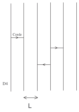
Figure 4.2: Parallel D4-branes separated by a distance of the order of $L$ with strings stretching from one to another.

As previously seen, much can be deduced from an analysis of low-energy SUGRA solutions. However, when several, say $n$, identical D-branes coincides (i.e. they are closely spaced, $L\sim\ell_{s}$) a typically stringy effect appears: the worldvolume theory gauge group is enhanced to $U(n)$. This results from the appearance of extra massless degrees of freedom corresponding to the open strings stretching between different D$p$-branes. The theory becomes a non-Abelian gauge theory which is not yet fully understood. We will briefly come back to this issue in section 7.1.

Chapter 5 BRST quantization of duality-symmetric Maxwell’s theory

The quantization of theories containing chiral $p$-forms has been already performed for several values of $p$ and different formulations of the systems. The covariant Hamiltonian BRST (Becchi-Rouet-Stora-Tyutin) quantization of one chiral boson was realized in [88] and generalized to chiral $p$-forms in [109], applying the formulation of infinitely many ghosts. On the other hand, chiral $2$–forms in $6$ dimensions have been recently quantized [110, 111] within the covariant Batalin-Vilkovisky (BV) treatment making use of various gauge-fixing conditions. The BV method has been also adopted [112] in proving the quantum equivalence of the non-covariant [87] and the Maxwell [92, 93] theories. Nevertheless, the generating functionals derived in [112] do not exhibit a manifest Lorentz covariance.

The present chapter presents the path-integral quantization for the covariant duality-symmetric Maxwell theory, that is the PST formulation. The presence of the auxiliary field non-polynomially coupled to the two gauge potentials makes the gauge algebra non-Abelian, with field-dependent structure functions. As a consequence, we must choose a suitable quantization procedure. The antifield-BRST method [113] is considered here because it is a powerful quantization technique applicable also for models with open and/or non-Abelian (field-dependent) algebras. This approach resides in compensating all the (commuting) gauge symmetries of the original system by some (fermionic) variables, called ghosts. After extending the action to a suitable chosen non-minimal sector, we have to fix the gauge. We are able to perform two different gauge-fixings [12]. The covariant one preserves Lorentz invariance but it has the disadvantage of an intricate form in the ghost sector which makes its integration difficult. On the other hand, giving up explicit Lorentz symmetry we present also a non-covariant gauge which has a simple structure in its fermionic part leading us the (formal) equality of the generating functional of PST action with the non-covariant action.

In section 5.1, we briefly illustrate the duality symmetry concepts in its most simple realization: the good old harmonic oscillator. The Hamiltonian BRST gauge-fixing of Maxwell’s action is performed in section 5.2. This shows that the generating functional of Maxwell’s theory is equal to its non-covariant (Hamiltonian) but duality-symmetric formulation, which proves their quantum equivalence [112]. In section 5.3 we compute the minimal solution of the master equation corresponding to the four-dimensional PST action. We also infer the BRST symmetry. By a well chosen non-minimal sector and an adequate gauge-fixing fermion the remaining gauge invariances are fixed. The non-covariant gauge is the starting point in proving that the generating functional of the PST and non-covariant formulations of duality-symmetric Maxwell’s theory are formally equal [10]. The latter is quantum mechanically equivalent to the ordinary Maxwell theory, so that all these models are physically related (on-shell) at the classical and quantum level, even if their off-shell descriptions are different. Still, we perform a “formal” path integral quantization in the sense that the possible UV divergences due to the non-Gaussian character of the integral were not considered. Incidentally, the absence of anomalies and non-trivial counterterms has been shown recently in [114] by power counting argument. On this basis, it seems that the PST model can be trusted at the quantum level also.

5.1 Quantum oscillator

5.1.1 Harmonic oscillator

The good old harmonic oscillator is a gentle toy model which shares analogous properties to duality symmetric electrodynamics. For instance, its manipulation suggests a convenient track to follow for Maxwell’s theory.

The harmonic oscillator Schrödinger equation kernel is equal to

$$<q_{2},t_{2}|q_{1},t_{1}>=\int{\cal D}q\,{\cal D}p\,\exp\left(i\int_{t_{1}}^{t_{2}}dt\,[p(t)\dot{q}(t)-H\left(q(t),p(t)\right)]\right)$$ (5.1.1)

where the Hamiltonian is

$$H(q,p)=\frac{1}{2}\,p^{2}+\frac{1}{2}\,q^{2}\,.$$ (5.1.2)

The boundary conditions are in the configuration space: $q(t_{1})=q_{1}$ and $q(t_{2})=q_{2}$. In the same way, in momentum space the kernel is equal to the path integral

$$<p_{2},t_{2}|p_{1},t_{1}>=\int{\cal D}q\,{\cal D}p\,\exp\left(i\int_{t_{1}}^{t_{2}}dt\,[-q(t)\dot{p}(t)-H\left(q(t),p(t)\right)]\right)$$ (5.1.3)

with boundary conditions: $p(t_{1})=p_{1}$ and $p(t_{2})=p_{2}$. In other words, the quantum harmonic oscillator Hamiltonian is invariant under the “duality” transformation

$$q \rightarrow -p,$$

$$p \rightarrow \,\,q,$$ (5.1.4)

and kernel (5.1.1) goes into kernel (5.1.3). This configuration-momentum space duality of the harmonic oscillator could seem pretty trivial, nevertheless, the electric-magnetic duality is (in some sense) nothing else than its generalization for Abelian gauge field theory. Indeed, in the Hamiltonian formalism the electric field ${\bf E}$ is “conjugate” to the magnetic field ${\bf B}$, and the Hamiltonian density $\frac{1}{2}\,({\bf E}^{2}+{\bf B}^{2})$ has the quadratic form (5.1.2).

The (classical) Hamiltonian equations are

$$\dot{q}-p=0\,,\quad\dot{p}+q=0\,.\quad$$ (5.1.5)

They are left invariant by the “duality rotation”

$$q \rightarrow \,\,\cos\alpha\,q-\,\sin\alpha\,p,$$

$$p \rightarrow -\,\sin\alpha\,q+\cos\alpha\,p.$$ (5.1.6)

Moreover, the Hamiltonian itself is manifestly invariant under this rotation. This is natural since the duality symmetry is essentially Hamiltonian in nature. We already met this fact when we looked for manifestly duality-symmetric actions. The duality rotation is a canonical transformation generated by $qp$.

To make a connection with Maxwell’s theory, we take a look at the Lagrangian formalism. The Green functions generating functional is

$$Z[J]=\int{\cal D}q\,\exp\left(i\int dt[L\left(q(t)\right)+J(t)q(t)]\right)$$ (5.1.7)

where

$$L(q)=\frac{1}{2}\,\dot{q}^{2}-\frac{1}{2}\,q^{2}\,.$$ (5.1.8)

The boundary conditions are $q(t_{1}\rightarrow-\infty)=0$ and $q(t_{2}\rightarrow+\infty)=0$. The Euler-Lagrange equation derived from (5.1.8) is

$$\ddot{q}+q=0\,.$$ (5.1.9)

We have

$$Z[J]=Z[0]\,\exp\left(\frac{-i}{2}\int dt\,dt^{\prime}\,J(t)\Delta(t-t^{\prime})J(t^{\prime})\right)$$ (5.1.10)

where

$$\Delta(t-t^{\prime})=\frac{1}{2\pi}\int\limits_{-\infty}^{+\infty}d\omega\,\frac{e^{-i\omega(t-t^{\prime})}}{\omega^{2}-1+i\epsilon}$$ (5.1.11)

To go back to a first order formalism, we can insert

$$\int{\cal D}p\,\exp\left(-\frac{i}{2}\int dt\,(p-\dot{q})^{2}\right)=const,$$ (5.1.12)

in the path integral, and get

$$Z[0]=\int{\cal D}q\,{\cal D}p\,\exp\left(i\int dt\,[p(t)\dot{q}(t)-H\left(q(t),p(t)\right)]\right)$$ (5.1.13)

with supplementary boundary conditions $p(t_{1}\rightarrow-\infty)=0$ and $p(t_{2}\rightarrow+\infty)=0$. If we integrate by part the kinetic term and use

$$\int{\cal D}q\,\exp\left(-\frac{i}{2}\int dt\,(\dot{p}-q)^{2}\right)=const.$$ (5.1.14)

we arrive at the dual formulation

$$Z[0]=\int{\cal D}p\,\exp\left(i\int dtL\left(p(t)\right)\right)\,,$$ (5.1.15)

which is exactly identical to the original one as previously stated.

As we will see in the sequel, the Maxwell theory possesses two significant new features: it is a

• Linear field theory; hence its dynamics is described by an infinite set of decoupled harmonic oscillators.

• Gauge theory; i.e. it is a system with constraints and we need to gauge-fix the action in the path integral.

In this picture non-linear electrodynamics or Yang-Mills theories appear as sophisticate systems of coupled anharmonic oscillators, which make them difficult to study outside the scope of perturbative treatment. Unfortunately, many of the beautiful mathematical results on EM duality concerns the analogue of harmonic oscillators because we mainly deal with free (= quadratic) theories. A seductive conjecture is that some (unknown) duality symmetry exists for self-interacting systems with non-Abelian gauge symmetries, like Yang-Mills theories. We will address this question in chapter 7.

5.1.2 Anharmonic oscillator

By the way, as we have seen previously with electrodynamics, some results can be generalized to some extent for non-linear theories. Presently, one can consider a general Lagrangian $L(q,\dot{q})$ and look for a necessary condition leading to a duality rotation invariant Hamiltonian: $H(q,p)=h(q^{2}+p^{2})$. The variation of the Legendre transform of the Lagrangian under an infinitesimal duality rotation is asked to vanish

$$\delta H=\delta p\,\dot{q}-\delta q\frac{\partial L}{\partial q}=0\quad\Leftrightarrow\quad q\dot{q}+\frac{\partial L}{\partial q}\frac{\partial L}{\partial\dot{q}}=0\,.$$ (5.1.16)

We recognize the Courant Hilbert equation (2.5.26) if we define $u_{+}\equiv\frac{1}{2}\dot{q}^{2}$, $u_{-}\equiv-\frac{1}{2}q^{2}$, $f(u_{+},u_{-})\equiv L\left(q(u_{+},u_{-}),\dot{q}(u_{+},u_{-})\right)$. The configuration-momentum duality symmetry will also hold for the quantum dynamics of models satisfying the equation (5.1.16). A specific example is provided by the BI-like oscillator of Lagrangian

$$L=\frac{1}{b}\left(1-\sqrt{\left(1-b\,\dot{q}^{2}\right)\left(1+b\,q^{2}\right)}\right)$$ (5.1.17)

arising from the solution (2.5.28) of the Courant Hilbert equation, where we defined $b=\frac{\alpha}{2}$. Its corresponding Hamiltonian is given by

$$H=\frac{1}{b}\left(\sqrt{1+b\,(p^{2}+q^{2})}-1\right)\,.$$ (5.1.18)

The following proposition also proves that there exists an infinite class of physically interesting duality-symmetric anharmonic oscillators.

Proposition 5.1.

Let $f(u_{+},u_{-})$ be a solution of: $f_{+}f_{-}=1$. The function $L(q,\dot{q})\equiv f\left(u_{+}(q,\dot{q}),u_{-}(q,\dot{q})\right)$

• is analytic near $(q,\dot{q})=(0,0)$ and

• satisfies $L(q,\dot{q})=\frac{1}{2}(\dot{q}^{2}-q^{2})+O(q^{4},\dot{q}^{4})$,

if and only if the Legendre transform $h(q^{2}+p^{2})\equiv pdot{q}-L(x(q,\dot{q}),y(q,\dot{q}))$, where $p=\frac{\partial L}{\partial\dot{q}}$ defines implicitly $\dot{q}(q,p)$, is such that the function $h(z)$

• is analytic near the origin $z=0$ and

• satisfies $h(z)=\frac{1}{2}z+O(z^{2})$.

Furthermore, if $h(z)$ is strictly increasing (i.e. $h^{\prime}(z)\neq 0$) then the boundary condition defines the Hamiltonian: $L(q,0)\equiv-h(q^{2})$.

• First of all, the Courant Hilbert equation (2.5.26) is a necessary and sufficient requirement to have a duality-invariant Hamiltonian $H(q,p)\equiv p\,\dot{q}-L(q,\dot{q})$.

  The dynamical system is has no constraint by hypothesis. Indeed, the two functions $p(q,\dot{q})$ and $\dot{q}(q,p)$ are invertible and are inverse of each other

  $$p=\frac{\partial L}{\partial\dot{q}}\quad\Leftrightarrow\quad\dot{q}=\frac{\partial H}{\partial p}\,.$$ (5.1.19)

  This comes from the fact that, at the origin $\frac{\partial^{2}L}{\partial\dot{q}^{2}}=1\neq 0$ and $\frac{\partial^{2}H}{\partial p^{2}}=1\neq 0$, due to the hypotheses of the proposition 5.1. From standard theorems on implicit functions [47] we find also that the two functions $p(q,\dot{q})=\dot{q}+O(q^{2},\dot{q}^{2})$ and $\dot{q}(q,p)=p+O(q^{2},p^{2})$ are analytic near the origin.

  $\underline{\,\bf\Rightarrow:}$

  We first prove the necessity. The composition of two analytic functions in a neighborhood is also an analytic function (in the corresponding neighborhood). Since $\dot{q}(q,p)=p+O(q^{2},p^{2})$ and $L(q,\dot{q})=\frac{1}{2}(\dot{q}^{2}-q^{2})+O(x,y)$ are analytic near the origin, the Hamiltonian $H(q,p)=\frac{1}{2}(q^{2}+p^{2})+O(q^{4},p^{4})$ is analytic near the origin $(q,p)=(0,0)$.

  Furthermore, since $f$ is a solution of $f_{+}f_{-}=1$ we know that the Hamiltonian is duality-invariant: $H(q,p)=h(p^{2}+q^{2})$. Therefore the function $h(z)=z+O(z^{2})$ is analytic near $z=0$.

  When $q\neq 0$, the variables $y$ vanishes if and only if $\dot{q}=0$. If $p$ vanishes, then also does $\dot{q}$ since $\dot{q}=2p\,h^{\prime}(p^{2}+q^{2})$. Conversely, if $h^{\prime}(z)\neq 0$ then $\dot{q}=0$ implies $p=0$ for consistency, which proves $L(q,0)\equiv-h(q^{2})$.

  $\underline{\,\bf\Leftarrow:}$

  By the same argument than before one proves that the function $L(q,\dot{q})=\frac{1}{2}(\dot{q}^{2}-q^{2})+O(q^{4},\dot{q}^{4})$ is analytic near the origin (with the appropriate behaviour).

  ∎

In general, it is untractable to write a Lagrangian path integral corresponding to a duality rotation invariant Hamiltonian: $H=h(q^{2}+p^{2})$ because the explicit integration over the momentum $p$ is rather awkward for an arbitrary function $h$. One has to resort to approximate methods because the classical Lagrangian receives quantum corrections, as follows from the stationary phase method (e.g. see [115], pp.344-346). Fortunately, it is easy compute the energy spectrum in the Fock basis for a duality-invariant anharmonic oscillator. First, one introduces the destruction and creation operators

$$a=\frac{1}{2}(x+ip)\,,\quad a^{+}=\frac{1}{2}(x-ip)\,.$$ (5.1.20)

Second, one defines the operator

$$N=a^{+}a=\frac{1}{2}(x^{2}+p^{2}-1)\,,$$ (5.1.21)

the spectrum of which is known to be $\mathbb{N}$ if there exists a lowest state $|0>$, the “vacuum”. Thus the energy spectrum of the duality-symmetric anharmonic oscillator is given by the formula

$$E_{n}=h(2n+1)\,,\quad n\in{\mathbb{N}}\,.$$ (5.1.22)

As an example, for the BI-like oscillator defined by the Lagrangian (5.1.17) its energy spectrum is read directly from (5.1.18):

$$E_{n}=\frac{1}{b}\left(\sqrt{2b\,n+(b+1)}-1\right)\,.$$ (5.1.23)

For large $n$, the energy levels go as $\sqrt{n}$ while they go as $n$ for the harmonic oscillator.

5.2 Hamiltonian BRST gauge-fixing of Maxwell’s action

As a warm-up, let us start with Maxwell’s theory in its standard form, i.e. non-manifestly covariant. This rather standard exercise will reveal useful by itself (i) in providing a better understanding of duality symmetry in its most natural (= Hamiltonian) formulation and (ii) in deriving the correct path integral measure from the Hamiltonian formalism (the most foolproof treatment of gauge systems).

We review the standard Hamiltonian BRST procedure by a direct glance at this specific example. Most of the material presented in the two next subsections is taken from [115], chapter 19.

5.2.1 Hamiltonian analysis

The sourceless Maxwell action (2.1.2) is equal to

$$S^{M}=-\frac{1}{4}\int d^{4}x\,F^{\mu\nu}F_{\mu\nu}\,.$$ (5.2.1)

The action is left invariant by the gauge transformations

$$\delta A_{\mu}=\partial_{\mu}\epsilon$$ (5.2.2)

The canonical momenta are

$$\pi^{0}=0\,\quad\pi^{i}=F^{i0}=-E^{i}\,,$$ (5.2.3)

$$\{A_{\mu}(\bf{x}),\pi^{\nu}(\bf{x}^{\prime})\}=\delta^{\nu}_{\mu}\,\delta(\bf{x}-\bf{x}^{\prime})$$ (5.2.4)

where $i$, $j$, $\dots$ stand for spatial indices in the 3 dimensional hyperplane $x^{0}$ constant and $\{\,,\,\}$ is the canonical Poisson bracket.

The canonical Hamiltonian $H_{C}$ (only well-defined on the submanifold defined by the primary constraint $\pi^{0}\approx 0$) is given by

$$H_{C}=H_{0}-\int d^{3}x\,A_{0}\,\partial_{i}\pi^{i}$$ (5.2.5)

where $H_{0}=\int d^{3}x\,{\cal H}_{0}$. The Hamiltonian density ${\cal H}_{0}$ is equal to

$${\cal H}_{0}=\frac{1}{2}(\pi^{i}\pi_{i}+B^{i}B_{i})\,.$$ (5.2.6)

The consistency condition $\dot{\pi}^{0}\approx 0$ leads to the secondary constraint

$$\{\pi^{0},H_{C}\}=\partial_{i}\pi^{i}\approx 0\,,$$ (5.2.7)

which one recognizes as the Gauss law $\partial_{i}E^{i}=0$. There is no further constraint. The two constraints are first class, they generate the gauge transformations (5.2.2).

The extended Hamiltonian $H_{E}$ reads

$$H_{E} = H_{C}+\int d^{3}x(\lambda\,\pi^{0}+\mu\,\partial_{i}\pi^{i})$$ (5.2.8)

$$= H_{0}+\int d^{3}x(\lambda\,\pi^{0}+\mu^{\prime}\,\partial_{i}\pi^{i})\,,$$

where $\lambda$, $\mu$ and $\mu^{\prime}$ play the role of Lagrange multiplier for the constraints. The extended Hamiltonian generates the time evolution and exhibits all the degrees of freedom in the equations of motion. In the present case, the equations contain indeed two arbitrary functions of time corresponding to the two first class constraints.

5.2.2 BRST charge and cohomology

The central idea of the BRST scheme is to replace the original gauge symmetries by a fermionic rigid symmetry acting on an appropriately extended phase space, enlarged by the “ghosts”.

For each first class constraint, we introduce a ghost: $\bar{c}$ corresponds to $\pi^{0}\approx 0$ and $c$ corresponds to the Gauss law. Their respective momenta are $\bar{\cal P}$ and $\cal P$. The Poisson bracket is extended to a (graded) bracket by the relations

$$\{\bar{c}(\bf{x}),\bar{\cal P}(\bf{x}^{\prime})\}=\delta(\bf{x}-\bf{x}^{\prime})\,,\quad\{c(\bf{x}),{\cal P}(\bf{x}^{\prime})\}=\delta(\bf{x}-\bf{x}^{\prime})\,.$$ (5.2.9)

A conventional distinction can be drawn between what is called the minimal and non-minimal sectors. The minimal sector is usually taken to be the conjugate pairs $(A_{i},\pi^{i})$ and $(c,{\cal P})$. The addition of the conjugate pairs $(A_{0},\pi^{0})$ $(\bar{c},\bar{\cal P})$ provides the non-minimal sector. This distinction arises naturally if one considers that $A_{0}$ plays the role of a Lagrange multiplier for the Gauss law in the canonical Hamiltonian (5.2.6).

The different gradings of the non-minimal sector of fields, ghosts and their momenta dictated by the set of first class constraints is listed in Table 5.1.

field & ghosts	$A_{\mu}$	$\bar{c}$	$c$	$\pi^{\mu}$	$\bar{\cal P}$	${\cal P}$
pure ghost	$0$	$1$	$1$	$0$	$0$	$0$
antighost	$0$	$0$	$0$	$0$	$1$	$1$
statistic	$+$	$-$	$-$	$+$	$-$	$-$

Table 5.1: Pure ghost number, antighost number and statistics of the (non-minimal) extended phase space.

The ghost number is defined to be the difference between the pure ghost number and the antighost number.

The BRST charge is found to be

$$\Omega=\int d^{3}x\,(\partial_{i}\pi^{i}c-i\,{\bar{c}}\,\pi_{0}).$$ (5.2.10)

Its ghost number is equal to one. It fulfills

$$\{\Omega,\Omega\}=0$$ (5.2.11)

The BRST transformation is the canonical transformation $s\,\cdot=\{\cdot,\Omega\}$. From the Jacobi identity, the equation (5.2.11) is equivalent to the nilpotency of the BRST operator, $s^{2}=0$.

The (classical) cohomology of the BRST differential is easily worked out if one introduces the transverse and longitudinal components of $A_{i}$ and $\pi^{i}$ according to the general decomposition of a vector $Z_{i}=\partial_{i}Z^{L}+Z_{i}^{T}$

$$Z_{i}^{T}=Z_{i}-\partial_{i}\bigtriangleup^{-1}(\partial_{j}A^{j})\,,\quad Z^{L}=\bigtriangleup^{-1}(\partial_{j}A^{j})\,,$$ (5.2.12)

where $\bigtriangleup^{-1}$ is the inverse Laplace operator. The BRST symmetry takes then a form where all the contractible pairs are manifest

$$sA^{L}=c\,,\quad sc=0\,, s{\cal P}=-\pi^{L}\,,\quad s\pi^{L}=0\,,$$

$$sA_{0}=-i\bar{c}\,,\quad s\bar{c}=0\,, s\bar{\cal P}=-i\pi^{0}\,,\quad s\pi^{0}=0\,,$$

$$sA_{i}^{T}=0\,, s\pi_{i}^{T}=0\,.$$ (5.2.13)

Therefore the BRST cohomology $H(s)$ is only non-trivial in vanishing ghost number, the set of observables, and is the space of functions on the reduced phase space, that is the quotient of the constraint surface by the gauge orbits, which is generated by the (two) conjugate pairs $(A_{i}^{T},\pi_{i}^{T})$.

The previous non-minimal set of ghosts and momenta is necessary to implement the covariant Lorentz gauge. However, for later use we will consider the Coulomb gauge. To go to the temporal gauge, we will make use of a singular change of variable.

5.2.3 Path integral quantization of Maxwell’s theory

For the parallel with the next section, we explicitly treat our two favorite gauge-choices: the Lorentz and Coulomb gauges.

The generating functional for the Maxwell theory in the Hamiltonian approach can be obtained from

$$Z[0]=\int{\cal D}A_{\mu}\,{\cal D}\pi^{\mu}\,{\cal D}c\,{\cal D}{\cal P}\,{\cal D}\bar{c}\,{\cal D}\bar{\cal P}\,\exp iS^{M}_{\Psi}$$ (5.2.14)

The Hamiltonian gauge-fixed action is given by

$$S^{M}_{\Psi}=\int d^{4}x\,(\pi^{\mu}\dot{A}_{\mu}+{\cal P}\dot{c}+\bar{\cal P}\dot{\bar{c}}-{\cal H}_{0}-\{\Psi,\Omega\})$$ (5.2.15)

where the function $\Psi$ is the gauge-fixing fermion ($gh(\Psi)=-1$). The gauge fixed Hamiltonian density is the sum of the gauge-fixing term $\{\Psi,\Omega\}$ and the density of the BRST-invariant extension of the extended Hamiltonian in the multiplier gauge $\lambda=\mu^{\prime}=0$ (In that case, it is simply equal to ${\cal H}_{0}$ since $\{H_{0},\Omega\}=0$). It generates a nonambiguous time evolution in the extended phase space with no arbitrariness once the gauge-fixing fermion $\Psi$ is chosen.

The Fradkin-Vilkovisky theorem ensures that the path integral is independent on the choice of gauge-fixing fermion if the boundary conditions select definite physical states at the endpoints (in such a way that the path integral stands for an expectation value between physical states). Moreover, the path integral associates well-defined (gauge choice independent) quantum average to all the BRST invariant functions of the extended phase space that belong to the same BRST cohomological class ([115], chapter 16). In other words, a change of $\Psi$ does not modify the dynamics of the BRST-invariant functions at the cohomological level.

Lorentz gauge-fixing

The gauge-fixing fermion corresponding to the Lorentz gauge is given by

$$\Psi=i\,\bar{\cal P}\,\partial_{i}A^{i}+{\cal P}A_{0}$$ (5.2.16)

With such a choice, the gauge-fixed Hamiltonian density reads

$${\cal H}={\cal H}_{0}-A_{0}\partial_{i}\pi^{i}-\pi_{0}\partial^{i}A_{i}-i{\cal P}\bar{c}+i\bar{\cal P}\bigtriangleup c\,.$$ (5.2.17)

One can easily integrate the fields $\pi^{0}$, the conjugate momenta ${\cal P}$, $\bar{\cal P}$ as well as their corresponding ghosts $c$, $\bar{c}$. Then, we obtain that

$$Z[0]=\int{\cal D}A_{\mu}\,{\cal D}\pi^{i}\,{\rm det}(\Box)\,\delta(\partial^{\mu}A_{\mu})\,\exp i{\tilde{S}}^{M}_{\Psi}$$ (5.2.18)

with

$${\tilde{S}}^{M}_{\Psi}=\int d^{4}x\,(\pi^{i}\dot{A}_{i}-{\cal H}_{0}-A_{0}\partial_{i}\pi^{i}).$$ (5.2.19)

The integration on $\pi_{0}$ gives the delta-function enforcing the Lorentz gauge while the determinant of the d’Alembert operator $\Box$ comes from the integration on the fermionic ghosts and momenta.

A last (Gaussian) integration over $\pi^{i}$ leads to a Lagrangian generating functional that could have been derived á la Fadeev-Popov (see Faddeev formula in [115], chapter 16)

$$Z[0]=\int{\cal D}A_{\mu}\,{\rm det}(\Box)\,\delta(\partial^{\mu}A_{\mu})\,\exp iS^{M}\,.$$ (5.2.20)

The Maxwell action $S^{M}$ is given in (5.2.1). One can completely eliminate the momenta in the gauge-fixed action, the terminology is that it is a “propagating gauge”.

Coulomb gauge-fixing

We will now follow the road chosen in [112] to make a connection with the non-covariant duality-symmetric formulation of Maxwell’s theory. We will first implement the Coulomb gauge in the path integral and then we will solve the Gauss law in terms of a new potential vector.

One starts by redefining the gauge-fixing function in the following way

$$\partial_{i}A^{i}\rightarrow\frac{1}{\epsilon}\,\partial_{i}A^{i}\,.$$ (5.2.21)

At the same time one performs the following field redefinition

$$\pi^{0}\rightarrow\epsilon\pi^{0}\,,\quad\bar{\cal P}\rightarrow\epsilon\bar{\cal P}\,,$$ (5.2.22)

which is of trivial(=1) super-Jacobian. The gauge-fixing fermion (5.2.16) is not modified by this change of variable. One can now get rid of the kinetic term containing $\pi^{0}$ by taking the limit $\epsilon\rightarrow 0$.

One easily integrates the field $A_{0}$ and then, as before, one integrates $\pi^{0}$, the conjugate momenta ${\cal P}$, $\bar{\cal P}$ as well as their corresponding ghosts $c$, $\bar{c}$. After all this one finds

$$Z[0]=\int{\cal D}A_{i}\,{\cal D}\pi^{i}\,{\rm det}(\Box)\,\delta(\partial_{i}\pi^{i})\,\delta(\partial^{i}A_{i})\,\exp iS_{\Psi}$$ (5.2.23)

with

$$S_{\Psi}=\int d^{4}x\,(\pi^{i}\dot{A}_{i}-{\cal H}_{0}).$$ (5.2.24)

The integration on $A_{0}$ and $\pi^{0}$ gave the delta-functions enforcing, respectively, the Gauss law and the Coulomb gauge.

The previous field redefinition and limit process is a trick which works for any internal gauge symmetries (= constraints linear and homogeneous in the momenta) to get the reduced phase space path integral (see [115], p.398) from the non-minimally extended BRST path integral. More accurately, in our case we get

$$Z[0]=\int{\cal D}A^{T}_{i}\,{\cal D}\pi^{T\,i}\,{\rm det}^{2}(\bigtriangledown)\,{\rm det}(\Box)\,{\rm det}^{-2}(\bigtriangleup)\,\exp i\tilde{S}_{\Psi}$$ (5.2.25)

with

$$\tilde{S}_{\Psi}=\int d^{4}x\,\left(\pi^{T\,i}\dot{A}^{T}_{i}-{\cal H}_{0}(A^{T}_{i},\pi^{T\,i})\right)\,$$ (5.2.26)

since the Jacobian of $Z_{i}=\partial_{i}Z^{L}+Z_{i}^{T}\rightarrow(Z^{L},Z_{i}^{T})$ is equal to $\det(\nabla)$ and

$$\delta(\partial_{i}Z^{i})=\delta(\triangle Z^{L})={\rm det}^{-1}(\bigtriangleup)\,\delta(Z^{L})\,.$$ (5.2.27)

Duality-invariant gauge-fixed path integral

In order to make the connection with the gauge-fixed duality-symmetric action, we have to move to a two-potential formulation. For this purpose, we solve the Gauss constraint $\partial_{i}\pi^{i}=0$ by introducing a potential $Z^{i}$ such that

$$\pi^{i}=\epsilon^{ijk}\partial_{j}Z_{k}.$$ (5.2.28)

The potential $Z_{i}$ can be decomposed into a sum of a longitudinal and a transverse part: $Z_{i}=Z_{i}^{L}+Z_{i}^{T}$. When $Z_{i}$ is transverse ($Z_{i}=Z^{T}_{i}$), the equation (5.2.28) is invertible (with appropriate boundary conditions). More precisely, in that case one expresses $Z_{i}$ as

$$Z_{i}=-\bigtriangleup^{-1}(\epsilon_{ijk}\partial^{j}\pi^{k})\,.$$ (5.2.29)

We can introduce the field $Z^{i}$ in the path integral in the following way

$$Z[0]=\int{\cal D}A_{i}\,{\cal D}\pi^{i}\,{\cal D}Z_{i}\,{\rm det}(\Box)\,\delta(\partial_{i}\pi^{i})\,\delta(\partial^{i}A_{i})\,\delta(Z^{i}+\bigtriangleup^{-1}\epsilon^{ijk}\partial_{j}\pi_{k})\,\exp i{\tilde{S}}^{M}_{\Psi}\,.$$ (5.2.30)

In order to make the comparison with the non-covariant approach we will use the relation

$$\delta(Z^{i}+\bigtriangleup^{-1}\epsilon^{ijk}\partial_{j}\pi_{k})=\delta(Z^{L\,i})\delta(Z^{T\,i}+\bigtriangleup^{-1}\epsilon^{ijk}\partial_{j}\pi_{k})\,.$$ (5.2.31)

We also notice that

$$\delta(Z^{T\,i}+\bigtriangleup^{-1}\epsilon^{ijk}\partial_{j}\pi_{k})\,=\,\underbrace{{\rm det}^{-1}\,(\bigtriangleup^{-1}{\rm curl})}_{={\rm det}({\rm curl})}\,\delta(\pi^{T\,i}-\epsilon^{ijk}\partial_{j}Z^{T}_{k})$$

where “${\rm curl}$” stands for the operator $\epsilon^{ijk}\partial_{j}\,,$ and $\partial_{i}\pi^{T\,i}=0$. Indeed, ${\rm det}(\bigtriangleup)={\rm det}^{2}({\rm curl})$.

In addition we have the relation

$$\delta(\partial_{i}\pi^{i})\delta(Z^{L\,i})=\delta(\pi^{L\,i})\delta(\partial_{i}Z^{i}).$$ (5.2.32)

We finally identify the two potentials as follows

$$A^{1}_{i}=A_{i}\,,\quad A^{2}_{i}=Z_{i}.$$ (5.2.33)

Putting all these remarks together we can integrate out the $\pi_{i}$ to obtain the non-covariant duality-symmetric generating functional found in [112]

$$Z[0]=\int{\cal D}A^{\alpha}_{i}\,{\rm det}(\Box)\,{\rm det}({\rm curl})\,\delta(\partial^{i}A^{\alpha}_{i})\,\exp iS^{non-cov}\,,$$ (5.2.34)

where $S^{non-cov}$ is given in the equation (4.2.12).

5.3 Batalin-Vilkovisky quantization of PST action

5.3.1 Gauge symmetries of the classical action

We start our discussion by considering the PST action proposed to manifestly implement two symmetries in the description of free Maxwell’s theory: Lorentz invariance and electric-magnetic duality. Since we are interested in studying the gauge invariances for a system with this two symmetries we will neglect here a possible supersymmetrization of the model which can be attained through a kinetic fermionic contribution of type $i{\bar{\psi}}\hbox{\ooalign{$\displaystyle\partial$\cr$/$}}\psi$ in the Lagrangian. After fixing the notation, we emphasize the physical content of this model. Next, we briefly present its gauge algebra.

The sourceless PST action [93] constructed for the description of self-dual vector field is

$$S_{0}=\int d^{4}x\left(-{1\over 8}F^{\alpha}_{\mu\nu}F^{\alpha\,\mu\nu}+{1\over{4(-u_{\lambda}u^{\lambda})}}u^{\mu}{\cal F}^{\alpha}_{\mu\nu}{\cal F}^{\alpha\,\nu\rho}u_{\rho}\right)\,.$$ (5.3.1)

As explained before the Lagrangian contains two gauge potentials $(A_{\mu}^{\alpha})_{\alpha=1,2}$ and one auxiliary field $a$, appearing here only as the gradient $u_{\mu}=\partial_{\mu}a$. The notation used throughout this paper is

$$u^{2}=u^{\mu}u_{\mu}\,,\quad\quad v_{\mu}=\frac{u_{\mu}}{\sqrt{-u^{2}}}\,,$$ (5.3.2)

$$F^{\alpha}_{\mu\nu}=2\partial_{[\mu}A^{\alpha}_{\nu]}\,,\quad\quad*F^{\alpha}_{\mu\nu}=\frac{1}{2}\epsilon_{\mu\nu\rho\sigma}F^{\alpha\,\rho\sigma}\,,$$ (5.3.3)

$${\mathcal{F}}^{\alpha}_{\mu\nu}=\epsilon^{\alpha\beta}F^{\beta}_{\mu\nu}-*F^{\alpha}_{\mu\nu}\,,\quad\quad H^{(-)\alpha}_{\mu}={\mathcal{F}}^{\alpha}_{\mu\nu}v^{\nu}$$ (5.3.4)

with $\epsilon^{\alpha\beta}$ being the antisymmetric matrix of $so(2)$ with $\epsilon^{12}=+1$. The equations of motion associated to 5.3.1 read

$$\delta A_{\mu}^{\alpha} :\quad\quad \epsilon^{\mu\nu\rho\sigma}\partial_{\nu}(v_{\rho}H^{(-)\alpha}_{\sigma})=0\,,$$ (5.3.5)

$$\delta u_{\mu} :\quad\quad \frac{1}{2\sqrt{-u^{2}}}\left(H^{(-)\alpha}_{\nu}{\mathcal{F}}^{\alpha\,\mu\nu}-H^{(-)\alpha}_{\nu}H^{(-)\alpha\,\nu}v^{\mu}\right)=0\,.$$ (5.3.6)

It is straightforward to check the following gauge invariances of the action (5.3.1)

$$\delta_{I}A_{\mu}^{\alpha}=\partial_{\mu}\varphi^{\alpha}\,, \,\delta_{I}a=0\,,$$ (5.3.7)

$$\delta_{II}A_{\mu}^{\alpha}=-\epsilon^{\alpha\beta}H^{(-)\beta}_{\mu}\frac{\phi}{\sqrt{-u^{2}}}\,, \,\delta_{II}a=\phi\,,$$ (5.3.8)

$$\delta_{III}A_{\mu}^{\alpha}=u_{\mu}\varepsilon^{\alpha}\,, \,\delta_{III}a=0\,.$$ (5.3.9)

They are irreducible. Pasti-Sorokin-Tonin have shown [92, 93] that this model is in fact classically equivalent to the non-covariant action [87] describing the dynamics of a single Maxwell field. Indeed, using the equations of motion (5.3.5) we can fix the gauge degrees of freedom of (5.3.9) in such a way that the self-duality condition

$${\mathcal{F}}^{\alpha}_{\mu\nu}=0$$ (5.3.10)

is satisfied. Such a consequence of the equations of motion allows us to express one of the gauge fields $A_{\mu}^{\alpha}$ as function of the other one yielding the usual Maxwell Lagrangian (with remaining symmetry (5.3.7)) plus a contribution of $u_{\mu}$ field. Further, we remark from the second invariance (5.3.8) that $a$ is pure gauge. Another way to see that is by expressing the field equation for $a$ as a consequence of the equation of motion for $A_{\mu}^{\alpha}$. That is why $a$ can be easily fixed away using a clever gauge condition (avoiding the singularity $u^{2}=0$). So, the field $u_{\mu}$ as well as one of the two $A_{\mu}^{\alpha}$ are auxiliary in the sense that one needs them only to lift self-duality and Lorentz invariance at the rank of manifest symmetries of the action. But, they can be removed on the mass-shell taking into account the gauge invariances of the new system. The manner of fixing the unphysical degrees of freedom in the BRST formalism will be clarified in subsection 5.3.4.

For the gauge algebra we get

$$[\delta_{II}(\phi_{1}),\delta_{II}(\phi_{2})] = \delta_{III}\left(\frac{\epsilon^{\alpha\beta}H^{(-)\beta}_{\mu}}{(-u^{2})^{3/2}}(\phi_{1}\partial^{\mu}\phi_{2}-\phi_{2}\partial^{\mu}\phi_{1})\right)\,,$$ (5.3.11)

$$\left[\delta_{II}(\phi),\delta_{III}(\varepsilon^{\alpha})\right] = \delta_{I}(\phi\varepsilon^{\alpha})+\delta_{III}\left(\frac{u^{\mu}\phi}{(-u^{2})}\partial_{\mu}\varepsilon^{\alpha}\right)\,.$$ (5.3.12)

Thus, our system describes a non-Abelian gauge theory with structure constants replaced by non-polynomial structure functions.

5.3.2 Basic ingredients of antifield-BRST formalism

Here we give only some of the main ideas underlying the Lagrangian BRST method. For more details we refer the reader to [113, 115, 116, 117] and references therein).

Let $S_{0}[\phi^{i}]$ be an action with the following bosonic gauge transformations

$$\delta_{\varepsilon}\phi^{i}=R^{i}_{\alpha}\epsilon^{\alpha}$$ (5.3.13)

which are irreducible. Then, one has to enlarge the “field” content to

$$\{\Phi^{A}\}=\{\phi^{i},C^{\alpha}\}.$$ (5.3.14)

The fermionic ghosts $C^{\alpha}$ correspond to the parameters $\varepsilon^{\alpha}$ of the gauge transformations (5.3.13). To each field $\Phi^{A}$ we associate an antifield $\Phi_{A}^{*}$ of opposite parity. The set of associated antifields is then

$$\{\Phi_{A}^{*}\}=\{\phi^{*}_{i},C^{*}_{\alpha}\}.$$ (5.3.15)

The fields possess a vanishing antighost number ( antigh) and a nonvanishing pureghost number ( pgh)

$$pgh(\phi^{i})=0,\quad pgh(C^{\alpha})=1.$$ (5.3.16)

The pgh number of the antifields vanish but their respective antigh number is equal to

$$antigh(\Phi_{A}^{*})=1+pgh(\Phi^{A}).$$ (5.3.17)

The total ghost number ( gh) equals the difference between the pgh number and the antigh number. The antibracket of two functionals $X[\Phi^{A},\Phi_{A}^{*}]$ and $Y[\Phi^{A},\Phi_{A}^{*}]$ is defined as

$$(X,Y)=\int d^{n}x\left(\frac{\delta^{R}X}{\delta\Phi^{A}(x)}\frac{\delta^{L}Y}{\delta\Phi_{A}^{*}(x)}-\frac{\delta^{R}X}{\delta\Phi_{A}^{*}(x)}\frac{\delta^{L}Y}{\delta\Phi^{A}(x)}\right)\,,$$ (5.3.18)

where $\delta^{R}/\delta Z(x)$ and $\delta^{L}/\delta Z(x)$ denote functional right- and left-derivatives.

The extended action $S$ is defined by adding to the classical action $S_{0}$ terms containing the antifields coupled to the BRST variations of the fields in such a way that the classical master equation,

$$(S,S)=0\,,$$ (5.3.19)

is satisfied, with the following boundary condition:

$$S=S_{0}+\phi^{*}_{i}R^{i}_{\alpha}C^{\alpha}+...$$ (5.3.20)

This imposes the value of terms quadratic in ghosts and antifields. The extended action has also to be of vanishing gh number. If the algebra is non-Abelian, we know that we have to add other pieces of antigh number two in the extended action with the general form (due to structure functions)

$$S_{2}^{2a}=\frac{1}{2}C_{\alpha}^{*}f_{\beta\gamma}^{\alpha}C^{\beta}C^{\gamma}\,.$$ (5.3.21)

If the algebra is open, other terms in antigh number must be added, quadratic in $\phi^{*}_{i}$’s. Furthermore, other terms in higher antigh number could be necessary, e.g. when the structure functions depend on the fields $\phi^{i}$.

The extended action captures all the information about the gauge structure of the theory: the Noether identities, the (on-shell) closure of the gauge transformations and the higher order gauge identities are contained in the master equation.

The BRST transformation $s$ in the antifield formalism is a canonical transformation, i.e. $sA=(A,S)$. It is a differential: $s^{2}=0$, its nilpotency being equivalent to the master equation (5.3.19). The BRST differential decomposes according to the antigh number as

$$s=\delta+\gamma+"more"$$

and provides the gauge invariant functions on the stationary surface, through its cohomology group at gh number zero $H_{0}(s)$. The Koszul-Tate differential $\delta$ defined by

$$\delta\Phi^{*}_{i}=(\Phi^{*}_{i},S)|_{\Phi_{A}^{*}=0}$$ (5.3.22)

implements the restriction on the stationary surface, and the exterior derivative along the gauge orbits $\gamma$

$$\gamma\Phi^{i}=(\Phi^{i},S)|_{\Phi^{*}_{A}=0}$$

picks out the gauge-invariant functions.

The solution $S$ of the master equation possesses gauge invariance, and thus, cannot be used directly in a path integral. There is one gauge symmetry for each field-antifield pair. The standard procedure to get rid of these gauge degrees of freedom is to use the gauge-fixed action $S_{\Psi}$ defined by

$$S_{\Psi}=S_{non-min}\left[\Phi^{A},\Phi^{*}_{A}=\frac{\delta\Psi[\Phi^{A}]}{\delta\Phi^{A}}\right].$$ (5.3.23)

The functional $\Psi[\Phi^{A}]$ is known as the gauge-fixing fermion and must be such that $S_{\Psi}[\Phi]$ is non-degenerate, i.e. the equations of motion derived from the gauge-fixed action $\delta S_{\Psi}[\Phi^{A}]/\delta\Phi^{A}=0$ have unique solution for arbitrary initial conditions, which means that all gauge degrees of freedom have been eliminated. It also has to be local in order that the antifields be given by local functions of the fields.

The generating functional of the theory is then

$$Z=\int[{\mathcal{D}}\Phi^{A}]\exp iS_{\Psi}$$ (5.3.24)

The value of the path integral is independent of the choice of the gauge-fixing fermion $\Psi$. The notation $[{\mathcal{D}}\Phi]$ stands for ${\mathcal{D}}\Phi\,\mu[\Phi]$, where $\mu[\Phi]$ is the measure of the path integral. It is important to notice that the expression of the measure $\mu[\Phi]$ in this path integral is not completely determined by the Lagrangian approach. A correct way to determine it, would be to start from the Hamiltonian approach for which the choice of measure is trivial, indeed it is known to be ${\mathcal{D}}\Phi{\mathcal{D}}\Pi$, that is the product over time of the Liouville measure $d\Phi^{A}d\Pi_{A}$. The Hamiltonian formalism meets no problem because the Hamiltonian gauge-fixed action has no gauge invariance. It can be proved that, if correctly handled, the two approaches are equivalent (see [115] for instance). This justifies a posteriori the choice of the measure $\mu[\Phi]$ in (5.3.24).

5.3.3 Minimal solution of the master equation

Having made the classical analysis of the model, we can start now the standard BRST procedure. The first step is to construct the minimal solution of the master equation with the help of the gauge algebra. In order to reach that end we will introduce some new fields called ghosts and their antibracket conjugates known as antifields.

The minimal sector of fields and antifields dictated by the gauge invariances (5.3.7)-(5.3.9) as well as their ghost numbers and statistics are listed in Table 5.2.

$\Phi$	$A_{\mu}^{\alpha}$	$a$	$A_{\mu}^{\alpha*}$	$a^{*}$	$c^{\alpha}$	$c$	$c^{\prime\alpha}$	$c^{\alpha*}$	$c^{*}$	$c^{\prime\alpha*}$
$gh(\Phi)$	$0$	$0$	$-1$	$-1$	$1$	$1$	$1$	$-2$	$-2$	$-2$
$antigh(\Phi)$	$0$	$0$	$1$	$1$	$0$	$0$	$0$	$2$	$2$	$2$
stat($\Phi$)	$+$	$+$	$-$	$-$	$-$	$-$	$-$	$+$	$+$	$+$

Table 5.2: Ghost number, antighost number and statistics of the minimal fields and their antifields.

The transformations (5.3.7)-(5.3.9) determine directly the $antigh$ number one piece of the extended action, i.e.

$$S_{1} = \int d^{4}\,x\left[A^{\alpha*\mu}\left(\partial_{\mu}c^{\alpha}-\epsilon^{\alpha\beta}H^{(-)\beta}_{\mu}\frac{c}{\sqrt{-u^{2}}}+u_{\mu}c^{\prime\alpha}\right)+a^{*}c\right]\,.$$ (5.3.25)

In order to take into account the structure functions one has to insert in the solution of the master equation a contribution with $antigh$ number two of the form

$$S_{2}=\int d^{4}\,x\left[c^{\prime\alpha*}\left(\frac{\epsilon^{\alpha\beta}H^{(-)\beta}_{\mu}}{(-u^{2})^{3/2}}\,c\,\partial^{\mu}c+\frac{v_{\mu}}{\sqrt{-u^{2}}}\,c\,\partial^{\mu}c^{\prime\alpha}\right)+c^{\alpha*}c\,c^{\prime\alpha}\right]\,.$$ (5.3.26)

Due to the field dependence of the structure functions one should expect that $S_{1}$ and $S_{2}$ are not enough to completely determine the extended action and one will need an extra piece of $antigh$ number three to do the job. Indeed, that was already the case for chiral 2–forms in 6 dimensions discussed in [110]. Nevertheless, one can readily check that in the present situation $S_{min}=S_{0}+S_{1}+S_{2}$ is the minimal solution of the classical master equation $(S_{min},S_{min})=0$, i.e.

$$(S_{1},S_{1})_{1}+2(S_{1},S_{1})_{1}=0\,,$$

$$(S_{2},S_{2})_{2}+2(S_{1},S_{2})_{2}=0\,.$$ (5.3.27)

This follows also as a consequence of the irreducibility of our model.

Once $S_{min}$ has been derived, we can infer the BRST operator $s$, which is the sum of three operator of different antigh number

$$s=\delta+\gamma+\rho\,.$$ (5.3.28)

For instance, the non-trivial action of the Koszul-Tate differential, of antigh number $-1$, is in our case given by

$$\delta A^{\alpha*\mu} = \epsilon^{\mu\nu\rho\sigma}\partial_{\nu}(v_{\rho}H^{(-)\alpha}_{\sigma})\,,$$ (5.3.29)

$$\delta a^{*} = \partial_{\mu}\left(\frac{1}{2\sqrt{-u^{2}}}\left(H^{(-)\alpha}_{\nu}{\mathcal{F}}^{\alpha\,\mu\nu}-H^{(-)\alpha}_{\nu}H^{(-)\alpha\,\nu}v^{\mu}\right)\right)\,,$$ (5.3.30)

$$\delta c^{\alpha*} = -\partial^{\mu}A^{\alpha*}_{\mu}\,,$$ (5.3.31)

$$\delta c^{*} = -\frac{\epsilon^{\alpha\beta}H^{(-)\beta\mu}}{\sqrt{-u^{2}}}A^{\alpha*}_{\mu}+a^{*}\,,$$ (5.3.32)

$$\delta c^{\prime\alpha*} = u^{\mu}A^{\alpha*}_{\mu}\,.$$ (5.3.33)

The third piece, $\rho$, of antigh number $+1$ is present also because the structure functions determined by (5.3.7)-(5.3.9) depend explicitly on the fields.

In this way the goal of this section, i.e. the construction of the minimal solution for the master equation, has been achieved.

5.3.4 The gauge-fixed action

The minimal solution $S_{min}$ will not suffice to fix all the gauge invariances of the system and, before fixing the gauge, we need a non-minimal solution for $(S,S)=0$ in order to take into account the trivial gauge transformations. In this section we first construct such a non-minimal solution and, afterwards, we propose two possible gauge-fixing conditions which will yield two versions for the gauged-fixed action: a covariant and a non-covariant one.

Non-minimal sector

Inspired by the gauge transformations (5.3.7)-(5.3.9) and their irreducibility we propose a non-minimal sector described in Table 5.3.

$\Phi$	$B^{\alpha}$	$B$	$B^{\prime\alpha}$	${\bar{C}}^{\alpha}$	${\bar{C}}$	${\bar{C}}^{\prime\alpha}$	$B^{\alpha*}$	$B^{*}$	$B^{\prime\alpha*}$	${\bar{C}}^{\alpha*}$	${\bar{C}}^{*}$	${\bar{C}}^{\prime\alpha*}$
$gh(\Phi)$	$0$	$0$	$0$	$-1$	$-1$	$-1$	$-1$	$-1$	$-1$	$0$	$0$	$0$
stat($\Phi$)	$+$	$+$	$+$	$-$	$-$	$-$	$-$	$-$	$-$	$+$	$+$	$+$

Table 5.3: Ghost number and statistics of the non-minimal fields and their antifields.

They satisfy the following equations

$$s{\bar{C}}^{\cdots}=B^{\cdots}\,,\quad\quad sB^{\cdots}=0\,,$$

$$sB^{\cdots*}={\bar{C}}^{\cdots*}\,,\quad\quad s{\bar{C}}^{\cdots*}=0\,.$$ (5.3.34)

The dots are there to express that these relations are valid for the correspondingly three kinds of non-minimal fields. We immediately see that $\bar{C}^{\cdots}$’s and $B^{\cdots}$’s constitute trivial pairs, as well as their respective antifields, in such a way that they do not enter in the cohomology of $s$. Hence, they are called non-minimal. Their contribution to a solution of the master equation is

$$S_{non-min}=S_{min}+\int d^{4}\,x\left({\bar{C}}^{\alpha*}B^{\alpha}+{\bar{C}}^{*}B+{\bar{C}}^{\prime\alpha*}B^{\prime\alpha}\right)\,.$$ (5.3.35)

Covariant gauge fixing

We will first try a covariant gauge fixing leading in principle to a covariant gauge-fixed action: we will see what is the main problem that occurs. We can consider the following covariant gauge choices

$$\delta_{I} \rightarrow \partial^{\mu}A^{\alpha}_{\mu}=0\,,$$ (5.3.36)

$$\delta_{II} \rightarrow u^{2}+1=0\,,$$ (5.3.37)

$$\delta_{III} \rightarrow u^{\mu}A^{\alpha}_{\mu}=0\,.$$ (5.3.38)

The gauge choice (5.3.36) is analogous to the Lorentz gauge. In its turn (5.3.37) allows to take a particular Lorentz frame in which $u^{\mu}(x)$ is the unit time vector at the point $x$. In such a case, at the point $x$, (5.3.38) is the temporal gauge condition for the two potentials.

A gauge-fixing fermion corresponding to the gauge choices (5.3.36)-(5.3.38) is

$$\Psi[\Phi^{A}]=-\int d^{4}\,x\left[{\bar{C}}^{\alpha}\partial^{\mu}A^{\alpha}_{\mu}+{\bar{C}}(u^{2}+1)+{\bar{C}}^{\prime\alpha}u^{\mu}A^{\alpha}_{\mu}\right]\,.$$ (5.3.39)

We express now all the antifields with the help of $\Psi[\Phi]$, i.e.

$$\Phi^{*}_{A}=\frac{\delta\Psi[\Phi^{A}]}{\delta\Phi^{A}}$$ (5.3.40)

getting

$$A_{\mu}^{\alpha*} = \partial_{\mu}{\bar{C}}^{\alpha}-u_{\mu}{\bar{C}}^{\prime\alpha}\,,$$ (5.3.41)

$$a^{*} = 2\partial_{\mu}(u^{\mu}{\bar{C}})+\partial^{\mu}(A_{\mu}^{\alpha}{\bar{C}}^{\prime\alpha})\,,$$ (5.3.42)

$$c^{\cdots*} = 0\,,$$ (5.3.43)

$$B^{\cdots*} = 0\,,$$ (5.3.44)

$${\bar{C}}^{\alpha*} = -\partial^{\mu}A^{\alpha}_{\mu}\,,$$ (5.3.45)

$${\bar{C}}^{*} = -(u^{2}+1)\quad\quad{\bar{C}}^{\prime\alpha*}=-u^{\mu}A^{\alpha}_{\mu}\,.$$ (5.3.46)

Using the last relations we can find the gauge fixed action as in (5.3.23) which in our case reads

$$S_{\Psi} = S_{0}+\int d^{4}\,x\left[-{\bar{C}}^{\alpha}\Box c^{\alpha}-\frac{\epsilon^{\alpha\beta}H^{(-)\beta\mu}}{\sqrt{-u^{2}}}\partial_{\mu}{\bar{C}}^{\alpha}\cdot c+u^{\mu}\partial_{\mu}{\bar{C}}^{\alpha}\cdot c^{\prime\alpha}\right.$$ (5.3.47)

$$-u_{\mu}{\bar{C}}^{\prime\alpha}\partial^{\mu}c^{\alpha}-u^{2}{\bar{C}}^{\prime\alpha}c^{\prime\alpha}-(2u_{\mu}{\bar{C}}+A_{\mu}^{\alpha}{\bar{C}}^{\prime\alpha})\partial^{\mu}c$$

$$\left.-(\partial^{\mu}A^{\alpha}_{\mu})B^{\alpha}-(u^{2}+1)B-(u^{\mu}A^{\alpha}_{\mu})B^{\prime\alpha}\right]\,.$$

Writing down the path integral (5.3.24), we integrate directly the fields $B^{\cdots}$ producing the gauge conditions (5.3.36)-(5.3.38). A further integration of ${\bar{C}}$, ${\bar{C}}^{\prime\alpha}$ and $c^{\prime\alpha}$ (in this order) leads to

$$Z[0]=\int{\mathcal{D}}A^{\alpha}_{\mu}{\mathcal{D}}a{\mathcal{D}}c^{\alpha}{\mathcal{D}}c{\mathcal{D}}{\bar{C}}^{\alpha}\,\delta(\partial^{\mu}A_{\mu}^{\alpha})\,\delta(u^{2}+1)\,\delta(u^{\mu}A_{\mu}^{\alpha})\,\delta(u^{\mu}\partial_{\mu}c)\exp iS^{\prime}_{\Psi}$$ (5.3.48)

where

$$S^{\prime}_{\Psi}=\int d^{4}x\left[-{\bar{C}}^{\alpha}\Box c^{\alpha}+\left(\frac{\epsilon^{\alpha\beta}H^{(-)\beta\mu}}{\sqrt{-u^{2}}}\,c+\frac{u^{\mu}}{u^{2}}(u^{p}\partial_{p}c^{\alpha}+A_{\nu}^{\alpha}\partial^{\nu}c)\right)\partial_{\mu}{\bar{C}}^{\alpha}\right].$$ (5.3.49)

Of course, the next step in getting a covariant generating functional from which we would read out the covariant propagator for the fields $A_{\mu}^{\alpha}$ would be the elimination of $c$ and $a$ in (5.3.48). Due to the “gauge condition” for the ghost $c$ (i.e. $u^{\mu}\partial_{\mu}c=0$) and the way it enters the gauge-fixed action $S^{\prime}_{\Psi}$, this integration is technically difficult. What one could try is to integrate both $c$ and $a$ at the same time. This is also not straightforwardly possible as a consequence of the gauge condition (5.3.37). This requirement was necessary to covariantly fix the symmetry (5.3.8). Nevertheless, one can attempt to find the general solution to this equation (5.3.37), which reduces to the integration of $\partial^{\mu}a=\Lambda^{\mu}{}_{p}(x)n^{p}$ (with $\Lambda^{\mu}{}_{p}(x)$ a point-dependent Lorentz boost and $n_{p}$ a constant time-like vector, i.e. $n_{p}n^{p}=-1$). Such a solution is still unconvenient due to $x$-dependence of the Lorentz transformation matrix $\Lambda^{\mu}{}_{p}(x)$.

A way to overcome this sort of complication is to choose a particular form for this matrix, breaking Lorentz symmetry. It is precisely this price that we have to pay in order to explicitly derive the propagator of $A_{\mu}^{\alpha}$ fields. As it will be explained in the next subsection, by taking a particular solution for (5.3.37), i.e. by giving up Lorentz invariance, we will be able to express the gauged-fixed action in a more convenient form for our purposes.

Non-covariant gauge fixing

As it was remarked in the previous subsection in order to explicitly derive the Feynman rules for the PST model one has to break up its Lorentz symmetry by taking a specific solution of the equation (5.3.37). In this subsection we present a non-covariant gauge of the theory and the advantages for such a choice will become clear in the next sections. A possible non-covariant gauge fixing is

$$\delta_{I} \rightarrow \partial^{\mu}A^{\alpha}_{\mu}=0\,,$$ (5.3.50)

$$\delta_{II} \rightarrow a-n_{\mu}x^{\mu}=0\,,\quad\quad n_{\mu}n^{\mu}=-1\,,$$ (5.3.51)

$$\delta_{III} \rightarrow n^{\mu}A^{\alpha}_{\mu}=0\,.$$ (5.3.52)

By (5.3.51), the gradient $\partial^{\mu}a$ becomes equal to the vector $n^{\mu}$ introduced above. In a Lorentz frame where $n^{\mu}=(1,0,0,0)$ the requirement (5.3.52) is the temporal gauge condition and (5.3.50) the Coulomb gauge condition for the two potentials $A^{\alpha}_{\mu}$.

Then, the gauge-fixing fermion will be

$$\Psi[\Phi^{A}]=-\int d^{4}\,x\left[{\bar{C}}^{\alpha}\partial^{\mu}A^{\alpha}_{\mu}+{\bar{C}}(a-n_{\mu}x^{\mu})+{\bar{C}}^{\prime\alpha}n^{\mu}A^{\alpha}_{\mu}\right]\,.$$ (5.3.53)

Using the same non-minimal contribution $S_{non-min}$ as before, the non-covariant gauge-fixed action is

$$S_{\Psi}=S_{0} + \int d^{4}\,x\left[\left(\partial^{\mu}{\bar{C}}^{\alpha}-u^{\mu}{\bar{C}}^{\prime\alpha}\right)\left(\partial_{\mu}c^{\alpha}-\epsilon^{\alpha\beta}H^{(-)\beta}_{\mu}\frac{c}{\sqrt{-u^{2}}}+u_{\mu}c^{\prime\alpha}\right)\right.$$ (5.3.54)

$$+\left(-{\bar{C}}+\partial^{\mu}(A_{\mu}^{\alpha}{\bar{C}}^{\prime\alpha})\right)\cdot c-\partial^{\mu}A^{\alpha}_{\mu}B^{\alpha}$$

$$\left.-(a-n_{\mu}x^{\mu})B-u^{\mu}A^{\alpha}_{\mu}B^{\prime\alpha}\right]\,.$$

This action is by far more convenient in deriving the propagator of the gauge fields than its covariant expression (5.3.49) because we can completely integrate the ghost sector. Also, the bosonic part takes a more familiar form. The quantum equivalence of the PST model with ordinary Maxwell’s theory will be based also on this non-covariant action.

5.3.5 Path integral

The gauge-fixed action corresponding to the non-covariant gauge choice can be used to recover the non-covariant theory, which is itself equivalent to the Maxwell theory. The generating functional is taken to be

$$Z=\int{\cal D}A^{\alpha}_{\mu}\,{\mathcal{D}}a\,{\mathcal{D}}c^{\cdots}\,{\mathcal{D}}B^{\cdots}\,{\mathcal{D}}\bar{C}^{\cdots}\,{\rm det}(\Box)\,{\rm det}^{-1}({\rm curl})\,\exp iS_{\Psi}$$ (5.3.55)

where $S_{\Psi}$ is given by (5.3.54).

After integrating out some fields, in the following order ($B^{\cdots},$ $\bar{C},$ $c,$ $\bar{C}^{\prime\alpha},$ $c^{\prime\alpha},$ $a$), we obtain the path integral

$$Z=\int{\cal D}A^{\alpha}_{\mu}\,{\mathcal{D}}{\bar{C}}^{\alpha}\,{\mathcal{D}}c^{\alpha}\,{\rm det}(\Box)\,\,{\rm det}^{-1}({\rm curl})\,\delta(\partial^{\mu}A^{\alpha}_{\mu})\,\delta(n^{\mu}A^{\alpha}_{\mu})\,\exp iS^{\prime}_{\Psi}$$ (5.3.56)

where the gauge-fixed action reduces now to

$$S_{\Psi}^{\prime}=\int d^{4}\,x\left[-\frac{1}{2}n^{\mu}*F^{\alpha}_{\mu\nu}{\mathcal{F}}^{\alpha\,\nu\rho}n_{\rho}-{\bar{C}}^{\alpha}\Box c^{\alpha}-{\bar{C}}^{\alpha}n^{\mu}n^{\nu}\partial_{\mu}\partial_{\nu}c^{\alpha}\right]$$ (5.3.57)

If we place ourselves in a Lorentz frame where $n^{\mu}=(1,0,0,0)$, the functional $S^{\prime}_{\Psi}$ assumes the form of the sum of non-covariant gauge-fixed action (4.2.12) with a ghost term

$$-\int d^{4}x\,{\bar{C}}^{\alpha}\bigtriangleup c^{\alpha}\,.$$ (5.3.58)

At this point we can integrate out the ghosts $\bar{C}^{\alpha}$ and $c^{\alpha}$, and the two fields $A^{\alpha}_{0}$, obtaining exactly the generating functional (5.2.34) of the Maxwell theory in the non-covariant formulation (see section 5.2).

This proves a formal (quantum) equivalence of the PST action (5.3.1) with the Maxwell theory [10] which was already known at the classical level. The equality of the two generating functionals was not obvious a priori because the PST action of the free Maxwell’s theory is not quadratic (and so the path integral is not Gaussian) and the pure gauge field $a$ is not, strictly speaking, an auxiliary field (its equation of motion is not an algebraic relation which allows its elimination from the action). The absence of anomalies and non-trivial counterterms has been proved in [114] which strongly supports the true equivalence of the PST model with the Maxwell theory.

Chapter 6 Quantization conditions

Yang-Mills gauge theory in $2+1$ dimensions with a CS term (also called topological mass term) is known to have its topological mass quantized for gauge groups with a non-trivial third homotopy group [58]. In general, the CS coefficient is quantized since $\pi_{3}(G)\cong\mathbb{Z}$ for any semi-simple Lie group $G$. However, in the Abelian case with compact group manifold $G=U(1)$ all the homotopy groups higher than $\pi_{1}$ are trivial and, a priori, the CS coefficient can take arbitrary values. The authors of [63] have pointed out that when electric and magnetic charges are present the CS coefficient must also be quantized, just as in the non-Abelian case. The quantization arises from two key features. The first one is that, for non-vanishing CS coefficient, electric worldlines can end on magnetic sources, thereby relating the electric charge to the magnetic charge via the CS coefficent. The second key property is the usual Dirac charge quantization condition that was shown to remain valid in the presence of a CS term by the authors. As they noticed, their construction can be straightforwardly generalized to $p$-brane electrodynamics in $(2p+3)$-dimensional spacetime where the electric $p$-branes have the same dimensionality than the Dirac branes attached to the magnetic $(p-1)$-brane, and for which equations of motion are linear.

The next step would be to consider theories with a cubic CS term in the action. This is the subject of section 6.3. For $p$-brane electrodynamics, a cubic term exists only in $(3p+5)$-dimensional spacetime. The extended dual objects carrying magnetic charge have $2p+1$ spacelike dimensions. With a non-vanishing CS coefficient, electric branes can end on magnetic branes. A new feature is that the boundary of the electric brane creates a dyonic $(p-1)$-brane living on the worldvolume of the magnetic brane. In the cubic case, it is the electric brane and the Dirac brane attached to the dyonic brane, who shares the same dimensionality but a modified version of the previous argument [63] can provide a new quantization of the corresponding CS coefficient.

In supergravity theories, the CS coefficent is usually fixed by supersymmetry. Therefore the fact that the CS coefficient is quantized (without any help of supersymmetry) can be understood as another supporting evidence of the M-theory conjecture, since the bosonic sector of the effective quantum theory somehow “feels” supersymmetry.

6.1 Charge quantization condition

There exists such a huge number of different derivations of the charge quantization condition that we just give few examples. The most standard approach might be the Dirac’s 1948 derivation [5] based on the unobservability of the Dirac string. But there are other formulations in which one does not even need to introduce a Dirac brane: for instance, if one proceeds à la Wu-Yang [118], or if one uses the electromagnetic momentum quantization [4]. In 1968, Zwanziger derived the charge quantization condition for dyons by using the Dirac-Schwinger criterion [119, 120] to enforce Lorentz invariance [121]. Consistency under charge shifts produced by (generalized) $\theta$-terms or compactification effects were also used in [50] to derive the quantization condition for dyonic branes. Recently, it was reobtained geometrically from the classification of $p$-gerbes [31]. Here we will follow the Lagrangian path-integral approach chosen by the authors of [32, 33]. With the aim of simplicity we will work without manifest duality symmetry. For a duality-symmetric treatment we refer to [32, 33].

6.1.1 Dual branes

For simplicity, we will consider the electrodynamics for a system with a single brane only electrically charged and a single (distinct) brane only magnetically charged. We take an action inspired from section 2.5 which reads

$$S[A_{\mu_{1}\ldots\mu_{p+1}},G_{\mu_{1}\ldots\mu_{D-p-2}},J_{e}^{\mu_{1}\ldots\mu_{p+1}}]=$$

$$\quad=\int\limits_{\cal M}{\cal L}(F_{\mu_{1}\ldots\mu_{p+2}})+(-)^{D-p-1}\int\limits_{\cal M}*J_{e}\wedge A-T_{e}\int\limits_{{\cal M}_{e}}(*1)-T_{m}\int\limits_{{\cal M}_{m}}(*1)\,.$$

with the same definitions as before. Furthermore, $T_{e}$ and $T_{m}$ are the brane tensions. The Dirac brane is assumed to obey the Dirac veto. As seen in subsection 2.3, one has the following gauge freedom

$$*G\rightarrow*G+d*V\,,\quad A\rightarrow A+d\Lambda-*V\,,$$ (6.1.1)

corresponding to a change $\Delta{\cal M}_{D}=\partial{\cal V}$ in the Dirac brane, $*V=gP({\cal V})$. The variation of the action under such a large gauge transformation is equal to

$$\Delta S=(-)^{D-p}\,eg\,L({\cal M}_{e},\Delta{\cal M}_{D})\,,$$ (6.1.2)

where $L({\cal M}_{e},\Delta{\cal M}_{D})$ is the linking number between the electric brane worldvolume ${\cal M}_{e}$ and the Dirac brane variation $\Delta{\cal M}_{D}$ in the spacetime $\cal M$. As pointed earlier, since this is a topological quantity, the physics is independent of the choice of Dirac brane at the classical level. But at the quantum level, the path integral would not be invariant in general and there would be some kind of anomaly. If there exist a (purely) electric brane and a (purely) magnetic brane, quantum consistency enforces the product of the electric charge density $e$ (of unit $L^{D/2-p-2}$) with the magnetic charge density $g$ (of unit $L^{p-D/2+2}$) to be equal to a multiple of $2\pi$, i.e.

$$eg=2\pi n,\quad\quad n\in\mathbb{Z}\,.$$ (6.1.3)

This requirement is the so-called Dirac quantization condition.

Remark: There is no quantization condition if the electric and magnetic branes are in a configuration such that the variation of the Dirac brane worldvolume $\Delta{\cal M}_{D}$ cannot link around the electric charge worldvolume ${\cal M}_{e}$. An example of such a configuration is when infinite magnetic and electric branes have some common asymptotic spatial direction. Such configurations were called Dirac insensitive by the authors of [122]. As they have shown, this property is essential for consistency with Kaluza-Klein reductions.

Application in M-theory

As an example, it is known that the $F$-string and the NS$5$-brane, the dual D$p$-branes, the M$2$-brane and M$5$-brane obeys the Dirac quantization condition (remarkably, for the minimal value $|n|=1$). One of the non-trivial consistency check of the $M$-theory conjecture has been to check if they fulfill the Dirac charge quantization condition. Consistency with the web of dualities determined the BPS brane tensions in terms of the fundamental length scale (this result is reviewed in [124]).

Further, by considering the implications of consistency with $T$-duality together with some special “scale setting” (e.g. for the dyonic D$3$-brane in type IIB superstring theory), charge scales in $D\leq 10$ supergravity theories were determined without recourse to M-theory [122]. In fact the derived relations can be interpreted as supporting evidence for the M-theory conjecture.

6.1.2 Dyonic branes

We now restrict ourselves to the $p$-brane electrodynamics in $D=2p+4$ (the case $p$ even was considered in section 2.6) where dyonic branes may exist. For simplicity, let us assume that there are only two dyons of charge density $(e_{1},g_{1})$ and $(e_{2},g_{2})$, of worldvolume ${\cal M}^{2}=\partial{\cal N}^{1}$ and ${\cal M}^{1}=\partial{\cal N}^{2}$ with Dirac brane ${\cal N}^{1}$ and ${\cal N}^{2}$. One takes the following action

$$S[A_{\mu_{1}\ldots\mu_{p+1}},G^{\mu_{1}\ldots\mu_{p+2}},J_{e}^{\mu_{1}\ldots\mu_{p+1}}]=$$

$$=\int\limits_{\cal M}L(F_{\mu_{1}\ldots\mu_{2(p+1)}})+\frac{1}{2}\,\theta\int\limits_{\cal M}F\wedge F+(-)^{p+1}\int\limits_{\cal M}*J_{e}\wedge A+I_{K}$$ (6.1.4)

For $p$ odd, the $\theta$-term is not really present since $F\wedge F\equiv 0$. The variation of the action under a large gauge transformation (largeg) corresponding to a change of Dirac brane

$${\cal N}^{1}\rightarrow{\cal N}^{{}^{\prime}1}={\cal N}^{1}+\partial{\cal V}_{1}\,,\quad{\cal N}^{2}\rightarrow{\cal N}^{\prime}_{2}={\cal N}_{2}+\partial{\cal V}_{2}\,,$$ (6.1.5)

is equal to

$$\Delta S=(-)^{p}\int\limits_{\cal M}*J_{e}\wedge*V$$ (6.1.6)

Now, we use the identity $*J_{e}\wedge*V=*J^{1}_{e}\wedge*V^{2}+*J^{2}_{e}\wedge*V^{1}$ to get

$$S^{\prime}-S=(-)^{p}\left[e_{1}g_{2}\,L({\cal M}^{1},{\cal N}^{{}^{\prime}2}-{\cal N}_{2})+e_{2}g_{1}\,L({\cal M}^{2},{\cal N}^{{}^{\prime}1}-{\cal N}^{1})\right]$$ (6.1.7)

We have the topological relations

$$L({\cal M}^{1},{\cal N}^{{}^{\prime}2}-{\cal N}_{2})=I({\cal N}^{1},{\cal N}^{{}^{\prime}2})-I({\cal N}^{1},{\cal N}_{2})\,,$$ (6.1.8)

$$L({\cal M}^{2},{\cal N}^{{}^{\prime}1}-{\cal N}^{1})=I({\cal N}^{\prime}_{2},{\cal N}^{{}^{\prime}1})-I({\cal N}^{{}^{\prime}2},{\cal N}^{1})\,,$$ (6.1.9)

where $I({\cal B},{\cal C})$ is the intersection number between the submanifolds ${\cal B}$ and ${\cal C}$ such that $dim({\cal B})+dim({\cal C})=D$ (see the section C.2.2 for precise definitions).

Let us now assume that the initial and final Dirac branes do not touch each other, it follows that

$$I({\cal N}^{1},{\cal N}_{2})=I({\cal N}^{{}^{\prime}2},{\cal N}^{{}^{\prime}1})=0\,.$$ (6.1.10)

Eventually, we use

$$I({\cal N}^{1},{\cal N}^{{}^{\prime}2})=(-)^{p^{2}}I({\cal N}^{{}^{\prime}2},{\cal N}^{1})$$ (6.1.11)

to find that

$$S^{\prime}-S=(-)^{p}\,\left(e_{1}g_{2}+(-)^{p+1}e_{2}g_{1}\right)\,I({\cal N}^{1},{\cal N}^{\prime}_{2})$$ (6.1.12)

Applying the same argument than in previous section, we find that if there exist two dyonic branes of (dimensionless) charge density $(e_{1},g_{1})$ and $(e_{2},g_{2})$, quantum consistency imposes

$$e_{1}g_{2}+(-)^{p+1}e_{2}g_{1}=2\pi n,\quad\quad n\in\mathbb{Z}\,.$$ (6.1.13)

This requirement is the so-called Dirac-Schwinger-Zwanziger quantization condition, which is hopefully left invariant by the corresponding duality symmetries. If one of the two dyonic brane has a (electric or magnetic) vanishing charge density, we recover the previous quantization condition (6.1.3). Conversely, the condition (6.1.13) is weaker than (6.1.3) since the Dirac condition imply the Dirac-Schwinger-Zwanziger (DSZ) condition. The Dirac condition (6.1.3) becomes necessary if one admit the Dirac branes to touch.

6.1.3 Charge lattice

Let be a set of dyonic branes numbered by $i$ with electric and magnetic charges pictured on a plane $(e_{i},g_{i})$. We are looking for the set of points on the plane $(e,g)$ determined by the DSZ condition. Can be applied to any couple of charged $p$-brane to find the general relation

$$e_{i}g_{j}+(-)^{p+1}e_{j}g_{i}=2\pi n_{ij},\quad\quad n_{ij}\in\mathbb{Z}\,,\quad n_{ij}=(-)^{p+1}n_{ji}\,.$$ (6.1.14)

Even dyonic branes

The most interesting cases arise in dimensions $0$ modulo $4$, the DSZ quantization condition is

$$e_{i}g_{j}-e_{j}g_{i}=2\pi n_{ij},\quad\quad n_{ij}\in\mathbb{Z}\,,\quad n_{ij}=-n_{ji}\,.$$ (6.1.15)

The minus sign in (6.1.15) plays an important role for several reasons. For instance the dyonic branes are “Dirac insensitive” to themselves. Also the DSZ condition (6.1.15) allows the existence of a Witten effect since such the respective shifts in the electric charges cancel out. The minus sign is also responsible for the invariance of the quantization condition under the action of the duality group $SL(2,{\mathbb{R}})$.

We now look for the general solution to the DSZ condition. We represent the complex plane to represent the charges: $q=e+ig$. Let be the dyonic brane with minimal strictly positive magnetic charge in the universe. We normalize its magnetic charge to $2\pi$ in order to make link with conventions of section 2.6. Let be a purely electrically charged particle of charge $e$. Then the condition (6.1.15) gives $e=m\in\mathbb{Z}$. Therefore $1$ is the minimal non-vanishing electric charge magnitude of a purely electrically charged particle and all of them have an electric charge which is an integer. Now let us consider an arbitrary dyonic brane represented by the complex number $q$ in the charge plan. If there exists a purely electrically charged particle with unit minimal charge. The DSZ condition imply that its magnetic charge $g$ is a multiple of $2\pi$, i.e. $q=e+i\,2\pi n$ where $n\in\mathbb{Z}$. Let now be the dyonic brane with minimal magnetic charge $2\pi$ and minimal non-vanishing positive electric charge $\theta/2\pi$. The DSZ quantization condition imposes that $e=\theta n+2\pi m$ with $m\in\mathbb{Z}$. To sum up, one finds the following charge lattice in the complex plane

$$q=(m+\theta n)+i\,2\pi n\,,\quad(m,n)\in{\mathbb{Z}}^{2}\,.$$ (6.1.16)

It can be easily checked that this lattice obeys the DSZ quantization condition. The fundamental cell of this lattice is a two torus defined by the following identifications in $\mathbb{C}$

$$q\sim q+1\,\quad q\sim q+2\pi\tau\,.$$ (6.1.17)

The duality group $SL(2,\mathbb{R})$ is broken at the quantum level to the discrete subgroup $SL(2,\mathbb{Z})$ if one wants to preserve the charge lattice. If $\theta$ is constrained to vanish, the charge lattice is rectangular and the $SO(2)$ duality rotation group is broken to the discrete subgroup ${\mathbb{Z}}_{4}$.

Odd dyonic branes

In dimensions $2$ modulo $4$, there is a plus sign in the DSZ quantization condition (6.1.14) and the integers $n_{ij}$ are symmetric under the exchange of two dyonic branes,

$$e_{i}g_{j}+e_{j}g_{i}=2\pi n_{ij},\quad\quad n_{ij}\in{\mathbb{Z}}\,.$$ (6.1.18)

Thus one can take $i=j$ to find

$$e_{i}g_{i}=\pi n_{i},\quad\quad n_{i}\in\mathbb{Z}\,.$$ (6.1.19)

In this case, dyonic branes are “sensitive” to themselves.

Reproducing the previous discussion, one obtains the following charge lattice

$$(e,\frac{g}{2\pi})\in{\mathbb{Z}}^{2}\,,$$ (6.1.20)

because the DSZ quantization condition (6.1.18) preserves the lattice (6.1.16) if and only if $\theta=0$. Indeed, the condition (6.1.18) for $i\neq j$ imposes that $\theta$ vanishes or is equal to one half. The condition (6.1.19) finally constrain $\theta$ to vanish. As it should, the charge lattice is left invariant by the action of the duality group ${\mathbb{Z}}_{2}\times{\mathbb{Z}}_{2}$. The fundamental cell of this lattice is a rectangular two-torus defined by the following identifications in $\mathbb{C}$

$$q\sim q+1\,\quad q\sim q+i\,.$$ (6.1.21)

Duality symmetry

We recall that the DSZ condition (6.1.14) is duality-invariant. This can be seen easily in a duality-symmetric fashion by noticing that, for a dyonic brane of charge $(e_{i},g_{i})$ and worldsheet ${\cal M}_{i}$ the bicurrent definition (4.1.2) gives

$$*{\cal J}\equiv\left(\begin{array}[]{c}*J_{m}\\ J_{e}\end{array}\right)=\sum_{i}{\cal Q}_{i}P({\cal M}_{i})\,,$$ (6.1.22)

where

$${\cal Q}_{i}\equiv\left(\begin{array}[]{c}g_{i}\\ e_{i}\end{array}\right)\,.$$ (6.1.23)

The DSZ quantization (6.1.14) can be rewritten as

$${\cal Q}^{T}_{i}\,J\,{\cal Q}_{j}=2\pi n_{ij}\,.$$ (6.1.24)

The left-hand-side is obviously invariant under a duality rotation transformation

$${\cal Q}_{i}\rightarrow R{\cal Q}_{i}\,,\quad J\rightarrow R^{-1}JR=J\,,R\in SO(2)\,.$$ (6.1.25)

(This works also for $SL(2,\mathbb{R})$.) In fact, the DSZ condition could have been deduced in this form directly from the variation (4.3.12) of the duality-symmetric action.

While the DSZ condition (6.1.14) is invariant under the duality group, the lattice is only invariant under one of its discrete subgroup. More precisely, in dimensions $0$ modulo $4$ the $SL(2,\mathbb{R})$ duality group is broken to $SL(2,\mathbb{Z})$. If the vacuum angle $\theta$ is fixed to zero, $SO(2)$ is broken at the quantum level to ${\mathbb{Z}}_{4}$.

It is remarkable that this symmetrical viewpoint does not contradict the empirical assymmetry between electric and symmetric charges, as pointed by Schwinger in 1975. More accurately, for Schwinger “what is special about the world thus far disclosed by experiment is simply that no large charges have yet been produced” [127]. To understand properly Schwinger’s statement, one should understand “small charge” as duality-invariant statement. The most natural choice available is the norm $||(e_{i},g_{i})||$. Schwinger considered the work hypothesis

$$||(e_{i},g_{i})||^{2}=e_{i}^{2}+g_{i}^{2}\ll 1\,,\quad\forall i\,.$$ (6.1.26)

The Cauchy-Schwarz inequality implies that

$$|e_{i}g_{j}-e_{j}g_{i}|^{2}\leq(e_{i}^{2}+g_{i}^{2})(e_{j}^{2}+g_{j}^{2})\,.$$ (6.1.27)

The DSZ condition (6.1.14) combined with (6.1.26) leads to $2\pi|n_{ij}|\ll 1$, but $n_{ij}$ is an integer thus it must strictly vanish. Therefore, any two particles that obeys (6.1.26) have the same ratio of electric to magnetic charge, i.e. $e_{i}/g_{i}\,=\,e_{j}/g_{j}$ and, as explained in subsection 1.1.1, the magnetic charges $g_{i}$ can be made to vanish by a duality rotation.

6.1.4 Chiral forms

Chiral gauge fields live in dimensions $2$ modulo $4$, for which there is a plus sign in the DSZ quantization condition (6.1.14). Using the action (4.3.42), it can be proved that one gets

$$\nu_{i}\,\nu_{j}=2\pi n_{ij},\quad\quad n_{ij}\in{\mathbb{Z}}\,,$$ (6.1.28)

with $n_{ij}=n_{ji}$. Surprisingly this is twice the quantization (6.1.18) of the product $\nu_{i}\,\nu_{j}$ with $\nu_{i}:=e_{i}=g_{i}$ (the fieldstrength is self-dual). One can take $i=j$ to find

$$\nu_{i}^{2}=2\pi n_{i},\quad\quad n_{i}\in\mathbb{N}\,.$$ (6.1.29)

As one can see, this self-sensitiveness is different from what one would have obtained naively from the Dirac condition (6.1.3). This remark will be used below.

We claim that if there exists a self-dual brane with minimal charge $\nu=\sqrt{2\pi}$, then (6.1.28) enforces the self-dual charges $\nu_{i}$ to satisfy

$$\nu_{i}=m_{i}\,\nu\,\quad m_{i}\in\mathbb{Z}\,.$$ (6.1.30)

Indeed, (6.1.29) says that $\nu^{2}_{i}=n_{i}\,\nu^{2}$. Furthermore, (6.1.28) implies $\nu_{i}\nu=2\pi m_{i}$ ($m_{i}$ is an integer), the square of which gives $n_{i}=m^{2}_{i}$.

6.2 Topological mass quantization condition

6.2.1 Topologically massive Yang-Mills theory

This theory is described by the usual YM gauge action with an added topological term which preserves local gauge invariance.

$2+1$ dimensions

Yang-Mills gauge theory in $2+1$ dimensions with a CS term have their topological mass quantized for gauge groups with a non-trivial third homotopy group [58]. The argument goes as follows. The CS term added to the Yang-Mills action preserves local gauge invariances for spacetime manifold without boundary, but is not invariant under large gauge transformations. If we assume a compactification of space time to a three-sphere $S^{3}$, large gauge transformations provide a map between $S^{3}$ to the group manifold $G$. They fall into topological classes of the third homotopy group $\pi_{3}(G)$. Under topologically non-trivial large gauge transformations, the total action varies by a term proportional to the instanton number representing $\pi_{3}(G)$. If we ask for the invariance of the path integral under topologically non-trivial gauge transformations when $\pi_{3}(G)$ is non-trivial, we get a quantization condition of the topological mass, called here CS coefficient. Stronger quantization conditions holds in specific cases [128].

6.2.2 Topologically massive electrodynamics

The topologically massive $2k$-brane electrodynamics action in spacetimes of dimension $D=4k+3$ is (see section 2.8.1)

$$S[A_{\mu_{1}\ldots\mu_{2k+1}},G^{\mu_{1}\ldots\mu_{2k+1}},J_{e}^{\mu_{1}\ldots\mu_{2k+1}}]=$$

$$=-\frac{1}{2}\int*F\wedge F-\frac{\alpha}{2}\int A\wedge dA+\int(*J_{e}-\alpha*G)\wedge A+I_{K}\,.$$

The gauge field e.o.m. is

$$d*F+\alpha F=*J_{e}\,,$$ (6.2.1)

which implies

$$d*J_{e}=\alpha*J_{m}\,,\quad d*J_{m}=0\,,$$ (6.2.2)

in a way such that the relation

$$e+\alpha g=0\,,$$ (6.2.3)

is imposed. A large gauge transformation (2.8.1) leads to

$$\Delta S=e\int\limits_{{\cal M}_{e}-{\cal M}_{D}}(d\Lambda-*V)\,=\,-egL({\cal M}_{e}-{\cal M}_{D},\Delta{\cal M}_{D})\,.$$ (6.2.4)

Therefore the Dirac quantization condition (6.1.3) also applies here. As pointed in [63] we can now combine (6.2.3) with (6.1.3) to get a quantization of the CS coefficient

$$\alpha=\frac{2\pi}{g^{2}}\,m\,,\quad m\in{\mathbb{Z}}\,,$$ (6.2.5)

which is reminiscent of the non-Abelian case.

The quantization of the Abelian CS coefficient was rederived in [129] with spacetime compactified to $S^{1}\times M^{2}$ in the presence of a non-vanishing total magnetic flux on $M^{2}$. The Abelian group manifold is $U(1)$ so we expect some quantization from $\pi_{1}\left(U(1)\right)\cong{\mathbb{Z}}$. There exist another physical situation for which we have the same quantization: at finite temperature [130] and on the non-commutative plane [131].

6.3 Chern-Simons coefficient quantization condition

6.3.1 Non-Abelian gauge group

A non-Abelian cubic CS term can be found in gauged five-dimensional ${\cal N}=8$ supergravity [132, 133]. The CS term can exist only with the gauge vectors in the adjoint of the gauge group, which is $SO(6)$ in the compact version.

It is possible to get the quantization of the CS coefficent for specific non-Abelian theories by using an argument similar to the original one of Deser, Jackiw and Templeton [58]. The variation of the action in $D$ gives the Cartan-Maurer integral invariant, the integral of the trace of the Cartan $D$-form corresponding to the gauge transformation, which might provide a fidel representation of the $D$-th homotopy group of $G$ (see for instance section 23.4 of [134]). In the compact version of gauged five-dimensional maximal supergravity, we expect the CS coefficient to be quantized since $\pi_{5}\left(SO(6)\right)$ is isomorphic to $\mathbb{Z}$.

6.3.2 M-theoretic electrodynamics

Now we comeback to the section 2.8.2 where we consider a $p$-brane electrodynamics with a non-linear Chern-Simons coupling in $(3p+5)$-dimensional spacetimes with $p$ even, for which electric $p$-branes can end on magnetic $(2p+1)$-branes, creating thereby a self-dual $(p-1)$-brane. For definiteness, we consider again the five-dimensional toy model. With the experience gained from the previous examples, the derivation of the CS quantization condition is straightforward.

Quantization condition in the bulk

For a finite displacement $\delta{\cal M}_{3}=\partial{{\cal V}_{4}}$ of the Dirac membrane, we have $*G\rightarrow*G+d*V$ where $*V=-gP({\cal V}_{4})$ with ${\cal V}_{4}$ the manifold described by the displacement of the Dirac brane. The action changes by

$$\delta_{V}I=\int\limits_{{\cal M}_{5}}*V\wedge*J_{e}$$ (6.3.1)

It is proportional to the linking number in the space-time between the variation $\delta{\cal N}_{3}$ of the Dirac membrane worldvolume and the electric charge worldline ${\cal M}_{1}$.

$$\delta_{V}I=eg\,L(\delta{\cal N}_{3},{\cal M}_{1})$$ (6.3.2)

The important factor $eg$ is present because the Poincaré duals are normalized to unity. Obviously, for an infinitesimal variation the linking number vanishes, hence this anomaly appears only for large gauge transformations. If we require that the change of phase in the path integral vanishes for $L(\delta{\cal N}_{3},{\cal M}_{1})=1$, we obtain the usual Dirac quantization condition

$$eg = 2\pi n\,,\quad n\in\mathbb{Z}\,.$$ (6.3.3)

Quantization condition on the worldsheet

In the case of the instanton, what one could call the Dirac anomaly is equal to

$$\delta_{v}I = \frac{\alpha g}{2}\int\limits_{{\cal M}_{2}}\bar{*}v\,\wedge\bar{*}j\,.$$ (6.3.4)

The integral is equal to the square of the instanton charge $\nu$ times the “linking number” on the magnetic string worldsheet between the variation of the Dirac point worldline and the instanton. Inserting this in the path integral, consistency at the quantum level imposes at first sight $\frac{\alpha g\nu^{2}}{2}=2\pi m$ with $m$ integer. The quantization of an instanton in two dimensions was previously considered in [135]. An point to take into account is that the instanton is in fact self-dual. Since we impose this by hand in the equations of motion, this cannot appear by a Lagrangian analysis. Fortunately, the analysis of subsection 6.1.4 shows that the quantization condition for chiral gauge fields is equal to the one obtained by a blind application of Dirac formula. Therefore, one has

$$\alpha g\nu^{2}=4\pi m\,,\quad m\in\mathbb{Z}\,.$$ (6.3.5)

Quantization of the CS coefficient

From (2.8.24), (6.3.3) and (6.3.5) we obtain [13]

$$\mbox{\begin{tabular}[]{|c|}\hline\cr\\ $\alpha=e^{3}/8\pi^{2}p\,,$\\ \\ \hline\cr\end{tabular}}\quad\quad p\in{\mathbb{Z}}\,.$$ (6.3.6)

Up to a different choice of normalization, this is the quantization condition obtained by Bachas [100], except that the integer is in the denominator in our relation (6.3.6) while it is in the numerator for Bachas. This is not paradoxal because Bachas’ derivation was based on a different argumentation, using compactification to four dimensions together with the Witten effect. A possible viewpoint on this issue is that the two quantization conditions together determines uniquely the value $\alpha=e^{3}/8\pi^{2}$ of the CS coefficient, which is precisely the only value consistent with supersymmetry [136].

Chapter 7 Consistent deformations

Glancing at the huge list of possible extensions of EM-duality symmetry (some of which are presented in chapter 2), one might be tempted to try to generalize EM-duality to non-Abelian gauge theories. The M-theory conjecture even brings in some argument that such a generalization could exist in a way or another, as is reviewed in section 7.1. Still, we proved the no-go theorem 3 which shows that the standard Noether procedure will not provide such a non-Abelian theory as a local deformation of the Abelian self-dual gauge field theory. Since the two main assumptions of this no-go theorem are locality and continuity of the deformations, in order to escape its conclusion, one should perhaps leave the standard formalism of perturbative local field theory.

The theoretical problem of determining consistent interactions is an hard task in general. The equations for the consistent interactions are rather intricate because they may be non linear and involve simultaneously not only the deformed action, but also the deformed structure functions of the deformed gauge algebra (as well as the deformed reducibility coefficients if the gauge transformations are reducible). Furthermore, “trivial” interactions that are simply induced by a change of variables should be factored out. As we review in section 7.2, one can reformulate the problem as a cohomological problem [137]. This approach systematizes the perturbative construction of the consistent interactions (the Noether method) and, furthermore, enables one to use the powerful tools of homological algebra. We present the BRST machinery used in the proof of our theorem 3 in the section 7.3. In section 7.4, we determine all consistent, continuous, local and Lorentz invariant deformations of a system of Abelian self-dual vector gauge fields, with the help of the previously obtained results.

A better understanding of non-Abelian duality remains a seducing goal. Indeed, duality lead to an indirect approach of non-perturbative phenomena. For instance, a satisfactory definition of EM duality for Non-Abelian gauge theories should provide an explicit definition of ’tHooft topological operators and a full proof of their commutation relation, thereby approaching closer to a rigorous proof of quark confinement [138]. Full understanding of non-Abelian duality is probably also an unavoidable step to achieve the following ultimate dream: write all equations of “M-theory” with all duality symmetries manifest.

The authors of [139, 140] proposed an interesting tentative of definition of EM duality for non-Abelian Yang-Mills gauge fields in terms of loop space variables (which are intrinsically non-local), but their lack of completely concrete mathematical expressions makes their full success unclear yet.

7.1 Toroidal compactifications of M-theory

7.1.1 M5-branes

In the low energy limit where bulk gravity decouples, a single M5-brane is described by a six-dimensional ${\cal N}=(2,0)$ superconformal field theory. Its field content consists of five scalar fields and a single chiral two-form. A Lorentz non-covariant action was constructed in [39, 40, 145]. A covariant action was obtained in [146, 147]. The covariant action contains appropriate extra auxiliary fields and gauge symmetries. Partial gauge fixing of the covariant action yields the non-covariant action. Once $n$ M$5$-branes coincide, the situation changes and little is known about the underlying physics.

7.1.2 Compactification over a circle

Let us compactify one direction of the eleven dimensional space on a circle of radius $R$. For small radius, the resulting theory is the weakly coupled type IIA string theory. When the M5-branes are transversal to the circle, they appear in the type IIA theory as $n$ coinciding NS5-branes. In fact, not much is explicitly known about this system. However, when the M$5$-branes are longitudinal to the circle, they emerge as $n$ coinciding D$4$-branes. The figure 7.2 should be compared to the figure 4.2. The effective action for such a system is a $U(n)$ non-Abelian Born-Infeld action. Ignoring higher derivative terms and focusing on the leading term, one gets that the dynamics of the D$4$ system is governed by $5$ scalar fields in the adjoint representation of $U(n)$ coupled to a 5-dimensional $U(n)$ gauge theory.

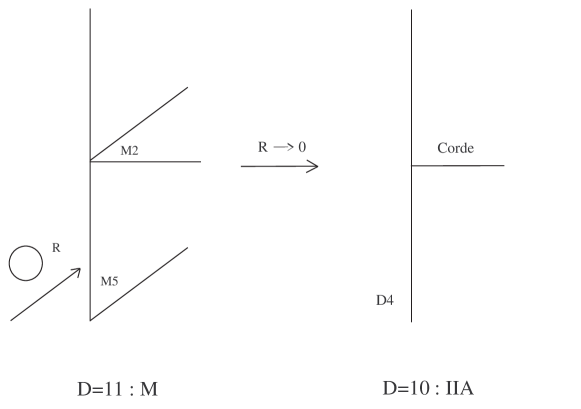
Figure 7.1: A M$5$ wrapped along a shrinked circle becomes a D4 brane.

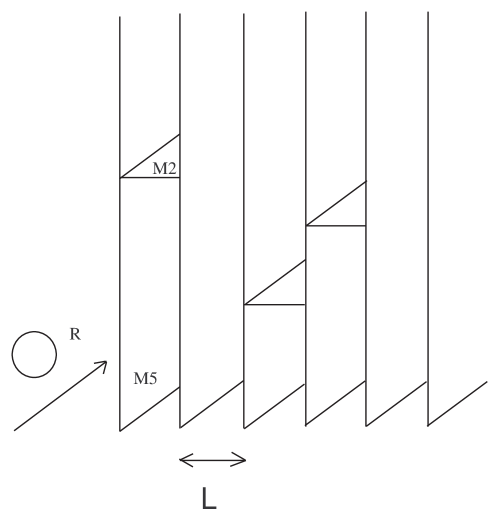
Figure 7.2: Parallel M$5$ separated by a distance of the order of $L$ with M$2$ stretching from one to the other.

Going back to the eleven dimensional picture, this observation suggests the existence of a non-Abelian extension of chiral two-forms living on the worldvolume of $n$ coinciding M$5$-branes worldvolumes, the theory of which is believed to be a non-trivial superconformally invariant quantum theory. The $5$-dimensional coupling arises as the radius of compactification $g^{2}_{YM}=R$.

M-theoretical considerations indicate that $n$ coinciding M5-branes constitute a highly unusual physical system. Indeed, the supergravity description of $n$ M5-branes predicts that both the entropy [148] and the two-point function for the stress-energy tensor [149] scale as $n^{3}$ in the large $n$ limit. Anomaly considerations lead to a similar behaviour [150]. Some people expect the interacting $(2,0)$ theory to fall outside the scope of perturbative covariant local field theory [94, 95, 96]. The same could be expected to occur for $SL(2,{\mathbb{Z}})$ duality symmetry of four dimensional non-Abelian vector theory, as is reviewed in subsection 7.1.3.

No-go theorem for self-dual fields

By free self-dual theories we understand a $2(p+1)$-dimensional linear $p$-brane electrodynamics described for

• $p$ even by two gauge fields dual to each other, as considered in the duality-symmetric formulation of subsection 4.1.1.

• $p$ odd by a single chiral gauge field, as discussed in subsection 4.1.3.

In some sense, self-dual gauge fields satisfy the more restrictive self-duality condition possible in their spacetime. We refer to the section 4.1 for a complete discussion of their self-duality equations.

Due to the following theorem, no local field theory seems to be able to describe a system of coinciding M5-branes.  

Theorem 3.

(No-go theorem for self-dual gauge fields) No consistent, local interactions of a set of free self-dual fields can deform the Abelian gauge transformations if the local deformed action (free action + interaction terms) continuously reduces to a sum of free, duality-symmetric, non-covariant actions in the zero limit for the coupling constant.  
The proof of this theorem is essentially algebraic [14, 15, 12] and is based on a cohomological reformulation of the Noether procedure for constructing consistent deformations [24]. The next section elaborates on the techniques required for the above proof.

Local deformations of the action cannot modify the Abelian nature of the algebra of the two-form gauge symmetries. The no-go theorem 3 holds under the assumption that the deformed action is continuous in the coupling constant (i.e., possible non-perturbative “miracles” are not investigated) and reduces, in the limit of vanishing coupling constant, to the action describing free chiral $2$-forms. In particular, no assumption is made on the polynomial order (cubic, quartic, …) of the interaction terms.

7.1.3 Compactification over a torus

New insights on EM-duality symmetry have been provided by M-theory. The type IIB string theory reduced on a circle is known to be T-dual to M-theory on a two-torus. Accordingly, the S-duality symmetry of the IIB string theory is a consequence of the invariance of the torus under large diffeomorphisms, the $SL(2,{\mathbb{Z}})$ symmetry of the IIB theory being associated with the modular group of the torus. Thus, in the M-theory context the S-duality of IIB string theory arises elegantly from simple geometric arguments. Likewise, the system of a single M5-brane system provides an appealing geometric understanding of EM-duality symmetry.

The worldvolume of the M$5$-brane supports a self-interacting chiral two-form potential which couples minimally to dyonic strings located at the intersection of the M$5$-brane and some M$2$-branes ending on it. If the M$5$-brane is wrapped around the torus, the T-dual picture in IIB theory is a D$3$-brane with fundamental strings ending on it. As a consequence the D$3$-brane itself is inert under the modular group $SL(2,{\mathbb{Z}})$. In terms of the D$3$-brane worldvolume theory, this symmetry translates into the EM-duality symmetry of Abelian BI theory [151, 152]. This sheds some light on the relation between duality-symmetric theories and chiral forms. Indeed, the e.o.m. (4.1.6) in four dimensions finds its origin in the self-duality equation of the three-form field strength living on the wrapped M5-brane. A ${\mathbb{Z}}_{4}$-duality transformation then corresponds to the “exchange” of the two circles in the compactification from M to IIB theory.

The next step of interest is to consider a system where $n$ wrapped M5-branes coincide. Unfortunately little is known about this interacting (2,0) superconformal theory. In the T-dual picture, the M5-branes appear as a set of coinciding D3-branes. Their dynamics is governed by a four-dimensional $U(n)$ supersymmetric DBI theory which, in the weak field limit, is an ordinary $U(n)$ non-Abelian gauge theory with ${\cal N}=4$ supersymmetry. The determination of all higher order terms in $\alpha^{\prime}$ is still an open question but some progress has been made recently in this direction (see [153, 154, 155, 156] and references therein). In any case, from the same arguments as before, the non-Abelian gauge theory on the coinciding D3-brane worldvolumes should possess an $SL(2,\mathbb{Z})$ symmetry.

The BRST techniques can be applied in a straightforward fashion to prove the results in [157] as well. There, deformations of chiral four-forms in ten dimensions were analyzed leading to the conclusion that the only consistent deformation in the type IIB coupling of the chiral four-form to the NS$\otimes$NS and the R$\otimes$R two-forms familiar from IIB supergravity.

No-go theorems for Yang-Mills fields

To conclude, let us consider the sourceless Yang-Mills equations and look after any duality symmetry property. They read

$$D_{A}\left(\begin{array}[]{c}F\\ $*$F\end{array}\right)=0,$$ (7.1.1)

where $A$ is Lie-algebra valued one-form, its curvature is equal to $F=D_{A}A=dA+A^{2}$ and the covariant derivative acts as $D_{A}=d+[A,\,]$ on other forms. Naively, one could think that the Yang-Mills equations (7.1.1) are left invariant by the duality rotation (2.1.12). However, that is not the case since the covariant derivative $D_{A}$ depends on $A$, which is not inert under the duality rotation.

In the seventies, two no-go theorems [86, 158] were found to prevent such a trivial generalization of EM-duality for Abelian gauge fields:

Proposition 7.1.

Generically, there is no infinitesimal transformation $\delta A$ which is able to implement the infinitesimal duality rotation

$$\delta F=*F\,\delta\alpha\,,\quad\delta*F=-F\,\delta\alpha.$$

Proposition 7.2.

There exists an example of gauge field $A$ with curvature $F=D_{A}A$ solution of the Yang-Mills equation $D_{A}*F=0$ but without “dual” gauge field $\tilde{A}$. In other words, there exists no vector field $\tilde{A}$ such that $*F=D_{\tilde{A}}\tilde{A}$.

The second no-go theorem is essentially a counterexample obtained by Gu and Yang [158]. It teaches us that the Poincaré lemma does not generalize straightforwardly to covariant derivative $D_{A}$ (Anyway, $D_{A}$ is not nilpotent since $D^{2}_{A}=[F,\,\,]$). This prevents a direct application of the scheme of the section 4.1 to obtain a duality-symmetric formulation of Yang-Mills theory.

Of course, no-go theorems have the weakness of their hypotheses. In consequence, a priori nothing prevents less “trivial” generalizations of EM-duality symmetry for non-Abelian gauge theories. The no-go theorem of the previous subsection further restricts the generalization possibilities [10]. Below, the proposition 7.6 gives a complete classification of the possible local interactions of a sum of duality-symmetric non-covariant actions.

7.1.4 $(4,0)$ superconformal theory

Hull considered the $5$-dimensional ${\cal N}=8$ (ungauged) supergravity, arising as a massless sector of M-theory compactified on a six-torus $T^{6}$. Using a line of arguments similar to those used previously, Hull conjectured that its strong coupling dual field theory should be a $6$-dimensional $(4,0)$ superconformal theory [94, 95, 96] containing an exotic fourth-rank tensor described in subsection 4.1.3. In [94], it was shown that the dimensional reduction of the free $6$-dimensional $(4,0)$ theory on a circle indeed gives the linearized $5$-dimensional ${\cal N}=8$ supergravity theory, with Planck length given by the circle radius $l_{P}=R$.

In the dimensional reduction, the $6$-dimensional self-dual gauge field in the irrep. of $GL(6,\mathbb{R})$ associated to the Young diagram reduces, in the $5$-dimensional picture, to gauge fields in irrep. of $GL(5,{\mathbb{R}})$ corresponding to the diagrams , , and . To show that, on-shell, these three gauge fields describe a single $5$-dimensional graviton it was necessary to dualize the $5$-dimensional gauge field to a symmetric tensor (see section 3.2 for more explanations).

No-go theorem for mixed symmetry type fields

Here also, we proved a no-go theorem which shows once again that dualization of non-Abelian gauge fields falls outside the conventional pattern. Indeed, the $5$-dimensional duality between a symmetric gauge field $h_{\mu\nu}$ and a mixed Young symmetry type gauge field $\tilde{h}_{\mu\nu\,|\,\rho}$ (see section 3.2) holds at the linearized level, but the following no-go theorem says that it seems difficult to reconstruct a self-interacting theory for $\tilde{h}_{\mu\nu\,|\,\rho}$ corresponding to the Einstein theory for the metric $g_{\mu\nu}=\eta_{\mu\nu}+h_{\mu\nu}$.

Theorem 4.

In $D\geq 5$ dimensions and under the hypothesis of • locality, • Lorentz invariance, • smooth deformation, there is no deformation of the free theory of the gauge field $M_{\mu\nu\,|\,\rho}\equiv\mbox{\footnotesize\begin{picture}(25.0,15.0)(0.0,0.0)\multiframe(0,6.5)(10.5,0){1}(10,10){$\mu$} \multiframe(0,-4)(10.5,0){1}(10,10){$\nu$} \multiframe(10.5,6.5)(10.5,0){1}(10,10){$\rho$} \end{picture}}$ which would modify the gauge algebra. If one adds the restriction that there should be • no deformation involving four derivatives or more in the Lagrangian, then there are no deformation of the free theory which would modify the gauge transformations without modifying the gauge algebra.  
Of course, one could add higher derivative terms involving product of the field strength and its derivatives. Such deformations modify neither the gauge algebra nor the gauge transformations.

7.2 Constructing deformations as a cohomological problem

This section follows closely [137, 159] and the section 2.2 of [160].

7.2.1 Noether method

Let $\stackrel{{\scriptstyle(0)}}{{S_{0}}}[\varphi^{i}]$ be a “free” action with “free” gauge symmetries

$$\delta_{\varepsilon}\varphi^{i}=\stackrel{{\scriptstyle\smash{(0)}}}{{R}}^{i}_{\alpha}\varepsilon^{\alpha}\,.$$ (7.2.1)

They lead to the so-called Noether identities [115] of the “free” theory

$${\delta\stackrel{{\scriptstyle(0)}}{{S}}\over\delta\varphi^{i}}\stackrel{{\scriptstyle\smash{(0)}}}{{R}}^{i}_{\alpha}=0\,.$$ (7.2.2)

We now start to perturb the “free” theory by introducing new terms $\stackrel{{\scriptstyle(i)}}{{S_{0}}}$ ($i=1,2,\ldots$) to the action. The perturbation is controlled by a coupling constant $g$ which appears in the expansion of the “deformation” $S_{0}$,

$$S_{0}=\stackrel{{\scriptstyle(0)}}{{S_{0}}}+g\stackrel{{\scriptstyle(1)}}{{S_{0}}}+g^{2}\stackrel{{\scriptstyle(2)}}{{S_{0}}}+...$$ (7.2.3)

By consistent deformations, one means that the deformed action should be gauge invariant under the (possibly deformed) gauge transformation rules,

$$R^{i}_{\alpha}=\stackrel{{\scriptstyle\smash{(0)}}}{{R}}^{i}_{\alpha}+g\stackrel{{\scriptstyle\smash{(1)}}}{{R}}^{i}_{\alpha}+g^{2}\stackrel{{\scriptstyle\smash{(2)}}}{{R}}^{i}_{\alpha}+....$$ (7.2.4)

As in the “free” case, it may be translated into the requirement that the Noether identities should hold to all orders

$${\delta{S}\over\delta\varphi^{i}}{R}^{i}_{\alpha}=0,$$ (7.2.5)

where,

$$\delta_{\varepsilon}\varphi^{i}=R^{i}_{\alpha}\varepsilon^{\alpha}.$$ (7.2.6)

As one can see by expanding (7.2.5) order by order in the coupling constant, there are a priori an infinite number of consistency conditions (of increasing complexity) to take into account.

For reducible theories, which is the case relevant to chiral $p$-forms, there are even additional constraints. The gauge transformations of the free theory are not independent,

$$\stackrel{{\scriptstyle\smash{(0)}}}{{R}}^{i}_{\alpha}\stackrel{{\scriptstyle\smash{(0)}}}{{Z}}^{\alpha}_{A}=0$$ (7.2.7)

(possibly on-shell). There could be higher reducibility conditions (e.g. reducibilities of reducibilities). One must then also impose that the gauge transformations remain reducible, possibly in a deformed way. This yields further constraints. The conclusion is that to be consistent, the deformation should preserve the gauge structure of the theory.

7.2.2 BRST formulation

A convenient toolkit for translating the problem of consistent interactions into a cohomological problem is the antifield formalism [113]. If the undeformed theory is actually free, it is a relatively easy task to solve the master equation for the “free” theory. Let $\stackrel{{\scriptstyle(0)}}{{S}}$ be a solution of the undeformed master equation $(\stackrel{{\scriptstyle(0)}}{{S}},\stackrel{{\scriptstyle(0)}}{{S}})=0$. Since the master equation captures all the information about the gauge structure of the theory, the existence of a consistent deformation $S_{0}$ of the original gauge invariant action $\stackrel{{\scriptstyle(0)}}{{S}}_{0}$ is equivalent to the existence of a deformation $S$ of $\stackrel{{\scriptstyle(0)}}{{S}}$,

$$S=\stackrel{{\scriptstyle(0)}}{{S}}+g\stackrel{{\scriptstyle(1)}}{{S}}+g^{2}\stackrel{{\scriptstyle(2)}}{{S}}+...$$ (7.2.8)

which is a solution to the master equation $(S,S)=0$. Expanding this equation order by order in the coupling constant yields various consistency relations,

$$(\stackrel{{\scriptstyle(0)}}{{S}},\stackrel{{\scriptstyle(0)}}{{S}}) =0$$ (7.2.9)

$$(\stackrel{{\scriptstyle(0)}}{{S}},\stackrel{{\scriptstyle(1)}}{{S}}) =0$$ (7.2.10)

$$2(\stackrel{{\scriptstyle(0)}}{{S}},\stackrel{{\scriptstyle(2)}}{{S}})+(\stackrel{{\scriptstyle(1)}}{{S}},\stackrel{{\scriptstyle(1)}}{{S}}) =0$$

$$\vdots\ \ \ .$$

The first equation is satisfied by assumption. Now comes the cohomology. Let $\stackrel{{\scriptstyle(0)}}{{s}}$ be the “free” BRST differential defined by

$$\stackrel{{\scriptstyle(0)}}{{s}}\equiv(\stackrel{{\scriptstyle(0)}}{{S}},\cdot)$$ (7.2.12)

The crucial point for us is now that the second equation states that $\stackrel{{\scriptstyle(1)}}{{S}}$ is a cocycle for $\stackrel{{\scriptstyle(0)}}{{s}}$. Furthermore, if $\stackrel{{\scriptstyle(1)}}{{S}}$ were a coboundary, $\stackrel{{\scriptstyle(1)}}{{S}}=(\stackrel{{\scriptstyle(1)}}{{T}},\stackrel{{\scriptstyle(0)}}{{S}})$, we can show that this would correspond to a trivial deformation of $\stackrel{{\scriptstyle(0)}}{{S}}$ (i.e. a deformation which amounts to a simple redefinition of the fields). The solution of the master equation $S_{0}$ is of definite vanishing ghost number, therefore the cohomology group of interest in the study of first order deformations is $H^{0}(\stackrel{{\scriptstyle(0)}}{{s}})$.

For practical purpose, we more precisely consider deformations which are local in spacetime, i.e., we impose that $\stackrel{{\scriptstyle(1)}}{{S}},\stackrel{{\scriptstyle(2)}}{{S}},...$ be local functionals. Reformulating the equations in terms of the Lagrange densities takes care of this problem. Then, in the local context, the proper cohomology group to evaluate is $H^{0,D}(\stackrel{{\scriptstyle(0)}}{{s}}\mid d)$ where the first and second superscripts denote the ghost number and form degree, respectively.

Let us consider briefly the case when all the representatives of $H^{D,0}(\stackrel{{\scriptstyle(0)}}{{s}}\mid d)$ can be taken not to depend on the antifields, which is the situation met for the systems considered in this chapter. We may take the first-order deformations $\stackrel{{\scriptstyle(1)}}{{\cal{S}}}$ to be antifield-independent. In this case equation (7.2.10) reduces to $(\stackrel{{\scriptstyle(0)}}{{S}},\stackrel{{\scriptstyle(2)}}{{S}})=0$ and implies that the deformation at order $g^{2}$ defines also an element of $H^{D,0}(\stackrel{{\scriptstyle(0)}}{{s}}\mid d)$. We can thus take $\stackrel{{\scriptstyle(2)}}{{S}}$ not to depend on the antifields either. Proceeding in this manner order by order in the coupling constant, we conclude that the additional terms in $S$ are all independent of the antifields. Since the antifield-dependent terms in the deformation of the master equation are related to the deformations of the gauge transformations, this means that there is no deformation of the gauge transformations. Summarizing, if there is no non-trivial dependence on the antifields in $H^{D,0}(\stackrel{{\scriptstyle(0)}}{{s}}\mid d)=0$, the only possible consistent interactions are of the first class and do not modify the gauge symmetry.

7.3 Local BRST cohomology

We will illustrate the computation of the local BRST cohomology in vanishing ghost number on a particular example: a system of N free chiral 2-forms $A^{A}_{ij}$ ($A=1,\ldots,N$), the dynamics of which is described by the non-covariant action [161, 98],

$$S_{0}[A^{A}_{ij}]=\sum_{A}\int dt\,d^{5}x\,B^{A\,ij}(\dot{A}^{A}_{ij}-B^{A}_{ij}),\quad(A=1,\ldots,N),$$ (7.3.1)

where

$$B^{A\,ij}=\frac{1}{6}\epsilon^{ijklm}F^{A}_{klm}=\frac{1}{2}\epsilon^{ijklm}\partial_{k}A^{A}_{lm}.$$ (7.3.2)

The action (7.3.1) differs from the one in [39, 145] where a space-like dimension was singled out. Here we take time as the distinguished direction; from the point of view of the PST formulation [146, 147], the two approaches simply differ in the gauge fixation.

We work in Minkowski spacetime. This implies, in particular, that the topology of the spatial sections are the same as ${\mathbb{R}}^{5}$. Most of our considerations would go unchanged in a curved background of the product form ${\mathbb{R}}\times\Sigma$ provided the De Rham cohomology groups $H^{2}(\Sigma)$ and $H^{1}(\Sigma)$ of the spatial sections $\Sigma$ vanish. [If $H^{2}(\Sigma)$ is non-trivial, there are additional gauge symmetries besides (7.3.3) below, given by time-dependent spatially closed $2$-forms; similarly, if $H^{1}(\Sigma)$ is non-trivial, there are additional reducibility identities besides (7.3.4) below. We would thus need additional ghosts and ghosts of ghosts. These, however, would not change the discussion of local Lagrangians because they would be global in space (and local in $t$).]

The action $S_{0}$ is invariant under the following gauge transformations

$$\delta_{\Lambda}A^{A}_{ij}=\partial_{i}\Lambda^{A}_{j}-\partial_{j}\Lambda^{A}_{i},$$ (7.3.3)

because $B^{A\,ij}$ is gauge-invariant and identically transverse ($\partial_{i}B^{A\,ij}\equiv 0$) . As $\delta A_{ij}^{A}=0$ for

$$\Lambda_{i}^{A}=\partial_{i}\varepsilon^{A},$$ (7.3.4)

this set of gauge transformations is reducible. This exhausts completely the redundancy in $\Lambda_{i}^{A}$ since $H^{1}({\mathbb{R}}^{5})=0$.

The equations of motion obtained from $S_{0}[A^{A}_{ij}]$ by varying $A^{A}_{ij}$ are

$$\epsilon^{ijklm}\partial_{k}\dot{A}^{A}_{lm}-2\partial_{k}F^{A\,ijk}=0\Leftrightarrow\epsilon^{ijklm}\partial_{k}(\dot{A}^{A}_{lm}-B^{A}_{lm})=0.$$ (7.3.5)

Using $H^{2}({\mathbb{R}}^{5})=0$, one finds that the general solution of (7.3.5) is

$$\dot{A^{A}_{ij}}-B^{A}_{ij}=\partial_{i}\Lambda^{A}_{j}-\partial_{j}\Lambda^{A}_{i}.$$ (7.3.6)

The ambiguity in the solutions of the equations of motion is thus completely accounted for by the gauge freedom (7.3.3). Hence the set of gauge transformations is complete.

We can view $\Lambda^{A}_{i}$ as $A^{A}_{0i}$, so the equation (7.3.6) can be read as the self-duality equation

$$F^{A}_{0ij}-*F^{A}_{0ij}=0,$$ (7.3.7)

where $F^{A}_{0ij}=\dot{A^{A}_{ij}}+\partial_{i}A^{A}_{j0}+\partial_{j}A^{A}_{0i}$. Alternatively, one may use the gauge freedom to set $\Lambda^{A}_{i}=0$, which yields the self-duality condition in the temporal gauge.

7.3.1 Fields - Antifields - Solution of the master equation

The solution of the master equation is easy to construct in this case because the gauge transformations are Abelian.

The fields in presence here are

$$\{\Phi^{M}\}=\{A^{A}_{ij},C^{A}_{i},\eta^{A}\}.$$ (7.3.8)

The ghosts $C^{A}_{i}$ correspond to the gauge parameters $\Lambda^{A}_{i}$, and the ghosts of ghosts $\eta^{A}$ correspond to $\epsilon^{A}$.

Now, to each field $\Phi^{M}$ we associate an antifield $\Phi^{*}_{M}$. The set of antifields is then

$$\{\Phi^{*}_{M}\}=\{A^{*Aij},C^{*Ai},\eta^{*A}\}.$$ (7.3.9)

The fields and antifields have the respective parities

$$\epsilon(A^{A}_{ij})=\epsilon(\eta^{A})=\epsilon(C^{*Ai})=0$$ (7.3.10)

$$\epsilon(C^{A}_{i})=\epsilon(A^{*Aij})=\epsilon(\eta^{*A})=1.$$ (7.3.11)

The antibracket is defined as

$$(X,Y)=\int d^{n}x\left(\frac{\delta^{R}X}{\delta\Phi^{M}(x)}\frac{\delta^{L}Y}{\delta\Phi^{*}_{M}(x)}-\frac{\delta^{R}X}{\delta\Phi^{*}_{M}(x)}\frac{\delta^{L}Y}{\delta\Phi^{M}(x)}\right)$$ (7.3.12)

where $\delta^{R}/\delta Z(x)$ and $\delta^{L}/\delta Z(x)$ denote functional right- and left-derivatives.

Because the set of gauge transformations is complete and defines a closed algebra, the (minimal, proper) solution of the master equation $(S,S)=0$ takes the general form

$$S=S_{0}+\sum_{M}\int(-)^{{\epsilon}(M)}\Phi^{*}_{M}s\Phi^{M},$$ (7.3.13)

where ${{\epsilon}(M)}$ is the Grassmann parity of $\Phi^{M}$. More explicitly, we have

$$S=S_{0}+\sum_{A}\int dtd^{5}x(A^{*Aij}\partial_{i}C^{A}_{j}-C^{*Ai}\partial_{i}\eta^{A})$$ (7.3.14)

The solution $S$ of the master equation captures all the information about the gauge structure of the theory : the Noether identities, the closure of the gauge transformations algebra and the higher order gauge identities are contained in the master equation. The existence of $S$ reflects the consistency of the gauge transformations.

7.3.2 BRST operator

The BRST operator $s$ is obtained by taking the antibracket with the proper solution $S$ of the classical master equation,

$$s\,X=(S,X).$$ (7.3.1)

The BRST operator can be decomposed as

$$s=\delta+\gamma$$ (7.3.2)

where $\delta$ is the Koszul–Tate differential [115]. What distinguishes $\delta$ and $\gamma$ is the antighost number ($antigh$) defined through

$$antigh(A^{A}_{ij})=antigh(C^{A}_{i})=antigh(\eta^{A})=0,$$ (7.3.3)

$$antigh(A^{*A\,ij})=1,\quad antigh(C^{*A\,i})=2,\quad antigh(\eta^{*A})=3.$$ (7.3.4)

The ghost number ($gh$) is related to the antighost number by

$$gh=puregh-antigh$$ (7.3.5)

where $puregh$ is defined through

$$puregh(A^{A}_{ij})=0,\quad puregh(C^{A}_{i})=1,\quad puregh(\eta^{A})=2,$$ (7.3.6)

$$puregh(A^{*A\,ij})=puregh(C^{*A\,i})=puregh(\eta^{*A})=0.$$ (7.3.7)

The differential $\delta$ is characterized by $antigh(\delta)=-1$, i.e. it lowers the antighost number by one unit and acts on the fields and antifields according to

$$\delta A^{A}_{ij} = \delta C^{A}_{i}=\delta\eta^{A}=0,$$ (7.3.8)

$$\delta A^{*A\,ij} = 2\partial_{k}F^{A\,kij}-\epsilon^{ijklm}\partial_{k}\dot{A}^{A}_{lm},$$ (7.3.9)

$$\delta C^{*A\,i} = \partial_{j}A^{*A\,ij},$$ (7.3.10)

$$\delta\eta^{*A} = \partial_{i}C^{*A\,i}.$$ (7.3.11)

The differential $\gamma$ is characterized by $antigh(\gamma)=0$ and acts as

$$\gamma A^{A}_{ij} = \partial_{i}C^{A}_{j}-\partial_{j}C^{A}_{i},$$ (7.3.12)

$$\gamma C^{A}_{i} = \partial_{i}\eta^{A},$$ (7.3.13)

$$\gamma\eta^{A} = 0,$$ (7.3.14)

$$\gamma A^{*A\,ij} = \gamma C^{*A\,i}=\gamma\eta^{*A}=0.$$ (7.3.15)

Furthermore we have,

$$sx^{\mu}=0,\;s(dx^{\mu})=0.$$ (7.3.16)

7.3.3 Local forms - Algebraic Poincaré lemma

A local function is a function of the fields, the ghosts, the antifields, and their derivatives up to some finite order $k$ (which depends on the function),

$$f=f(\Phi,\partial_{\mu}\Phi,\ldots,\partial_{\mu_{1}}\ldots\partial_{\mu_{k}}\Phi).$$ (7.3.17)

A local function is thus a function over a finite dimensional vector space $J^{k}$ called jet space. A local form is an exterior polynomial in the $dx^{\mu}$’s with local functions as coefficients. The algebra of local forms will be denoted by ${\cal{A}}$. In practice, the local forms are polynomial in the ghosts and the antifields, as well as in the differentiated fields, so we shall from now on assume that the local forms under consideration are of this type. We can actually show that polynomiality in the ghosts, the antifields and their derivatives follows from polynomiality in the derivatives of the $A_{ij}$ by an argument similar to the one used in [162] for $1$-forms; and polynomiality in the derivatives is automatic in our perturbative approach where we work order by order in the coupling constant(s).

Note that we also exclude an explicit $x$-dependence of the local forms. We could allow for one without change in the conclusions. In fact, as we shall indicate below, allowing for an explicit $x$-dependence simplifies some of the proofs. We choose not to do so here since the interaction terms in the Lagrangian should not depend explicitly on the coordinates in the Poincaré-invariant context.

The following proposition describes the cohomology of $d$ in the algebra $\cal A$ of local forms, in degree $q<D$.

Proposition 7.3.

The cohomology of $d$ in the algebra of local forms of degree $q<D$ is given by

$$H^{0}(d,{\cal A}) \cong {\mathbb{R}},$$

$$H^{q}(d,{\cal A}) = \{\hbox{Constant Forms}\},\;0<q<D.$$

Constant forms are by definition polynomials in the $dx^{\mu}$’s with constant coefficients. This proposition is called the algebraic Poincaré lemma (for $q<D$). There exist many proofs of this lemma in the literature.

Constant $q$-forms are trivial in degree $0<q<D$ in the algebra of local forms with an explicit $x$-dependence; e.g., $dx^{0}=df$, where $f$ is the $x^{0}$-dependent function $f=x^{0}$. Thus, in this enlarged algebra, the cohomology of $d$ is simpler and vanishes in degrees $0<q<D$. This is the reason why the calculations are somewhat simpler when we allow for an explicit $x$-dependence.

We work in a formalism where the time direction is privileged. For this reason, it is useful to introduce the following notation : the $l$-th time derivative of a field $\Phi$ (including the ghosts and antifields) is denoted by $\Phi^{(l)}$ ($=\partial_{0}^{l}\Phi$), and the spatial differential is denoted by $\tilde{d}=dx^{i}\partial_{i}$.

A local spatial form is an exterior polynomial in the spatial $dx^{k}$’s with coefficients that are local functions. The algebra of local spatial forms will be denoted by $\widetilde{\cal{A}}$. If we write the set of the generators of the jet space $J^{k}$ as

$$\{\Phi^{(l_{0})},\partial_{i_{1}}\Phi^{(l_{1})},\ldots,\partial_{i_{1}}\dots\partial_{i_{k}}\Phi^{(0)};\,\,l_{j}=0,\ldots,k-j\},$$ (7.3.18)

it is clear that

Proposition 7.4.

The cohomology of $\tilde{d}$ in the algebra $\widetilde{\cal{A}}$ of local spatial forms of degree $q<D-1$ is given by

$$H^{0}(\tilde{d},\widetilde{\cal{A}}) \cong {\mathbb{R}},$$

$$H^{q}(\tilde{d},\widetilde{\cal{A}}) = \{\hbox{Constant spatial forms}\},\;0<q<D-1.$$

A similar decomposition of space and time derivatives occurs of course in the Hamiltonian formalism. A discussion of the problem of consistent deformations of a gauge invariant action has been carried out in the Hamiltonian context in [163, 164].

7.3.4 Wess-Zumino consistency condition

The local BRST cohomology is defined as the cohomology $H(s\mid d,{\cal A})$ of $s$ modulo $d$ in the graded algebra $\cal A$ of local forms. The algebra $\cal A$ is graded according to many degrees ; for instance, the form degree, the pure ghost number, the antighost number, the degree of polynomiality, etc. Two degrees are of particular interest: the form degree $p$ and the ghost number $g$. This grading of ${\cal A}=\oplus_{p,g}{\cal A}^{p,g}$ induces a grading of the local BRST cohomology

$$H(s\mid d,{\cal A})\equiv\oplus_{p,g}\,H^{p,g}(s\mid d)$$ (7.3.19)

where $H^{p,g}(s\mid d)$ is defined by (i) the so-called Wess-Zumino consistency condition, that is $\alpha^{p,g}\in H^{p,g}(s\mid d)$ if and only if

$$s\alpha^{p,g}+d\beta^{p-1,g+1}=0\,,\quad\alpha^{p,g}\in{\cal A}^{p,g}\,,\,\,\alpha^{p-1,g+1}\in{\cal A}^{p-1,g+1}\,,$$ (7.3.20)

and (ii) the equivalence relation

$$\alpha^{p,g}\sim\alpha^{p,g}+s\rho^{p,g-1}+d\sigma^{p-1,g}\,,\quad\rho^{p,g-1}\in{\cal A}^{p,g-1}\,,,\,\,\sigma^{p-1,g}\in{\cal A}^{p-1,g}\,.$$ (7.3.21)

Now, all the necessary tools have been presented to proof the theorem 3. As explained in subsection 7.2.2, it follows from the

Proposition 7.5.

There is no non trivial dependence on the antifields for the elements of $H^{D,0}(s\mid d)$.

In conclusion the proof of theorem 3 reduces to the computation of the cohomology $H^{D,0}(s\mid d)$ for the free theory. The detailed computation for the chiral two-forms system, using homological perturbation theory techniques, has been placed in the appendix G since the proof is rather lengthy and technical. It follows the path cleared by the general theorems of [165, 162].

7.4 Self-interactions of a single gauge vector

In this section we want to generalize the PST action describing a single free Maxwell field to an interacting theory with only one on-shell gauge vector (the e.o.m. allows to express on of the two gauge field in term of the other). The interacting model should of course maintain the Lorentz covariance and should lead to a deformed self-duality condition. Firstly, we review in subsec. 7.4.1 how this has been achieved in the non-covariant approach, then we extend it in subsec. 7.4.2 for the covariant case, and finally we look for the solutions of the Courant-Hilbert equation.

7.4.1 The return of the Courant-Hilbert equation

We want to introduce self-couplings for the non-covariant EM duality-symmetric action. In [41] it was proposed to attack this problem using the Hamiltonian formulation, which is appropriate for first-order actions. Let us review their approach, trying to justify completely the ansatz in the light of the results obtained in the appendix G, where a classification of local consistent deformations is given for a set of chiral two-forms. The analogue of proposition G.1 for the four-dimensional duality-symmetric theory under consideration is the

Proposition 7.6.

All consistent, continuous, local deformations of a system of free Abelian vector fields (labelled by indices $A,B=1,\cdots,N$) described by a sum of $N$ free, duality-symmetric, non-covariant actions as the coupling constant goes to zero, are only of two types:

• Those which are strictly invariant under the original gauge transformations $A_{i}^{\alpha\,A}\rightarrow A_{i}^{\alpha\,A}+\partial_{i}\Lambda^{\alpha\,A}$; they are polynomials in the gauge-invariant fieldstrength $F^{\alpha A}_{ij}=\partial_{i}A_{j}^{\alpha\,A}-\partial_{j}A_{i}^{a\,A}$ and their partial derivatives, i.e. they are of the form

  $$\int d^{4}x\,f(\partial_{\mu_{1}\dots\mu_{r}}F^{\alpha\,A}_{ij})\,,\quad(r=0,1,\ldots)\,.$$ (7.4.1)

• Those which are invariant only up to a boundary term; they are linear combinations of Chern-Simons like terms, i.e.

  $$\int d^{4}x\,\lambda_{rs\,\alpha\beta\,AB}\,(\partial_{0})^{r}A_{i}^{\alpha\,A}(\partial_{0})^{s}B^{\beta\,B\,i}\,,$$ (7.4.2)

  where $\lambda_{rs\,\alpha\beta\,AB}$ ($\alpha,\beta=1,2$) are constants such that $\lambda_{sr\,\beta\alpha\,BA}=\lambda_{rs\,\alpha\beta\,AB}\,$.

For instance, the Hamiltonian of the free theory is a term of type I, as well as the Hamiltonian for Born-Infeld theory. The kinetic term is of type II.

From the very beginning we state three basic requirements made on the model in this approach: (i) The deformation remains a first-order action, (ii) manifest rotation invariance, (iii) manifest duality-symmetry. The first assumption comes from the fact that we work in Hamiltonian formalism. The second and third requirements simply extend the properties of the free model.

The requirement (i) combined with proposition 7.6 and with the fact that we deal with a single on-shell vector gauge field ($N=1$) eliminates deformations of the type $II$ besides the one without any derivative. Thus, the non-linear action is

$$S=-{1\over 2}\int d^{4}x\,B^{i\alpha}J_{\alpha\beta}E^{\beta}_{i}-\int dx^{0}H,$$ (7.4.3)

where

$$H=\int d^{3}x\left({\mathcal{H}}(\partial_{i_{1}\dots i_{k-1}}B^{\alpha}_{i_{k}})+\chi A_{i}^{\alpha}B^{i\alpha}\right)$$ (7.4.4)

stands for the Hamiltonian of the model. The constant factor of the Chern-Simons like term is denoted by $\chi$. If we now restrict ourself to (iv) Hamiltonian densities that do not explicitly depend on the derivatives of the magnetic field: ${\mathcal{H}}={\mathcal{H}}(B^{\alpha A}_{i})$, we can deduce from (ii) and (iii) that the Hamiltonian density ${\mathcal{H}}$ only depends on two independent space scalars that are manifestly duality invariant, namely

$$y_{1}=\frac{1}{2}B^{\alpha}_{i}B^{\alpha i}\,,\;\;y_{2}=\frac{1}{4}B^{\alpha}_{i}B^{\beta i}B^{\alpha}_{j}B^{\beta j}\,.$$ (7.4.5)

We set ${\mathcal{H}}=f(y_{1},y_{2})$.

Now, all the symmetries are manifest except Lorentz symmetry. With the help of tensor calculus, it is rather easy to construct interactions that preserve Lorentz invariance. But there is an alternative way to control Lorentz invariance. It is through the commutation relations of the energy-momentum tensor components: Dirac and Schwinger have established a sufficient condition for a manifestly rotation and translation invariant theory (in space) to be also Lorentz-invariant [119, 120]. The condition becomes also necessary when one turns to couplings with gravitation [120] or if one asks for diffeomorphism-invariance (“path independence of the dynamical evolution”) [166]. The Dirac-Schwinger criterion yields in our case $\chi=0$ and a non-linear first-order differential equation for $f$ [42]

$$f_{1}^{2}+2y_{1}f_{1}f_{2}+2(y_{1}^{2}-y_{2})f_{2}^{2}=1\,,$$ (7.4.6)

where $f_{i}=\frac{\partial f}{\partial y_{i}}$ for $i=1,2.$ The equation (7.4.6) can be given a simpler look by the change of variables

$$\left\{\begin{array}[]{lll}y_{1}&=&u_{+}+u_{-}\\ y_{2}&=&u^{2}_{+}+u^{2}_{-}\end{array}\right.\,.$$ (7.4.9)

Denoting the function derivatives by $f_{\pm}\equiv{\partial f\over\partial u_{\pm}}$, one gets again the Courant-Hilbert equation (2.5.26). It is not surprising to find the same equation for the Hamiltonian density and the Lagrangian density because they are related by a Legendre transformation, and Legendre transformation relates a model and its dual [37].

This rederivation of (2.5.26) proves that the class of duality-symmetric non-linear electrodynamics considered in subsection 2.5.5 covered the most general set of physically natural possibilities, since the Dirac-Schwinger condition becomes necessary when one turns to general covariance. Combining the proposition 7.6 with the Dirac-Schwinger criterion, we prove the stronger

Corollary 7.1.

Any

• non-trivial

• local

• consistent

• diffeomorphism-invariant

• analytic in the weakly-coupled regime

deformation of the four-dimensional free non-(manifestly)-covariant self-dual gauge field theory is entirely characterized by a function $\Psi(t)$ satisfying the conditions $(i)-(iv)$ of theorem 1.

Therefore, the class satisfying the reasonable physical requirements of the corollary 7.1 is precisely the class infinite class of duality-symmetric theories of the corollary 2.1. Once again, we observe that manifest duality symmetry does not easily combine with Lorentz symmetry and locality.

7.4.2 Self-couplings of the PST model

In this section, we “covariantize” the results of the previous section, generalizing the procedure of the free PST model. In this way, we construct a deformed theory describing self-couplings of one Maxwell field (on-shell) which is manifestly duality-symmetric and Lorentz covariant.

Just as in the case of the free system the covariantization involves an auxiliary field and an extra gauge invariance. As we showed in [10], it is the deformation of this symmetry that leads to the Courant-Hilbert equation.

To recall the assumptions we stress that it seems natural to require the interacting action to satisfy the same kind of symmetries as the free one. In other words we should expect besides the Lorentz invariance also a manifest duality-symmetry. From the analysis on the consistent deformations of the non-covariant action, we know that the interaction should depend only on the field strengths and its derivatives. If we are in the weakly varying field limit, this reduces the number of independent invariants to only two (since we neglect derivative of the field strength), namely

$$z_{1}=\frac{1}{2}\tilde{\mathcal{H}}^{\alpha}_{\mu}\tilde{\mathcal{H}}^{\alpha\,\mu}\,,\;\;z_{2}=\frac{1}{4}\tilde{\mathcal{H}}^{\alpha}_{\mu}\tilde{\mathcal{H}}^{\beta\,\mu}\tilde{\mathcal{H}}^{\alpha}_{\nu}\tilde{\mathcal{H}}^{\beta\,\nu}\,.$$ (7.4.10)

Similarly to the non-covariant situation, we keep the “kinetic” term and add an interaction term $f(z_{1},z_{2})$ depending only on the invariants of the theory. As an assumption, we take the following action for a self-interacting gauge vector

$$S^{I} = \int d^{4}x\,\left(\frac{1}{2}{\mathcal{H}}^{\alpha}_{\mu}\tilde{\mathcal{H}}^{\alpha\,\mu}-f(z_{1},z_{2})\right)\,$$ (7.4.11)

A priori $f$ is a general function but the connection with the free theory (5.3.1) imposes its analyticity at the origin and its reduction to $f\rightarrow z_{1}$ in the weak field limit. We are going to restrict the class of possible interactions by demanding the field equations as well as the action to remain invariant (up to a boudary term) under some modified transformations of type (5.3.7)-(5.3.9). In fact we deform only the gauge symmetry (5.3.8) to

$$\delta A_{\mu}^{\alpha}=\epsilon^{\beta\alpha}({\mathcal{H}}_{\mu}^{\beta}-{\cal K}_{\mu}^{\beta})\frac{\phi}{\sqrt{-u^{2}}}\,, \,\delta a=\phi\,,$$ (7.4.12)

where we denoted the deforming contribution as ${\cal K}_{\mu}^{\beta}=\frac{\delta f}{\delta\tilde{\mathcal{H}}^{\beta\,\mu}}\,.$ In the free limit case the last transformation is nothing but (5.3.8), as it should be.

Using an approach similar to the free case (i.e. gauge-fixing (5.3.9) the solution to the equations of motion determined by $S^{I}$ read

$${\mathcal{H}}^{\alpha}_{\mu}={\cal K}^{\alpha}_{\mu}=f_{1}\tilde{\mathcal{H}}^{\alpha}_{\mu}+f_{2}(\tilde{\mathcal{H}}^{3})_{\mu}^{\alpha}\,,$$ (7.4.13)

where $f_{i}=\frac{\partial f}{\partial z_{i}}$ for $i=1,2$ and $(\tilde{\mathcal{H}}^{3})_{\mu}^{\alpha}=\tilde{\mathcal{H}}^{\beta}_{\mu}\tilde{\mathcal{H}}^{\beta\,\nu}\tilde{\mathcal{H}}^{\alpha}_{\nu}$. The general variation of this equation is very intricate but we can make use of the other symmetries of the system (Lorentz and SO(2) rotation invariance) to choose a basis in which the vector $u_{\mu}=\delta_{\mu}^{0}$ (i.e. it is time-like) and the only non-vanishing components of the tensor $\tilde{\mathcal{H}}^{\alpha}_{\mu}$ are

$$\tilde{\mathcal{H}}^{1}_{1}=\lambda_{+}\,,\quad\quad\tilde{\mathcal{H}}^{2}_{2}=\lambda_{-}\,.$$ (7.4.14)

In this special choice the equation of motion reduces to only

$$\gamma_{\pm}=\lambda_{\pm}(f_{1}+f_{2}\lambda_{\pm}^{2})$$ (7.4.15)

where $\gamma_{+}={\mathcal{H}}^{1}_{1}$, $\gamma_{-}={\mathcal{H}}^{2}_{2}$ are the non-zero components of ${\mathcal{H}}^{\alpha}_{\mu}$ in this basis. After using the field equations (7.4.13), the variation (7.4.13) takes the form

$$\delta{\mathcal{H}}^{1}_{3}=\lambda_{-},\quad\delta\tilde{\mathcal{H}}^{1}_{3}=\gamma_{-}.$$ (7.4.16)

The variation of the e.o.m. (7.4.15) is then

$$\lambda_{-}=f_{1}\gamma_{-}+f_{2}\gamma_{-}\lambda_{+}^{2}\,,$$

which upon using once more the equations of motion gives

$$(f_{1}+f_{2}\lambda^{2}_{+})(f_{1}+f_{2}\lambda^{2}_{-})=1\,.$$ (7.4.17)

We can reformulate it in terms of the two invariants $z_{1}=\frac{1}{2}(\lambda^{2}_{+}+\lambda^{2}_{-})$ and $z_{2}=\frac{1}{4}(\lambda^{4}_{+}+\lambda^{4}_{-})$. Eventually performing the transformation (7.4.9) we end up with the Courant-Hilbert equation (2.5.26). Thus, we derived this equation by imposing the invariance of the equations of motion under the gauge transformation (7.4.12).

We now briefly show that the action is also invariant (up to total derivatives) under the same gauge transformations (7.4.12). Inserting (7.4.12) in the general variation of the action

$$\delta S^{I} = \int d^{4}x\,\left[({\mathcal{H}}^{\alpha}_{\mu}-{\cal K}^{\alpha}_{\mu})\delta_{A,a}\tilde{\mathcal{H}}^{\alpha\,\mu}+\frac{1}{2}\delta_{a}{\mathcal{H}}^{\alpha}_{\mu}\tilde{\mathcal{H}}^{\alpha\,\mu}-\frac{1}{2}{\mathcal{H}}^{\alpha}_{\mu}\delta_{a}\tilde{\mathcal{H}}^{\alpha\,\mu}\right]$$

and, after canceling the contributions of first-order in the derivatives of $f$ coming from the variation with respect to $A_{\mu}^{\alpha}$, respectively $a$, we deduce

$$\delta S^{I} = \frac{1}{2}\int d^{4}x\,\epsilon^{\mu\nu\lambda\rho}\epsilon^{\beta\alpha}\delta v_{\mu}v_{\nu}\left(\tilde{\mathcal{H}}^{\alpha}_{\lambda}\tilde{\mathcal{H}}^{\beta}_{\rho}-{\cal K}^{\alpha}_{\lambda}{\cal K}^{\beta}_{\rho}\right)\,.$$

We evaluate this variation in the special basis mentioned above and get

$$\delta S^{I}=-2\int d^{4}x\,\delta v_{3}\,\lambda_{+}\lambda_{-}\,[(f_{1}+f_{2}\lambda^{2}_{+})(f_{1}+f_{2}\lambda^{2}_{-})-1]\,.$$ (7.4.18)

The restriction (7.4.17) is sufficient to guarantee the invariance of both, field equations and action, since upon applying the Courant-Hilbert equation (2.5.26) we get $\delta S^{I}=0$.

To conclude, we have constructed a modified Lorentz covariant theory that also possesses a manifest EM duality. The allowed self-interactions are restricted to a class of functions of two variables that must satisfy the Courant-Hilbert equation. Our analysis straightforwardly generalizes the PST formulation of BI electrodynamics [147] to any non-linear theory of a single gauge vector in four dimensions.

Appendix A Algebraic preliminaries

A.1 Fundamental structures

A ring $\Lambda$ is a set endowed with two internal laws $+$ and $\cdot$ for which

-

$(\Lambda,+)$ is an Abelian group

-

$\cdot$ is associative and admits a unit element $1$

-

$\cdot$ is distributive with respect to $+$

One speaks of a commutative ring if $\cdot$ is commutative. A ring $\mathbb{K}$ is a field if (i) the unity $0$ for the addition is distinct from the unity $1$ for the multiplication, and (ii) $(\mathbb{K}_{0},\cdot)$ is a commutative group.

A (left) module over $\Lambda$ is an (additive) Abelian group $(V,+)$ together with an external law $\Lambda\times V\rightarrow V:(\lambda,x)\rightarrow\lambda x$ which

-

is distributive with respect to the addition in $V$

-

is distributive with respect to the addition in $\Lambda$

-

is associative: $(\lambda\mu)x=\lambda(\mu x)$

-

satisfies $1x=x$.

A module $V$ over a field $\mathbb{K}$ is called a vector space (or, simply, a space). An algebra $A$ over $\Lambda$ is a module over $\Lambda$ endowed with an internal law $*:A\times A\rightarrow A$ which is a bilinear map.

Let $V$ be a vector space over $\mathbb{K}$. The set $End(V)$ of linear transformations $V\rightarrow V$ is a vector space over $\mathbb{K}$, whose elements are called endomorphisms. The invertible endomorphisms are called automorphisms.

If $V$ is a vector space over $\mathbb{R}$, we say that an automorphism ${}^{*}:V\rightarrow V:x\rightarrow x^{*}$ is said to be an involution if it is its own inverse, i.e. $(x^{*})^{*}=x$ for any $x$ in $V$. We call the equation $x=x^{*}$ a self-duality condition. Further, if $V$ is an algebra, the endomorphism ^∗ is an involution if it obeys the additional property: $(x\,*\,y)^{*}=y^{*}\,*\,x^{*}$, $\forall x,y\in V$. The self-duality condition defines a well-defined subspace (subalgebra) of $V$.

A.2 Grading

Let $\{V_{i}\}_{i\in G}$ be a family of modules indexed by the Abelian group $(G,+)$. The direct sum $V=\oplus_{i}V_{i}$ is called the $G$-graded module associated with the family $\{V_{i}\}_{i\in G}$. An element $x$ which belongs to one of the $V_{i}$ is said to be homogeneous.

The algebra $A$ is $G$-graded if (i) it splits as $A=\oplus_{n}A_{n}$, (ii) the unit belongs to $A_{0}$, (iii) the multiplication is such that $A_{n}*A_{m}\subset A_{n+m}$. If $x\in A_{n}$, one says that the degree of $x$ is equal to $n\in G$.

The set $End(A)$ of endomorphisms $A\rightarrow A$ is an associative algebra with unit. The grading of $A$ endows $End(A)$ with a natural grading. An endomorphism $N$ has degree $deg(M)$ iff for any homogeneous $x\in A$

$$deg(Mx)=deg(M)+deg(x).$$

A ${\mathbb{Z}}_{2}$-graded associative algebra $A=A_{0}\oplus A_{1}$ is said to be supercommutative if

$$x*y=(-)^{\epsilon_{x}\epsilon_{y}}y*x\,,$$

where the degree is denoted by $\epsilon$ and is usually called the (Grassmann) parity.

For a ${\mathbb{Z}}_{2}$-graded vector space $V$ the ordinary multiplication of endomorphisms preserves the grading of $End(V)$, $\epsilon_{N_{1}\,N_{2}}=\epsilon_{N_{1}}+\epsilon_{N_{2}}$. Given two endomorphisms $N_{1}$ and $N_{2}$, their graded commutator $[N_{1},N_{2}]$ is defined by

$$[N_{1},N_{2}]=N_{1}N_{2}-(-)^{\epsilon_{N_{1}}\epsilon_{N_{2}}}N_{2}N_{1}$$

The commutator (A.2) endows $End(V)$ with a graded Lie algebra structure (for which a graded version of the Jacobi identity is used).

A.3 Complexes

A differential complex is defined to be a $\mathbb{Z}$-graded module $V=\oplus_{i}V_{i}$ with a nilpotent endomorphism $d$ of degree $\pm 1$, that is there is a chain of linear transformations $d_{i}$

$$\ldots\stackrel{{\scriptstyle d_{i-2\deg(d)}}}{{\longrightarrow}}V_{i-\deg(d)}\stackrel{{\scriptstyle d_{i-\deg(d)}}}{{\longrightarrow}}V_{i}\stackrel{{\scriptstyle d_{i}}}{{\longrightarrow}}V_{i+\deg(d)}\stackrel{{\scriptstyle d_{i+\deg(d)}}}{{\longrightarrow}}\ldots$$

such that $d_{i}\circ d_{i-\deg(d)}=0$, $\forall i$. The sequence is said to be exact if for all $i$ the kernel of $d_{i}$ is equal to the image of its predecessor $d_{i-\deg{d}}$.

Let $(V,d)$ and $(W,\delta)$ be two differential complexes with grading $V=\oplus_{i}V_{i}$ and $W=\oplus_{j}W_{j}$. A morphism of complexes is a sequence

$$f_{i}:V_{i}\rightarrow W_{j}$$

of homomorphisms such that for all $i$ the following square commutes:

Let $A$ be a supercommutative algebra, of particular interest are the elements $D\in End(A)$ that obey the Leibnitz rule,

$$D(x*y)=(Dx)*y+(-)^{\epsilon_{D}\epsilon_{x}}\,x*(Dy)$$

These endomorphisms are called derivations. We adopt the left action for derivations. A differential $d$ is an odd derivation ($\epsilon_{d}=1$) that is nilpotent of order two, ($d^{2}=0$). A graded differential algebra is a graded supercommutative algebra with a differential $d$ such that $|\deg(d)|=1$.

An $N$-complex is defined as a graded complex $V=\oplus_{i}V_{i}$ equipped with an endomorphism $d$ of degree $\pm 1$, that is nilpotent of order $N$: $d^{N}=0$. For a generalized differential algebra, the operator $d$ is called its $N$- differential.

Let $(V,d)$ and $(W,\delta)$ be two differential complexes with $\deg(d)=\deg(\delta)=\pm 1$ related by a complex morphism $f:V\rightarrow W$. The graded module $U=\oplus_{i}U_{i}$ with $U_{i}\equiv V_{i}\times W_{j\mp 1}$ equipped with

$$\Delta:U_{i}\rightarrow U_{i\pm 1}:(v,w)\rightarrow\left(dv,f(v)-\delta w\right)\,,$$

is a differential complex $Cf\equiv(U,\Delta)$, that is called the mapping cone of the complex morphism $f$. The mapping cone of the identity $Id:V\rightarrow V$ is called cone of $V$ and is denoted by $CV$.

The following straightforward proposition is a mere application of the definitions. This proposition is used in section C.3.

Proposition A.1.

Let $(A,d)$ be a differential algebra. Let $B=CA$ be the cone of $A$. We equipped this graded space $B=\oplus_{m}B_{m}$ (with $B_{m}\equiv A_{m}\otimes A_{m-\deg(d)}$) by the external map $\star:B_{m}\otimes B_{n}\rightarrow A_{m+n-\deg(d)}$ defined by

$$(x,y)\star(z,t)=x*t+(-)^{(\epsilon_{x}+1)(\epsilon_{z}+1)}z*y\,.$$

This map obeys a kind of Leibnitz rule since

$$(x,y)\star(z,t)=(-)^{(\epsilon_{x}+1)(\epsilon_{z}+1)}(z,t)\star(x,y)\,,$$

$$d\left[(x,y)\star(z,t)\right]=\left[\Delta(x,y)\right]\star(z,t)+(-)^{(\epsilon_{x}+1)}\,(x,y)\star\left[\Delta(z,t)\right]\,.$$

A.4 (Co)homology

Let $(V,d)$ be differential complex. One can define the quotient $H(d)\equiv\frac{\mbox{Ker}_{d}}{\mbox{Im}_{d}}$ called the cohomology if $\deg(d)=+1$, and homology if $\deg(d)=-1$. This complex inherits the grading of $V$. The elements of $H(d)$ are called (co-)cycles. An element of $\mbox{Ker}d$ that is not in $\mbox{Im}d$ is called a non-trivial (co)-cycle. Elements of $\mbox{Im}d$ are said to be exact trivial or exact (co)-cycles.

Let $A$ be a graded differential algebra with respect to two differentials $d$ and $\delta$. If these two differentials anticommute (i.e. $[d,\delta]=0$) we can define the cohomology of $d$ modulo $\delta$. This cohomology is denoted by $H(d|\delta)$ and defined as

$$H(d|\delta)=\left\{\alpha\in A\,\,|\,\,d\alpha+\delta\beta=0,\,\,\alpha\sim\alpha+d\rho+\delta\sigma\right\}.$$

The generalized cohomology of the $N$-complex $V$ is the family of graded modules $H_{(k)}(d))$ with $1\leq k\leq N-1$ defined by $H_{(k)}(d)=\mbox{Ker}(d^{k})/\mbox{Im}(d^{N-k})$, i.e. $H_{(k)}(d)=\oplus_{i}H^{i}_{(k)}(d)$ where

$$H^{i}_{(k)}(d)=\left\{\alpha\in V^{i}\,\,|\,\,d^{k}\alpha=0,\,\,\alpha\sim\alpha+d^{N-k}\beta,\,\,\beta\in V^{p+k-N}\right\}.$$

A straightforward proposition ends this section.

Proposition A.2.

Let $(V,d)$ and $(W,\delta)$ be two differential complexes. Let $Cf\equiv(U,\Delta)$ be the cone of the complex morphism $f:V\rightarrow W$. Then

$$H(d)\cong H(\delta)\quad\Leftrightarrow\quad H(\Delta)=0\,.$$

In particular, $H(d)$ and $H(\delta)$ are trivial if and only if $H(\Delta)$ is trivial.

Appendix B Differential form toolkit: definitions, conventions and all that

B.1 Wedge product

Let ${\cal M}$ be a manifold of dimension $D$ with coordinates $x^{\mu}$. The space of differential forms on ${\cal M}$ is denoted by $\Omega({\cal M})$ and is the graded vector space over $\mathbb{R}$ of (covariant) antisymmetric tensor fields on ${\cal M}$ with graduation induced by the tensor rank. A non homogeneous differential form $\alpha$ is an element of $\Omega({\cal M})$ which is the sum of forms with different form degrees. Obviously, one has $\Omega^{p}({\cal M})=0$ for $p>D$.

Let $\{1,dx^{\mu},dx^{\mu}\wedge dx^{\nu},\ldots\}$ be a basis of the exterior algebra $\Lambda{\mathbb{R}}^{D}$. The components of a $p$-form in $\Omega^{p}({\cal M})$ are defined through

$$\alpha=\frac{1}{p!}\,\alpha_{\mu_{1}\ldots\mu_{p}}(x)\,dx^{\mu_{1}}\wedge\ldots\wedge dx^{\mu_{p}},\quad\alpha\in\Omega^{p}({\cal M}).$$ (B.1.1)

The definition of the wedge product $\wedge$ is self-explanatory from the notation used for the basis of $\Lambda{\mathbb{R}}^{D}$. With this product, $\Omega({\cal M})$ becomes a supercommutative algebra graded since

$$\alpha\wedge\beta=(-)^{pq}\beta\wedge\alpha\quad\alpha\in\Omega^{p}({\cal M}),\,\beta\in\Omega^{q}({\cal M})\,.$$ (B.1.2)

B.2 Pull-back

Let $f:{\cal N}\rightarrow{\cal M}$ be a smooth map between the two manifolds ${\cal N}$ and ${\cal M}$ with respective coordinates $y^{m}$ and $x^{\mu}$. If, in local coordinates, $f$ is defined by $x^{\mu}(y^{m})$, the pull-back $(i^{*}\alpha)$ of a $p$-form $\alpha\in\Omega^{p}({\cal M})$ writes in components

$$(i^{*}\alpha)_{m_{1}\ldots m_{p}}=\alpha_{\mu_{1}\ldots\mu_{p}}\left(x(y)\right)\,\frac{\partial x^{\mu_{1}}}{\partial y^{m_{1}}}\ldots\frac{\partial x^{\mu_{p}}}{\partial y^{m_{p}}}\,.$$ (B.2.1)

It fulfills $i^{*}(\alpha\wedge\beta)=i^{*}\alpha\wedge i^{*}\beta$ for arbitrary $\alpha,\beta\in\Omega({\cal M})$

B.3 Exterior derivative

We introduce the exterior derivative $d$ defined as the composition of the derivative operator $\partial$ with antisymmetrization:

$$d\equiv{\bf A}_{p+1}\circ\partial:\Omega^{p}({\cal M})\rightarrow\Omega^{p+1}({\cal M})$$ (B.3.1)

Due to the previous definitions, we can write $d=dx^{\mu}\frac{\partial}{\partial x^{\mu}}$. Since $d$ is a differential of degree $1$, the graded algebra $\Omega^{*}({\cal M})$ is endowed with a differential algebra structure and is called the de Rham complex. The cohomology $H^{*}({\cal M})$ of the differential $d$ in the space $\Omega^{*}({\cal M})$ is called the de Rham cohomology.

From the definitions, it follows that the components of $d\alpha\in\Omega^{p+1}$ are

$$(d\alpha)_{\mu_{1}\ldots\mu_{p+1}}=(p+1)\,\partial_{[\mu_{1}}\alpha_{\mu_{2}\ldots\mu_{p+1}]}\,,$$ (B.3.2)

where the complete antisymmetrization over the indices is denoted by the brackets; the weight is taken to be one, that is

$$\alpha_{\mu_{1}\ldots\mu_{p}}\equiv\frac{1}{p!}\left(\alpha_{\mu_{1}\ldots\mu_{p}}+\rm{even}\,\rm{perms}-\rm{odd}\,\rm{perms}\right),$$ (B.3.3)

in such a way that: $\alpha_{\mu_{1}\ldots\mu_{p}}=\alpha_{[\mu_{1}\ldots\mu_{p}]}$ for an antisymmetric tensor. It can be explicitly checked that the pull-back map

$$i^{*}:\Omega^{p}({\cal M})\rightarrow\Omega^{p}({\cal N})$$ (B.3.4)

is a morphism of complexes, i.e. $d\circ i^{*}=i^{*}\circ d$.

B.4 Epsilon densities and integration

If ${\cal M}$ is an orientable manifold of dimension $D$, one can define two numerically invariant tensor densities by

$$\epsilon_{\mu_{1}\ldots\mu_{D}}=\epsilon^{\mu_{1}\ldots\mu_{D}}=\left\{\begin{array}[]{c}1\quad\mbox{for any even permutation of the set }1,\ldots,D\\ 0\quad\mbox{if two indices are equal}\\ -1\quad\mbox{for any odd permutation of the set }1,\ldots,D\end{array}\right.$$ (B.4.1)

In form notation, the tensor density $\epsilon_{\mu_{1}\ldots\mu_{D}}$ gives the components of the “volume element” $\epsilon=d^{D}x$ (which is not a differential form because its components are densities). Since ${\cal M}$ is orientable, this $D$-form is globally well-defined.

The two tensors densities naturally define the determinant of any matrix $A$. For instance,

$$\epsilon_{\beta_{1}\ldots\beta_{D}}\det(A^{\alpha}_{\,\,\beta})=\epsilon_{\alpha_{1}\ldots\alpha_{D}}A^{\alpha_{1}}_{\,\,\beta_{1}}\ldots A^{\alpha_{D}}_{\,\,\beta_{D}}$$ (B.4.2)

If we insert the Jacobian matrix $J$ into (B.4.2) one can immediately see that $\epsilon_{\mu_{1}\ldots\mu_{D}}$ is a tensor density of weight one. Analogously, inserting $A=J^{-1}$ one obtains that $\epsilon^{\mu_{1}\ldots\mu_{D}}$ is a tensor density of weight minus one.

All this provides the integration measure necessary to define the integration of $D$-forms on orientable manifolds ${\cal M}$. Let $\alpha\in\Omega^{D}({\cal M})$ be equal to

$$\alpha=\alpha(x)\,\epsilon\,,$$ (B.4.3)

where $\alpha(x)$ is a scalar density of weight minus one defined on $U\subset{\mathbb{R}}^{D}$, the definition domain of the coordinates system on ${\cal M}$. The integral of the differential form $\alpha$ on ${\cal M}$ is defined as

$$\int\limits_{\cal M}\alpha\equiv\int\limits_{U}\alpha(x)\,d^{D}x$$ (B.4.4)

The integral of a non homogeneous form picks up the component of degree $D$ and integrates it according to the previous definition.

B.5 Epsilon tensors and volume form

From now on ${\cal M}$ is taken to be a smooth orientable manifold of dimension $D$. Let a metric $g_{\mu\nu}$ be defined on ${\cal M}$ with $t$ timelike directions. The metric enables us to define a tensor from the epsilon densities since $|g|=(-)^{t}\det(g_{\mu\nu})$ is a (strictly positive) scalar density of weight minus two. The Levi-Civita tensor is defined by

$$\varepsilon_{\mu_{1}\ldots\mu_{D}}=\sqrt{|g|}\,\epsilon_{\mu_{1}\ldots\mu_{D}}\,.$$ (B.5.1)

The Levi-Civita tensor defines the (coordinate invariant) volume form

$$\varepsilon=\sqrt{|g|}\,d^{D}x\,.$$ (B.5.2)

Combining (B.4.1) with (B.4.2) one get the contravariant form of the Levi-Civita tensor

$$\varepsilon^{\mu_{1}\ldots\mu_{D}}=\frac{(-)^{t}}{\sqrt{|g|}}\,\epsilon^{\mu_{1}\ldots\mu_{D}}\,.$$ (B.5.3)

The Kronecker symbols are defined by

$$\delta_{\mu_{1}\ldots\mu_{p}}^{\nu_{1}\ldots\nu_{p}}\equiv\delta^{[\nu_{1}}_{\mu_{1}}\ldots\delta^{\nu_{p}]}_{\mu_{p}}=\delta^{\nu_{1}}_{[\mu_{1}}\ldots\delta^{\nu_{p}}_{\mu_{p}]}$$ (B.5.4)

They are numerically invariant tensors which define projectors onto the completely antisymmetric representation. For instance,

$$\delta_{\mu_{1}\ldots\mu_{p}}^{\nu_{1}\ldots\nu_{p}}A_{\nu_{1}\ldots\nu_{p}}=A_{[\mu_{1}\ldots\mu_{p}]}\,.$$ (B.5.5)

It follows directly from the definition of the $\epsilon$ densities the extremely useful identity

$$\varepsilon_{\mu_{1}\ldots\mu_{D}}\,\varepsilon^{\nu_{1}\ldots\nu_{D}}=(-)^{t}\,D!\,\,\delta_{\mu_{1}\ldots\mu_{D}}^{\nu_{1}\ldots\nu_{D}}\,,$$ (B.5.6)

which is most usually used with some contraction of indices

$$\varepsilon_{\mu_{1}\ldots\mu_{p}\,\rho_{1}\ldots\rho_{D-p}}\,\varepsilon^{\nu_{1}\ldots\nu_{p}\,\rho_{1}\ldots\rho_{D-p}}=(-)^{t}\,p\,!\,(D-p)!\,\delta_{\mu_{1}\ldots\mu_{p}}^{\nu_{1}\ldots\nu_{p}}\,.$$ (B.5.7)

B.6 Hodge $*$ operator

The Hodge $*$ or dual is a map from $p$-forms to $(D-p)$-forms

$$*:\Omega^{p}({\cal{\cal M}})\rightarrow\Omega^{D-p}({\cal{\cal M}})$$ (B.6.1)

acting as

$$*(dx^{\mu_{1}}\wedge\ldots\wedge dx^{\mu_{p}})\equiv\frac{1}{(D-p)!}\,\varepsilon_{\nu_{1}\ldots\nu_{D-p}}^{\quad\quad\quad\mu_{1}\ldots\mu_{p}}\,\,dx^{\nu_{1}}\wedge\ldots\wedge dx^{\nu_{D-p}}$$ (B.6.2)

Note in particular that taking $p=0$ in (B.6.1) gives $*1=\epsilon$. Therefore, with the definition (B.5.1) one derives

$$\frac{\partial(*1)}{\partial g^{\mu\nu}}=-\frac{1}{2}\,g_{\mu\nu}\,(*1)\,,$$ (B.6.3)

since $\partial g/\partial g^{\mu\nu}=-\,g\,g_{\mu\nu}$.

In terms of components the definition (B.6.1) translates into

$$(*\alpha)_{\mu_{1}\ldots\mu_{p}}=\frac{1}{(D-p)!}\,\varepsilon_{\mu_{1}\ldots\mu_{D}}\alpha^{\mu_{p+1}\ldots\mu_{D-p}}$$ (B.6.4)

Apply $*$ twice on a $p$-form, we get

$$*^{2}=(-)^{p(D-p)+t}\,.$$ (B.6.5)

As a consequence we find

$$dx^{\mu_{1}}\wedge\ldots\wedge dx^{\mu_{D}}=(-)^{t}\,\varepsilon^{\mu_{1}\ldots\mu_{D}}\,*1\,.$$ (B.6.6)

The Hodge dual definition implies the following identity for two arbitrary $p$-forms $\alpha$ and $\beta$

$$*\alpha\wedge\beta=*\beta\wedge\alpha=\frac{1}{p!}\,\alpha_{\mu_{1}\cdots\mu_{p}}\beta^{\mu_{1}\cdots\mu_{p}}\,*1\,.$$ (B.6.7)

Therefore

$$*\alpha\wedge\beta=(-)^{p(D-p)}\alpha\wedge*\beta\,,$$ (B.6.8)

which, combined with (B.6.5), gives

$$(D-p)!\,\alpha_{\mu_{1}\cdots\mu_{p}}\beta^{\mu_{1}\cdots\mu_{p}}=(-)^{t}\,p!\,(*\alpha)_{\mu_{1}\cdots\mu_{D-p}}(*\beta)^{\mu_{1}\cdots\mu_{D-p}}\,.$$ (B.6.9)

This also follows from (B.5.7) and the definition (B.6.4).

If the components of $\alpha$ and $\beta$ are assumed not to depend explicitly on the metric, then

$$\frac{\partial(\alpha_{\rho_{1}\cdots\rho_{p}}\beta^{\rho_{1}\cdots\rho_{p}})}{\partial g^{\mu\nu}}=p\,\,\alpha_{(\mu|\rho_{2}\cdots\rho_{p}|}\,\beta_{\nu)}^{\,\,\rho_{2}\cdots\rho_{p}}\,.$$ (B.6.10)

We get from (B.6.3) and (B.6.7) the useful identity

$$\frac{\partial(*\alpha\wedge\beta)}{\partial g^{\mu\nu}}=*\alpha_{(\mu}\wedge\beta_{\nu)}-\frac{1}{2}\,g_{\mu\nu}\,(*\alpha\wedge\beta)\,,$$ (B.6.11)

where we introduced the forms $\alpha_{\mu}$ and $\beta_{\nu}$ defined in the same way by

$$\alpha_{\mu}=\frac{1}{(p-1)!}\,\alpha_{\mu\rho_{1}\ldots\rho_{p-1}}(x)\,dx^{\rho_{1}}\wedge\ldots\wedge dx^{\rho_{p-1}},\quad\alpha_{\mu}\in\Omega^{p-1}({\cal M}).$$ (B.6.12)

Using carefully (B.6.9) and (B.6.11) we obtain another useful identity

$$*(*\alpha)_{(\mu}\wedge(*\beta)_{\nu)}=(-)^{t}\,\frac{1}{2}\,g_{\mu\nu}\,*\alpha\wedge\beta\,,$$ (B.6.13)

B.7 Interior product

Let $v=v^{\mu}\partial_{\mu}$ be a vector field. The interior product of $v$ with a $p$-form is a map from $p$-forms to $p-1$-forms

$$i_{v}:\Omega^{p}({\cal{\cal M}})\rightarrow\Omega^{p-1}({\cal{\cal M}})$$ (B.7.1)

defined by

$$i_{v}(dx^{\mu_{1}}\wedge\ldots dx^{\mu_{p}})\equiv p\,\,v^{[\mu_{1}}dx^{\mu_{2}}\wedge\ldots\wedge dx^{\mu_{p}]}$$ (B.7.2)

In terms of components the interior product of the vector field $v$ with a $p$-form $\alpha$ writes

$$(i_{v}\alpha)_{\mu_{1}\cdots\mu_{p-1}}=v^{\mu}\alpha_{\mu\mu_{1}\cdots\mu_{p-1}}\,.$$

As $d$, the interior product $i_{v}$ is a differential acting from the left.

In this sequel of this subsection, the product between forms will always be the wedge product and the symbol $\wedge$ will be omitted for convenience since we are dealing with operatorial identities. The interior product can be alternatively defined in an operatorial way

$$i_{v}=(-)^{p(D-p+1)+t+1}\,*v*\,$$ (B.7.3)

which holds on any $p$-form and for any vector field $v$. From this we can derive the following operatorial identities:

$$*i_{v}=(-)^{D-p}\,v*\,,\quad\quad i_{v}*=(-)^{D-p+1}\,*v\,.$$ (B.7.4)

Obviously we have $i_{v}v=g_{\mu\nu}v^{\mu}v^{\nu}\equiv v^{2}$. It is a particular case of the operatorial identity

$$i_{v}v+vi_{v}=v^{2}\,.$$ (B.7.5)

We can make the small remark that if we take for $v$ the differential $d$, then $i_{d}$ is usually denoted by $\delta$ and corresponds to the divergence. Furthermore, in that case the equation (B.7.5) defines the Laplacian $\Delta$ ($t=0$) or the d’Alembertian $\Box$ ($t=1$).

From (B.7.5) we derive $*i_{v}v*+*vi_{v}*=(-)^{p(D-p)+t}v^{2}$. The identity (B.7.4) gives $*(i_{v}v)*=(-)^{p(D-p)+t+1}vi_{v}$. Particularly useful will be the following decomposition of the identity $I$ that follows from the previous relations

$$I={1\over v^{2}}[vi_{v}+(-)^{p(D-p)+t+1}*vi_{v}*]$$ (B.7.6)

Appendix C Some taste of algebraic topology

C.1 Simplicial homology

To begin with one considers the notions of singular $q$-simplex $\Delta_{q}$ and boundary map to be defined already. A formal finite sum of $q$-simplexes with coefficients in an (additive) Abelian group $G$ is a singular $q$-chain. If the coefficients are $\pm 1$, the chain is called an integer $q$-chain. The singular $q$-chain group is the Abelian group of $q$-chains and is denoted by $\Omega_{q}({\cal M};G)$. The boundary operator for singular $q$-simplexes induces the boundary homomorphism

$$\partial:\Omega_{q}({\cal{\cal M}};G)\rightarrow\Omega_{q-1}({\cal{\cal M}};G)$$ (C.1.1)

The boundary operator $\partial$ is nilpotent. Therefore one can define the quotient group $H_{q}({\cal M};G)\equiv\frac{\mbox{Ker}_{\partial}}{\mbox{Im}_{\partial}}$ called the $q$-th homology group. For instance, the manifold $\cal M$ is path-connected if $H_{0}({\cal M};G)$ is generated by a single point.

If the $q$-chain coefficents are in a subring $\Lambda$ of $\mathbb{R}$, then $\Omega_{q}({\cal M};\Lambda)$ becomes a module over $\Lambda$. Therefore $\Omega_{*}({\cal M};\Lambda)$ is a $\mathbb{Z}$-graded module which, endowed with the boundary homomorphism $\partial$, becomes a complex. For simplicity, the complex of singular chains with real coefficients will be denoted by $\Omega_{*}({\cal M})\equiv\Omega_{*}({\cal M};\mathbb{R})$ in the sequel. A singular $q$-chain complex allows a convenient definition of the differential $q$-form integration such that

$$\int:\Omega_{q}({\cal M};\Lambda)\otimes\Omega^{q}({\cal M})\rightarrow{\mathbb{R}}:(\rho,\alpha)\rightarrow\int_{\rho}\alpha$$ (C.1.2)

is a bilinear map, and such that the Stokes theorem

$$\int\limits_{\sigma}d\alpha=\int\limits_{\partial\sigma}\alpha$$ (C.1.3)

is true for all $\alpha\in\Omega^{q}({\cal M};\Lambda)$, $\sigma\in\Omega_{q+1}({\cal M})$.

Let us denote $\Lambda_{q}({\cal M})$ the set of all $q$-dimensional smooth orientable submanifolds $\cal N$ in the manifold ${\cal M}$. The subset of closed submanifold is denoted by $\overline{\Lambda}_{q}({\cal M})$. Of course $\Lambda_{0}({\cal M})=\overline{\Lambda}_{0}({\cal M})={\cal M}$ and $0\leq q\leq D$. Each submanifold $\cal N$ is defined by an embedding $i:{\cal N}\hookrightarrow{\cal M}$.

There exist an important correspondence between closed orientable submanifolds and singular simplexes which can be observed in the following two algebraic topology theorems. First, every closed oriented submanifold $\cal N$ of $\overline{\Lambda}_{q}({\cal M})$ defines a $q$-cycle in $H_{q}({\cal M};G)$ by associating the same coefficient $g$ to each oriented $q$-triangle in a suitable triangulation of $\cal N$. In this thesis, we consider the specific case where $g$ is only determined by the orientation. We use the natural map

$$tri:\overline{\Lambda}_{q}({\cal M})\rightarrow\Omega_{q}({\cal M};{\mathbb{Z}}_{2})$$ (C.1.4)

from the subset $\overline{\Lambda}_{q}({\cal M})\subset{\Lambda}_{q}({\cal M})$ of closed $q$-dimensional submanifolds to the module $\Omega_{q}({\cal M};{\mathbb{Z}}_{2})$ of integer $q$-chains $\Omega_{q}({\cal M};{\mathbb{Z}}_{2})$, which is such that

$$tri(\cup_{i}{\cal N}_{i})=\sum_{i}(-)^{o(i)}tri({\cal N}_{i})$$ (C.1.5)

where $o(i)$ is equal to $0$ or $1$ according to the orientation of ${\cal N}_{i}$. Moreover, R. Thom has proved a converse of the previous theorem in the case of real coefficients [170]. In the sequel, with the previous theorems in mind, one will seldom make the distinction between an orientable submanifold and its associated simplex with integer (or real) coefficients.

C.2 de Rham currents

From now on, ${\cal M}$ is a boundaryless orientable manifold of dimension $D$. We point out that, up to now, we did not specified the regularity properties of the differential $p$-forms. Usually it is assumed implicitly that their components are smooth functions (sometimes compact support is also required). However, for physical applications it may be convenient to work with de Rham currents [32, 33], i.e. linear functionals on the space of smooth differential forms with compact support, which are continuous in the sense of distributions. Also, the space of currents with compact support is the topological dual of $\Omega({\cal M})$. For any practical purpose, $p$-currents are $p$-forms with distribution-valued components. Throughout the text, we still call them “forms” and we use the notation $\Omega({\cal M})$ for the space of currents. This absence of distinction is partly justified by the fact that any closed current is cohomologous to a smooth differential form (theorem 14 of [171], p.94).

In the space of de Rham current, we define the extension map which is a complex morphism,

$$e:\Omega^{p}({\cal N})\rightarrow\Omega^{p}({\cal M})\,,$$ (C.2.1)

going in the direction inverse to the pull-back. The current $e(\alpha)$ is defined as the current with support on $\cal N$ and such that its pull-back on $\cal N$ is equal to $\alpha$. In other words, one has $i^{*}\circ e=Id\big{(}\Omega({\cal N})\big{)}$. From now on, the action of the map $e$ will not be explicitly stated but understood from the context.

C.2.1 Poincaré duality

With the space of de Rham currents we can define a map

$$P:\Omega_{p}({\cal M})\rightarrow\Omega^{D-p}({\cal M}):{\cal N}\rightarrow*\alpha$$ (C.2.2)

which associates to every $p$-dimensional manifold ${\cal N}\in\Lambda_{p}({\cal M})$ a $(D-p)$-current $*\alpha=P({\cal N})$. If $y^{m}$ are coordinates on $\cal N$, the embedding $i:{\cal N}\hookrightarrow{\cal M}$ is locally defined by $x^{\mu}(y^{m})$. The explicit expression for the $p$-form $\alpha$ is

$$\alpha^{\mu_{1}\ldots\mu_{p}}(x)=\int_{\cal N}\,\delta^{(D)}\left(x-x(y)\right)dx^{\mu_{1}}\wedge\ldots\wedge dx^{\mu_{p}}\,.$$ (C.2.3)

We call the form $P({\cal N})=*\alpha$ the Poincaré dual of ${\cal N}$. This nomenclature is justified below.

The map $P$ satisfies an interesting number of properties:

• By construction, the Poincaré dual $*\alpha$ has its support on the corresponding manifold ${\cal N}$ and obeys the nice identity

  $$*\alpha\wedge*\alpha\equiv 0.$$ (C.2.4)

• The Poincaré dual $P({\cal N})=*\alpha$ of ${\cal N}$ is such that for all $\beta\in\Omega^{p}({\cal M})$.

  $$\int\limits_{\cal M}*\alpha\wedge\beta=\int\limits_{\cal N}\beta\,.$$ (C.2.5)

  This is a direct consequence of the property (B.6.7) and the definition of the Dirac delta.

• If $\cal M$ is closed, the Poincaré dual map is a morphism of complexes, that is

  $$P\circ\partial_{p}+(-)^{D-p}\,d_{D-p}\circ P=0$$ (C.2.6)

  where $\partial_{p}:\Omega_{p}({\cal M})\rightarrow\Omega_{p-1}({\cal M})$ is the boundary map acting on $p$-dimensional manifolds and $d_{p}:\Omega^{D-p}({\cal M})\rightarrow\Omega^{D-p+1}({\cal M})$ is the de Rham differential acting on ($D-p$)-forms. Consequently, there is a well-defined Poincaré dual map $P^{*}$ induced in (co)homology. Loosely speaking, the Poincaré duality is our translator between algebraic topology and differential geometry concepts.

• Furthermore, the induced Poincaré dual map provides an isomorphism

  $$P^{*}:H_{p}(\partial,{\cal M})\rightarrow H^{D-p}(d,{\cal M})$$ (C.2.7)

  between a certain homology group for the boundary operator $\partial$ and a corresponding De Rham cohomology group. This is the origin of our Poincaré duality definition. This isomorphism is also valid for smooth differential forms if $P$ is instead defined by means of (C.2.5) (see p.44 and pp.50-52 in [172]).

• Let $P_{\cal M}:\Omega_{p}({\cal M})\rightarrow\Omega^{D-p}({\cal M})$ be the Poincaré dual map on ${\cal M}$ and let $P_{\cal N}:\Omega_{p}({\cal N})\rightarrow\Omega^{q-p}({\cal N})$ be the Poincaré dual map on ${\cal N}\in\Lambda_{q}({\cal M})$. Then

  $$P_{\cal M}({\cal N})\wedge P_{\cal N}=P_{\cal M}\,.$$ (C.2.8)

To prove the point (C.2.4), let us introduce the following definition: A form $\beta\in\Omega^{p}({\cal M})$ is decomposable if $\beta=\Phi_{1}\wedge\cdots\wedge\Phi_{p}$ for some $\Phi_{i}\in\Omega^{1}(M)$. In other words, in an appropriate system of coordinates $\beta$ has only one non-vanishing independent component. The property $\beta\wedge\beta=0$ is valid for any decomposable form $\beta$ since we find two times the same Grassmannian $1$-form $\Phi_{i}$ in the exterior product. To end the proof of (C.2.4) one remarks that volume forms are decomposable. This is of interest because the Poincaré dual $*\alpha$ evaluated at $x\in{\cal N}$ is proportional to the ($D$-dimensional) Hodge dual of the volume form of ${\cal N}$. Furthermore the support of $*\alpha$ is on the corresponding manifold ${\cal N}$.

C.2.2 Intersection and linking number

Let ${\cal B}$ and ${\cal C}$ be two orientable submanifolds of ${\cal M}$ with respective dimensions $p$ and $D-p$ transversally intersecting on a finite number of points only. Let $P({\cal B})$ and $P({\cal C})$ be their respective images by the Poincaré dual map. A basic consequence of Poincaré duality is that the integral of $P({\cal C})$ over ${\cal B}$ is an integer, counting the number of intersections with sign between ${\cal B}$ and ${\cal C}$. We call it the intersection number, it is equal to

$$I({\cal B},{\cal C}) = \int\limits_{\cal M}P({\cal B})\wedge P({\cal C})$$ (C.2.9)

$$= (-)^{p(D-p)}I({\cal C},{\cal B})\,.$$ (C.2.10)

Linear combinations of such Poincaré dual $p$-forms with integer coefficients are called integer forms [32, 33] (they are the Poincaré images of integer $(D-p)$-chains). The integral of a product of two integer forms is an integer forms, whenever the integral is well defined.

A nice geometric application of the intersection number is the linking number. Let $\cal A$ and $\cal B$ be two trivial cycles of $H({\cal M},\partial)$ such that (i) ${\cal A}\cap{\cal B}=\emptyset$, (ii) $dim({\cal A})+dim({\cal B})+1=dim({\cal M})$ and (iii) $\partial{\cal M}=0$. Let $\eta_{\cal A}=d\omega_{\cal C}$ and $\eta_{\cal B}=d\omega_{\cal D}$ be the respective Poincaré duals of ${\cal A}=\partial{\cal C}$ and ${\cal B}=\partial{\cal D}$. The linking number $L({\cal B},{\cal A})$ of ${\cal B}$ and ${\cal A}$ is defined to be the intersection number between $\cal B$ and $\cal C$. It is given by (pp. 229-234 of [172])

$$L({\cal B},{\cal A}) = \int\limits_{\cal M}P({\cal B})\wedge P({\cal C})$$ (C.2.11)

$$= (-)^{\left[dim({\cal A})+1\right]\,dim({\cal B})}L({\cal A},{\cal B})\,.$$ (C.2.12)

A nice property is that the linking number only depends on the (co)homology classes chosen to compute it. The linking number is therefore a well-defined topological quantity since it only depends on what we will call the linking homology class of $\cal A$ (the same is true for $\cal B$ of course), which is defined by the equivalence relation

$${\cal A}\sim{\cal A}+\partial{\cal K}\,,\quad I({\cal K},{\cal B})=0\,.$$ (C.2.13)

These properties can be checked easily using the Stokes theorem together with the previous assumptions.

C.3 “Everything is relative”

C.3.1 Relative Homology

The topological cycles that we have been involved with so far are called absolute cycles. Given ${\cal N}\in\Lambda_{n}({\cal M})$ a submanifold of $\cal M$ without boundary we can define a relative $q$-cycle to be a $q$-chain on $\cal M$ whose boundary, if there is one, lies on $\cal N$. Every absolute cycle is of course a relative cycle. We shall say that two relative $q$-cycles are homologous provided they differ by an absolute boundary plus, perhaps, a $q$-chain that lies wholly on $\cal N$,

$$\alpha\sim\alpha+\partial\sigma-\rho$$ (C.3.1)

where $\alpha\in\Omega_{q}({\cal M})$, $\rho\in\Omega_{q}({\cal N})$ and $\sigma\in\Omega_{q+1}({\cal N})$. In other words a relative $q$-boundary is an absolute $q$-boundary plus any $q$-chain on $\cal N$ (The previous definitions are taken from [170]).

A more formal definition uses the mapping cone definition. The inclusion map $i:{\cal N}\hookrightarrow{\cal M}$ induces an obvious complex morphism $i_{*}:\Omega({\cal N})\rightarrow\Omega({\cal M})$. The space of relative $q$-chains is defined as $\Omega_{q}({\cal N},{\cal M})\equiv\Omega_{q-1}({\cal N})\times\Omega_{q}({\cal M})$. The graded complex $\Omega_{*}({\cal N},{\cal M})=\oplus_{q}\Omega_{q}({\cal N},{\cal M})$ is equipped with the “relative boundary operator” $\partial$ defined by

$$\partial(\rho,\sigma)=(\partial\rho,i_{*}\rho-\partial\sigma)\,,\quad\forall\rho\in\Omega_{q-1}({\cal N})\,,\,\forall\sigma\in\Omega_{q}({\cal M})\,.$$ (C.3.2)

The interest of the relative chains is that they keep track of the information on $\cal N$ also. It can be checked that the relative homology group $H_{*}({\cal N},{\cal M})\equiv\frac{\mbox{Ker}_{\partial}}{\mbox{Im}_{\partial}}$ fits in the previous definitions.

There is an analogue construction for differential forms: the relative de Rham cohomology.

C.3.2 Relative de Rham complex

Following the mapping cone construction with the pull-back complex morphism $i^{*}:\Omega^{p}({\cal M})\rightarrow\Omega^{p}({\cal N})$, one defines the relative de Rham complex $\Omega^{*}({\cal M},{\cal N})=\oplus_{p}\Omega^{p}({\cal M},{\cal N})$ with $\Omega^{p}({\cal M},{\cal N})\equiv\Omega^{p}({\cal M})\otimes\Omega^{p-1}({\cal N})$. The nilpotent operator $d$ is defined by

$$d(\beta,\alpha)=(d\beta,i^{*}\beta-d\alpha)\,,\quad\forall\beta\in\Omega^{p}({\cal M}),\,\forall\alpha\in\Omega^{p-1}({\cal N})\,.$$ (C.3.3)

The relative de Rham cohomology $H^{*}({\cal M},{\cal N})$ is the module of relative cocycles, i.e. closed forms $\beta$ on $\cal M$ which becomes exact when pulled-back on $\cal N$,

$$d\beta=0\,,\quad i^{*}\beta=d\alpha\,,$$ (C.3.4)

with the equivalence relation

$$\beta\sim\beta+d\mu\,,$$

$$\alpha\sim\alpha+i^{*}\mu-d\rho\,.$$ (C.3.5)

The inclusion map $i:{\cal N}\hookrightarrow{\cal M}$ induces the useful relative pull-back from the cone $C\Omega^{*}({\cal M})$ of $\Omega^{*}({\cal M})$ to the relative de Rham complex $\Omega^{*}({\cal M},{\cal N})$

$$i^{*}:C\Omega^{p}({\cal M})\rightarrow{\Omega}^{p}({\cal M},{\cal N}):(\alpha,\beta)\rightarrow(\alpha,i^{*}\beta)\,.$$ (C.3.6)

The relative pull-back provides a useful link with the relative differential forms. More precisely, it is a morphism of complexes.

C.3.3 Integration on relative chains

A natural definition of the integration of a relative $q$-form $(\alpha,\beta)$ on a relative $q$-chains $(\rho,\sigma)$ is

$$\int\limits_{(\rho,\sigma)}(\alpha,\beta)=\int\limits_{\sigma}\alpha-\int\limits_{\rho}\beta\,.$$ (C.3.7)

In fact, this definition is natural because it obeys the analogue of Stokes theorem (C.1.3)

$$\int\limits_{(\rho,\sigma)}d(\alpha,\beta)=-\int\limits_{\partial(\rho,\sigma)}(\alpha,\beta)\,.$$ (C.3.8)

The integration is a bilinear map

$$\Omega_{*}({\cal N},{\cal M})\times\Omega^{*}({\cal M},{\cal N})\rightarrow\mathbb{R}\,.$$ (C.3.9)

We define the complex morphism

$$ext:\Omega^{p}({\cal M})\rightarrow\Omega^{D+p-n}({\cal M}):\alpha\rightarrow\alpha\wedge P({\cal N})\,.$$ (C.3.10)

The mapping cone of $ext\circ e$ is the space $\Omega^{*}({\cal N},{\cal M})=\oplus^{n}_{p=0}\,\Omega^{p}({\cal N},{\cal M})$ with $\Omega^{p}({\cal N},{\cal M})\equiv\Omega^{p}({\cal N})\times\Omega^{D+p-n-1}({\cal N})$ endowed with nilpotent operator $d$ defined by

$$d(\alpha,\beta)=(d\alpha,\alpha\wedge P({\cal N})-d\beta)\,,\quad\forall\alpha\in\Omega^{p}({\cal M}),\,\forall\beta\in\Omega^{D+p-n-1}({\cal N})\,.$$ (C.3.11)

C.3.4 Relative Poincaré duality

Nicely, the Poincaré duality also finds a place in this framework. For this purpose, one will have to work with differential forms on $\cal M$ only and make use of the proposition A.1. The product $ext\circ e$ induces the natural complex morphism from the mapping cone $\Omega^{*}({\cal N},{\cal M})$ to the cone $C\Omega({\cal M})$

$$ext:\Omega^{p}({\cal N},{\cal M})\rightarrow C\Omega^{D+p-n-1}({\cal M}):(\alpha,\beta)\rightarrow(\,ext(\alpha)\,,\,\beta)\,.$$ (C.3.12)

We introduce a bilinear map

$$\wedge:C\Omega^{p}({\cal M})\otimes C\Omega^{q}({\cal M})\rightarrow\Omega^{p+q-1}({\cal M})\,,$$ (C.3.13)

that we call the relative wedge product of $C\Omega({\cal M})$. It is defined by

$$(\alpha,\beta)\wedge(\alpha^{\prime},\beta^{\prime})=\alpha\wedge\beta^{\prime}+(-)^{(p+1)(q+1)}\beta\wedge\alpha^{\prime}\,.$$ (C.3.14)

From proposition A.1, one knows that

$$d\left[(\alpha,\beta)\wedge(\alpha^{\prime},\beta^{\prime})\right]=d(\alpha,\beta)\wedge(\alpha^{\prime},\beta^{\prime})+(-)^{p+1}(\alpha,\beta)\wedge d(\alpha^{\prime},\beta^{\prime})\,.$$ (C.3.15)

We define the natural Poincaré duality map as the complex morphism

$$P_{{\cal N},{\cal M}}:\Omega_{p}({\cal N},{\cal M})\rightarrow\Omega^{n-p}({\cal N},{\cal M})$$ (C.3.16)

defined by

$$P_{{\cal N},{\cal M}}\,(\rho,\sigma)=\big{(}\,(-)^{(D-n)(n-p)+1}P_{\cal N}(\rho)\,,\,(-)^{D-p}P(\sigma)\,\big{)}\,.$$ (C.3.17)

The relative Poincaré duality over the relative de Rham complex is the map

$$P\equiv ext\circ P_{{\cal N},{\cal M}}:\Omega_{p}({\cal N},{\cal M})\rightarrow C\Omega^{D-p+1}({\cal M})$$ (C.3.18)

which, due to (C.2.8), acts as

$$P(\rho,\sigma)=\left(\,-P(\rho)\,,\,(-)^{D-p}P(\sigma)\,\right)\,.$$ (C.3.19)

This definition seems satisfactory because it is a morphism of complexes and it obeys a generalization of (C.2.5),

$$\int\limits_{\cal M}P(\rho,\sigma)\wedge(\alpha,\beta)=\int\limits_{(\rho,\sigma)}i^{*}(\alpha,\beta)\,,$$ (C.3.20)

for any $(\rho,\sigma)\in\Omega_{p}({\cal N},{\cal M})$, $(\alpha,\beta)\in C\Omega^{p}({\cal M})$.

Let $(\rho,\sigma)\in\Omega_{p+1}({\cal N},{\cal M})$ and $(\lambda,\mu)\in\Omega_{D-p}({\cal N},{\cal M})$ be two chains such that the intersections $\rho\cap\mu$ and $\sigma\cap\lambda$ contains only a finite number of points. We define the relative intersection number as

$$I\left[(\rho,\sigma),(\lambda,\mu)\right] = \int\limits_{\cal M}P(\rho,\sigma)\wedge P(\lambda,\mu)$$ (C.3.21)

$$= (-)^{(p+1)(D-p)}I\left[(\rho,\sigma),(\lambda,\mu)\right]\,.$$ (C.3.22)

It can be written in terms of absolute intersection as

$$I\left[(\rho,\sigma),(\lambda,\mu)\right]=(-)^{p+1}I(\rho,\mu)+(-)^{(D-p)(p+1)}I(\sigma,\lambda)\,.$$ (C.3.23)

Appendix D Young diagrams

A Young diagram $Y$ is a diagram which consists of a finite number $S>0$ of columns of identical squares (referred to as the cells) of finite decreasing lengths $l_{1}\geq l_{2}\geq\ldots\geq l_{S}\geq 0$. For instance,

$$Y\equiv\mbox{ \footnotesize\begin{picture}(38.0,15.0)(0.0,0.0)\multiframe(10,14)(10.5,0){3}(10,10){}{}{} \multiframe(10,3.5)(10.5,0){2}(10,10){}{} \multiframe(10,-7)(10.5,0){2}(10,10){}{} \multiframe(10,-17.5)(10.5,0){1}(10,10){} \end{picture}\normalsize}$$

The total number of cells of the Young diagram $Y$ is denoted by

$$|Y|=\sum_{i=1}^{S}l_{i}\,.$$ (D.0.1)

D.1 Diagrams with at most $S$ columns

For later use, one defines the subset ${\mathbb{Y}}^{(S)}$ of ${\mathbb{N}}^{S}$ by

$${\mathbb{Y}}^{(S)}\equiv\{(n_{1},\ldots,n_{S})\in{\mathbb{N}}^{S}|\,n_{1}\geq n_{2}\geq...\geq n_{S}\geq 0\}\,.$$ (D.1.1)

For two columns, the set ${\mathbb{Y}}^{(2)}$ is in the plane ${\mathbb{R}}^{2}$ and can be pictured as the following set of points in the plane ${\mathbb{R}}^{2}$

$$\begin{array}[]{ccccc}&&&&$\ldots$\\ &&&$$\stackrel{{\scriptstyle(3,3)}}{{\bullet}}$$&$\ldots$\\ &&$$\stackrel{{\scriptstyle(2,2)}}{{\bullet}}$$&$$\stackrel{{\scriptstyle(3,2)}}{{\bullet}}$$&$\ldots$\\ &$$\stackrel{{\scriptstyle(1,1)}}{{\bullet}}$$&$$\stackrel{{\scriptstyle(2,1)}}{{\bullet}}$$&$$\stackrel{{\scriptstyle(3,1)}}{{\bullet}}$$&$\ldots$\\ $$\stackrel{{\scriptstyle(0,0)}}{{\bullet}}$$&$$\stackrel{{\scriptstyle(1,0)}}{{\bullet}}$$&$$\stackrel{{\scriptstyle(2,0)}}{{\bullet}}$$&$$\stackrel{{\scriptstyle(3,0)}}{{\bullet}}$$&$\ldots$\end{array}$$ (D.1.2)

Let $Y_{p}$ be a diagram with $p$ boxes and $S$ columns of respective lengths $l_{1}$, $l_{2}$, …, $l_{S}$ ($\sum_{i=1}^{S}l_{i}=p$). If $Y_{p}$ is a well defined Young diagram, then $(l_{1},l_{2},\ldots,l_{S})\in{\mathbb{Y}}^{(S)}$. Conversely, a Young diagram $Y$ with at most $S$ columns is uniquely determined by the gift of an element of ${\mathbb{Y}}^{(S)}$, and can therefore be labeled unambiguously as $Y_{(l_{1},l_{2},\ldots,l_{S})}^{(S)}$. The set of all diagrams with at most $S$ columns is identified with ${\mathbb{Y}}^{(S)}$.

D.2 Order relations

There is natural definition of inclusion of Young diagrams

$$Y_{(m_{1},\ldots,m_{S})}^{(S)}\subset Y_{(n_{1},\ldots,n_{S})}^{(S)}\,\Leftrightarrow\,m_{1}\leq n_{1}\,,m_{2}\leq n_{2}\,,\ldots\,,m_{S}\leq n_{S}\,.$$ (D.2.1)

We can define a stronger notion of inclusion. Let $Y^{(S)}_{(m_{1},\ldots,m_{S})}$ and $Y^{(S)}_{(n_{1},\ldots,n_{S})}$ be two Young diagrams of ${\mathbb{Y}}^{(S)}$. We say that $Y^{(S)}_{(m_{1},\ldots,m_{S})}$ is well-included into $Y^{(S)}_{(n_{1},\ldots,n_{S})}$ if $Y^{(S)}_{(m_{1},\ldots,m_{S})}\subset Y^{(S)}_{(n_{1},\ldots,n_{S})}$ and $n_{i}-m_{i}\leq 1$ for all $i\in\{1,\ldots,S\}$. In other words, the difference of the two Young diagrams does not contain any column (greater than a single box). We denote this particular inclusion by $\Subset$, i.e.

$$Y_{(m_{1},\ldots,m_{S})}^{(S)}\Subset Y_{(n_{1},\ldots,n_{S})}^{(S)}\,\Leftrightarrow\,m_{i}\leq n_{i}\leq m_{i}+1\quad\forall i\in\{1,\ldots,S\}\,.$$ (D.2.2)

This new inclusion suggests the following diagram of ${\mathbb{Y}}^{(S)}$

(D.2.13)

where all the arrows represent maps $\Subset$. This diagram is of course is completely commutative.

The previous inclusions $\subset$ and $\Subset$ provide partial order relations for ${\mathbb{Y}}^{(S)}$ because all Young diagrams are not comparable. We now introduce a total order relation for ${\mathbb{Y}}^{(S)}$: the lexicographic order $\ll$. If $(m_{1},\ldots,m_{S})$ and $(n_{1},\ldots,n_{S})$ belong to ${\mathbb{Y}}^{(S)}$, then

$$Y_{(m_{1},\ldots,m_{S})}^{(S)}\ll Y_{(n_{1},\ldots,n_{S})}^{(S)}\,\,\Leftrightarrow\,\,\exists K\in\{1,\ldots,S\}:\,\,\left\{\begin{array}[]{lll}m_{i}=n_{i}\,,~{}~{}\forall i\in\{1,\ldots,K\}\,,\\ m_{K+1}\leq n_{K+1}\,.\end{array}\right.$$ (D.2.14)

We will call this order the $Y\!-$grading.

D.3 Maximal diagrams

A sequence of ${\mathbb{Y}}^{(S)}$ which is of physical interest is the maximal sequence denoted by $Y^{S}\equiv(Y_{p}^{S})_{p\in\mathbb{N}}$, with $|Y_{p}^{S}|=p$. It is defined as the naturally ordered sequence of maximal diagrams (The ordering is induced by the inclusion of Young diagrams). Maximal diagrams are diagrams with maximally filled rows, that is the Young diagram with $p$ cells $Y^{S}_{p}$ defined in the following manner : we put cells in a row until it contains $S$ cells and then we proceed in the same way with the row below, and so on until all the $p$ cells have been used. Consequently all rows but the last one are of length $S$ and, if $r_{p}$ is the rest of the division of $p$ by $S$ ($r_{p}\equiv p\,\,\mbox{mod}\,S<S$) then the last row of the Young diagram $Y^{S}_{p}$ contains $r_{p}\leq S$ cells (if $r_{p}\not=0$). For two columns ($S=2$) the maximal sequence is represented as the following path in the plane ${\mathbb{R}}^{2}$

(D.3.9)

Diagrams for which all the rows have exactly $S$ cells are called rectangular diagrams. They sit at the diagonal of the diagram ${\mathbb{Y}}^{(S)}$.

D.4 Schur module

Let $V$ be a finite-dimensional vector space of dimension $D$ and $V^{\ast}$ its dual. The $n$-th tensor power $V^{n}$ of $V$ is canonically identified with the space of multilinear forms $(V^{n})^{\ast}\cong(V^{\ast})^{n}$, i.e. multilinear applications from $V^{n}$ to $\mathbb{R}$. To a Young diagram, one associates multilinear applications with a definite symmetry.

Let $Y$ be a Young diagram and let us consider that the $|Y|$ copies of $V^{\ast}$ in $(V^{\ast})^{|Y|}$ are labeled by the cells of $Y$ so that an element of $(V^{\ast})^{|Y|}$ is given by specifying an element of $V^{\ast}$ for each cell of $Y$. The Schur module $V^{Y}$ is defined to be the vector space of all multilinear forms $T$ in $(V^{\ast})^{|Y|}$ such that:

$(i)$ $T$ is completely antisymmetric in the entries of each column of $Y$,

$(ii)$ complete antisymmetrization of $T$ in the entries of a column of $Y$ and another entry of $Y$ which is on the right-hand side of the column vanishes.

If $Y$ is single column, then the Schur module $V^{Y}$ is the $|Y|$-th exterior product $\Lambda^{|Y|}V^{\ast}$, a subspace of the exterior agebra $\Lambda V^{\ast}$. If $Y$ is a single row, then $V^{Y}$ is the $|Y|$-th symmetric product $Sym^{|Y|}V^{\ast}$.

The main motivation of Schur modules comes from representation theory because one has the

Proposition D.1.

• The Schur module $V^{Y}$ is an irreducible subspace invariant for the action of $GL(D,\mathbb{R})$ on $V^{|Y|}$.

• All finite dimensional representations of $GL(D,\mathbb{R})$ can be described in terms of representations $V^{Y}$.

Let $Y$ be a Young diagram and $T$ an arbitrary multilinear form on $(V^{\ast})^{|Y|}$, ($T\in V^{|Y|}$). Define the multilinear form ${\cal Y}(T)$ on $(V^{\ast})^{|Y|}$ by

$${\cal Y}(T)=T\circ{\cal A}\circ{\cal S}$$

with

$${\cal A}=\sum_{c\in C}(-)^{\varepsilon(c)}c\,,\quad{\cal S}=\sum_{r\in R}r$$

where $C$ is the column group, i.e. the group of the permutations which permute the entries of each column and $R$ is the row group made of the permutations which permute the entries of each row of $Y$. One has ${\cal Y}(T)\in V^{Y}$ and the application ${\cal Y}$ of $V^{|Y|}$ satisfies ${\cal Y}^{2}=\lambda{\cal Y}$ for some number $\lambda\not=0$. Thus ${\bf Y}=\lambda^{-1}{\cal Y}$ is a projection of $V^{|Y|}$ into itself, i.e. ${\bf Y}^{2}={\bf Y}$, with image Im$({\bf Y})=V^{Y}$. The projection ${\bf Y}$ will be referred to as the Young symmetrizer of the Young diagram $Y$.

A less common choice of Young symmetrizer is also possible. One defines the multilinear form $\overline{\cal Y}(T)$ on $(V^{\ast})^{|Y|}$ by

$$\overline{\cal Y}(T)=T\circ{\cal S}\circ{\cal A}\,.$$

One has $\overline{\cal Y}(T)\in V^{Y}$ and the application $\overline{\cal Y}$ of $V^{|Y|}$ satisfies $(\overline{\cal Y})^{2}=\mu\,\overline{\cal Y}$ for some number $\mu\not=0$. Thus $\overline{\bf Y}=\mu^{-1}\overline{\cal Y}$ is a projection of $V^{|Y|}$ into itself, i.e. $(\overline{\bf Y})^{2}=\overline{\bf Y}$, with image Im$(\overline{\bf Y})=V^{Y}$.

Appendix E Lemmas for the analyticity conditions

We present here a number of lemmas necessary in the proof of theorem 1. The first lemma of this appendix allows us to reformulate the analyticity of $L(x,y)$ as the analyticity of the function $f(u_{+},u_{-})$ together with its symmetry property. The function $f(u_{+},u_{-})$ is only an intermediate tool necessary to achieve the proof of theorem 1. The second lemma provides a necessary and sufficient requirement on the function $z(t)$ to generate symmetric functions while the third one relates the analyticity of $f(u_{+},u_{-})$ at the origin with the analyticity of $z(t)$ at the origin, giving also the behaviors of $f$ and $z$. All together, these lemmas lead us to the theorem 1.

The property (2.5.31) suggests the use of Newton’s theorem on symmetric polynomials [176], which states (in particular) that any symmetric polynomial $P(u_{+},u_{-})=P(u_{-},u_{+})$ in the roots $u_{+}$ and $u_{-}$ can be re-expressed as a polynomial $Q(x,y):=P\left(u_{+}(x,y),u_{-}(x,y)\right)$ in the coefficients $x$ and $y$. The following lemma provides a generalization of this last property for functions of two variables, analytic at the origin.

Lemma E.1.

A function $L(x,y)$ is analytic at the origin $(x,y)=(0,0)$ if and only if the symmetric function

$$f(u_{+},u_{-}):=L\left(x(u_{+},u_{-}),y(u_{+},u_{-})\right)$$ (E.0.1)

is analytic at the origin $(u_{+},u_{-})=(0,0)$.

• Due to Newton’s theorem, this lemma is obvious for formal power series but convergence matters are rather intricate to handle from that point of view, so we choose an other path.

  $\bf\underline{\,\bf\Rightarrow:}$ The analyticity of $f(u_{+},u_{-})$ at the origin is of course necessary since the composition of two analytic functions in a neighborhood is also an analytic function (in the corresponding neighborhood) and the functions $x(u_{+},u_{-})$ and $y(u_{+},u_{-})$ are analytic at the origin.

  $\bf\underline{\,\bf\Leftarrow:}$ To prove that the analyticity of $f(u_{+},u_{-})$ at the origin is sufficient to ensure that $L(x,y)$ is also analytic at that point, we make the following change of variables: $x=u_{+}+u_{-}$, $z=u_{+}-u_{-}$. This is a diffeomorphism everywhere, thus the function

  $$h(x,z):=f\left(u_{+}(x,z),u_{-}(x,z)\right)$$ (E.0.2)

  is analytic at the origin $(x,z)=(0,0)$. But the symmetry of $f(u_{+},u_{-})$ implies that $h(x,z)$ is even in $z$, i.e. $h(x,z)=h(x,-z)$. Therefore, $h$ is only a function of $z^{2}$: $h(x,z)=h(x,z^{2})$. But $z^{2}=x^{2}-4y$ is analytic function of $x$ and $y$, hence

  $$L(x,y):=h\left(x(x,y),z^{2}(x,y)\right)$$ (E.0.3)

  is analytic at the origin $(x,y)=(0,0)$.  ∎

Lemma E.2.

A necessary and sufficient condition for the symmetry of the function $f(u_{+},u_{-})$ defined implicitly by (2.5.27) is that the function

$$\Psi(t)\equiv-t\dot{z}^{2}(t)$$ (E.0.4)

is equal to its inverse: $\Psi\left(\Psi(t)\right)=t$.

• It has been proved in [39] that it is necessary. One can argue as follows that the requirement on $z$ to satisfy $\Psi\left(\Psi(t)\right)=t$ suffices to have $f(u_{+},u_{-})$ symmetric. We begin by noticing that this last requirement implies

  $$\dot{z}\left(-t\dot{z}^{2}(t)\right)\dot{z}(t)=\pm 1$$ (E.0.5)

  Taking (E.0.5) at $t=0$ will select the positive sign. Consider $f(u_{+},u_{-})$ the function defined by (2.5.27). We have to show that this function is symmetric. From

  $$u_{+}=\dot{z}^{2}(t)\left(u_{-}-t\right)$$ (E.0.6)

  together with (E.0.5), we deduce that

  $$u_{+}=\frac{u_{-}}{\dot{z}^{2}\left(s\right)}+s\,,$$ (E.0.7)

  with $s:=\Psi(t)$. With the help of (E.0.5) and (E.0.6) we also get

  $$f=\frac{2u_{-}}{\dot{z}\left(-t\dot{z}^{2}(t)\right)}-2t\dot{z}(t)+z(t)\,.$$ (E.0.8)

  By taking the derivative, it can be checked that

  $$z(t)-2t\dot{z}(t)=z\left(-t\dot{z}^{2}(t)\right)+K$$ (E.0.9)

  where $K$ is a constant. By taking (E.0.9) at $t=0$, we find that $K$ vanishes. Combining (E.0.7), (E.0.8) and (E.0.9) together we infer the symmetry of $f$, i.e.

  $$f\left(u_{+},u_{-}\right)=f\left(u_{-},u_{+}\right)\equiv\left\{\begin{array}[]{c}f=\frac{2u_{-}}{\dot{z}\left(s\right)}+z\left(s\right)\\ u_{+}=\frac{u_{-}}{\left(\dot{z}\left(s\right)\right)^{2}}+s\end{array}\right.\,.$$ (E.0.10)

  ∎

Lemma E.3.

Let $f(u_{+},u_{-})$ be a function defined implicitly by (2.5.27). It satisfies the following conditions

• analyticity near $(u_{+},u_{-})=(0,0)$,

• $f(u_{+},u_{-})=u_{+}+u_{-}+O(|u_{\pm}|^{2})$,

if and only if the generating function $z(t)$ is analytic near $0$ and $z(t)=t+O(t^{2})$.

• That the condition is necessary is trivial so we immediately focus on the proof that it is sufficient. Let us define the function

  $$F(u_{+},u_{-},t)\equiv u_{-}-\frac{u_{+}}{\left(\dot{z}(t)\right)^{2}}-t\,.$$ (E.0.11)

  The function $\frac{1}{\left(\dot{z}(t)\right)^{2}}$ is analytic near $t=0$ as $z(t)$ is also (near $t=0$) and $\dot{z}(0)=1$. Hence, $F(u_{+},u_{-},t)$ is analytic near $(0,0,0)$. Furthermore,

  $$\frac{\partial F}{\partial t}(u_{+},u_{-},t)=\frac{2u_{+}\ddot{z}(t)}{\left(\dot{z}(t)\right)^{3}}-1\rightarrow\frac{\partial F}{\partial t}(0,0,0)=-1\neq 0\,.$$ (E.0.12)

  From standard theorems on implicit functions [47], we find that the function $g(u_{+},u_{-})$ defined by $F\left(u_{+},u_{-},g(u_{+},u_{-})\right)=0$ is analytic near $(u_{+},u_{-})=(0,0)$. The behavior of $g$ near the origin is $g(u_{+},u_{-})=u_{-}-u_{+}+O(|u_{\pm}|^{2})$. Putting all things together one derives the analyticity of

  $$f(u_{+},u_{-})\equiv\frac{2u_{+}}{\dot{z}\left(g(u_{+},u_{-})\right)}+z\left(g(u_{+},u_{-})\right)$$ (E.0.13)

  near $(u_{+},u_{-})=(0,0)$ and $f(u_{+},u_{-})=u_{+}+u_{-}+O(|u_{\pm}|^{2})$.  ∎

To finish the proof of theorem 1, we show that the four conditions: $\Psi\left(\Psi(t)\right)=t$, $\Psi(t)\neq t$, $\Psi(0)=0$ and $z(0)=0$ imply the good behavior of $z(t)$, i.e.

$$z(t)=t+O(t^{2}),$$

as in lemma E.3. Indeed, if we take the derivative of the first condition, we get $\dot{\Psi}\left(\Psi(t)\right)\dot{\Psi}(t)=1$. This implies $\left(\dot{\Psi}(0)\right)^{2}=1$ (using the third condition), hence $\dot{\Psi}(0)=\pm 1$. The positive sign corresponds to the identity $\Psi(t)=t$ that we discard due to the second condition. The negative sign together with $\Psi(0)=0$ gives: $\Psi(t)=-t\Phi(t)$ with $\Phi(t)=1+O(t)$. Finally, from $\dot{z}^{2}(t)=\Phi(t)=1+O(t)$ and $z(0)=0$, we arrive at the expected conclusion: $z(t)=t+O(t^{2})$.

Appendix F Proof of the generalized Poincaré lemma

We first provide an algorithm that recursively makes use of the standard Poincaré lemma for multiforms. In practice, this algorithm leads to a generalized Poincaré lemma. It is presented for the specific case of the mixed symmetry type tensors of section 3.2.2. In the second section, we give a more abstract proof which is a mere adaptation of the one given in [78] for a more general sequence of Young diagrams.

F.1 Inductive proof

The algorithm presented below is made of successive applications of the standard Poincaré for multiforms. It provides a general recipe for computing any generalized cohomology. In practice, the algorithm amounts to play with Young diagram with some boxes filled by partial derivatives.

This algorithm can provide a proof of the generalized Poincaré lemma, which is recursive in several directions. First, there is an induction on the number $S$ of columns (For instance we start from the standard Poincaré lemma). Second, in order to compute completely a cohomology group, we use an induction on the number $l$ of cells in the new column. This induction in the case of $H_{(*)}^{(n,l)}\left(\Omega_{(2)}({\mathbb{R}}^{D})\right)$ corresponds to the first three subsections. The plan of the proof for an arbitrary number of column $S$ is given in subsection F.1.4.

F.1.1 Generalized cohomology in $\Omega^{(*,1)}_{(2)}({\mathbb{R}}^{D})$

We begin by providing a proof that the two cohomologies $H_{(1)}^{(n,1)}\left(\Omega_{(2)}({\mathbb{R}}^{D})\right)$ and $H_{(2)}^{(n,1)}\left(\Omega_{(2)}({\mathbb{R}}^{D})\right)$ are trivial for $0<n<D$, i.e. (1) that

$$d^{\{i\}}~{}\footnotesize\begin{picture}(30.0,30.0)(0.0,0.0)\multiframe(0,10)(10.5,0){1}(10,10){$1$} \multiframe(10.5,10)(10.5,0){1}(17,10){$n\!\!+\!\!1$} \multiframe(0,-0.5)(10.5,0){1}(10,10){$2$} \multiframe(0,-18)(10.5,0){1}(10,17){$$} \put(4.0,-13.5){$\vdots$} \multiframe(0,-28.5)(10.5,0){1}(10,10){$n$} \end{picture}\normalsize\vspace{1cm}=0\,,~{}~{}~{}~{}~{}~{}~{}~{}i=1,2$$ (F.1.1)

implies

$$\vspace{1cm}\footnotesize\begin{picture}(30.0,30.0)(0.0,0.0)\multiframe(0,10)(10.5,0){1}(10,10){$1$} \multiframe(10.5,10)(10.5,0){1}(17,10){$n\!\!+\!\!1$} \multiframe(0,-0.5)(10.5,0){1}(10,10){$2$} \multiframe(0,-18)(10.5,0){1}(10,17){$$} \put(4.0,-13.5){$\vdots$} \multiframe(0,-28.5)(10.5,0){1}(10,10){$n$} \end{picture}\normalsize=~{}~{}\footnotesize\begin{picture}(30.0,30.0)(0.0,0.0)\multiframe(0,10)(10.5,0){1}(10,10){$1$} \multiframe(10.5,10)(10.5,0){1}(10,10){$\partial$} \multiframe(0,-0.5)(10.5,0){1}(10,10){$2$} \multiframe(0,-18)(10.5,0){1}(10,17){$$} \put(4.0,-13.5){$\vdots$} \multiframe(0,-28.5)(10.5,0){1}(10,10){$\partial$} \end{picture}\normalsize$$ (F.1.2)

and (2) that

$$d^{\{1,2\}}~{}\footnotesize\begin{picture}(25.0,30.0)(0.0,0.0)\multiframe(0,10)(10.5,0){1}(10,10){$1$} \multiframe(10.5,10)(10.5,0){1}(17,10){$n\!\!+\!\!1$} \multiframe(0,-0.5)(10.5,0){1}(10,10){$2$} \multiframe(0,-18)(10.5,0){1}(10,17){$$} \put(4.0,-13.5){$\vdots$} \multiframe(0,-28.5)(10.5,0){1}(10,10){$n$} \end{picture}\normalsize\vspace{1cm}=~{}0\,$$ (F.1.3)

implies

$$\footnotesize\begin{picture}(25.0,30.0)(0.0,0.0)\multiframe(0,10)(10.5,0){1}(10,10){$1$} \multiframe(10.5,10)(10.5,0){1}(17,10){$n\!\!+\!\!1$} \multiframe(0,-0.5)(10.5,0){1}(10,10){$2$} \multiframe(0,-18)(10.5,0){1}(10,17){$$} \put(4.0,-13.5){$\vdots$} \multiframe(0,-28.5)(10.5,0){1}(10,10){$n$} \end{picture}\normalsize\vspace{1cm}~{}=~{}~{}\footnotesize\begin{picture}(25.0,30.0)(0.0,0.0)\multiframe(0,10)(10.5,0){1}(10,10){$1$} \multiframe(10.5,10)(10.5,0){1}(10,10){$\partial$} \multiframe(0,-0.5)(10.5,0){1}(10,10){$2$} \multiframe(0,-18)(10.5,0){1}(10,17){$$} \put(4.0,-13.5){$\vdots$} \multiframe(0,-28.5)(10.5,0){1}(10,10){$n$} \end{picture}\normalsize+~{}~{}\footnotesize\begin{picture}(25.0,30.0)(0.0,0.0)\multiframe(0,10)(10.5,0){1}(10,10){$1$} \multiframe(10.5,10)(10.5,0){1}(17,10){$n\!\!+\!\!1$} \multiframe(0,-0.5)(10.5,0){1}(10,10){$2$} \multiframe(0,-18)(10.5,0){1}(10,17){$$} \put(4.0,-13.5){$\vdots$} \multiframe(0,-28.5)(10.5,0){1}(10,10){$\partial$} \end{picture}\normalsize~{}~{}.\vspace{.5cm}$$ (F.1.4)

So far the notation introduced is self-explanatory. The numbers in the cells are irrelevant, they just signal the length of columns. For later convenience we review our following convention : whenever a Young diagram $Y$ appears with certain boxes filled in with partial derivatives $\partial$, one takes a field with the representation of the Young diagram obtained by removing from $Y$ all the $\partial$-boxes, one differentiates this new field as many times as there are derivatives in $Y$ and then project the result on the Young symmetry of $Y$.

First cohomology group

For the two different possible values of $i$ in (F.1.1) we have the two conditions on the field $(n,1)$ :

• $=0$    for i=1
  and

• =  0    for i=2.

The first condition is treated now : one considers the index of the second column as a spectator, which yields

$$\footnotesize\begin{picture}(25.0,30.0)(0.0,0.0)\multiframe(0,10)(10.5,0){1}(17,10){$1$} \multiframe(0,-0.5)(10.5,0){1}(17,10){$2$} \multiframe(17.5,10)(10.5,0){1}(17,10){$n\!\!+\!\!1$} \multiframe(0,-17)(10.5,0){1}(17,16){$$} \put(7.0,-13.0){$\vdots$} \multiframe(0,-27.5)(10.5,0){1}(17,10){$n$} \multiframe(0,-38)(10.5,0){1}(17,10){$\partial$} \end{picture}\normalsize~{}~{}~{}~{}\simeq~{}~{}~{}~{}\footnotesize\begin{picture}(25.0,30.0)(0.0,0.0)\multiframe(0,10)(10.5,0){1}(17,10){$1$} \multiframe(0,-0.5)(10.5,0){1}(17,10){$2$} \multiframe(0,-17)(10.5,0){1}(17,16){$$} \put(7.0,-13.0){$\vdots$} \multiframe(0,-27.5)(10.5,0){1}(17,10){$n$} \multiframe(0,-38)(10.5,0){1}(17,10){$\partial$} \end{picture}\normalsize\otimes~{}~{}\footnotesize\begin{picture}(15.0,15.0)(0.0,0.0)\multiframe(0,-0.5)(10.5,0){1}(17,10){$n\!\!+\!\!1$} \end{picture}\quad=\,0$$

where the symbol $\simeq$ means that there is an implicit projection using $\bf Y$ on the right-hand-side in order to agree with the left-hand-side (in other words the symbol $\simeq$ replaces the expression $=\bf Y$). One uses the Poincaré Lemma on the first column and write (The decomposition of the tensor product of irrep. of $GL(D,\mathbb{R})$ into a direct sum of irrep. $GL(D,\mathbb{R})$ is obtained by following the general procedure given in [175], pp. 91-92.)

(F.1.5)

$$\simeq ~{}\footnotesize\begin{picture}(15.0,15.0)(0.0,0.0)\multiframe(0,-0.5)(10.5,0){1}(10,10){$\partial$} \end{picture}\normalsize\otimes\Big{(}~{}~{}\footnotesize\begin{picture}(25.0,30.0)(0.0,0.0)\multiframe(0,10)(10.5,0){1}(17,10){$1$} \multiframe(0,-0.5)(10.5,0){1}(17,10){$2$} \multiframe(0,-17)(10.5,0){1}(17,16){$$} \put(7.0,-13.0){$\vdots$} \multiframe(0,-27.5)(10.5,0){1}(17,10){$n\!\!-\!\!1$} \end{picture}\normalsize\otimes~{}~{}\footnotesize\begin{picture}(15.0,15.0)(0.0,0.0)\multiframe(0,-0.5)(10.5,0){1}(10,10){$n$} \end{picture}\normalsize\Big{)}$$

In the second line, we have undone the manifest antisymmetrization with the index carrying the partial derivative; we are more interested in the symmetries of the tensor under the derivative.

Now we first perform the product in the bracket to obtain a sum of different types of irreducible tensors. Then, we perform the product with the partial derivative to get

$$\footnotesize\begin{picture}(25.0,30.0)(0.0,0.0)\multiframe(0,10)(10.5,0){1}(10,10){$1$} \multiframe(10.5,10)(10.5,0){1}(17,10){$n\!\!+\!\!1$} \multiframe(0,-7.5)(10.5,0){1}(10,17){$$} \put(3.5,-4.0){$\vdots$} \multiframe(0,-18)(10.5,0){1}(10,10){$n$} \end{picture}\normalsize\vspace{2cm}~{}~{}~{}~{}\simeq~{}~{}~{}~{}\footnotesize\begin{picture}(30.0,30.0)(0.0,0.0)\multiframe(0,10)(10.5,0){1}(17,10){$1$} \multiframe(17.25,10)(10.5,0){1}(17,10){$\partial$} \multiframe(0,-0.5)(10.5,0){1}(17,10){$2$} \multiframe(0,-17)(10.5,0){1}(17,16){$$} \put(7.0,-13.0){$\vdots$} \multiframe(0,-27.5)(10.5,0){1}(17,10){$n\!\!-\!\!1$} \multiframe(0,-38)(10.5,0){1}(17,10){$n$} \end{picture}\normalsize\hskip 5.69054pt\oplus\hskip 5.69054pt\footnotesize\begin{picture}(30.0,30.0)(0.0,0.0)\multiframe(0,10)(10.5,0){1}(17,10){$1$} \multiframe(17.25,10)(10.5,0){1}(17,10){$n$} \multiframe(0,-0.5)(10.5,0){1}(17,10){$2$} \multiframe(0,-17)(10.5,0){1}(17,16){$$} \put(7.0,-13.0){$\vdots$} \multiframe(0,-27.5)(10.5,0){1}(17,10){$n\!\!-\!\!1$} \multiframe(0,-38)(10.5,0){1}(17,10){$\partial$} \end{picture}\normalsize\hskip 5.69054pt\oplus\hskip 5.69054pt\footnotesize\begin{picture}(30.0,30.0)(0.0,0.0)\multiframe(0,10)(10.5,0){1}(17,10){$1$} \multiframe(0,-0.5)(10.5,0){1}(17,10){$2$} \multiframe(0,-17)(10.5,0){1}(17,26){$$} \put(7.0,-13.0){$\vdots$} \multiframe(0,-27.5)(10.5,0){1}(17,10){$n\!\!-\!\!1$} \multiframe(0,-38)(10.5,0){1}(17,10){$n$} \multiframe(0,-48.5)(10.5,0){1}(17,10){$\partial$} \end{picture}\normalsize.$$ (F.1.6)

The last term on the above equation (F.1.6) does not match the symmetry of the left-hand-side, so it must vanish. Using the Poincaré lemma, which is applicable since one is not in top form degree ($n<D$), one gets

$$\footnotesize\begin{picture}(25.0,30.0)(0.0,0.0)\multiframe(0,20)(10.5,0){1}(10,10){$1$} \multiframe(0,9.5)(10.5,0){1}(10,10){$2$} \multiframe(0,-17)(10.5,0){1}(10,26){$$} \put(4.0,-10.0){$\vdots$} \multiframe(0,-27.5)(10.5,0){1}(10,10){$n$} \end{picture}\normalsize=~{}~{}~{}~{}\footnotesize\begin{picture}(30.0,30.0)(0.0,0.0)\multiframe(0,20)(10.5,0){1}(10,10){$1$} \multiframe(0,9.5)(10.5,0){1}(10,10){$2$} \multiframe(0,-17)(10.5,0){1}(10,26){$$} \put(4.0,-10.0){$\vdots$} \multiframe(0,-27.5)(10.5,0){1}(10,10){$\partial$} \end{picture}\normalsize.\vspace{1cm}$$ (F.1.7)

Substituting this result in the decomposition (F.1.6) yields

$$\footnotesize\begin{picture}(30.0,30.0)(0.0,0.0)\multiframe(0,10)(10.5,0){1}(17,10){$1$} \multiframe(17.25,10)(10.5,0){1}(17,10){$n\!\!+\!\!1$} \multiframe(0,-0.5)(10.5,0){1}(17,10){$2$} \multiframe(0,-17)(10.5,0){1}(17,16){$$} \put(7.0,-13.5){$\vdots$} \multiframe(0,-27.5)(10.5,0){1}(17,10){$n\!\!-\!\!1$} \multiframe(0,-38)(10.5,0){1}(17,10){$n$} \end{picture}\normalsize\vspace{1.5cm}\hskip 5.69054pt\simeq~{}\footnotesize\begin{picture}(30.0,30.0)(0.0,0.0)\multiframe(0,10)(10.5,0){1}(17,10){$1$} \multiframe(17.25,10)(10.5,0){1}(17,10){$\partial$} \multiframe(0,-0.5)(10.5,0){1}(17,10){$2$} \multiframe(0,-17)(10.5,0){1}(17,16){$$} \put(7.0,-13.5){$\vdots$} \multiframe(0,-27.5)(10.5,0){1}(17,10){$n\!\!-\!\!1$} \multiframe(0,-38)(10.5,0){1}(17,10){$\partial$} \end{picture}\normalsize\hskip 5.69054pt\oplus\hskip 5.69054pt\footnotesize\begin{picture}(30.0,30.0)(0.0,0.0)\multiframe(0,10)(10.5,0){1}(17,10){$1$} \multiframe(17.25,10)(10.5,0){1}(17,10){$n$} \multiframe(0,-0.5)(10.5,0){1}(17,10){$2$} \multiframe(0,-17)(10.5,0){1}(17,16){$$} \put(7.0,-13.5){$\vdots$} \multiframe(0,-27.5)(10.5,0){1}(17,10){$n\!\!-\!\!1$} \multiframe(0,-38)(10.5,0){1}(17,10){$\partial$} \end{picture}\normalsize\hskip 8.53581pt\longrightarrow\hskip 5.69054pt\footnotesize\begin{picture}(30.0,30.0)(0.0,0.0)\multiframe(0,10)(10.5,0){1}(17,10){$1$} \multiframe(17.25,10)(10.5,0){1}(17,10){$n$} \multiframe(0,-0.5)(10.5,0){1}(17,10){$2$} \multiframe(0,-17)(10.5,0){1}(17,16){$$} \put(7.0,-13.5){$\vdots$} \multiframe(0,-27.5)(10.5,0){1}(17,10){$n\!\!-\!\!1$} \multiframe(0,-38)(10.5,0){1}(17,10){$\partial$} \end{picture}\normalsize\hskip 8.53581pt$$ (F.1.8)

where the arrow means that we performed a field redefinition. Thus, without loss of generality, the right-hand-side can be assumed to contain a partial derivative in the first column. With this preliminary result, the second condition expressed in (F.1.1),

$$d^{\{2\}}\hskip 5.69054pt\vspace{.8cm}\footnotesize\begin{picture}(30.0,30.0)(0.0,0.0)\multiframe(0,10)(10.5,0){1}(10,10){$1$} \multiframe(10.5,10)(10.5,0){1}(17,10){$n\!\!+\!\!1$} \multiframe(0,-0.5)(10.5,0){1}(10,10){$2$} \multiframe(0,-18)(10.5,0){1}(10,17){$$} \put(4.0,-13.5){$\vdots$} \multiframe(0,-28.5)(10.5,0){1}(10,10){$n$} \end{picture}\normalsize\equiv\hskip 5.69054pt\footnotesize\begin{picture}(25.0,30.0)(0.0,0.0)\multiframe(0,10)(10.5,0){1}(10,10){$1$} \multiframe(10.5,10)(10.5,0){1}(17,10){$n\!\!+\!\!1$} \multiframe(10.5,-0.5)(10.5,0){1}(17,10){$\partial$} \multiframe(0,-0.5)(10.5,0){1}(10,10){$2$} \multiframe(0,-18)(10.5,0){1}(10,17){$$} \put(4.0,-13.5){$\vdots$} \multiframe(0,-28.5)(10.5,0){1}(10,10){$n$} \end{picture}\normalsize~{}~{}=0$$ (F.1.9)

gives

$$\vspace{1.5cm}\footnotesize\begin{picture}(30.0,30.0)(0.0,0.0)\multiframe(0,10)(10.5,0){1}(17,10){$1$} \multiframe(17.5,10)(10.5,0){1}(17,10){$n$} \multiframe(0,-0.5)(10.5,0){1}(17,10){$2$} \multiframe(17.5,-0.5)(10.5,0){1}(17,10){$\partial$} \put(7.0,-14.0){$\vdots$} \multiframe(0,-20)(10.5,0){1}(17,19){$$} \multiframe(0,-30.5)(10.5,0){1}(17,10){$n\!\!-\!\!1$} \multiframe(0,-41)(10.5,0){1}(17,10){$\partial$} \end{picture}\normalsize\hskip 11.38109pt=~{}0\,.$$ (F.1.10)

The Poincaré lemma on the second column leads to

$$\vspace{1.5cm}\footnotesize\begin{picture}(30.0,30.0)(0.0,0.0)\multiframe(0,10)(10.5,0){1}(17,10){$1$} \multiframe(17.5,10)(10.5,0){1}(17,10){$n$} \multiframe(0,-0.5)(10.5,0){1}(17,10){$2$} \put(7.0,-14.0){$\vdots$} \multiframe(0,-20)(10.5,0){1}(17,19){$$} \multiframe(0,-30.5)(10.5,0){1}(17,10){$n\!\!-\!\!1$} \multiframe(0,-41)(10.5,0){1}(17,10){$\partial$} \end{picture}\normalsize\hskip 11.38109pt\simeq~{}~{}\footnotesize\begin{picture}(20.0,30.0)(0.0,0.0)\multiframe(0,-0.5)(10.5,0){1}(17,10){$\partial$} \end{picture}\normalsize\otimes\hskip 2.84526pt\footnotesize\begin{picture}(30.0,30.0)(0.0,0.0)\multiframe(0,10)(10.5,0){1}(17,10){$1$} \multiframe(0,-0.5)(10.5,0){1}(17,10){$2$} \put(7.0,-14.0){$\vdots$} \multiframe(0,-20)(10.5,0){1}(17,19){$$} \multiframe(0,-30.5)(10.5,0){1}(17,10){$n\!\!-\!\!1$} \multiframe(0,-40.5)(10.5,0){1}(17,10){$n$} \end{picture}\normalsize\simeq~{}~{}\footnotesize\begin{picture}(25.0,25.0)(0.0,0.0)\multiframe(0,10)(10.5,0){1}(17,10){$1$} \multiframe(0,-0.5)(10.5,0){1}(17,10){$2$} \put(7.0,-14.0){$\vdots$} \multiframe(0,-20)(10.5,0){1}(17,19){$$} \multiframe(0,-30.5)(10.5,0){1}(17,10){$n\!\!-\!\!1$} \multiframe(0,-40.5)(10.5,0){1}(17,10){$n$} \multiframe(0,-51)(10.5,0){1}(17,10){$\partial$} \end{picture}\normalsize\oplus\hskip 5.69054pt\footnotesize\begin{picture}(30.0,30.0)(0.0,0.0)\multiframe(0,10)(10.5,0){1}(17,10){$1$} \multiframe(17.5,10)(10.5,0){1}(17,10){$\partial$} \multiframe(0,-0.5)(10.5,0){1}(17,10){$2$} \put(7.0,-14.0){$\vdots$} \multiframe(0,-20)(10.5,0){1}(17,19){$$} \multiframe(0,-30.5)(10.5,0){1}(17,10){$n\!\!-\!\!1$} \multiframe(0,-41)(10.5,0){1}(17,10){$n$} \end{picture}\normalsize~{}~{}~{}.$$ (F.1.11)

The first totally antisymmetric component vanishes since there is no component with the same symmetry on the left-hand-side, implying that

$$\vspace{1.4cm}\footnotesize\begin{picture}(30.0,30.0)(0.0,0.0)\multiframe(0,10)(10.5,0){1}(17,10){$1$} \multiframe(0,-0.5)(10.5,0){1}(17,10){$2$} \put(7.0,-14.0){$\vdots$} \multiframe(0,-20)(10.5,0){1}(17,19){$$} \multiframe(0,-30.5)(10.5,0){1}(17,10){$n\!\!-\!\!1$} \multiframe(0,-41)(10.5,0){1}(17,10){$n$} \end{picture}\normalsize=~{}~{}\footnotesize\begin{picture}(30.0,30.0)(0.0,0.0)\multiframe(0,10)(10.5,0){1}(17,10){$1$} \multiframe(0,-0.5)(10.5,0){1}(17,10){$2$} \put(7.0,-14.0){$\vdots$} \multiframe(0,-20)(10.5,0){1}(17,19){$$} \multiframe(0,-30.5)(10.5,0){1}(17,10){$n\!\!-\!\!1$} \multiframe(0,-41)(10.5,0){1}(17,10){$\partial$} \end{picture}\normalsize$$ (F.1.12)

which in turn, inserted in (F.1.11), gives

$$\vspace{1.5cm}\footnotesize\begin{picture}(30.0,30.0)(0.0,0.0)\multiframe(0,10)(10.5,0){1}(17,10){$1$} \multiframe(17.5,10)(10.5,0){1}(17,10){$n$} \multiframe(0,-0.5)(10.5,0){1}(17,10){$2$} \put(7.0,-14.0){$\vdots$} \multiframe(0,-20)(10.5,0){1}(17,19){$$} \multiframe(0,-30.5)(10.5,0){1}(17,10){$n\!\!-\!\!1$} \multiframe(0,-41)(10.5,0){1}(17,10){$\partial$} \end{picture}\normalsize\hskip 5.69054pt=\hskip 5.69054pt\footnotesize\begin{picture}(30.0,30.0)(0.0,0.0)\multiframe(0,10)(10.5,0){1}(17,10){$1$} \multiframe(17.5,10)(10.5,0){1}(17,10){$\partial$} \multiframe(0,-0.5)(10.5,0){1}(17,10){$2$} \put(7.0,-14.0){$\vdots$} \multiframe(0,-20)(10.5,0){1}(17,19){$$} \multiframe(0,-30.5)(10.5,0){1}(17,10){$n\!\!-\!\!1$} \multiframe(0,-41)(10.5,0){1}(17,10){$\partial$} \end{picture}\normalsize\,.$$ (F.1.13)

Substituting this result in (F.1.8) proves (F.1.2).

Second cohomology group

We now turn to the proof that (F.1.3) implies (F.1.4). The condition (F.1.3) reads

$$\vspace{1.5cm}\footnotesize\begin{picture}(30.0,30.0)(0.0,0.0)\multiframe(0,10)(10.5,0){1}(17,10){$1$} \multiframe(17.5,10)(10.5,0){1}(17,10){$n\!\!+\!\!1$} \multiframe(0,-0.5)(10.5,0){1}(17,10){$2$} \multiframe(17.5,-0.5)(10.5,0){1}(17,10){$\partial$} \put(7.0,-15.0){$\vdots$} \multiframe(0,-20)(10.5,0){1}(17,19){$$} \multiframe(0,-30.5)(10.5,0){1}(17,10){$n$} \multiframe(0,-41)(10.5,0){1}(17,10){$\partial$} \end{picture}\normalsize\hskip 11.38109pt=~{}0\,$$ (F.1.14)

whose type was already encountered in (F.1.10) above. We use our previous result (F.1.13) and write

$$\vspace{1.5cm}\footnotesize\begin{picture}(30.0,30.0)(0.0,0.0)\multiframe(0,10)(10.5,0){1}(17,10){$1$} \multiframe(17.5,10)(10.5,0){1}(17,10){$n\!\!+\!\!1$} \multiframe(0,-0.5)(10.5,0){1}(17,10){$2$} \put(7.0,-15.0){$\vdots$} \multiframe(0,-20)(10.5,0){1}(17,19){$$} \multiframe(0,-30.5)(10.5,0){1}(17,10){$n$} \multiframe(0,-41)(10.5,0){1}(17,10){$\partial$} \end{picture}\normalsize\hskip 5.69054pt=\hskip 5.69054pt\footnotesize\begin{picture}(30.0,30.0)(0.0,0.0)\multiframe(0,10)(10.5,0){1}(17,10){$1$} \multiframe(17.5,10)(10.5,0){1}(17,10){$\partial$} \multiframe(0,-0.5)(10.5,0){1}(17,10){$2$} \put(7.0,-15.0){$\vdots$} \multiframe(0,-20)(10.5,0){1}(17,19){$$} \multiframe(0,-30.5)(10.5,0){1}(17,10){$n$} \multiframe(0,-41)(10.5,0){1}(17,10){$\partial$} \end{picture}\normalsize$$ (F.1.15)

or

$$\vspace{1.5cm}\footnotesize\begin{picture}(30.0,30.0)(0.0,0.0)\multiframe(0,10)(10.5,0){1}(17,10){$1$} \multiframe(17.5,10)(10.5,0){1}(17,10){$n\!\!+\!\!1$} \multiframe(0,-0.5)(10.5,0){1}(17,10){$2$} \put(7.0,-15.0){$\vdots$} \multiframe(0,-20)(10.5,0){1}(17,19){$$} \multiframe(0,-30.5)(10.5,0){1}(17,10){$n$} \multiframe(0,-41)(10.5,0){1}(17,10){$\partial$} \end{picture}\normalsize\hskip 5.69054pt-\hskip 5.69054pt\footnotesize\begin{picture}(30.0,30.0)(0.0,0.0)\multiframe(0,10)(10.5,0){1}(17,10){$1$} \multiframe(17.5,10)(10.5,0){1}(17,10){$\partial$} \multiframe(0,-0.5)(10.5,0){1}(17,10){$2$} \put(7.0,-15.0){$\vdots$} \multiframe(0,-20)(10.5,0){1}(17,19){$$} \multiframe(0,-30.5)(10.5,0){1}(17,10){$n$} \multiframe(0,-41)(10.5,0){1}(17,10){$\partial$} \end{picture}\normalsize~{}=~{}0~{}.$$ (F.1.16)

This kind of equation also came before, in (F.1.1), when i=1. Then we are able to write

$$\vspace{1.5cm}\footnotesize\begin{picture}(30.0,30.0)(0.0,0.0)\multiframe(0,10)(10.5,0){1}(17,10){$1$} \multiframe(17.5,10)(10.5,0){1}(17,10){$n\!\!+\!\!1$} \multiframe(0,-0.5)(10.5,0){1}(17,10){$2$} \put(7.0,-15.0){$\vdots$} \multiframe(0,-20)(10.5,0){1}(17,19){$$} \multiframe(0,-30.5)(10.5,0){1}(17,10){$n$} \end{picture}\normalsize\hskip 5.69054pt-\hskip 5.69054pt\footnotesize\begin{picture}(30.0,30.0)(0.0,0.0)\multiframe(0,10)(10.5,0){1}(17,10){$1$} \multiframe(17.5,10)(10.5,0){1}(17,10){$\partial$} \multiframe(0,-0.5)(10.5,0){1}(17,10){$2$} \put(7.0,-15.0){$\vdots$} \multiframe(0,-20)(10.5,0){1}(17,19){$$} \multiframe(0,-30.5)(10.5,0){1}(17,10){$n$} \end{picture}\normalsize~{}=~{}\footnotesize\begin{picture}(30.0,30.0)(0.0,0.0)\multiframe(0,10)(10.5,0){1}(17,10){$1$} \multiframe(17.5,10)(10.5,0){1}(17,10){$n$} \multiframe(0,-0.5)(10.5,0){1}(17,10){$2$} \put(7.0,-15.0){$\vdots$} \multiframe(0,-20)(10.5,0){1}(17,19){$$} \multiframe(0,-30.5)(10.5,0){1}(17,10){$\partial$} \end{picture}\normalsize$$ (F.1.17)

which is the analogue of (F.1.8). Equivalently,

$$\vspace{1.5cm}\footnotesize\begin{picture}(30.0,30.0)(0.0,0.0)\multiframe(0,10)(10.5,0){1}(17,10){$1$} \multiframe(17.5,10)(10.5,0){1}(17,10){$n\!\!+\!\!1$} \multiframe(0,-0.5)(10.5,0){1}(17,10){$2$} \put(7.0,-15.0){$\vdots$} \multiframe(0,-20)(10.5,0){1}(17,19){$$} \multiframe(0,-30.5)(10.5,0){1}(17,10){$n$} \end{picture}\normalsize\hskip 5.69054pt=\hskip 5.69054pt\footnotesize\begin{picture}(30.0,30.0)(0.0,0.0)\multiframe(0,10)(10.5,0){1}(17,10){$1$} \multiframe(17.5,10)(10.5,0){1}(17,10){$\partial$} \multiframe(0,-0.5)(10.5,0){1}(17,10){$2$} \put(7.0,-15.0){$\vdots$} \multiframe(0,-20)(10.5,0){1}(17,19){$$} \multiframe(0,-30.5)(10.5,0){1}(17,10){$n$} \end{picture}\normalsize~{}+~{}\footnotesize\begin{picture}(30.0,30.0)(0.0,0.0)\multiframe(0,10)(10.5,0){1}(17,10){$1$} \multiframe(17.5,10)(10.5,0){1}(17,10){$n\!\!+\!\!1$} \multiframe(0,-0.5)(10.5,0){1}(17,10){$2$} \put(7.0,-15.0){$\vdots$} \multiframe(0,-20)(10.5,0){1}(17,19){$$} \multiframe(0,-30.5)(10.5,0){1}(17,10){$\partial$} \end{picture}\normalsize$$ (F.1.18)

which is the desired result.

F.1.2 Generalized cohomology in $\Omega^{(*,*)}_{(2)}({\mathbb{R}}^{D})$

We extend the previous results to the cases where the Young diagrams have two columns filled by an arbitrary number of cells. That is to say, we show now that $H^{(*,*)}_{(*)}(\Omega_{(2)}\big{(}{\mathbb{R}}^{D})\big{)}\cong 0$. We will proceed by induction on the number of boxes in the last (second) column: what we showed in the above subsection constitutes the “stage zero” of our induction proof.

We leave for a moment the diagrammatic exposition. For an easier understanding of the following propositions, we sketch in the subsection F.1.3 a pictorial translation of the proof that $H^{(n,l)}_{(1)}(\Omega_{2})\cong 0\,,~{}~{}0<l<n<D$.

Induction hypothesis : We suppose that the following results are known :

$$d^{\{1\}}\mu(l_{1},l_{2})=0\,,~{}~{}0<l_{1}<D,~{}0<l_{2}<\ell<l_{1}$$

$$\Rightarrow\mu(l_{1},l_{2})=d^{\{1\}}\nu(l_{1}-1,l_{2})\,,$$ (F.1.19)

where the notation $\mu(l_{1},l_{2})$ indicates that $\mu\in\Omega^{(l_{1},l_{2})}_{(2)}$, similarly $\nu\in\Omega^{(l_{1}-1,l_{2})}_{(2)}$. The integer $\ell$ is fixed. Also, we suppose that one has the vanishing cohomologies

$$H^{(l_{1},l_{2})}_{(1)}(\Omega_{(2)}({\mathbb{R}}^{D})) \cong 0\,,~{}~{}{\rm{and}}$$ (F.1.20)

$$H^{(l_{1},l_{2})}_{(2)}(\Omega_{(2)}({\mathbb{R}}^{D})) \cong 0\,,$$ (F.1.21)

for $0<l_{1}<D$ and $0<l_{2}<\ell<l_{1}$.

Basically, the induction hypothesis is that one knows the cohomology of $d^{\{1\}}$ and the generalized cohomology for all tensors with second column of length strictly smaller than $\ell$. Now we prove that we have similar results after having put a new box in the second column, i.e. the second column can have a length $\ell$. In the induction hypothesis, $0<l_{2}\leq\ell<l_{1}$ is therefore substituted for $0<l_{2}<\ell<l_{1}$ everywhere. The case $\ell=l_{1}$ will be treated separately along the same lines. This will prove inductively that $H^{(l_{1},l_{2})}_{(*)}(\Omega_{(2)}({\mathbb{R}}^{D}))\cong 0$ for any $(l_{1},l_{2})\in{\mathbb{Y}}^{(2)}$.

Before starting the proof and for later purposes, we introduce an order relation in the space $\Omega_{(S)}$ of irreducible tensors under $GL(D,\mathbb{R})$ naturally induced by the lexicographic order relation (LABEL:Ygrading) for ${\mathbb{Y}}^{(S)}$.
If $\alpha(l_{1},\ldots,l_{S})$ and $\beta(l^{\prime}_{1},\ldots,l^{\prime}_{S^{\prime}})$ belong to $\Omega_{(S)}^{(l_{1},\ldots,l_{S})}$ and $\Omega_{(S^{\prime})}^{(l^{\prime}_{1},\ldots,l^{\prime}_{S^{\prime}})}$, respectively, then

$$\alpha(l_{1},\ldots,l_{S})\ll\beta(l^{\prime}_{1},\ldots,l^{\prime}_{S^{\prime}})$$ (F.1.22)

if and only if

$$l_{k} = l^{\prime}_{k}\,,~{}~{}1\leq k\leq K\,,~{}~{}{\rm{and}}$$

$$l_{K+1} \leq l^{\prime}_{K+1}\,,$$ (F.1.23)

where $K$ is an integer satisfying $1\leq K\leq min(S,S^{\prime})$. This lexicographical ordering naturally induces a $\mathbb{N}$-grading that we call the $L\!-$grading of $\Omega_{(S)}$.

Turning back to our inductive proof, we first show the

Lemma F.1.

$$d^{\{1\}}\mu(l_{1},\ell)=0\,,~{}0<l_{1}<D,~{}0<\ell<l_{1}\,,$$ (F.1.24)

$${\rm{implies}}~{}{\rm{that}}$$

$$\mu(l_{1},\ell)=d^{\{1\}}\nu(l_{1}-1,\ell).$$ (F.1.25)

• Applying the Poincaré lemma on equation (F.1.24), viewing the second column as spectator, yields $\mu(l_{1},\ell)\simeq d_{1}\hat{\nu}(l_{1}-1,\ell)$, where $\hat{\nu}(l_{1}-1,\ell)\in\Omega_{[2]}^{l_{1}-1,\ell}$. Decomposing the right-hand-side (expressed in terms of multiforms) into irrep. of $GL(D,\mathbb{R})$ gives

  $$\mu(l_{1},\ell) \simeq d^{\{1\}}\nu(l_{1}-1,\ell)+d^{\{2\}}\nu(l_{1},\ell-1)+d^{\{1\}}\nu(l_{1},\ell-1)$$ (F.1.26)

  $$+d^{\{2\}}\nu(l_{1}+1,\ell-2)+(\ldots)\,,$$

  where the $(\ldots)$ denote tensors of higher L-grading. Because the third and fourth terms do not belong to $\Omega_{(2)}^{(l_{1},\ell)}$, they must cancel :

  $$d^{\{1\}}\nu(l_{1},\ell-1)+d^{\{2\}}\nu(l_{1}+1,\ell-2)=0\,.$$ (F.1.27)

  Applying the operator $d^{\{2\}}$ to (F.1.27) gives $d^{\{1,2\}}\nu(l_{1},\ell-1)=0$. The induction hypothesis allow us to write $\nu(l_{1},\ell-1)=d^{\{1\}}\nu(l_{1}-1,\ell-1)+d^{\{2\}}\nu(l_{1},\ell-2)$. Plugging back in the decomposition of $\mu(l_{1},\ell)$, one finds, after a redefinition of $\nu(l_{1}-1,\ell)$, the result we were looking for :

  $$\mu(l_{1},\ell)=d^{\{1\}}\nu(l_{1}-1,\ell).$$ (F.1.28)

  ∎

The case $\ell=l_{1}$ comes in the same way. The equation

$$d^{\{1\}}\mu(l_{1},l_{1})=0\,,~{}~{}0<l_{1}<D$$ (F.1.29)

gives, after using standard Poincaré lemma, that $\mu(l_{1},l_{1})\simeq d_{1}\hat{\nu}(l_{1}-1,l_{1})$, $\hat{\nu}(l_{1}-1,l_{1})\in\Omega_{[2]}^{l_{1}-1,l_{1}}\simeq\Omega_{[2]}^{l_{1},l_{1}-1}$. In terms of irrep. of $GL(D,\mathbb{R})$, we get $\mu(l_{1},l_{1})\simeq d^{\{2\}}\nu(l_{1},l_{1}-1)+d^{\{1\}}\nu(l_{1},l_{1}-1)+d^{\{2\}}\nu(l_{1}+1,l_{1}-2)+(\ldots)$ where $(\ldots)$ denote terms of higher L-grading. The sum of the second and third terms must vanish, and applying $d^{\{2\}}$ gives $d^{\{1,2\}}\nu(l_{1},l_{1}-1)=0$. By our hypothesis of induction we obtain $\nu(l_{1},l_{1}-1)=d^{\{1\}}\nu(l_{1}-1,l_{1}-1)+d^{\{2\}}\nu(l_{1},l_{1}-2)$. Here, the result which emerges after substituting the above equation in the decomposition of $\mu(l_{1},l_{1})$ and field redefinition, is

$$\mu(l_{1},l_{1})=d^{\{1,2\}}\nu(l_{1}-1,l_{1}-1).$$ (F.1.30)

In other words, we got for free the

Proposition F.1.

$H^{(l,l)}_{(1)}(\Omega_{(2)}({\mathbb{R}}^{D}))\cong 0\,,~{}~{}~{}0<l<D.$

Having the Lemma F.1 at our disposal, we now proceed to prove the

Proposition F.2.

$H^{(l_{1},\ell)}_{(1)}(\Omega_{(2)}({\mathbb{R}}^{D}))\cong 0\,,~{}0<l_{1}<D,~{}0<\ell<l_{1}\,.$

It states that the cocycle conditions

$$d^{\{i\}}\mu(l_{1},\ell)=0\,,~{}~{}i\in\{1,2\},~{}~{}0<l_{1}<D,~{}0<\ell<l_{1}\,$$ (F.1.31)

imply that

$$\mu(l_{1},\ell)=d^{\{1,2\}}\nu(l_{1}-1,\ell-1)\,.$$ (F.1.32)

• In the case $i=1$, the conditions (F.1.31) give, using Lemma F.1, that

  $$\mu(l_{1},\ell)=d^{\{1\}}\nu(l_{1}-1,\ell).$$ (F.1.33)

  Plugging this in the condition (F.1.31) for $i=2$ yields

  $$d^{\{1,2\}}\nu(l_{1}-1,\ell)=0.$$ (F.1.34)

  Using Poincaré lemma on the second column, we have

  $$d^{\{1\}}\nu(l_{1}-1,\ell) \simeq d_{1}\hat{\nu}(l_{1}-1,\ell)$$ (F.1.35)

  $$\simeq d^{\{2\}}\nu(l_{1},\ell-1)+d^{\{1\}}\nu(l_{1},\ell-1)$$

  $$+d^{\{2\}}\nu(l_{1}+1,\ell-2)+(\ldots)\,,$$

  where as before we used the branching rule for $GL(D,\mathbb{R})$ and the $(\ldots)$ correspond to terms of higher L-grading. The sum of the second and third terms of the right-hand-side must vanish, so does the action of $d^{\{2\}}$ on it. As a consequence, $\nu(l_{1},\ell-1)=d^{\{1\}}\nu(l_{1}-1,\ell-1)+d^{\{2\}}\nu(l_{1},\ell-2)$, hence $d^{\{1\}}\nu(l_{1}-1,\ell)=d^{\{1,2\}}\nu(l_{1}-1,\ell-1)$. Injecting in (F.1.33) we finally have

  $$\mu(l_{1},\ell)=d^{\{1,2\}}\nu(l_{1}-1,\ell-1).$$ (F.1.36)

  which proves the proposition. ∎

It still remains to show the following vanishing of cohomologies

Proposition F.3.

$H^{(l_{1},\ell)}_{(2)}(\Omega_{(2)}({\mathbb{R}}^{D}))\cong 0\,,~{}0<l_{1}<D,~{}0<\ell<l_{1}\,.$

• Actually the cocycle condition was already encountered in (F.1.34). We can then use the results already obtained in the proof of the Theorem F.2 to write that the cocycle condition

  $$d^{\{1,2\}}\mu(l_{1},\ell)=0\,,\quad 0<l_{1}<D,~{}0<\ell\leq l_{1}$$ (F.1.37)

  leads to $d^{\{1\}}\mu(l_{1},\ell)=d^{\{1,2\}}\mu(l_{1},\ell-1)$. Rewriting this equation as $d^{\{1\}}[\mu(l_{1},\ell)-d^{\{2\}}\mu(l_{1},\ell-1)]=0$ and using the results of Lemma F.1 we obtain $\mu(l_{1},\ell)-d^{\{2\}}\mu(l_{1},\ell-1)=d^{\{1\}}\mu(l_{1}-1,\ell)$, i.e.

  $$\mu(l_{1},\ell)=d^{\{2\}}\mu(l_{1},\ell-1)+d^{\{1\}}\mu(l_{1}-1,\ell).$$ (F.1.38)

  Had we started with the cocycle condition $d^{\{1,2\}}\mu(l_{1},l_{1})=0$, $0<l_{1}<D$, we would have found $d^{\{1\}}\mu(l_{1},l_{1})=d^{\{1,2\}}\mu(l_{1},l_{1}-1)$, then $\mu(l_{1},l_{1})-d^{\{2\}}\mu(l_{1},l_{1}-1)=d^{\{1,2\}}\mu(l_{1}-1,l_{1}-1)$, and after a field redefinition, the result

  $$\mu(l_{1},l_{1})=d^{\{2\}}\mu(l_{1},l_{1}-1).$$ (F.1.39)

  which is the coboundary condition analogous to (F.1.38) in the case of maximally filled tensors in $\Omega_{2}({\mathbb{R}}^{D})$. ∎

Conclusions
Our inductive proof gave us the following results about the generalized cohomologies of $d^{\{i\}}$, $i\in\{1,2\}$, in the space $\Omega_{(2)}$ :

$$H^{(l_{1},l_{2})}_{(*)}(\Omega_{(2)}({\mathbb{R}}^{D}))\cong 0\,,~{}\forall(l_{1},l_{2})\in{\mathbb{Y}}^{(2)}.$$ (F.1.40)

F.1.3 Diagrammatically

The pictorial translation of the lemma F.1 reads

$$\vspace{3cm}\footnotesize\begin{picture}(30.0,30.0)(0.0,0.0)\multiframe(0,10)(10.5,0){1}(10,10){$1$} \put(4.0,-10.0){$\vdots$} \multiframe(0,-20)(10.5,0){1}(10,29.5){$$} \multiframe(10.5,10)(10.5,0){1}(10,10){$1$} \multiframe(10.5,-9.5)(10.5,0){1}(10,19){$$} \multiframe(10.5,-20)(10.5,0){1}(10,10){$l$} \multiframe(0,-39.5)(10.5,0){1}(10,19){$$} \put(4.0,-34.5){$\vdots$} \put(14.0,-5.0){$\vdots$} \multiframe(0,-49.5)(10.5,0){1}(10,10){$n$} \multiframe(0,-60)(10.5,0){1}(10,10){$\partial$} \end{picture}\normalsize=~{}0~{}~{}~{}~{}\Rightarrow~{}~{}\footnotesize\begin{picture}(30.0,30.0)(0.0,0.0)\multiframe(0,10)(10.5,0){1}(10,10){$1$} \put(4.0,-10.0){$\vdots$} \multiframe(0,-20)(10.5,0){1}(10,29.5){$$} \multiframe(10.5,10)(10.5,0){1}(10,10){$1$} \multiframe(10.5,-9.5)(10.5,0){1}(10,19){$$} \multiframe(10.5,-20)(10.5,0){1}(10,10){$l$} \multiframe(0,-39.5)(10.5,0){1}(10,19){$$} \put(4.0,-34.5){$\vdots$} \put(14.0,-5.0){$\vdots$} \multiframe(0,-49.5)(10.5,0){1}(10,10){$n$} \end{picture}\normalsize~{}=~{}~{}~{}\footnotesize\begin{picture}(30.0,30.0)(0.0,0.0)\multiframe(0,10)(10.5,0){1}(10,10){$1$} \put(4.0,-10.0){$\vdots$} \multiframe(0,-20)(10.5,0){1}(10,29.5){$$} \multiframe(10.5,10)(10.5,0){1}(10,10){$1$} \multiframe(10.5,-9.5)(10.5,0){1}(10,19){$$} \multiframe(10.5,-20)(10.5,0){1}(10,10){$l$} \multiframe(0,-39.5)(10.5,0){1}(10,19){$$} \put(4.0,-34.5){$\vdots$} \put(14.0,-5.0){$\vdots$} \multiframe(0,-49.5)(10.5,0){1}(10,10){$\partial$} \end{picture}\normalsize~{}.$$ (F.1.41)

For practical purposes, we take $l=2$ to show the lemma F.1 with Young diagrams. Using standard Poincaré Lemma, one has

$$\vspace{1cm}\footnotesize\begin{picture}(30.0,30.0)(0.0,0.0)\multiframe(0,20)(10.5,0){1}(10,10){$1$} \multiframe(0,9.5)(10.5,0){1}(10,10){$2$} \multiframe(0,-8)(10.5,0){1}(10,17){$$} \put(4.0,-5.0){$\vdots$} \multiframe(0,-18.5)(10.5,0){1}(10,10){$n$} \multiframe(0,-29)(10.5,0){1}(10,10){$\partial$} \multiframe(10.5,20)(10.5,0){1}(10,10){$*$} \multiframe(10.5,9.5)(10.5,0){1}(10,10){$*$} \end{picture}\normalsize~{}=~{}0~{}\Rightarrow~{}\footnotesize\begin{picture}(30.0,30.0)(0.0,0.0)\multiframe(0,10)(10.5,0){1}(10,10){$1$} \multiframe(0,-0.5)(10.5,0){1}(10,10){$2$} \multiframe(0,-18)(10.5,0){1}(10,17){$$} \put(4.0,-15.0){$\vdots$} \multiframe(0,-28.5)(10.5,0){1}(10,10){$n$} \multiframe(10.5,10)(10.5,0){1}(10,10){$*$} \multiframe(10.5,-0.5)(10.5,0){1}(10,10){$*$} \end{picture}\normalsize\simeq~{}\footnotesize\begin{picture}(15.0,30.0)(0.0,0.0)\multiframe(0,0)(10.5,0){1}(10,10){$\partial$} \end{picture}\normalsize\otimes~{}\Big{(}~{}\footnotesize\begin{picture}(25.0,30.0)(0.0,0.0)\multiframe(0,10)(10.5,0){1}(17,10){$1$} \multiframe(0,-0.5)(10.5,0){1}(17,10){$2$} \multiframe(0,-18)(10.5,0){1}(17,17){$$} \put(6.0,-15.0){$\vdots$} \multiframe(0,-28.5)(10.5,0){1}(17,10){$n\!\!-\!\!1$} \end{picture}\normalsize\otimes~{}\footnotesize\begin{picture}(15.0,30.0)(0.0,0.0)\multiframe(0,5)(10.5,0){1}(10,10){$*$} \multiframe(0,-5.5)(10.5,0){1}(10,10){$*$} \end{picture}\normalsize\Big{)}$$ (F.1.42)

i.e.

$$\vspace{1.8cm}\footnotesize\begin{picture}(30.0,30.0)(0.0,0.0)\multiframe(0,10)(10.5,0){1}(17,10){$1$} \multiframe(0,-0.5)(10.5,0){1}(17,10){$2$} \multiframe(0,-18)(10.5,0){1}(17,17){$$} \put(7.0,-15.0){$\vdots$} \multiframe(0,-28.5)(10.5,0){1}(17,10){$n\!\!-\!\!1$} \multiframe(0,-39)(10.5,0){1}(17,10){$n$} \multiframe(17.5,10)(10.5,0){1}(10,10){$*$} \multiframe(17.5,-0.5)(10.5,0){1}(10,10){$*$} \end{picture}\normalsize\simeq~{}\footnotesize\begin{picture}(30.0,30.0)(0.0,0.0)\multiframe(0,10)(10.5,0){1}(17,10){$1$} \multiframe(0,-0.5)(10.5,0){1}(17,10){$2$} \multiframe(0,-18)(10.5,0){1}(17,17){$$} \put(7.0,-15.0){$\vdots$} \multiframe(0,-28.5)(10.5,0){1}(17,10){$n\!\!-\!\!1$} \multiframe(0,-39)(10.5,0){1}(17,10){$\partial$} \multiframe(17.5,10)(10.5,0){1}(10,10){$*$} \multiframe(17.5,-0.5)(10.5,0){1}(10,10){$*$} \end{picture}\normalsize\oplus\footnotesize\begin{picture}(30.0,30.0)(0.0,0.0)\multiframe(0,10)(10.5,0){1}(17,10){$1$} \multiframe(0,-0.5)(10.5,0){1}(17,10){$2$} \multiframe(0,-18)(10.5,0){1}(17,17){$$} \put(7.0,-15.0){$\vdots$} \multiframe(0,-28.5)(10.5,0){1}(17,10){$n\!\!-\!\!1$} \multiframe(0,-39)(10.5,0){1}(17,10){$*$} \multiframe(17.5,10)(10.5,0){1}(10,10){$*$} \multiframe(17.5,-0.5)(10.5,0){1}(10,10){$\partial$} \end{picture}\normalsize\oplus\footnotesize\begin{picture}(30.0,30.0)(0.0,0.0)\multiframe(0,20)(10.5,0){1}(17,10){$1$} \multiframe(0,9.5)(10.5,0){1}(17,10){$2$} \multiframe(0,-8)(10.5,0){1}(17,17){$$} \put(7.0,-5.0){$\vdots$} \multiframe(0,-18.5)(10.5,0){1}(17,10){$n\!\!-\!\!1$} \multiframe(0,-29)(10.5,0){1}(17,10){$*$} \multiframe(0,-39.5)(10.5,0){1}(17,10){$\partial$} \multiframe(17.5,20)(10.5,0){1}(10,10){$*$} \end{picture}\normalsize\oplus\footnotesize\begin{picture}(30.0,30.0)(0.0,0.0)\multiframe(0,20)(10.5,0){1}(17,10){$1$} \multiframe(0,9.5)(10.5,0){1}(17,10){$2$} \multiframe(0,-8)(10.5,0){1}(17,17){$$} \put(7.0,-5.0){$\vdots$} \multiframe(0,-18.5)(10.5,0){1}(17,10){$n\!\!-\!\!1$} \multiframe(0,-29)(10.5,0){1}(17,10){$*$} \multiframe(0,-39.5)(10.5,0){1}(17,10){$*$} \multiframe(17.5,20)(10.5,0){1}(10,10){$\partial$} \end{picture}\normalsize\oplus\footnotesize\begin{picture}(30.0,30.0)(0.0,0.0)\multiframe(0,20)(10.5,0){1}(17,10){$1$} \multiframe(0,9.5)(10.5,0){1}(17,10){$2$} \multiframe(0,-8)(10.5,0){1}(17,17){$$} \put(7.0,-5.0){$\vdots$} \multiframe(0,-18.5)(10.5,0){1}(17,10){$n\!\!-\!\!1$} \multiframe(0,-29)(10.5,0){1}(17,10){$*$} \multiframe(0,-39.5)(10.5,0){1}(17,10){$*$} \multiframe(0,-50)(10.5,0){1}(17,10){$\partial$} \end{picture}\normalsize~{}.$$ (F.1.43)

The condition that the sum of the third and fourth terms of the right-hand-side vanishes, implies due to the induction hypothesis, that the tensor coming in the second term writes as

$$\vspace{1.5cm}\footnotesize\begin{picture}(30.0,30.0)(0.0,0.0)\multiframe(0,10)(10.5,0){1}(17,10){$1$} \multiframe(0,-0.5)(10.5,0){1}(17,10){$2$} \multiframe(0,-18)(10.5,0){1}(17,17){$$} \put(7.0,-15.0){$\vdots$} \multiframe(0,-28.5)(10.5,0){1}(17,10){$n\!\!-\!\!1$} \multiframe(0,-39)(10.5,0){1}(17,10){$*$} \multiframe(17.5,10)(10.5,0){1}(10,10){$*$} \end{picture}\normalsize~{}=~{}\footnotesize\begin{picture}(30.0,30.0)(0.0,0.0)\multiframe(0,10)(10.5,0){1}(17,10){$1$} \multiframe(0,-0.5)(10.5,0){1}(17,10){$2$} \multiframe(0,-18)(10.5,0){1}(17,17){} \put(7.0,-15.0){$\vdots$} \multiframe(0,-28.5)(10.5,0){1}(17,10){$n\!\!-\!\!1$} \multiframe(0,-39)(10.5,0){1}(17,10){$\partial$} \multiframe(17.5,10)(10.5,0){1}(10,10){$*$} \end{picture}\normalsize~{}+~{}\footnotesize\begin{picture}(30.0,30.0)(0.0,0.0)\multiframe(0,10)(10.5,0){1}(17,10){$1$} \multiframe(0,-0.5)(10.5,0){1}(17,10){$2$} \multiframe(0,-18)(10.5,0){1}(17,17){$$} \put(7.0,-15.0){$\vdots$} \multiframe(0,-28.5)(10.5,0){1}(17,10){$n\!\!-\!\!1$} \multiframe(0,-39)(10.5,0){1}(17,10){$*$} \multiframe(17.5,10)(10.5,0){1}(10,10){$\partial$} \end{picture}\normalsize$$ (F.1.44)

which, substituted into (F.1.43), gives

$$\vspace{1cm}\footnotesize\begin{picture}(30.0,30.0)(0.0,0.0)\multiframe(0,10)(10.5,0){1}(17,10){$1$} \multiframe(0,-0.5)(10.5,0){1}(17,10){$2$} \multiframe(0,-18)(10.5,0){1}(17,17){$$} \put(7.0,-15.0){$\vdots$} \multiframe(0,-28.5)(10.5,0){1}(17,10){$n\!\!-\!\!1$} \multiframe(0,-39)(10.5,0){1}(17,10){$n$} \multiframe(17.5,10)(10.5,0){1}(10,10){$*$} \multiframe(17.5,-0.5)(10.5,0){1}(10,10){$*$} \end{picture}\normalsize~{}=~{}\footnotesize\begin{picture}(30.0,30.0)(0.0,0.0)\multiframe(0,10)(10.5,0){1}(17,10){$1$} \multiframe(0,-0.5)(10.5,0){1}(17,10){$2$} \multiframe(0,-18)(10.5,0){1}(17,17){$$} \put(7.0,-15.0){$\vdots$} \multiframe(0,-28.5)(10.5,0){1}(17,10){$n\!\!-\!\!1$} \multiframe(0,-39)(10.5,0){1}(17,10){$\partial$} \multiframe(17.5,10)(10.5,0){1}(10,10){$*$} \multiframe(17.5,-0.5)(10.5,0){1}(10,10){$*$} \end{picture}\normalsize~{}.$$ (F.1.45)

The lemma F.1 revealed crucial in proving $H^{(n,l)}_{(1)}(\Omega_{(2)}({\mathbb{R}}^{D}))\cong 0$.

The equation

$$d^{\{1\}}\alpha(n,l)=0$$ (F.1.46)

writes

$$\vspace{1cm}\footnotesize\begin{picture}(30.0,30.0)(0.0,0.0)\multiframe(0,35)(10.5,0){1}(10,10){$1$} \put(4.0,15.0){$\vdots$} \multiframe(0,5)(10.5,0){1}(10,29.5){$$} \multiframe(10.5,35)(10.5,0){1}(10,10){$1$} \multiframe(10.5,15.5)(10.5,0){1}(10,19){$$} \multiframe(10.5,5)(10.5,0){1}(10,10){$l$} \multiframe(0,-14.5)(10.5,0){1}(10,19){$$} \put(4.0,-9.5){$\vdots$} \put(14.0,20.0){$\vdots$} \multiframe(0,-25)(10.5,0){1}(10,10){$n$} \multiframe(0,-35.5)(10.5,0){1}(10,10){$\partial$} \end{picture}\normalsize~{}=~{}~{}0\,.$$ (F.1.47)

Its solution is, as we just showed pictorially for $l=2$,

$$\vspace{1cm}\footnotesize\begin{picture}(30.0,30.0)(0.0,0.0)\multiframe(0,20)(10.5,0){1}(10,10){$1$} \put(4.0,0.0){$\vdots$} \multiframe(0,-10)(10.5,0){1}(10,29.5){$$} \multiframe(10.5,20)(10.5,0){1}(10,10){$1$} \multiframe(10.5,0.5)(10.5,0){1}(10,19){$$} \multiframe(10.5,-10)(10.5,0){1}(10,10){$l$} \multiframe(0,-29.5)(10.5,0){1}(10,19){$$} \put(4.0,-24.5){$\vdots$} \put(14.0,5.0){$\vdots$} \multiframe(0,-40)(10.5,0){1}(10,10){$n$} \end{picture}\normalsize~{}=~{}~{}~{}\footnotesize\begin{picture}(30.0,30.0)(0.0,0.0)\multiframe(0,20)(10.5,0){1}(10,10){$1$} \put(4.0,0.0){$\vdots$} \multiframe(0,-10)(10.5,0){1}(10,29.5){$$} \multiframe(10.5,20)(10.5,0){1}(10,10){$1$} \multiframe(10.5,0.5)(10.5,0){1}(10,19){$$} \multiframe(10.5,-10)(10.5,0){1}(10,10){$l$} \multiframe(0,-29.5)(10.5,0){1}(10,19){$$} \put(4.0,-24.5){$\vdots$} \put(14.0,5.0){$\vdots$} \multiframe(0,-40)(10.5,0){1}(10,10){$\partial$} \end{picture}\normalsize\,.$$ (F.1.48)

Substituting in the second cocycle condition

$$d^{\{2\}}\alpha(n,l)=0$$ (F.1.49)

yields

$$\vspace{1.5cm}\footnotesize\begin{picture}(30.0,30.0)(0.0,0.0)\multiframe(0,25)(10.5,0){1}(17,10){$1$} \put(7.0,5.0){$\vdots$} \multiframe(0,-5)(10.5,0){1}(17,29.5){$$} \multiframe(17.5,25)(10.5,0){1}(17,10){$1$} \multiframe(17.5,5.5)(10.5,0){1}(17,19){$$} \multiframe(17.5,-5)(10.5,0){1}(17,10){$l$} \multiframe(17.5,-15.5)(10.5,0){1}(17,10){$\partial$} \multiframe(0,-24.5)(10.5,0){1}(17,19){$$} \put(7.0,-19.5){$\vdots$} \put(24.0,10.0){$\vdots$} \multiframe(0,-35)(10.5,0){1}(17,10){$n\!\!-\!\!1$} \multiframe(0,-45.5)(10.5,0){1}(17,10){$\partial$} \end{picture}\normalsize~{}~{}~{}=~{}~{}0\,.$$ (F.1.50)

Applying the Poincaré lemma on the second column, viewing the first one as spectator, yields

$$\simeq ~{}\footnotesize\begin{picture}(30.0,30.0)(0.0,0.0)\multiframe(0,20)(10.5,0){1}(17,10){$1$} \put(7.0,0.0){$\vdots$} \multiframe(0,-10)(10.5,0){1}(17,29.5){$$} \multiframe(17.5,20)(10.5,0){1}(17,10){$1$} \multiframe(17.5,0.5)(10.5,0){1}(17,19){$$} \multiframe(17.5,-10)(10.5,0){1}(17,10){$l\!\!-\!\!1$} \multiframe(17.5,-20.5)(10.5,0){1}(17,10){$\partial$} \multiframe(0,-29.5)(10.5,0){1}(17,19){$$} \put(7.0,-24.5){$\vdots$} \put(24.0,5.0){$\vdots$} \multiframe(0,-40)(10.5,0){1}(17,10){$n$} \end{picture}\normalsize~{}~{}\oplus\footnotesize\begin{picture}(30.0,30.0)(0.0,0.0)\multiframe(0,20)(10.5,0){1}(17,10){$1$} \put(7.0,0.0){$\vdots$} \multiframe(0,-10)(10.5,0){1}(17,29.5){$$} \multiframe(17.5,20)(10.5,0){1}(17,10){$1$} \multiframe(17.5,0.5)(10.5,0){1}(17,19){$$} \multiframe(17.5,-10)(10.5,0){1}(17,10){$l\!\!-\!\!1$} \multiframe(0,-29.5)(10.5,0){1}(17,19){$$} \put(7.0,-24.5){$\vdots$} \put(24.0,5.0){$\vdots$} \multiframe(0,-40)(10.5,0){1}(17,10){$n$} \multiframe(0,-50.5)(10.5,0){1}(17,10){$\partial$} \end{picture}\normalsize~{}~{}\oplus\,\footnotesize\begin{picture}(30.0,30.0)(0.0,0.0)\multiframe(0,20)(10.5,0){1}(17,10){$1$} \put(7.0,0.0){$\vdots$} \multiframe(0,-10)(10.5,0){1}(17,29.5){$$} \multiframe(17.5,20)(10.5,0){1}(17,10){$1$} \multiframe(17.5,0.5)(10.5,0){1}(17,19){$$} \multiframe(17.5,-10)(10.5,0){1}(17,10){$l\!\!-\!\!2$} \multiframe(17.5,-20.5)(10.5,0){1}(17,10){$\partial$} \multiframe(0,-29.5)(10.5,0){1}(17,19){$$} \put(7.0,-24.5){$\vdots$} \put(24.0,5.0){$\vdots$} \multiframe(0,-40)(10.5,0){1}(17,10){$n$} \multiframe(0,-50.5)(10.5,0){1}(17,10){$n\!\!+\!\!1$} \end{picture}\normalsize~{}~{}\oplus\ldots$$ (F.1.51)

where the dots in the above equation correspond to tensors of higher order L-grading (whose first column has length greater or equal to $n+2$). The second and third terms must cancel because they don’t have the symmetry of the left-hand-side. Applying $d^{\{2\}}$ on the sum of the second and third term and using our hypothesis of reccurence, we obtain

$$\vspace{1.5cm}\footnotesize\begin{picture}(30.0,30.0)(0.0,0.0)\multiframe(0,20)(10.5,0){1}(17,10){$1$} \put(7.0,-9.0){$\vdots$} \multiframe(0,-25)(10.5,0){1}(17,44.5){$$} \multiframe(17.5,20)(10.5,0){1}(17,10){$1$} \multiframe(17.5,3.5)(10.5,0){1}(17,16){$$} \multiframe(17.5,-7)(10.5,0){1}(17,10){$l\!\!-\!\!1$} \multiframe(17.5,-17.5)(10.5,0){1}(17,10){$l$} \put(24.0,7.0){$\vdots$} \multiframe(0,-35.5)(10.5,0){1}(17,10){$n\!\!-\!\!1$} \multiframe(0,-46)(10.5,0){1}(17,10){$\partial$} \end{picture}\normalsize~{}~{}\simeq~{}\footnotesize\begin{picture}(30.0,30.0)(0.0,0.0)\multiframe(0,20)(10.5,0){1}(17,10){$1$} \put(7.0,-9.0){$\vdots$} \multiframe(0,-25)(10.5,0){1}(17,44.5){$$} \multiframe(17.5,20)(10.5,0){1}(17,10){$1$} \multiframe(17.5,3.5)(10.5,0){1}(17,16){$$} \multiframe(17.5,-7)(10.5,0){1}(17,10){$l\!\!-\!\!1$} \multiframe(17.5,-17.5)(10.5,0){1}(17,10){$\partial$} \put(24.0,7.0){$\vdots$} \multiframe(0,-35.5)(10.5,0){1}(17,10){$n\!\!-\!\!1$} \multiframe(0,-46)(10.5,0){1}(17,10){$\partial$} \end{picture}\normalsize~{}~{}~{}~{}.$$ (F.1.52)

This, substituted back in (F.1.48), gives us the vanishing of $H^{(n,l)}_{(1)}(\Omega_{(2)}({\mathbb{R}}^{D}))$ for $n\neq D$, $l\neq D$ and $l\neq 0$.

F.1.4 Generalized Poincaré lemma in $\Omega^{(*,\ldots,*)}_{(*)}({\mathbb{R}}^{D})$

Here comes the final inductive proof of

$$H^{(*,\ldots,*)}_{(*)}(\Omega_{(*)}({\mathbb{R}}^{D}))\cong 0\,,$$ (F.1.53)

for diagrams obeying the assumption of the theorem 2, the generalized Poincaré lemma.

It is really proved if one has the following inductive progression:

Proposition F.4.

Under the assumption that

$$H^{(l_{1},\ldots,l_{S-1},l_{S})}_{(k)}(\Omega_{(S)}({\mathbb{R}}^{D}))\cong 0$$ (F.1.54)

$\forall(l_{1},\ldots,l_{S-1})\in{\mathbb{Y}}^{(S-1)}$, $\forall k\in\{1,\ldots,S\}$, and $l_{S}$ fixed such that $0<l_{S}<l_{S\!-\!1}$, the following holds :

$$H^{(l_{1},\ldots,l_{S-1},l_{S}+1)}_{(k)}(\Omega_{(S)}({\mathbb{R}}^{D}))\cong 0,$$ (F.1.55)

and

$$H^{(l_{1},\ldots,l_{S-1},l_{S},1)}_{(l)}(\Omega_{(S+1)}({\mathbb{R}}^{D}))\cong 0\,,$$ (F.1.56)

$0<l<S+2$.

More explicitely, if the next-coming statements are fulfilled :

$$d^{\{I\}}\mu(l_{1},\ldots,l_{S-1},l_{S})=0~{}~{}\forall I\subset\{1,2,\ldots,S\}~{}|~{}\#~{}I=m$$

$$\Longrightarrow\mu(l_{1},\ldots,l_{S-1},l_{S})=\sum_{J}d^{\{J\}}\nu_{J}$$

$$\forall J\subset\{1,2,\ldots,S\}~{}|~{}\#~{}J=S\!+\!1\!-\!m~{}~{}{\rm{and}}~{}~{}d^{\{J\}}\nu_{J}\in\Omega_{(S)}^{(l_{1},\ldots,l_{S-1},l_{S})}({\mathbb{R}}^{D})\,,$$

it can be showed that the ones below are also true :

$$~{}\bullet d^{\{I\}}\mu(l_{1},\ldots,l_{S-1},l_{S}+1)=0~{}~{}\forall I\subset\{1,2,\ldots,S\}~{}|~{}\#~{}I=m$$

$$\Longrightarrow\mu(l_{1},\ldots,l_{S-1},l_{S}+1)=\sum_{J}d^{\{J\}}\nu_{J}$$

$$\forall J\subset\{1,2,\ldots,S\}~{}|~{}\#~{}J=S\!+\!1\!-\!m~{}~{}{\rm{and}}~{}~{}d^{\{J\}}\nu_{J}\in\Omega_{(S)}^{(l_{1},\ldots,l_{S-1},l_{S}+1)}({\mathbb{R}}^{D})$$

and

$$~{}\bullet d^{\{I\}}\mu(l_{1},\ldots,l_{S-1},l_{S},1)=0~{}~{}\forall I\subset\{1,2,\ldots,S,S+1\}~{}|~{}\#~{}I=m$$

$$\Longrightarrow\mu(l_{1},\ldots,l_{S-1},l_{S},1)=\sum_{J}d^{\{J\}}\nu_{J}$$

$$\forall J\subset\{1,\ldots,S,S+1\}~{}|~{}\#~{}J=S\!+\!2\!-\!m~{}~{}{\rm{and}}~{}~{}d^{\{J\}}\nu_{J}\in\Omega_{(S)}^{(l_{1},\ldots,l_{S},1)}({\mathbb{R}}^{D})\,.$$

Once this proposition is proved, $H^{(*,\ldots,*)}_{(*)}(\Omega_{(*)}({\mathbb{R}}^{D}))\cong 0$ follows by induction.

F.1.5 Plan of the proof of proposition F.4

The plan is a direct generalization of the one we used to prove that $H^{(l_{1},l_{2})}_{(k)}(\Omega_{(2)}({\mathbb{R}}^{D}))\cong 0$, $\forall(l_{1},l_{2})\in{\mathbb{Y}}^{(2)}$, $l_{2}\neq 0$, $0<k<3$. The strategy is to start by proving the

Lemma F.2.

Knowing that

$$d^{I}\mu(l_{1},\ldots,l_{M},\ldots,l_{S})=0$$

$$\forall I\subset\{1,2,\ldots,M\}~{}|~{}\#~{}I=m,~{}0<M<S+1,$$

$$\forall(l_{1},\ldots,l_{S-1})\in Y^{(S-1)}~{}and~{}l_{S}~{}fixed~{}s.t.~{}0<l_{S}<l_{S\!-\!1}$$

implies

$$\mu(l_{1},\ldots,l_{M},\ldots,l_{S})=\sum_{J}d^{J}\beta_{J}$$

$$\forall J\subset\{1,2,\ldots,M\}~{}|~{}\#~{}J=M+1-m,~{}d^{J}\beta_{J}\in\Omega_{(S)}^{(l_{1},\ldots,l_{S})}({\mathbb{R}}^{D}),$$

then one has also that

$$d^{I}\mu(l_{1},\ldots,l_{M},\ldots,l_{S}+1)=0$$

$$\forall I\subset\{1,2,\ldots,M\}~{}|~{}\#~{}I=m,~{}0<M<S+1$$

implies

$$\mu(l_{1},\ldots,l_{M},\ldots,l_{S}+1)=\sum_{J}d^{J}\alpha_{J}$$

$$\forall J\subset\{1,2,\ldots,M\}~{}|~{}\#~{}J=M+1-m,~{}d^{J}\alpha_{J}\in\Omega_{(S)}^{(l_{1},\ldots,l_{S}+1)}({\mathbb{R}}^{D}).$$

and that

$$d^{I}\mu(l_{1},\ldots,l_{M},\ldots,l_{S},1)=0$$

$$\forall I\subset\{1,2,\ldots,M\}~{}|~{}\#~{}I=m,~{}0<M<S+1$$

implies

$$\mu(l_{1},\ldots,l_{M},\ldots,l_{S},1)=\sum_{J}d^{J}\alpha_{J}$$

$$\forall J\subset\{1,2,\ldots,M\}~{}|~{}\#~{}J=M+1-m,~{}d^{J}\alpha_{J}\in\Omega_{(S+1)}^{(l_{1},\ldots,l_{S},1)}({\mathbb{R}}^{D}).$$

Subsequently and with the help of lemma F.2, one shows the

Lemma F.3.

Under proposition F.4’s assumptions, the following vanishing of cohomology groups arises :

$$H^{(l_{1},\ldots,l_{S}+1)}_{(S)}(\Omega_{(S)}({\mathbb{R}}^{D})) \cong 0\,,$$

$$H^{(l_{1},\ldots,l_{S},1)}_{(S+1)}(\Omega_{(S+1)}({\mathbb{R}}^{D})) \cong 0\,.$$

The proof of the proposition F.4 can directly be done using the three previous lemma’s.

F.2 Algebraic proof

To begin with, we state our hypothesis: we have a tensor $\alpha\in\Omega^{(l_{1},\ldots,l_{S})}_{(S)}({\cal M})\subset\Omega^{l_{1},\ldots,l_{S}}_{[S]}({\cal M})$ such that

$$\big{(}\prod_{i\in I}d_{i}\big{)}\alpha=0\;\;\;\;\forall I\subset\{1,2,\dots,S\}\;\,|\,\,\#I=m$$ (F.2.1)

with $m\leq S$ a fixed integer such that $l_{S-m+1}\neq 0$. In other words, our closure condition is weaker than the one of the generalized cohomology due to proposition 3.5. Strictly speaking, we will not proof here the generalized Poincaré lemma, but only what is necessary for all practical purposes in gauge theories.

The first step of this algebraic proof uses the second theorem of [78] which we remind here in the

Lemma F.4.

Let $K$ be an arbitrary non-empty subset of $\{1,2,\dots,S\}$. If the multiform $\alpha\in\Omega_{[S]}({\cal M})$ is such that all form degrees are smaller than $D$ and

$$\big{(}\prod_{i\in I}d_{i}\big{)}\alpha=0\;\;\;\;\forall I\subset K\;|\,\#I=m$$

with $m$ a fixed integer $\leq\#K$, then

$$\alpha\,\,=\,\,\alpha_{(m-1)}\,\,+\!\!\!\!\!\!\!\!\!\sum_{\begin{array}[]{c}J\subset K\\ \#J=\#K-m+1\end{array}}\!\!\!\!\!\!\!\!\!\big{(}\prod_{j\in J}d_{j}\big{)}\alpha_{J}$$ (F.2.4)

where $\alpha_{(m-1)}$ is a polynomial multiform of degree $\leq m-1$, that is the coefficients are polynomial functions.

With the lemma F.4, we derive from (F.2.1) with $K=\{1,2,\dots,S\}$ that

$$\alpha=\,\alpha_{(m-1)}\,+\!\!\!\!\!\sum_{\begin{array}[]{c}J\subset\{1,2,\dots,S\}\\ \#J=S-m+1\end{array}}\!\!\!\!\!\big{(}\prod_{j\in J}d_{j}\big{)}\alpha_{J}\,,$$ (F.2.5)

where $\alpha_{(m-1)}$ is a polynomial multiform of degree $\leq m-1$. In consequence one might try to proof the theorem separately for $\alpha_{(m-1)}$ and for the second term in the right hand side. Therefore the proof decomposes in two: we first show that if we project a multiform $\sum_{J}\!\big{(}\prod_{j\in J}d_{j}\big{)}\alpha_{J}$ on the symmetry of $\alpha$ we get $(\sum_{J}d^{J})$-trivial terms, that is trivial according to the equivalence relation (3.8.15). The second part of the proof amounts to show that $\alpha_{(m-1)}$ is trivial if its Young diagram is at least $S-m-1$ columns long. These two results will prove the theorem.

F.2.1 Young symmetrization

Let $J$ be a subset of $\{1,2,\dots,S\}$ with $S-m+1$ elements. A multiform $\beta\in\Omega^{l_{1},\ldots,l_{S}}_{[S]}({\cal M})$ which is equal to $\big{(}\prod_{j\in J}d_{j}\big{)}\beta_{J}$ is represented by a tensor product of the form

Furthermore $\beta_{J}$ has components with symmetry represented in terms of Young diagrams as

Thus the components of the multiform $\beta$ transform in the tensor product of the representation with the previous diagram (symmetry of $\beta_{J}$) and the completely symmetric representation with $S-m+1$ boxes (symmetry of $\partial^{S-m+1}$)

With this Young diagram, the $S-m+1$ antisymmetrizations with the partial derivatives are no longer manifest.

Now one considers more specifically the multiform $\theta_{J}\equiv\big{(}\prod_{j\in J}d_{j}\big{)}\alpha_{J}$ with the same symmetry properties than $\alpha$, i.e. $\theta_{J}\in\Omega^{(l_{1},\ldots,l_{S})}_{(S)}({\cal M})$. Thus in the direct sum of representations obtained from the last tensor product, we must only keep the ones associated with the Young diagram $Y_{(l_{1},\ldots,l_{S})}^{(S)}$. From the lemma 3.4 we know that the only possible Young diagrams for $\alpha_{J}$ which gives a non-vanishing contribution to $\theta_{J}$ belongs the set of diagrams where one has removed the last box in $S-m+1$ columns such that the final result is still a well-defined Young diagram. The argument works for all $J$, hence the sum on all possible $J$ will also obey the rule given in theorem 2.

F.2.2 Trivial polynomial irreducible tensors

The present aim is to show that any polynomial tensor $\alpha_{(m-1)}\in\Omega^{(l_{1},\ldots,l_{S})}_{(S)}({\cal M})$, with at least $S-m+1$ columns and of degree of polynomiality in $x^{\mu}$ strictly smaller than $m$, is equal to a sum of $d^{J}\beta_{J}$ with $\#J=S-m+1$ and $\beta_{J}\in\Omega_{(S)}({\cal M})$. To proof that, we will show (in a constructive way) that this is true for any monomial tensor of degree strictly smaller than $m$ represented by the Young diagram $Y_{(l_{1},\ldots,l_{S})}^{(S)}$ with $l_{S-m+1}\neq 0$, which will end the proof of the generalized Poincaré lemma.

Comments on irreducible monomial tensor fields

Before entering into the core of the proof itself, we should get more familiar with irreducible monomial tensor fields. Let us consider an arbitrary monomial tensor field $M^{(\lambda_{1},\ldots,\lambda_{S}),\hat{n}}\in\Omega^{(\lambda_{1},\ldots,\lambda_{S})}_{(S)}({\cal M})$ of degree of polynomiality equal to $n\leq S$ which reads explicitly

$$M_{[\mu^{1}_{1}\ldots\mu^{1}_{\lambda_{1}}]\ldots[\mu^{S}_{1}\ldots\mu^{S}_{\lambda_{S}}]}^{(\lambda_{1},\ldots,\lambda_{S}),\hat{n}}=\frac{1}{n!}\,\mu^{(\lambda_{1},\ldots,\lambda_{S})\otimes n}_{[\mu^{1}_{1}\ldots\mu^{1}_{\lambda_{1}}]\ldots[\mu^{S}_{1}\ldots\mu^{S}_{\lambda_{S}}]\,(\nu_{1}\ldots\nu_{n})}\,\,x^{\nu_{1}}\ldots x^{\nu_{n}}\,,$$ (F.2.6)

where $\mu^{(\lambda_{1},\ldots,\lambda_{S})\otimes n}_{[\mu^{1}_{1}\ldots\mu^{1}_{\lambda_{1}}]\ldots[\mu^{S}_{1}\ldots\mu^{S}_{\lambda_{S}}]\,(\nu_{1}\ldots\nu_{n})}\in\mathbb{R}$. The formula (F.2.6) states that any monomial tensor $M^{(\lambda_{1},\ldots,\lambda_{S}),\hat{n}}$ is characterized by a constant tensor $\mu^{(\lambda_{1},\ldots,\lambda_{S})\otimes n}$, symmetric in $n$ indices. Conversely, to any constant tensor symmetric in at least $n$ indices, we can associate a monomial tensor.

If the Young diagram $Y_{(\lambda_{1},\ldots,\lambda_{S})}^{(S)}$ is pictured as

then the constant tensor $\mu$ characterizing $M^{(\lambda_{1},\ldots,\lambda_{S}),\hat{n}}$ is described by the tensor product diagram $\hat{D}_{(\lambda_{1},\ldots,\lambda_{S})\otimes n}\equiv Y_{(\lambda_{1},\ldots,\lambda_{S})}^{(S)}\otimes\hat{Y}^{S}_{n}$ pictured as

where we used the notation according to which we fill by a cross symbol $\times$ all the cells in the empty Young diagram $D_{(\lambda_{1},\ldots,\lambda_{S})\otimes n}\equiv Y_{(\lambda_{1},\ldots,\lambda_{S})}^{(S)}\otimes Y^{S}_{n}$ (associated to $\mu^{(\lambda_{1},\ldots,\lambda_{S})\otimes n}$) that corresponds to indices contracted with a $x$ in $M^{(\lambda_{1},\ldots,\lambda_{S}),\hat{n}}$. This explains why the second factor in the tensor product is a row of $n$ cells, all filled by a cross. In the sequel, the hat will signify that the diagram is filled with crosses according to the previous rule.

Notation: Let us denote the space of monomial tensor fields on $\cal M$ in the irreducible representation associated with the Young diagram $Y_{(\lambda_{1},\ldots,\lambda_{S})}^{(S)}$ and of degree $n$ by $\Omega_{(S)}^{(\lambda_{1},\ldots,\lambda_{S}),\hat{n}}({\cal M})$. The space $\hat{\Omega}^{(\lambda_{1},\ldots,\lambda_{S})\otimes n}$ is defined as the space of constant tensors in the tensor product representation $\hat{D}_{(\lambda_{1},\ldots,\lambda_{S})\otimes n}$.

Mathematically speaking, the previous equation (F.2.6) defines a bijective map

$$f:\hat{\Omega}^{(\lambda_{1},\ldots,\lambda_{S})\otimes n}\rightarrow\Omega_{(S)}^{(\lambda_{1},\ldots,\lambda_{S}),\hat{n}}({\cal M}):\mu^{(\lambda_{1},\ldots,\lambda_{S})\otimes n}\rightarrow M^{(\lambda_{1},\ldots,\lambda_{S}),\hat{n}}\,.$$ (F.2.7)

We can decompose the constant tensor $\mu^{(\lambda_{1},\ldots,\lambda_{S})\otimes n}\in\hat{\Omega}^{(\lambda_{1},\ldots,\lambda_{S})\otimes n}$ according to its irreducible representations under $GL(D)$: $\mu^{(\lambda_{1},\ldots,\lambda_{S})\otimes n}=\mu^{(1),n}+\ldots+\mu^{(r),n}$. This sum corresponds to the direct sum of Young diagram $\hat{D}_{(\lambda_{1},\ldots,\lambda_{S})\otimes n}=\hat{Y}_{(1),n}\oplus\ldots\oplus\hat{Y}_{(r),n}$ using successively the branching rule. But some $\mu^{(i),\hat{n}}$ identically vanish. They are characterized by Young diagrams $\hat{Y}_{(i),n}$ such that two cells containing a cross are present in the same column. Let $\mu^{J}$ be the constant tensors associated to the Young diagrams $\hat{Y}_{J}^{(S+n)}$ with $J\subset\{1,\ldots,S+n\}$ (#J=n) constructed according to the selection rule :

1.

One starts from the Young diagram $Y^{(S)}_{(\lambda_{1},\ldots,\lambda_{S})}$.

2.

One adds $n$ cells containing a cross to this diagram. At each step one can put a cell either

- at the bottom of a column with no cross or

- in the first row, at the right of the diagram.

3.

The result must be a well defined Young diagram.

The set $J$ encodes the column whose bottom cell contains a cross. The selection amounts to require that $Y^{(S)}_{(\lambda_{1},\ldots,\lambda_{S})}\Subset\hat{Y}_{J}^{(S+n)}$. The previous construction is nothing else than what is called the Pieri map in the mathematical litterature.

The monomial tensor $M^{\hat{J}}$ is equal to

$$M^{\hat{J}}_{[\mu^{1}_{1}\ldots\mu^{1}_{\lambda_{1}}]\ldots[\mu^{S}_{1}\ldots\mu^{S}_{\lambda_{S}}]}=\frac{1}{n!}\,\sum_{J}\big{(}\,\mu^{J}_{[\mu^{1}_{1}\ldots\mu^{1}_{\ell^{J}_{1}}]\ldots[\mu^{S}_{1}\ldots\mu^{S}_{\ell^{J}_{S}}]\,(\nu_{1}\ldots\nu_{n})}\,\,\prod_{j\in J}x^{\mu^{j}_{1}}\,\big{)}\,,$$ (F.2.8)

where we introduce some

Notations: Let $N$ be a natural number in ${\mathbb{N}}_{0}$. For any subset $J\subset\{1,\ldots,N\}$ we define the numbers $\ell^{J}_{j}$ for any $j\in\{1,\ldots,N\}$ by

$$\ell^{J}_{j}\equiv\left\{\begin{array}[]{lll}\lambda_{j}&\mbox{if}\,\,j\not\in J\,,&\\ \lambda_{j}+1&\mbox{if}\,\,j\in J\,.&\end{array}\right.$$ (F.2.9)

Let $\{Y^{(S+n)}_{J}\}$ be the set of Young diagrams $Y^{(S+n)}_{J}$ in the tensor product $D_{(\lambda_{1},\ldots,\lambda_{S})\otimes n}$ which are obtained from $Y^{(S)}_{(\lambda_{1},\ldots,\lambda_{S})}$ following the selection rule. The space of the associated constant tensors $\mu^{J}$ is denoted by $\hat{\Omega}_{(S+n)}^{J}$. There is an implicit symmetrization in the constant tensor $\mu^{J}$ due to the contraction with the $x$’s. The space of monomial tensors $M^{\hat{J}}$ is denoted by $\Omega_{(S)}^{\hat{J}}({\cal M})$.

Since $\hat{\Omega}^{(\lambda_{1},\ldots,\lambda_{S})\otimes n}=\oplus_{J}\hat{\Omega}_{(S+n)}^{J}$, we can define the restriction of the bijective map (F.2.7) to each irreducible invariant subspace

$$f^{J}:\hat{\Omega}_{(S+n)}^{J}\rightarrow\Omega_{(S)}^{\hat{J}}({\cal M}):\mu^{J}\rightarrow M^{\hat{J}}\,.$$ (F.2.10)

The partial derivative $\partial_{\alpha}$ of the product of x’s is equal to

$$\partial_{\alpha}\big{(}\prod_{j\in J}x^{\mu^{j}}\big{)}=\sum_{i\in J}\delta_{\alpha}^{\mu^{i}}\big{(}\prod_{j\in\overline{J}=J-\{j\}}x^{\mu^{j}}\big{)}\,.$$ (F.2.11)

The polynomial $\partial M^{\hat{J}}$ is of course of degree $n-1$. Due to the implicit symmetrization of $\mu^{J}$, the $n$ terms obtained by the derivation of $\prod_{j\in J}x^{\mu^{j}_{1}}$ in (F.2.8) are equal. This gives a factor $n$ which implies that the constant tensor characterizing $\partial M^{\hat{J}}$ is exactly equal to $\mu^{J}$ (with the appropriate symmetrization on the indices corresponding to cells containing a cross). In terms of diagrams associated with $\mu^{J}$, the operation of differentiation becomes a sum on the set of diagrams obtained by removing a cross in one cell of the Young diagram of $M^{\hat{J}}$.

The operator

$$d^{I}:\Omega^{(\lambda_{1},\ldots,\lambda_{S})}_{(S)}({\cal M})\rightarrow\Omega^{(\ell^{I}_{1},\ldots,\ell^{I}_{S})}_{(S)}({\cal M})$$ (F.2.12)

with $I\subset\{1,\ldots,S\}$ ($\#I=m$). Its action in the space of monomial tensor fields defines a map

$$d^{I}:\Omega_{(S)}^{\hat{J}}({\cal M})\rightarrow\Omega_{(S)}^{\hat{K}}({\cal M})$$ (F.2.13)

with $K=J-I$ (#K=n-m). It induces a map

$$\delta_{I}:\hat{\Omega}_{(S+n)}^{J}\rightarrow\hat{\Omega}_{(S+n-m)}^{K}$$ (F.2.14)

such that $f^{K}$ is a morphism between the space of constant tensors in the representation pictured by $\hat{Y}^{(S+n)}_{J}$ and the space of polynomial tensors of order $n$ pictured by $Y^{(S)}_{J}$. Indeed, the following square commutes

(F.2.19)

The Young diagram $\hat{Y}^{(S+n-m)}_{K}$ is obtained by the superposition rule:

1

One superposes the Young diagram $\hat{Y}^{(S+n)}_{J}$ with the Young diagram $\tilde{Y}^{(S)}_{(\ell^{I}_{1},\ldots,\ell^{I}_{S})}$ characterizing $d^{I}$.

2

One suppresses a cross in the superposed diagram if there is a partial derivative in the same cell

3

The operator $\delta_{I}$ acts trivially if there exist a cell which contain a partial derivative but no cross or if $Y^{(S)}_{(\ell^{I}_{1},\ldots,\ell^{I}_{S})}$ is not a subdiagram of $Y^{(S+n)}_{J}$.

Example: To fix the ideas, let us consider a specific example: $\mu\in\hat{\Omega}^{(1,1)\otimes 2}$. It belongs to the tensor product representation associated to It decomposes into the sum $\mu=\mu^{(1)}+\mu^{(2)}+\mu^{(3)}+\mu^{(4)}$ where $\mu^{(1)}\in\hat{\Omega}_{(2)}^{(3,1)}$, $\mu^{(2)}\in\hat{\Omega}_{(2)}^{(2,2)}$, $\mu^{(3)}\in\hat{\Omega}_{(2)}^{(2,1,1)}$, and $\mu^{(4)}\in\hat{\Omega}_{(2)}^{(1,1,1,1)}$. Diagramatically, we have

We have $f(\mu^{(1)})\equiv 0$ since the diagram of $\mu^{(1)}$ has two cells containing a cross which are present in the same column. Thus we have: $f(\mu):=M_{2}=M_{2}^{\{1,2\}}+M_{2}^{\{1,3\}}+M_{2}^{\{3,4\}}$. This follows effectively the selection rule. Let us now take a look at $d^{\{1\}}M_{2}$ where the action of $d^{\{1\}}:=d$ is represented by the diagram

In that case, $dM_{2}^{\{3,4\}}\equiv 0$. For $dM_{2}=f(\delta\mu)$, the constant tensor $\delta\mu$ falls into the representation

The result follows the superposition rules.

With the help of the following lemma, we get closer to the complete proof of theorem 2.

Lemma F.5.

Let $\tilde{Y}^{(S)}_{(\ell^{I}_{1},\ldots,\ell^{I}_{S})}$ be the Young diagram representing the map $d^{I}:\Omega^{\hat{J}}({\cal M})\rightarrow\Omega^{\hat{K}}({\cal M})$. The corresponding map $\delta_{I}:\Omega^{J}\rightarrow\Omega^{K}$ provides an isomorphism between $\Omega^{J}$ and $\Omega^{K}$ if and only if

• $Y_{(\ell^{I}_{1},\ldots,\ell^{I}_{S})}^{(S)}$ is a subdiagram of $Y^{(S+n)}_{J}$ and

• Any box in $\tilde{Y}_{I}$ containing a partial derivative corresponds to a box containing a cross in $\hat{Y}^{(S+n)}_{J}$.

Among other things, the map $\delta_{I}$ is surjective, which will be extremely useful in the sequel. The proof of the lemma F.5 amounts to notice that $\delta_{q}$ (i) satisfies the assumptions of the Schur lemma and (ii) acts non trivially on $\Omega^{J}$.

End of the algebraic proof

After all these preliminaries, let us come back to our initial aim. We now want to show that any monomial tensor $M^{p,\hat{n}}\in\Omega_{(S)}^{(\lambda_{1},\ldots,\lambda_{S}),\hat{n}}({\cal M})$ of polynomiality degree $n\leq m-1$ which is represented by a Young diagram $Y_{(l_{1},\ldots,l_{S})}^{(S)}$ with $l_{S-m+1}\neq 0$ can be represented as a direct sum of Young diagrams constructed by putting a partial derivative in the last cell of $S-m+1$ columns of $Y_{(l_{1},\ldots,l_{S})}^{(S)}$.

To start with, we know that the maps $f^{J}$ are bijective, so let $\mu^{J}\in\hat{\Omega}^{(\lambda_{1},\ldots,\lambda_{S})\otimes n}$ be the inverse image of the monomial tensor $M^{\hat{J}}\in\Omega_{(S)}^{\hat{J}}({\cal M})$ by $f^{J}$, i.e. $M^{\hat{J}}=f^{J}(\mu^{(l_{1},\ldots,l_{S})\otimes n})$. These corresponding Young diagrams obeys the assumption of the following lemma which makes a link between the coefficients of $M^{(l_{1},\ldots,l_{S}),\hat{n}}$ and the coefficients of a potential inverse image by $d^{I}$ with $\#I=S-m+1$.

Lemma F.6.

Let

-

$Y_{(\ell_{1},\ldots,\ell_{S})}^{(S)}$ be a Young diagram with at least $S-m+1$ columns ($\ell_{S+m-1}\neq 0$).

-

$I$ be a subset of $\{1,\ldots,S\}$ with $\#I=S-m+1$.

-

$Y_{(\lambda^{I}_{1},\ldots,\lambda^{I}_{S})}^{(S)}$ be a Young diagram constructed from the Young diagram $Y_{(\ell_{1},\ldots,\ell_{S})}^{(S)}$ by removing a cell in $S-m+1$ distinct columns characterized by the elements of $I$.

-

$\tilde{Y}^{I}_{(\ell_{1},\ldots,\ell_{S})}$ be the Young diagram associated to $Y_{(\lambda^{I}_{1},\ldots,\lambda^{I}_{S})}^{(S)}$ by replacing the $S-m+1$ removed boxes from $Y_{(\ell_{1},\ldots,\ell_{S})}^{(S)}$ with boxes containing a partial derivative symbol.

-

$n$ be an integer obeying $n\leq m-1\leq S$.

-

$\hat{D}_{(\ell_{1},\ldots,\ell_{S})\otimes n}=\oplus_{J}\hat{Y}^{(S+n)}_{J}$ be the decomposition of $\hat{D}_{(\ell_{1},\ldots,\ell_{S})\otimes n}$ following the selection rule.

-

$\hat{D}_{(\lambda^{I}_{1},\ldots,\lambda^{I}_{S})\otimes(S+n-m+1)}=\oplus_{K}\hat{Y}^{(2S+1+n-m)}_{I,K}$ be the decomposition of $\hat{D}_{(\lambda^{I}_{1},\ldots,\lambda^{I}_{S})\otimes n}$ following the selection rule (one adds $S+n-m+1$ filled cells to $Y_{(\lambda^{I}_{1},\ldots,\lambda^{I}_{S})}^{(S)}$).

First of all, we have $\{\hat{Y}^{(S+n)}_{J}\}\subset\{\hat{Y}^{(2S+1+n-m)}_{I,K}\}$. Secondly, the diagram $\tilde{Y}^{I}_{(\ell_{1},\ldots,\ell_{S})}$ defines an application

$$d^{I}:\Omega_{(S)}^{\hat{J}}({\cal M})\rightarrow\Omega^{(\ell_{1},\ldots,\ell_{S})}_{(S)}({\cal M})\,.$$

Finally, for all $J$ there always exists an $I$ and a $K$ such that, following the superposition rule, the operator $d_{J}^{S-m+1}$ sends $\hat{Y}^{(2S+1+n-m)}_{I,K}$ on $\hat{Y}^{(S+n)}_{J}$.

• For any empty Young diagram $\hat{Y}^{(S+n)}_{J}$ there exists a $K$ and an $I$ such that $\hat{Y}^{(S+n)}_{J}=\hat{Y}^{(2S+n-m+1)}_{I,K}$ since the boxes removed to $Y_{(\ell_{1},\ldots,\ell_{S})}^{(S)}$ by constructing $Y_{(\lambda^{I}_{1},\ldots,\lambda^{I}_{S})}^{(S)}$ are given back in one of the diagram of $\hat{D}_{(\lambda^{I}_{1},\ldots,\lambda^{I}_{S})\otimes(S+n-m+1)}$ due to the selection rule. The second point is trivial from the definition of $\tilde{Y}^{I}_{(\ell_{1},\ldots,\ell_{S})}$. The final point of the lemma F.6 can be understood from the proof of the first point, working with hatted tensors this time. We understand from the superposition rule that the removed boxes correspond to boxes with partial derivatives in $\tilde{Y}^{I}_{(\ell_{1},\ldots,\ell_{S})}$ while all boxes given back by the selection rule obviously contain a hat. ∎

To end up, we deduce from lemmas F.5 and F.6 that, for any given constant tensor $\mu^{J}$, we have a constant tensor $\nu_{J}^{I,K}\in\hat{\Omega}_{(2S+1+n-m)}^{I,K}$ such that $\mu^{J}=\delta_{I}(\nu_{J}^{I,K})$. If we take $\mu^{J}$ to be the inverse image of $M^{\hat{J}}$, then we have, putting everything together,

$$d^{I}\left(f(\nu_{J}^{I,K})\right) = (d^{I}\circ f^{K})(\nu^{I,K}_{J})$$

$$= (f^{J}\circ\delta^{I})(\nu^{I,K}_{J})$$

$$= f^{J}(\mu^{J})=M^{\hat{J}}$$

where we used at the second line that the square (F.2.19) commutes. In conclusion we have succeeded to proof that any monomial irreducible tensor field of degree $n\leq m-1$ with at least $S-m+1$ columns is trivial according to the equivalence relation (3.8.15). Therefore this is also true for any polynomial tensor of degree $n\leq m-1$ with at least $S-m+1$ columns.

Appendix G Proof of the no-go theorem

G.1 Cohomology of $\gamma$

The following lemma completely gives $H(\gamma)$.

Lemma G.1.

The cohomology of $\gamma$ is given by,

$$H(\gamma,{\cal A})={\cal{I}}\otimes V.$$ (G.1.1)

Here, the algebra ${\cal{I}}$ is the algebra of the local forms with coefficients that depend only on the variables $F^{A}_{ijk}$, the antifields $\phi^{*}_{M}$, and all their partial derivatives up to a finite order (“gauge-invariant” local forms). These variables are collectively denoted by $\chi$. The algebra $V$ is the polynomial algebra in the ghosts $\eta^{A}$ of ghost number two and their time derivatives.

• The generators of ${\cal{A}}$ can be grouped in three sets:

  $$T=\{t^{i}\}=\{\partial_{{\mu}_{1}\ldots{\mu}_{k}}F^{A}_{ijk},\partial_{{\mu}_{1}\ldots{\mu}_{k}}\phi_{M}^{*},\eta^{A(l)},dx^{\mu}\}$$ (G.1.2)

  $$U=\{u^{\alpha}\}=\{\partial_{(i_{1}\ldots i_{k}}A^{A(l)}_{[i)_{2}j]_{1}},\partial_{(i_{1}\ldots i_{k-1}}C^{A(l)}_{i_{k})}\}$$ (G.1.3)

  $$V=\{v^{\alpha}\}=\{\partial_{i_{1}\ldots i_{k}}\partial_{[i}C^{A(l)}_{j]},\partial_{i_{1}\ldots i_{k}}\eta^{A(l)}\}$$ (G.1.4)

  ($k,l=0,\cdots$) where $[$ $]$ and $($ $)$ mean respectively antisymmetrization and symmetrization; the subscript indicates the order in which the operations are made.

  The differential $\gamma$ acts on these three sets in the following way

  $$\gamma T=0,\quad\gamma U=V,\quad\gamma V=0.$$ (G.1.5)

  The elements of $U$ and $V$ are in a one-to-one correspondence and are linearly independent with respect to each other, so they constitute a manifestly contractible part of the algebra and can thus be removed from the cohomology.

  No element in the algebra of generated by $T$ is trivial in the cohomology of $\gamma$, except $0$. Indeed, let us assume the existence of a local form $F(t^{i})\neq 0$ which is $\gamma$-exact, then

  $$F(t^{i})=\gamma G(t^{i},u^{\alpha},v^{\alpha})=v^{\alpha}\frac{\partial^{L}G}{\partial u^{\alpha}}(t^{i},u^{\alpha},v^{\alpha}).$$ (G.1.6)

  But this implies that

  $$F(t^{i})=F(t^{i})\mid_{v^{\alpha}=0}=0,$$ (G.1.7)

  as announced.  ∎

Note that contrary to what happens in the non-chiral case, the temporal derivatives of the ghosts $\eta^{A}$ are non-trivial in cohomology. There is thus an infinite number of generators in ghost number two for $H(\gamma)$, namely, all the $\eta^{A(l)}$’s. In contrast, in the non-chiral case, one has $\partial_{0}\eta^{A}=\gamma C^{A}_{0}$ and so $\partial_{0}\eta^{A}$ (and all the subsequent derivatives) are $\gamma$-exact. In the chiral case, there is no $C^{A}_{0}$.

Let$\{\omega^{I}\}$ be a basis of the vector space $V$ of polynomials in the variables $\eta^{A}$ and all their time derivatives. Theorem G.1.1 tells us that

$$\gamma\alpha=0,\;\alpha\in\cal{A}\quad\Leftrightarrow\quad\alpha=\sum_{I}P_{I}(\chi)\omega^{I}+\gamma\beta.$$ (G.1.8)

Furthermore, because $\omega^{I}$ is a basis of $V$

$$\sum_{I}P_{I}(\chi)\omega^{I}=\gamma\beta\quad\Rightarrow\quad P_{I}(\chi)=0.$$ (G.1.9)

It will be useful in the sequel to choose a special basis $\{\omega^{I}\}$. The vector space $V$ of polynomials in the ghosts $\eta^{A}$ and their time derivatives splits as the direct sum $V^{2k}$ of vector spaces with definite pure ghost number $2k$. The space $V^{0}$ is one-dimensional and given by the constants. We may choose $1$ as basis vector for $V^{0}$, so let us turn to the less trivial spaces $V^{2k}$ with $k\not=0$. These spaces are themselves the direct sums of finite dimensional vector spaces $V^{2k}_{r}$ containing the polynomials with exactly $r$ time derivatives of the $\eta$’s (e.g., $\partial_{0}\eta^{A}\,\partial_{00}\eta^{B}$ is in $V^{4}_{3}$). The following lemma provides a basis of $V^{2k}$ for $k\not=0$:

Lemma G.2.

Let $V^{2k}$ be the vector space of polynomials in the variables $\eta^{A(l)}$ with fixed pure ghost number $2k\neq 0$. $V^{2k}$ is the direct sum

$$V^{2k}=V^{2k}_{0}\oplus V^{2k}_{1}\oplus\ldots,$$ (G.1.10)

where $V^{2k}_{m}$ is the subspace of $V^{2k}$ containing the polynomials with exactly $m$ derivatives of $\eta^{A}$. One has dim$V^{2k}_{m}\leq$ dim$V^{2k}_{m+1}$. There exist a basis of $V^{2k}_{m}$

$$\{\omega^{I_{m}}_{(m)}:\,I_{m}=1,\ldots,q_{m};\,m=0,\ldots\},$$ (G.1.11)

which fulfills

$$\omega^{I_{m}}_{(m)}=\partial_{0}\omega^{I_{m}}_{(m-1)}\quad(I_{m}=1,\ldots,q_{m-1}).$$ (G.1.12)

In other words, the first $q_{m-1}$ basis vectors of $V^{2k}_{m}$ are directly constructed from the basis vectors of $V^{2k}_{m-1}$ by taking their time derivative $\partial_{0}$.

• We will prove the lemma by induction. For $m=0$, take an arbitrary basis of $V^{2k}_{0}$ (space of polynomials in the undifferentiated ghosts $\eta^{A}$ of degree $k$). Assume now that a basis with the required properties exists up to order $m-1$. Let $\{\omega^{I}_{(m-1)};\,I=0,\ldots,q_{m-1}\}$ be a basis with those properties for $V^{2k}_{m-1}$. We want to prove that it is possible to construct a basis of $V^{2k}_{m}$ where the first $q_{m-1}$ basis vectors are the time derivatives of the basis vectors of $V^{2k}_{m-1}$. We only have to show that the $\partial_{0}\omega^{I}_{(m-1)}$ are linearly independent (because they can always be completed to form a basis of $V^{2k}_{m}$). In other words, we must prove that

  $$\sum\limits_{I=1}^{q_{m-1}}\lambda_{I}\partial_{0}\omega^{I}_{(m-1)}=\partial_{0}(\sum\limits_{I=1}^{q_{m-1}}\lambda_{I}\omega^{I}_{(m-1)})=0$$ (G.1.13)

  implies $\lambda_{I}=0$. But (G.1.13) is equivalent to

  $$\sum\limits_{I=1}^{q_{m-1}}\lambda_{I}\omega^{I}_{(m-1)}=K,$$ (G.1.14)

  where $K$ is a constant (algebraic Poincaré lemma in form degree 0). $K$ must be equal to zero because we are in pure ghost number $\neq 0$. By hypothesis, the $\omega^{I}_{(m-1)}$ are linearly independent, hence the $\lambda_{I}$ must be all equal to zero, which ends the proof.  ∎

G.2 Cohomology of $\gamma$ modulo $d$ at positive antighost number

Let be $a^{p}$ a local $p$-form of antighost number $k\neq 0$ fulfilling

$$\gamma a^{p}+db^{p-1}=0.$$ (G.2.1)

We want to show that if we add to $a^{p}$ an adequate $d$-trivial term, the equation (G.2.1) reduces to $\gamma a^{p}=0$.

From (G.2.1), using the algebraic Poincaré lemma and the fact that $\gamma$ is nilpotent and anticommute with $d$, we can derive the descent equations

$$\gamma a^{p} + db^{p-1}=0$$ (G.2.2)

$$\gamma b^{p-1} + dc^{p-2}=0$$

$$\vdots$$

$$\gamma e^{q+1} + df^{q}=0$$ (G.2.4)

$$\gamma f^{q} = 0,$$ (G.2.5)

Indeed, the fact that the antighost number is strictly positive eliminates the constants. [E.g., from (G.2.1), one derives $d\gamma b^{p-1}=0$ and thus $\gamma b^{p-1}+dc^{p-2}=\hbox{constant}$, but the constant must vanish since it must have strictly positive antighost number.] We suppose $q<p$, since otherwise $\gamma a^{p}=0$, which is the result we want to prove. The equation (G.2.5) tells us that $f^{q}$ is a cocycle of $\gamma$. It must be non-trivial in $H^{q}(\gamma)$ because if $f^{q}=\gamma g^{q}$, then (G.2.4) becomes $\gamma(e^{q+1}-dg^{q})=0$. The redefinition $e^{{}^{\prime}q+1}=e^{q+1}-dg^{q}$ does not affect the descent equation before (G.2.4), which means that the descent stops one step earlier, at $q-1$.

Using lemma G.1.1, we deduce from (G.2.5) that

$$f^{q}=\sum_{m,I_{m}}[\tilde{P}^{(m)}_{I_{m}}(\chi)+dx^{0}\tilde{Q}^{(m)}_{I_{m}}(\chi)]\omega^{I_{m}}_{(m)},$$ (G.2.6)

where $\tilde{P}^{(m)}_{I_{m}}$ and $\tilde{Q}^{(m)}_{I_{m}}$ are local spatial forms of respective degree $q$ and $q-1$. We take the basis elements $\omega^{I_{m}}_{(m)}$ to fulfill the conditions of lemma G.2. Differentiating (G.2.6), we find

$$df^{q} = \sum_{m,I_{m}}\{\tilde{d}\tilde{P}^{(m)}_{I_{m}}\omega^{I_{m}}_{(m)}+\gamma(\tilde{P}^{(m)}_{I_{m}}\hat{\omega}^{I_{m}}_{(m)})$$ (G.2.7)

$$+dx^{0}[(\partial_{0}\tilde{P}_{I_{m}}^{(m)}-\tilde{d}\tilde{Q}_{I_{m}}^{(m)})\omega^{I_{m}}_{(m)}+\tilde{P}^{(m)}_{I_{m}}\partial_{0}\omega^{I_{m}}_{(m)}]\}.$$

The local function $\hat{\omega}^{I_{m}}_{(m)}$ is defined by $\tilde{d}\omega^{I_{m}}_{(m)}=\gamma\hat{\omega}^{I_{m}}_{(m)}$ ( and exists thanks to equation (7.3.13)).

Now, we will show that the component $\tilde{P}^{(m)}_{I_{m}}$ can be eliminated from $f^{q}$ by a trivial redefinition of $f^{q}$. In order to satisfy (G.2.4), the term independent of $dx^{0}$ and the coefficient of the term linear in $dx^{0}$ in (G.2.7) must separately be $\gamma$-exact. The second condition gives explicitly

$$\sum_{m,I_{m}}[(\partial_{0}\tilde{P}_{I_{m}}^{(m)}-\tilde{d}\tilde{Q}_{I_{m}}^{(m)})\omega^{I_{m}}_{(m)}+\tilde{P}^{(m)}_{I_{m}}\partial_{0}\omega^{I_{m}}_{(m)}]=\gamma\beta,$$ (G.2.8)

To analyze precisely this equation, we define a degree $T$ by

$$T(\chi)=0,\quad T(\eta^{A(m)})=m.$$ (G.2.9)

In fact, $T$ simply counts the number of time derivative of $\eta^{A}$. We can decompose (G.2.8) according to the degree $T$. Let $p$ be the highest degree occurring in $f^{q}$. Then, the highest degree occurring in (G.2.8) is $p+1$ and we must have

$$\sum_{I=1}^{q_{p}}\tilde{P}^{(p)}_{I}\partial_{0}\omega^{I}_{(p)}=\gamma\beta_{p+1}.$$ (G.2.10)

From the proof of the lemma G.2, we find that

$$\tilde{P}^{(p)}_{I}=0\quad(I=1,\ldots,q_{p})$$ (G.2.11)

because the $\partial_{0}\omega^{I}_{(p)}$ are linearly independent. In $T$-degree $p$, (G.2.8) gives then

$$\gamma\beta_{p} = -\sum_{I=1}^{q_{p}}\tilde{d}\tilde{Q}_{I}^{(p)}\omega^{I}_{(p)}+\sum_{I=1}^{q_{p-1}}\tilde{P}_{I}^{(p-1)}\partial_{0}\omega^{I}_{(p-1)}$$ (G.2.12)

$$= \sum_{I=1}^{q_{p-1}}(\tilde{P}_{I}^{(p-1)}\,-\tilde{d}\tilde{Q}_{I}^{(p)})\omega^{I}_{(p)}-\sum_{I=q_{p-1}+1}^{q_{p}}\tilde{d}\tilde{Q}_{I}^{(p)}\omega^{I}_{(p)},$$ (G.2.13)

where we have used the property (G.1.12) of the basis $\{\omega^{I}\}$. This implies that

$$\tilde{P}_{I}^{(p-1)}=\tilde{d}\tilde{Q}_{I}^{(p)}\quad(I=1,\ldots,q_{p-1})$$ (G.2.14)

Inserting this equation in (G.2.6), we find that $\tilde{P}_{I}^{(p-1)}$ can be removed from $f^{q}$ by eliminating a trivial cocycle of $\gamma$ modulo $d$ and redefining $\tilde{Q}_{I}^{(p-1)}$. It only affects $e^{q+1}$ by a $d$-exact term. Next, the equation (G.2.8) at $T$-degree $p-1$ shows that $\tilde{P}_{I}^{(p-2)}$ is also $\tilde{d}$-exact and can thus also be removed. Proceeding in the same way until the order 1 in $T$, we have proved that all the $\tilde{P}^{(m)}_{I}$ can be eliminated from $f^{q}$.

Looking back at (G.2.8) and taking into account that $\tilde{P}^{(m)}_{I_{m}}$ can be set equal to zero by the above argument, we find that

$$\tilde{d}\tilde{Q}^{(m)}_{I_{m}}=0.$$ (G.2.15)

Now, we must use the invariant Poincaré lemma (invariant means in the algebra ${\cal{I}}$ of gauge-invariant forms) stating that

Lemma G.3.

Let be $\tilde{P}(\chi)$ a local spatial form of degree $q<5$, then

$$\tilde{d}\tilde{P}(\chi)=0\Rightarrow\tilde{P}(\chi)=\tilde{R}(F^{A(l)})+\tilde{d}\tilde{Q}(\chi),$$ (G.2.16)

where $\tilde{R}(F^{A(l)})$ is a polynomial in the curvature forms $F^{A}=\frac{1}{6}F^{A}_{ijk}dx^{i}dx^{j}dx^{k}$ and all their time derivatives (with coefficients that may involve $dx^{k}$, which takes care of the constant forms).

• The set of the generators of the algebra ${\cal{I}}$ is

  $$\{\chi\}=\{\partial_{i_{1}\ldots i_{k}}F^{A(l)}_{ijk},\partial_{i_{1}\ldots i_{k}}\phi^{*(l)}_{M},\eta^{A(l)},dx^{\mu}\}$$ (G.2.17)

  The 1-form $dx^{0}$ is not present in our problem since $\tilde{P}$ is a spatial local form (it only involves $dx^{k}$). Considering $l$ and $A$ as only one label (call it $\alpha$) and forgetting about $dx^{0}$, the set (G.2.17) is the same as the corresponding set of generators of the algebra ${\cal{I}}$($\equiv H(\gamma)$ in pureghost number 0) for a system of spatial two-forms $\{A^{\alpha}_{ij}\equiv A^{A}_{ij},\partial_{0}A^{A}_{ij},\partial_{00}A^{A}_{ij},\cdots\}$ in 5 dimensions. Consequently, we can simply use the results proved in [25, 160] for a system of $p$-forms in any dimension. ∎

We assumed before that $f^{q}$ is of degree $q<6$, hence $\tilde{Q}_{I}$ is of degree $<5$. Thus, (G.2.15) implies

$$\tilde{Q}^{(m)}_{I_{m}}=\tilde{d}\tilde{R}^{(m)}_{I_{m}},$$ (G.2.18)

where $\tilde{R}^{(m)}_{I_{m}}$ is a spatial form which only depends on the variables $\chi$. There is no exterior polynomial in the curvatures in $\tilde{Q}^{(m)}_{I_{m}}$ because $\tilde{Q}^{(m)}_{I_{m}}$ has strictly positive antighost number. We can therefore conclude that $f^{q}$ is trivial in $H^{q}(\gamma\mid d)$ and can be eliminated by redefining $e^{q+1}$. The true bottom is then one step higher. We can proceed in the same way until we arrive at $\gamma a^{{}^{\prime}p}=0$ with $a^{{}^{\prime}p}=a^{p}+dg^{p-1}$. This can be translated into the following lemma

Lemma G.4.

Let be a local form $a$ of antighost number $\neq 0$ fulfilling $\gamma a+db=0$. There exists a local form $c$ such as $a^{\prime}:=a+dc$ satisfies $\gamma a^{\prime}=0$.

G.3 Cohomology of $\gamma$ modulo $d$ at zero antighost number

Now, we want to study $H^{6,0}(\gamma\mid d)$ in pureghost number 0. Let be $a^{(6,0)}\in{\cal{A}}$ of form degree 6, of antighost and pureghost number 0, and fulfilling $\gamma a^{(6,0)}+da^{(5,1)}=0$. If $a^{(5,1)}$ is trivial $\gamma$ modulo $d$, this equation reduces to $\gamma a^{(6,0)}+db^{(5,0)}=0$, which gives $a^{(6,0)}=f(\partial_{{\mu}_{1}\ldots{\mu}_{k}}F^{A}_{ijk})d^{6}x$ plus a term trivial in the cohomology of $\gamma$ modulo $d$.

Otherwise, we can derive the non trivial descent equations

$$\gamma a^{(6,0)} + da^{(5,1)}=0$$ (G.3.1)

$$\gamma a^{(5,1)} + da^{(4,2)}=0$$

$$\vdots$$

$$\gamma a^{(7-g,g-1)} + da^{(6-g,g)}=0$$ (G.3.3)

$$\gamma a^{(6-g,g)} = 0,$$ (G.3.4)

because $pureghost(\gamma a^{(6-i,i)})>0$ eliminates the constants. If $a^{(6-g,g)}$ is trivial $\gamma$ modulo $d$, the bottom is really one step higher.

Eq. (G.3.4) implies that

$$a^{(6-g,g)}=\sum_{I}(\tilde{P}^{6-g}_{I}(\chi)+dx^{0}\tilde{Q}^{5-g}_{I}(\chi))\omega^{I}+\gamma b^{(6-g,g-1)},$$ (G.3.5)

where $\tilde{P}^{6-g}_{I}$ and $\tilde{Q}^{5-g}_{I}$ are local spatial forms, the superscript giving the form degree. Because the pureghost number of $\eta$ is two, $a^{(6-g,g)}$ is non trivial only for $g$ even. So, three cases are of interest: $g=0,2,4$.

The case $g=0$ corresponds to $\gamma a^{(6,0)}=0$ and has been already studied so let us assume $g>0$. The equations (G.3.3) and (G.3.5) imply together

$$\sum_{I}(\partial_{0}\tilde{P}^{6-g}_{I}-\tilde{d}\tilde{Q}^{5-g}_{I})\omega^{I}+\sum_{I}\tilde{P}^{6-g}_{I}\partial_{0}\omega^{I}=\gamma\beta.$$ (G.3.6)

Repeating the same analysis as for the equation (G.2.8), we arrive at the conclusion that $\tilde{P}^{6-g}_{I}$ is trivial in the invariant cohomology of $\tilde{d}$ (or vanishes) and can thus be removed from $a^{(6-g,g)}$ by the addition of trivial terms in the cohomology of $\gamma$ modulo $d$ and a redefinition of $\tilde{Q}^{5-g}_{I}$. The case $g=6$ is then eliminated because in that case $\tilde{Q}^{5-g}_{I}$ is not present at all. Hence, there remains only two cases to examine: $g=2$ and $g=4$.

Once $\tilde{P}^{6-g}_{I}$ is removed, the equation (G.3.6) gives $\tilde{d}\tilde{Q}^{5-g}_{I}=0$. Using the invariant Poincaré lemma, we find $\tilde{Q}^{5-g}_{I}=\tilde{R}^{5-g}_{I}(F^{A(l)})+\tilde{d}\tilde{S}^{(4-g,g)}_{I}(\chi)$. Hence, the form of the bottom is

$$a^{(6-g,g)}=dx^{0}\sum_{I}\tilde{R}^{5-g}_{I}(F^{A(l)})\omega^{I}+\gamma b^{(6-g,g-1)}+dc^{(5-g,g)}.$$ (G.3.7)

But $F^{A(l)}$ is of form degree 3, thus if $g=4$, $\tilde{R}^{5-g}_{I}$ must be a constant spatial $1$-form. In that instance, the $\omega^{I}$ must be quadratic in the ghosts $\eta^{A(l)}$. The lift of such a bottom is obstructed (i.e., leads to no $a^{6,0}$) unless it is trivial (see [25, 26, 27, 28, 160]), so that the case $g=4$ need not be considered. [In the algebra of $x$-dependent local forms, the argument is simpler: the bottom is always trivial and removable since it involves a constant 1-form, which is trivial.]

It only remains to examine the case $g=2$. $\tilde{R}$ must then be a 3-form. One can take $\tilde{R}$ linear in $F^{A(l)}$. In that case, the lift gives Chern-Simons terms, which are linear combinations of $dx^{0}F^{A(l)}A^{B(m)}$, with $A^{B(m)}=\frac{1}{2}A^{B(m)}_{ij}dx^{i}dx^{j}$. Or one can take $\tilde{R}$ to be a constant 3-form. The corresponding deformation is linear in the 2-form $A^{A(l)}$ with coefficients that are constant forms. This second possibility is not $SO(5)$ invariant and leads to equations of motion that are not Lorentz invariant. It will not be considered further.

Dropping the latter possibility, all these results can be summarized in the

Proposition G.1.

The non trivial elements of $H^{6,0}_{0}(\gamma\mid d,{\cal A})$ are of two types: (i) those that descend trivially; they are of the form $f(\partial_{{\mu}_{1}\ldots{\mu}_{k}}B^{A}_{ij})d^{6}x$; (ii) those that descend non trivially; they are linear combinations of the Chern-Simons terms $\partial^{l}_{0}B^{Aij}\partial^{m}_{0}A^{B}_{ij}d^{6}x$.

Note that the kinetic term in the free action is precisely of the Chern-Simons type (with $l=0$ and $m=1$).

G.4 Invariant cohomology of $\delta$ modulo $\tilde{d}$ in
even antifield number

To pursue the analysis, we need some results on the cohomology of the Koszul-Tate differential $\delta$ as well as on its mod-$d$ and mod-$\tilde{d}$ cohomologies.

We can rewrite the action of the Koszul-Tate differential in the following way

$$\delta A^{A(l)}_{ij} = \delta C^{A(l)}_{i}=\delta\eta^{A(l)}=0,$$ (G.4.1)

$$\delta A^{*A(l)ij} = 2\partial_{k}F^{A(l)kij}-\epsilon^{ijklm}\partial_{k}A^{A(l+1)}_{lm},$$ (G.4.2)

$$\delta C^{*A(l)i} = \partial_{j}A^{*A(l)ij},$$ (G.4.3)

$$\delta\eta^{*A(l)} = \partial_{i}C^{*A(l)i}.$$ (G.4.4)

If we regard $A$ and $l$ as only one label, these equations corresponds to an infinite number of coupled non-chiral 2-forms in 5 dimensions.

It is useful to introduce a degree $N$ defined as

$$N(\Phi^{*}_{M})=1,\quad N(\Phi^{M})=0,$$ (G.4.5)

$$N(\partial_{k})=1,\quad N(\partial_{0})=0$$ (G.4.6)

$$N(dx^{\mu})=0.$$ (G.4.7)

$N$ counts the number of spatial derivatives as well as the antifields (with equal weight given to each). According to this degree, $\delta$ decomposes as $\delta_{0}+\delta_{1}$. The differential $\delta_{1}$ acts exactly in the same way as the Koszul-Tate differential for a system of free 2-forms in 5 dimensions.

We are now able to prove the

Lemma G.5.

$H_{i}(\delta,{\cal A})=0$ for $i>0$, where $i$ is the antighost number, i.e, the cohomology of $\delta$ is empty in antighost number strictly greater than zero.

• From [25, 160], we know that $H_{i}(\delta_{1})=0$. Let be $a\in\cal{A}$ a $\delta$-closed local function of antighost number $i>0$. We decompose $a$ according to the degree $N$

  $$a=a_{1}+\ldots+a_{m}.$$ (G.4.8)

  The expansion stops because $a$ is polynomial in the antifields and the derivatives. Furthermore, $a_{0}=0$ because $antigh(a)=i>0$. The equation $\delta a=0$ gives in $N$-degree $m+1$: $\delta_{1}a_{m}=0$. But $H_{i}(\delta_{1})=0$, hence $a_{m}=\delta_{1}b_{m-1}$. We can define an $a^{\prime}$ as being

  $$a^{\prime}=a-\delta b_{m-1}=a_{1}+\ldots+a_{m-2}+a^{\prime}_{m-1},$$ (G.4.9)

  with $a^{\prime}_{m-1}=a_{m-1}-\delta_{0}b_{m-1}$. We can proceed in the same way as before with $a^{\prime}$, whose component of higher $N$-degree is of degree less than $m$. We will then find a new $a^{\prime}$ of highest degree less than $m-1$, and so on, each time lowering the $N$-degree. After a finite number of steps, we arrive at $a^{{}^{\prime}}=a^{{}^{\prime}}_{1}=a-\delta b$. Then, $\delta a=0$ implies $\delta_{1}a^{\prime}_{1}=0$. Hence, $a^{\prime}_{1}=\delta_{1}b_{0}=\delta b_{0}$ because $\delta_{0}\Phi^{M}=0$. In conclusion $a=\delta b$, with $b=b_{0}+\ldots+b_{m-1}$.  ∎

Of course, this lemma is really a consequence of general known results on the cohomology of the Koszul-Tate differential. It simply confirms, in a sense, that we have correctly taken into account all gauge symmetries and reducibility identities in constructing the antifield spectrum.

The cohomological space $H^{5,inv}_{k}(\delta\mid\tilde{d})$ is defined as $H^{5}_{k}(\delta\mid\tilde{d},\widetilde{\cal A}\cap{\cal I})$ and is called the local, spatial, invariant Koszul-Tate cohomology since we work in the space of local spatial forms that belongs to ${\cal{I}}$, i.e. that are invariant. We want to compute it for $k$ even and $\neq 0$. To do this, we will proceed as in the proof of lemma G.5. We first prove the requested result for $\delta_{1}$; we then use “cohomological perturbation” techniques to extend the result to $\delta$.

Lemma G.6.

For $k=2,4,6,\ldots$

$$H_{k}^{5,inv}(\delta_{1}\mid\tilde{d})=0.$$ (G.4.10)

Again, this result is simply a particular case of more general results, which were previously known, but for completeness, we prove it here.

• Firstly, the theorem 9.1 of [165] says that for a linear gauge theory of reducibility order $p$ in $n$ dimensions $H^{n}_{k}(\delta\mid d)=0$ for $k>p+2$. A system of Abelian spatial 2-forms in 5 dimensions is a linear gauge theory of reducibility order 1 (see subsection 2.4.6), thus, we can state that $H^{5}_{k}(\delta_{1}\mid\tilde{d})=0$ for $k>3$.

  Secondly, the theorem 7.4 of [25] gives here : $H^{5}_{2}(\delta_{1}\mid\tilde{d})=0$.

  Finally, the theorem 10.1 of [25] says that for a system of space-time p-form gauge fields of the same degree $H^{n}_{k}(\delta\mid d)\cong H^{n,inv}_{k}(\delta\mid d)$ for $k>0$. For the system under consideration here, this can be translated into: $H^{5}_{k}(\delta_{1}\mid\tilde{d})\cong H^{5,inv}_{k}(\delta_{1}\mid\tilde{d})$ for $k>0$. Putting all these results together completes the proof.  ∎

Let be $a^{5}(\chi)$ a local spatial $5$-form in ${\cal{I}}$ of strictly positive and even antighost number, satisfying

$$\delta a^{5}(\chi)+\tilde{d}b^{4}(\chi)=0.$$ (G.4.11)

We can decompose $a^{5}$ and $b^{4}$ according to the degree $N$

$$a^{5}=a^{5}_{1}+\ldots+a^{5}_{n},$$ (G.4.12)

$$b^{4}=b^{4}_{1}+\ldots+b^{4}_{m}.$$ (G.4.13)

$a^{5}_{0}=0$ and $b^{4}_{0}=0$ because $a^{5}$ and $b^{4}$ are of antighost number $>0$. We can always suppose $m\leq n$ because if $m>n$, (G.4.11) gives in $N$-degree $m+1$: $\tilde{d}b^{4}_{m}=0$. Using the invariant Poincaré lemma, this yields $b^{4}_{m}=\tilde{d}c^{3}_{m-1}$. Hence, $b^{4}_{m}$ only contributes to $b^{4}$ by a $\tilde{d}$-trivial term which can be eliminated. Proceeding in the same way until $m=n$, we arrive at the equation

$$\delta_{1}a^{5}_{n}(\chi)+\tilde{d}b^{4}_{n}(\chi)=0.$$ (G.4.14)

It has already been noticed above that the algebra ${\cal{I}}$ without dependence on $dx^{0}$ is the same as for a system of spatial 2-forms. We can thus use the lemma G.6 in (G.4.14) to find that

$$a^{5}_{n}(\chi)=\delta_{1}e^{5}_{n-1}(\chi)+\tilde{d}f^{4}_{n-1}(\chi).$$ (G.4.15)

Therefore, $a^{{}^{\prime}5}=a^{5}-\delta e^{5}_{n-1}-\tilde{d}f^{4}_{n-1}$ satisfies the same properties as $a^{5}$, except that its component of highest $N$-degree is of degree $<D$. We can now apply the same reasoning as before to $a^{{}^{\prime}5}$, and so on, until we arrive at

$$a^{{}^{\prime}5}=a^{{}^{\prime}5}_{1}=a^{5}-\delta(\sum_{i=1}^{n-1}e^{5}_{i})-\tilde{d}(\sum_{i=1}^{n-1}f^{4}_{i})$$ (G.4.16)

This leads to

$$a^{{}^{\prime}5}_{1}=\delta_{1}e^{5}_{0}(\chi)+\tilde{d}f^{4}_{0}(\chi).$$ (G.4.17)

But $\delta_{1}e^{5}_{0}=\delta e^{5}_{0}$ because $\delta_{0}\Phi^{M}=0$. Eventually, we have $a^{5}=\delta e^{5}(\chi)+\tilde{d}f^{4}(\chi)$, with $e^{5}=\sum\limits_{i=0}^{n-1}e^{5}_{i}$ and $f^{4}=\sum\limits_{i=0}^{n-1}f^{4}_{i}$. This gives the awaited lemma:

Lemma G.7.

For $k=2,4,\ldots$

$$H_{k}^{5,inv}(\delta\mid\tilde{d})=0.$$ (G.4.18)

G.5 Decomposition of the Wess-Zumino equation

We now have all the necessary tools to solve the Wess-Zumino consistency condition that controls the consistent deformations (to first-order) of the action,

$$sa^{6}+db^{5}=0,$$ (G.5.1)

where $a^{6}$ and $b^{5}$ are local forms of respective form degrees 6 and 5, and ghost number 0 and 1. These forms are defined up to the following allowed redefinitions

$$a^{6}\rightarrow a^{6}+sf^{6}+dg^{5}$$ (G.5.2)

$$b^{5}\rightarrow b^{5}+sg^{5}+dh^{4},$$ (G.5.3)

which preserve (G.5.1). We can decompose $a^{6}$ and $b^{5}$ according to antighost number, which gives

$$a^{6} = a^{6}_{0}+\ldots+a^{6}_{k},$$ (G.5.4)

$$b^{5} = b^{5}_{0}+\ldots+b^{5}_{q},$$ (G.5.5)

with $a^{6}_{k}\neq 0$.

We suppose $k>0$ and we will show that $a^{6}_{k}$ can be eliminated if we redefine $a^{6}$ in an appropriate way. In antighost number $k$, the equation (G.5.1) just reads

$$\gamma a^{6}_{k}+db^{5}_{k}=0.$$ (G.5.6)

We can always assume $k\geq q$ because if $q>k$, the equation (G.5.1) gives in highest antighost number $db^{5}_{q}=0$. Using the algebraic Poincaré lemma, we find that $b^{5}_{q}=dc^{4}_{q}$. Hence, we can remove the component $b^{5}_{q}$ up to a $d$-trivial redefinition of $b^{5}$.

From the lemmas G.1.1 and G.4, we know that Eq. (G.5.6) implies

$$a^{6}_{k}=\sum_{I}P_{I}(\chi)\omega^{I}+\gamma f^{6}_{k}+dg^{5}_{k}.$$ (G.5.7)

The $\gamma$ modulo $d$ trivial part of $a^{6}_{k}$ can be eliminated by redefining $a^{6}$ in the following way

$$a^{6}\rightarrow a^{6}-sf^{6}_{k}-dg^{5}_{k}.$$ (G.5.8)

We notice that $H^{6,0}_{k}(\gamma)$ is non trivial only in even antighost number $k$ (because $\eta$ is of pureghost number 2). This implies that we can assume $k$ to be even.

The Wess-Zumino consistency condition in antighost number $k-1$ is

$$\gamma a^{6}_{k-1}+\delta a^{6}_{k}+db^{5}_{k-1}=0.$$ (G.5.9)

The term $b^{5}_{k-1}$ is invariant because (G.5.9) implies $d(\gamma b^{5}_{k-1})=0$. Therefore, the algebraic Poincaré lemma gives $\gamma b^{5}_{k-1}+dc^{4}_{k-1}=0$ because $k>1$.

From the lemma G.4 we know that we can suppose $\gamma b^{5}_{k-1}=0$ without affecting $a^{6}$. Furthermore, if $b^{5}_{k-1}=\gamma c^{5}_{k-1}$ we can eliminate $b^{5}_{k-1}$ by redefining $b^{5}$ in the following way: $b^{5}\rightarrow b^{5}-sc^{5}_{k-1}$, which does not modify $a^{6}_{k}$.

Therefore, we can assume

$$a^{6}_{k} = \sum_{I}dx^{0}\tilde{P}^{5}_{I}\omega^{I},$$ (G.5.10)

$$b^{5}_{k-1} = \sum_{I}(\tilde{Q}^{5}_{I}+dx^{0}\tilde{R}^{4}_{I})\omega^{I}.$$ (G.5.11)

The $\tilde{P}^{5}_{I}$, $\tilde{Q}^{5}_{I}$, and $\tilde{R}^{4}_{I}$ are local spatial forms belonging to ${\cal{I}}$.

Inserting (G.5.10) and (G.5.11) in (G.5.9), we find

$$\gamma a^{6}_{k-1} = \sum_{I}\{-\tilde{d}\tilde{Q}^{5}_{I}\omega^{I}-\gamma[(\tilde{Q}^{5}_{I}+dx^{0}\tilde{R}^{4}_{I})\hat{\omega}^{I}]$$ (G.5.13)

$$+dx^{0}[(\delta\tilde{P}^{5}_{I}+\tilde{d}\tilde{R}^{4}_{I}-\partial_{0}\tilde{Q}^{5}_{I})\omega^{I}-\tilde{Q}^{5}_{I}\partial_{0}\omega^{I}]\},$$

with $\tilde{d}\omega^{I}=\gamma\hat{\omega}^{I}$. This implies that

$$\sum_{I}[(\delta\tilde{P}^{5}_{I}+\tilde{d}\tilde{R}^{4}_{I}-\partial_{0}\tilde{Q}^{5}_{I})\omega^{I}-\tilde{Q}^{5}_{I}\partial_{0}\omega^{I}]=\gamma\beta.$$ (G.5.14)

If we analyse this equation in the same way as the equation (G.2.8), we can prove that $\tilde{Q}^{5}_{I}=\delta\tilde{P}^{5}_{I}+\tilde{d}\tilde{R}^{4}_{I}$ (or simply vanishes). Inserting these equations in (G.5.11), we find that $b^{5}_{k-1}$ is of the form

$$b^{5}_{k-1}=\delta c^{5}_{k}+de^{4}_{k-1}+\gamma f^{5}_{k-1}+dx^{0}\sum_{I}\tilde{R}^{{}^{\prime}4}_{I}(\chi)\omega^{I},$$ (G.5.15)

where $c^{5}_{k}$ and $e^{4}_{k-1}$ belong to $H(\gamma)$. In conclusion, we can eliminate $\tilde{Q}^{5}_{I}$ from $b^{5}_{k-1}$ by redefining $a^{6}$ and $b^{5}$ in the following way

$$a^{6}\rightarrow a^{6}-d(c^{5}_{k}+f^{5}_{k-1}),$$ (G.5.16)

$$b^{5}\rightarrow b^{5}-s(c^{5}_{k}+f^{5}_{k-1})-de^{4}_{k-1},$$ (G.5.17)

which does not affect the condition $\gamma a^{6}_{k}=0$, because $\gamma c^{5}_{k}=0$.

Therefore, we can finally assume

$$a^{6}_{k}=\sum_{I}dx^{0}\tilde{P}^{5}_{I}(\chi)\omega^{I},\quad b^{5}_{k-1}=\sum_{I}dx^{0}\tilde{R}^{4}_{I}(\chi)\omega^{I}.$$ (G.5.18)

The equation (G.5.9) becomes

$$\gamma a^{{}^{\prime}}_{k-1}+dx^{0}\sum_{I}(\delta\tilde{P}^{5}_{I}(\chi)+\tilde{d}\tilde{R}^{4}_{I}(\chi))\omega^{I}=0,$$ (G.5.19)

which implies that $\delta\tilde{P}^{5}_{I}(\chi)+\tilde{d}\tilde{R}^{4}_{I}(\chi)=0$. We know that we are in even antighost number, thus we can use the lemma G.7 to find that $\tilde{P}^{5}_{I}=\delta\tilde{S}^{5}_{I}(\chi)+\tilde{d}\tilde{T}^{4}_{I}(\chi)$. Hence,

$$a^{6}_{k}=sf^{6}_{k+1}+dg^{5}_{k}+\gamma h^{6}_{k},$$ (G.5.20)

where we have defined

$$f^{6}_{k+1}=-dx^{0}\sum_{I}\tilde{S}^{5}_{I}\omega^{I},\quad g^{5}_{k}=-dx^{0}\sum_{I}\tilde{T}^{4}_{I}\omega^{I},$$ (G.5.21)

$$h^{6}_{k}=dx^{0}\sum_{I}\tilde{T}^{4}_{I}\hat{\omega}^{I},\quad\tilde{d}\omega^{I}=\gamma\hat{\omega}^{I}.$$ (G.5.22)

Thus $a^{6}_{k}$ can be completely eliminated by redefining $a^{6}$ as

$$a^{{}^{\prime}6}=a^{6}-s(f^{6}_{k+1}+h^{6}_{k})-dg^{5}_{k},$$ (G.5.23)

which only affects the components of antighost number $<k$. Repeating the argument at lower antighost numbers enables one to remove successively $a_{k-1}$, $a_{k-2}$, …, up to $a_{1}$. This completes the proof of the proposition 7.5.

A direct consequence of the proposition 7.5 is the

Corollary G.1.

$H^{6,0}(s\mid d)\cong H^{6,0}(\gamma\mid d)$

Indeed, for antifield-independent local forms, the cocycle condition $H^{6,0}(s\mid d)$ reduces to the cocycle condition for $H^{6,0}(\gamma\mid d)$. Furthermore, for vanishing antifield number $\gamma$-exact (mod-$d$) solutions are also $s$-exact (mod-$d$). Thus, we are led to consider $H^{6,0}(\gamma\mid d)$. This cohomology is given by the proposition G.1. [The terms in that cohomology that vanish on-shell are trivial in the $s$-cohomology.] Thus, the only consistent deformations of the free action for a system of Abelian chiral $2$-forms are either functions of the curvatures or of the Chern-Simons type. In both cases, the integrated deformations are off-shell gauge invariant and yield no modification of the gauge transformations.

Bibliography

- [1] J. McAllister, Beauty and Revolution in Science. Cornell University Press, 1996. p.42.
- [2] R. Penrose, “The rôle of aesthetics in pure and applied mathematical research,” Bull. Inst. Math. and Appl. 10 (1974) 266–271.
- [3] P. Dirac, “Quantised singularities in the electromagnetic field,” Proc. Roy. Soc. Lond. A133 (1931) 60–72.
- [4] J. Jackson, Classical Electrodynamics. John Wiley and Sons, 1975.
- [5] P. Dirac, “The theory of magnetic poles,” Phys. Rev. 74 (1948) 817–830.
- [6] C. Nash, “Topology and physics: A historical essay,” hep-th/9709135.
- [7] A. Pais, M. Jacob, D. Olive, and M. Atiyah, Paul Dirac. The man and his work. Cambridge University Press, 1998.
- [8] J. A. Harvey, “Magnetic monopoles, duality, and supersymmetry,” hep-th/9603086.
- [9] E. Kiritsis, “Supersymmetry and duality in field theory and string theory,” hep-ph/9911525. Lectures given at NATO Advanced Study Institute on Particle Physics: Ideas and Recent Developments, Cargese, France, 26 Jul - 7 Aug 1999.
- [10] X. Bekaert and S. Cucu, “Deformations of duality-symmetric theories,” Nucl. Phys. B610 (2001) 433–460, hep-th/0104048.
- [11] X. Bekaert and N. Boulanger, “Tensor gauge fields in arbitrary representations of GL(D,R): Duality and Poincare lemma,” hep-th/0208058.
- [12] X. Bekaert and S. Cucu, “Antifield BRST quantization of duality-symmetric Maxwell theory,” JHEP 01 (2001) 015, hep-th/0010266.
- [13] X. Bekaert and A. Gomberoff. In preparation.
- [14] X. Bekaert, M. Henneaux, and A. Sevrin, “Deformations of chiral two-forms in six dimensions,” Phys. Lett. B468 (1999) 228–232, hep-th/9909094.
- [15] X. Bekaert, M. Henneaux, and A. Sevrin, “Chiral forms and their deformations,” Commun. Math. Phys. 224 (2001) 683–703, hep-th/0004049.
- [16] X. Bekaert, N. Boulanger, and M. Henneaux. In preparation.
- [17] J. S. Schwinger, “A magnetic model of matter,” Science 165 (1969) 757–761.
- [18] S. Deser, A. Gomberoff, M. Henneaux, and C. Teitelboim, “Duality, self-duality, sources and charge quantization in Abelian N-form theories,” Phys. Lett. B400 (1997) 80–86, hep-th/9702184.
- [19] C. Teitelboim, “Monopoles of higher rank,” Phys. Lett. B167 (1986) 69.
- [20] R. Nepomechie, “Magnetic monopoles from antisymmetric tensor gauge fields,” Phys. Rev. D31 (1985) 1921.
- [21] H.-M. Chan, P. Scharbach, and S. T. Tsou, “On loop space formulation of gauge theories,” Annals Phys. 166 (1986) 396–421.
- [22] C. Teitelboim, “Gauge invariance for extended objects,” Phys. Lett. B167 (1986) 63.
- [23] M. Henneaux and C. Teitelboim, “P-form electrodynamics,” Found. Phys. 16 (1986) 593–617.
- [24] G. Barnich, M. Henneaux, and R. Tatar, “Consistent interactions between gauge fields and the local BRST cohomology: The example of Yang-Mills models,” Int. J. Mod. Phys. D3 (1994) 139–144, hep-th/9307155.
- [25] M. Henneaux, B. Knaepen, and C. Schomblond, “Characteristic cohomology of p-form gauge theories,” Commun. Math. Phys. 186 (1997) 137–165, hep-th/9606181.
- [26] M. Henneaux and B. Knaepen, “All consistent interactions for exterior form gauge fields,” Phys. Rev. D56 (1997) 6076–6080, hep-th/9706119.
- [27] M. Henneaux and B. Knaepen, “The Wess-Zumino consistency condition for p-form gauge theories,” Nucl. Phys. B548 (1999) 491–526, hep-th/9812140.
- [28] M. Henneaux and B. Knaepen, “A theorem on first-order interaction vertices for free p- form gauge fields,” Int. J. Mod. Phys. A15 (2000) 3535–3548, hep-th/9912052.
- [29] R. Nepomechie, “Approaches to a non-Abelian antisymmetric tensor gauge field theory,” Nucl. Phys. B212 (1983) 301.
- [30] Y. Zunger, “p-gerbes and extended objects in string theory,” hep-th/0002074.
- [31] M. I. Caicedo, M. I. and A. Restuccia, “Gerbes and duality,” hep-th/0205002.
- [32] K. Lechner and P. A. Marchetti, “Duality-invariant quantum field theories of charges and monopoles,” Nucl. Phys. B569 (2000) 529–576, hep-th/9906079.
- [33] K. Lechner and P. A. Marchetti, “Interacting branes, dual branes, and dyonic branes: A unifying Lagrangian approach in d dimensions,” JHEP 01 (2001) 003, hep-th/0007076.
- [34] M. Born and L. Infeld, “Foundations of the new field theory,” Proc. Roy. Soc. Lond. A144 (1934) 425–451.
- [35] M. Born, “Théorie non-linéaire du champ éléctromagnétique,” Ann. Inst. Poincaré 7 (1939) 155.
- [36] E. Schrodinger, “Contribution to Born’s new theory of the electromagnetic field,” Proc. Roy. Soc. Lond. A150 (1935) 465–477.
- [37] M. Gaillard and B. Zumino, “Duality rotations for interacting fields,” Nucl. Phys. B193 (1981) 221.
- [38] G. Gibbons and D. Rasheed, “Electric - magnetic duality rotations in non-linear electrodynamics,” Nucl. Phys. B454 (1995) 185–206, hep-th/9506035.
- [39] M. Perry and J. Schwarz, “Interacting chiral gauge fields in six dimensions and Born- Infeld theory,” Nucl. Phys. B489 (1997) 47–64, hep-th/9611065.
- [40] J. Schwarz, “Coupling a self-dual tensor to gravity in six dimensions,” Phys. Lett. B395 (1997) 191–195, hep-th/9701008.
- [41] S. Deser and O. Sarioglu, “Hamiltonian electric/magnetic duality and Lorentz invariance,” Phys. Lett. B423 (1998) 369–372, hep-th/9712067.
- [42] X. Bekaert and M. Henneaux, “Comments on chiral p-forms,” Int. J. Theor. Phys. 38 (1999) 1161–1172, hep-th/9806062.
- [43] E. Verlinde, “Global aspects of electric - magnetic duality,” Nucl. Phys. B455 (1995) 211–228, hep-th/9506011.
- [44] D. Berman, “Classical duality from compactification of self dual 5-form maxwell theory in 10 dimensions,” Phys. Lett. B403 (1997) 250–256, hep-th/9612191.
- [45] R. Courant and D. Hilbert, Methods of Mathematical Physics, vol. II. Interscience, 1962. p.91.
- [46] M. Hatsuda, K. Kamimura, and S. Sekiya, “Electric-magnetic duality invariant Lagrangians,” Nucl. Phys. B561 (1999) 341–353, hep-th/9906103.
- [47] J. Dieudonné, Fondements de l’analyse moderne. Gauthiers-Villars, 1967. p.263.
- [48] S. Deser, J. G. McCarthy, and O. Sarioglu, “Good propagation and duality invariance constraints on scalar, gauge vector and gravity actions,” Class. Quant. Grav. 16 (1999) 841–847, hep-th/9809153.
- [49] E. Cremmer, J. Scherk, and S. Ferrara, “Su(4) invariant supergravity theory,” Phys. Lett. B74 (1978) 61.
- [50] S. Deser, M. Henneaux, and A. Schwimmer, “p-brane dyons, theta-terms and dimensional reduction,” Phys. Lett. B428 (1998) 284–288, hep-th/9803106.
- [51] E. Witten, “Dyons of charge e theta / 2 pi,” Phys. Lett. B86 (1979) 283–287.
- [52] G. Gibbons and D. Rasheed, “SL(2,R) invariance of non-linear electrodynamics coupled to an axion and a dilaton,” Phys. Lett. B365 (1996) 46–50, hep-th/9509141.
- [53] P. K. Townsend, “Brane surgery,” Nucl. Phys. Proc. Suppl. 58 (1997) 163–175, hep-th/9609217.
- [54] D. Marolf, “Chern-Simons terms and the three notions of charge,” hep-th/0006117. To be published in the proceedings of International Conference on Quantization, Gauge Theory, and Strings: Conference Dedicated to the Memory of Professor Efim Fradkin, Moscow, Russia, 5-10 Jun 2000.
- [55] A. Strominger, “Open p-branes,” Phys. Lett. B383 (1996) 44–47, hep-th/9512059.
- [56] D. P. Sorokin, “Coupling of M-branes in M-theory,” hep-th/9806175. Talk given at 6th International Symposium on Particles, Strings and Cosmology (PASCOS 98), Boston, MA, 22-27 Mar 1998. Published in Boston 1998, Particles, strings and cosmology, 697-701.
- [57] G. Papadopoulos, “Brane surgery with thom classes,” JHEP 05 (1999) 020, hep-th/9905073.
- [58] S. Deser, R. Jackiw, and S. Templeton, “Three-dimensional massive gauge theories,” Phys. Rev. Lett. 48 (1982) 975–978.
- [59] A. H. Chamseddine and H. Nicolai, “Coupling the so(2) supergravity through dimensional reduction,” Phys. Lett. B96 (1980) 89.
- [60] S. Mizoguchi and N. Ohta, “More on the similarity between D = 5 simple supergravity and M theory,” Phys. Lett. B441 (1998) 123–132, hep-th/9807111.
- [61] A. C. Cadavid, A. Ceresole, R. D’Auria, and S. Ferrara, “Eleven-dimensional supergravity compactified on Calabi-Yau threefolds,” Phys. Lett. B357 (1995) 76–80, hep-th/9506144.
- [62] S. Ferrara, R. R. Khuri, and R. Minasian, “M-theory on a Calabi-Yau manifold,” Phys. Lett. B375 (1996) 81–88, hep-th/9602102.
- [63] M. Henneaux and C. Teitelboim, “Quantization of topological mass in the presence of a magnetic pole,” Phys. Rev. Lett. 56 (1986) 689–692.
- [64] I. Bandos, N. Berkovits, and D. P. Sorokin, “Duality-symmetric eleven-dimensional supergravity and its coupling to M-branes,” Nucl. Phys. B522 (1998) 214–233, hep-th/9711055.
- [65] K. Lechner, P. A. Marchetti, and M. Tonin, “Anomaly free effective action for the elementary M5-brane,” Phys. Lett. B524 (2002) 199–207, hep-th/0107061.
- [66] M. Fierz and W. Pauli, “On relativistic wave equations for particles of arbitrary spin in an electromagnetic field,” Proc. Roy. Soc. Lond. A173 (1939) 211–232.
- [67] N. Boulanger, T. Damour, L. Gualtieri, and M. Henneaux, “Inconsistency of interacting, multigraviton theories,” Nucl. Phys. B597 (2001) 127–171, hep-th/0007220.
- [68] R. Feynman, F. Morinigo, and W. Wagner, Feynman Lectures on Gravitation. Addison-Wesley, 1995.
- [69] C. M. Hull, “Duality in gravity and higher spin gauge fields,” JHEP 09 (2001) 027, hep-th/0107149.
- [70] T. Curtright, “Generalized gauge fields,” Phys. Lett. B165 (1985) 304.
- [71] C. S. Aulakh, I. G. Koh, and S. Ouvry, “Higher spin fields with mixed symmetry,” Phys. Lett. B173 (1986) 284.
- [72] J. M. F. Labastida and T. R. Morris, “Massless mixed symmetry bosonic free fields,” Phys. Lett. B180 (1986) 101.
- [73] R. Troncoso and J. Zanelli, “New gauge supergravity in seven and eleven dimensions,” Phys. Rev. D58 (1998) 101703, hep-th/9710180.
- [74] R. Troncoso and J. Zanelli, “Gauge supergravities for all odd dimensions,” Int. J. Theor. Phys. 38 (1999) 1181–1206, hep-th/9807029.
- [75] M. Banados, “The linear spectrum of osp(32—1) chern-simons supergravity in eleven dimensions,” Phys. Rev. Lett. 88 (2002) 031301, hep-th/0107214.
- [76] P. Olver, “Differential hyperforms I,”. Univ. of Minnesota report 82-101.
- [77] M. Dubois-Violette and M. Henneaux, “Generalized cohomology for irreducible tensor fields of mixed Young symmetry type,” Lett. Math. Phys. 49 (1999) 245–252, math.qa/9907135.
- [78] M. Dubois-Violette and M. Henneaux, “Tensor fields of mixed Young symmetry type and N- complexes,” math.qa/0110088.
- [79] M. Dubois-Violette, “Lectures on differentials, generalized differentials and on some examples related to theoretical physics,” math.qa/0005256.
- [80] M. Hamermesh, Group theory and its application to physical problems. Addison-Wesley, 1962. p.394.
- [81] D. Francia and A. Sagnotti, “Free geometric equations for higher spins,” hep-th/0207002.
- [82] C. Fronsdal, “Massless fields with integer spin,” Phys. Rev. D18 (1978) 3624.
- [83] B. de Wit and D. Z. Freedman, “Systematics of higher spin gauge fields,” Phys. Rev. D21 (1980) 358.
- [84] S. Koh, “Invariant theory,”. pp. 62-80.
- [85] D. Zwanziger, “Local Lagrangian quantum field theory of electric and magnetic charges,” Phys. Rev. D3 (1971) 880.
- [86] S. Deser and C. Teitelboim, “Duality transformations of Abelian and non-Abelian gauge fields,” Phys. Rev. D13 (1976) 1592–1597.
- [87] J. Schwarz and A. Sen, “Duality symmetric actions,” Nucl. Phys. B411 (1994) 35–63, hep-th/9304154.
- [88] B. McClain, F. Yu, and Y. S. Wu, “Covariant quantization of chiral bosons and osp(1,12) symmetry,” Nucl. Phys. B343 (1990) 689–704.
- [89] N. Berkovits, “Local actions with electric and magnetic sources,” Phys. Lett. B395 (1997) 28–35, hep-th/9610134.
- [90] A. Khoudeir and N. Pantoja, “Covariant duality symmetric actions,” Phys. Rev. D53 (1996) 5974–5977, hep-th/9411235.
- [91] P. Pasti, D. Sorokin, and M. Tonin, “Comment on covariant duality symmetric actions,” Phys. Rev. D56 (1997) 2473–2474, hep-th/9607171.
- [92] P. Pasti, D. Sorokin, and M. Tonin, “Note on manifest Lorentz and general coordinate invariance in duality symmetric models,” Phys. Lett. B352 (1995) 59–63, hep-th/9503182.
- [93] P. Pasti, D. Sorokin, and M. Tonin, “Duality symmetric actions with manifest space-time symmetries,” Phys. Rev. D52 (1995) 4277–4281, hep-th/9506109.
- [94] C. M. Hull, “Strongly coupled gravity and duality,” Nucl. Phys. B583 (2000) 237–259, hep-th/0004195.
- [95] C. M. Hull, “Conformal non-geometric gravity in six dimensions and M-theory above the planck energy,” Class. Quant. Grav. 18 (2001) 3233–3240, hep-th/0011171.
- [96] C. M. Hull, “Symmetries and compactifications of (4,0) conformal gravity,” JHEP 12 (2000) 007, hep-th/0011215.
- [97] R. Floreanini and R. Jackiw, “Selfdual fields as charge density solitons,” Phys. Rev. Lett. 59 (1987) 1873.
- [98] M. Henneaux and C. Teitelboim, “Dynamics of chiral (selfdual) p-forms,” Phys. Lett. B206 (1988) 650.
- [99] C. R. Leao and V. O. Rivelles, “Off-shell duality in Born-Infeld theory,” Nucl. Phys. B602 (2001) 514–526, hep-th/0101031.
- [100] C. P. Bachas, “Lectures on D-branes,” hep-th/9806199. Talk given at Spring School and Workshop on String Theory, Gauge Theory and Quantum Gravity, Trieste, Italy, 7-18 Apr 1997 and 31st International Ahrenshoop Symposium on the Theory of Elementary Particles, Buckow, Germany, 2-6 Sep 1997. In *Cambridge 1997, Duality and supersymmetric theories* 414-473.
- [101] R. Argurio, “Brane physics in M-theory,” hep-th/9807171. Ph.D. Thesis.
- [102] C. V. Johnson, “D-brane primer,” hep-th/0007170.
- [103] M. Cederwall, “World-volume fields and background coupling of branes,” Int. J. Theor. Phys. 38 (1999) 1147, hep-th/9806151.
- [104] R. Argurio, F. Englert, L. Houart, and P. Windey, “On the opening of branes,” Phys. Lett. B408 (1997) 151–156, hep-th/9704190.
- [105] E. S. Fradkin and A. A. Tseytlin, “Non-linear electrodynamics from quantized strings,” Phys. Lett. B163 (1985) 123.
- [106] A. Abouelsaood, C. G. Callan, C. R. Nappi, and S. A. Yost, “Open strings in background gauge fields,” Nucl. Phys. B280 (1987) 599.
- [107] R. G. Leigh, “Dirac-Born-Infeld action from Dirichlet sigma model,” Mod. Phys. Lett. A4 (1989) 2767.
- [108] J. Polchinski, “Dirichlet-branes and Ramond-Ramond charges,” Phys. Rev. Lett. 75 (1995) 4724–4727, hep-th/9510017.
- [109] F. P. Devecchi and M. Henneaux, “Covariant path integral for chiral p-forms,” Phys. Rev. D54 (1996) 1606–1613, hep-th/9603031.
- [110] C. Van Den Broeck and K. Van Hoof, “Batalin-Vilkovisky gauge-fixing of a chiral two-form in six dimensions,” Class. Quant. Grav. 16 (1999) 4011–4021, hep-th/9905117.
- [111] K. Van Hoof, Superconformal methods in 4 and 6 dimensions. Katholieke Universiteit Leuven, 2000. Ph.D. thesis.
- [112] H. O. Girotti, M. Gomes, V. O. Rivelles, and A. J. da Silva, “On duality symmetry in the Schwarz-Sen model,” Phys. Rev. D56 (1997) 6615–6618, hep-th/9702065.
- [113] I. A. Batalin and G. A. Vilkovisky, “Quantization of gauge theories with linearly dependent generators,” Phys. Rev. D28 (1983) 2567–2582.
- [114] O. M. Del Cima, O. Piguet, and M. S. Sarandy, “Finiteness of PST self-dual models,” Nucl. Phys. B600 (2001) 387–402, hep-th/0012067.
- [115] M. Henneaux and C. C. Teitelboim, Quantization of Gauge Systems. Princeton University Press, 1992.
- [116] M. Henneaux, “Lectures on the antifield - brst formalism for gauge theories,” Nucl. Phys. Proc. Suppl. 18A (1990) 47–106.
- [117] J. Gomis, J. Paris, and S. Samuel, “Antibracket, antifields and gauge theory quantization,” Phys. Rept. 259 (1995) 1–145, hep-th/9412228.
- [118] T. T. Wu and C. N. Yang, “Dirac’s monopole without strings: Classical lagrangian theory,” Phys. Rev. D14 (1976) 437–445.
- [119] P. Dirac, “The conditions for a quantum field theory to be relativistic,” Rev. Mod. Phys. 34 (1962) 592.
- [120] J. S. Schwinger, “Commutation relations and conservation laws,” Phys. Rev. 130 (1963) 406.
- [121] D. Zwanziger, “Quantum field theory of particles with both electric and magnetic charges,” Phys. Rev. 176 (1968) 1489–1495.
- [122] M. S. Bremer, H. Lu, C. N. Pope, and K. S. Stelle, “Dirac quantisation conditions and kaluza-klein reduction,” Nucl. Phys. B529 (1998) 259–294, hep-th/9710244.
- [123] J. H. Schwarz, “The power of M theory,” Phys. Lett. B367 (1996) 97–103, hep-th/9510086.
- [124] S. P. de Alwis, “Coupling of branes and normalization of effective actions in string/M-theory,” Phys. Rev. D56 (1997) 7963–7977, hep-th/9705139.
- [125] J. S. Schwinger, “Sources and magnetic charge,” Phys. Rev. 173 (1968) 1536–1544.
- [126] S. Deser, A. Gomberoff, M. Henneaux, and C. Teitelboim, “p-brane dyons and electric-magnetic duality,” Nucl. Phys. B520 (1998) 179–204, hep-th/9712189.
- [127] J. S. Schwinger, “Magnetic charge and the charge quantization condition,” Phys. Rev. D12 (1975) 3105.
- [128] R. D. Pisarski, “Magnetic monopoles in topologically massive gauge theories,” Phys. Rev. D34 (1986) 3851.
- [129] A. P. Polychronakos, “Topological mass quantization and parity violation in (2+1)-dimensional QED,” Nucl. Phys. B281 (1987) 241.
- [130] N. Bralic, C. D. Fosco, and F. A. Schaposnik, “On the quantization of the Abelian Chern-Simons coefficient at finite temperature,” Phys. Lett. B383 (1996) 199–204, hep-th/9509110.
- [131] V. P. Nair and A. P. Polychronakos, “On level quantization for the noncommutative Chern-Simons theory,” Phys. Rev. Lett. 87 (2001) 030403, hep-th/0102181.
- [132] M. Gunaydin, L. J. Romans, and N. P. Warner, “Compact and noncompact gauged supergravity theories in five-dimensions,” Nucl. Phys. B272 (1986) 598.
- [133] L. Andrianopoli, F. Cordaro, P. Fre, and L. Gualtieri, “Non-semisimple gaugings of D = 5 N = 8 supergravity,” Fortsch. Phys. 49 (2001) 511–518, hep-th/0012203.
- [134] S. Weinberg, The quantum theory of fields. Vol. 2: Modern applications. Cambridge University Press, 1996.
- [135] M. Henneaux and C. Teitelboim, “BRS quantization of generalized magnetic poles,”. Print-85-0827 (Texas), in Batalin et al: Quantum Field Theory and Quantum Statistics, Vol. 1, 165-18.
- [136] E. Cremmer, B. Julia, and J. Scherk, “Supergravity theory in 11 dimensions,” Phys. Lett. B76 (1978) 409–412.
- [137] G. Barnich and M. Henneaux, “Consistent couplings between fields with a gauge freedom and deformations of the master equation,” Phys. Lett. B311 (1993) 123–129, hep-th/9304057.
- [138] G. ’t Hooft, “On the phase transition towards permanent quark confinement,” Nucl. Phys. B138 (1978) 1.
- [139] H.-M. Chan, J. Faridani, and S. T. Tsou, “A non-Abelian Yang-Mills analog of classical electromagnetic duality,” Phys. Rev. D52 (1995) 6134–6156, hep-th/9503106.
- [140] H.-M. Chan, J. Faridani, and S.-T. Tsou, “A generalized duality symmetry for non-Abelian Yang-Mills fields,” Phys. Rev. D53 (1996) 7293–7305, hep-th/9512173.
- [141] H.-M. Chan, J. Bordes, and S.-T. Tsou, “The dualized standard model and its applications,” Int. J. Mod. Phys. A14 (1999) 2173–2204, hep-ph/9809272.
- [142] H.-M. Chan and S. T. Tsou, “Non-Abelian generalization of electric-magnetic duality: A brief review,” Int. J. Mod. Phys. A14 (1999) 2139–2172, hep-th/9904102.
- [143] H. M. Chan and S. T. Tsou, “The dualized standard model and its applications: An interim report,” hep-ph/9904406.
- [144] S. T. Tsou, “Electric-magnetic duality and the dualized standard model,” hep-th/0110256. Invited lectures given at the 10th Oporto Meeting on Geometry, Topology and Physics, Oporto, Portugal, 20-24 Sep 2001.
- [145] M. Aganagic, J. Park, C. Popescu, and J. H. Schwarz, “World-volume action of the M-theory five-brane,” Nucl. Phys. B496 (1997) 191–214, hep-th/9701166.
- [146] P. Pasti, D. P. Sorokin, and M. Tonin, “Covariant action for a D = 11 five-brane with the chiral field,” Phys. Lett. B398 (1997) 41–46, hep-th/9701037.
- [147] I. Bandos, K. Lechner, A. Nurmagambetov, P. Pasti, D. P. Sorokin, and M. Tonin, “Covariant action for the super-five-brane of M-theory,” Phys. Rev. Lett. 78 (1997) 4332–4334, hep-th/9701149.
- [148] I. R. Klebanov and A. A. Tseytlin, “Entropy of near-extremal black p-branes,” Nucl. Phys. B475 (1996) 164–178, hep-th/9604089.
- [149] S. S. Gubser, I. R. Klebanov, and A. A. Tseytlin, “String theory and classical absorption by three-branes,” Nucl. Phys. B499 (1997) 217–240, hep-th/9703040.
- [150] M. Henningson and K. Skenderis, “The holographic Weyl anomaly,” JHEP 07 (1998) 023, hep-th/9806087.
- [151] D. Berman, “SL(2,Z) duality of Born-Infeld theory from non-linear self- dual electrodynamics in 6 dimensions,” Phys. Lett. B409 (1997) 153–159, hep-th/9706208.
- [152] A. Nurmagambetov, “Duality-symmetric three-brane and its coupling to type IIB supergravity,” Phys. Lett. B436 (1998) 289–297, hep-th/9804157.
- [153] E. A. Bergshoeff, M. de Roo, and A. Sevrin, “Towards a supersymmetric non-Abelian Born-Infeld theory,” Int. J. Mod. Phys. A16 (2001) 750–758, hep-th/0010151.
- [154] E. A. Bergshoeff, M. de Roo, and A. Sevrin, “On the supersymmetric non-Abelian Born-Infeld action,” Fortsch. Phys. 49 (2001) 433–440, hep-th/0011264.
- [155] P. Koerber and A. Sevrin, “Getting the D-brane effective action from BPS configurations,” hep-th/0112210. To appear in the proceedings of 4th Meeting of the RTN Network and Workshop on Across the Present Energy Frontiers: Probing the Origin of Mass, Corfu, Greece, 10-13 Sep 2001.
- [156] A. Refolli, A. Santambrogio, N. Terzi, and D. Zanon, “Non-Abelian Born-Infeld from super-Yang-Mills effective action,” hep-th/0201106. To appear in the proceedings of Workshop on the Quantum Structure of Spacetime and the Geometric Nature of Fundamental Interactions, Corfu, Greece, 13-20 Sep 2001.
- [157] X. Bekaert, M. Henneaux, and A. Sevrin, “Symmetry-deforming interactions of chiral p-forms,” Nucl. Phys. Proc. Suppl. 88 (2000) 27–33, hep-th/9912077.
- [158] C.-H. Gu and C.-N. Yang, “Some problems on the gauge field theories,” Sci. Sin. 18 (1975) 483–501.
- [159] M. Henneaux, “Consistent interactions between gauge fields: The cohomological approach,” Contemp. Math. 219 (1998) 93, hep-th/9712226.
- [160] B. Knaepen, “Local BRST cohomology of theories of p-forms,” hep-th/9912021. Ph.D. Thesis.
- [161] M. Henneaux and C. Teitelboim, “Consistent quantum mechanics of chiral p forms,”. Published in Santiago 1987, Proceedings, Quantum mechanics of fundamental systems 2, pp. 79-112.
- [162] G. Barnich, F. Brandt, and M. Henneaux, “Local BRST cohomology in the antifield formalism. II. application to Yang-Mills theory,” Commun. Math. Phys. 174 (1995) 93–116, hep-th/9405194.
- [163] C. Bizdadea, “Consistent interactions in the Hamiltonian BRST formalism,” Acta Phys. Polon. B32 (2001) 2843–2862, hep-th/0003199.
- [164] C. Bizdadea and S. O. Saliu, “Consistent Hamiltonian interactions: The example of Yang- Mills theories,” Phys. Scripta 62 (2000) 261–267.
- [165] G. Barnich, F. Brandt, and M. Henneaux, “Local BRST cohomology in the antifield formalism. I. General theorems,” Commun. Math. Phys. 174 (1995) 57–92, hep-th/9405109.
- [166] C. Teitelboim, “How commutators of constraints reflect the space-time structure,” Ann. Phys. 79 (1973) 542–557.
- [167] S. Lang, Algebra. Addison-Wesley, 1970.
- [168] A. Dold, Lectures on Algebraic Topology. Springer-Verlag, 1972.
- [169] K. Lechner, “Self-dual tensors and gravitational anomalies in 4n+2 dimensions,” Nucl. Phys. B537 (1999) 361–380, hep-th/9808025.
- [170] T. Frankel, The Geometry of Physics. An Introduction. Cambridge University Press, 2001.
- [171] G. de Rham, Variétés différentiables. Formes, Courants, Formes Harmoniques. Hermann, 1960.
- [172] R. Bott and L. Tu, Differential Forms in Algebraic Topology. Springer-Verlag, 1982.
- [173] J. M. Figueroa-O’Farrill and S. Stanciu, “D-brane charge, flux quantization and relative (co)homology,” JHEP 01 (2001) 006, hep-th/0008038.
- [174] W. Fulton, Young Tableaux. Cambridge University Press, 1997.
- [175] H. Bacry, Lecons sur la théorie des groupes et les symétries des particules élémentaires. Gordon & Breach, 1967.
- [176] H. Edwards, Galois theory. Springer-Verlag, 1984. p.6.