$D$–Brane Dynamics in Constant Ramond–Ramond Potentials, $S$–Duality and Noncommutative Geometry

Abstract:

We study the physics of $D$–branes in the presence of constant Ramond–Ramond potentials. In the string field theory context, we first develop a general formalism to analyze open strings in gauge trivial closed string backgrounds, and then apply it both to the RNS string and within Berkovits’ covariant formalism, where the results have the most natural interpretation. The most remarkable finding is that, in the presence of a $Dp$–brane, both a constant parallel NSNS $B$–field and R–R $C^{\left(p-1\right)}$–field do not solve the open/closed equations of motion, and induce the same non–vanishing open string tadpole. After solving the open string equations in the presence of this tadpole, and after gauging away the closed string fields, one is left with a $U\left(1\right)$ field strength on the brane given by $F=\frac{1}{2}\left(B-\star C^{\left(p-1\right)}\right)$, where $\star$ is Hodge duality along the brane world–volume. One observes that this result differs from the usually assumed result $F=B$. Technically, this is due to the fact that supersymmetric and bosonic string world–sheet theories are different. Note, however, that the usual $F+B$ combination is still the combination which remains gauge invariant at the $\sigma$–model level. Also, the standard result $F=B$ is, in the $D3$–brane case, not compatible with $S$–duality. On the other hand our result, which is derived automatically given the general formalism, offers a non–trivial check of $S$–duality, to all orders in $F$, and this leads to an $S$–dual invariant Moyal deformation. In an appendix, we solve the source equation describing the open superstring in a generic NSNS and RR closed string background, within the super–Poincaré covariant formalism.

1 Introduction and Motivation

The dynamics of $D$–branes in a constant Neveu–Schwarz–Neveu–Schwarz (NSNS) $B$–field has been extensively analyzed in the literature. It leads to non–trivial physics on the brane which can be described, at low energies, by noncommutative Yang–Mills theory. In this paper we wish to analyze the physics of open strings in the presence of gauge trivial Ramond–Ramond (RR) potentials. At first sight one expects the dynamics of strings to be completely unaltered by the presence of gauge trivial potentials, since the string does not carry any RR charge. On the other hand, the following arguments based on $S$–duality suggest that the issue is more subtle, and that one should expect, in certain cases, physical effects.

As a first simple example of the kind of questions we wish to address, let us consider a $D9$–brane in a flat type IIB background. Let us suppose that we turn on a gauge trivial NSNS $B$–field $B=d\lambda$, which we assume to be localized in spacetime. From the closed string point of view nothing is changed, since the new background is a gauge transformation of the standard flat background. On the other hand, the open string equations of motion are not satisfied in general, unless we turn on a $U(1)$ potential $a_{m}$ on the brane which must satisfy

$$\partial^{m}f_{mn}=J_{n},$$ (1.1)

where

$$J_{n}=-\partial^{m}B_{mn}=-\square\lambda_{n}+\partial_{n}\left(\partial\cdot\lambda\right).$$

Equation (1.1) is nothing but Maxwell equations coupled to a conserved current $J_{m}$, and it is therefore natural to assume that the physically relevant solution is the one obtained using retarded propagators. The solution in Lorentz gauge just reads

$$a_{n}=\frac{1}{\square\pm i\epsilon}J_{n}=-\lambda_{n}+\partial_{n}\left(\frac{\partial\cdot\lambda}{\square\pm i\epsilon}\right)$$

and we therefore easily conclude that $f=-B$ and that the brane $U(1)$ field strength screens completely the perturbation due to $B$. This process can be understood pictorially following figure 1, where we show on the left the original $B$–field and in the center the induced current which behaves—as shown on the right—as a pair of capacitor plates creating a field $f$ equal and opposite to the original $B$–field. Note that, since the low–energy effective action is written in terms of the field $f+B$, the general solution to (1.1) is clearly $f=-B+\delta f$, where $\delta f$ satisfies the free Maxwell equations. The basic point of this first example is that, if we consider the D–branes as reacting to a pre–existing closed string background, and if they do so following a causal retarded propagation of the world–volume fields, then we single out the specific solution with $\delta f=0$.

A second, more physical, example is given by the dynamics of a $D3$–brane positioned at $x^{4}=\cdots=x^{9}=0$, in the presence of a $B$–field shock wave, given by

$$B=\phi\left(x^{+}\right)dx^{2}\wedge dx^{3}\,,$$

where $x^{\pm}=x^{0}\pm x^{9}$. We choose the function $\phi\left(x^{+}\right)$ to interpolate from $\phi\left(-\infty\right)=0$ to $\phi\left(+\infty\right)=\phi$. The NSNS field strength

$$H=\phi\,^{\prime}\,dx^{+}\wedge dx^{2}\wedge dx^{3}$$

satisfies $d\star H=0$ for any choice of the function $\phi\left(x^{+}\right)$ so that, by turning on the $B$–field infinitesimally slowly (adiabatically), we can solve the closed equations of motion to arbitrary accuracy without deviating from the flat metric. It is easy to see that the current $J_{a}$ vanishes in this particular example and therefore, following again the prescription described in the previous example, we have that $f_{ab}=0$. The full solution then adiabatically interpolates between a vanishing $B$–field and a constant field $B=\phi\,dx^{2}\wedge dx^{3}$ on the brane, which leads to the usual noncommutative behavior of the brane gauge theory.

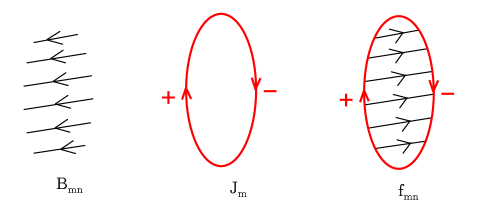
Figure 1: Backreaction of the open string field $f_{mn}$ to the presence of a current $J_{m}$ generated by a localized gauge trivial NSNS $B$–field.

Let us consider also the $S$–dual description of the above process. This involves looking at the RR shock wave

$$C^{\left(2\right)}=-\phi\left(x^{+}\right)dx^{2}\wedge dx^{3}\,.$$

In this case there is an induced current $J_{m}$, due to the Wess–Zumino coupling $-\int_{D3}C^{\left(2\right)}\wedge f$, which is non vanishing and is

$$J=\phi^{\prime}(x^{0})\,dx^{1}\,.$$

The Maxwell problem (1.1) is simply solved, again with retarded propagators, by

$$f=\phi(x^{0})\,dx^{0}\wedge dx^{1}\,,$$

so that one now sees that the noncommutativity in the future is due to the reaction of the open string $U(1)$ gauge potential to the current induced by the non vanishing RR field.

In these two examples, we have considered the process of turning on some closed string fields (always satisfying the equations of motion for the closed string) which are time dependent and which vanish in the far past. These fields induce a current $J$ which acts as a source for the open string fields, and we analyzed the unique reaction of the brane to this current by solving the corresponding Maxwell equation (1.1) using the physical requirement of causality, and therefore using retarded propagators. The example of the shock wave is particularly illuminating: one observes that, in order to obtain the standard noncommutative behavior to the future of the $S$–dual RR wave, which is expected by $S$–duality, we must incorporate the solution to equation (1.1) due to the current $J_{m}$. We should point out at this stage that the only principle we follow is a basic prescription on how to solve the open string equations uniquely, given a current $J$. We then notice that if we turn on two closed string field configurations, which are $S$–dual, then the final backgrounds including the backreaction of the brane will also be $S$–dual, as one expects.

The situation is not as straightforward when the closed string deformation does not vanish in the far past, and in particular is constant in spacetime. We shall thus mostly focus, from now on, on gauge trivial closed string deformations. We have seen with the first example that, for gauge trivial deformations which are localized in spacetime, nothing happens after one takes into account the open strings backreaction. On the other hand, as was just mentioned, we are interested in closed string deformations which are constant in spacetime. In the presence of a constant current, one does not have a simple physical principle (like retarded propagation of world–volume fields) to determine the backreaction of the open string, aside from the only requirement that:

(A) Whenever the induced current on the brane is the same, then the open string reaction should also be identical.

We have seen that, in the shock wave example, the final result compatible with (A) was also compatible with $S$–duality, in the sense that:

(B) Given two deformations of the closed string background which are $S$–dual then, after inserting a $D$–brane, the total backgrounds—i.e., the ones which include the backreaction of the open strings—are also $S$–dual.

On the other hand, just on the basis of Born–Infeld theory, it seems impossible to reconcile requirements (A) and (B) whenever the closed string perturbation is independent of time, as the following example shows. Consider a $D3$–brane in flat space stretched in the directions $0,1,2,3$, and let us turn on an NSNS field $B_{23}$. The current $J_{a}$ vanishes and we then use (A) to insist that the backreaction of the open strings should also vanish. The full system will then exhibit noncommutative behavior in the scattering processes of open string states, in the form of the well–known Moyal phase factors. The $S$–dual closed string background is, on the other hand, a constant RR $2$–form field $C_{01}$, which again induces no current. This time, however, the dynamics on the brane is completely unaltered since the background $U(1)$ field strength vanishes and since the Wess–Zumino action is a total derivative for gauge trivial RR fields, and therefore does not contribute to perturbative scattering amplitudes, unlike the previous situation.

In this paper we shall show that, if we consider the full string fields (open and closed) as opposed to only the low energy fields (meaning the massless fields in the low energy effective action with massive modes integrated out), then the situation is quite different and is in fact compatible with $S$–duality, in the sense of (B). In particular we shall show, both in the RNS and in the pure spinor covariant formulation of Berkovits, that constant NSNS and RR fields do induce a non vanishing current, which is the same for both the $B$ and the $C$ field backgrounds. Following (A) we must then only consider a single reaction from the open strings. We will then show, quite non–trivially, that the resulting total deformation of the background will be compatible with $S$–duality independently of the initial configurations of closed and open strings. More precisely, we will consider a $Dp$–brane stretched in directions $x^{0},\cdots,x^{p}$ with an initial background $U\left(1\right)$ flux $F_{ab}$, and we will consider turning on constant NSNS and RR fields $B$ and $C^{\left(q\right)}$. After computing the backreaction of the open strings following (A), we consider the final configuration which, quite naturally, corresponds to the original brane with a new gauge field

$$F_{ab}+\delta F_{ab}\left(F,B,C^{\left(q\right)}\right),$$

and possibly also with a rotated world–volume. We will then show that, in the case of a $D3$–brane, the result $\delta F_{ab}$ is compatible with $S$–duality, independently of $F$. To leading order, for fields $B$ and $C^{\left(2\right)}$ parallel to the brane, one has ($\star$ in here is Hodge duality on the brane)

$$\delta F=\frac{1}{2}\left(B-\star C^{\left(2\right)}\right)+\mathcal{O}\left(F\right),$$

which is compatible with $B\rightarrow C^{\left(2\right)},C^{\left(2\right)}\rightarrow-B$ and $\delta F\rightarrow\star\delta F$. The higher order terms in $\mathcal{O}\left(F\right)$ are computed explicitly and provide a strong check on the full construction.

This expression corresponds to the linear terms in an NSNS and RR noncommutative parameter $\Theta$. In order to compute the full nonlinear result one has to solve a complicated differential equation. Let us also comment on the factor of $\frac{1}{2}$ (which makes our result differ from the lore that one should have $F=B$). This factor arises due the fact that the world–sheet theory for the superstring (be it RNS or pure spinor) is quite different from the world–sheet theory for the bosonic string where there is no RR sector, the current $J$ vanishes, and one has $F=B$. Moreover, we should point out that the canonically normalized $F+B$ combination is still the $\sigma$–model gauge invariant expression to consider, as we show later in the paper.

This paper is organized as follows. We begin in section 2 with a brief summary of our results, for the reader who wishes to skip the technical details at first reading. In section 3 we describe the string field theoretic setting which allows us to describe open string physics in gauge trivial closed string backgrounds. This setting will be the basis for the calculations we shall perform in the following sections. We begin the calculations within the familiar RNS language [1, 2, 3, 4, 5, 6, 7, 8, 9, 10, 11, 12], in section 4. We shall focus our study on the case of a $D9$–brane in a constant RR $C$–field and observe that the boundary deformation, arising from the closed string background in the open string disk diagrams, precisely corresponds to that of an effective $\delta F$, as previously described. In order to analyze the most general picture, we switch to the pure spinor covariant formalism [13, 14, 15, 16, 17, 18, 19, 20, 21, 22, 23, 24, 25, 26, 27, 28, 29] in section 5. The power of this formalism allows us to fully describe $D$–brane physics in constant NSNS and RR potentials. The analysis of both sections 4 and 5 is done for background field strength $F_{ab}=0$ on the brane. In section 6 we consider the general case of finite $F_{ab}$, and set up the differential equation $\delta F_{ab}\,$ to determine the full nonlinear corrections to the background $F_{ab}$ and therefore to the open string parameters $G$ and $\Theta$ [30, 31, 32, 33, 34, 35, 36, 37, 38]. This last result then gives us the tools to perform the non–trivial check of $S$–duality in the $D3$–brane case, which we have discussed at length . We end in section 7 with some conclusions and open problems for future research. In appendix B it is shown how to solve a source equation describing the motion of an open superstring in a generic NSNS and RR closed string background.

2 Summary of Results

Let us summarize the main results we obtain in this paper. All formulae apply to type IIB theory, for infinitesimal $B$ and $C$–fields. The extension to type IIA is trivial.

We first consider a $Dp$–brane with no background $U\left(1\right)$ field strength $F=0$, immersed in a parallel $B$ field and in a general but constant RR potential

$$C=C_{\parallel}^{(q)}\wedge C_{\perp}^{(k)}\ ,$$

where $C_{\parallel}^{(q)}$ and $C_{\perp}^{(k)}$ are, respectively, a $q$ and a $k$–form parallel and transverse to the brane. Let also $\star$ be Hodge duality on the brane world–volume. The only non–trivial open string physics coming from the RR sector arises for the cases $(q,k)=(p-1,0)$ and $(q,k)=(p,1)$. In the first case, the two–form $\star C_{\parallel}^{(p-1)}$ is parallel to the brane and can be gauged away, together with the $B$–field, to a constant field strength

$$\delta F=\frac{1}{2}\left(B-\star C^{\left(p-1\right)}\right)\ ,$$

on the brane world–volume. Note that the normalization of the above fields is canonical, and that the non–standard factor of $1/2$ differs from the usually assumed result $\delta F=B$. This leads to the usual Moyal deformation also for RR fields and is compatible with $S$–duality, as discussed in the previous section. The other non–trivial case $(q,k)=(p,1)$ corresponds to a rotation of the brane world–volume. More precisely, if we define the two–form

$$\Omega=\star C_{\parallel}^{(p)}\wedge C_{\perp}^{(1)}\ ,$$

and if $x^{a}$ are the world–volume coordinates and $z_{i}$ the transverse scalars, then the displacement is

$$z_{i}=\frac{1}{2}\,x^{a}\,\Omega_{ai}\,.$$

We also consider $Dp$–branes in the presence of a finite background $U\left(1\right)$ field strength $F$. In the bulk of the paper we describe the general result, but here let us discuss the most relevant case, for $p=3$ with parallel background fields $B$ and $C^{\left(0\right)}$, $C^{\left(2\right)}$ and $C^{\left(4\right)}$. We discovered that the total induced variation $\delta F$ of the field strength $F$ is given by

$$\delta F\left(F,B,C^{\left(0\right)},C^{\left(2\right)},C^{\left(4\right)}\right)=\frac{1}{2}\left(B-\star C^{(2)}\right)-\frac{1}{2}F\wedge\star C^{\left(4\right)}+\frac{1}{2}\star F\wedge C^{\left(0\right)}+\cdots\ ,$$

where the dots represent terms of higher order in $F$ which can be computed explicitly. The most remarkable feature of the above result is its compatibility with $S$–duality, in the sense described qualitatively in the Introduction and to be made precise in section $6.2$. In fact, using the explicit formulae in this paper, we have checked $S$–duality to all orders in $F$! This leads to an $S$–dual invariant prescription for a Moyal noncommutative deformation.

3 Basic String Field Theory Setting

In order to understand the issue more clearly, we first need to discuss, from a general and qualitative point of view, what we mean by the motion of an open string in a closed string background, and in particular in a gauge trivial closed string background.

In general, strings at weak coupling are described by an open–closed string field theory action [42, 43, 44, 45] which is written in terms of a closed and an open string field, $\Psi$ and $\Phi$ (in bosonic string theory, respectively of ghost number $2$ and $1$), and which is of the general form

$$\frac{1}{g^{2}}S_{c}+\frac{1}{g}S_{o}+\frac{1}{g}S_{oc}\ ,$$

where $S_{c}$ represents the closed string field theory action, coming from interactions with sphere diagrams, and where $S_{o}$ and $S_{oc}$ correspond to the open string field action and to the interaction terms between open and closed strings, and are related to disk diagrams. This explains the different powers of the string coupling in front of the various terms. Focusing on the linearized classical equations of motion in the free $g\rightarrow 0$ limit, we have in general the equations

$$Q\Psi = 0\ ,$$ (3.2)

$$Q\Phi = -J\ ,$$ (3.3)

where $Q$ is the (either open or closed) BRST operator, and where we have defined

$$J\equiv\pi\left(\Psi\right).$$

The map $\pi$ relates closed to open string states. One can think of this map as a projection map, projecting the closed string vertex operators in the world–sheet bulk to the world–sheet boundary (implementing appropriate boundary conditions between left and right movers). Its detailed properties depend on the specific string field theory in question, but $\pi$ generically will preserve ghost number and will have the property that

$$Q\pi\left(\Xi\right)=\pi\left(Q\Xi\right).$$

It is clear that equations (3.2) and (3.3) are asymmetric and one can, in particular, choose $\Psi$ to satisfy the closed string equations of motion completely forgetting about the open string sector (this is true also in the interacting theory). This asymmetry is directly related to the different powers of $g$ corresponding to closed and open string interactions, and it is the very reason why one can talk about open strings in a closed string background but not vice–versa. Given a solution, $\Psi$, in order to find a consistent vacuum one must solve equation (3.3) for $\Phi$. We now recall that, for the massless bosonic sector, the on–shell equation $Q\Phi=0$ corresponds to the free Maxwell equations of motion. This implies that we should consider $J$ as a source term for the Maxwell equations, or as a current. Then, current conservation is nothing but the statement that $QJ=\pi\left(Q\Psi\right)=0$. These facts are the generalization, using the full string field, of the setup described in the introduction, and we shall see, in the following sections, concrete examples both in the RNS and in the pure spinor formalism.

Let us now consider the gauge invariance of the string field theory equations of motion, focusing on the linear part of the gauge transformations (since we are looking only at the linear equations of motion in this discussion). We clearly have the usual open string gauge transformations $\Phi\rightarrow\Phi+Q\kappa$. We will be, on the other hand, more interested in the closed string gauge transformations which read, in the presence of the open string sector,

$$\Psi\rightarrow\Psi-Q\eta\ ,\ \ \ \ \ \ \ \ \ \ \ \ \ \ \ \ \ \ \ \ \ \ \ \ \ \ \ \ \ \Phi\rightarrow\Phi+\pi\left(\eta\right)\ .$$ (3.4)

Clearly any two vacua related by the above gauge transformations will be completely equivalent and will yield the same physical results.

We may now discuss more clearly what we mean by open strings propagating in a gauge trivial closed background. Consider a closed string background given by

$$\Psi=Q\eta\ .$$

As we pointed out, one can choose this background before talking about open strings. As a second step we need to solve equation (3.3) for the open string field. Denoting the solution with $\Phi_{r}$, we need to solve

$$Q\Phi_{r}=-J=-Q\Phi_{c}\ ,$$ (3.5)

where we have defined the open string state

$$\Phi_{c}\equiv\pi\left(\eta\right).$$ (3.6)

Clearly one solution of (3.5) is given by $\Phi=-\Phi_{c}$. Recalling the first example in the introduction, this solution will be the natural one whenever $\Psi$ is localized in spacetime. This case is, on the other hand, quite uninteresting since the vacuum $\Psi=Q\eta$, $\Phi=-\pi\left(\eta\right)$ is a gauge transform of the $\Psi=\Phi=0$ vacuum. For more general configurations, as we have already discussed at length in the introduction, we must have a general principle on how to solve (3.5), which must be compatible at least with requirement (A) in the introduction. At any rate, we will later discuss more generally how to solve equation (3.5), but for now we just denote with $\Phi_{r}$ the solution, which we assume unique given $J$. We have the new, in general physically different vacuum $\Psi=Q\eta$, $\Phi=\Phi_{r}$. We can then apply the gauge transformation (3.4) to bring the solution to the form

$$\Psi = 0\,,$$

$$\Phi = \Phi_{c}+\Phi_{r}\,.$$

In this way, we can associate to any gauge trivial closed string state $\Psi=Q\eta$ a corresponding on–shell deformation of the open string $\Phi_{c}+\Phi_{r}$ by using equations (3.6) and (3.5). We therefore have a map which sends gauge trivial closed string deformations into on–shell physical open string deformations. We want to show that, whenever $\Psi$ and $\widetilde{\Psi}$ are $S$–dual closed gauge–trivial deformations, then our procedure will yield $S$–dual open string deformations $\Phi_{c}+\Phi_{r}$ and $\widetilde{\Phi}_{c}+\widetilde{\Phi}_{r}$, under the requirement (A) that equal currents $J$ go into equal solutions $\Phi_{r}$ of (3.5). We will show that this is possible for the case of constant NSNS and RR gauge field backgrounds. A word on the notation. We have divided the open string field $\Phi$ in a part coming from the closed string and a part coming from the reaction of the open string. This explains the choice of subscripts $\Phi_{c}$ and $\Phi_{r}$.

To illustrate this procedure in a familiar setting, let us consider the bosonic string and show how to obtain the well–known (infinitesimal) deformation of $F=B$. This will make clear, in a simplified case, how the above reasoning works. Given the constant $B$–field bosonic closed string background, described at zero momentum by

$$\Psi=\frac{1}{2}\,c\overline{c}\left[B_{mn}\partial X^{m}\overline{\partial}X^{n}\right],$$

it is simple to compute that the corresponding current will vanish, $J=\pi(\Psi)=0$. Indeed, the $\pi$ map brings the closed string vertex operator to the boundary of the world–sheet, where $c=\overline{c}$. Following the procedure outlined above one now computes, in a unique way, the open string reaction via $Q\Phi_{r}=-J=0$, which yields $\Phi_{r}=0$. The open string deformation will thus be given by $\Phi=\Phi_{c}+\Phi_{r}=\Phi_{c}$, where one still needs to find $\Phi_{c}=\pi(\eta)$. First observe that with

$$\eta=\frac{1}{4}\,B_{mn}\left[X^{m}\,\overline{c}\overline{\partial}X^{n}-c\partial X^{m}\,X^{n}\right]$$

it follows that $\Psi=Q\eta$. Then, it is simple to compute the open string deformation as

$$\Phi=\pi(\eta)=\frac{1}{2}\,B_{mn}\,X^{m}\partial X^{n}.$$

This is the expected final result of $F=B$ open string deformation, for the bosonic string. In the superstring case one will find that the current $J$ is actually non–vanishing (though equal in the two cases of NSNS and RR deformations), and the whole story will be very different from this simple bosonic case. In fact, $\Phi_{c}$ alone will no longer be a solution of the open string equations of motion, and one will have to endure a much harder analysis in order to add the $\Phi_{r}$ contribution.

We now have the general framework to address our main problem at hand. We need to understand better, in specific cases, the map $\pi$ and, more importantly, how to solve equation (3.5) or, more generally, equation (3.3). We shall first start by performing such an analysis in the familiar setting of the RNS formalism, and will only later proceed to use the more powerful pure spinor covariant formalism, where the whole picture will become much clearer.

4 Analysis in the RNS Formalism

In the RNS formulation of the superstring [1, 2, 3, 4] the matter fields organize into the action

$$\frac{1}{2\pi}\int d^{2}z\ \left(\frac{2}{\alpha^{\prime}}\partial X^{\mu}\bar{\partial}X_{\mu}+\psi^{\mu}\bar{\partial}\psi_{\mu}+\overline{\psi}^{\mu}\partial\overline{\psi}_{\mu}\right),$$

whereas the ghost fields are the usual $bc$ and $\beta\gamma$ systems. It is standard to fermionize the $\beta\gamma$ superconformal ghosts as $\beta=\partial\xi e^{-\phi}$ and $\gamma=\eta e^{\phi}$. Also, we shall work in $\alpha^{\prime}=2$ units. The BRST operator $Q=Q_{L}+Q_{R}$ naturally decomposes into three pieces [1],

$$Q_{L}=Q_{0}+Q_{1}+Q_{2}\ ,$$ (4.7)

labeled by their spinor ghost charges

$$Q_{0} = \oint\frac{dz}{2\pi i}\ \left[c\left(T_{X}+T_{\psi}+T_{\eta\xi}+T_{\phi}\right)+c\partial cb\right]\ ,$$

$$Q_{1} = \frac{1}{2}\oint\frac{dz}{2\pi i}\ e^{\phi}\eta\psi^{\mu}\partial X_{\mu}\ ,$$

$$Q_{2} = \frac{1}{4}\oint\frac{dz}{2\pi i}\ b\eta\partial\eta e^{2\phi}\ .$$

The BRST operator has total ghost number $1$ and total picture number $0$.

4.1 Vertex Operator $\Psi$ for the $B$ and $C$–Fields in Superstring Theory

In this section we analyze the vertex operators $\Psi_{B}$ and $\Psi_{C}$ for a constant $B$–field and a constant $C$–field.

We recall first that scattering amplitudes on the disk are saturated with the insertion of three ghost fields $c,\overline{c}$ and with a total picture number of $(-2)$ [4]. In particular, for closed string vertex operators, picture number is counted by summing the left and right sector picture numbers $p$, ${\overline{p}}$. We shall subsequently be interested in world–sheet bulk vertex operators $\Psi$ such that $p+\overline{p}=-2$. Therefore, if one considers the disk interaction of $n$ gluons and $2m$ gluinos, in the presence of the closed vertex $\Psi$, the total picture number for the gluons and the gluinos must vanish and the correlator will look schematically like

$$\langle\;\underbrace{{\mathcal{V}}_{(0)}\;\cdots\;{\mathcal{V}}_{(0)}}_{n}\;\underbrace{{\mathcal{V}}_{(+\frac{1}{2})}\;{\mathcal{V}}_{(-\frac{1}{2})}\;\cdots\;{\mathcal{V}}_{(+\frac{1}{2})}\;{\mathcal{V}}_{(-\frac{1}{2})}}_{2m}\;\Psi\;\rangle\ .$$

The $B$–field vertex operator in the $(-1,-1)$ picture is standard and is given, at zero momentum, by the expression

$$\Psi^{B}=-c\overline{c}\left[B_{mn}\psi^{m}\overline{\psi}^{n}e^{-\phi}e^{-\overline{\phi}}\right].$$ (4.8)

Consider now the $C$–field bulk vertex operator. In the standard $(-\frac{1}{2},-\frac{1}{2})$ symmetric picture this vertex operator will contain the RR field strength $F_{q+1}=dC_{q}$, and not the RR gauge potential $C_{q}$, as is well known, for example, from many $D$–brane scattering calculations [5, 6, 7, 8]. In order to obtain a vertex operator which depends on the RR gauge potential one needs to change to an asymmetric picture [9, 10, 11]. Due to the nature of our calculations, this asymmetric picture vertex operator is precisely the one we are interested in. It has, as we shall see, total picture number $(-2)$ and it is therefore the natural companion of the operator $\Psi^{B}$ for constant $B$–field. We will present explicit formulae for type IIB, the extension to IIA being trivial.

Let us first introduce some notation for the RR potentials. For spinor conventions, please refer to appendix A. We let $C_{m_{1}\cdots m_{q}}$, with $q$ even, be the RR $q$–form potential, and we define as usual the bi–spinor

$$C_{\alpha}{}^{\beta}=\sum_{q\mathrm{\ even}}\frac{1}{q!}C_{m_{1}\cdots m_{q}}\left(\gamma^{m_{1}\cdots m_{q}}\right)_{\alpha}{}^{\beta}\ ,$$

and similarly for the dual version $C^{\alpha}{}_{\beta}$. Also, we will find convenient to use, together with $C^{\alpha}{}_{\beta}$, its transpose ${\overline{C}}_{\alpha}{}^{\beta}=C^{\beta}{}_{\alpha}$ given by

$${\overline{C}}_{\alpha}{}^{\beta}=\sum_{q\mathrm{\ even}}\frac{(-)^{\frac{q}{2}}}{q!}C_{m_{1}\cdots m_{q}}\left(\gamma^{m_{1}\cdots m_{q}}\right)_{\alpha}{}^{\beta}\ .$$

The $C$–field vertex operator $\Psi^{C}$, at zero momentum, is a sum of two pieces at picture number $(-\frac{3}{2},-\frac{1}{2})$ and $(-\frac{1}{2},-\frac{3}{2})$ [9, 10, 11]

$$\Psi^{C}=\frac{1}{16}c\overline{c}\left[S^{\alpha}\ {{C}_{\alpha}}^{\beta}\overline{S}_{\beta}e^{-\frac{3}{2}\phi}e^{-\frac{1}{2}\overline{\phi}}-S_{\alpha}\ {{C}^{\alpha}}_{\beta}\overline{S}^{\beta}e^{-\frac{1}{2}\phi}e^{-\frac{3}{2}\overline{\phi}}\right]\,,$$ (4.9)

where $S$ are the spin fields.

In the language of section 3, we now have the closed string field $\Psi$. It is pure gauge, so we proceed to compute the corresponding open string current $J=\pi(\Psi)$ (section 4.2) and the BRST potential $\eta$ and $\Phi_{c}=\pi(\eta)$ (section 4.3).

4.2 Boundary OPE’s for $\Psi^{B}$ and $\Psi^{C}$: Computation of the Current $J$

In this section we wish to compute the open string current $J=\pi(\Psi)$ generated by the closed string field $\Psi$. Therefore we must introduce open strings by restricting the CFT to the upper half complex plane ${\mathbb{H}}$ and by imposing boundary conditions on $\partial{\mathbb{H}}$. We will then define the closed–open projection $\pi(\Psi)$ to be simply the boundary OPE of the operator $\Psi$ as it approaches $\partial{\mathbb{H}}$. This definition is clearly valid only if the OPE is non–singular, which will be true for the applications which follow.

We will discuss in this section the specific case of the $D9$–brane in type IIB. The more general cases are discussed in section 5 using the covariant formalism. The $D9$–brane boundary conditions on $\partial{\mathbb{H}}$ are

$$\overline{\partial}X^{m} = \partial X^{m}\,,\ \ \ \ \ \ \ \ \ \ \ \ \overline{\psi}^{m}=\psi^{m}\,,$$

$$\overline{S}^{\alpha} = S^{\alpha}\,,\ \ \ \ \ \ \ \ \ \ \ \ \ \ \ \overline{S}_{\alpha}=S_{\alpha}\,,$$

together with the boundary conditions for the ghost fields,

$$\overline{{\mathrm{Ghost}}}={\mathrm{Ghost}}\,.$$

Let us start by computing the current $J^{B}=\pi(\Psi^{B})$ related to a constant $B$–field background. As we discussed above the definition of $\pi$ implies that we must compute the following OPE

$$J^{B}=\lim_{z\to\bar{z}}\Psi^{B}(z,\bar{z})\ .$$

Using the boundary conditions we get that

$$\lim_{z\to\bar{z}}\Psi^{B}(z,\bar{z}) = B_{mn}\ \lim_{z\to\bar{z}}\ \left(c\partial c(\bar{z})+\frac{1}{2}\left(z-\bar{z}\right)c\partial^{2}c(\bar{z})+{\mathcal{O}}(z-\bar{z})^{2}\right)\cdot$$

$$\cdot\left(\frac{g^{mn}}{z-\bar{z}}-g^{mn}{\partial}\phi(\bar{z})+\psi^{m}\psi^{n}(\bar{z})+{\mathcal{O}}(z-\bar{z})\ \right)e^{-2\phi(\bar{z})}\ .$$

Besides the standard OPE’s [1], we have used the relation

$$\psi^{m}(z)\psi^{n}(w)=\frac{g^{mn}}{z-w}+:\psi^{m}\psi^{n}:(w)+\cdots\ .$$

The final result for the current $J^{B}$ reads

$$J^{B}=B_{mn}\ c\partial c\ \psi^{m}\psi^{n}\ e^{-2\phi}\ .$$ (4.10)

Note that $J^{B}$ is an open string operator at picture number $(-2)$ and ghost number $(+2)$ as expected.

We now turn to the $C$–field case. The treatment is identical to the previous situation, with the exception that the analysis involves the OPE’s of the spin fields

$$S^{\alpha}(z)S_{\beta}(w)\sim(z-w)^{-\frac{5}{4}}\ \delta^{\alpha}{}_{\beta}+(z-w)^{-\frac{1}{4}}\ \frac{1}{2}{\left[\gamma_{mn}\right]^{\alpha}}_{\beta}\ \psi^{m}\psi^{n}(w)+\cdots\ .$$

We may then compute the limit

$$\lim_{z\to\bar{z}}\Psi^{C}(z,\bar{z}) = -\frac{1}{16}{C}_{\alpha}{}^{\beta}\ \lim_{z\to\bar{z}}\ \left(c\partial c(\bar{z})+\frac{1}{2}\left(z-\bar{z}\right)c\partial^{2}c(\bar{z})+{\mathcal{O}}(z-\bar{z})^{2}\right)\cdot$$

$$\cdot\Big{(}\frac{\delta^{\alpha}{}_{\beta}}{z-\bar{z}}-\frac{3}{2}\delta^{\alpha}{}_{\beta}\ {\partial}\phi(\bar{z})+\frac{1}{2}{\left[\gamma_{mn}\right]^{\alpha}}_{\beta}\ \psi^{m}\psi^{n}(\bar{z})+{\mathcal{O}}(z-\bar{z})\Big{)}e^{-2\phi(\bar{z})}-\cdots\ ,$$

where the terms in $\cdots$ are similar and come from the picture number $(-\frac{1}{2},-\frac{3}{2})$ part of $\Psi^{C}$. To get a regular OPE we will assume that ${C}_{\alpha}{}^{\alpha}=0$. In this case we conclude that

$$J^{C} = -\frac{1}{32}\left({C}_{\alpha}{}^{\beta}\ {\left[\gamma_{mn}\right]^{\alpha}}_{\beta}\ -{C}^{\alpha}{}_{\beta}\ {\left[\gamma_{mn}\right]_{\alpha}}^{\beta}\ \right)\ c\partial c\ \psi^{m}\psi^{n}e^{-2\phi}$$ (4.11)

$$= \frac{1}{32}{\rm Tr}\left[(C+{\overline{C}})\gamma_{mn}\right]\ c\partial c\ \psi^{m}\psi^{n}e^{-2\phi}\ .$$ (4.12)

Clearly, the only RR–field that contributes to $J^{C}$ is the $8$–form potential (since the sum $C+{\overline{C}}$ does not include the $2$–form potential). Moreover it is easy to show that $J^{C}$ has the same form of $J^{B}$ with an effective $B$–field given by

$$B_{\rm eff}=-\frac{1}{64}{\rm Tr}\left[(C+{\overline{C}})\gamma_{mn}\right]dx^{m}\wedge dx^{n}=-\star C^{(8)}.$$

This is the first instance of the results we have discussed in section 1.

Two comments are now in order. Firstly, we are discussing only the $D9$–brane case, for clarity of exposition. We will discuss the general case in the (simpler) framework of the covariant formalism, which we shall describe in section 5. Secondly, we should note that these results are only valid to linear order in the background fields. In order to determine the full nonlinear RR noncommutativity extra work is required. In fact, using the general results in the covariant formalism one can write down a differential equation for the noncommutativity parameter, as the background fields $B$ and $C$ are turned on. When one has only $B$–field the full non–linear result is known. We shall discuss the non–linear result with both fields in section 6.

4.3 BRST Potentials for Vertex Operators: Computing $\eta$ and $\Phi_{c}$

In the last section we have studied the open string current $J$. Since we are dealing with constant $B$ and $C$–fields, we expect that the vertex operators (4.8) and (4.9) are BRST exact. In this section we address the question of finding the BRST potential, $\eta$, for these operators, satisfying $\Psi=Q\eta$, and then study their boundary OPE, $\Phi_{c}=\pi(\eta)$.

Let us begin with the vertex operator for the $B$–field, (4.8). Counting of conformal dimension, ghost and picture numbers, suggests that one should consider the operator of ghost number $(-1)$ (concentrating on the left–movers for the moment)

$$2c\partial\xi e^{-2\phi}f(X)\,.$$

The only non–trivial commutation is with the $Q_{1}$ component of the BRST operator, which will produce

$$\left[Q_{1},2c\partial\xi e^{-2\phi}f(X)\right]=c\psi^{m}e^{-\phi}\partial_{m}f(X)\,.$$

If we introduce an one–form $\Lambda$ such that $B=d\Lambda$ with $\partial\cdot\Lambda=\square\Lambda=0$ (for example $2\Lambda_{n}=x^{m}B_{mn}$) it is quite easy to show that

$$\Psi^{B}=\left[Q_{L}+Q_{R},\eta^{B}\right],$$

where

$$\eta^{B}=-2\Lambda_{m}(X)\ c{\overline{c}}\left[\partial\xi e^{-2\phi}\ \overline{\psi}^{m}e^{-\overline{\phi}}+\psi^{m}e^{-\phi}\ \bar{\partial}\overline{\xi}e^{-2\overline{\phi}}\right].$$

To compute $\Phi_{c}=\pi(\eta)$ we take the boundary OPE of the BRST potential and we get

$$\Phi^{B}_{c}=\lim_{z\to\bar{z}}\eta^{B}(z,\bar{z})=2\Lambda_{m}(X)\ c\partial c\ \psi^{m}\ \partial\phi\partial\xi\ e^{-3\phi}\ .$$ (4.13)

Next, we turn our attention to the $C$–field vertex operator (4.9). Conformal dimension, and ghost and picture number counting now tell us that the natural operator to consider is

$$2\ c\partial c\ \partial\xi\partial^{2}\xi\ S^{A}\ e^{-\frac{7}{2}\phi}\ f(X)\ .$$

This time the relevant non–trivial commutation relation is with the $Q_{2}$ component of the BRST operator (4.7), where one finds as expected

$$\left[Q_{2},2\ c\partial c\ \partial\xi\partial^{2}\xi\ S^{A}\ e^{-\frac{7}{2}\phi}\ f(X)\right]=c\ S^{A}\ e^{-\frac{3}{2}\phi}\ f(X)\ .$$

Thus, if one considers the operator

$$\eta^{C}=-\frac{1}{8}c\partial c\ \partial\xi\partial^{2}\xi\ e^{-\frac{7}{2}\phi}\ S^{\alpha}\ C_{\alpha}{}^{\beta}\ \overline{c}\ \overline{S}_{\beta}\ e^{-\frac{1}{2}\overline{\phi}}+\cdots\ ,$$

(the $\cdots$ are the symmetric term with left and right movers interchanged) commutation of $Q_{L}+Q_{R}$ with this operator then yields the $C$–field vertex operator

$$\Psi^{C}=\left[Q_{L}+Q_{R},\eta^{C}\right].$$

As we take the boundary OPE of this BRST potential one finds

$$\Phi^{C}_{c}=\lim_{z\to\bar{z}}\eta^{C}(z,\bar{z})=\frac{1}{32}{\rm Tr}\left[(C+{\overline{C}})\gamma_{mn}\right]\ c\partial c\partial^{2}c\ \partial\xi\partial^{2}\xi\ \psi^{m}\psi^{n}(z)\ e^{-4\phi}\,.$$ (4.14)

Observe that, as expected, both (4.13) and (4.14) live at picture $(-2)$.

To conclude the general procedure discussed in section 3, we must now understand the reaction term $\Phi_{r}$ of the open strings, and the total deformation $\Phi_{c}+\Phi_{r}$. In order to do so, we analyze in the next section the gluon vertex operator at picture number $(-2)$.

4.4 The Gluon Vertex Operator at Picture Number $(-2)$

The boundary operators we have obtained in the previous section are

$$a_{m}(X)\ c\partial c\ \psi^{m}\ \partial\phi\partial\xi\ e^{-3\phi}\ ,$$

and

$$f_{mn}(X)\ c\partial c\partial^{2}c\ \partial\xi\partial^{2}\xi\ \psi^{m}\psi^{n}\ e^{-4\phi}\ .$$

Recall that the ghost number assignment of $e^{q\phi}$ is $q$ [1], so that both these operators are at ghost number $(-1)$ and picture number $(-2)$. The question we face is whether picture raising will bring a linear combination of these operators to the canonical gluon vertex operator at picture number $(-1)$

$$\Phi_{(-1)}=2a_{m}(X)\ c\psi^{m}\ e^{-\phi}\ .$$ (4.15)

Let us consider the following ansätz for the gluon vertex operator at picture number $(-2)$,

$$\Phi_{(-2)} = k_{1}\ a_{m}(X)\ c\partial c\ \psi^{m}\ \partial\phi\partial\xi\ e^{-3\phi}$$

$$+k_{2}\ f_{mn}(X)\ c\partial c\partial^{2}c\ \partial\xi\partial^{2}\xi\ \psi^{m}\psi^{n}\ e^{-4\phi}\ ,$$

where $k_{1}$ and $k_{2}$ are two constants to be determined and, at the moment, we are assuming no relation between $a_{m}$ and $f_{mn}$. We need to show that the picture raising operation will take $\Phi_{(-2)}$ to $\Phi_{(-1)}$ or, more specifically, that

$$\Phi_{(-1)}=\left[Q,2\xi\Phi_{(-2)}\right].$$

As expected, we will have to impose that $f=da$ as well as the on–shell relations $\partial\cdot a=0=\square a$ for the gluon field.

We shall begin with the piece proportional to $a_{m}$. Assuming $\square a=0$, it is simple to realize that the commutation with the $Q_{0}$ component of (4.7), in the formula above, will vanish. To analyze the commutation with $Q_{1}$, one has to use the fermion OPE,

$$\psi^{m}(z)\psi^{n}(w)=\frac{g^{mn}}{z-w}+:\psi^{m}\psi^{n}:(w)+\cdots\,.$$

The term which arises from the singular part above will be proportional to $\partial\cdot a$, which we take to be zero in the Lorentz gauge. The term that arises from the normal ordered piece is non–vanishing and reads

$$\left[Q_{1},2\xi\ a_{m}\ c\partial c\ \psi^{m}\ \partial\phi\partial\xi\ e^{-3\phi}\right]=-\Big{(}\partial_{m}a_{n}-\partial_{n}a_{m}\Big{)}\ \xi c\partial c\psi^{m}\psi^{n}e^{-2\phi}\ .$$

At first sight the above result seems strange, as the right hand side is a vertex operator off the small Hilbert space. As we shall see in a moment, this term will cancel out in the final expression exactly when $\Phi_{(-2)}$ is BRST closed. This is simple to understand since the terms proportional to $\xi$ arise, schematically, from $[Q,2\xi\Phi_{(-2)}]\simeq 2\xi[Q,\Phi_{(-2)}]+\cdots$ and vanish when $[Q,\Phi_{(-2)}]=0$. As to the commutation with the last component of (4.7), $Q_{2}$, it yields the expected expression for the gluon vertex operator at the canonical $(-1)$ picture,

$$\left[Q_{2},2\xi\ a_{m}\ c\partial c\ \psi^{m}\ \partial\phi\partial\xi\ e^{-3\phi}\right]=\ a_{m}\ c\psi^{m}e^{-\phi}\ .$$

Let us now turn to the term proportional to $f_{mn}$ in $\Phi_{(-2)}$. Again, with $\square f=0$, one quickly shows that the commutation with the $Q_{0}$ component of the BRST operator vanishes. Commutation with the $Q_{1}$ component, on the other hand, yields a term proportional to the Yang–Mills equation of motion $\partial^{m}f_{mn}$, which vanishes for $f=da$ with an on–shell gluon. The final commutation with the $Q_{2}$ component of the BRST operator results in an operator that is again off the small Hilbert space, namely

$$\left[Q_{2},2\xi(z)\ f_{mn}\ c\partial c\partial^{2}c\ \partial\xi\partial^{2}\xi\ \psi^{m}\psi^{n}\ e^{-4\phi}\right]=-2\ f_{mn}\ \xi c\partial c\psi^{m}\psi^{n}e^{-2\phi}\ .$$

Because we are looking for the physical gluon vertex operator, at picture $(-1)$, we cannot allow for terms which are outside the small Hilbert space, so we require that the two terms proportional to $\xi(z)$ cancel with each other. This requirement is fulfilled when

$$k_{1}+2k_{2}=0$$

and $f=da$. Moreover, under this condition, as we discussed above, the state $\Phi_{(-2)}$ is BRST closed. In conclusion, fixing the overall normalization, the gluon vertex operator at picture $(-2)$ is simply

$$\Phi_{(-2)} = \ 2\,a_{m}(X)\ c\partial c\ \psi^{m}\ \partial\phi\partial\xi\ e^{-3\phi}$$

$$-\,f_{mn}(X)\ c\partial c\partial^{2}c\ \partial\xi\partial^{2}\xi\ \psi^{m}\psi^{n}\ e^{-4\phi}\ .$$

We shall, moreover, denote with $\Phi_{(-2)}(F)$ the gluon vertex operator corresponding to a constant field strength $f_{mn}(X)=F_{mn}$, $2a_{m}(X)=-F_{mn}X^{n}$.

To conclude the argument and to prove that, in the presence of a $C$–field (in particular in the example we are discussing, of a $8$–form RR potential), the open strings react and behave as in the presence of an effective $B$–field $B_{\rm eff}=-\star C^{(8)}$, we must solve the source equation $Q\Phi_{r}=-J$. We shall later develop a general strategy to solve this equation in the covariant formalism, so for the moment we are forced to borrow one result from section 5, which is based both on this general formalism as well as on arguments of $S$–duality. More precisely, we will show in section 5.5 that, in the presence of a $B$–field, the total boundary deformation will be

$$\Phi_{c}^{B}+\Phi_{r}^{B}=\frac{1}{2}\Phi_{(-2)}(B)\ .$$

We remark that in this superstring case there is an extra factor of $1/2$, which differs from the usual result given in [30, 31, 32, 33, 34, 35, 36, 37, 38], but is unequivocally determined within the pure spinor formalism. Given the above equation, the reaction term $\Phi^{B}_{r}$ to the current $J^{B}$ must be given by

$$\Phi_{r}^{B} = -\frac{1}{2}B_{mn}X^{m}\ c\partial c\ \psi^{n}\ \partial\phi\partial\xi\ e^{-3\phi}$$

$$-\frac{1}{2}\ B_{mn}\ c\partial c\partial^{2}c\ \partial\xi\partial^{2}\xi\ \psi^{m}\psi^{n}\ e^{-4\phi}\ .$$

Note that the relative sign between the two terms is different from the one in $\Phi_{(-2)}$. This must be so since $\Phi_{(-2)}$ is BRST closed, whereas $Q\Phi_{r}=-J$. In the $C$–field case one has an identical current $J$ (up to an overall sign and the replacement $B\to B_{\rm eff}$), and therefore the reaction must be identical. Thus, we conclude that

$$\Phi_{c}^{C}+\Phi_{r}^{C}=\frac{1}{2}\Phi_{(-2)}(B_{\rm eff})\ ,$$

as we wanted to show.

One would like to develop better these arguments, in a context where RR fields appear naturally, in order to fully understand the most general cases. This shall be studied next, in the context of the pure spinor formalism, which allows for a manifest super Poincaré covariant quantization of the superstring and where RR fields can be studied most simply.

5 Analysis in the Covariant Formalism

Let us start by reviewing the basics of the pure spinor covariant formalism, as developed by Berkovits in an extensive list of papers [13, 14, 15, 16, 17, 18, 19, 20, 21, 22, 23, 24, 25]. We shall write all the formulae for type IIB string theory, but the generalization to type IIA is straightforward.

5.1 The Underlying Conformal Field Theory

In this section we recall the conformal field theory underlying the covariant formalism in flat space. We shall again use units such that $\alpha^{\prime}=2$. First of all, we have the usual matter part

$$\frac{1}{2\pi}\int d^{2}z\,\partial x^{m}{\overline{\partial}}x^{n}\,g_{mn}\ ,$$

of central charge $+10$. The spacetime coordinates $x^{m}$ are completed, to form the IIB ten dimensional superspace, with the addition of the fermionic chiral spinor coordinates $\theta^{\alpha}$, $\overline{\theta}^{\alpha}$ (see appendix A for spinor conventions). These fermionic coordinates are promoted to conformal fields of the underlying CFT, together with their respective conjugate momenta $p_{\alpha}$, $\overline{p}_{\alpha}$, with the action

$$\frac{1}{\pi}\int d^{2}z\,\left(p_{\alpha}\overline{\partial}\theta^{\alpha}+\overline{p}_{\alpha}\partial\overline{\theta}^{\alpha}\right)\,.$$

The fields $\theta^{\alpha}$ and $p_{\alpha}$ form $16$ fermionic holomorphic $bc$ systems of conformal dimension $0$ and $1$ respectively, which contribute $-32$ to the central charge ($-2$ for each of the $16$ pairs). The same holds for the pairs $\overline{\theta}^{\alpha}$, $\overline{p}_{\alpha}$ on the anti–holomorphic side. Finally we have the bosonic pure spinors $\lambda^{\alpha}$, $\overline{\lambda}^{\alpha}$ together with their conjugate pairs $w_{\alpha}$, $\overline{w}_{\alpha}$ and with an action of the sort

$$``\;\frac{1}{\pi}\int d^{2}z\,\left(w_{\alpha}\overline{\partial}\lambda^{\alpha}+\overline{w}_{\alpha}\partial\overline{\lambda}^{\alpha}\right)\;"\ .$$ (5.16)

We should think of the pairs $\lambda^{\alpha}$ and $w_{\alpha}$ as bosonic $\beta\gamma$ systems of conformal dimension $0$ and $1$. The reason for the quotation marks around the above action is that the fields $\lambda$ and $\overline{\lambda}$ are not free, but constrained to be pure spinors satisfying the equation

$$\lambda\gamma^{m}\lambda=0=\overline{\lambda}\gamma^{m}\overline{\lambda}\ .$$ (5.17)

Without this constraint, the action (5.16) would contribute $+32$ to the central charge. However, given the above constraints, the number of degrees of freedom is reduced and the contribution to the central charge is $+22$, as expected for a critical string theory. One of the useful results of the covariant formalism is that one can actually solve the constraint (5.17) using only free fields, in which case $\lambda$ and $\overline{\lambda}$ become composite fields and the action (5.16) is replaced by a honest action of the underlying free fields. We shall not need the details of this construction, which can be found in [14]. For future reference, and to fix normalizations, let us record some of the basic OPE’s of the CFT

$$\partial x^{m}\left(z\right)\partial x^{n}\left(w\right) \sim -\frac{g^{mn}}{\left(z-w\right)^{2}}\ ,$$

$$p_{\alpha}\left(z\right)\,\theta^{\beta}\left(w\right) \sim \frac{\delta_{\alpha}{}^{\beta}}{z-w}\ .$$

5.2 BRST Operator and Closed String Spectrum

Central to the construction of any string theory is the description of physical states in terms of BRST cohomology, and the same holds true for the covariant formulation [14, 16, 20]. More precisely, the conserved BRST current on the world–sheet is given, in terms of the basic fields given above, by

$$J_{BRST}=\left(\lambda d\right)dz-\left(\overline{\lambda}\overline{d}\right)d\overline{z}\ ,$$

where the spinor current $d_{\alpha}$ is defined by

$$\lambda d=\lambda p-\left(\lambda\gamma^{m}\theta\right)\partial x_{m}-\left(\lambda\gamma^{m}\theta\right)\left(\theta\gamma_{m}\partial\theta\right)$$

and a similar equation holds for $\overline{d}_{\alpha}$. The BRST operator is then given by

$$Q=Q_{L}+Q_{R}=\frac{1}{2\pi i}\oint J_{BRST}\ .$$

The second ingredient in the construction of the physical spectrum is the grading of the states by ghost number $g=g_{L}+g_{R}$. This is defined by declaring $g_{L}(\lambda)=g_{R}({\overline{\lambda}})=1$ and $g_{L}(w)=g_{R}({\overline{w}})=-1$, with the conformal vacuum of ghost number zero as usual. With this definition, $g_{L}(Q_{L})=g_{R}(Q_{R})=1$ as expected. Then, the closed string states are identified with the BRST cohomology at total ghost number $g=2$.

The massless spectrum, in the covariant formulation, is particularly simple as states are constructed uniquely from the zero modes of the fields and therefore are represented by functions in type II superspace $(x^{m},\theta,{\overline{\theta}})$, which also depend non–trivially on the pure spinor coordinates $\lambda$ and ${\overline{\lambda}}$. We can then expand any such function in powers of $\lambda$ and ${\overline{\lambda}}$, where the coefficients of the power series are functions in superspace, and where terms proportional to $\lambda^{m}{\overline{\lambda}}^{n}$ have ghost number $(g_{L},g_{R})=(m,n)$. The action of the BRST operator on these states constructed from the zero modes is quite simple, since the operators $Q_{L}$ and $Q_{R}$ act as differential operators $\lambda^{\alpha}D_{\alpha}$ and ${\overline{\lambda}}^{\alpha}{\overline{D}}_{\alpha}$ given by

$$Q_{L} \to \lambda D=\lambda\frac{\partial}{\partial\theta}+\left(\lambda\gamma^{m}\theta\right)\partial_{m}\ ,$$

$$Q_{R} \to {\overline{\lambda}}{\overline{D}}={\overline{\lambda}}\frac{\partial}{\partial{\overline{\theta}}}+\left({\overline{\lambda}}\gamma^{m}{\overline{\theta}}\right)\partial_{m}\ .$$

5.3 Open Strings in the Covariant Formalism

So far we have only described the closed string sector, and we have consequently considered the CFT as defined on the whole complex plane. We shall now introduce open strings by restricting our CFT to the upper half plane $\mathbb{H}$ and by imposing boundary conditions which relate the left–moving to the right–moving modes. We shall work from now on with a $Dp$–brane stretched in the directions $0,1,\ldots,p$, and we will use indices $a,b,\ldots$, for the directions parallel to the brane and indices $i,j,\ldots$, for the transverse ones. For convenience we shall place the brane at $x^{i}=0$. Also we define

$$D^{m}{}_{n}=\left(\begin{array}[]{cc}\delta^{a}{}_{b}&0\\ 0&-\delta^{i}{}_{j}\end{array}\right)\,.$$

Then, $D$–brane boundary conditions on $\partial{\mathbb{H}}$ read

$$\overline{\partial}x^{m} = D^{m}{}_{n}\partial x^{m}\,,$$

$$\overline{\theta} = \gamma^{0}\cdots\gamma^{p}\theta\,,$$

$$\overline{p} = -\gamma^{0}\cdots\gamma^{p}p\,,$$

$$\overline{\lambda} = \gamma^{0}\cdots\gamma^{p}\lambda\,.$$ (5.18)

One can check that the current $J_{BRST}$ does not flow trough the boundary $\partial{\mathbb{H}}$ and therefore one has a well defined conserved BRST operator acting on the open string sector. Moreover, the above boundary conditions naturally define the projection operator $\pi$ for a closed string state which has a regular OPE with the boundary $\partial{\mathbb{H}}$.

Again we shall focus on the massless sector, so we focus on states built from the zero modes of the parallel coordinates $x^{a}$, the spinor $\theta$ and the pure spinor $\lambda$. The massless states are the BRST cohomology at ghost number $1$, i.e., with only one $\lambda$. As in the closed string sector, the BRST operator $Q$ is represented, on states built from the zero modes, by a differential operator $\lambda^{\alpha}D_{\alpha}$ given by

$$Q\to\lambda D=\lambda\frac{\partial}{\partial\theta}+2\left(\lambda\gamma^{a}\theta\right)\partial_{a}\,.$$

Note the extra factor of $2$ relative to the analogous expression for closed strings, and the fact that the differentiation $\partial_{a}$ is only with respect to the parallel coordinates. A massless state of ghost number one is then represented by

$$\Phi=\lambda^{\alpha}A_{\alpha}(x^{a},\theta)\,,$$

where $A_{\alpha}$ is correctly interpreted as the spinor part of a $U(1)$ connection on superspace $(x,\theta)$. The covariant derivatives are $\nabla_{\alpha}=D_{\alpha}+A_{\alpha}$ and $\nabla_{a}=\partial_{a}+A_{a}$. One may easily check that $\{D_{\alpha},D_{\beta}\}=4\gamma_{\alpha\beta}^{a}\partial_{a}$, so it is natural to impose the constraint $\{\nabla_{\alpha},\nabla_{\beta}\}=4\gamma_{\alpha\beta}^{a}\nabla_{a}$. Therefore the space part $A_{a}$ of the gauge potential is given by

$$A_{a}=\frac{1}{32}\gamma_{a}^{\alpha\beta}D_{\alpha}A_{\beta}\ .$$

For future reference, we record the expression for the gluon vertex operator

$$\Phi=2\left(\lambda\gamma^{a}\theta\right)a_{a}-\frac{1}{2}(\lambda\gamma_{a}\theta)(\theta\gamma^{abc}\theta)f_{bc}+\cdots\,,$$ (5.19)

where $a_{a}$ is the $U(1)$ gauge field on the brane and where $\cdots$ represents terms of higher order in $\theta$. The equation $Q\Phi=0$ implies $f=da$ and the Maxwell equations $\partial^{a}f_{ab}=0$. Moreover the terms in $\cdots$ depend, on–shell, on the derivatives $\partial_{a}f_{bc}$ of the field strength. Therefore, the gluon vertex operator for a constant field strength $F_{ab}$ is given explicitly by

$$\Phi=F_{ab}x^{a}(\lambda\gamma^{b}\theta)-\frac{1}{2}\left(\lambda\gamma_{a}\theta\right)(\theta\gamma^{abc}\theta)F_{bc}\ .$$ (5.20)

5.4 Vertex Operators for Constant $B$ and $C$–Fields

In this section we describe in detail the vertex operators which correspond to constant NSNS $B$–field and constant RR $C$–field backgrounds. We shall only state the basic facts which we shall need in the remainder of the paper, and we refer the reader to the basic references [14, 17] for further details. Clearly from the point of view of closed strings these backgrounds are gauge trivial, and do not affect the closed string physics. They will on the other hand affect the dynamics of open strings, as we shall prove later.

The gauge trivial vertex operator $\Psi=Q\eta$ for a constant NSNS $B$–field $B_{mn}$ is given by

$$\Psi=Q\eta=B_{mn}\left(\lambda\gamma^{m}\theta\right)\left({\overline{\lambda}}\gamma^{n}{\overline{\theta}}\right)\,,$$ (5.21)

where the gauge parameter $\eta$ is

$$\eta = \frac{1}{2}B_{mn}x^{m}\left(\lambda\gamma^{n}\theta\right)-\frac{1}{8}\left(\lambda\gamma_{p}\theta\right)\left(\theta\gamma^{pmn}\theta\right)B_{mn}$$

$$+\frac{1}{2}B_{mn}x^{m}\left({\overline{\lambda}}\gamma^{n}{\overline{\theta}}\right)-\frac{1}{8}\left({\overline{\lambda}}\gamma_{p}{\overline{\theta}}\right)\left({\overline{\theta}}\gamma^{pmn}{\overline{\theta}}\right)B_{mn}\,.$$

The vertex operator for a constant RR potential $C_{\alpha}{}^{\beta}$ reads, on the other hand,

$$\Psi=Q\eta=-\frac{1}{4}\left(\lambda{\overline{C}}\gamma_{m}\overline{\theta}\right)\left(\overline{\theta}\gamma^{m}\overline{\lambda}\right)-\frac{1}{4}\left({\overline{\lambda}}C\gamma_{m}\theta\right)\left(\theta\gamma^{m}\lambda\right)\,,$$ (5.22)

where

$$\eta=-\frac{1}{4}\left(\theta{\overline{C}}\gamma_{m}\overline{\theta}\right)\left(\overline{\theta}\gamma^{m}\overline{\lambda}\right)-\frac{1}{4}\left({\overline{\theta}}C\gamma_{m}\theta\right)\left(\theta\gamma^{m}\lambda\right)\,.$$ (5.23)

Let us comment on the form of the vertex operators (5.21) and (5.22). As in every version of type II string theory, closed string vertex operators are tensor products of the left and the right sector, which are similar in structure to open string vertex operators. In fact, one usually has the correspondence

$$\Psi_{\mathrm{NSNS}} \sim B_{mn}({\mathrm{Gluon}})^{m}\otimes({\overline{\mathrm{Gluon}}})^{n}\ ,$$

$$\Psi_{\mathrm{RR}} \sim F^{\alpha\beta}({\mathrm{Gluino}})_{\alpha}\otimes({\overline{\mathrm{Gluino}}})_{\beta}\,,$$

where $2F^{\alpha\beta}=(\overrightarrow{\not\!\partial}C)^{\alpha\beta}+(C\overleftarrow{\not\!\partial})^{\alpha\beta}$ is the RR field strength $F=dC$. In the covariant formalism one has that

$$({\mathrm{Gluon}})^{m}\sim(\lambda\gamma^{m}\theta)\ ,\ \ \ \ \ \ \ \ \ \ \ \ \ \ \ ({\mathrm{Gluino}})_{\alpha}\sim(\lambda\gamma^{m}\theta)(\theta\gamma_{m})_{\alpha}\ ,$$

and one might therefore expect that the RR vertex operator is given by

$$\Psi_{\mathrm{RR}}\sim(\lambda\gamma^{m}\theta)(\theta\gamma_{m}F\gamma_{n}{\overline{\theta}})(\overline{\theta}\gamma^{n}\overline{\lambda})\,.$$

The above expression is indeed useful when considering configurations which are not gauge trivial, since it contains explicitly the field strength. On the other hand, following [46, 47] and in analogy with similar results in the RNS formalism [9, 10, 11], there is a useful form of the vertex operator which depends on the RR potential $C$ and which is written as a tensor product,

$$\Psi_{\mathrm{RR}}\sim C_{\alpha}{}^{\beta}({\mathrm{Gauge}})^{\alpha}\otimes({\overline{\mathrm{Gluino}}})_{\beta}+{\mathrm{dual}}\ ,$$

of a right (left) gluino times a left (right) fermion gauge field $({\mathrm{Gauge}})^{\alpha}$, which is nothing but the lowest component of the open string gauge potential $\lambda^{\alpha}A_{\alpha}$

$$(\mathrm{Gauge})^{\alpha}\sim\lambda^{\alpha}\,.$$

This is indeed expression (5.22), which is used in the rest of the paper.

Let us conclude this subsection with a word on the normalization of the states (5.19) and (5.21). The states $\Psi$ and $\Phi$ represent, in the language of the covariant formalism, the unintegrated vertex operators or the string fields. These states are canonically associated to the integrated form of the vertex operators $V_{c}$ and $V_{o}$, which represent the linear deformation to the bulk and boundary sigma model respectively,

$$\int dz\wedge d\overline{z}\ V_{c}+\oint d\tau\ V_{o}\,.$$

The defining relations for $V_{c}$ and $V_{o}$ are [14]

$$Q_{L}Q_{R}V_{c}=\partial\overline{\partial}\Psi\,,\ \ \ \ \ \ \ \ \ \ \ \ \ \ \ \ \ QV_{o}=\frac{d}{d\tau}\Phi\,.$$

Given the form of the BRST operator, one may easily check that

$$V_{c}=B_{mn}\partial x^{m}{\overline{\partial}}x^{n}\,,\ \ \ \ \ \ \ \ \ \ \ \ \ \ \ \ \ \ V_{o}=a_{m}\frac{dx^{m}}{d\tau}\,,$$

and therefore that the linear deformation of the sigma model is given by

$$\int B+\oint a\,.$$

Hence the fields $B_{mn}$ and $a_{m}$ are canonically normalized. Finally note that the same reasoning can be applied to the RNS string, thus showing that the states in section 4 are also correctly normalized.

5.5 Open Strings in a Constant $B$–Field

In this section we use the covariant formalism which we have reviewed to derive the behavior of open strings in the presence of a constant NSNS $B$–field. We shall work, for simplicity of exposition, with the maximal $D9$–brane, but we will comment on the cases $p<9$ at the end of this section. The closed string background is then given by (5.21) and, in order to compute the current $J$ and the closed string part of the boundary excitation $\Phi_{c}$ we must bring the operators $\Psi$ and $\eta$ to the boundary $\partial{\mathbb{H}}$ of the string world–sheet using the boundary conditions described in section 5.3 for $p=9$. We then obtain that

$$J=B_{mn}\left(\lambda\gamma^{m}\theta\right)\left(\lambda\gamma^{n}\theta\right)=-\frac{1}{96}\left(\theta\gamma_{mnp}\theta\right)\left(\lambda\gamma^{mnpqr}\lambda\right)B_{qr}\,,$$ (5.24)

and that

$$\Phi_{c}=B_{mn}x^{m}\left(\lambda\gamma^{n}\theta\right)-\frac{1}{4}\left(\lambda\gamma_{p}\theta\right)\left(\theta\gamma^{pmn}\theta\right)B_{mn}\,.$$

Let us note that the state $\Phi_{c}$ has the same structure as the open state (5.20), but since the relative weights of the two terms are different it is therefore not on–shell from the open string point of view. In fact, in the covariant formalism, one must add a reaction boundary term $\Phi_{r}$ in the case of a constant $B$–field bulk perturbation, differently from the bosonic case where the corresponding $\Phi_{c}$ is already on–shell. As we shall show later, in the covariant formalism the $B$ and $C$ bulk perturbations look quite similar from the open string perspective, and can be treated symmetrically. One must then solve the basic equation

$$Q\Phi_{r}=-J\,,\ \ \ \ \ \ \ \ \ \ \ \ \ \ \ \ \ \ \Phi_{r}=\lambda A(x,\theta)\,.$$ (5.25)

In appendix B we describe the general strategy to solve the above source equation, but in this section we shall solve equation (5.25) directly. It will be convenient to consider (5.25) for a more general current $J$, which we take to be of the same form as in (5.24), but with a space dependent field $B$ with vanishing field strength $dB=0$. One can show that the current $J$ is still BRST closed, i.e., $QJ=0$. This is simple to see noting that the combination $\left(\lambda\gamma^{m}\theta\right)$ is an odd object which acts in many respects like an ordinary differential $dx^{m}$, and that the BRST operator (or, more precisely, the operator $\left(\lambda\gamma^{m}\theta\right)\partial_{m}$) acts as the ordinary exterior derivative. To solve (5.25) we expand the gauge field $\lambda A$ as

$$\lambda A=2\left(\lambda\gamma^{m}\theta\right)a_{m}(x)-\frac{1}{2}\left(\lambda\gamma_{m}\theta\right)\left(\theta\gamma^{mnp}\theta\right)f_{np}(x)+{\mathcal{O}}(\theta^{5}).$$

As we discussed in the previous section, in the absence of a current $J$ the equation $Q(\lambda A)=0$ implies that $f=da$ and that $\partial^{m}f_{mn}=0$. One the other hand, in the presence of the current (5.24) one obtains

$$da+\frac{1}{2}B=f\,,\ \ \ \ \ \ \ \ \ \ \ \ \ \ \partial^{m}f_{mn}=0\,.$$

We wish to solve the above equations in the Lorentz gauge $\partial^{m}A_{m}=0$, where we recall that $32\,A_{m}=\gamma_{m}^{\alpha\beta}D_{\alpha}A_{\beta}$. At the level of component fields this simply implies that $\partial^{m}a_{m}=0$. If we differentiate the equation $\partial_{p}a_{n}-\partial_{n}a_{p}+\frac{1}{2}B_{pn}=f_{pn}$ with respect to $\partial^{p}$, and we use the gauge condition and the equation of motion for $f$ we arrive at the solution for $a_{n}$,

$$a_{n}=-\frac{1}{2}\frac{1}{\square}\partial^{p}B_{pn}\,,$$

which may be used to compute $da$:

$$2(da)_{mn} = \frac{1}{\square}\partial^{p}\left(-\partial_{m}B_{pn}+\partial_{n}B_{pm}\right)$$

$$= -\frac{1}{\square}\partial^{p}\partial_{p}B_{mn}=-B_{mn}\,.$$

This implies that $f$ vanishes, as well as the terms in $\lambda A$ of higher order in $\theta$. Therefore, the final solution is given by

$$\Phi_{r}=2\left(\lambda\gamma^{m}\theta\right)a_{m}\,,$$

where

$$da=-\frac{1}{2}B,\ \ \ \ \ \ \ \ \ \ \ \ \ \ \ \ \ \left(\partial\cdot a\right)=0\,.$$

In particular, for a constant field $B$, the solution reads

$$\Phi_{r}=-\frac{1}{2}B_{mn}x^{m}\left(\lambda\gamma^{n}\theta\right)\,.$$ (5.26)

We have therefore derived that the total open string deformation is given by

$$\Phi=\Phi_{c}+\Phi_{r}=\frac{1}{2}B_{mn}x^{m}\left(\lambda\gamma^{n}\theta\right)-\frac{1}{4}\left(\lambda\gamma_{p}\theta\right)\left(\theta\gamma^{pmn}\theta\right)B_{mn}\,,$$

which corresponds to an on–shell gluon with a constant field strength $\frac{1}{2}B_{mn}$. Note that this differs from the usually assumed result $B_{mn}$. The extra factor of $1/2$, which naturally arises in this formalism, is also responsible for the non–vanishing effect in the $C$–field case, and will make all the formulae compatible with $S$–duality for the $D3$–brane (to be discussed later). The above argument is very much dependent on the extension of the current $J$ away from the zero momentum case of constant $B$–field. The reader might object that this is arbitrary. On the other hand, we will show in section 6 that equation (5.25) for constant $B$ is the only equation we need to solve whenever considering constant NSNS and RR fields. Therefore, if we assume that the solution of (5.25) is given as above, and we use principle (A) of the introduction, we are able to treat all the possible cases at hand. We will then show, again in section 6, that $S$–duality is non–trivially satisfied using the result for (5.25) given above. This is the most compelling proof of the correctness of the results in this section.

Let us conclude by commenting on the case $p<9$. In this case the form of the current $J$ is modified to $J=B_{mn}D^{n}{}_{p}\left(\lambda\gamma^{m}\theta\right)\left(\lambda\gamma^{p}\theta\right)$ since, using the projection $\pi$, one shows simply that $\left({\overline{\lambda}}\gamma^{n}{\overline{\theta}}\right)\mapsto D^{n}{}_{p}\left({\lambda}\gamma^{p}{\theta}\right)$. As usual one must distinguish between a $B$–field transverse and parallel to the brane. The parallel case is identical to the case above, whereas the transverse case can be analyzed with a similar computation. In this latter case though one finds that the resulting deformation of the open string $\Phi$ is BRST trivial, and therefore the $B$–field induces no physical effect on the open strings. This is in agreement with the usual result described in [36].

5.6 $D$–Branes in an Arbitrary Constant $C$–Field

We are ready to consider the central problem of this paper, i.e., the behavior of open strings in the presence of a constant RR potential. In the first part of this section we shall discuss in detail the $D9$–brane case, leaving the analysis of the lower dimensional branes to the second part of this section.

5.6.1 The $D9$–Brane

Using the $D9$–brane boundary conditions we can deduce that the current $J$ is

$$J = -\frac{1}{4}\left(\lambda[C+{\overline{C}}]\gamma_{m}\theta\right)\left(\theta\gamma^{m}\lambda\right)$$

$$= \frac{1}{96}\left(\theta\gamma_{mnp}\theta\right)\left(\lambda[C+{\overline{C}}]\gamma^{mnp}\lambda\right),$$

and that $\Phi_{c}$ is

$$\Phi_{c}=-\frac{1}{4}\left(\lambda\gamma^{m}\theta\right)\left(\theta[C+{\overline{C}}]\gamma^{m}\theta\right)\,.$$

The combination $C+{\overline{C}}$ is non–zero only for a $q$–form potential $C^{(q)}$ with $q=0,4,8$. The case $q=0$ gives immediately $J=\Phi_{c}=0$, which implies that the open string physics is unaltered. Let us consider the other two cases starting with the case $q=8=p-1$, which should lead to a Moyal noncommutativity on the brane. Using the fact that

$$\frac{1}{8!}C^{(8)}_{m_{1}\cdots m_{8}}\left(\gamma^{m_{1}\cdots m_{8}}\right)_{\alpha}{}^{\beta}=-\frac{1}{2!}(\star C^{(8)})_{mn}\left(\gamma^{mn}\right)_{\alpha}{}^{\beta}\,,$$

we deduce that

$$J = -\frac{1}{96}\left(\theta\gamma_{mnp}\theta\right)\left(\lambda\gamma^{mnpqr}\lambda\right)(\star C^{(8)})_{qr}\,,$$

$$\Phi_{c} = \frac{1}{4}\left(\lambda\gamma^{m}\theta\right)\left(\theta\gamma^{mnp}\theta\right)(\star C^{(8)})_{np}\,.$$

We note that $J$ has the same form as (5.24) with the replacement of $B$ with $\star C^{(8)}$. This means that we can use the results of the previous section to deduce that $\Phi_{r}$ is given by the expression (5.26), again up to the replacement $B\mapsto\star C^{(8)}$. This then implies that the total open string deformation is given by

$$\Phi=\Phi_{c}+\Phi_{r}=\frac{1}{2}(B_{\rm{eff}})_{mn}x^{m}\left(\lambda\gamma^{n}\theta\right)-\frac{1}{4}\left(\lambda\gamma_{p}\theta\right)\left(\theta\gamma^{pmn}\theta\right)(B_{\rm{eff}})_{mn}\,,$$

where

$$B_{\rm{eff}}=-\star C^{(8)}\,.$$

This shows that the effect of a $C^{(8)}$–field on a $D9$–brane is equivalent to an effective $B$–field, as claimed at the beginning of the paper.

Next let us consider the case $q=4$. This leads to

$$J = \frac{1}{1152}\,C_{q_{1}\cdots q_{4}}\,\left(\theta\gamma_{mnp}\theta\right)\left(\lambda\gamma^{q_{1}\cdots q_{4}}\gamma^{mnp}\lambda\right)\,,$$

$$\Phi_{c} = \frac{1}{12}C_{q_{1}\cdots q_{4}}\,\left(\lambda\gamma^{q_{1}}\theta\right)\left(\theta\gamma^{q_{2}\cdots q_{4}}\theta\right)\,.$$

One may follow the general procedure, and solve the reaction equation $Q\Phi_{r}=-J$ using the general techniques of appendix B. On the other hand, in this case, there is a short–cut which allows us to avoid the use of the general machinery. As for the case $q=8$, the general reaction term can only be a linear combination of a term linear in $\theta$ and a term cubic in $\theta$, so that the final boundary deformation is

$$\Phi=\alpha\,C_{q_{1}\cdots q_{4}}\left[x^{q_{1}}\,\left(\lambda\gamma^{q_{2}\cdots q_{4}}\theta\right)+\left(\lambda\gamma^{q_{1}}\theta\right)\left(\theta\gamma^{q_{2}\cdots q_{4}}\theta\right)\right]\,,$$

where $\alpha$ is a constant, and where the relative coefficient between the two terms is fixed by the on–shell condition $Q\Phi=0$. The precise value of the constant $\alpha$ can be determined by explicitly solving the equation $Q\Phi_{r}=-J$. On the other hand we will not need the value of $\alpha$ since the deformation $\Phi$ is BRST trivial for any value of $\alpha$, since $\Phi=Q\Lambda$, where

$$\Lambda=\frac{1}{2}\alpha\,C_{q_{1}\cdots q_{4}}x^{q_{1}}\,\left(\theta\gamma^{q_{2}\cdots q_{4}}\theta\right)\,.$$

Therefore, a $C^{\left(4\right)}$ RR potential has no effect on the $D9$–brane open string dynamics.

5.6.2 $Dp$–Branes for $p<9$ with Parallel RR Potential

We now move to the general case of arbitrary $p$. Using the appropriate boundary conditions we deduce that

$$J = -\frac{1}{4}\left(\lambda[\gamma^{p\cdots 0}C\gamma_{m}+D^{n}{}_{m}{\overline{C}}\gamma_{n}\gamma^{0\cdots p}]\theta\right)\left(\theta\gamma^{m}\lambda\right)$$

$$= \frac{1}{96}\left(\theta\gamma_{mnp}\theta\right)\left(\lambda[\gamma^{p\cdots 0}C-{\overline{C}}\gamma^{0\cdots p}]\gamma^{mnp}\lambda\right),$$

and similarly

$$\Phi_{c}=-\frac{1}{4}\left(\lambda\gamma^{m}\theta\right)\left(\theta[\gamma^{p\cdots 0}C-{\overline{C}}\gamma^{0\cdots p}]\gamma_{m}\theta\right)\,.$$

As before, we will assume that we have a $C^{(q)}$–form potential, and we will start to analyze the case of a form potential parallel to the brane. It is tedious but easy to show that

$$\gamma^{p\cdots 0}C^{(q)} = \left(-\right)^{\frac{(p-q+1)(p-q)}{2}}\star C^{(q)}\,,$$

$$-{\overline{C}}^{(q)}\gamma^{0\cdots p} = -\star C^{(q)}\,,$$

where $\star$ is the Hodge dual on the brane world–volume. Therefore the sum $\gamma^{p\cdots 0}C-{\overline{C}}\gamma^{0\cdots p}$ vanishes if $p-q=3+4n$ and is equal to $-2(\star C^{(q)})$ if $p-q=1+4n$. The two relevant cases are therefore $q=p-1$ and $q=p-5$. If $q=p-1$ one can show, using a reasoning analogous to the one used for the $D9$ case, that the effective deformation has a physical effect and corresponds to a gluon with a constant field strength

$$B_{\rm{eff}}=-\star C^{p-1}\,.$$

In the case $q=p-5$ we obtain, as for the case $p=9$ of the last subsection, a gauge trivial deformation on the boundary which does not effect the open string dynamics.

5.6.3 $Dp$–Branes for $p<9$ with General RR Potential

In this last subsection we are going to study some examples of the most general case of a $Dp$–brane immersed in a constant RR field which is not necessarily parallel to the brane. In particular we shall be interested in the case where the form

$$\gamma^{p\cdots 0}C$$

is a two–form. More precisely we will consider the potential

$$C^{(q+k)}=C_{\parallel}^{(q)}\wedge C_{\perp}^{(k)}\,,$$

where $C_{\parallel}^{(q)}$ and $C_{\perp}^{(k)}$ are, respectively, the parallel and perpendicular $q$–form and $k$–form parts of the RR $(q+k)$–form potential $C^{(q+k)}$. Since the matrix $\gamma^{p\cdots 0}$ effectively computes the Hodge dual $\star$ on the brane world–volume, we are requiring that $\star\left(C_{\parallel}^{(q)}\wedge C_{\perp}^{(k)}\right)$ is a two–form. We have then three possibilities for the values of the pair $(q,k)$. First we have $(p-1,0)$ which is the case studied in the previous section. The other two possibilities are $(p,1)$ and $(p+1,2)$. In all three cases we define the two–form

$$\Omega=(-)^{\frac{(p-q+1)(p-q)}{2}}\star\left(C_{\parallel}^{(q)}\wedge C_{\perp}^{(k)}\right)=\frac{1}{2}\Omega_{mn}dx^{m}\wedge dx^{n}\,,$$

which can have components both parallel and transverse to the brane world–volume. Then we have that

$$J=\frac{1}{96}\left(\theta\gamma_{mnp}\theta\right)\left(\lambda\gamma^{mnpqr}\lambda\right)\Omega_{qr}\,,$$

and similarly

$$\Phi_{c}=-\frac{1}{4}\left(\lambda\gamma_{m}\theta\right)\left(\theta\gamma^{mnp}\theta\right)\Omega_{np}\,.$$

We consider again the source equation $Q\Phi_{r}=-J$ with $\Phi_{r}$ given in general by

$$\Phi_{r} = 2\left(\lambda\gamma^{a}\theta\right)a_{a}+2\left(\lambda\gamma^{i}\theta\right)z_{i}$$

$$-\frac{1}{2}(\lambda\gamma_{m}\theta)(\theta\gamma^{mab}\theta)f_{ab}-(\lambda\gamma_{m}\theta)(\theta\gamma^{mai}\theta)g_{ai}$$

$$-\frac{1}{2}(\lambda\gamma_{m}\theta)(\theta\gamma^{mij}\theta)h_{ij}+\cdots\,.$$

The fields $a_{a}$ and $z_{i}$ are the gluon field and the transverse scalars of the brane world–volume, respectively. The source equation then reads

$$(da)_{ab}-\frac{1}{2}\Omega_{ab}=f_{ab}\,,$$

$$\partial_{a}z_{i}-\frac{1}{2}\Omega_{ai}=g_{ai}\,,$$

$$-\frac{1}{2}\Omega_{ij}=h_{ij}\,,$$

together with

$$\partial^{a}f_{ab}=\partial^{a}g_{ai}=0\,.$$

Following a reasoning similar to the one used in section 5.3, or using the general solution technique of appendix B, we conclude that

$$a_{b}=\frac{1}{4}x^{a}\Omega_{ab}\,,\ \ \ \ \ \ \ \ \ \ \ \ \ \ \ z_{i}=\frac{1}{2}x^{a}\Omega_{ai}\,.$$

Therefore the total open string deformation $\Phi=\Phi_{c}+\Phi_{r}$ is given by

$$\Phi = \frac{1}{2}\Omega_{ab}x^{a}(\lambda\gamma^{b}\theta)-\frac{1}{4}(\lambda\gamma_{m}\theta)(\theta\gamma^{mab}\theta)\Omega_{ab}$$

$$+\Omega_{ai}x^{a}(\lambda\gamma^{i}\theta)-\frac{1}{2}(\lambda\gamma_{m}\theta)(\theta\gamma^{mai}\theta)\Omega_{ai}\,.$$

Let us comment on this result. The first line, which comes from the case $(q,k)=(p-1,0)$, represents a gluon field with constant field strength, and is the result of the last section. The case $(q,k)=(p+1,2)$ gives no deformation since, in this case, $\Omega$ only has components $\Omega_{ij}$ transverse to the brane. The second line of (5.6.3), coming from the case $(q,k)=(p,1)$ is quite interesting and different from the $B$–field case. It represents a transverse displacement of the brane $z^{i}=\frac{1}{2}x^{a}\Omega_{ai}$. Recall that in the $B$–field case, a field $B_{ai}$ gives no deformation. This can be seen easily by noting that the current

$$J=B_{mn}D^{n}{}_{p}\left(\lambda\gamma^{m}\theta\right)\left(\lambda\gamma^{p}\theta\right)$$

vanishes since $B_{an}D^{n}{}_{i}=B_{in}D^{n}{}_{a}$. The same holds for the corresponding state $\Phi_{c}$.

6 The Non–Linear Open String Parameters and $S$–Duality

In the previous section we have analyzed the effect on the open strings to leading order in the bulk perturbation. In the following we wish to address the complete solution to the problem, by extending the previous results to general boundary conditions on the brane and, as we describe below, to all orders in the closed string vertex operators.

Let us describe the general strategy. We shall concentrate first on the $D9$–brane case, on which we introduce a constant $U\left(1\right)$ gauge field strength $F_{mn}$. As is well known [30], a constant field strength is described by an exact boundary CFT, in which the boundary conditions (5.3) are altered by introducing a finite Lorentz rotation between the left and right–movers

$$\left(g-F\right)_{mn}\overline{\partial}x^{n} = \left(g+F\right)_{mn}{\partial}x^{n}\,,$$

$$\overline{\theta} = e^{\omega\cdot\gamma}{\theta\,},$$ (6.28)

$$\overline{\lambda} = e^{\omega\cdot\gamma}{\lambda}\,.$$

The $SO\left(1,9\right)$ rotation matrix is parametrized by the field strength $F_{mn}$ on the brane and is given explicitly by

$${\left(e^{2\omega}\right)^{m}}_{n}={\left(\frac{1+\frac{1}{g}F}{1-\frac{1}{g}F}\right)^{m}}_{n}\ ,$$

where we use the short–hand notation $\omega\cdot\gamma=\frac{1}{2}\omega_{mn}\gamma^{mn}$. A bulk insertion of a gauge trivial closed string vertex operator will have the effect of changing the rotation matrix, and therefore the two–form $F$. Therefore, we will be able to write down, as discussed in the introduction, an explicit equation for the variation $\delta F$ of $F$, of the schematic form

$$\delta F=\delta F\left(F,B,C\right)\,,$$ (6.29)

which will yield the corrections to $F$ due to the constant fields $B$ and $C$. The function $\delta F\left(F,B,C\right)$ will be linear in the bulk fields $B,C$ (treated as small perturbations) but will contain arbitrary powers of $F$. The results from the previous sections imply that

$$\delta F=\frac{1}{2}\left(B-\star C^{\left(8\right)}\right)+\mathcal{O}\left(F\right).$$

In this section we shall describe how to compute the $\mathcal{O}\left(F\right)$ terms, and we will explicitly write down the first terms linear in $F$. Moreover we shall extend these results to the $D3$–brane case, and we will show how the explicit form of $\delta F$ is compatible with $S$–duality. This is a strong check that our method is compatible with the requirements (A) and (B) in the introduction. Moreover, notice that this check of $S$–duality does not require the analysis of string theory at strong coupling, but only requires knowledge of the underlying conformal field theory. Finally one can, in principle, integrate equation (6.29) by considering a large closed string background as a sum of infinitesimal deformations. One then obtains the full deformation $F$ as a non–linear function of the background fields $B,C$. One may compute accordingly the open string parameters $G$ and $\Theta$ by the usual equation [30, 34, 36]

$$\frac{1}{G}+\frac{\Theta}{2\pi\alpha^{\prime}}=\frac{1}{g+F}\text{ }.$$

In order to compute $\delta F$ we first note that, given the general boundary conditions (6.28), the boundary BRST operator differs from the $F=0$ case since the part coming from $Q_{R}$ is rotated with respect to the part coming from $Q_{L}$. More specifically, for massless states built only from the zero modes of the world–sheet fields, the BRST operator reads

$$Q \rightarrow \lambda\frac{\partial}{\partial\theta}+\left[\delta^{m}{}_{n}+\left(e^{2\omega}\right)^{m}{}_{n}\right]\left(\lambda\gamma^{n}\theta\right)\frac{\partial}{\partial x^{m}}$$

$$= \lambda\frac{\partial}{\partial\theta}+2\left(\lambda\gamma^{m}\theta\right)\frac{\partial}{\partial y^{m}}\,,$$

where the new coordinates $y^{m}$ are defined via

$$y^{m}={\left(1-\frac{1}{g}F\right)^{m}}_{n}x^{n}\ .$$

It is then clear from the general arguments of the previous sections that the on–shell constant field strength open string field is of the form

$$\Phi=\left[\frac{1}{2}y^{m}\left(\lambda\gamma^{n}\theta\right)-\frac{1}{4}\left(\lambda\gamma_{r}\theta\right)\left(\theta\gamma^{mnr}\theta\right)\right]\Omega_{mn}\,,$$ (6.30)

where $\Omega$ is a constant two–form. The above string field is associated, in a canonical way, to an integrated vertex operator $V$ which must be

$$V=\frac{1}{2}\delta F_{mn}x^{m}dx^{n}\,,$$

in order to produce, when exponentiated in the sigma model, the correct change in the boundary conditions. The relation between $V$ and $\Phi$ is given, like in bosonic string theory, by the equation [14]

$$QV=d\Phi\,,$$

which, in turn, determines the relation

$$\delta F=\frac{1}{2}\left(1+F\frac{1}{g}\right)\Omega\left(1-\frac{1}{g}F\right)$$ (6.31)

between $\Omega$ and $\delta F$. Therefore, as long as the boundary deformation is of the form (6.30), the deformation $\delta F$ is given by the equation above. This is the main equation to integrate in order to determine the full deformation as a non–linear function of the closed string background fields. In the following, we shall study the integration of this differential equation to linear order in $F$.

Let us discuss the $B$–field case first. The boundary current $J$ is given by

$$J=B_{mp}\left(e^{2\omega}\right)^{p}{}_{n}\left(\lambda\gamma^{m}\theta\right)\left(\lambda\gamma^{n}\theta\right),$$

and therefore the reaction term $\Phi_{r}$ is

$$\Phi_{r}=-\frac{1}{4}\left[B_{mp}\left(e^{2\omega}\right)^{p}{}_{n}-B_{np}\left(e^{2\omega}\right)^{p}{}_{m}\right]\,y^{m}\left(\lambda\gamma^{n}\theta\right).$$

Using crucially requirement (A) of the introduction, it is straightforward to compute the closed part $\Phi_{c}=\pi\left(\eta\right)$ of the full open string deformation $\Phi=\Phi_{c}+\Phi_{r}$, which is given by

$$\Phi_{c} = -\frac{1}{2}\left.\left(\frac{1}{1-\frac{1}{g}F}\right)^{p}\right._{m}B_{pq}\,\left[\delta^{q}{}_{n}+\left(e^{2\omega}\right)^{q}{}_{n}\right]y^{m}\left(\lambda\gamma^{n}\theta\right)$$

$$-\frac{1}{8}\left(\lambda\gamma_{r}\theta\right)\left(\theta\gamma^{mnr}\theta\right)B_{pq}\left[\delta^{p}{}_{m}\delta^{q}{}_{n}+\left(e^{2\omega}\right)^{p}{}_{m}\left(e^{2\omega}\right)^{q}{}_{n}\right].$$

Adding the two contributions we obtain $\Phi$ of the form (6.30), where

$$\Omega=\frac{1}{1+F\frac{1}{g}}\left(B-F\frac{1}{g}B\frac{1}{g}F\right)\frac{1}{1-\frac{1}{g}F}\,.$$

Therefore we conclude that, for the $B$–field case, one has

$$\delta F=\frac{1}{2}\left(B-F\frac{1}{g}B\frac{1}{g}F\right).$$ (6.32)

We now turn to the analysis of $\delta F$ in the presence of the RR fields $C$. Starting with the explicit form of $\eta$ in the $C$–field case (5.23), one can use the boundary conditions above to conclude that

$$\Phi_{c}=-\frac{1}{4}\left(\lambda\gamma_{r}\theta\right)\left(\theta\left[e^{-\omega\cdot\gamma}C+\overline{C}e^{\omega\cdot\gamma}\right]\gamma^{r}\theta\right),$$

where we have used the fact that $e^{-\omega\cdot\gamma}\gamma^{m}e^{\omega\cdot\gamma}=\left(e^{2\omega}\right)^{m}{}_{n}\gamma^{n}$. One can then conclude, without computations, that the form of $\Phi=\Phi_{c}+\Phi_{r}$ in the $C$–field case is again identical to (6.30), where $\Omega$ is now defined by

$$\frac{1}{2}\Omega_{mn}\gamma^{mn}=\frac{1}{2}\left[e^{-\omega\cdot\gamma}C+\overline{C}e^{\omega\cdot\gamma}\right]_{2\text{--form}}\,.$$ (6.33)

This follows simply from the fact that $\Phi_{r}$ is linear in $\theta$ and does not affect the $\theta^{3\,}$terms in $\Phi$, which, again using requirement (A), come uniquely from $\Phi_{c}$. Equation (6.33), together with (6.31), determines $\delta F$ as a function of the background $C$–field, to all orders in $F$. Let us compute explicitly the corrections to $\delta F$ which are linear in $F$. We start by expanding $\Omega$ (recalling that $\omega=F+\frac{1}{3}F^{3}+\cdots$) to linear order in $F$, and obtain

$$\frac{1}{2}\Omega_{mn}\gamma^{mn}=-\frac{1}{2}\star C_{mn}^{\left(8\right)}\gamma^{mn}-\frac{1}{4}F_{pq}\left[\gamma^{pq}C-\overline{C}\gamma^{pq}\right]_{2\text{--form}}\,.$$

Concentrating on the terms linear in $F$ we have

$$-\frac{1}{4}F_{pq}\sum_{k=0,4,8}\left[\gamma^{pq},C^{\left(k\right)}\right]_{2\text{--form}}-\frac{1}{4}F_{pq}\,\sum_{k=2,6,10}\left\{\gamma^{pq},C^{\left(k\right)}\right\}_{2\text{--form}}\,,$$

which yields for $\Omega$

$$-F\wedge\star C^{\left(10\right)}-8\star\left(\frac{1}{8!}C_{m_{1}\cdots m_{7}n}^{\left(8\right)}F^{n}{}_{m_{8}}dx^{m_{1}}\cdots dx^{m_{8}}\right)+$$

$$+\star\left(F\wedge C^{\left(6\right)}\right)\,.$$

Contributions for $k<6$ vanish. Moving to the equation for $\delta F$, one can expand (6.31) to linear order in $F$ in order to finally obtain

$$\delta F = -\frac{1}{2}\star C^{(8)}-\frac{1}{2}F\wedge\star C^{\left(10\right)}+\frac{1}{2}\star\left(F\wedge C^{\left(6\right)}\right)+$$

$$-\frac{1}{2}\frac{1}{7!}\star\left(C_{m_{1}\cdots m_{7}n}^{\left(8\right)}F^{n}{}_{m_{8}}dx^{m_{1}}\cdots dx^{m_{8}}\right)$$

$$+\frac{1}{2}\left(\star C_{mp}^{\left(8\right)}\,F^{p}{}_{n}\right)dx^{m}dx^{n}+\mathcal{O}\left(F^{2}\right)\,.$$

The last two lines of the equation above actually sum to zero. This is easily shown by considering the dual identity

$$\frac{1}{2}\frac{1}{7!}\left(C_{m_{1}\cdots m_{7}n}^{\left(8\right)}F^{n}{}_{m_{8}}dx^{m_{1}}\cdots dx^{m_{8}}\right)+\frac{1}{2}\star\left[\left(\star C_{mp}^{\left(8\right)}\,F^{p}{}_{n}\right)dx^{m}dx^{n}\right]=0\,.$$

If one writes the second term of the equation above in components, using the $\varepsilon$–symbol for the duals, and one uses the usual expression for the contraction of two $\varepsilon$–symbols in terms of $\delta$’s, one recovers the first term with the opposite sign. We conclude that the total deformation $\delta F$, to linear order in $F$, is given by

$$\delta F=-\frac{1}{2}\star C^{(8)}-\frac{1}{2}F\wedge\star C^{\left(10\right)}+\frac{1}{2}\star\left(F\wedge C^{\left(6\right)}\right)+\mathcal{O}\left(F^{2}\right)\,.$$

6.1 The $D3$–Brane Case

Let us review the results of the last subsection as they apply to the $D3$–brane case. We consider, for simplicity, only fields $B$, $C$ along the brane world–volume. The results in this case can be naively obtained using $T$–duality, as we show below. The correct boundary conditions for the world–sheet fields are clearly

$$\left(g-F\right)_{ab}\overline{\partial}x^{b} = \left(g+F\right)_{ab}{\partial}x^{b}\,,$$

$$\overline{\theta} = e^{\omega\cdot\gamma}\,\gamma^{9}\cdots\gamma^{4}\,{\theta\,},$$

$$\overline{\lambda} = e^{\omega\cdot\gamma}\,\gamma^{9}\cdots\gamma^{4}\,{\lambda}\,,$$

where $F_{ab}$ is also along the brane directions $0,\ldots,3$. The result

$$\delta F=\frac{1}{2}\left(B-F\frac{1}{g}B\frac{1}{g}F\right)$$

in the case of a small $B$–field bulk deformation goes through without change. The $C$–field case is only slightly more complex. Following the usual procedure, and using the boundary conditions above we conclude that

$$\Omega_{mn}\gamma^{mn}=\left.e^{-\omega\cdot\gamma}\,C\,\gamma^{4}\cdots\gamma^{9}-\overline{C}\,\gamma^{4}\cdots\gamma^{9}\,e^{\omega\cdot\gamma}\right|_{2\text{--form}}\,.$$

Given $\Omega$, one may then compute $\delta F$ using (6.31). It is clear from the equation above that, in the presence of fields $C^{\left(k\right)}$ parallel to the brane, with $k=0,2,4$, one may immediately use the results obtained for the $D9$–brane case, with the $6,8,10$ RR–forms now given by $C^{\left(k\right)}\wedge dx^{4}\wedge\cdots\wedge dx^{9}$. We may therefore readily write down the result for $\delta F$ to linear order in $F$ as

$$\delta F=\frac{1}{2}\left(B-\star C^{(2)}\right)-\frac{1}{2}F\wedge\star C^{\left(4\right)}+\frac{1}{2}\star F\wedge C^{\left(0\right)}+{\mathcal{O}}(F^{2})\,,$$ (6.34)

where $\star$ is, as always, the Hodge dual along the brane world–volume.

6.2 A Perturbative Check of $S$–Duality

To conclude this section, we wish to check the compatibility of the above result for the $D3$–brane with $S$–duality. We set $C^{\left(0\right)}=0$, since under $S$–duality $C^{\left(0\right)}$ mixes with the coupling constant and we wish on the other hand to make statements purely in CFT, at zero coupling. Let us first recall that, under $S$–duality, the bulk fields $B$, $C^{\left(2\right)}$ and $C^{\left(4\right)}$ are mapped to $C^{\left(2\right)}$, $-B$ and $C^{\left(4\right)}$, respectively. Moreover, for vanishing closed string fields the field $F$ is mapped (to leading order in derivatives, but to all orders in $F$) to the two–form [48, 49, 50]

$$S\left(F\right)=\sqrt{-\det\left(g+F\right)}\star\left(\frac{1}{1+F\frac{1}{g}}F\frac{1}{1-\frac{1}{g}F}\right)=\star F+\mathcal{O}\left(F^{3}\right)\,.$$

Consider then a $D3$–brane with a background $U(1)$ gauge field strength $F$, and let us turn on some closed string fields, collectively denoted by $\Psi$. We might also consider the $S$–dual process, where we start with the $D3$–brane with field strength $S\left(F\right)$ and we turn on closed fields $S\left(\Psi\right)$. In the first case we arrive, after backreaction of the open strings, to a variation of the field strength from $F$ to

$$F^{\prime}=F+\delta F\left(F,\Psi\right)\,.$$

In the second case we arrive at the field strength

$$\widetilde{F}^{\prime}=S\left(F\right)+\delta F\left(S\left(F\right),\,S\left(\Psi\right)\right)\,.$$

Then, $S$–duality implies that $S\left(F^{\prime}\right)=\widetilde{F}^{\prime}$ or, infinitesimally, that

$$\delta F\left(S\left(F\right),S\left(\Psi\right)\right)=\delta F\left(F,\Psi\right)\frac{\partial S}{\partial F}\left(F\right).$$ (6.35)

To linear order in $F$, the above equation reads $\delta F\left(\star F,S\left(\Psi\right)\right)=\star\delta F\left(F,\Psi\right)$, so that the following relation must hold

$$\star\delta F\left(F,B,C^{\left(2\right)},C^{\left(4\right)}\right)=\delta F\left(\star F,C^{\left(2\right)},-B,C^{\left(4\right)}\right).$$

Clearly equation (6.34) satisfies the above requirement, therefore being compatible with $S$–duality.

Next we wish to extend the check of equation (6.35) to all orders in $F$. For simplicity of exposition, we shall work from now on with $C^{\left(4\right)}$ set to zero, and we will concentrate on the following illustrative example

$$F=f\,dx^{2}\wedge dx^{3}\,,\ \ \ \ \ \ \ \ \ \ \ \ \ \ \ \ \ \ \ \ \ \ \ \ \ \ \ C^{\left(2\right)}=\epsilon\,dx^{1}\wedge dx^{2}\,,$$ (6.36)

where $f$ is an arbitrary constant and where $\epsilon$ is an infinitesimal parameter. For later convenience we also introduce the angle $\theta$ defined by $\tan\theta=f$ or, equivalently, by

$$e^{2i\theta}=\frac{1+if}{1-if}\,.$$

Under $S$–duality the field strength $F$ is mapped to

$$S\left(F\right)=\sin\theta\,dx^{0}\wedge dx^{1}\,.$$ (6.37)

Let us introduce the constant two–form $\kappa_{ab}$ with non–zero entries $\kappa_{23}=-\kappa_{32}=1$. Then $F_{ab}=f\,\,\kappa_{ab}$ and one notes that, since $\kappa^{2}=-1$,

$$\omega=F+\frac{1}{3}F^{3}+\cdots=\kappa\left(f-\frac{1}{3}f^{3}+\cdots\right)=\kappa\frac{1}{2i}\ln\left(\frac{1+if}{1-if}\right)=\kappa\theta\,,$$

and that

$$e^{2\omega} = \cos\left(2\theta\right)+\kappa\sin\left(2\theta\right)\,,$$

$$e^{\pm\omega\cdot\gamma} = e^{\pm\theta\gamma^{2}\gamma^{3}}=\cos\theta\,\pm\,\sin\theta\,\gamma^{2}\gamma^{3}\,.$$

Now we can compute the two–form $\Omega$

$$\frac{1}{2}\Omega_{mn}\gamma^{mn} = \epsilon\left[\left(\cos\theta\,C^{\left(2\right)}-\frac{1}{2}\sin\theta\,\left[\gamma^{2}\gamma^{3},C^{\left(2\right)}\right]\right)\,\gamma^{4}\cdots\gamma^{9}\right]_{2\text{--form}}\,$$

$$= \epsilon\sin\theta\,\gamma^{0}\gamma^{2}-\epsilon\cos\theta\,\gamma^{0}\gamma^{3}$$

so that, finally,

$$\Omega=\epsilon\,\sin\theta\,dx^{0}\wedge dx^{2}-\epsilon\,\cos\theta\,dx^{0}\wedge dx^{3}.$$

We are now in a position to compute the two sides of (6.35). The LHS reads

$$\delta F\left(\sin\theta\,dx^{0}dx^{1},\epsilon\,dx^{1}dx^{2},0,0\right)=\frac{1}{2}\epsilon\,dx^{1}dx^{2}\text{\thinspace}.$$

To compute the RHS, it is convenient to first compute

$$F+\delta F\left(f\,dx^{2}dx^{3},0,\epsilon\,dx^{1}dx^{2},0\right)=\tan\theta\ dx^{2}dx^{3}-\frac{\epsilon}{2\cos\theta}dx^{0}dx^{3}\,,$$

which is mapped, under $S$, to

$$\sin\theta\,dx^{0}dx^{1}+\frac{\epsilon}{2}dx^{1}dx^{2}+\mathcal{O}\left(\epsilon^{2}\right).$$

Therefore, the RHS of (6.35) is also equal to $\frac{1}{2}\epsilon\,dx^{1}dx^{2}$, thus proving, in this example, $S$–duality to all orders in $F$. For this check, it is crucial that the $C$ field induces a boundary deformation $\delta F$.

Let us consider a second example, where we set $C^{\left(2\right)}=0$ and we consider a background with a constant $C^{\left(4\right)}$ field,

$$C^{\left(4\right)}=\epsilon\,dx^{0}\wedge\cdots\wedge dx^{3}\,,$$

and the same $U\left(1\right)$ field strength $F=f\,dx^{2}\wedge dx^{3}$. First of all we must compute the two–form $\Omega$ given this time by

$$\frac{1}{2}\,\Omega_{mn}\gamma^{mn}=-\epsilon\,\sin\theta\,\,\gamma^{2}\gamma^{3}\gamma^{0}\cdots\gamma^{9}\ ,$$

or by

$$\Omega=\epsilon\,\sin\theta\,dx^{2}\wedge dx^{3}\,.$$

Therefore, using equation (6.31), we conclude that

$$\delta F\left(f\,dx^{2}dx^{3},0,0,\epsilon\,dx^{0}\cdots dx^{3}\right)=\frac{\epsilon}{2}\,\frac{\tan\theta}{\cos\theta}\,dx^{2}\wedge dx^{3}\,.$$ (6.38)

It is quite easy to compute the $S$–dual field strength $S\left(F+\delta F\right)$ using formulae (6.36) and (6.37), with $f$ replaced by $f\left(1+\frac{1}{2}\epsilon\cos^{-1}\theta\right)$

$$S\left(F+\delta F\right) = \sin\left(\arctan\left(\tan\theta\,+\frac{\epsilon}{2}\,\frac{\tan\theta}{\cos\theta}\right)\right)dx^{0}\wedge dx^{1}$$

$$\simeq \sin\theta\,dx^{0}\wedge dx^{1}+\frac{\epsilon}{2}\sin\theta\,\cos\theta\,dx^{0}\wedge dx^{1}\,,$$

so that the RHS of equation (6.35) is given by

$$\frac{\epsilon}{2}\sin\theta\,\cos\theta\,dx^{0}\wedge dx^{1}\,.$$ (6.39)

The LHS of (6.35) reads, on the other hand,

$$\delta F\left(\sin\theta\,dx^{0}dx^{1},0,0,\epsilon\,dx^{0}\cdots dx^{3}\right).$$ (6.40)

This is easily computed by noting that all the formulae which are valid for the Euclidean directions of the brane world–volume are also valid for the Minkowski directions, with the replacement of all the trigonometric functions with the corresponding hyperbolic functions. Therefore, if we define the angle $\widetilde{\theta}$ by

$$\tanh\widetilde{\theta}=\sin\theta\,,$$

then the result for (6.40) is given by the (hyperbolic version of) equation (6.38)

$$\frac{\epsilon}{2}\,\frac{\tanh\widetilde{\theta}}{\cosh\widetilde{\theta}}\,dx^{0}\wedge dx^{1}\,.$$

Noting that

$$\frac{1}{\cosh\widetilde{\theta}}=\cos\theta$$

we recover the RHS (6.39), as we wanted to show.

7 Conclusions and Future Directions

We have shown in this paper that, contrary to naive expectations, closed string backgrounds with constant NSNS or RR potentials do not satisfy, in the presence of $D$–branes, the open/closed equations of motion, since $B$ and $C$–fields induce non–vanishing identical open string tadpoles and currents. Open strings then must react also in the presence of gauge trivial RR fields. Careful computations are carried out both in the RNS and in the pure spinor covariant formalisms in order to check these statements. While the infinitesimal results are quite simple, the full non–linear deformation produced by the closed string background NSNS and RR fields is obtained by solving an algebraically complex differential equation, which requires a perturbative treatment. We have analyzed this equation for the case of a $D3$–brane and we have shown that our result is indeed compatible with $S$–duality to all orders in the background fields. This is a strong check of the validity of the method.

A schematic summary of our reasoning is the following. One starts with a given $D$–brane with boundary conditions ${\mathcal{B}}$. After turning on a closed string field background, $\Psi$, one is thus led to different boundary conditions ${\mathcal{B}}^{\prime}$. When looking at this situation from the $S$–dual point of view, we have the following. One begins with some $S$–dual boundary conditions $\tilde{\mathcal{B}}$, which are driven to new boundary conditions $\tilde{\mathcal{B}^{\prime}}$ after turning on the $S$–dual closed string background $\tilde{\Psi}$. Our main point is that the boundary conditions $\tilde{\mathcal{B}^{\prime}}$ should be $S$–dual to ${\mathcal{B}}^{\prime}$.

Even though the basic results can be found in both the RNS and pure spinor formalisms, the latter covariant formalism is much simpler and more powerful. Let us briefly comment on this matter. The pure spinor formalism and the RNS formalism are related via a specific map [19], where the RNS operator

$$c\partial c\partial^{2}c\ e^{-2\phi}$$

is mapped to the pure spinor operator

$$\lambda\gamma_{m}\theta\ \lambda\gamma_{n}\theta\ \lambda\gamma_{p}\theta\ \theta\gamma^{mnp}\theta\ ,$$

yielding the unusual zero mode saturation of the pure spinor formalism [14]. As to the BRST operator, the pure spinor

$$Q=\oint\lambda^{\alpha}d_{\alpha}$$

is mapped, under the field redefinition of [19], to

$$Q^{\prime}=Q_{\mathrm{RNS}}+\oint\eta\ .$$

Here $Q_{\mathrm{RNS}}$ is the RNS BRST operator (4.7), and one observes that the cohomology of $Q^{\prime}$ in the large Hilbert space exactly coincides with the cohomology of $Q_{\mathrm{RNS}}$, which acts in the small Hilbert space [19].

In the large Hilbert space, where $Q^{\prime}$ acts, picture changing is a gauge transformation. So, although physical states can be represented by vertex operators in different pictures in the cohomology of $Q_{\mathrm{RNS}}$, all such vertex operators are equivalent in the cohomology of $Q^{\prime}$ (as needs to be, due to the well known fact that space–time supersymmetry in the RNS formalism only closes modulo picture changing) [19]. In light of this result, one observes that the pure spinor formalism is summing over all the different possible pictures of the RNS formalism. That is why this calculation seems to arise in a more natural way from the pure spinor formalism rather than the RNS formalism.

Let us comment on the peculiar factor of $1/2$ which differs from the usual lore, and which is crucial in our test of $S$–duality. That such a factor needs to be present is clear from a technical point of view. While in the bosonic string a constant $B$ solves the equations of motion, in the superstring there is a current so that this will no longer be a solution to the equations of motion (the reason for this is, of course, the fact that the world–sheet theories are different). As we have seen this is true for canonically normalized fields, as the combination $F+B$ is still gauge invariant at the $\sigma$–model level. Regarding the reason why this factor has never been encountered before, we just note in here that most of the literature on noncommutative gauge theory only deals with the boundary CFT, and what is called $B$ parametrizes the boundary condition, just like $F$ does in section $6$. It remains an open problem to find a clearer physical manifestation of this factor.

A point that is important to study further is the relation with the usual supergravity solutions which represent $D$–branes (and in particular $D3$–branes) immersed in a constant $B$–field [53, 54], together with their decoupling limit which should be dual to noncommutative SYM on the brane [55]. To be able to compare the two results, one should thus extend our results beyond the small $B$–field regime, in order to match it to the SUGRA solutions which are most relevant in a decoupling regime, with a large $B$ field. It seems, as well, that in this supergravity setting one will also not be able to distinguish the factor of $1/2$: by performing a gauge transformation on the supergravity solution one can eliminate completely the fields at infinity. The only invariant object is still the boundary condition and we are therefore in a situation similar to the one in the preceding paragraph.

Finally one should recall that the usual gauge invariance of Born–Infeld is compatible, in the presence of branes wrapped on tori, with the periodicity of $B$ under $T$–duality and the quantization of $F$ due to the fact that the gauge group is compact. One should therefore further analyze our methods in the presence of compact tori, and understand the behavior of our results under $T$–duality.

There is still much work to be done in order to fully understand open string physics in the presence of RR fields. One thing that would be of interest would be to write down the open string sigma model describing our situation, and actually solving it. That would be the “integrated vertex operator” version of the results in our paper. Another point of interest would be to completely solve the differential equation which deals with the non–linear open string deformation. This would determine the open string parameters $G$ and $\Theta$ for arbitrary NSNS and RR closed string backgrounds (pure gauge). Finally, one should attempt to attack this problem for varying RR fields, along the lines of the work in [56, 57] for the $B$–field case. In this regard, the solution to the source equation in appendix B could serve as a starting ground in order to generalize [57] to this superstring setting. If this line of reasoning can be pushed far enough, one could envisage translating the physics of the massless modes of open strings in arbitrary NSNS and RR backgrounds to noncommutative gauge theory with a very specific (associative or not) star product deformation.

Appendix A Spinor Conventions

Let $\Gamma^{m}$ be the $10$ dimensional $32\times 32$ gamma matrices, satisfying

$$\left\{\Gamma^{m},\Gamma^{m}\right\}=2g^{mn}.$$

They can be constructed starting from the real, symmetric, Euclidean $9$ dimensional $16\times 16$ matrices $\gamma^{i}$ (with $i=1,\ldots,9$), chosen so that $\gamma^{1}\cdots\gamma^{9}=1$. Using the fact that $C\left(9,0\right)\times C\left(1,1\right)=C\left(10,1\right)$, one writes

$$\Gamma^{0} = 1\otimes i\sigma_{y}=\left(\begin{array}[]{cc}0&1\\ -1&0\end{array}\right),$$

$$\Gamma^{i} = \gamma^{i}\otimes\sigma_{x}=\left(\begin{array}[]{cc}0&\gamma^{i}\\ \gamma^{i}&0\end{array}\right),$$

$$\overline{\Gamma} = \Gamma^{0}\cdots\Gamma^{9}=1\otimes\sigma_{z}=\left(\begin{array}[]{cc}1&0\\ 0&-1\end{array}\right).$$

In particular we can define the following matrices

$$\left(\gamma^{m}\right)^{\alpha\beta}=1,\gamma_{i}\,,\ \ \ \ \ \ \ \ \ \ \ \ \ \ \ \ \ \ \left(\gamma^{m}\right)_{\alpha\beta}=-1,\gamma_{i}\,,$$

so that

$$\Gamma^{m}=\left(\begin{array}[]{cc}0&\left(\gamma^{m}\right)^{\alpha\beta}\\ \left(\gamma^{m}\right)_{\alpha\beta}&0\end{array}\right).$$

Chiral and anti–chiral spinors will then carry a greek index

$$\psi^{\alpha}\,,\ \ \ \ \ \ \ \ \ \ \ \ \ \ \ \ \ \ \psi_{\alpha}\,,$$

and indices can only be raised and lowered with the matrices $\gamma^{m}$. Finally the basic self–duality relations read

$$(\gamma^{0}\cdots\gamma^{9})^{\alpha}{}_{\beta}=\delta^{\alpha}{}_{\beta}\,,$$

$$(\gamma^{0}\cdots\gamma^{9})_{\alpha}{}^{\beta}=-\delta_{\alpha}{}^{\beta}\,.$$

Appendix B Solution of the Source Equation $Q\Phi_{c}=-J$ in the Covariant Formalism

The basic equation which we want to solve is

$$Q(\lambda A)=(\lambda D)(\lambda A)=J,$$ (B.44)

or, with explicit indices,

$$\lambda^{\alpha}\lambda^{\beta}D_{\alpha}A_{\beta}=\frac{1}{2}\lambda^{\alpha}\lambda^{\beta}J_{\alpha\beta},$$

where $\lambda$ satisfies the pure spinor constraint $\lambda\gamma^{m}\lambda=0$. The current $J$ is BRST closed —i.e., it satisfies

$$QJ=\frac{1}{2}\lambda^{\alpha}\lambda^{\beta}\lambda^{\gamma}D_{\alpha}J_{\beta\gamma}=0.$$ (B.45)

B.1 Properties of the Current $J$

First, let us analyze the basic consistency properties of the current $J$. Since $\lambda$ is a pure spinor, the current consists only of a self–dual five–form part

$$J_{\alpha\beta} = \frac{1}{5!}\,J_{m_{1}\cdots m_{5}}\,\left(\gamma^{m_{1}\cdots m_{5}}\right)_{\alpha\beta}\,,$$

$$J_{m_{1}\cdots m_{5}} = \frac{1}{16}\,J_{\alpha\beta}\left(\gamma_{m_{1}\cdots m_{5}}\right)^{\alpha\beta}\,.$$

Now consider the derivative $D_{\alpha}J_{\beta\gamma}$. The totally symmetrized part $D_{(\alpha}J_{\beta\gamma)}$ is constrained by (B.45) to be

$$\frac{1}{4}\left(D_{\alpha}J_{\beta\gamma}+{\mathrm{cyclic}}_{\alpha\beta\gamma}\right)=\gamma_{\alpha\beta}^{m}J_{m\gamma}+{\mathrm{cyclic}}_{\alpha\beta\gamma}\,,$$ (B.46)

where we have defined

$$J_{m\gamma}=\frac{1}{40}\gamma_{m}^{\alpha\beta}D_{\alpha}J_{\beta\gamma}\,,\ \ \ \ \ \ \ \ \ \ \ \ \ \ J_{\gamma m}=-J_{m\gamma}\,.$$

The structure of equation (B.46) is fixed by group theoretic arguments. The only thing one needs to check is the relative normalization of the two sides of the equation. To do this, we contract both sides with $\gamma_{p}^{\alpha\beta}$. The left–hand side becomes $20J_{p\gamma}$. The right–hand side requires more work. First we wish to show that

$$J_{m\gamma}=\frac{1}{480}\left(D\gamma^{n_{1}\cdots n_{4}}\right)_{\gamma}\,J_{mn_{1}\cdots n_{4}}\,.$$

This follows from the following computation

$$\gamma_{m}^{\alpha\beta}D_{\alpha}J_{\beta\gamma} = \frac{1}{5!}\left(D\gamma_{m}\gamma^{n_{1}\cdots n_{5}}\right)_{\gamma}\,J_{n_{1}\cdots n_{5}}$$

$$= \frac{1}{5!}D\left(\gamma_{m}{}^{n_{1}\cdots n_{5}}+5\eta_{m}{}^{n_{1}}\gamma^{n_{2}\cdots n_{5}}\right)_{\gamma}\,J_{n_{1}\cdots n_{5}}$$

$$= \frac{1}{12}\left(D\gamma^{n_{2}\cdots n_{5}}\right)_{\gamma}\,J_{mn_{2}\cdots n_{5}}\,,$$

where we have used the Hodge duality relation,

$$J_{n_{1}\cdots n_{5}}\left(\gamma^{mn_{1}\cdots n_{5}}\right)^{\beta}{}_{\gamma}=5J^{m}{}_{n_{2}\cdots n_{5}}\left(\gamma^{n_{2}\cdots n_{5}}\right)^{\beta}{}_{\gamma}\,.$$

Using this result we can evaluate the following quantity

$$\gamma_{p}^{\alpha\beta}\gamma^{m}_{\beta\gamma}J_{m\alpha} = \frac{1}{40\cdot 5!}\left(D\gamma_{m}\gamma^{n_{1}\cdots n_{5}}\gamma_{p}\gamma^{m}\right)_{\gamma}J_{n_{1}\cdots n_{5}}$$

$$= \frac{1}{40\cdot 5!}\left(D\gamma_{m}\left[\gamma^{n_{1}\cdots n_{5}}{}_{p}+5\gamma^{n_{1}\cdots n_{4}}\eta^{n_{5}}{}_{p}\right]\gamma^{m}\right)_{\gamma}J_{n_{1}\cdots n_{5}}$$

$$= \frac{1}{40\cdot 5!}D\left(2\gamma_{p}{}^{n_{1}\cdots n_{5}}+10\gamma^{n_{2}\cdots n_{5}}\eta^{n_{1}}{}_{p}\right)_{\gamma}J_{n_{1}\cdots n_{5}}$$

$$= 2J_{p\gamma}\,,$$

which implies that the contraction of the right–hand side of (B.46) with $\gamma_{p}^{\alpha\beta}$ is also $20J_{p\gamma}$.

For future purposes we define

$$J_{mn}=\frac{1}{32}\gamma_{m}^{\alpha\beta}D_{\alpha}J_{\beta n}\,.$$

We claim that

$$J_{mn}=-J_{nm}=\frac{1}{3840}\left(D\gamma^{p_{1}p_{2}p_{3}}D\right)J_{mnp_{1}p_{2}p_{3}}\,.$$

It is clear from the definition that

$$J_{mn}=-\frac{1}{5!\cdot 1280}\left(D\gamma_{m}\gamma^{p_{1}\cdots p_{5}}\gamma_{n}D\right)J_{p_{1}\cdots p_{5}}\,.$$

Moreover, using the fact that $D_{\alpha}D_{\beta}$ is a bi–spinor which does not have the $5$–form part, we conclude that we can use

$$\gamma_{m}\gamma^{p_{1}\cdots p_{5}}\gamma_{n}J_{p_{1}\cdots p_{5}} = \left(\gamma_{m}{}^{p_{1}\cdots p_{5}}{}_{n}J_{p_{1}\cdots p_{5}}-20\gamma^{p_{1}\cdots p_{3}}J_{mnp_{1}p_{2}p_{3}}\right)+5{\rm-form}$$

$$= -40\gamma^{p_{1}\cdots p_{3}}J_{mnp_{1}p_{2}p_{3}}+5{\rm-form}\,,$$

thus confirming the claim.

B.2 First Bianchi Identity and General Solution for $A_{\alpha}$

Now, let us start to analyze the constraints coming from the Bianchi identities. First of all we define the field strengths as

$$F_{\alpha\beta} = \left\{\nabla_{\alpha},\nabla_{\beta}\right\}-4\gamma_{\alpha\beta}^{m}\nabla_{m}\,,$$

$$F_{m\alpha} = -F_{\alpha m}=\left[\nabla_{m},\nabla_{\alpha}\right]\,,$$

$$F_{mn} = \left[\nabla_{m},\nabla_{n}\right]\,,$$

where

$$\nabla_{\alpha}=D_{\alpha}+A_{\alpha}\,,\ \ \ \ \ \ \ \ \ \ \ \ \ \ \ \nabla_{m}=\partial_{m}+A_{m}\,.$$

The basic equation (B.44) then reads

$$F_{\alpha\beta}=J_{\alpha\beta}\,.$$

We consider the first Bianchi identity

$$\left[\left\{\nabla_{\alpha},\nabla_{\beta}\right\},\nabla_{\gamma}\right]+\left[\left\{\nabla_{\beta},\nabla_{\gamma}\right\},\nabla_{\alpha}\right]+\left[\left\{\nabla_{\beta},\nabla_{\gamma}\right\},\nabla_{\alpha}\right]=0,$$

which implies that

$$\gamma_{\alpha\beta}^{m}F_{m\gamma}+{\mathrm{cyclic}}_{\alpha\beta\gamma}=\frac{1}{4}\left(D_{\alpha}J_{\beta\gamma}+{\mathrm{cyclic}}_{\alpha\beta\gamma}\right).$$

We therefore conclude that

$$F_{m\alpha} = J_{m\alpha}-2\left(\gamma_{m}\right)_{\alpha\beta}W^{\beta}\,,$$

$$W^{\alpha} = \frac{1}{20}\left(\gamma^{m}\right)^{\alpha\beta}\left(F_{\beta m}-J_{\beta m}\right)\,.$$

We may also use the above equation to solve, in Lorentz gauge, for $A_{\alpha}$ as a function of $W$ and $J$. In fact, since

$$\partial^{m}F_{m\alpha}=\square A_{\alpha}-D_{\alpha}\left(\partial\cdot A\right)=-2\left(\not\!\partial W\right)_{\alpha}+\partial^{m}J_{m\alpha}\,,$$

and if

$$\partial\cdot A=0,$$

one obtains that

$$A_{\alpha}=\frac{1}{\square}\left[-2\left(\not\!\partial W\right)_{\alpha}+\partial^{m}J_{m\alpha}\right].$$

B.3 Second Bianchi Identity and the Computation of $D_{\alpha}W^{\beta}$

Next we consider the second Bianchi identity

$$\left[\left\{\nabla_{\alpha},\nabla_{\beta}\right\},\nabla_{m}\right]+\left\{\left[\nabla_{m},\nabla_{\alpha}\right],\nabla_{\beta}\right\}-\left\{\left[\nabla_{\beta},\nabla_{m}\right],\nabla_{\alpha}\right\}=0,$$

which reads

$$4\gamma_{\alpha\beta}^{n}F_{nm} = 2\left[\left(\gamma_{m}\right)_{\alpha\gamma}D_{\beta}W^{\gamma}+\left(\gamma_{m}\right)_{\beta\gamma}D_{\alpha}W^{\gamma}\right]+$$

$$+D_{\alpha}J_{\beta m}+D_{\beta}J_{\alpha m}+\partial_{m}J_{\alpha\beta}\,.$$

Contracting this equation with $\gamma^{\alpha\beta}_{p}$ we get

$$DW = 0\,,$$

$$F_{pm} = J_{pm}+\frac{1}{16}D\gamma_{pm}W\,.$$

Now we look at the five–form part of equation (B.3) by contracting with $(\gamma^{n_{1}\cdots n_{4}m})^{\alpha\beta}$. This gives

$$24D\gamma^{n_{1}\cdots n_{4}}W=-16\partial_{m}J^{mn_{1}\cdots n_{4}}+\frac{1}{240}\left(D\gamma^{n_{1}\cdots n_{4}m}\gamma^{p_{1}\cdots p_{4}}D\right)J_{mp_{1}\cdots p_{4}}\,.$$

To simplify the expression $D\gamma^{n_{1}\cdots n_{4}m}\gamma^{p_{1}\cdots p_{4}}D$ we use the fact that $D_{\alpha}D_{\beta}$ has only a one–form and a three–form part, together with the self–duality of the five–form $J_{m_{1}\cdots m_{5}}$. More precisely one can check that

$$(D\gamma^{n_{1}\cdots n_{4}m}\gamma^{p_{1}\cdots p_{4}}D)J_{mp_{1}\cdots p_{4}} = -4\cdot 4!\,(D\gamma_{m}D)J^{mn_{1}\cdots n_{4}}$$

$$+4\cdot 4!\,(D\gamma^{ij[n_{1}}D)J^{n_{2}n_{3}n_{4}]}{}_{ij}\,.$$

Using the fact that

$$D\gamma_{m}D=32\,\partial_{m}\,,$$

we conclude that

$$D\gamma^{n_{1}\cdots n_{4}}W=-\frac{6}{5}\partial_{m}J^{mn_{1}\cdots n_{4}}+\frac{1}{60}\left(D\gamma^{mp[n_{1}}D\right)J^{n_{2}n_{3}n_{4}]}{}_{mp}\,.$$

B.4 Third Bianchi Identity and Expression for $\not\!\partial W$

To calculate $\not\!\partial W$ we use the expansion

$$D_{\nu}W^{\beta}=\frac{1}{16\cdot 2!}(\gamma_{mn})_{\nu}{}^{\beta}(D\gamma^{mn}W)+\frac{1}{16\cdot 4!}(\gamma_{n_{1}\cdots n_{4}})_{\nu}{}^{\beta}(D\gamma^{n_{1}\cdots n_{4}}W)$$

to compute

$$16(\not\!\partial W)_{\alpha} = \frac{1}{2}(\gamma^{p})_{\alpha\beta}D_{\mu}D_{\nu}W^{\beta}(\gamma_{p})^{\mu\nu}$$

$$= \frac{3}{32}(D\gamma_{mn})_{\alpha}(D\gamma^{mn}W)+\frac{1}{384}(D\gamma_{n_{1}\cdots n_{4}})_{\alpha}(D\gamma^{n_{1}\cdots n_{4}}W)$$

$$= \frac{3}{2}(D\gamma_{mn})_{\alpha}F^{mn}-\frac{3}{2}(D\gamma_{mn})_{\alpha}J^{mn}-\frac{1}{320}\partial_{m}(D\gamma_{n_{1}\cdots n_{4}})_{\alpha}J^{mn_{1}\cdots n_{4}}$$

$$+\frac{1}{23040}(D\gamma_{n_{1}\cdots n_{4}})_{\alpha}(D\gamma^{mpn_{1}}D)J^{n_{1}n_{2}n_{3}}{}_{mp}\,,$$

where we have used the fact that $\gamma_{p}\gamma^{n_{1}\cdots n_{p}}\gamma^{p}=(-)^{p}(10-2p)\gamma^{n_{1}\cdots n_{p}}$. We will also need to consider the consequences of the Bianchi identity

$$[\nabla_{\alpha},[\nabla_{m},\nabla_{n}]]+[\nabla_{m},[\nabla_{n},\nabla_{\alpha}]]+[\nabla_{n},[\nabla_{\alpha},\nabla_{m}]]=0,$$

which implies

$$-D_{\alpha}F_{mn}=2\,\,{}_{\alpha}(\gamma_{m}\partial_{n}-\gamma_{n}\partial_{m})W+\partial_{m}J_{n\alpha}-\partial_{n}J_{m\alpha}\,.$$

Using the above expression, we may then compute

$$(D\gamma_{mn})_{\alpha}F^{mn} = -2(\gamma^{mn})^{\beta}{}_{\alpha}\partial_{m}J_{n\beta}-4(\partial_{n}W\gamma_{m}\gamma^{mn})_{\alpha}$$

$$= -2(\gamma^{mn})^{\beta}{}_{\alpha}\partial_{m}J_{n\beta}-36(\not\!\partial W)_{\alpha}\,,$$

where we have used that $\gamma_{m}\gamma^{mn}=9\gamma^{n}$. We then arrive at the result for $\not\!\partial W$ given by

$$70(\not\!\partial W)_{\alpha} = -3(\gamma^{mn})^{\beta}{}_{\alpha}\partial_{m}J_{n\beta}-\frac{3}{2}(D\gamma_{mn})_{\alpha}J^{mn}-\frac{1}{320}\partial_{m}(D\gamma_{n_{1}\cdots n_{4}})_{\alpha}J^{mn_{1}\cdots n_{4}}$$

$$+\frac{1}{23040}(D\gamma_{n_{1}\cdots n_{4}})_{\alpha}(D\gamma^{mpn_{1}}D)J^{n_{2}n_{3}n_{4}}{}_{mp}\,.$$

In order to simplify the expression given above, we note that

$$\partial_{m}J_{n\beta}(\gamma^{mn})^{\beta}{}_{\alpha} = \frac{1}{480}(D\gamma^{n_{1}\cdots n_{4}}\gamma^{mn})_{\alpha}\partial_{m}J_{nn_{1}\cdots n_{4}}$$

$$= \frac{1}{480}\partial_{m}(D\gamma_{n_{1}\cdots n_{4}})_{\alpha}J^{mn_{1}\cdots n_{4}}$$

$$= \partial^{m}J_{m\alpha}\,,$$

so that we arrive at the final expression

$$70(\not\!\partial W)_{\alpha} = -\frac{9}{2}\partial^{m}J_{m\alpha}-\frac{3}{2}(D\gamma_{mn})_{\alpha}J^{mn}$$

$$+\frac{1}{23040}(D\gamma_{n_{1}\cdots n_{4}})_{\alpha}(D\gamma^{mpn_{1}}D)J^{n_{2}n_{3}n_{4}}{}_{mp}\,.$$

We therefore conclude that the expression for $\square A_{\alpha}$ is given by

$$70\square A_{\alpha} = 79\partial^{m}J_{m\alpha}+3(D\gamma_{mn})_{\alpha}J^{mn}$$

$$-\frac{1}{11520}(D\gamma_{n_{1}\cdots n_{4}})_{\alpha}(D\gamma^{mpn_{1}}D)J^{n_{2}n_{3}n_{4}}{}_{mp}\,.$$

References

• [1] D. Friedan, E. Martinec and S. Shenker, Conformal Invariance, Supersymmetry and String Theory, Nucl. Phys. B271 (1986) 93.
• [2] J. Cohn, D. Friedan, Z. Qiu and S. Shenker, Covariant Quantization of Supersymmetric String Theories: The Spinor Field of the Ramond–Neveu–Schwarz Model, Nucl. Phys. B278 (1986) 577.
• [3] V. A. KosteleckĂœ, O. Lechtenfeld, W. Lerche, S. Samuel and S. Watamura, Conformal Techniques, Bosonization and Tree–Level String Amplitudes, Nucl. Phys. B288 (1987) 173.
• [4] V. A. KosteleckĂœ, O. Lechtenfeld and S. Samuel, Covariant String Amplitudes on Exotic Topologies to One Loop, Nucl. Phys. B298 (1988) 133.
• [5] I. R. Klebanov and L. Thorlacius, The Size of $p$–Branes, hep-th/9510200.
• [6] S. S. Gubser, A. Hashimoto, I. R. Klebanov and J. M. Maldacena, Gravitational Lensing by $p$–Branes, Nucl. Phys. B472 (1996) 231, hep-th/9601057.
• [7] M. R. Garousi and R. C. Myers, Superstring Scattering from $D$–Branes, Nucl. Phys. B475 (1996) 193, hep-th/9603194.
• [8] A. Hashimoto and I. R. Klebanov, Decay of Excited $D$–Branes, Phys. Lett. B381 (1996) 437, hep-th/9604065.
• [9] M. Bianchi, G. Pradisi and A. Sagnotti, Toroidal Compactification and Symmetry Breaking in Open String Theories, Nucl. Phys. B376 365 (1992).
• [10] P. Di Vecchia, M. Frau, I. Pesando, S. Sciuto, A. Lerda and R. Russo, Classical $p$–Branes from Boundary State, Nucl. Phys. B507 (1997) 259, hep-th/9707068.
• [11] M. BillĂł, P. Di Vecchia, M. Frau, A. Lerda, I. Pesando, R. Russo and S. Sciuto, Microscopic String Analysis of the $D0$ $D8$ Brane System and Dual R–R States, Nucl. Phys. B526 (1998) 199, hep-th/9802088.
• [12] D. Polyakov, BRST Properties of New Superstring States, hep-th/0111227.
• [13] W. Siegel, Classical Superstring Mechanics, Nucl. Phys. B263 (1985) 93.
• [14] N. Berkovits, Super–PoincarĂ© Covariant Quantization of the Superstring, JHEP 0004 (2000) 018, hep-th/0001035.
• [15] N. Berkovits and B. C. Vallilo, Consistency of Super–PoincarĂ© Covariant Superstring Tree Amplitudes, JHEP 0007 (2000) 015, hep-th/0004171.
• [16] N. Berkovits, Cohomology in the Pure Spinor Formalism for the Superstring, JHEP 0009 (2000) 046, hep-th/0006003.
• [17] N. Berkovits, Covariant Quantization of the Superstring, Int. J. Mod. Phys. A16 (2001) 801, hep-th/0008145.
• [18] N. Berkovits and O. ChandĂ­a, Superstring Vertex Operators in an $AdS_{5}\times S^{5}$ Background, Nucl. Phys. B596 (2001) 185, hep-th/0009168.
• [19] N. Berkovits, Relating the RNS and Pure Spinor Formalisms for the Superstring, JHEP 0108 (2001) 026, hep-th/0104247.
• [20] N. Berkovits and O. ChandĂ­a, Lorentz Invariance of the Pure Spinor BRST Cohomology for the Superstring, Phys. Lett. B514 (2001) 394, hep-th/0105149.
• [21] N. Berkovits and P. Howe, Ten–Dimensional Supergravity Constraints from the Pure Spinor Formalism for the Superstring, hep-th/0112160.
• [22] N. Berkovits, Conformal Field Theory for the Superstring in a Ramond–Ramond Plane Wave Background, hep-th/0203248.
• [23] N. Berkovits and O. ChandĂ­a, Massive Superstring Vertex Operator in $d=10$ Superspace, hep-th/0204121.
• [24] N. Berkovits and V. Pershin, Supersymmetric Born–Infeld from the Pure Spinor Formalism of the Open Superstring, hep-th/0205154.
• [25] N. Berkovits, ICTP Lectures on Covariant Quantization of the Superstring, hep-th/0209059.
• [26] P. A. Grassi, G. Policastro, M. Porrati and P. van Nieuwenhuizen, Covariant Quantization of Superstrings without Pure Spinor Constraints, hep-th/0112162.
• [27] P. A. Grassi, G. Policastro and P. van Nieuwenhuizen, The Massless Spectrum of Covariant Superstrings, hep-th/0202123.
• [28] P. A. Grassi, G. Policastro and P. van Nieuwenhuizen, On the BRST Cohomology of Superstring with/without Pure Spinors, hep-th/0206216.
• [29] P. A. Grassi, G. Policastro and P. van Nieuwenhuizen, The Covariant Quantum Superstring and Superparticle from their Classical Actions, hep-th/0209026.
• [30] A. Abouelsaood, C. G. Callan, C. R. Nappi and S. A. Yost, Open Strings in Background Gauge Fields, Nucl. Phys. B280 (1987) 599.
• [31] A. Connes, M. R. Douglas and A. Schwarz, Noncommutative Geometry and Matrix Theory: Compactification on Tori, JHEP 9802 (1998) 003, hep-th/9711162.
• [32] Y-K. E. Cheung and M. Krogh, Noncommutative Geometry from $D0$–Branes in a Background $B$–Field, Nucl. Phys. B528 (1998) 185, hep-th/9803031.
• [33] C-S. Chu and P-M. Ho, Noncommutative Open String and $D$–Brane, hep-th/9812219.
• [34] V. Schomerus, $D$–Branes and Deformation Quantization, JHEP 9906 (1999) 030, hep-th/9903205.
• [35] L. Cornalba and R. Schiappa, Matrix Theory Star Products from the Born–Infeld Action, Adv. Theor. Math. Phys. 4 (2000) 249, hep-th/9907211.
• [36] N. Seiberg and E. Witten, String Theory and Noncommutative Geometry, JHEP 9909 (1999) 032, hep-th/9908142.
• [37] L. Cornalba, $D$–Brane Physics and Noncommutative Yang–Mills Theory, Adv. Theor. Math. Phys. 4 (2000) 271, hep-th/9909081.
• [38] C-S. Chu and F. Zamora, Manifest Supersymmetry in Noncommutative Geometry, JHEP 0002 (2000) 022, hep-th/9912153.
• [39] O. J. Ganor, G. Rajesh and S. Sethi, Duality and Noncommutative Gauge Theory, Phys. Rev. D62 (2000) 125008, 0005046.
• [40] R. Gopakumar, J. M. Maldacena, S. Minwalla and A. Strominger, $S$–Duality and Noncommutative Gauge Theory, JHEP 0006 (2000) 036, 0005048.
• [41] C. NĂșñez, K. Olsen and R. Schiappa, From Noncommutative Bosonization to $S$–Duality, JHEP 0007 (2000) 030, 0005059.
• [42] B. Zwiebach, Interpolating String Field Theories, Mod. Phys. Lett. A7 (1992) 1079, hep-th/9202015.
• [43] M. R. Gaberdiel and B. Zwiebach, Tensor Constructions of Open String Theories I: Foundations, Nucl. Phys. B505 (1997) 569, hep-th/9705038.
• [44] B. Zwiebach, Oriented Open–Closed String Theory Revisited, Annals Phys. 267 (1998) 193, hep-th/9705241.
• [45] M. R. Gaberdiel and B. Zwiebach, Tensor Constructions of Open String Theories II: Vector Bundles, $D$–branes and Orientifold Groups, Phys. Lett. B410 (1997) 151, hep-th/9707051.
• [46] N. Berkovits, Manifest Electromagnetic Duality in Closed Superstring Field Theory, Phys. Lett. B388 (1996) 743, hep-th/9607070.
• [47] N. Berkovits, Ramond–Ramond Central Charges in the Supersymmetry Algebra of the Superstring, Phys. Rev. Lett. 79 1813 (1997), hep-th/9706024.
• [48] G.W. Gibbons and D.A. Rasheed, $SL(2,\mathbb{R})$ Invariance of Non–Linear Electrodynamics Coupled to an Axion and a Dilaton, Phys. Lett.  B365 46 (1996), hep-th/9509141.
• [49] A.A. Tseytlin, Self–Duality of Born–Infeld Action and Dirichlet 3–Brane of Type IIB Superstring Theory, Nucl. Phys.  B469 51 (1996), hep-th/9602064.
• [50] M.B. Green and M. Gutperle, Comments on Three–Branes, Phys. Lett.  B377 28 (1996), hep-th/9602077.
• [51] R. Schiappa, Matrix Strings in Weakly Curved Background Fields, Nucl. Phys. B608 (2001) 3, hep-th/0005145.
• [52] D. Brecher, B. Janssen and Y. Lozano, Dielectric Fundamental Strings in Matrix String Theory, hep-th/0112180.
• [53] J.C. Breckenridge, G. Michaud and R.C. Myers, More $D$–Brane Bound States, Phys. Rev.  D55 6438 (1997), hep-th/9611174.
• [54] M.S. Costa and G. Papadopoulos, Superstring Dualities and $p$–Brane Bound States, Nucl. Phys.  B510 217 (1998), hep-th/9612204.
• [55] J. M. Maldacena and J. G. Russo, Large $N$ Limit of Noncommutative Gauge Theories JHEP 9909, 025 (1999), hep-th/9908134.
• [56] P-M. Ho and Y-T. Yeh, Noncommutative $D$–Brane in Nonconstant NS–NS $B$–Field Background, Phys. Rev. Lett. 85 (2000) 5523, hep-th/0005159.
• [57] L. Cornalba and R. Schiappa, Nonassociative Star Product Deformations for $D$–Brane Worldvolumes in Curved Backgrounds, Commun. Math. Phys. 225 (2002) 33, hep-th/0101219.