Massless D-Branes on Calabi–Yau Threefolds
and Monodromy

Abstract

We analyze the link between the occurrence of massless B-type D-branes for specific values of moduli and monodromy around such points in the moduli space. This allows us to propose a classification of all massless B-type D-branes at any point in the moduli space of Calabi–Yau’s. This classification then justifies a previous conjecture due to Horja for the general form of monodromy. Our analysis is based on using monodromies around points in moduli space where a single D-brane becomes massless to generate monodromies around points where an infinite number become massless. We discuss the various possibilities within the classification.

1 Introduction

The derived category approach to B-type D-Branes [1, 2, 3, 4, 5] appears to be extremely powerful. It allows one to go beyond the picture of D-branes as vector bundles over submanifolds so that $\alpha^{\prime}$-corrections can be correctly understood. For example, the fact that B-type D-branes must undergo monodromy as one moves about the moduli space of complexified Kähler forms can be expressed in the derived category language [6, 7, 8].

The main purpose of this paper is to try to classify which D-branes can become massless at a given point in the moduli space. Again the language of derived categories will be invaluable.

In order for an object in the bounded derived category of coherent sheaves to represent a D-brane it must be “$\Pi$-stable”. Criteria for $\Pi$-stability have been discussed in [9, 10, 11, 12] although it is not clear that we yet have a mathematically rigorous algorithm for determining stability. Despite this, in simple examples such as in the above references and [13] one can compute stability with a fair degree of confidence. In particular if you have reason to believe that a certain set of a D-branes are stable at a given point in the moduli space then one can move along a path in moduli space and see how the spectrum of stable states changes. There is considerable evidence [12] that such changes in $\Pi$-stability depend only on the homotopy class of the path in the moduli space of conformal field theories.

The fact that changes in $\Pi$-stability do depend on the homotopy class of such paths was used in [12] to “derive” Kontsevich’s picture of monodromy at least in the case of the quintic Calabi–Yau threefold.

The moduli space of conformal field theories may be compactified by including the “discriminant locus” consisting of badly-behaved worldsheet theories. Typically one expects such theories to be bad because some D-brane has become massless [14]. Indeed, the monodromy seen in [2, 13] around parts of this discriminant locus was intimately associated to massless D-branes.

It is this link between massless D-branes and monodromy that we wish to study more deeply in this paper. In simple cases as one approaches a point in the discriminant locus, a single D-brane becomes massless. Of more interest to us is the case where an infinite number become massless.

In [7, 8] one of the authors studied components of the discriminant locus corresponding to what was called “EZ-transformations”. Namely if one has a Calabi–Yau threefold $X$ with some complex subspace $E$, there may be a point in Kähler moduli space where $E$ collapses to a complex subspace $Z$ of lower dimension than $E$. We will see that it is then the derived category of $Z$ that describes the massless D-branes associated to this transformation. A particular autoequivalence was naturally associated to a particular EZ-transformation and it was conjectured in [7, 8] that such an autoequivalence resulted from the associated monodromy. We will call this conjecture the “EZ-monodromy conjecture”. One purpose of this paper is to justify this conjecture.

Because of the nature of our understanding of D-branes and string theory it will not be possible to rigorously prove any hard theorems about D-branes. Instead we will have to play with a number of conjectures whose interdependence leads to considerable evidence of the validity of the overall story. In particular, on the one hand we have the EZ-monodromy conjecture and, on the other hand, we have our conjecture concerning which D-branes become massless. These two conjectures are interlinked by $\Pi$-stability as we discuss in section 2. In particular, in section 2.1 we discuss an older conjecture concerning single massless D-branes. In section 2.2 we then review a framework for the more general case which is linked to the simpler case in section 2.3 for a particular example. The physical interpretation of the general case is then given in section 2.4.

The link discussed in section 2.3 between the simple case of a single D-brane becoming massless and an infinite number becoming massless depends upon a mathematical result which is derived in section 3. This section is more technical than the other sections and may be omitted by the reader if need be. That said, it shows how the sophisticated methods of derived categories are directly relevant to the physics of D-branes.

In section 4 we discuss a natural hierarchy of cases. The familiar “conifold”-like situation arises where $Z$ is a point and only one soliton becomes massless. If $Z$ has dimension one then the derived category of $Z$ has more structure. This case corresponds to Seiberg–Witten theory of some nonabelian gauge group. We study an explicit example of this elsewhere [15].

The case where $Z$ has complex dimension two is more complicated as the derived category now has a rich structure. We show that it appears to be similar to the spectrum of massless D-branes one gets from a decompactification. We also see that it demonstrates how 2-branes wrapped around a 2-torus can become massless. At first sight this appears to contradict T-duality but we will see that this is not actually the case.

Finally, for completeness, in section 4.4 we discuss the case of an exoflop which is awkward to fit into our general classification but still yields a simple result.

2 Monodromy and Massless D-Branes

2.1 A Single Massless D-Brane

B-type D-branes on $X$ correspond to objects in the bounded derived category of coherent sheaves on $X$ [1, 2, 3, 4, 5]. A given object $\mathsf{A}$ is represented by a complex. We may then construct another object $\mathsf{A}[n]$ by shifting this complex $n$ places to the left. Such a shift or “translation” is a global symmetry of physics if it is applied simultaneously to all objects [2]. Relative shifts are significant — an open string stretched between $\mathsf{A}$ and $\mathsf{B}$ is not equivalent to an open string stretched between $\mathsf{A}[n]$ and $\mathsf{B}$ if $n\neq 0$.

We would like to consider the case of moving to a point in moduli space where a single physical D-brane $\mathsf{A}$ becomes massless. Because of the global shift symmetry all of its translates $\mathsf{A}[n]$ are equally massless. Thus an infinite number of objects in $\mathbf{D}(X)$ are becoming massless even though only one D-brane counts towards any physical effects of this masslessness as it would be computed by Strominger [14] for example.

The analysis of $\Pi$-stability in [12, 13] showed that monodromy is intimately associated to massless D-branes. This should not be surprising since monodromy can only occur around the discriminant and the discriminant is associated with singularities in the conformal field theory associated with massless solitons [14].

Consider an oriented open string $f$ stretched between two D-branes in a Calabi–Yau threefold $X$. In the derived category language this is written as a morphism between two objects in $\mathbf{D}(X)$

$$f:\mathsf{A}\to\mathsf{B}.$$ (1)

These two objects may or may not form a bound state according to the mass of the open string $f$. If $f$ is tachyonic then we have a bound state à la Sen [16]. (As we emphasize shortly $\mathsf{A}$ is really an anti-brane in such a bound state.)

A real number (dubbed a “grade” in [2]) $\varphi$ is associated to each stable D-brane. We assume $\varphi$ varies continuously over the moduli space and is defined mod 2 by the central charge $Z$:

$$\varphi=-\frac{1}{\pi}\arg(Z)\pmod{2}.$$ (2)

The precise definition of $\varphi$ is discussed at length in [12]. In [2] it was argued that the mass squared of the open string in (1) is then proportional to $\varphi(\mathsf{B})-\varphi(\mathsf{A})-1$ allowing the stability of this bound state to be determined.

One of the key features of the derived category which makes it so useful for the study of solitons is the way that bound states are described using distinguished triangles. The open string $f$ between $\mathsf{A}$ and $\mathsf{B}$ is best represented in the context of a distinguished triangle

(3)

The “$[1]$” represents the fact that one must shift one place left when performing the corresponding map. The object $\mathsf{C}$, which is equivalent to the “mapping cone” $\operatorname{Cone}(f:\mathsf{A}\to\mathsf{B})$, is then potentially a bound state of $\mathsf{A}[1]$ and $\mathsf{B}$. As explained in [2], $\mathsf{A}[\mathrm{odd}]$ should be thought of as an anti-$\mathsf{A}$. The triangle also tells us that $\mathsf{B}$ is potentially a bound state of $\mathsf{A}$ and $\mathsf{C}$. Equally $\mathsf{A}$ is a bound state of $\mathsf{B}$ and $\mathsf{C}[-1]$. The “$[1]$” could be interpreted as keeping track of which brane should be treated as an anti-brane.

The fact that $\mathbf{D}(X)$ copes so well with anti-branes demonstrates its power to analyze D-branes. The other approach, namely K-theory, should be considered the derived category’s weaker cousin since it only knows about D-brane charge!

Now suppose that $\mathsf{A}$ is stable and becomes massless at a particular point $P$ in the moduli space. Furthermore, let us assume that the only massless D-branes at $P$ are of the form $\mathsf{A}[m]$ for any $m$. Let us take a generic complex plane with polar coordinates $(r,\theta)$ passing through $P$ at the origin and assume that $Z(\mathsf{A})$ behaves as $cr\exp(-i\theta)$ near $P$ for $c$ some real and positive constant. That is, we assume that $Z(\mathsf{A})$ has a simple zero at $P$.

Suppose $\mathsf{B}$ does not have vanishing mass. It follows that $Z(\mathsf{B})$ and $Z(\mathsf{C})$ are equal at $P$ and nonzero. In particular if we circle the point $P$ by varying $\theta$, these central charges will be constant close to $P$. Furthermore, if $\mathsf{C}$ can be a marginally bound state of anti-$\mathsf{A}$ and $\mathsf{B}$ near $P$, then, according to the rules of [12], we have $\varphi(\mathsf{B})=\varphi(\mathsf{C})$ near $P$.

This allows us to rewrite (3) including the differences in the $\varphi$’s for the open strings (i.e., sides of the triangle) to give

(4)

where $\varphi(\mathsf{B})=b$ and $\varphi(\mathsf{A})=a$ at $\theta=0$. The stability of a given vertex of this triangle depends upon the number on the opposite side being less than 1. By “stability” we mean relative to this triangle only. A given D-brane may decay by other channels.

It follows that $\mathsf{C}$ becomes stable for $\theta>\pi(b-a-1)$ while $\mathsf{B}$ becomes unstable for $\theta>\pi(b-a)$. Note that $\mathsf{A}$ is always stable near $P$ consistent with our assumptions.

Based on this idea that we “gain” $\mathsf{C}$ and “lose” $\mathsf{B}$ as $\theta$ increases, we can try to formulate a picture for monodromy around $P$. The meaning of monodromy is that after traversing this loop in the moduli space we should be able to relabel the D-branes in such a way as to restore the physics we had before we traversed the loop. It is important to note that monodromy is not really the statement that a certain D-brane manifestly “becomes” another D-brane explicitly as we move through the moduli space. It is much more accurately described as a relabeling process.

Since stability is a physical quality, we are forced to relabel $\mathsf{B}$ since it has decayed. The obvious candidate in the above case is to call it $\mathsf{C}$. Thus monodromy would transform $\mathsf{B}$ into $\mathsf{C}$.

Life can be more complicated than this however. If we have an open string $f^{\prime}:\mathsf{A}\to\mathsf{C}$, then, since $\varphi(\mathsf{B})=\varphi(\mathsf{C})$ when $\mathsf{B}$ decays to $\mathsf{C}+\mathsf{A}[1]$, $\mathsf{C}$ will immediately decay further to $\mathsf{D}=\operatorname{Cone}(f^{\prime}:\mathsf{A}\to\mathsf{C})$ plus another $\mathsf{A}[1]$.

Suppose $\mathsf{A}$ is “spherical” in the sense of [20] which means $\operatorname{Hom}(\mathsf{A},\mathsf{A}[m])={\mathbb{C}}$ for $m=0$ or 3, and $\operatorname{Hom}(\mathsf{A},\mathsf{A}[m])=0$ otherwise. This condition is always satisfied in the context of this subsection — i.e., only $\mathsf{A}$ and its translates become massless. A long exact sequence associated to (3) then implies

$$\dim\operatorname{Hom}(\mathsf{A},\mathsf{C})=\dim\operatorname{Hom}(\mathsf{A},\mathsf{B})-1.$$ (5)

It follows that this second decay will occur if $\dim\operatorname{Hom}(\mathsf{A},\mathsf{B})>1$. Iterating this process one sees that $\mathsf{B}$ will decay splitting off an $\mathsf{A}[1]$ a total of $\dim\operatorname{Hom}(\mathsf{A},\mathsf{B})$ times.

Finally we should also worry about homomorphisms between $\mathsf{B}$ and $\mathsf{A}[m]$ for other values of $m$. We refer to the example in section 4 of [13] for a detailed example of exactly how this happens in a fairly nontrivial example. All said, allowing for all these decays, $\mathsf{C}$ becomes a number of $\mathsf{A}$’s (probably shifted) together with

$$\operatorname{Cone}\left(\left(\ldots\oplus\mathsf{A}^{b_{0}}\oplus\mathsf{A}[-1]^{b_{1}}\oplus\mathsf{A}[-2]^{b_{2}}\oplus\ldots\right)\to\mathsf{B}\right),$$ (6)

where

$$\begin{split}b_{n}&=\dim\operatorname{Hom}(\mathsf{A}[-n],\mathsf{B})\\ &=\dim\operatorname{Ext}^{n}(\mathsf{A},\mathsf{B}).\end{split}$$ (7)

The cone (6) may be written more compactly as

$$\mathbi{K}_{\mathsf{A}}(\mathsf{B})=\operatorname{Cone}(\operatorname{hom}(\mathsf{A},\mathsf{B})\otimes\mathsf{A}\to\mathsf{B}),$$ (8)

where $\operatorname{hom}(\mathsf{A},\mathsf{B})$ is the complex of ${\mathbb{C}}$-vector spaces

$$\ldots\mathrel{\mathop{\to}^{0}}\operatorname{Ext}^{0}(\mathsf{A},\mathsf{B})\mathrel{\mathop{\to}^{0}}\operatorname{Ext}^{1}(\mathsf{A},\mathsf{B})\mathrel{\mathop{\to}^{0}}\operatorname{Ext}^{2}(\mathsf{A},\mathsf{B})\mathrel{\mathop{\to}^{0}}\ldots$$ (9)

We refer to [20] for further explanation of the notation. We can also write more heuristically

$$\mathbi{K}_{\mathsf{A}}(\mathsf{B})=\operatorname{Cone}\left(\shabox{\parbox{105.27519pt}{\scriptsize As much massless stuff that can bind to $\mathsf{B}$ as possible.}}\to\mathsf{B}\right).$$ (10)

Interpreted naïvely, we have shown that, upon increasing $\theta$ from $-\infty$ to $+\infty$, an object $\mathsf{B}$ will decay and a canonically associated object $\mathbi{K}_{\mathsf{A}}(\mathsf{B})$ will become stable and appear as one of the decay products of $\mathsf{B}$. What is desired however is monodromy once around $P$, i.e., $\theta$ should only increase by $2\pi$. We will indeed claim that monodromy once around $P$ replaces $\mathsf{B}$ by $\mathbi{K}_{\mathsf{A}}(\mathsf{B})$.

For some objects, increasing $\theta$ by only $2\pi$ (at the appropriate starting point) will cause the complete decay of $\mathsf{B}$ into $\mathbi{K}_{\mathsf{A}}(\mathsf{B})$. Thanks to its rather simple cohomology, this always happens for $\Scr{O}_{x}$, the structure sheaf of a point $x\in X$. Therefore the relabeling process under monodromy should replace $\mathsf{B}$ by $\mathbi{K}_{\mathsf{A}}(\mathsf{B})$. There are undoubtedly many other objects $\mathsf{B}^{\prime}$ under which this increase in $\theta$ by only $2\pi$ would not induce the entire decay to $\mathbi{K}_{\mathsf{A}}(\mathsf{B}^{\prime})$. This doesn’t matter however, we can still leave physics invariant by relabeling $\mathsf{B}^{\prime}$ by $\mathbi{K}_{\mathsf{A}}(\mathsf{B}^{\prime})$. For example in an extreme case, both $\mathsf{B}^{\prime}$ and $\mathbi{K}_{\mathsf{A}}(\mathsf{B}^{\prime})$ may be stable with respect to the above triangle both before and after increasing $\theta$ by $2\pi$. It is therefore harmless to relabel one of these states as the other.

Well, it is fine saying that it is harmless to relabel $\mathsf{B}^{\prime}$ by $\mathbi{K}_{\mathsf{A}}(\mathsf{B}^{\prime})$, but why are we forced to relabel like this? The reason is that we know that physics must be completely invariant under monodromy which implies that the relabeling must amount to an autoequivalence of $\mathbf{D}(X)$. One can indeed show that $\mathbi{K}_{\mathsf{A}}$ defines an autoequivalence of $\mathbf{D}(X)$ so long as $\mathsf{A}$ is spherical [20, 8]. What’s more, as argued in [12, 21], it is pretty well the only autoequivalence that works. To be more precise, once we have argued that the specific objects $\Scr{O}_{x}$ undergo monodromy given by $\mathbi{K}_{\mathsf{A}}$ then all other objects must undergo the same monodromy up to some possible multiplication by some fixed line bundle $L$.

Note that the central charge $Z$ is also a physical quantity. Insisting that monodromy acts correctly in this case amounts to insisting that the D-brane “charges” $\operatorname{\mathit{ch}}(\mathsf{B})$ transform under monodromy. This is precisely the same monodromy on $H^{\mathrm{even}}(X,{\mathbb{Z}})$ that one deduces from mirror symmetry as in [22]. This determines that the above line bundle $L$ is trivial (in a considerably overdetermined way!). It is known (see [7] for example) that $\mathbi{K}_{\mathsf{A}}$ then induces the correct transformation on these charges — indeed this was the reason why $\mathbi{K}_{\mathsf{A}}$ was conjectured as the monodromy action in the first place [6]!

It is worth noting that in some special cases the transformation $\mathbi{K}_{\mathsf{A}}$ has nothing to do with decay. Consider how the spherical object $\mathsf{A}$ itself transforms:

$$\begin{split}\operatorname{Cone}(\operatorname{hom}(\mathsf{A},\mathsf{A})\otimes\mathsf{A}\to\mathsf{A})&=\operatorname{Cone}((\underline{{\mathbb{C}}}\to 0\to 0\to{\mathbb{C}})\otimes\mathsf{A}\to\mathsf{A})\\ &=\operatorname{Cone}((\underline{\mathsf{A}}\to 0\to 0\to\mathsf{A})\to\mathsf{A})\\ &\cong\underline{0}\to 0\to\mathsf{A}\\ &=\mathsf{A}[-2],\end{split}$$ (11)

where we use the convention of [4] by underlining the zero position when necessary. Such a transformation cannot be argued from $\Pi$-stability however. Clearly an open string between $\mathsf{A}$ and itself (perhaps translated) cannot have a mass that depends upon some angle as we orbit the conifold point as clearly the mass is constant. Instead one could argue that the transform (11) occurs simply because $Z(\mathsf{A})$ has a simple zero at the conifold point and thus $\varphi(\mathsf{A})$ shifts by $-2$ as we loop around the conifold point. Then we can apply the rule $\varphi(\mathsf{A}[n])=\varphi(\mathsf{A})+n$ from [12].

We must therefore view (8) as being motivated by $\Pi$-stability for most but not all of the objects in $\mathbf{D}(X)$. Note that the fact that the obvious physical requirement that monodromy be an autoequivalence of $\mathbf{D}(X)$ can force (8) to be the required transform for all the objects in $\mathbf{D}(X)$ once $\Pi$-stability has established it for a few elements. This was the basis of the proof in the case of the quintic in [12].

Anyway, all said we have motivated the following conjecture (which, in perhaps a slightly different form, is due to Kontsevich [6], Horja [7] and Morrison [23]):

Conjecture 1

If we loop around a component of the discriminant locus associated with a single D-brane $\mathsf{A}$ (and thus its translates) becoming massless then this results in a relabeling of D-branes given by an autoequivalence of the derived category in which $\mathsf{B}$ becomes $\operatorname{Cone}(\operatorname{hom}(\mathsf{A},\mathsf{B})\otimes\mathsf{A}\to\mathsf{B})$.

This transformation was also motivated by its relation to mirror symmetry and studied at length by Seidel and Thomas [20].

2.2 General Monodromies

It is then natural to ask what happens more generally, i.e., if more than just a single D-brane $\mathsf{A}$ becomes massless. In order to answer this we need to set up a general description of how one might analyze monodromy in a multi-dimensional moduli space.

There are two paradigms for monodromy — both of which are useful:

1. The discriminant locus decomposes into a sum of irreducible divisors. Pick some base point in the moduli space and loop around a component of the discriminant “close” to the base point.

2. Restrict attention to a special rational curve $C$ in the moduli space. This rational curve contains two “phase limit points”, in a sense to be described below, and a single point in the discriminant. The loop in question is around this unique discriminant point.

In the case of the one parameter models, such as the quintic, these two paradigms coincide. The moduli space is $C\cong{\mathbb{P}}^{1}$ and the discriminant locus is a single point. If a component of the discriminant intersects $C$ transversely then we can again have agreement between these two pictures of monodromy. In general the discriminant need not intersect $C$ transversely — a fact we use to our advantage in section 2.3.

We now recall the relationship between the discriminant locus and phases as analyzed in [24, 25]. The following is a very rapid review. Please refer to the references for more details.

To make the discussion easier we suffer a little loss of generality and assume we are in the “Batyrev-like” [26] case $X$ being a hypersurface in a toric variety. The data for $X$ is then presented in the form of a point set ${\Scr A}$ which is the intersection of some convex polytope with some lattice $N$. See [27], for example, for more details of this standard construction. The conformal field theory associated to this data then has a phase structure where each “phase” is associated to a regular triangulation of ${\Scr A}$ [28, 29]. The real vector space in which the Kähler form lives is naturally divided into a “secondary fan” of all possible phases. One cone of this fan is the Kähler cone for $X$ where we have the “Calabi–Yau” phase.

Mirror to $X$, $Y$ is described as the zero-set of a polynomial $W$ in many variables. The points in ${\Scr A}$ are associated one-to-one with each monomial in $W$. Thus the data ${\Scr A}$ is associated to deformations of complex structure of $Y$ via the monomial-divisor mirror map [30].

If we model the moduli space of complex structures on $Y$ by the space of coefficients in $W$, then the discriminant locus can be computed by the failure of $W$ to be transversal. This can be mapped back to the space of complexified Kähler forms on $X$. The result is that part of the discriminant asymptotically lives in each wall dividing adjacent phases in the space of Kähler forms. That is to say, if we tune the $B$-field suitably we can always hit a bad conformal field theory as we pass from one phase to another. Thus we may associate singular conformal field theories with phase transitions.

The discriminant itself is generically reducible. The combinatorial structure of this reduction has been studied in detail in [31]. In particular, any time an $m$-dimensional face of the convex hull of the set ${\Scr A}$ contains more than $m+1$ points, the resulting linear relationship between these points yields a component of $\Delta$. One may then follow an algorithm presented in [25] to compute the explicit form of each component. The general picture then is of a discriminant with many components with each component having “fingers” which separate the phases from each other. Each phase transition is associated with fingers from one or more component of $\Delta$.

Torically each maximal cone in the secondary fan is associated to a point in the moduli space which gives the limit point in the “deep interior” of the associated phase. The real codimension-one wall between two maximal cones corresponds to a rational curve $C$ passing through two such limit points. The rational curve $C$ will intersect the discriminant locus in one point as promised earlier in this section.

One component of $\Delta$ is distinguished — it corresponds to the case of viewing the full convex hull as a face of itself. This is called the “primary” component of $\Delta$. Closely tied in with conjecture 1 (and at least partially attributed to the same authors) is the following conjecture

Conjecture 2

At any point on the primary component of $\Delta$ (reached by a suitable path from a suitable basepoint) the 6-brane associated with the structure sheaf $\Scr{O}_{X}$ and its translates become massless. At a generic point no other D-branes become massless.

This idea was perhaps first discussed in [32]. It is certainly a very natural conjecture — the primary component of the discriminant is a universal feature for any Calabi–Yau manifold and so must be associated with the masslessness of a very basic D-brane. The fact that it works for the quintic was explicitly computed in [12], and presumably it is possible to verify the conjecture in a much larger class of examples. We will assume this conjecture to be true.

The Kähler cone is a particular maximal cone in the secondary fan corresponding to the “Calabi–Yau” phase. Let us concentrate on the walls of the Kähler cone. A typical situation as we approach the wall of the Kähler cone is that an exceptional set $E$ collapses to some space $Z$. We depict this as

(12)

where $i$ is an inclusion (which may well be the identity) and $q$ is a fibration with a strict inequality $\dim(E)>\dim(Z)$.

Associated with such a wall in the secondary fan we have a rational curve $C$ in the moduli space connecting the large radius limit point with some other limit point. We wish to consider the monodromy associated to circling the point in the discriminant in $C$. The resulting autoequivalence on the derived category has been studied in [8] where it was dubbed an “EZ-transformation”.

The simplest example would be the case of the quintic Calabi–Yau threefold which has only one deformation of the Kähler form. This single component of the Kähler form gives the overall size of the manifold. Thus the “wall” (i.e., the origin) corresponds to $X$ collapsing to a point. In this case $i$ is the identity map and $Z$ is a point. This is the case discussed above in section 2.1.

Indeed, it appears that in all cases where $Z$ is a point, the resulting monodromy amounts to a transform of the type studied in section 2.1. It is precisely when $Z$ is more than just a point the case of interest to us.

2.3 New monodromies from old

The precise form of the “EZ-monodromy conjecture” which associates an autoequivalence of $\mathbf{D}(X)$ with a given EZ-transform was given in [8]. Rather than appealing this conjecture, let us derive the simplest example of a more general case, by assuming the conjectures above, dealing with the case of a single massless D-brane.

We will look at the well-known example [33], where $X$ is a degree 8 hypersurface in the resolution of a weighted projective space ${\mathbb{P}}^{4}_{\{2,2,2,1,1\}}$. The mirror $Y$ is then a quotient of the same hypersurface with defining equation

$$a_{0}z_{1}z_{2}z_{3}z_{4}z_{5}+a_{1}z_{1}^{4}+a_{2}z_{2}^{4}+a_{3}z_{3}^{4}+a_{4}z_{4}^{8}+a_{5}z_{5}^{8}+a_{6}z_{4}^{4}z_{4}^{4}.$$ (13)

The “algebraic” coordinates on the moduli space are then given by

$$x=\frac{a_{1}a_{2}a_{3}a_{6}}{a_{0}^{4}},\quad y=\frac{a_{4}a_{5}}{a_{6}^{2}}.$$ (14)

The primary component of $\Delta$ can be computed as

$$\Delta_{0}=(1-2^{8}x)^{2}-2^{18}x^{2}y.$$ (15)

The edge of the convex hull containing the points labeled by $a_{4},a_{5},a_{6}$ leads to another component

$$\Delta_{1}=1-4y,$$ (16)

with $\Delta=\Delta_{0}\Delta_{1}$.

$X$ can be viewed as a K3-fibration $\pi:X\to{\mathbb{P}}^{1}$. In this case the component of the Kähler form given asymptotically (for $x,y\ll 1$) by $\frac{1}{2\pi i}\log(x)$ controls the size of the K3 fibre. The component of the Kähler form given asymptotically by $\frac{1}{2\pi i}\log(y)$ gives the size of the ${\mathbb{P}}^{1}$ base.

Figure 1: Moduli Space for $y=0$.

The base ${\mathbb{P}}^{1}$ is made very large by setting $y\to 0$. In this case, we hit the primary component $\Delta_{0}$ of the discriminant when $x=2^{-8}$. Let us refer to this point as $P_{1}$. Increasing $x$ beyond this value moves one out of the Calabi–Yau phase into the hybrid “${\mathbb{P}}^{1}$-phase” where the model is best viewed as a fibration with base ${\mathbb{P}}^{1}$ and a Landau–Ginzburg orbifold as fibre [29]. Fixing $y=0$ and varying $x$ spans a rational curve $C$ in the moduli space shown in figure 1.

We would like to analyze the monodromy around the singularity $P_{1}$ in figure 1. Clearly the transition associated with this monodromy consists of collapsing $X$ onto the ${\mathbb{P}}^{1}$ base. In the language of (12), $E=X$, i.e., the inclusion map $i$ is the identity, and $Z\cong{\mathbb{P}}^{1}$. The map $q$ is given by the fibration map $\pi$. In a way, we have constructed the simplest possible example where $Z$ is more than just a point.

Now the useful trick is that the monodromy around the singularity in figure 1 can be written in terms of other monodromies that we already understand. This was originally described in [33], while this feature was also exploited in [7, 34].

The full moduli space near $P_{1}$ is shown in figure 2 (with complex dimensions shown as real). The rational curve $C$ given by $y=0$ corresponds to an infinite radius limit and as such we understand the monodromy around it (see for example [7, 34]). (We will follow closely the notation and analysis of [34]).

Let $\mathbi{L}$ refer to the autoequivalence of $\mathbf{D}(X)$ we apply upon looping this curve. It follows that

$$\mathbi{L}(\mathsf{B})=\mathsf{B}\otimes\Scr{O}_{X}(S),$$ (17)

where $S$ is the divisor class of a K3 fibre in $X$. Meanwhile let $\mathbi{K}$ refer to the autoequivalence of $\mathbf{D}(X)$ we apply upon looping the primary component $\Delta_{0}=0$ (i.e., denote $\mathbi{K}_{\Scr{O}_{X}}$ of section 2.1 by $\mathbi{K}$). Then from conjectures 1 and 2 we know that

$$\mathbi{K}(\mathsf{B})=\operatorname{Cone}(\operatorname{hom}(\Scr{O}_{X},\mathsf{B})\otimes\Scr{O}_{X}\to\mathsf{B}).$$ (18)

It follows (see, for example section 5.1 of [34] for an essentially identical computation) that the autoequivalence for the desired loop shown in figure 1 around $P_{1}$ is given by

$$\mathbi{L}^{-1}\mathbi{K}\mathbi{L}\mathbi{K}.$$ (19)

The desired goal therefore is to find the autoequivalence of $\mathbf{D}(X)$ obtained by combining the transforms in the above form.

Figure 2: Full Moduli Space around $P_{1}$.

The result is that

$$\mathbi{L}^{-1}\mathbi{K}\mathbi{L}\mathbi{K}=\mathbi{H},$$ (20)

where $\mathbi H$ is an autoequivalence that acts on $\mathbf{D}(X)$ by

$$\mathbi{H}(\mathsf{B})=\operatorname{Cone}(\pi^{*}\pi_{*}\mathsf{B}\to\mathsf{B}).$$ (21)

Section 3 is devoted to the proof of this statement. Let us review briefly what is exactly meant by the rather concise notation of (21). Given the map $\pi:X\to Z$ and a sheaf ${\Scr E}$ on $X$ we may construct the “push-forward” sheaf $\pi_{*}{\Scr E}$ on $Z$ by associating $\pi_{*}{\Scr E}(U)$ with ${\Scr E}(\pi^{-1}U)$ for any open set $U\subset Z$. The $\pi_{*}$ appearing in (21) is the right-derived functor of this push-forward map. This $\pi_{*}$ “knows” about the cohomology of the fibre of $\pi$ (see, for example, chapter III of [35]). The pull-back map $\pi^{*}$ is defined for sheaves of $\Scr{O}_{Z}$-modules, and in particular for locally free sheaves, and thus for vector bundles. The map $\pi^{*}$ appearing in (21) is the corresponding left-derived functor. It is a central result of the theory of derived categories [36] that $\pi^{*}$ is the left-adjoint of $\pi_{*}$:

$$\operatorname{Hom}_{X}(\pi^{*}\mathsf{E},\mathsf{F})\cong\operatorname{Hom}_{Z}(\mathsf{E},\pi_{*}\mathsf{F}),$$ (22)

for any $\mathsf{E}\in\mathbf{D}(Z)$ and $\mathsf{F}\in\mathbf{D}(X)$. It follows that

$$\operatorname{Hom}_{X}(\pi^{*}\pi_{*}\mathsf{B},\mathsf{B})\cong\operatorname{Hom}_{Z}(\pi_{*}\mathsf{B},\pi_{*}\mathsf{B}).$$ (23)

Thus the most natural morphism that would appear in (21) is the image of the identity on the right-hand side of equation (23) under this natural isomorphism. One can show that this is indeed the case.

2.4 Interpretation of monodromy

Let us interpret (21) in light of our discussion of monodromy from $\Pi$-stability in section 2.1. To aid our discussion consider how one might rewrite the monodromy result (18) for the primary component of the discriminant. Let $c:X\to x$ be the constant map of $X$ to a single point. One can then show, using the fact that sheaf cohomology is equivalent to $c_{*}$, which, in turn, is also given by the global section functor $\operatorname{Hom}(\Scr{O}_{X},-)$ [35], that (18) is equivalent to

$$\mathbi{K}(\mathsf{B})=\operatorname{Cone}(c^{*}c_{*}\mathsf{B}\to\mathsf{B}).$$ (24)

Now, the only D-brane (up to translation in $\mathbf{D}(X)$) which becomes massless in this case is $\Scr{O}_{X}$, which is equal to $c^{*}{\mathbb{C}}$, where we denote the trivial (very trivial!) line bundle on the point $x$ as ${\mathbb{C}}$. That is, massless D-branes for the primary component of the discriminant are given by $c^{*}$(something). The $c_{*}$ in (24) then gives a natural map to form a cone as required.

The expression (10) immediately dictates that we may interpret $\operatorname{Cone}(\pi^{*}\pi_{*}\mathsf{B}\to\mathsf{B})$ in a similar way. The D-branes becoming massless at the point $P_{1}$ in the moduli space correspond to $\pi^{*}\mathsf{z}$ for some $\mathsf{z}\in\mathbf{D}(Z)$. The push-forward map $\pi_{*}$ can be viewed as the natural ingredient required to form the cone from (23).

There is one technical subtlety here which needs to be mentioned. The set of objects of the form $\pi^{*}\mathsf{z}$ for any $\mathsf{z}\in\mathbf{D}(Z)$ is not closed under composition by the cone construction. If we write

$$\mathsf{C}=\operatorname{Cone}(f:\pi^{*}\mathsf{a}\to\pi^{*}\mathsf{b}),$$ (25)

for two objects $\mathsf{a},\mathsf{b}\in\mathbf{D}(Z)$, then we may only write

$$\mathsf{C}=\pi^{*}\operatorname{Cone}(f^{\prime}:\mathsf{a}\to\mathsf{b}),$$ (26)

when there is a relationship between the morphisms $f=\pi^{*}f^{\prime}$. Unfortunately such an $f^{\prime}$ need not exist for arbitrary $f$. Thus we might more properly say that the set of massless D-branes are generated by objects of the form $\pi^{*}\mathsf{z}$ where we allow for composing such states.

Flushed with success at interpreting the autoequivalence given by this example we now write down the most obvious generalization for the more general EZ-transform (12). First of all, we expect $q^{*}$(something) to be a massless D-brane on $E$. $E$ is mapped into $X$ by the inclusion map $i$. The push-forward map $i_{*}$ is then “extension by zero” of a sheaf which is the obvious way of mapping D-branes on $E$ into D-branes on $X$. Our next conjecture is then

Conjecture 3

Any D-Brane which becomes massless at a point on a component of the discriminant associated with an EZ-transform is generated by objects of the form $i_{*}q^{*}\mathsf{z}$ for $\mathsf{z}\in\mathbf{D}(Z)$.

This implies a corresponding autoequivalence for the monodromy from $\Pi$-stability:

$$\mathsf{B}\mapsto\operatorname{Cone}(i_{*}q^{*}\zeta\mathsf{B}\to\mathsf{B}),$$ (27)

for some “natural” map $\zeta:\mathbf{D}(X)\to\mathbf{D}(Z)$. To compute $\zeta$ we use the same trick as (23). Introduce the functor “$i^{!}$” as the right-adjoint of $i_{*}$:

$$\operatorname{Hom}_{X}(i_{*}\mathsf{E},\mathsf{F})\cong\operatorname{Hom}_{E}(\mathsf{E},i^{!}\mathsf{F}),$$ (28)

for any $\mathsf{E}\in\mathbf{D}(E)$ and $\mathsf{F}\in\mathbf{D}(X)$. The existence of $i^{!}$ is one of the most important features of the derived category in algebraic geometry [36] and (28) may be regarded as a generalization of Serre Duality. Now we have

$$\operatorname{Hom}_{X}(i_{*}i^{!}\mathsf{B},\mathsf{B})\cong\operatorname{Hom}_{E}(i^{!}\mathsf{B},i^{!}\mathsf{B}).$$ (29)

This leads to a natural map $i_{*}q^{*}q_{*}i^{!}\mathsf{B}\to i_{*}i^{!}\mathsf{B}\to\mathsf{B}$. This implies

Conjecture 4

The monodromy around the discriminant in the wall associated to a phase transition given by an EZ-transform leads to the following autoequivalence on $\mathbf{D}(X)$

$$\mathsf{B}\mapsto\operatorname{Cone}(i_{*}q^{*}q_{*}i^{!}\mathsf{B}\to\mathsf{B}).$$ (30)

This is equivalent to the EZ-monodromy conjecture of [8]. In particular, it was proven there that this is indeed an autoequivalence of $\mathbf{D}(X)$. We should perhaps emphasize that we have not proven conjectures 3 and 30. Rather we have used the known connection between $\Pi$-stability and monodromy and generalized the example we considered in the simplest and most obvious way.

Note that we may derive conjecture 1 from conjectures 3 and 30 as follows. Suppose $Z$ is a point, then $i_{*}q^{*}\mathsf{z}$ can only be one thing, so we have a single massless D-brane. Furthermore, $q_{*}$ now becomes the cohomology functor giving

$$\begin{split}i_{*}q^{*}q_{*}i^{!}\mathsf{B}&=i_{*}(\operatorname{hom}_{E}(\Scr{O}_{E},i^{!}\mathsf{B})\otimes\Scr{O}_{E})\\ &=\operatorname{hom}_{X}(i_{*}\Scr{O}_{E},\mathsf{B})\otimes i_{*}\Scr{O}_{E}.\end{split}$$ (31)

This also shows that the massless D-brane is $i_{*}\Scr{O}_{E}$ — i.e., the D-brane wrapping around $E$ as observed in [10, 37, 2].

For completeness we should also obtain the monodromy as one circles the discriminant in the opposite direction. Going back to the triangle (4) we see that decreasing $\theta$ would result in $\mathsf{C}$ being replaced by $\mathsf{B}=\operatorname{Cone}(\mathsf{C}\to\mathsf{A}[1])[-1]$. This implies we modify the above monodromy arguments to consider the transformation under which

$$\mathsf{C}\mapsto\operatorname{Cone}(\mathsf{C}\to i_{*}q^{*}\eta\mathsf{C})[-1],$$ (32)

for some “natural” map $\eta:\mathbf{D}(X)\to\mathbf{D}(Z)$. That is, the massless objects bind “to the right” of $\mathsf{C}$ in the mapping cone rather than to the left. The “$[-1]$” is needed because of the asymmetrical definition of the mapping cone — we need to keep $\mathsf{C}$ in its original position.

The only nontrivial step in copying the above argument is that to construct $\eta$ we need a left-adjoint functor for $q^{*}$. Given that $q^{!}\mathsf{F}=q^{*}\mathsf{F}\otimes q^{!}\Scr{O}_{Z}$ we can construct such a functor from

$$\begin{split}\operatorname{Hom}_{E}(\mathsf{E},q^{*}\mathsf{F})&=\operatorname{Hom}_{E}(\mathsf{E}\otimes q^{!}\Scr{O}_{Z},q^{!}\mathsf{F})\\ &=\operatorname{Hom}_{Z}(q_{*}(\mathsf{E}\otimes q^{!}\Scr{O}_{Z}),\mathsf{F}).\end{split}$$ (33)

Thus our desired transform is given by

$$\mathsf{C}\mapsto\operatorname{Cone}\left(\mathsf{C}\to i_{*}q^{*}q_{*}(i^{*}\mathsf{C}\otimes q^{!}\Scr{O}_{Z})\right)[-1].$$ (34)

It was shown in [8] that this is indeed the inverse of the transformation given in conjecture 30.

3 Composing transforms

In this section we will prove (20). For completeness, we choose to adopt a more general point of view and work with the class of Calabi–Yau fibrations over projective spaces. Thus we cover examples such as elliptic fibrations over ${\mathbb{P}}^{2}$ as discussed in section 4.3, as well as the case of K3 fibrations over ${\mathbb{P}}^{1}$ as desired in section 2.3.

Readers not familiar with manipulations in the derived category may well wish to accept the result and skip this section. Having said that, some of the methods used in this section are very powerful and may have many other applications to D-brane physics.

For the sake of brevity we use the formalism of kernels to describe the Fourier-Mukai transforms. For the convenience of the reader we review some of the key notions involved. The notations follow those of [8].

For $X$ a non-singular projective variety, an object ${\cal G}\in\mathbf{D}(X\times X)$ determines an exact functor of triangulated categories $\Phi_{\cal G}:\mathbf{D}(X)\to\mathbf{D}(X)$ by the formula

$$\Phi_{\cal G}(-):=p_{2_{*}}({\cal G}\otimes p_{1}^{*}(-)),$$ (35)

where $p_{1}:X\times X\to X$ is projection on the first factor, while $p_{2}$ is projection on the second factor. The object ${\cal G}\in\mathbf{D}(X\times X)$ is called the kernel.

The convenience in using kernels comes about because of the following natural isomorphism of functors

$$\Phi_{{\cal G}^{\prime}\star\,{\cal G}}\cong\Phi_{{\cal G}^{\prime}}\circ\Phi_{{\cal G}}.$$ (36)

The composition of the kernels ${\cal G}^{\prime},{\cal G}\in\mathbf{D}(X\times X)$ is defined as

$${\cal G}^{\prime}\star\,{\cal G}:=p_{13_{*}}\big{(}p_{23}^{*}({\cal G}^{\prime})\otimes p_{12}^{*}({\cal G})\big{)},$$ (37)

where $p_{ij}$ is the obvious projection from $X\times X\times X$ to the relevant two factors. There is an identity element for the composition of kernels: $(\Delta_{X})_{*}(\Scr{O}_{X}),$ where $\Delta_{X}:X\hookrightarrow X\times X$ is the diagonal morphism.

In this section $X$ is assumed to be a smooth Calabi–Yau fibration of dimension $n$ over $Z\cong{\mathbb{P}}^{d},$ with $\pi:X\to Z$ the fibration map. For us, the Calabi–Yau fibration structure simply means that $\pi:X\to Z$ is a flat morphism (see section III.9 of [35]) with the generic fibre a Calabi–Yau variety of dimension $n-d.$ Further assumptions on the Calabi–Yau fibration will be added shortly.

In order to set the functors $\mathbi{L},$ $\mathbi{K}$ and $\mathbi{H}$ of the previous section on firm mathematical footing and to define them in the more general context of this section, we need to describe the kernels that induce them as exact functors according to formula (35). The following commutative diagram contains most of the maps that we use in the sequel:

(38)

The maps are mostly projections, that are obvious from the context, except for $j:=\Delta_{X}:X\hookrightarrow X\times X$ the diagonal of $X$ and $\pi:X\to Z$ the fibration map.

We now define the Fourier–Mukai functor $\mathbi L$ to be the autoequivalence of $\mathbf{D}(X)$ induced by the kernel ${\cal L}=j_{*}(\pi^{*}\Scr{O}_{Z}(1)).$ This functor acts on $\mathbf{D}(X)$ by (compare to (17))

$$\mathbi{L}(\mathsf{B})=\mathsf{B}\otimes\pi^{*}\Scr{O}_{Z}(1).$$ (39)

Note that the use of the notation $\mathbi L$ for this functor is consistent with the one used in the previous section, since in the case when $X$ is a K3 fibration over $Z\cong{\mathbb{P}}^{1}$ we have $\Scr{O}_{X}(S)=\pi^{*}\Scr{O}_{Z}(1).$

We also define the exact functor $\mathbi{K}$ induced by the kernel ${\cal K}=\operatorname{Cone}(\Scr{O}_{X\times X}\to\Scr{O}_{\Delta}),$ with $\Scr{O}_{\Delta}:=j_{*}\Scr{O}_{X}$ and $\Scr{O}_{X\times X}\to\Scr{O}_{\Delta}$ the natural restriction map. We can quote for example Lemma 3.2 of [20] to conclude that the action of this functor on $\mathbf{D}(X)$ is indeed given by (18). We make the assumption that the sheaf $\Scr{O}_{X}$ is spherical (as defined in section 2.1). This ensures that the functor $\mathbi{K}$ is an autoequivalence of $\mathbf{D}(X).$

Finally, we define the exact functor $\mathbi H$ to be the so-called fibrewise Fourier–Mukai transform associated to the Calabi–Yau fibration $\pi:X\to Z$ (see, for example, [20], [38], [39]). The functor $\mathbi H$ is induced by the kernel ${\cal H}=\operatorname{Cone}(\Scr{O}_{X\times_{Z}X}\to\Scr{O}_{\Delta}),$ with $\Scr{O}_{X\times_{Z}X}$ viewed as a sheaf on $X\times X$ (extension by zero), and $\Scr{O}_{X\times_{Z}X}\to\Scr{O}_{\Delta}$ the restriction map.

To ensure that the functor $\mathbi H$ is indeed an autoequivalence (Fourier–Mukai functor), we assume that the sheaf $\Scr{O}_{X}$ is EZ–spherical. In the language of [8], this means that there exists a distinguished triangle in $\mathbf{D}(Z)$ ($Z\cong{\mathbb{P}}^{d}$) of the form

$$\Scr{O}_{Z}\to\pi_{*}\Scr{O}_{X}\to\Scr{O}_{Z}(-d-1)[-n+d]\to\Scr{O}_{Z}[1].$$ (40)

Note that the sphericity and EZ-sphericity conditions are both satisfied in the specific example of a K3 fibration over ${\mathbb{P}}^{1}$ analyzed in the previous section of this paper.

We now justify the use of the notation $\mathbi H$ to denote the fibrewise Fourier–Mukai functor by showing that its action on $\mathbf{D}(X)$ is indeed, even in the higher dimensional situation, given by the formula (21) of the previous section.

The fibre product $X\times_{Z}X$ fits in the fibre square diagram

(41)

and let $k:X\times_{Z}X\hookrightarrow X\times X$ denote the canonical embedding. Since $\pi$ is of finite type and flat, we can apply “cohomology commutes with the base change” (Prop. III 9.3 of [35] or for a more general form Prop. II 5.12 of [36]):

$$\pi^{*}\pi_{*}\mathsf{B}\cong q_{2*}q_{1}^{*}\mathsf{B},$$ (42)

for some $\mathsf{B}$ in $\mathbf{D}(X).$ On the other hand, $q_{1}=p_{1}\circ k,$ and $q_{2}=p_{2}\circ k,$ so we can write

$$\begin{split}\pi^{*}\pi_{*}\mathsf{B}&\cong q_{2*}q_{1}^{*}\mathsf{B}\\ &\cong p_{2*}k_{*}k^{*}p_{1}^{*}\mathsf{B}\\ &\cong p_{2*}(k_{*}\Scr{O}_{X\times_{Z}X}\otimes p_{1}^{*}\mathsf{B}).\end{split}$$ (43)

Note that the last line in the previous formula represents the action on $\mathbf{D}(X)$ of the exact functor $\Phi_{\Scr{O}_{X\times_{Z}X}}$ induced as in (35) by the kernel $\Scr{O}_{X\times_{Z}X}$ (shorthand for $k_{*}\Scr{O}_{X\times_{Z}X}$).

This shows that $\mathbi H(\mathsf{B})=\operatorname{Cone}(\Phi_{\Scr{O}_{X\times_{Z}X}}(\mathsf{B})\to\mathsf{B})=\operatorname{Cone}(\pi^{*}\pi_{*}\mathsf{B}\to\mathsf{B})$ as desired.

We are now ready to start discussing the main goal of this section which is to prove the following relation between the defined Fourier–Mukai functors:

$$({\mathbi L}^{-d}\mathbi{K}{\mathbi L}^{d})\ldots(\mathbi{L}^{-1}\mathbi{K}\mathbi{L})\mathbi{K}\cong{\mathbi H}.$$ (44)

Equivalently, the same formula can be expressed using kernels as

$$({\cal L}^{-d}\star{\cal K}\star{\cal L}^{d})\star\ldots\star({\cal L}^{-1}\star\cal{K}\star\cal{L})\star\cal{K}\cong{\cal H},$$ (45)

where, for any integer $i,$ ${\cal L}^{i}=j_{*}(\pi^{*}\Scr{O}_{Z}(i)).$ Of course, the case $d=1$ ($Z\cong{\mathbb{P}}^{1}$) of (44) is precisely formula (20) of the previous section.

Before we move on with the technicalities of the proof, a few remarks are in order. Note that the parentheses in the two formulae are simply decorative: the composition of functors, as well as the composition of kernels are associative (but, of course, not commutative!). For a fixed object ${\cal G}$ in $\mathbf{D}(X\times X),$ the functors ${\cal G}\star-$ and $-\star{\cal G}$ from $\mathbf{D}(X\times X)$ to $\mathbf{D}(X\times X)$ are exact functors between triangulated categories (i.e. they preserve the distinguished triangles). Therefore, for any integer $i,$ we can start with the distinguished triangle defining the kernel ${\cal K}$

$$\Scr{O}_{X\times X}\to\Scr{O}_{\Delta}\to{\cal K}\to\Scr{O}_{X\times X}[1],$$ (46)

and apply to it the operations ${\cal L}^{-i}\star-$ and $-\star{\cal L}^{i}$ from the left, and right, respectively. But

$${\cal L}^{-i}\star\Scr{O}_{X\times X}\star{\cal L}^{i}\cong\pi_{2}^{*}\Scr{O}_{Z}(-i)\otimes\pi_{1}^{*}\Scr{O}_{Z}(i)\cong(\pi\times\pi)^{*}(\Scr{O}_{Z}(-i)\boxtimes\Scr{O}_{Z}(i)),$$ (47)

and

$${\cal L}^{-i}\star\Scr{O}_{\Delta}\star{\cal L}^{i}\cong\Scr{O}_{\Delta}.$$ (48)

The notation $\Scr{O}_{Z}(-i)\boxtimes\Scr{O}_{Z}(i)$ (the exterior tensor product) will be used quite often in what follows and simply designates $s_{2}^{*}\Scr{O}_{Z}(-i)\otimes s_{1}^{*}\Scr{O}_{Z}(i).$

As a shorthand for later convenience we introduce the following objects in $\mathbf{D}(X\times X):$

$${\cal T}_{i}:=(\pi\times\pi)^{*}(\Scr{O}_{Z}(-i)\boxtimes\Scr{O}_{Z}(i))\cong\pi_{2}^{*}\Scr{O}_{Z}(-i)\otimes\pi_{1}^{*}\Scr{O}_{Z}(i)$$ (49)

and

$${\cal C}_{i}:={\cal L}^{-i}\star{\cal K}\star{\cal L}^{i}\cong\operatorname{Cone}({\cal T}_{i}\to\Scr{O}_{\Delta}),$$ (50)

for $i\in{\mathbb{Z}}.$ To justify the definition of the kernel ${\cal C}_{i},$ we need to explain how to define the morphism ${\cal T}_{i}\to\Scr{O}_{\Delta}.$ We start with the canonical pairing map on $Z\times Z$

$$\Scr{O}_{Z}(-i)\boxtimes\Scr{O}_{Z}(i)\to\Scr{O}_{\Delta_{Z}},$$ (51)

and lift it to $X\times X$

$$(\pi\times\pi)^{*}(\Scr{O}_{Z}(-i)\boxtimes\Scr{O}_{Z}(i))\to(\pi\times\pi)^{*}(\Scr{O}_{\Delta_{Z}}).$$ (52)

We claim that

$$(\pi\times\pi)^{*}(\Scr{O}_{\Delta_{Z}})\cong\Scr{O}_{X\times_{Z}X}.$$ (53)

Indeed, for the fibre square

(54)

with $t:X\times_{Z}X\to Z$ the “diagonal map” of the fibre square (41), and $\pi\times\pi$ flat, we can apply again “cohomology commutes with the base change” to obtain $(\pi\times\pi)^{*}(\Delta_{Z})_{*}\Scr{O}_{Z}=k_{*}t^{*}\Scr{O}_{Z}\,$. Since $t^{*}\Scr{O}_{Z}=\Scr{O}_{X\times_{Z}X},$ the previous formula can be written as $(\pi\times\pi)^{*}(\Delta_{Z})_{*}\Scr{O}_{Z}=\Scr{O}_{X\times_{Z}X},$ which is exactly (53).

The morphism ${\cal T}_{i}\to\Scr{O}_{\Delta}$ is then defined as the composition

$${\cal T}_{i}\cong(\pi\times\pi)^{*}(\Scr{O}_{Z}(-i)\boxtimes\Scr{O}_{Z}(i))\to(\pi\times\pi)^{*}(\Scr{O}_{\Delta_{Z}})\cong\Scr{O}_{X\times_{Z}X}\to\Scr{O}_{\Delta}.$$ (55)

Note that ${\cal C}_{0}\cong{\cal K}.$

Therefore we have to show that

$${\cal C}_{d}\star\ldots\star{\cal C}_{1}\star{\cal C}_{0}\cong{\cal H}.$$ (56)

Note that the case $d=0$ is immediate since in that case $Z$ reduces to a point, and the Fourier–Mukai transforms $\mathbi H$ and $\mathbi K$ coincide.

An important rôle in what follows will be played by Beilinson’s resolution of the diagonal in $Z\times Z\cong{\mathbb{P}}^{d}\times{\mathbb{P}}^{d}$ [40]

$$0\to\Scr{O}_{Z}(-d)\boxtimes\Omega_{Z}^{d}(d)\to\ldots\to\Scr{O}_{Z}(-1)\boxtimes\Omega_{Z}^{1}(1)\to\Scr{O}_{Z\times Z}\to\Scr{O}_{\Delta_{Z}}\to 0,$$ (57)

where $\Omega_{Z}^{i}$ is the sheaf of holomorphic $i$-forms on ${\mathbb{P}}^{d}.$

For any integer $i,$ $0\leq i\leq d,$ we define the complexes ${\cal S}_{i}^{\prime}$ on $Z\times Z$ to be the following truncated versions of Beilinson’s resolution

$$0\to\Scr{O}_{Z}(-i)\boxtimes\Omega_{Z}^{i}(i)\to\ldots\to\Scr{O}_{Z}(-1)\boxtimes\Omega_{Z}^{1}(1)\to\Scr{O}_{Z\times Z}\to 0,$$ (58)

arranged such that the sheaf $\Scr{O}_{Z\times Z}$ is located at the 0-th position. Define

$${\cal S}_{i}:=(\pi\times\pi)^{*}({\cal S}_{i}^{\prime}).$$ (59)

We claim that there exists a natural map

$${\cal S}_{i}\to\Scr{O}_{\Delta},$$ (60)

that can be defined at the level of complexes, where, as usual, $\Scr{O}_{\Delta}$ denotes the complex on $X\times X$ with the only non-zero component located at the 0-th position. To see this, we first make the remark that there exists a map of complexes ${\cal S}_{i}^{\prime}\to\Scr{O}_{\Delta_{Z}}.$ Such a map of complexes is well defined, since the complex ${\cal S}_{i}^{\prime}$ is a piece of Beilinson’s resolution. We can now proceed as in (55) and define the desired morphism in $\mathbf{D}(X\times X)$ as the composition

$${\cal S}_{i}=(\pi\times\pi)^{*}({\cal S}_{i}^{\prime})\to(\pi\times\pi)^{*}(\Scr{O}_{\Delta_{Z}})\cong\Scr{O}_{X\times_{Z}X}\to\Scr{O}_{\Delta}.$$ (61)

The key result to be proved in this section is the following:

Claim: For any integer $i,$ $0\leq i\leq d,$

$${\cal C}_{i}\star\ldots\star{\cal C}_{1}\star{\cal C}_{0}\cong\operatorname{Cone}({\cal S}_{i}\to\Scr{O}_{\Delta}).$$ (62)

Before proving it, let us convince ourselves that the claim implies (56). The complex ${\cal S}_{d}^{\prime}$ is quasi-isomorphic to the sheaf $\Scr{O}_{\Delta_{Z}}$ (more precisely, to the complex on $Z\times Z$ having the sheaf $\Scr{O}_{\Delta_{Z}}$ at the 0-th position). Therefore, the $i=d$ case of the claim states that

$${\cal C}_{d}\star\ldots\star{\cal C}_{1}\star{\cal C}_{0}\cong\operatorname{Cone}((\pi\times\pi)^{*}(\Scr{O}_{\Delta_{Z}})\to\Scr{O}_{\Delta}).$$ (63)

Since by (53) $(\pi\times\pi)^{*}(\Scr{O}_{\Delta_{Z}})\cong\Scr{O}_{X\times_{Z}X},$ we see that the kernel ${\cal C}_{d}\star\ldots\star{\cal C}_{1}\star{\cal C}_{0}$ is indeed isomorphic to $\cal H.$

We now proceed with the inductive proof of the claim. The induction is performed with respect to $i.$ The case $i=0$ is clear, since ${\cal S}_{0}^{\prime}=\Scr{O}_{Z\times Z}$ and ${\cal S}_{0}=(\pi\times\pi)^{*}(\Scr{O}_{Z\times Z})=\Scr{O}_{X\times X}.$

To prove the inductive step $i\Rightarrow(i+1),$ we start with the natural maps ${\cal S}_{i}\to\Scr{O}_{\Delta}$ and ${\cal T}_{i+1}\to\Scr{O}_{\Delta}.$ Applying the functors $-\star{\cal S}_{i}$ and ${\cal T}_{i+1}\star-$ we get two more maps, and we can form the commutative square

$$\begin{split}\lx@xy@svg{\hbox{\raise 0.0pt\hbox{\kern 18.50705pt\hbox{\ignorespaces\ignorespaces\ignorespaces\hbox{\vtop{\kern 0.0pt\offinterlineskip\halign{\entry@#!@&&\entry@@#!@\cr&\\&\crcr}}}\ignorespaces{\hbox{\kern-18.50705pt\raise 0.0pt\hbox{\hbox{\kern 0.0pt\raise 0.0pt\hbox{\hbox{\kern 3.0pt\raise 0.0pt\hbox{$\textstyle{{\cal T}_{i+1}\star{\cal S}_{i}\ignorespaces\ignorespaces\ignorespaces\ignorespaces\ignorespaces\ignorespaces\ignorespaces\ignorespaces}$}}}}}}}\ignorespaces\ignorespaces\ignorespaces\ignorespaces{}{\hbox{\lx@xy@droprule}}\ignorespaces{\hbox{\kern 46.43964pt\raise 0.0pt\hbox{\hbox{\kern 0.0pt\raise 0.0pt\hbox{\lx@xy@tip{1}\lx@xy@tip{-1}}}}}}{\hbox{\lx@xy@droprule}}{\hbox{\lx@xy@droprule}}\ignorespaces\ignorespaces\ignorespaces\ignorespaces{}{\hbox{\lx@xy@droprule}}\ignorespaces{\hbox{\kern 0.0pt\raise-29.31332pt\hbox{\hbox{\kern 0.0pt\raise 0.0pt\hbox{\lx@xy@tip{1}\lx@xy@tip{-1}}}}}}{\hbox{\lx@xy@droprule}}{\hbox{\lx@xy@droprule}}{\hbox{\kern 46.43964pt\raise 0.0pt\hbox{\hbox{\kern 0.0pt\raise 0.0pt\hbox{\hbox{\kern 3.0pt\raise 0.0pt\hbox{$\textstyle{{\cal S}_{i}\ignorespaces\ignorespaces\ignorespaces\ignorespaces}$}}}}}}}\ignorespaces\ignorespaces\ignorespaces\ignorespaces{}{\hbox{\lx@xy@droprule}}\ignorespaces{\hbox{\kern 53.18205pt\raise-29.31332pt\hbox{\hbox{\kern 0.0pt\raise 0.0pt\hbox{\lx@xy@tip{1}\lx@xy@tip{-1}}}}}}{\hbox{\lx@xy@droprule}}{\hbox{\lx@xy@droprule}}{\hbox{\kern-11.15353pt\raise-39.14664pt\hbox{\hbox{\kern 0.0pt\raise 0.0pt\hbox{\hbox{\kern 3.0pt\raise 0.0pt\hbox{$\textstyle{{\cal T}_{i+1}\ignorespaces\ignorespaces\ignorespaces\ignorespaces}$}}}}}}}\ignorespaces\ignorespaces\ignorespaces\ignorespaces{}{\hbox{\lx@xy@droprule}}\ignorespaces{\hbox{\kern 42.50705pt\raise-39.14664pt\hbox{\hbox{\kern 0.0pt\raise 0.0pt\hbox{\lx@xy@tip{1}\lx@xy@tip{-1}}}}}}{\hbox{\lx@xy@droprule}}{\hbox{\lx@xy@droprule}}{\hbox{\kern 42.50705pt\raise-39.14664pt\hbox{\hbox{\kern 0.0pt\raise 0.0pt\hbox{\hbox{\kern 3.0pt\raise 0.0pt\hbox{$\textstyle{\Scr{O}_{\Delta}.}$}}}}}}}\ignorespaces}}}}\ignorespaces\end{split} \textstyle{{\cal T}_{i+1}\star{\cal S}_{i}\ignorespaces\ignorespaces\ignorespaces\ignorespaces\ignorespaces\ignorespaces\ignorespaces\ignorespaces} \textstyle{{\cal S}_{i}\ignorespaces\ignorespaces\ignorespaces\ignorespaces} \textstyle{{\cal T}_{i+1}\ignorespaces\ignorespaces\ignorespaces\ignorespaces} \textstyle{\Scr{O}_{\Delta}.} \textstyle{{\cal T}_{i+1}\star{\cal S}_{i}\ignorespaces\ignorespaces\ignorespaces\ignorespaces\ignorespaces\ignorespaces\ignorespaces\ignorespaces} \textstyle{{\cal S}_{i}\ignorespaces\ignorespaces\ignorespaces\ignorespaces} \textstyle{{\cal T}_{i+1}\ignorespaces\ignorespaces\ignorespaces\ignorespaces} \textstyle{\Scr{O}_{\Delta}.}$$ (64)

There is a nice result due to Verdier, guaranteeing that a commuting square

$$\begin{split}\lx@xy@svg{\hbox{\raise 0.0pt\hbox{\kern 8.3047pt\hbox{\ignorespaces\ignorespaces\ignorespaces\hbox{\vtop{\kern 0.0pt\offinterlineskip\halign{\entry@#!@&&\entry@@#!@\cr&\\&\crcr}}}\ignorespaces{\hbox{\kern-8.3047pt\raise 0.0pt\hbox{\hbox{\kern 0.0pt\raise 0.0pt\hbox{\hbox{\kern 3.0pt\raise 0.0pt\hbox{$\textstyle{X^{\prime}\ignorespaces\ignorespaces\ignorespaces\ignorespaces\ignorespaces\ignorespaces\ignorespaces\ignorespaces}$}}}}}}}\ignorespaces\ignorespaces\ignorespaces\ignorespaces{}{\hbox{\lx@xy@droprule}}\ignorespaces{\hbox{\kern 32.3047pt\raise 0.0pt\hbox{\hbox{\kern 0.0pt\raise 0.0pt\hbox{\lx@xy@tip{1}\lx@xy@tip{-1}}}}}}{\hbox{\lx@xy@droprule}}{\hbox{\lx@xy@droprule}}\ignorespaces\ignorespaces\ignorespaces\ignorespaces{}{\hbox{\lx@xy@droprule}}\ignorespaces{\hbox{\kern 0.0pt\raise-26.99998pt\hbox{\hbox{\kern 0.0pt\raise 0.0pt\hbox{\lx@xy@tip{1}\lx@xy@tip{-1}}}}}}{\hbox{\lx@xy@droprule}}{\hbox{\lx@xy@droprule}}{\hbox{\kern 32.3047pt\raise 0.0pt\hbox{\hbox{\kern 0.0pt\raise 0.0pt\hbox{\hbox{\kern 3.0pt\raise 0.0pt\hbox{$\textstyle{Y^{\prime}\ignorespaces\ignorespaces\ignorespaces\ignorespaces}$}}}}}}}\ignorespaces\ignorespaces\ignorespaces\ignorespaces{}{\hbox{\lx@xy@droprule}}\ignorespaces{\hbox{\kern 40.0886pt\raise-28.55554pt\hbox{\hbox{\kern 0.0pt\raise 0.0pt\hbox{\lx@xy@tip{1}\lx@xy@tip{-1}}}}}}{\hbox{\lx@xy@droprule}}{\hbox{\lx@xy@droprule}}{\hbox{\kern-8.3047pt\raise-38.38885pt\hbox{\hbox{\kern 0.0pt\raise 0.0pt\hbox{\hbox{\kern 3.0pt\raise 0.0pt\hbox{$\textstyle{X^{\prime}\ignorespaces\ignorespaces\ignorespaces\ignorespaces}$}}}}}}}\ignorespaces\ignorespaces\ignorespaces\ignorespaces{}{\hbox{\lx@xy@droprule}}\ignorespaces{\hbox{\kern 33.0747pt\raise-38.38885pt\hbox{\hbox{\kern 0.0pt\raise 0.0pt\hbox{\lx@xy@tip{1}\lx@xy@tip{-1}}}}}}{\hbox{\lx@xy@droprule}}{\hbox{\lx@xy@droprule}}{\hbox{\kern 33.0747pt\raise-38.38885pt\hbox{\hbox{\kern 0.0pt\raise 0.0pt\hbox{\hbox{\kern 3.0pt\raise 0.0pt\hbox{$\textstyle{Y}$}}}}}}}\ignorespaces}}}}\ignorespaces\end{split} \textstyle{X^{\prime}\ignorespaces\ignorespaces\ignorespaces\ignorespaces\ignorespaces\ignorespaces\ignorespaces\ignorespaces} \textstyle{Y^{\prime}\ignorespaces\ignorespaces\ignorespaces\ignorespaces} \textstyle{X^{\prime}\ignorespaces\ignorespaces\ignorespaces\ignorespaces} \textstyle{Y} \textstyle{X^{\prime}\ignorespaces\ignorespaces\ignorespaces\ignorespaces\ignorespaces\ignorespaces\ignorespaces\ignorespaces} \textstyle{Y^{\prime}\ignorespaces\ignorespaces\ignorespaces\ignorespaces} \textstyle{X^{\prime}\ignorespaces\ignorespaces\ignorespaces\ignorespaces} \textstyle{Y}$$ (65)

extends to a “9–diagram” of the form

$$\begin{split}\lx@xy@svg{\hbox{\raise 0.0pt\hbox{\kern 13.5825pt\hbox{\ignorespaces\ignorespaces\ignorespaces\hbox{\vtop{\kern 0.0pt\offinterlineskip\halign{\entry@#!@&&\entry@@#!@\cr&&&\\&&&\\&&&\\&&&\\}}}\ignorespaces{\hbox{\kern-8.3047pt\raise 0.0pt\hbox{\hbox{\kern 0.0pt\raise 0.0pt\hbox{\hbox{\kern 3.0pt\raise 0.0pt\hbox{$\textstyle{X^{\prime}\ignorespaces\ignorespaces\ignorespaces\ignorespaces\ignorespaces\ignorespaces\ignorespaces\ignorespaces}$}}}}}}}\ignorespaces\ignorespaces\ignorespaces\ignorespaces{}{\hbox{\lx@xy@droprule}}\ignorespaces{\hbox{\kern 35.93193pt\raise 0.0pt\hbox{\hbox{\kern 0.0pt\raise 0.0pt\hbox{\lx@xy@tip{1}\lx@xy@tip{-1}}}}}}{\hbox{\lx@xy@droprule}}{\hbox{\lx@xy@droprule}}\ignorespaces\ignorespaces\ignorespaces\ignorespaces{}{\hbox{\lx@xy@droprule}}\ignorespaces{\hbox{\kern 0.0pt\raise-23.68275pt\hbox{\hbox{\kern 0.0pt\raise 0.0pt\hbox{\lx@xy@tip{1}\lx@xy@tip{-1}}}}}}{\hbox{\lx@xy@droprule}}{\hbox{\lx@xy@droprule}}{\hbox{\kern 35.93193pt\raise 0.0pt\hbox{\hbox{\kern 0.0pt\raise 0.0pt\hbox{\hbox{\kern 3.0pt\raise 0.0pt\hbox{$\textstyle{Y^{\prime}\ignorespaces\ignorespaces\ignorespaces\ignorespaces\ignorespaces\ignorespaces\ignorespaces\ignorespaces}$}}}}}}}\ignorespaces\ignorespaces\ignorespaces\ignorespaces{}{\hbox{\lx@xy@droprule}}\ignorespaces{\hbox{\kern 79.12692pt\raise 0.0pt\hbox{\hbox{\kern 0.0pt\raise 0.0pt\hbox{\lx@xy@tip{1}\lx@xy@tip{-1}}}}}}{\hbox{\lx@xy@droprule}}{\hbox{\lx@xy@droprule}}\ignorespaces\ignorespaces\ignorespaces\ignorespaces{}{\hbox{\lx@xy@droprule}}\ignorespaces{\hbox{\kern 43.71582pt\raise-23.68275pt\hbox{\hbox{\kern 0.0pt\raise 0.0pt\hbox{\lx@xy@tip{1}\lx@xy@tip{-1}}}}}}{\hbox{\lx@xy@droprule}}{\hbox{\lx@xy@droprule}}{\hbox{\kern 79.12692pt\raise 0.0pt\hbox{\hbox{\kern 0.0pt\raise 0.0pt\hbox{\hbox{\kern 3.0pt\raise 0.0pt\hbox{$\textstyle{Z^{\prime}\ignorespaces\ignorespaces\ignorespaces\ignorespaces\ignorespaces\ignorespaces\ignorespaces\ignorespaces}$}}}}}}}\ignorespaces\ignorespaces\ignorespaces\ignorespaces{}{\hbox{\lx@xy@droprule}}\ignorespaces{\hbox{\kern 118.78021pt\raise 0.0pt\hbox{\hbox{\kern 0.0pt\raise 0.0pt\hbox{\lx@xy@tip{1}\lx@xy@tip{-1}}}}}}{\hbox{\lx@xy@droprule}}{\hbox{\lx@xy@droprule}}\ignorespaces\ignorespaces\ignorespaces\ignorespaces{}{\hbox{\lx@xy@droprule}}\ignorespaces{\hbox{\kern 86.66776pt\raise-23.68275pt\hbox{\hbox{\kern 0.0pt\raise 0.0pt\hbox{\lx@xy@tip{1}\lx@xy@tip{-1}}}}}}{\hbox{\lx@xy@droprule}}{\hbox{\lx@xy@droprule}}{\hbox{\kern 118.78021pt\raise 0.0pt\hbox{\hbox{\kern 0.0pt\raise 0.0pt\hbox{\hbox{\kern 3.0pt\raise 0.0pt\hbox{$\textstyle{X^{\prime}\ignorespaces\ignorespaces\ignorespaces\ignorespaces[1]}$}}}}}}}\ignorespaces\ignorespaces\ignorespaces\ignorespaces{}{\hbox{\lx@xy@droprule}}\ignorespaces{\hbox{\kern 132.36272pt\raise-23.01607pt\hbox{\hbox{\kern 0.0pt\raise 0.0pt\hbox{\lx@xy@tip{1}\lx@xy@tip{-1}}}}}}{\hbox{\lx@xy@droprule}}{\hbox{\lx@xy@droprule}}{\hbox{\kern-7.53471pt\raise-33.51607pt\hbox{\hbox{\kern 0.0pt\raise 0.0pt\hbox{\hbox{\kern 3.0pt\raise 0.0pt\hbox{$\textstyle{X\ignorespaces\ignorespaces\ignorespaces\ignorespaces\ignorespaces\ignorespaces\ignorespaces\ignorespaces}$}}}}}}}\ignorespaces\ignorespaces\ignorespaces\ignorespaces{}{\hbox{\lx@xy@droprule}}\ignorespaces{\hbox{\kern 36.70193pt\raise-33.51607pt\hbox{\hbox{\kern 0.0pt\raise 0.0pt\hbox{\lx@xy@tip{1}\lx@xy@tip{-1}}}}}}{\hbox{\lx@xy@droprule}}{\hbox{\lx@xy@droprule}}\ignorespaces\ignorespaces\ignorespaces\ignorespaces{}{\hbox{\lx@xy@droprule}}\ignorespaces{\hbox{\kern 0.0pt\raise-55.64326pt\hbox{\hbox{\kern 0.0pt\raise 0.0pt\hbox{\lx@xy@tip{1}\lx@xy@tip{-1}}}}}}{\hbox{\lx@xy@droprule}}{\hbox{\lx@xy@droprule}}{\hbox{\kern 36.70193pt\raise-33.51607pt\hbox{\hbox{\kern 0.0pt\raise 0.0pt\hbox{\hbox{\kern 3.0pt\raise 0.0pt\hbox{$\textstyle{Y\ignorespaces\ignorespaces\ignorespaces\ignorespaces\ignorespaces\ignorespaces\ignorespaces\ignorespaces}$}}}}}}}\ignorespaces\ignorespaces\ignorespaces\ignorespaces{}{\hbox{\lx@xy@droprule}}\ignorespaces{\hbox{\kern 79.89693pt\raise-33.51607pt\hbox{\hbox{\kern 0.0pt\raise 0.0pt\hbox{\lx@xy@tip{1}\lx@xy@tip{-1}}}}}}{\hbox{\lx@xy@droprule}}{\hbox{\lx@xy@droprule}}\ignorespaces\ignorespaces\ignorespaces\ignorespaces{}{\hbox{\lx@xy@droprule}}\ignorespaces{\hbox{\kern 43.71582pt\raise-55.64326pt\hbox{\hbox{\kern 0.0pt\raise 0.0pt\hbox{\lx@xy@tip{1}\lx@xy@tip{-1}}}}}}{\hbox{\lx@xy@droprule}}{\hbox{\lx@xy@droprule}}{\hbox{\kern 79.89693pt\raise-33.51607pt\hbox{\hbox{\kern 0.0pt\raise 0.0pt\hbox{\hbox{\kern 3.0pt\raise 0.0pt\hbox{$\textstyle{Z\ignorespaces\ignorespaces\ignorespaces\ignorespaces\ignorespaces\ignorespaces\ignorespaces\ignorespaces}$}}}}}}}\ignorespaces\ignorespaces\ignorespaces\ignorespaces{}{\hbox{\lx@xy@droprule}}\ignorespaces{\hbox{\kern 119.55022pt\raise-33.51607pt\hbox{\hbox{\kern 0.0pt\raise 0.0pt\hbox{\lx@xy@tip{1}\lx@xy@tip{-1}}}}}}{\hbox{\lx@xy@droprule}}{\hbox{\lx@xy@droprule}}\ignorespaces\ignorespaces\ignorespaces\ignorespaces{}{\hbox{\lx@xy@droprule}}\ignorespaces{\hbox{\kern 86.66776pt\raise-55.64326pt\hbox{\hbox{\kern 0.0pt\raise 0.0pt\hbox{\lx@xy@tip{1}\lx@xy@tip{-1}}}}}}{\hbox{\lx@xy@droprule}}{\hbox{\lx@xy@droprule}}{\hbox{\kern 119.55022pt\raise-33.51607pt\hbox{\hbox{\kern 0.0pt\raise 0.0pt\hbox{\hbox{\kern 3.0pt\raise 0.0pt\hbox{$\textstyle{X\ignorespaces\ignorespaces\ignorespaces\ignorespaces[1]}$}}}}}}}\ignorespaces\ignorespaces\ignorespaces\ignorespaces{}{\hbox{\lx@xy@droprule}}\ignorespaces{\hbox{\kern 132.36272pt\raise-55.64326pt\hbox{\hbox{\kern 0.0pt\raise 0.0pt\hbox{\lx@xy@tip{1}\lx@xy@tip{-1}}}}}}{\hbox{\lx@xy@droprule}}{\hbox{\lx@xy@droprule}}{\hbox{\kern-9.0747pt\raise-67.03214pt\hbox{\hbox{\kern 0.0pt\raise 0.0pt\hbox{\hbox{\kern 3.0pt\raise 0.0pt\hbox{$\textstyle{X^{\prime\prime}\ignorespaces\ignorespaces\ignorespaces\ignorespaces\ignorespaces\ignorespaces\ignorespaces\ignorespaces}$}}}}}}}\ignorespaces\ignorespaces\ignorespaces\ignorespaces{}{\hbox{\lx@xy@droprule}}\ignorespaces{\hbox{\kern 35.16194pt\raise-67.03214pt\hbox{\hbox{\kern 0.0pt\raise 0.0pt\hbox{\lx@xy@tip{1}\lx@xy@tip{-1}}}}}}{\hbox{\lx@xy@droprule}}{\hbox{\lx@xy@droprule}}\ignorespaces\ignorespaces\ignorespaces\ignorespaces{}{\hbox{\lx@xy@droprule}}\ignorespaces{\hbox{\kern 0.0pt\raise-89.60376pt\hbox{\hbox{\kern 0.0pt\raise 0.0pt\hbox{\lx@xy@tip{1}\lx@xy@tip{-1}}}}}}{\hbox{\lx@xy@droprule}}{\hbox{\lx@xy@droprule}}{\hbox{\kern 35.16194pt\raise-67.03214pt\hbox{\hbox{\kern 0.0pt\raise 0.0pt\hbox{\hbox{\kern 3.0pt\raise 0.0pt\hbox{$\textstyle{Y^{\prime\prime}\ignorespaces\ignorespaces\ignorespaces\ignorespaces\ignorespaces\ignorespaces\ignorespaces\ignorespaces}$}}}}}}}\ignorespaces\ignorespaces\ignorespaces\ignorespaces{}{\hbox{\lx@xy@droprule}}\ignorespaces{\hbox{\kern 78.35693pt\raise-67.03214pt\hbox{\hbox{\kern 0.0pt\raise 0.0pt\hbox{\lx@xy@tip{1}\lx@xy@tip{-1}}}}}}{\hbox{\lx@xy@droprule}}{\hbox{\lx@xy@droprule}}\ignorespaces\ignorespaces\ignorespaces\ignorespaces{}{\hbox{\lx@xy@droprule}}\ignorespaces{\hbox{\kern 43.71582pt\raise-89.60376pt\hbox{\hbox{\kern 0.0pt\raise 0.0pt\hbox{\lx@xy@tip{1}\lx@xy@tip{-1}}}}}}{\hbox{\lx@xy@droprule}}{\hbox{\lx@xy@droprule}}{\hbox{\kern 78.35693pt\raise-67.03214pt\hbox{\hbox{\kern 0.0pt\raise 0.0pt\hbox{\hbox{\kern 3.0pt\raise 0.0pt\hbox{$\textstyle{Z^{\prime\prime}\ignorespaces\ignorespaces\ignorespaces\ignorespaces\ignorespaces\ignorespaces\ignorespaces\ignorespaces}$}}}}}}}\ignorespaces\ignorespaces\ignorespaces\ignorespaces{}{\hbox{\lx@xy@droprule}}\ignorespaces{\hbox{\kern 118.01022pt\raise-67.03214pt\hbox{\hbox{\kern 0.0pt\raise 0.0pt\hbox{\lx@xy@tip{1}\lx@xy@tip{-1}}}}}}{\hbox{\lx@xy@droprule}}{\hbox{\lx@xy@droprule}}\ignorespaces\ignorespaces\ignorespaces\ignorespaces{}{\hbox{\lx@xy@droprule}}\ignorespaces{\hbox{\kern 86.66776pt\raise-89.60376pt\hbox{\hbox{\kern 0.0pt\raise 0.0pt\hbox{\lx@xy@tip{1}\lx@xy@tip{-1}}}}}}{\hbox{\lx@xy@droprule}}{\hbox{\lx@xy@droprule}}{\hbox{\kern 118.01022pt\raise-67.03214pt\hbox{\hbox{\kern 0.0pt\raise 0.0pt\hbox{\hbox{\kern 3.0pt\raise 0.0pt\hbox{$\textstyle{X^{\prime\prime}\ignorespaces\ignorespaces\ignorespaces\ignorespaces[1]}$}}}}}}}\ignorespaces\ignorespaces\ignorespaces\ignorespaces{}{\hbox{\lx@xy@droprule}}\ignorespaces{\hbox{\kern 132.36272pt\raise-89.60376pt\hbox{\hbox{\kern 0.0pt\raise 0.0pt\hbox{\lx@xy@tip{1}\lx@xy@tip{-1}}}}}}{\hbox{\lx@xy@droprule}}{\hbox{\lx@xy@droprule}}{\hbox{\kern-13.5825pt\raise-100.99263pt\hbox{\hbox{\kern 0.0pt\raise 0.0pt\hbox{\hbox{\kern 3.0pt\raise 0.0pt\hbox{$\textstyle{X^{\prime}\ignorespaces\ignorespaces\ignorespaces\ignorespaces[1]}$}}}}}}}\ignorespaces\ignorespaces\ignorespaces\ignorespaces{}{\hbox{\lx@xy@droprule}}\ignorespaces{\hbox{\kern 30.65414pt\raise-100.99263pt\hbox{\hbox{\kern 0.0pt\raise 0.0pt\hbox{\lx@xy@tip{1}\lx@xy@tip{-1}}}}}}{\hbox{\lx@xy@droprule}}{\hbox{\lx@xy@droprule}}{\hbox{\kern 30.65414pt\raise-100.99263pt\hbox{\hbox{\kern 0.0pt\raise 0.0pt\hbox{\hbox{\kern 3.0pt\raise 0.0pt\hbox{$\textstyle{Y^{\prime}\ignorespaces\ignorespaces\ignorespaces\ignorespaces[1]}$}}}}}}}\ignorespaces\ignorespaces\ignorespaces\ignorespaces{}{\hbox{\lx@xy@droprule}}\ignorespaces{\hbox{\kern 73.84914pt\raise-100.99263pt\hbox{\hbox{\kern 0.0pt\raise 0.0pt\hbox{\lx@xy@tip{1}\lx@xy@tip{-1}}}}}}{\hbox{\lx@xy@droprule}}{\hbox{\lx@xy@droprule}}{\hbox{\kern 73.84914pt\raise-100.99263pt\hbox{\hbox{\kern 0.0pt\raise 0.0pt\hbox{\hbox{\kern 3.0pt\raise 0.0pt\hbox{$\textstyle{Z^{\prime}\ignorespaces\ignorespaces\ignorespaces\ignorespaces[1]}$}}}}}}}\ignorespaces\ignorespaces\ignorespaces\ignorespaces{}{\hbox{\lx@xy@droprule}}\ignorespaces{\hbox{\kern 116.55801pt\raise-100.99263pt\hbox{\hbox{\kern 0.0pt\raise 0.0pt\hbox{\lx@xy@tip{1}\lx@xy@tip{-1}}}}}}{\hbox{\lx@xy@droprule}}{\hbox{\lx@xy@droprule}}{\hbox{\kern 116.55801pt\raise-100.99263pt\hbox{\hbox{\kern 0.0pt\raise 0.0pt\hbox{\hbox{\kern 3.0pt\raise 0.0pt\hbox{$\textstyle{X^{\prime}[2]\,,}$}}}}}}}\ignorespaces}}}}\ignorespaces\end{split} \textstyle{X^{\prime}\ignorespaces\ignorespaces\ignorespaces\ignorespaces\ignorespaces\ignorespaces\ignorespaces\ignorespaces} \textstyle{Y^{\prime}\ignorespaces\ignorespaces\ignorespaces\ignorespaces\ignorespaces\ignorespaces\ignorespaces\ignorespaces} \textstyle{Z^{\prime}\ignorespaces\ignorespaces\ignorespaces\ignorespaces\ignorespaces\ignorespaces\ignorespaces\ignorespaces} \textstyle{X^{\prime}\ignorespaces\ignorespaces\ignorespaces\ignorespaces[1]} \textstyle{X\ignorespaces\ignorespaces\ignorespaces\ignorespaces\ignorespaces\ignorespaces\ignorespaces\ignorespaces} \textstyle{Y\ignorespaces\ignorespaces\ignorespaces\ignorespaces\ignorespaces\ignorespaces\ignorespaces\ignorespaces} \textstyle{Z\ignorespaces\ignorespaces\ignorespaces\ignorespaces\ignorespaces\ignorespaces\ignorespaces\ignorespaces} \textstyle{X\ignorespaces\ignorespaces\ignorespaces\ignorespaces[1]} \textstyle{X^{\prime\prime}\ignorespaces\ignorespaces\ignorespaces\ignorespaces\ignorespaces\ignorespaces\ignorespaces\ignorespaces} \textstyle{Y^{\prime\prime}\ignorespaces\ignorespaces\ignorespaces\ignorespaces\ignorespaces\ignorespaces\ignorespaces\ignorespaces} \textstyle{Z^{\prime\prime}\ignorespaces\ignorespaces\ignorespaces\ignorespaces\ignorespaces\ignorespaces\ignorespaces\ignorespaces} \textstyle{X^{\prime\prime}\ignorespaces\ignorespaces\ignorespaces\ignorespaces[1]} \textstyle{X^{\prime}\ignorespaces\ignorespaces\ignorespaces\ignorespaces[1]} \textstyle{Y^{\prime}\ignorespaces\ignorespaces\ignorespaces\ignorespaces[1]} \textstyle{Z^{\prime}\ignorespaces\ignorespaces\ignorespaces\ignorespaces[1]} \textstyle{X^{\prime}[2]\,,} \textstyle{X^{\prime}\ignorespaces\ignorespaces\ignorespaces\ignorespaces\ignorespaces\ignorespaces\ignorespaces\ignorespaces} \textstyle{Y^{\prime}\ignorespaces\ignorespaces\ignorespaces\ignorespaces\ignorespaces\ignorespaces\ignorespaces\ignorespaces} \textstyle{Z^{\prime}\ignorespaces\ignorespaces\ignorespaces\ignorespaces\ignorespaces\ignorespaces\ignorespaces\ignorespaces} \textstyle{X^{\prime}\ignorespaces\ignorespaces\ignorespaces\ignorespaces[1]} \textstyle{X\ignorespaces\ignorespaces\ignorespaces\ignorespaces\ignorespaces\ignorespaces\ignorespaces\ignorespaces} \textstyle{Y\ignorespaces\ignorespaces\ignorespaces\ignorespaces\ignorespaces\ignorespaces\ignorespaces\ignorespaces} \textstyle{Z\ignorespaces\ignorespaces\ignorespaces\ignorespaces\ignorespaces\ignorespaces\ignorespaces\ignorespaces} \textstyle{X\ignorespaces\ignorespaces\ignorespaces\ignorespaces[1]} \textstyle{X^{\prime\prime}\ignorespaces\ignorespaces\ignorespaces\ignorespaces\ignorespaces\ignorespaces\ignorespaces\ignorespaces} \textstyle{Y^{\prime\prime}\ignorespaces\ignorespaces\ignorespaces\ignorespaces\ignorespaces\ignorespaces\ignorespaces\ignorespaces} \textstyle{Z^{\prime\prime}\ignorespaces\ignorespaces\ignorespaces\ignorespaces\ignorespaces\ignorespaces\ignorespaces\ignorespaces} \textstyle{X^{\prime\prime}\ignorespaces\ignorespaces\ignorespaces\ignorespaces[1]} \textstyle{X^{\prime}\ignorespaces\ignorespaces\ignorespaces\ignorespaces[1]} \textstyle{Y^{\prime}\ignorespaces\ignorespaces\ignorespaces\ignorespaces[1]} \textstyle{Z^{\prime}\ignorespaces\ignorespaces\ignorespaces\ignorespaces[1]} \textstyle{X^{\prime}[2]\,,}$$ (66)

where all the rows and columns are distinguished triangles, every square commutes, except for the last one (containing the shift operator $[2]$), which anticommutes (for more details see page 24 in [41]).

Applying Verdier’s “9–diagram” construction to (64) yields

(67)

We are interested in the term ${\cal C}_{i+1}\star{\cal C}_{i}\star\ldots\star{\cal C}_{0}.$

To compute it, return for a moment to the commutative diagram (66), and consider the “diagonal” map $Y\to Z^{\prime\prime}.$ The axioms of a triangulated category guarantee that the morphism $Y\to Z^{\prime\prime}$ can be included in a distinguished triangle of the form

$$A\to Y\to Z^{\prime\prime}\to A[1].$$ (68)

A crucial piece of the proof of Verdier’s “9–diagram” (page 24 in [41]) provides another distinguished triangle that involves $A,$ namely

$$A\to X^{\prime\prime}\to Y^{\prime}[1]\to A[1]\,.$$ (69)

Returning to diagram (67), we obtain the distinguished triangles

$${\cal X}\to\Scr{O}_{\Delta}\to{\cal C}_{i+1}\star{\cal C}_{i}\star\ldots\star{\cal C}_{0}\to{\cal X}[1]\,,$$ (70)

and

$${\cal X}\to{\cal T}_{i+1}\star{\cal C}_{i}\star\ldots\star{\cal C}_{0}\to{\cal S}_{i}[1]\to{\cal X}[1]\,,$$ (71)

for some element $\cal X$ in $\mathbf{D}(X\times X).$

We plan on using the latter triangle to compute the object ${\cal X},$ but for that we need to first understand the term ${\cal T}_{i+1}\star{\cal C}_{i}\star\ldots\star{\cal C}_{0}.$ The leftmost column of diagram (67) shows that

$${\cal T}_{i+1}\star{\cal C}_{i}\star\ldots\star{\cal C}_{0}\cong\operatorname{Cone}({\cal T}_{i+1}\star{\cal S}_{i}\to{\cal T}_{i+1}).$$ (72)

By definition ${\cal T}_{i+1}\star{\cal S}_{i}={p_{13*}}(p_{23}^{*}{\cal T}_{i+1}\otimes p_{12}^{*}{\cal S}_{i})$. After inspecting the definitions of the kernels ${\cal T}_{i+1}$ and ${\cal S}_{i},$ it is not hard to see that computing ${\cal T}_{i+1}\star{\cal S}_{i}$ requires the calculation of kernels of the type

$$\begin{split}&{p_{13*}}(p_{23}^{*}(\pi_{3}^{*}\Scr{O}_{Z}(-i-1)\otimes\pi_{2}^{*}\Scr{O}_{Z}(i+1))\otimes p_{12}^{*}(\pi_{2}^{*}\Scr{O}_{Z}(-j)\otimes\pi_{1}^{*}\Omega_{Z}^{j}(j)))\cong\\ &\cong(\pi\times\pi)^{*}\Scr{O}_{Z}(-i-1)\boxtimes\big{(}\Omega_{Z}^{j}(j)\otimes(\Gamma_{X})_{*}(\pi^{*}\Scr{O}_{Z}(i+1-j))\big{)},\end{split}$$ (73)

with $0\leq j\leq i,$ and $\Gamma_{X}:X\to\{pt\}$ the projection to a point.

But $(\Gamma_{X})_{*}(\pi^{*}\Scr{O}_{Z}(i+1-j))\cong(\Gamma_{Z})_{*}(\pi_{*}\Scr{O}_{X}\otimes\Scr{O}_{Z}(i+1-j)).$ Since $\Scr{O}_{X}$ is EZ–spherical, the long exact cohomology sequence induced by the distinguished triangle (40) implies that

$$(\Gamma_{Z})_{*}(\pi_{*}\Scr{O}_{X}\otimes\Scr{O}_{Z}(i+1-j))\cong\operatorname{Hom}_{Z}(\Scr{O}_{Z},\Scr{O}_{Z}(i+1-j)).$$ (74)

Summing up our work, we can conclude that

$$\operatorname{Cone}({\cal T}_{i+1}\star{\cal S}_{i}\to{\cal T}_{i+1})\cong(\pi\times\pi)^{*}(\Scr{O}_{Z}(-i-1)\boxtimes{\cal U}_{i}),$$ (75)

where ${\cal U}_{i}$ is the following complex in $\mathbf{D}(Z)$

$$\begin{split}0&\to\Omega_{Z}^{i}(i)\otimes\operatorname{Hom}_{Z}(\Scr{O}_{Z},\Scr{O}_{Z}(i+1-i))\to\ldots\to\Omega_{Z}^{j}(j)\otimes\operatorname{Hom}_{Z}(\Scr{O}_{Z},\Scr{O}_{Z}(i+1-j))\to\\ \ldots&\to\Omega_{Z}^{1}(1)\otimes\operatorname{Hom}_{Z}(\Scr{O}_{Z},\Scr{O}_{Z}(i+1-1))\to\Scr{O}_{Z}\otimes\operatorname{Hom}_{Z}(\Scr{O}_{Z},\Scr{O}_{Z}(i+1))\to\Scr{O}_{Z}(i+1)\to 0,\end{split}$$ (76)

arranged such that the sheaf $\Scr{O}_{Z}(i+1)$ is located at the 0-th position.

But what is the complex ${\cal U}_{i}$ after all? Again the answer can be obtained by employing Beilinson’s resolution. Consider the following two quasi-isomorphic complexes obtained by truncating (57) at the appropriate place:

$$\begin{split}0\to\Omega_{Z}^{d}(d)\boxtimes\Scr{O}_{Z}(-d)\to\ldots\to\Omega_{Z}^{i+1}(i+1)&\boxtimes\Scr{O}_{Z}(-i-1)\to 0,\\ 0\to\Omega_{Z}^{i}(i)&\boxtimes\Scr{O}_{Z}(-i)\to\ldots\to\Scr{O}_{Z\times Z}\to\Scr{O}_{\Delta_{Z}}\to 0,\end{split}$$ (77)

arranged such that the sheaf $\Scr{O}_{\Delta_{Z}}$ in the second complex is located at the 0-th position (and, as a result, the sheaf $\Omega_{Z}^{i+1}(i+1)\boxtimes\Scr{O}_{Z}(-i-1)$ is located at the $(-i-1)$-th position in the first complex). Call these complexes ${\cal A}_{i}$ and ${\cal B}_{i},$ respectively.

On one hand, the well known properties of the cohomology groups of the projective space $Z\cong{\mathbb{P}}^{d},$ give that

$$s_{2_{*}}({\cal B}_{i}\otimes s_{1}^{*}\Scr{O}_{Z}(i+1))\cong{\cal U}_{i}\,.$$ (78)

On the other hand, the same cohomology properties give that

$$s_{2_{*}}({\cal A}_{i}\otimes s_{1}^{*}\Scr{O}_{Z}(i+1))\cong\Omega_{Z}^{i+1}(i+1)[i+1].$$ (79)

But ${\cal B}_{i}$ and ${\cal A}_{i}$ are quasi-isomorphic (i.e. isomorphic in $\mathbf{D}(Z\times Z)$), hence

$${\cal U}_{i}\cong\Omega_{Z}^{i+1}(i+1)[i+1],$$ (80)

and

$${\cal T}_{i+1}\star{\cal C}_{i}\star\ldots\star{\cal C}_{0}\cong\operatorname{Cone}({\cal T}_{i+1}\star{\cal S}_{i}\to{\cal T}_{i+1})\cong(\pi\times\pi)^{*}(\Scr{O}_{Z}(-i-1)\boxtimes\Omega_{Z}^{i+1}(i+1))[i+1]\,.$$ (81)

The distinguished triangle (71) and the definition (59) of the complexes ${\cal S}_{i}$ show that in fact our unknown complex $\cal X$ is nothing else but ${\cal S}_{i+1}.$ The proof by induction of the main claim of this section is then finished by invoking the distinguished triangle (70).

4 Applications

4.1 $Z$ is a point

It was discussed above that the case of $Z$ being a point amounts to a single D-brane becoming massless. This is the case originally studied by Strominger in [14] and yielding monodromy of the form studied in detail by Seidel and Thomas [20].

There are three possibilities:

1. $E=X$ in which case we are looking at the primary component of the discriminant. The quintic was studied at length in [12].

2. $E$ is a complex surface of codimension one in $X$. This could arise from the blow-up of an isolated quotient singularity. This was studied for example in [37].

3. $E$ is a rational curve. This is the flop case and was studied in [13].

4.2 $Z$ is a curve

Now we have an infinite number of massless D-branes arising from the derived category of an algebraic curve. There are two possibilities:

1. $E=X$ in which case $X$ is a K3-fibration and $Z\cong{\mathbb{P}}^{1}$. This is the case we studied in section 2.

2. $E$ is a ruled surface arising from blowing up a curve of quotient singularities in $X$.

In either case we are essentially looking at nonperturbatively enhanced gauge symmetry [42, 43].

Putting $\mathsf{z}=\Scr{O}_{p}$ for some point $p\in Z$ we obtain a soliton $q^{*}\mathsf{z}=\Scr{O}_{F}$ which is the structure sheaf of a single fibre $F$ of the map $q$. These correspond to the charged vector bosons responsible for the enhanced gauge symmetry. Clearly these bosons classically have a moduli space given by $Z$ since $p$ may vary in $Z$. Upon including quantum effects this leads to a number of massless hypermultiplets in the theory given by the genus of $Z$ [43, 44].

Putting $\mathsf{z}=\Scr{O}_{Z}$ we obtain $q^{*}\mathsf{z}=\Scr{O}_{X}$ which corresponds to one of the massless monopoles.

In fact we may analyze the complete spectrum of solitons in Seiberg–Witten theory [45] by using the “geometric engineering” approach of [46] to “zoom in” on the point in the moduli space where the nonabelian gauge symmetry appears. We will explain exactly what happens in detail in [15].

It is worth speculating that such analysis of Seiberg–Witten theory may shed some light on the “local mirror symmetry” story of papers such as [47]. The massless B-type D-branes associated with the derived category of $Z$ may be related to the A-type D-brane story of [48] by some kind of local homological mirror symmetry.

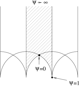
Figure 3: Moduli Space for Elliptic Curve.

4.3 $Z$ is a surface

There is only one possibility, namely $X=E$ is an elliptic fibration over $Z$. We will denote this fibration $\pi:X\to S$. Let $\mathsf{z}\in\mathbf{D}(S)$ correspond to the skyscraper sheaf of a point $s\in S$. Then $\pi^{*}\mathsf{z}\in\mathbf{D}(X)$ corresponds to the structure sheaf of an elliptic fibre $e\subset X$ over $s$.

Let us consider the case where the size of $S$ becomes infinite. According to our rules then, the 2-brane wrapping $e$ should become massless when we hit the discriminant moving from the large radius phase to the phase where the elliptic fibres such as $e$ have collapsed. At first sight this looks peculiar. One does not usually expect a 2-brane wrapped around a 2-torus to become massless for a particular radius of the torus!

Actually we will argue that this indeed happens and that it is when the 2-torus is zero sized that the 2-brane becomes massless. Why T-duality doesn’t interfere with this will become apparent.

As a specific example let $X$ be given by the following equation in ${\mathbb{P}}^{4}_{\{9,6,1,1,1\}}$:

$$x_{1}^{2}+x_{2}^{3}+x_{3}^{18}+x_{4}^{18}+x_{5}^{18}.$$ (82)

This has a quotient singularity which may be resolved with an exceptional divisor ${\mathbb{P}}^{2}$. One may regard $[x_{3},x_{4},x_{5}]$ as homogeneous coordinates on this $S\cong{\mathbb{P}}^{2}$. Fixing a point on $S$ one then has an elliptic fibre $e$ given by a sextic in ${\mathbb{P}}^{2}_{\{3,2,1\}}$. See, for example, [49] for more details about such fibrations.

The moduli space of interest to us regards the area of $e$. This area is infinite for the Calabi–Yau limit point and shrinks down as we approach the other limit point. For a more precise statement let us consider the mirror $\tilde{e}$ of $e$ given by the following equation in ${\mathbb{P}}^{2}_{\{3,2,1\}}$:

$$x_{1}^{2}+x_{2}^{3}+x_{3}^{6}+432^{\frac{1}{6}}\psi x_{1}x_{2}x_{3}.$$ (83)

Varying the size of $e$ is then mirror to varying the complex structure of $\tilde{e}$ by varying $\psi$. Going through the usual story of solving the Picard–Fuchs equation and using the mirror map to map back to the $B+iJ$ plane for $e$ we obtain the shaded region in figure 3.

The result is that for the Calabi–Yau limit point we have $\psi\to\infty$ and thus $J\to\infty$ as expected. For the other limit point $\psi=0$ and $J=\sqrt{3}/2$. The discriminant is given by $\psi=1$ and corresponds to $J=0$, i.e., $e$ has zero area. This is where the 2-branes wrapping $e$ (and all the other D-branes given by $\pi^{*}\mathsf{z}$ for $\mathsf{z}\in\mathbf{D}(S)$) become massless.

So what about T-duality for $e$? Note that the moduli space in figure 3 corresponds to two fundamental regions for the action of $\operatorname{SL}(2,{\mathbb{Z}})$ on the upper-half plane. T-duality should map the point at $\psi=1$ to the point at $\psi=\infty$. It is important to remember however that T-duality does not act only upon $e$ — one must also shift the string dilaton by an amount related to the resulting change in the area of the torus. As such, the point at $\psi=1$ is related to $\psi=\infty$ only with the string coupling shifted off to infinity, implying again that the D-brane mass is zero.

Therefore if we fix the dilaton to be a finite value we cannot use T-duality to relate $\psi=1$ to any large radius torus. This explains why we really do have a massless 2-brane appearing wrapped around a zero-sized torus.

Note also that if we allow the base $S\cong{\mathbb{P}}^{2}$ to have finite size then the T-duality group ceases to exist anyway as in [50].

The fact that there is a T-duality relating $\psi=\infty$ to $\psi=1$ shows that their physics must be similar. In particular $\psi=1$ must be an infinite distance away in the moduli space. Indeed, in many respects the spectrum of stable D-branes at $\psi=1$, coming from the derived category of ${\mathbb{P}}^{2}$, must be similar to the spectrum one would see upon going to a large radius limit. It would be interesting to investigate this in more detail and generality.

4.4 The Exoflop

Finally let us note that not all the walls of the Kähler cone correspond directly to some subspace $E$ collapsing to $Z$. Even so, it appears that we can still fit many, if not all examples into the general EZ language. We illustrate this with an “exoflop”.

Let $X$ be the degree 12 hypersurface in ${\mathbb{P}}^{4}_{\{3,3,3,2,1\}}$. Its mirror, $Y$, then has defining equation

$$a_{0}z_{1}z_{2}z_{3}z_{4}z_{5}+a_{1}z_{1}^{4}+a_{2}z_{2}^{4}+a_{3}z_{3}^{4}+a_{4}z_{4}^{6}+a_{5}z_{5}^{12}+a_{6}z_{4}^{2}z_{5}^{8}+a_{7}z_{4}^{4}z_{5}^{4},$$ (84)

and we may use the following algebraic coordinates on the moduli space of complex structures of $Y$:

$$x=\frac{a_{1}a_{2}a_{3}a_{6}^{2}}{a_{0}^{4}a_{5}},\quad y=\frac{a_{4}a_{6}}{a_{7}^{2}},\quad z=\frac{a_{5}a_{7}}{a_{6}^{2}}.$$ (85)

We have chosen coordinates so that the Kähler cone of $X$ appears naturally as a positive octant in the secondary fan. In particular this means that the 3 rational curves in the moduli space connecting the large radius limit to each of the three neighbouring phase limit points are given by setting $x=y=0$, $x=z=0$ or $y=z=0$ respectively.

The discriminant has two components given by

$$\Delta_{0}=-1-64x+768xz+32768x^{2}z-196608x^{2}z^{2}-4194304x^{3}z^{2}+294912x^{2}yz^{2}\\ +16777216x^{3}(yz^{2}+z^{3})-75497472x^{3}yz^{3}+113246208x^{3}y^{2}z^{4}$$ (86)

and

$$\Delta_{1}=-1+4y+4z-18yz+27y^{2}z^{2}.$$ (87)

The phase transition of interest occurs for the rational curve $C$ for which $y=z=0$. For small $x$ we are in the Calabi–Yau phase. For large $x$ the Calabi–Yau $X$ undergoes an “exoflop” [51]. That is $X$ becomes reducible with one component consisting of a threefold with a singularity. The other component consists of a fibration of a Landau–Ginzburg orbifold theory over a ${\mathbb{P}}^{1}$. These components intersect at a point which is the singularity in the threefold component.

This then is not an EZ transformation. Note however that the discriminant $\Delta_{0}$ intersects $C$ transversely at $(x,y,z)=(-{\textstyle\frac{1}{64}},0,0)$ and so the monodromy within $C$ is exactly given by monodromy around the primary component of the discriminant. Therefore exactly one D-brane becomes massless at the transition point — the D6-brane wrapping $X$. This exoflop transition is equivalent, as far as monodromy is concerned, to an EZ transformation with $X=E$ and $Z$ given by a point.

This is not entirely surprising given the following. Classically one would describe the exoflop wall of the Kähler cone as a wall where $\int_{X}J^{3}=0$. Thus the classical volume of $X$ is going to zero, even though the volume of some surfaces and curves within $X$, as measured by the Kähler form, do not vanish. Since the volume of $X$ vanishes, one should expect the D6-brane to have vanishing mass. The fact that no other D-branes become massless is not obvious.

It would be interesting to show that all phase transitions give rise to monodromies that can be associated with EZ transformations.

References

- [1] M. Kontsevich, Homological Algebra of Mirror Symmetry, in “Proceedings of the International Congress of Mathematicians”, pages 120–139, Birkhäuser, 1995, alg-geom/9411018.
- [2] M. R. Douglas, D-Branes, Categories and =1 Supersymmetry, J. Math. Phys. 42 (2001) 2818–2843, hep-th/0011017.
- [3] C. I. Lazaroiu, Unitarity, D-Brane Dynamics and D-brane Categories, JHEP 12 (2001) 031, hep-th/0102183.
- [4] P. S. Aspinwall and A. E. Lawrence, Derived Categories and Zero-Brane Stability, JHEP 08 (2001) 004, hep-th/0104147.
- [5] D.-E. Diaconescu, Enhanced D-brane Categories from String Field Theory, JHEP 06 (2001) 016, hep-th/0104200.
- [6] M. Kontsevich, 1996, Rutgers Lecture, unpublished.
- [7] R. P. Horja, Hypergeometric Functions and Mirror Symmetry in Toric Varieties, math.AG/9912109.
- [8] P. Horja, Derived Category Automorphisms from Mirror Symmetry, math.AG/0103231.
- [9] M. R. Douglas, B. Fiol, and C. Römelsberger, Stability and BPS Branes, hep-th/0002037.
- [10] M. R. Douglas, B. Fiol, and C. Romelsberger, The Spectrum of BPS Branes on a Noncompact Calabi-Yau, hep-th/0003263.
- [11] M. R. Douglas, Topics in D-geometry, Class. Quant. Grav. 17 (2000) 1057–1070, hep-th/9910170.
- [12] P. S. Aspinwall and M. R. Douglas, D-Brane Stability and Monodromy, JHEP 05 (2002) 031, hep-th/0110071.
- [13] P. S. Aspinwall, A Point’s Point of View of Stringy Geometry, hep-th/0203111.
- [14] A. Strominger, Massless Black Holes and Conifolds in String Theory, Nucl. Phys. B451 (1995) 96–108, hep-th/9504090.
- [15] P. S. Aspinwall and R. L. Karp, Solitons in Seiberg–Witten Theory and the Derived Category, in preparation.
- [16] A. Sen, Tachyon Condensation on the Brane Antibrane System, JHEP 08 (1998) 012, hep-th/9805170.
- [17] J. Distler, H. Jockers, and H. Park, D-Brane Monodromies, Derived Categories and Boundary Linear Sigma Models, hep-th/0206242.
- [18] K. Fukaya, Floer Homology and Mirror Symmetry I, AMS/IP Stud. in Adv. Math. 23 (2001) 15–43.
- [19] P. Seidel, Graded Lagrangian Submanifolds, Bull. Soc. Math. France 128 (2000) 103–149, math.SG/9903049.
- [20] P. Seidel and R. P. Thomas, Braid Groups Actions on Derived Categories of Coherent Sheaves, Duke Math. J. 108 (2001) 37–108, math.AG/0001043.
- [21] T. Bridgeland and A. Maciocia, Fourier-Mukai transforms for Quotient Varieties, math.AG/9811101.
- [22] P. Candelas, X. C. de la Ossa, P. S. Green, and L. Parkes, A Pair of Calabi–Yau Manifolds as an Exactly Soluble Superconformal Theory, Nucl. Phys. B359 (1991) 21–74.
- [23] D. R. Morrison, Geometric Aspects of Mirror Symmetry, in B. Enquist and W. Schmid, editors, “Mathematics Unlimited – 2001 and Beyond”, pages 899–918, Springer-Verlag, 2001, math.AG/0007090.
- [24] P. S. Aspinwall, B. R. Greene, and D. R. Morrison, Measuring Small Distances in Sigma Models, Nucl. Phys. B420 (1994) 184–242, hep-th/9311042.
- [25] D. R. Morrison and M. R. Plesser, Summing the Instantons: Quantum Cohomology and Mirror Symmetry in Toric Varieties, Nucl. Phys. B440 (1995) 279–354, hep-th/9412236.
- [26] V. V. Batyrev, Dual Polyhedra and Mirror Symmetry for Calabi–Yau Hypersurfaces in Toric Varieties, J. Alg. Geom. 3 (1994) 493–535.
- [27] P. S. Aspinwall and B. R. Greene, On the Geometric Interpretation of = 2 Superconformal Theories, Nucl. Phys. B437 (1995) 205–230, hep-th/9409110.
- [28] E. Witten, Phases of Theories in Two Dimensions, Nucl. Phys. B403 (1993) 159–222, hep-th/9301042.
- [29] P. S. Aspinwall, B. R. Greene, and D. R. Morrison, Multiple Mirror Manifolds and Topology Change in String Theory, Phys. Lett. 303B (1993) 249–259.
- [30] P. S. Aspinwall, B. R. Greene, and D. R. Morrison, The Monomial-Divisor Mirror Map, Internat. Math. Res. Notices 1993 319–338, alg-geom/9309007.
- [31] I. M. Gelfand, M. M. Kapranov, and A. V. Zelevinski, Discriminants, Resultants and Multidimensional Determinants, Birkhäuser, 1994.
- [32] B. R. Greene and Y. Kanter, Small Volumes in Compactified String Theory, Nucl. Phys. B497 (1997) 127–145, hep-th/9612181.
- [33] P. Candelas et al., Mirror Symmetry for Two Parameter Models — I, Nucl. Phys. B416 (1994) 481–562.
- [34] P. S. Aspinwall, Some Navigation Rules for D-brane Monodromy, J. Math. Phys. 42 (2001) 5534–5552, hep-th/0102198.
- [35] R. Hartshorne, Algebraic Geometry, Graduate Texts in Mathematics 52, Springer-Verlag, 1977.
- [36] R. Hartshorne, Residues and Duality, Lecture Notes in Math. 20, Spinger-Verlag, 1966.
- [37] D.-E. Diaconescu and J. Gomis, Fractional Branes and Boundary States in Orbifold Theories, JHEP 10 (2000) 001, hep-th/9906242.
- [38] T. Bridgeland and A. Maciocia, Fourier-Mukai Transforms for K3 and Elliptic Fibrations, math.AG/9908022.
- [39] B. Andreas, G. Curio, D. Hernandez Ruiperez, and S.-T. Yau, Fourier–Mukai Transforms and Mirror Symmetry for D-Branes on Elliptic Calabi–Yau, math.AG/0012196.
- [40] A. A. Beilinson, Coherent Sheaves on and Problems in Linear Algebra, Func. Anal. Appl. 12 (1978) 214–216.
- [41] A. A. Beilinson, J. N. Bernstein, and P. Deligne, Faisceaux pervers, Astérisque 100 (1982).
- [42] P. S. Aspinwall, Enhanced Gauge Symmetries and Calabi–Yau Threefolds, Phys. Lett. B371 (1996) 231–237, hep-th/9511171.
- [43] S. Katz, D. R. Morrison, and M. R. Plesser, Enhanced Gauge Symmetry in Type II String Theory, Nucl. Phys. B477 (1996) 105–140, hep-th/9601108.
- [44] E. Witten, Phase Transitions in M-Theory and F-Theory, Nucl. Phys. B471 (1996) 195–216, hep-th/9603150.
- [45] N. Seiberg and E. Witten, Electric - Magnetic Duality, Monopole Condensation, and Confinement in N=2 Supersymmetric Yang-Mills Theory, Nucl. Phys. B426 (1994) 19–52, hep-th/9407087, (erratum-ibid. B430 (1994) 485-486).
- [46] S. Kachru et al., Nonperturbative Results on the Point Particle Limit of N=2 Heterotic String Compactifications, Nucl. Phys. B459 (1996) 537–558, hep-th/9508155.
- [47] S. Katz, P. Mayr, and C. Vafa, Mirror Symmetry and Exact Solution of 4D N = 2 Gauge Theories. I, Adv. Theor. Math. Phys. 1 (1998) 53–114, hep-th/9706110.
- [48] A. Klemm et al., Self-Dual Strings and N=2 Supersymmetric Field Theory, Nucl. Phys. B477 (1996) 746–766, hep-th/9604034.
- [49] C. Vafa and E. Witten, Dual String Pairs With and Supersymmetry in Four Dimensions, in “S-Duality and Mirror Symmetry”, Nucl. Phys. (Proc. Suppl.) B46, pages 225–247, North Holland, 1996, hep-th/9507050.
- [50] P. S. Aspinwall and M. R. Plesser, T-Duality Can Fail, J. High Energy Phys. 08 (1999) 001, hep-th/9905036.
- [51] P. S. Aspinwall, B. R. Greene, and D. R. Morrison, Calabi–Yau Moduli Space, Mirror Manifolds and Spacetime Topology Change in String Theory, Nucl. Phys. B416 (1994) 414–480.