MCTP-02-47
Interacting Quantum Field Theory
in de Sitter Vacua

We discuss interacting quantum field theory in de Sitter space and argue that the Mottola-Allen vacuum ambiguity is an artifact of free field theory. The nature of the nonthermality of the MA-vacua is also clarified. We propose analyticity of correlation functions as a fundamental requirement of quantum field theory in curved spacetimes. In de Sitter space, this principle determines the vacuum unambiguously and facilitates the systematic development of perturbation theory.

1 Introduction

The quantum theory of de Sitter space is important because it plays a central role in cosmology, particularly in the generation of cosmic structure from inflation and in the puzzles surrounding the cosmological constant. More generally, de Sitter space is useful for testing theoretical ideas because, as a maximally symmetric space, it is tightly constrained. Eventually, we want to understand the full quantum gravity of de Sitter space, but many interesting questions appear already at the level of quantum field theory (QFT) in a fixed de Sitter background. In this paper we study the vacuum structure of the theory and develop the features of interacting QFT needed for this purpose.

The starting point of QFT in any background is a mode expansion

$$\phi(X)=\sum_{n}[a_{n}u_{n}(X)+a_{n}^{\dagger}u_{n}^{*}(X)]~{},$$ (1)

and the corresponding specification of the vacuum

$$a_{n}|{\rm vac}\rangle=0~{}.$$ (2)

The modes $u_{n}$ must be chosen so that the corresponding vacuum respects the symmetries of the theory. In Minkowski space this principle determines the modes completely and, accordingly, there is a unique Poincaré invariant vacuum. In curved spacetime, symmetries do not in general determine the vacuum state completely. Indeed, in de Sitter space, symmetries identify the vacuum only modulo a two parameter ambiguity, corresponding to a family of distinct de Sitter invariant vacua. The existence of this ambiguity was first emphasized by Mottola[1] and Allen[2].

One vacuum is almost universally taken as the starting point for QFT in de Sitter space. We will refer to this vacuum as the “Euclidean vacuum” and reserve the term “MA-vacua” for the alternative, nonstandard vacua. The Euclidean vacuum is singled out by several features:

• The correlation functions can be obtained by continuation from the Euclidean de Sitter space, i.e. a sphere. This is the origin of the terminology we employ.

• It coincides with the adiabatic vacuum in the FRW coordinates customarily employed in cosmology. This facilitates a consistent particle interpretation of the theory. In cosmology the Euclidean vacuum is often referred to as the Bunch-Davies vacuum[3].

• The correlations of the field are experienced as precisely thermal by an Unruh detector (a comoving detector linearly coupled to the quantum field).

• The $2$-point correlation functions reduce to the standard Minkowski propagators when the de Sitter radius is taken to infinity.

These properties are desirable both technically and conceptually, but they do not by themselves identify the Euclidean vacuum as the “right” vacuum. It could be that the MA-vacua simply have different properties, and that the question of which vacuum is appropriate depends on additional physical input such as boundary conditions, or even observational data. This is the point of view taken in much recent work[4, 5, 6, 7, 8, 9].

Previous discussions have been at the level of free field theory in fixed background. In most contexts, such as effective field theory, what we are really interested in is the weakly interacting theory; so it is important that higher order interactions can be included, at least in principle. In this paper we argue that this is possible only for the Euclidean vacuum. The problems we encounter in the general case are particularly sharp for the loop amplitudes. For these the issue is not that amplitudes take values we deem physically unreasonable; rather, they are ill-defined in the MA-vacua, a much worse problem. Tree level amplitudes are also problematic even though they are mathematically well-defined: they have unusual, and most likely physically unacceptable, singularities related to antipodal events which, as we discuss, cannot be hidden behind an event horizon. We conclude that the MA-vacua are artifacts of the free field limit. Of course, we cannot actually prove that no definition of the MA-vacua exists at the interacting level. What we argue is that it is known how to include interactions in the Euclidean vacuum, and, whenever the propagator is not the boundary value of an analytic function, as in these MA-vacua, this prescription does not generalize. Thus, at the very least, more work is needed to establish the viability of the MA-vacua.

Relativistic QFT is a tight structure. In addition to symmetries, the interacting theory is constrained by analyticity properties. The principle we need is

• Correlation functions are boundary values of analytical functions (in the sense of distributions).

This principle singles out the Euclidean vacuum. Following Bros et al.[10, 11, 12, 13], it allows one to construct an interacting theory for de Sitter space that closely mimics QFT in Minkowski space. For example, it ensures the Källén-Lehman representation for the two-point Green’s function with a positive spectral density. The non-existence of an S-matrix, a major confusion clouding the quantum theory of de Sitter space, can be circumvented, at least for our purposes, by considering correlation functions directly. It is the correlation functions that are observables, measured by Unruh detectors, and it is the correlation functions that satisfy strong analyticity properties. These may be important lessons for formulating the quantum theory of de Sitter space.

One of the motivations for studying the MA-vacua is their possible applications to cosmology. According to the inflationary paradigm, all structure in the universe ultimately originated from the fluctuations of a scalar field in a de Sitter background. It has been proposed that physics at extremely high “trans-Planckian” energies determines which vacuum is appropriate for this scalar field and thus, using the MA-vacua as interlocutor, the cosmic structure could contain data pertaining to such energies[7, 8]. In this regard our results are unfortunately negative: they indicate that this possibility is illusory, at least in its simplest form.

The remainder of the paper is organized as follows. In section 2 we review the classical de Sitter geometry, QFT in the de Sitter background, and the MA-vacua in the free theory. In section 3 we first discuss some general features of interacting QFT in curved spacetimes and singularities of amplitudes. Then we exhibit the problems with the MA-vacua, considering in turn tree level amplitudes and loops. In section 4 we discuss the nature of the non-thermality of the MA-vacua, and examine some of their difficulties from this point of view. Finally, in section 5, we discuss implications of our results as well as future research directions.

2 Quantum Field Theory in de Sitter Space

The purpose of this section is to review properties of the de Sitter geometry and QFT in the de Sitter background with special emphasis on the MA-vacua. The primary reference is [2].

2.1 Classical Geometry

The d-dimensional de Sitter space ($dS_{d}$) can be represented as the hyperboloid

$$X^{2}=X^{2}_{0}-\vec{X}^{2}=-l^{2}~{},$$ (3)

in $d+1$ dimensional Minkowski space

$$X^{M}=(X^{0},X^{1},\ldots,X^{d})~{},$$ (4)

with signature $(+,-,\ldots,-)$. De Sitter space is maximally symmetric with isometry group $SO(1,d-1)$; and it is a solution to pure gravity with cosmological constant $\Lambda={1\over 2}(d-1)(d-2)l^{-2}~{}.$ We take $l^{2}=1$ in the following.

The $SO(1,d)$ invariant distance between different points $X$ and $Y$ is

$$Z=-X\cdot Y=\vec{X}\cdot\vec{Y}-X^{0}Y^{0}~{}.$$ (5)

The $X$ and $Y$ are timelike separated if $Z>1$ and spacelike separated for $Z<1$. For $Z<-1,$ no geodesic exists that join $X$ and $Y$, even though the spacetime is geodesically complete.

The constraint equation defining de Sitter space (3) is invariant under $X\to-X$; so for any $X$ in de Sitter space, the antipodal event $X_{A}=-X$ is also in de Sitter space. The invariant distance between an event and its antipodal is $Z=-X\cdot X_{A}=-1$. This means their future (past) lightcones cross only in the asymptotic future (past). Antipodal events cannot communicate; they never have, and they never will.

The embedding coordinates $X^{M}$, and the invariant distance $Z$, are the most convenient for our purposes. Various explicit coordinates, solving the embedding relations, are more familiar in other contexts. For their relation to embedding coordinates, see the recent review [4].

The invariant distance $Z=Z(X,Y)$ is symmetric in its two arguments; so it does not distinguish between the future and past lightcone. For such purposes we introduce ${\,\rm Sgn}(X,Y)$; it is equal to $+1~{}(-1)$ when $X$ is in or on the forward (backward) lightcone of $Y$, and equal to $0$ for spacelike directions. The ${\,\rm Sgn}(X,Y)$ is invariant under de Sitter symmetries continuously connected to the identity, but it changes sign under time reversal.

2.2 Quantum Fields in de Sitter Space

We want to study quantum field theory in the de Sitter background. The simplest example is a free scalar field

$${\cal L}={1\over 2}[\partial_{\mu}\phi\partial^{\mu}\phi-m^{2}\phi^{2}-\xi{\cal R}\phi^{2}]~{}.$$ (6)

Since the scalar curvature ${\cal R}={\rm const}=d(d-1)$ in de Sitter space, we can absorb the coupling $\xi$ into an effective mass $\tilde{m}^{2}=m^{2}+\xi{\cal R}$ and henceforth consider minimal coupling $\xi=0$ without loss of generality. The starting point for quantization of the field theory is a complete set $\{u_{n}\}$ of properly normalized solutions to the Klein-Gordon equation. The quantum field is expanded in these modes as in (1), and the vacuum is defined as in (2).

An important observable is the two point Wightman function

$$G^{W}(X,Y)=\langle{\rm vac}|\phi(X)\phi(Y)|{\rm vac}\rangle~{}.$$ (7)

The Wightman function is essentially the response function of an Unruh detector, i.e. a detector carried by a comoving observer; so it is indeed a physical observable, at least for timelike separated intervals. In the free theory, it determines all other correlators, and thus the full theory. It is convenient to split the Wightman function into symmetric and anti-symmetric parts

$$G^{W}(X,Y)={1\over 2}\left[G^{(1)}(X,Y)+iD(X,Y)\right]~{},$$ (8)

known as the Hadamard function and the commutator function, respectively. They have the mode expansions

$$G^{(1)}(X,Y)=\langle{\rm vac}|\{\phi(X),\phi(Y)\}|{\rm vac}\rangle=\sum_{n}[u_{n}(X)u^{*}_{n}(Y)+u_{n}^{*}(X)u_{n}(Y)]~{},$$ (9)

and

$$iD(X,Y)=\langle{\rm vac}|[\phi(X),\phi(Y)]|{\rm vac}\rangle=\sum_{n}[u_{n}(X)u^{*}_{n}(Y)-u_{n}^{*}(X)u_{n}(Y)]~{}.$$ (10)

As usual, the Feynman propagator is the time-ordered Green’s function

$$iG^{F}(X,Y)=\langle{\rm vac}|T[\phi(X)\phi(Y)]|{\rm vac}\rangle={1\over 2}\left[G^{(1)}(X,Y)+i{\,\rm Sgn}(X,Y)D(X,Y)\right]~{}.$$ (11)

2.3 The Euclidean Vacuum

In the Euclidean vacuum, the modes $\{u_{n}\}$ are chosen as the regular solutions of the Klein-Gordon equation on Euclidean de Sitter space, i.e. the sphere. The correlation functions can then be computed from (9- 10), by carrying out the mode sums and then continuing back to Lorentzian signature. This procedure gives the generic two-point function

$$f(Z)\equiv C_{d,\nu}F(h_{+},h_{-},{d\over 2},{1+Z\over 2})~{},$$ (12)

where $F$ is the hypergeometric function, the weights are $h_{\pm}={d-1\over 2}\pm i\nu$, and

$$\nu = \sqrt{m^{2}-\left({d-1\over 2}\right)^{2}}~{},$$ (13)

$$C_{d,\nu} = {\Gamma(h_{+})\Gamma(h_{-})\over(4\pi)^{d/2}\Gamma({d\over 2})}~{}.$$ (14)

The function (12) is real in the spacelike region $Z<1$, and it has a pole on the lightcone $Z=1$, which extends to a cut for lightlike $Z>1$ (except when the $h_{\pm}$ are real and integral.) It is analytic in the complex plane away from the cut. The normalization constant $C_{d,\nu}$ is set by the condition that the pole at $Z=1$ has unit strength, as it must be after the canonical commutation relations have been properly imposed.

The various correlation functions are distinguished by the prescription along the cut. The Hadamard function is real and so defined by taking the average across the cut

$$G^{(1)}_{0}=f(Z+i\epsilon)+f(Z-i\epsilon)=2~{}{\rm Re}f(Z)~{}.$$ (15)

The Wightman function has a definite ordering of the fields; so its expansion involves the modes $u_{n}(X)$, but the complex conjugate modes $u^{*}_{n}(Y)$. The prescription regulating the corresponding infinite sum is

$$G^{W}_{0}=f(Z-i\epsilon{\,\rm Sgn}(X,Y))~{}.$$ (16)

The Wightman function depends only on the invariant distance $Z=-X\cdot Y$, except for the allowance for time-ordering. This property assures de Sitter invariance of the vacuum. The commutator function is determined from (8) as

$$D_{0}=2{\rm Im}~{}G^{W}_{0}=2{\rm Im}~{}f(Z-i\epsilon{\,\rm Sgn}(X,Y))~{}.$$ (17)

This expression vanishes for spacelike separations $Z<1$, as it should to comply with microcausality. Comparing (8) and (11), we find the Feynman propagator

$$iG^{F}_{0}=f(Z-i\epsilon)~{}.$$ (18)

The subscript $0$ on each of these correlation functions indicates the Euclidean vacuum.

The index $\nu$ (13) is real for $m^{2}>({d-1\over 2})^{2}$ and purely imaginary for $m^{2}<({d-1\over 2})^{2}$. The nature of the corresponding wave functions differ qualitatively: the “large mass” case looks wavy, whereas the “small mass” wave functions are exponentially damped. The corresponding representations of the de Sitter group are known as the principal series and the complementary series, respectively.

The formula (12) for the function $f(Z)$ simplifies in the conformally coupled massless case, equivalent in de Sitter space to the effective mass $m^{2}=d(d-2)/4$. This mass is in the range corresponding to the complementary series. The $d=4$ example

$$f(Z)={1\over 8\pi^{2}}~{}{1\over Z-1}~{},$$ (19)

just has a simple pole, rather than a cut. The correlation functions (15,16,18) then simplify correspondingly and (17) gives

$$D_{0}(X,Y)={1\over 4\pi}~{}{\,\rm Sgn}(X,Y)~{}\delta(Z-1)~{}.$$ (20)

These expressions are much more transparent to work with than the generic ones, involving the hypergeometric functions. We will therefore use this special case in explicit computations.

2.4 The MA-vacua

Alternative choices of the modes $\{u_{n}\}$ give rise to different vacua. The most general option is given by the Bogoliubov transformation

$${\tilde{u}}_{n}(X)=\sum_{n^{\prime}}\left[A^{*}_{nn^{\prime}}u_{n^{\prime}}(X)-B^{*}_{nn^{\prime}}u^{*}_{n^{\prime}}(X)\right]~{},$$ (21)

of the Euclidean modes. The commutation relations of the QFT impose the normalization conditions

$$AA^{\dagger}-BB^{\dagger}=I~{},$$ (22)

on the matrices $A$, $B$; and de Sitter invariance requires each to be proportional to the identity matrix $I$. The Bogoliubov transform (21) therefore takes the form

$${\tilde{u}}_{n}(X)=\cosh\alpha~{}u_{n}(X)+\sinh\alpha~{}e^{i\beta}~{}u_{n}^{*}(X)~{},$$ (23)

up to an irrelevant overall phase. With the choice of basis in which $u_{n}^{*}(X)=u_{n}(X_{A}),$ the corresponding correlation functions can be expressed in terms of the Euclidean ones as

$$G^{(1)}_{\alpha,\beta}(X,Y)=\cosh 2\alpha~{}G^{(1)}_{0}(Z)+\sinh 2\alpha~{}\left[\cos\beta G^{(1)}(-Z)-\sin\beta D_{0}({X_{A}},Y)\right]~{},$$ (24)

and

$$D_{\alpha,\beta}(X,Y)=D_{0}(X,Y)~{}.$$ (25)

So the vacua parameterized by $(\alpha,\beta)$ are indeed invariant under proper de Sitter transformations. These are the MA-vacua.

The Euclidean commutator function $D_{0}$ changes sign under time-reversal $T(X_{0},\vec{X})=(-X_{0},\vec{X})$ so the nonstandard Hadamard functions transform as

$$G^{(1)}_{\alpha,\beta}(T(X),T(Y))=G^{(1)}_{\alpha,-\beta}(X,Y)~{}.$$ (26)

This means the MA-vacua violate CPT invariance for $\beta\neq 0$.

The Feynman propagators in the MA-vacua are (for Z real)

$$G^{F}_{\alpha,\beta}(Z)=\cosh^{2}\alpha\,G_{0}^{F}(Z)-\sinh^{2}\alpha(G_{0}^{F}(Z))^{*}+\sinh 2\alpha\left({1\over 2}e^{i\beta}G_{0}^{F}(-Z)+{\rm c.c.}\right)$$ (27)

and similarly for the Wightman function $G^{W}_{\alpha,\beta}(Z)$. In the conformally invariant case (19)

$$iG^{F}_{\alpha,0}(X,Y)={1\over 8\pi^{2}}[\cosh^{2}\alpha{1\over Z-1-i\epsilon}+\sinh^{2}\alpha{1\over Z-1+i\epsilon}+\sinh 2\alpha{1\over Z+1}]~{},$$ (28)

for $\beta=0$. This expression has several noteworthy features

• The strength of the pole along the lightcone $Z=1$, and thus the ultraviolet divergences, are larger than they would be in flat space. The renormalization program can therefore not rely on the flat space limit to determine the appropriate counterterms.

• There is a pole along the lightcone $Z=-1$ emanating from the antipodal event. Such correlations will appear as acausal effects in some processes (see section 3.2) .

• The two terms having poles along the light-cone $Z=1$ have opposite $i\epsilon$ prescriptions. Similarly, the pole along the lightcone of the antipodal event $Z=-1$ is understood as a principal value, i.e. the average of the two $i\epsilon$ prescriptions with opposite sign. This structure will render loop amplitudes ill-defined (see section 3.3).

These features are not merely unfamiliar, they prevent a definition of the theory at the interacting level.

The MA-vacua can formally be represented as squeezed states in the Euclidean vacuum

$$|\alpha,\beta\rangle={\cal N}~{}\exp\left(-{1\over 2}\sum_{n}[\alpha e^{-i\beta}(a_{n}^{\dagger})^{2}-{\rm c.c.}]\right)|0,0\rangle~{}.$$ (29)

According to this representation the MA-vacua can be interpreted as minimal uncertainty states with the field in opposite ends of the universe correlated precisely at the quantum level. Of course, these squeezed states are not normalizable and therefore the $|\alpha,\beta\rangle$ are actually not elements in the Hilbert space of the Euclidean vacuum $|0,0\rangle$. That is one reason why the MA-vacua really are new vacua, and not just a special class of states.

3 Interacting Quantum Fields

In this section we first discuss the general issues of observables in de Sitter space, Feynman rules in curved spacetimes, and the singularities of QFT amplitudes. We then apply these remarks to the MA-vacua, discussing in turn the tree amplitudes and loops. The section ends with comments on axiomatic QFT in the Euclidean vacuum.

3.1 Fundamentals

One question that arises in curved spacetimes is what can be observed. In general, there are no asymptotically-flat regions in which to define in- and out-states. Thus, there is no well-defined S-matrix, although in de Sitter space, there have been discussions of meta-amplitudes[15, 6] for transitions between states defined on the past null infinity (${\cal I}^{-}$) and the future null infinity (${\cal I}^{+}$). For our purposes, it is sufficient to imagine observers carrying calibrated detectors, idealized as Unruh detectors, that can be used to probe interactions with the field on their (timelike) trajectories. The corresponding “detector response function” probes the two-point correlation function (or Wightman function) of the field. (This has been reviewed in refs [16, 4, 5].) Going beyond the usual linear response analysis, it should be possible to measure higher point correlators as well. Moreover, further correlations can be accessed by introducing several detectors or independent observers. We will assume that all Wightman functions are in principle observable, at least for points separated by timelike geodesics.

In some applications, the arguments of the correlation functions should be restricted to take values within a given static patch. For example, the complementarity principle can be taken to assert that, in the complete quantum theory of gravity, the full set of correlators, restricted in this way, form a complete set of observables[17]. This is consistent with our interpretation of correlators, motivated by effective field theory. Indeed, “complementarity” precisely states that the fundamental, holographic view of observables is consistent with the low energy, local interpretation of physics. In the present context the latter is more appropriate.

The next question is how to get the Feynman rules for calculating correlation functions perturbatively. In fact, moving beyond free field theory to interacting field theories in a fixed, curved background is fairly straightforward. Formally, we may define the Feynman rules for perturbation theory in the same way that it is done in Minkowski space via the Feynman path integral (FPI).

$$e^{iW[J]}=e^{i\int dx\sqrt{g}{\cal L}_{I}(-i\frac{\delta}{\delta J})}e^{iW_{f}[J]}~{},$$ (30)

where $W[J]$ is the generating functional of connected Green’s functions, and ${\cal L}_{I}(\phi)$ is the interaction Lagrangian density (assumed to be nonderivative). $W_{f}[J]$ is the free field generating functional given by

$$W_{f}[J]={1\over 2}\int dx\sqrt{g(x)}dy\sqrt{g(y)}J(x)G^{F}_{\alpha,\beta}(x,y)J(y)~{}.$$ (31)

In Minkowski space, the FPI underlying this expression is normally defined by its Euclidean counterpart[18]. Since, in the MA-vacua, the propagators are not analytic and do not permit a Wick rotation, we cannot employ such a convention here but instead wish to work directly in Lorentzian signature. A common prescription is simply to replace $m^{2}$ by $m^{2}-i\epsilon$ to achieve convergence of the FPI. Alternatively, the expressions (30) and (31) make sense formally without any reference to functional integration. Thus, the coordinate space Feynman rules in general curved spacetime have the same general form as in flat space but with a modified propagator and with insertion of the appropriate factors of the background metric. These observations apply to any quantum field theory (QFT) in curved spacetime, not just to de Sitter space.

According to these rules Feynman amplitudes are written as integrals over various products of propagators as determined by the vertices. We are interested in the nature of singularities of such expressions. Propagators are distributions rather than functions, i.e., they become singular for certain values of their arguments. Generally, $n$-point correlation functions, in the physical region, are also distributions rather than real functions. Distributions make sense as linear functionals when integrated over certain test functions. However, it is by no means obvious that Feynman amplitudes, involving products of propagators and consequently products of distributions, are well-defined.

For the usual vacuum in Minkowski space, the situation is well-understood [20]. All Wightman functions are boundary value distributions of analytic functions. All Feynman integrals can, by a Wick rotation to Euclidean signature, be written in such a way that the integrands have no singularities at all. Renormalization may be carried out for Euclidean signature, so the renormalized $n$-point functions are well-defined and nonsingular for Euclidean signature. Upon analytic continuation back to Minkowski space, singularities may be encountered, but only when certain “causal, on-shell” conditions are satisfied. The upshot is that all renormalized $n$-point functions are well- defined functions in the physical region for Lorentzian signature, except for singularities that correspond to physically allowed processes.

It seems that this program may also be extended to de Sitter space in the Euclidean vacuum[10, 11, 12, 13]. However, in the MA-vacua, the propagators are very different distributions whose singularities prevent analytic continuation. As a result, it is not at all clear that a sensible perturbation expansion can be associated with the formal Feynman rules. One must address old questions anew, such as, when do the singularities of integrands of Feynman amplitudes correspond to singularities of the integrals?

3.2 Tree Amplitudes

We first show that, at tree level, all Feynman amplitudes are in fact mathematically well-defined. Indeed, consider a particular perturbative contribution to an $n$-point function $G_{\alpha,\beta}^{(n)}(x_{1},x_{2},\ldots,x_{n})$ associated with the time-ordered product of fields. Propagator singularities correspond to hypersurfaces in the multidimensional spacetime of the integrand of the Feynman amplitude. For any Feynman diagram, one may choose values for the external points so that the external propagators are nonsingular at points of integration where internal propagators diverge. So one need not worry about coincident singularities involving external legs; it is only the truncated $n$-point functions that could cause problems. Tree diagrams are special inasmuch as the truncated amplitude involves no internal integrations and, for generic external points, there are no propagators having coincident singularities (such as squares of propagators as will appear in loops.) Therefore, the truncated diagram is well-defined except for special values of the external points. When one reattaches external legs, the new integrations will not produce coincident singularites except possibly for special values of the external points. One need only show that the full Green’s function is independent of the order in which the external legs are reattached, which is the case. In other words, the definition of propagators as linear functionals suffices to define tree diagrams so, in tree approximation, the $n$-point function is well-defined for some range of external points.

On the other hand, an amplitude thus defined clearly has singularities for particular external points and, in order to have a properly defined theory, those singularities must have a sensible physical interpretation. In the MA-vacua, the singularities in the propagators associated with the antipodal point give rise to seemingly unphysical singularities in amplitudes which are a serious cause of concern. A possible resolution of this problem is that the antipodal points are somehow “hidden” behind a horizon but, as we show next, in the interacting theory these singularities cannot be so easily hidden.

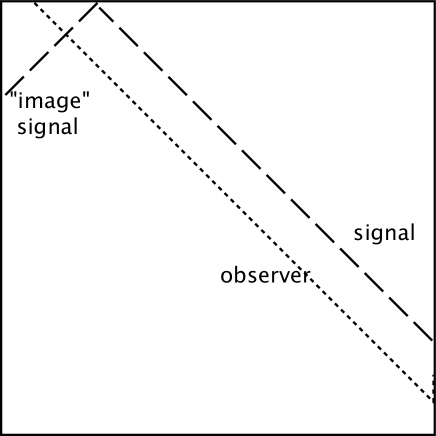
Figure 1: Causal relations to the antipodal point.

Consider generating a signal at the south pole, propagating towards the north pole, and a corresponding “image” disturbance from the antipodal point propagating from the north pole (see fig. 1.) The respective lightcones meet only in the asymptotic future, at ${\cal I}^{+},$ but this does not mean the “image” is unobservable. Any observer sent off (at the speed of light) prior to generating the signal will experience the “image”. Alternatively, when gravitational back-reaction is taken into account, the causal diagram of de Sitter space will become slightly “taller”[19], and so the signal and its “image” can meet. These simple examples suggest that the antipodal singularities are in fact a cause for concern in the interacting theory.

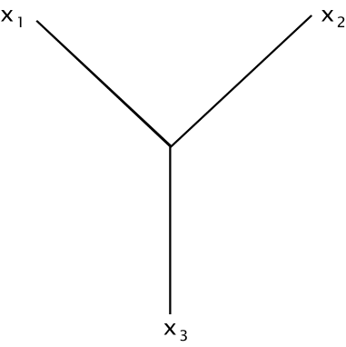
Figure 2: Simple tree diagram.

To verify this expectation in perturbation theory, consider the simple case of a $\lambda\phi^{3}$ interaction and the three-point function (fig. 2) with amplitude

$$G^{(3)}(x_{1},x_{2},x_{3})=-\lambda\int dy\sqrt{g(y)}G^{F}_{\alpha,\beta}(x_{1},y)G^{F}_{\alpha,\beta}(x_{2},y)G^{F}_{\alpha,\beta}(x_{3},y)~{}.$$ (32)

The integration runs over all of de Sitter space. Each of the propagator factors $G^{F}_{\alpha,\beta}(x_{i},y)$ is singular when $y$ is on the lightcone of the corresponding point $x_{i}$ or of its antipode $x_{iA}.$ Consider the external points $x_{i}$ situated as in the Penrose diagram in fig. 3

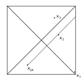
Figure 3: Penrose diagram for three points.

The event $x_{1}$ is on (or near) ${\cal I}^{-},$ and the point $x_{3}$ is within the causal future of $x_{1},$ but near the lightcone and just outside the causal diamond. Thus, its antipode, $x_{3A}$ lies just outside the causal future of $x_{1},$ so that $Z(x_{3A},x_{1})<-1.$ Nevertheless, the point of integration $y$ may lie on the future lightcone of $x_{3A}$ while within the causal diamond of $x_{1}.$ Moreover, singularities of the propagators coincide if $x_{2}$ also lies on the lightcone of $x_{3A}$. In this case the integral, and thus the amplitude, will be singular. Since $x_{1}$, $x_{2}$, $x_{3}$ can be placed on a nowhere spacelike trajectory, we find it difficult to believe that this (singular) correlation would not be not observable. Moreover, being a tree diagram, the effect discussed here is essentially a property of the classical theory. We also note these are not short-distance singularities but are associated with all points on the lightcones, no matter how distant from the apex.

These considerations do not prove that the singularities of tree-amplitudes, however unintuitive and nonlocal, are absolutely impermissible; but such singularities certainly would lead to strange events and traumatic experiences. Their existence raise serious questions about the interpretation, and possibly even the viability, of the MA-vacua.

That tree diagrams can be defined is helpful also in understanding free field theory. One could of course regard the mass term as a two-point interaction vertex and build up the full propagator by summing up this interaction. For consistency, one ought to get the same answer as in (27). The fact that tree amplitudes are well-defined ensures that this can be done, and the result will be unambiguous. Unfortunately, this conclusion does not extend to loop amplitudes, to which we now turn.

3.3 Loop Amplitudes

The analysis of higher order corrections, involving loop amplitudes, is more complicated but also more bedamning. When the propagators are boundary values of analytic functions, as in the Euclidean vacuum in Minkowski or de Sitter space, the general conditions under which a singularity of the integrand actually results in a singularity of the integral have been thoroughly analyzed and are reviewed, for example, in [20]. In Minkowski space, the singularities are generally discussed in momentum space, where they have been codified by the Landau rules[21], or by a related prescription, Cutkosky’s “cutting rules”[22] for putting internal particles on-mass-shell. Although this methodology is not available for theories in curved spacetime, the same sort of analysis can be applied to a coordinate space formulation. We shall illustrate this in the case of the self-energy diagram below, but first we shall try to provide an overview of the issues.

In general, a singularity of the integrand is not a singularity of the integral if the integrand is sufficiently analytic in a neighborhood of the singularity so that the path of integration can be deformed and moved away from the singularity. In the Euclidean vacuum where the propagators are boundary values of analytic functions, singularities of the integrand do not generally yield singularities of the integral because, loosely speaking, the propagators involve a consistent prescription with all masses having infinitesimal negative imaginary parts (the familiar $-i\epsilon$ prescription). The most common exception that produces a singularity of the integral, and the one of particular interest in the present context, is when the contour is “pinched” between singularities of the integrand that coalesce from opposite sides of the integration contour, preventing its deformation away from the singularities. Normally, the pinch only occurs when more than one propagator are simultaneously singular. Even in the Euclidean vacuum, since propagators are distributions rather than functions, it is by no means obvious that products of singularities make sense. Once again, analyticity comes to the rescue, because for Euclidean signature, the integrands are nonsingular, and, once again, it is possible to show that the integrals in the physical region are boundary values of analytic functions. However, for the MA-vacua, where the propagators do not have such analyticity, this pinching occurs for each individual propagator. When singularities of different propagators coincide, it seems to be doubtful that a well-defined determination of the Feynman integral can be made.

We shall show next that even the simplest of loop diagrams is not well-defined for the MA-vacua. The self-energy diagram of fig. 4 is one of the most elementary loop diagrams occuring in perturbation theory. The associated expression is

$$-\lambda\int dx\sqrt{g(x)}dy\sqrt{g(y)}G_{\alpha,\beta}^{F}(x_{1},x)G_{\alpha,\beta}^{F}(x,y)^{2}G_{\alpha,\beta}^{F}(y,x_{2})~{},$$ (33)

involving the square of the internal propagator. Although the self-energy requires renormalization, we shall assume that appropriate counterterms have been included.

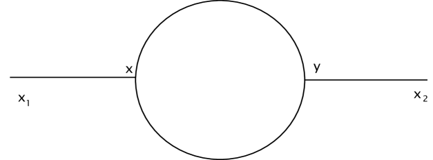
Figure 4: Self-energy diagram.

In Minkowski space, the loop does not contribute a singularity to the self-energy unless the pair $(x,y)$ are such that the particles in the loop are real, that is, on-mass-shell, propagating forward in time[23]. Otherwise, because of the analyticity of the Feynman propagators, the potential singularities of the integrand can be avoided. Another way to state the same result is that the Green’s functions are all nonsingular for Euclidean signature, and the only singularities encountered in analytic continuation to the physical region arise for classically realizable processes. In de Sitter space, the propagator is not analytic in the MA-vacua but only in the Euclidean vacuum. Moreover, the propagator is a distribution whose square is ill-defined, i.e., the square of principal values and delta-functions are not defined. We simply do not know how to define this integral. It seems incumbent upon those who propose to work in these non-standard vacua to explain the rules of calculation and their interpretation.

Although our arguments are generic, we shall illustrate the problems in the specific case of the massless, conformally coupled scalar, for which the various two-point functions reduce to poles at $Z=\pm 1$, their principal values, or imaginary parts. For that case, the discussion is not obscured by the complications of dealing with hypergeometric functions.

Before discussing the de Sitter case, let us first remind ourselves of the situation in flat space. The one-particle-irreducible (1PI) self-energy

$$\Sigma(x,y)\propto\left[\frac{1}{(x-y)^{2}-i\epsilon}\right]^{2}.$$ (34)

This highly singular expression is manageable inside integrals such as (33), because its singularities lie on the same side of the integration contour. If we imagine performing the integration over $x^{0}$ or $y^{0}$, then we have $x^{0}-y^{0}=\pm(|\vec{x}-\vec{y}|+i\epsilon$), as depicted by the crosses in fig. 5.

Figure 5: Pinched singularities.

This does not produce a singularity as $\epsilon\to 0$ unless it occurs in an integral in which another singularity prevents deforming the path of integration. The full expression, (33), involves

$$G^{F}(x_{1},x_{2})\propto\int dxdy\frac{1}{(x_{1}-x)^{2}-i\epsilon}\Sigma(x,y)\frac{1}{(y-x_{2})^{2}-i\epsilon}.$$ (35)

Since the propagators for the external legs depend on the external points, their singularities will not in general coincide with those of $\Sigma(x,y).$ Thus, it is only special values of $(x_{1}-x_{2})$ that produce a singular integral. In this case, by the Coleman-Norton theorem[23], these occur only when $(x_{1}-x_{2})$ is a null vector, and $x$ and $y$ are proportional to $(x_{1}-x_{2}),$ so that $(x_{1}-x)$ and $(y-x_{2})$ are also null.

Now consider the corresponding situation in de Sitter space in an MA vacuum, with

$$\Sigma(x,y)\propto\left(G_{\alpha,\beta}^{F}\right)^{2},$$ (36)

where the propagator $G_{\alpha,\beta}^{F}$ is given in (27). This square involves a great many terms and is rather complicated. We shall simplify the discussion in two inessential ways: we restrict our attention to the CP-invariant vacua, $\beta=0,$ and we focus on the conformally massless case (28). Then, the 1PI-self-energy involves terms of various sorts. From the terms with singularities at $Z=1,$ we get a cross-term of the form

$$\frac{\sinh^{\alpha}\cosh^{2}\alpha}{(Z(x,y)-1-i\epsilon)(Z(x,y)-1+i\epsilon)},$$ (37)

where

$$Z(x,y)-1={1\over 2}(X-Y)^{2}=\frac{(\eta_{x}-\eta_{y})^{2}-(\vec{x}-\vec{y})^{2}}{2\eta_{x}\eta_{y}}.$$ (38)

The first expression involves the embedding coordinates associated with the points $x$ and $y,$ while, in the second form, we have represented this factor in planar coordinates[4], since the denominators then look the same as in flat space. (In planar coordinates, the metric is conformally flat, taking the form

$$ds^{2}=\frac{1}{\eta^{2}}\left(d\eta^{2}-d\vec{x}^{2}\right).$$

Although the coordinates are singular at $\eta=0,$ this is of no consequence for the discussion of the singularities of the self-energy.) Because the denominators in (37) involve opposite signs of $i\epsilon,$ there are now complementary singularities denoted by the circles in fig. 5, so the singularity at $Z=1$ pinches the contour regardless of the values of the external points. Even if such a peculiar singularity were somehow physically acceptable, what is the value of an integral in which it appears? To be the principal value, there would have to be a factor of $Z-1$ in the numerator; to be a delta-function, there would have to be a factor of $\epsilon$ in the numerator. As it is, it lacks definition, and the self-energy is ill-defined. This cannot be cured by local counterterms in the Lagrangian; it happens everywhere along the lightcone. A similar thing is true of the contribution of the antipodal singularity at $Z=-1.$ It is initially defined as the principal value in (28), so its square is ill-defined for the same reason. The CPT-noninvariant case, $\beta\neq 0,$ introduces further conundrums.

The only case that avoids such problems is the Euclidean vacuum, $\alpha=\beta=0,$ for which there is a consistent sign to the $i\epsilon$ assignment, just as in Minkowski space. The discussion of singularities carries over to the de Sitter case, complicated only by having just a coordinate space rather than a simple momentum space representation of the propagators. In the general case other than the massless, conformally coupled scalar, the discussion is more complicated because, in addition to these pole terms, there are also branch points to be dealt with. But the outcome is the same. In curved spacetime, it seems that a necessary condition for an interacting QFT, at least one that has a well-defined perturbation expansion, is that the $n$- point functions be boundary values of analytic functions.

3.4 Axiomatic QFT

There are additional reasons for choosing the Euclidean vacuum for de Sitter space. J. Bros and collaborators,[10, 11, 12, 13] taking an axiomatic approach, have shown that most of the properties of QFT familiar from Minkowski space can be carried over to de Sitter space. This requires one crucial change in the usual axioms. Normally, analyticity of Wightman functions is derived from the assumption of a Hamiltonian with a positive spectrum. In the de Sitter case, there is no Hamiltonian, so Bros et al. simply assume that the correlations functions in coordinate space may be extended to complex de Sitter spacetime, so that they may be associated with distributions that are boundary values of analytic functions. With this assumption, Bros et al. derive a Källén-Lehman representation with positive spectral function [12], extend the Bisognano- Wichmann theorem[26], prove the KMS property required for a thermal interpretation of the two-point function [13], as well as the CPT theorem and the Reeh-Schleider theorem[24, 25]. This last property is especially important since, classically, no single observer can see all of de Sitter space. Loosely, this theorem states that knowledge of the Wightman functions on an open subspace of spacetime implies knowledge of the functions everywhere. In other words, the field theory is uniquely defined by its action within a restricted domain, for example, within the causal diamond of a single observer. The Reeh-Schleider theorem then assures us that the QFT is uniquely defined everywhere. Thus, analyticity is an extremely powerful tool, whose potential for the analysis of field theory in curved spacetime deserves greater study. Even for generalized free fields, the axioms are satisfied only by the Euclidean vacuum.

4 Thermal Properties

The MA vacua are not thermal. The purpose of this section is to characterize their state more precisely and discuss the role of interactions from this point of view.

4.1 The Free Theory

A comoving observer in de Sitter space follows a path parameterized as $X_{d}=\cosh\tau$, $X_{0}=\sinh\tau$ where $\tau$ is the proper time. The invariant distance between the observer and a reference event at $\tau=0$ then evolves as $Z=\cosh\tau$. The transition rates in a detector following such a trajectory are proportional to the response function

$$F_{\alpha,\beta}(\Delta E)=-\int_{-\infty}^{\infty}d\tau e^{-i\Delta E\tau}G_{\alpha,\beta}^{W}(\tau)~{},$$ (39)

where $\Delta E=E_{j}-E_{i}$ is the energy difference between any two levels of the detector.

In the simple example of the conformally coupled field in four dimensions, the Wightman function becomes

$$G^{W}_{\alpha,\beta}(\tau)={1\over 4\pi^{2}}~{}\left({\cosh^{2}\alpha\over(2\sinh{\tau-i\epsilon\over 2})^{2}}+{\sinh^{2}\alpha\over(2\sinh{\tau+i\epsilon\over 2})^{2}}+{\sinh 2\alpha\cos\beta\over 2\cosh^{2}{\tau\over 2}}\right)~{},$$ (40)

and the corresponding response function can be computed using contour integration. The result is

$$F_{\alpha,\beta}(E)={E\over 2\pi}~{}{1\over e^{2\pi E}-1}~{}|\cosh\alpha+\sinh\alpha e^{i\beta}e^{\pi E}|^{2}~{}.$$ (41)

The dependence of the response function on $(\alpha,\beta)$

$$F_{\alpha,\beta}(E)=F_{0}(E)~{}|\cosh\alpha+\sinh\alpha e^{i\beta}e^{\pi E}|^{2}~{},$$ (42)

in fact follows from the analytic structure of $G^{W}_{\alpha,\beta}$ in proper time and is valid for arbitrary dimension and general mass. This can be shown from the KMS condition (discussed in more detail below)

$$G^{W}_{0}(-\tau-2\pi i)=G^{W}_{0}(\tau)~{},$$ (43)

satisfied by the Euclidean vacuum, as well as the reality condition

$$G^{W}_{0}(\tau)^{*}=G^{W}_{0}(-\tau)~{},$$ (44)

for real $\tau$, by generalizing the derivation given, e.g., in [5].

Is this response function compatible with thermodynamic equilibrium? Denoting the occupation number of level $i$ by $N_{i}$, and the transition probability between levels $i$ and $j$ by $P_{ij}$, the condition for equilibrium in the detector is

$$\sum_{i\neq j}\left[N_{i}P_{ij}-N_{j}P_{ji}\right]=0~{},$$ (45)

for each level $j$. One way to obtain equilibrium is if the expression in square brackets vanishes for each pairs $i,j$; this is the detailed balance condition. It implies that the ratio of probabilities

$${P_{ij}\over P_{ji}}={N_{j}\over N_{i}}~{},$$ (46)

factorize into expressions depending only on the states $i$ and $j$ but not on both. In the present context

$${P_{ij}\over P_{ji}}={F(\Delta E)\over F(-\Delta E)}=e^{-2\pi\Delta E}\left|{\cosh\alpha+\sinh\alpha e^{i\beta}e^{\pi\Delta E}\over\cosh\alpha+\sinh\alpha e^{i\beta}e^{-\pi\Delta E}}\right|^{2}~{}.$$ (47)

For $\alpha=0$ this expression factorizes as (46) with $N_{i}\propto e^{-2\pi E_{i}}$ but otherwise it does not factorize at all. Thus the principle of detailed balance is violated for $\alpha\neq 0$.[4, 5]

The equilibrium condition (45) is more complicated when detailed balance is violated. Defining

$$P_{jj}\equiv-\sum_{i\neq j}P_{ji}~{},$$ (48)

so that (45) may simply be written as

$$\sum_{i}N_{i}P_{ij}=0,$$ (49)

where the sum now extends over all $i$. Then there is a solution for the $N_{i}$ if and only if the determinant of the matrix with elements $P_{ij}$ vanishes. It is easy to see that, in fact, this is always true, since the columns of $P_{ij}$ are not linearly independent due to the definition (48). Thus, a detector in the MA-vacua equilibrates, but it does not satisfy detailed balance.

The ratio of probabilities (47) is larger in the MA-vacua than in the Euclidean one. This indicates that high energy states are more populated than they would be in the thermal state. The precise equilibrium distributions in the MA-vacua are not universal; they depend on properties of the detector. The reason is that the occupation number of a given level $i$ depends not only on the energy of that level, but also on the energy of all the other levels. Thus, if one wants to find the MA equilibrium distribution functions, one must make assumptions about the available spectrum.

Our analysis is consistent with standard text book discussions of detailed balance, although the terminology can be confusing. The “principle of microscopic reversability” of the S-matrix $S_{if}=S_{f^{*}i^{*}}$ follows from time reversal invariance and other general principles. A variant of this statement is presumably valid in the present context insofar as time reversal is a symmetry, i.e. one must assume $\beta=0$. The principle of detailed balance follows from the microscopic irreversability under the additional assumption of equipartition, i.e. all microscopic states are occupied with equal probability. The MA-vacua violate detailed balance because they correspond to a different distribution, with relatively more weight at higher energy.

4.2 Interactions

The discussion of thermal properties has so far ignored interactions. Of course, thermodynamics crucially relies on interactions for ergodicity and thermalization of the physical system. This opens the possibility that the MA-vacua would in fact equilibrate in the presence of interactions, eventually approaching the Euclidean vacuum[30]. On the other hand, since the MA-vacua are in fact de Sitter invariant, with correlations between far flung regions, it is not clear that interactions, operative only locally, would be able to thermalize the state.

In our view, the role of interactions is less dynamical in the present context and is rather one of principle. As we already argued in the previous section, it is not clear that it is even possible to include interactions. If we view an MA-vacua as a thermodynamic system in a nonstandard equilibrium we can try to include interactions perturbatively, averaging appropriately over the equilibrium configurations of the system. Techniques for carrying out this type of computation have been systematically developed in thermal quantum field theory (TQFT). One of the basic axioms of TQFT, ensuring the consistency of the theory, is the KMS condition (43). We will show below that the KMS condition is satisfied in the Euclidean vacuum[13] but it is violated in the MA-vacua. Thus interactions can be included systematically in the Euclidean vacuum but, in the MA-vacua, it is not known how to compute corrections due to interactions, even in principle. This is how the problems discussed in more detail in the previous section reappear from a thermal point of view.

To verify the KMS condition in the Euclidean vacuum, consider for simplicity the principal series in $d=3$. In this case the hypergeometric function simplifies, and the Wightman function in the Euclidean vacuum becomes

$$G^{W}_{0}(\tau)={i\over 8\pi\sinh\pi\nu}~{}{e^{-\pi\nu+i\nu\tau}-e^{\pi\nu-i\nu\tau}\over\sinh\tau}~{},$$ (50)

and (43) is easily verified. In the MA-vacua, one of the terms in the Wightman function is the complex conjugate of this expression. This term is invariant under $\tau\to-\tau+2\pi i$, but not under $\tau\to-\tau-2\pi i$, as the KMS condition prescribes. The full correlation function therefore violates the KMS condition.

It is not difficult consider the full hypergeometric function and thus extend this argument to masses in the complementary series, and to general dimensions. The $d=4$ conformal case (40) illustrates the special care needed due to the $i\epsilon$ prescriptions. The correlation function is a distribution, i.e. a linear functional

$$\psi\to\int_{-\infty}^{\infty}d\tau G^{W}(\tau)\psi(\tau)~{},$$ (51)

on a suitable class of test functions $\psi$. The KMS condition amounts to invariance under a move in the path of integration downwards by $2\pi i$, for all $\tau$. The first term in (40) has a pole just above the real axis, so the move is unobstructed. This ensures the KMS condition for the Euclidean vacuum. However, the second term in (40) has a pole just below the real axis, obstructing such a move. This shows the MA-vacua violate the KMS condition.

Before concluding the paper let us make some remarks on standard TQFT. Historically TQFT was plagued by pinched singularities and divergences arising from formal manipulations with distributions, such as squaring $\delta$- functions. These difficulties were overcome with the advent of the real-time formalism for thermal field theory (for review see e.g. [32]) and, given the similarities with the problems we have encountered in de Sitter space, one might try to repeat this success here. Time-dependent correlation functions in TQFT involve questions defined on the real time axis but also, since the theory is thermal, correlation functions must be periodic in imaginary time. These dual requirements are accomplished by defining correlation functions on a contour along the entire real axis, with a return ending up with the same real part as the starting point, but shifted in the imaginary part as required by temperature. Since the return path necessarily goes in the “wrong” direction of time this type of correlation function is sensitive to certain ghost-type fields which, as it happens, cancel the divergences present in more naïve approaches. The key principle in TQFT is thus periodicity in the imaginary time, or the KMS condition; but it is precisely the KMS condition that is violated in the MA-vacua, leading to difficulties. One could try to treat $\alpha\over 2\pi$ as a formal temperature but the corresponding periodicity does not seem related to the imaginary part of a physical time. In our view a more appropriate use of TQFT would be to the Euclidean de Sitter vacua, or to black hole backgrounds. In either case the background is precisely thermal and it is suggestive that, to study time-dependent correlation functions, we must take into account a region with “wrong” time direction, as well as two “vertical” regions, defined with imaginary time. These parts of the integration path are related to regions of the causal diagram in spacetime[34], and this gives hope that one can understand the role played by nontrivial causal structure even for processes apparently taking place in a single causal patch.

5 Discussion

We have argued that, of the alternate de Sitter invariant vacua of Mottola and Allen, only the Euclidean vacuum has sufficient analyticity to admit a well-defined perturbation theory. The singularities of the propagators in other vacua not only have “unphysical” singularities associated with the lightcone of antipodal points, but also appear not to permit a definition of loop diagrams in general.

Analyticity is the main ingredient in our considerations. More generally, we note that analyticity is a common denominator of sensible field theories in both flat and curved spacetime: in discussions of the adiabatic vacuum or of cosmologies having asymptotically flat regions, the preferred vacua lead to analytic correlation functions and S-matrix elements [16, 29]. This suggests that analyticity itself is a unifying principle for a sensible QFT in analytic, curved spacetime backgrounds, consistent with various other assumptions but subsuming them. Much of the literature on quantum fields in curved spacetime has dealt with free fields[1, 2, 16, 29, 31], and has been concerned with the vexing problem of how to choose the “right” no-particle state. What we are suggesting is that the requirements of constructing a sensible, interacting field theory in a curved background may paradoxically simplify the choice by resolving some if not all of the ambiguities that may exist for free fields.

The vacuum for which $n$-point functions obey the requisite analyticity is very likely unique, since, with Euclidean signature, the differential equations for propagators become elliptic rather than hyperbolic. This requirement would also be consistent with a holographic principle that boundary values uniquely determine the function everywhere. Such a property seems a desirable starting point for formulating the conjectured dS/CFT duality[28] and, more generally, for holography in time-dependent backgrounds. However, the conjectured implementation of these ideas to date are based on a particular choice of MA vacuum[5, 6, 28, 27], not on the Euclidean vacuum.

The interpretation of singularities of Feynman diagrams in terms of “on-shell” particle properties is well-known in Minkowskian spacetime and it would obviously be useful to have a generalization to arbitrary spacetime. A restatement of the Landau rules by Coleman and Norton[23] provides a formulation amenable to interpretation in coordinate space and potentially applicable to curved spacetime. Their result is that “a Feynman amplitude has singularities on the physical boundary if and only if the relevant Feynman diagram can be interpreted as a picture of an energy- and momentum-conserving process occurring in spacetime, with all internal particles real, on the mass shell, and moving forward in time.” For the purposes of seeking a similar theorem in curved spacetime backgrounds, we might restate this by saying that “a Feynman diagram has singularities if and only if the internal lines can be interpreted as classical particles moving on timelike (or null) geodesics between vertices that are causally related.” Stated in this way, we may conjecture that it is true for the Euclidean vacuum in an arbitrary, analytic spacetime background . In Minkowski space, the Landau rules are a reflection of the completeness of the particle spectrum, which is the essence of unitarity, so the generalization of the Coleman-Norton result to curved spacetime might be interpreted as an expression of the appropriateness of the particle interpretation associated with the Euclidean vacuum. Because of the work of Bros and collaborators, reviewed in section 3.4, we are quite confident of the extension of the Coleman-Norton theorem to the Euclidean vacuum for the de Sitter background. On the other hand, as we described in sections 3.2 and 3.3, the MA-vacua have a completely different singularity structure, requiring a novel, presently unknown, interpretation.

Assuming that string theory underlies quantum gravity and quantum field theory in curved spacetime, can one find any motivation for assumptions such as these? From its inception in the Veneziano model[33], a key element in the development of string theory has been the role of analyticity and the association of singularities in scattering amplitudes with particles in physical processes. It is so much a part of the structure that it is scarcely remarked upon any more. It is true that string theory to date can only describe S-matrix elements and that the relationship of superstrings to nonsupersymmetric theories is obscure. Certainly it is not known at this time how to obtain a de Sitter-like background from string theory. Nevertheless, it may be anticipated that any effective field theory that comes from string theory will reflect both the analytic structure of Green’s functions familiar from QFT in Minkowski space and the association of singularities of Feynman amplitudes with classically realizable processes involving particle propagation, as embodied in our conjectured generalization of the Coleman-Norton theorem. It certainly would be pleasing if this were the case, and it would be even more satisfying if analyticity resolved the thorny problem of how to choose the correct vacuum state, even if only for a large class of curved backgrounds.

These considerations clearly will have implications for cosmology in the very early universe and for physics above the scale relevant to the onset of an inflationary phase if not beyond the Planck scale. The popular trans-Planckian scenarios[8] that precede the inflationary era generally employ vacua that are mode-dependent generalizations of the Bogoliubov transformations (21) leading to the MA-vacua in de Sitter space. The simplest construction[7] considers the mode-independent transformation, equivalent to one particular MA-vacuum; it will therefore be beset by many of the difficulties emphasized in this paper, such as the nonthermal character of the background, the noncausal and nonlocal singularities associated with antipodal points, and the difficulties defining loop diagrams. The more general constructions will modify the short-distance behavior of the MA-propagators without changing their singularities at large distances. Hence, they too will confront problems similar to those encountered for the MA-vacua. Additionally, removing antipodal singularities by modifying the spacetime history does not remedy the problems within the future lightcone. In summary, our conclusions justify the choice of vacuum made in the effective field theory description of inflation by Kaloper et al.[35]

In this paper, we have highlighted what we believe to be serious challenges to defining and interpreting quantum field theory in de Sitter space in a non-Euclidean vacuum. We suggest that a greater burden of proof rests on those who would adopt a vacuum in which the propagator is not analytic in the usual way. Their challenge is to show how correlation functions or observables are to be calculated in a well-defined, unambiguous manner consistent with QFT and with macroscopic causality.

Acknowledgments

The authors thank D. Chung for helpful discussions during the initial stages of this work. One of us (MBE) offers thanks to H.  Rubinstein for stimulating his interest in trans-Planckian scenarios and appreciation to J. Bros and U. Moschella for helpful correspondence concerning their work. He also thanks the theory group of LBL for its hospitality, where a portion of this work was completed. The other of us (FL) thanks the Aspen Center for Physics for its hospitality as this work was completed, and J. Cline, R. Holman, M. Kleban, A. Lawrence, H. Ooguri, A. Rajaraman, and S. Shenker for stimulating discussions. This work has been supported in part by the U.S. Department of Energy.

Note added: As this manuscript was being completed, another appeared[36] that also argued that the MA-vacua are unacceptable. Our arguments include problems at the tree level and, at the loop level, the difficulties we highlight are not specifically tied to the antipodal points. Secondly, although we have not considered the possibility of identification of antipodal sector with the causal sector,[37] changing de Sitter space to an RP(N) manifold, the problem with loops is already evident in the mixed $i\epsilon$ prescription associated with the singularities along the usual lightcone $Z=1.$ Therefore, we expect to find no alternatives to choosing the Euclidean vacuum in any case.

References

- [1] E. Mottola, “Particle creation in de Sitter space”, Phys. Rev. D 31, 754 (1985).
- [2] B. Allen, “Vacuum states in de Sitter space”, Phys. Rev. D 32, 3136 (1985).
- [3] T. S. Bunch and P. C. Davies, “Quantum field theory in de Sitter space: renormalization by point splitting”, Proc. Roy. Soc. Lond. A 360, 117 (1978).
- [4] M. Spradlin, A. Strominger and A. Volovich, “Les Houches lectures on de Sitter space,” arXiv:hep-th/0110007.
- [5] R. Bousso, A. Maloney and A. Strominger, “Conformal vacua and entropy in de Sitter space”, Phys. Rev. D 65, 104039 (2002) [arXiv:hep-th/0112218].
- [6] M. Spradlin and A. Volovich, “Vacuum states and the S-matrix in dS/CFT”, Phys. Rev. D 65, 104037 (2002) [arXiv:hep-th/0112223].
- [7] U. H. Danielsson, “A note on inflation and transplanckian physics,” Phys. Rev. D 66, 023511 (2002) [arXiv:hep-th/0203198]; “Inflation, holography and the choice of vacuum in de Sitter space”, JHEP 0207, 040 (2002) [arXiv:hep-th/0205227].
- [8] J. C. Niemeyer, “Inflation with a high frequency cutoff”, Phys. Rev. D 63, 123502 (2001) [arXiv:astro-ph/0005533]. R. Easther, B. R. Greene, W. H. Kinney and G. Shiu, “Inflation as a probe of short distance physics”, Phys. Rev. D 64, 103502 (2001), [arXiv:hep-th/0104102]. R. H. Brandenberger and J. Martin, “On signatures of short distance physics in the cosmic microwave background”, [arXiv:hep-th/0202142]. S. F. Hassan and M. S. Sloth, “Trans-Planckian effects in inflationary cosmology and the modified uncertainty principle”, [arXiv:hep-th/0204110]. K. Goldstein and D. A. Lowe, “Initial state effects on the cosmic microwave background and trans-planckian physics”, [arXiv:hep-th/0208167].
- [9] V. Balasubramanian, J. de Boer and D. Minic, “Exploring de Sitter space and holography,” arXiv:hep-th/0207245.
- [10] J. Bros, “Complexified de Sitter space: analytic causal kernels and Källén-Lehmann type representation,” Nucl. Phys. Proc. Suppl. 18B, 22 (1991).
- [11] J. Bros, U. Moschella and J. P. Gazeau, “Quantum field theory in the de Sitter universe,” Phys. Rev. Lett. 73, 1746 (1994).
- [12] J. Bros and U. Moschella, “Two-point functions and quantum fields in de Sitter universe,” Rev. Math. Phys. 8, 327 (1996) [arXiv:gr-qc/9511019].
- [13] J. Bros, H. Epstein and U. Moschella, “Analyticity properties and thermal effects for general quantum field theory on de Sitter spacetime,” Commun. Math. Phys. 196, 535 (1998) [arXiv:gr-qc/9801099].
- [14] A. J. Tolley and N. Turok, “Quantization of the massless minimally coupled scalar field and the dS/CFT correspondence,” arXiv:hep-th/0108119.
- [15] E. Witten, “Quantum gravity in de Sitter space,” arXiv:hep-th/0106109.
- [16] N. D. Birrell and P. C. Davies, “Quantum fields in curved space,” Cambridge, UK: Univ. Pr. (1982).
-
[17]
L. Susskind, L. Thorlacius and J. Uglum,
“The stretched horizon and black hole complementarity”,
Phys. Rev. D 48, 3743 (1993)
[arXiv:hep-th/9306069].
L. Dyson, J. Lindesay and L. Susskind, “Is there really a de Sitter/CFT duality”, JHEP 0208, 045 (2002) [arXiv:hep-th/0202163]. - [18] S. Coleman, Aspects of symmetry : selected Erice lectures of Sidney Coleman. Cambridge: Cambridge Univ. Press, 1985.
-
[19]
S. Gao and R. M. Wald,
“Theorems on gravitational time delay and related issues,”
Class. Quant. Grav. 17, 4999 (2000)
[arXiv:gr-qc/0007021].
F. Leblond, D. Marolf and R. C. Myers, “Tall tales from de Sitter space. I: Renormalization group flows”, JHEP 0206, 052 (2002) [arXiv:hep-th/0202094]. - [20] See Chapter 2 of R. J. Eden, et al., The Analytic S-Matrix, Cambridge: Cambridge Univ. Press, 1966.
- [21] L. D. Landau, “On analytic properties of vertex parts in quantum field theory”, Nucl. Phys. 13, 181 (1959).
- [22] R. E. Cutkosky, “Singularities and discontinuities of Feynman amplitudes”, J. Math. Phys. 1, 429 (1960).
- [23] S. Coleman and R. Norton, ”Singularities in the physical region”, Nuovo Cimento 38, 438 (1965)
- [24] H. Reeh and S. Schlieder, “Bemerkungen zur Unitäräquivalenz von Lorentzinvarianten Feldern”, Nuovo Cim. 22, 1051 (1961), cited in ref. [25].
- [25] R. F. Streater and A. S. Wightman, “PCT, spin and statistics, and all that”, Redwood City, USA: Addison-Wesley (1989).
- [26] J. J. Bisognano and E. Wichmann, J. Math. Phys. 17, 303 (1976).
- [27] A. Strominger, “Inflation and the dS/CFT correspondence”, JHEP 0111, 049 (2001) [arXiv:hep-th/0110087].
- [28] A. Strominger, “The dS/CFT correspondence”, JHEP 0110, 034 (2001) [arXiv:hep-th/0106113].
- [29] S. A. Fulling, “Aspects of quantum field theory in curved spacetime”, Cambridge, UK: Univ. Pr. (1989).
-
[30]
S. Shenker,
“Inflation as a window into short distance physics”,
talk at Strings 2002 Conference, Cambridge, July 15-20, 2002,
http://www.damtp.cam.ac.uk/strings02/speak.html.
N. Kaloper, M. Kleban, A. Lawrence, S. Shenker and L. Susskind, to appear. - [31] B. S. Kay and R. M. Wald, “Theorems on the uniqueness and thermal properties of stationary, nonsingular, quasifree states on spacetimes with a bifurcate Killing horizon”, Phys. Rept. 207, 49 (1991).
- [32] M. Lebellac, “Thermal field theory,” Cambridge: Cambridge Univ. Press, (1996).
- [33] G. Veneziano, “Construction of a crossing-symmetric, Regge-behaved amplitude for linearly rising trajectories,” Nuovo Cim. A 57, 190 (1968).
- [34] P. Kraus, H. Ooguri, and S. Shenker (private communication).
- [35] N. Kaloper, M. Kleban, A. E. Lawrence and S. Shenker, “Signatures of short distance physics in the cosmic microwave background,” arXiv:hep-th/0201158.
- [36] T. Banks and L. Mannelli, “de Sitter Vacua, Renormalization and Locality,” arXiv:hep-th/0209113.
- [37] M. K. Parikh, I. Savonije and E. Verlinde, “Elliptic de Sitter Space: dS/Z2,” arXiv:hep-th/0209120.