Notes on Euclidean de Sitter space

Abstract:

We discuss issues relating to the topology of Euclidean de Sitter space. We show that in $(2+1)$ dimensions, the Euclidean continuation of the ‘causal diamond’, i.e the region of spacetime accessible to a timelike observer is a three-hemisphere. However, when de Sitter entropy is computed in a ‘stretched horizon’ picture, then we argue that the correct Euclidean topology is a solid torus. The solid torus shrinks and degenerates into a three-hemisphere as one goes from the ‘stretched horizon’ to the horizon, giving the Euclidean continuation of the causal diamond. We finally comment on generalisation of these results to higher dimensions.

1 Introduction

De Sitter space has been of recent interest, mainly due to the discovery that the universe has a small positive cosmological constant. De Sitter space could thus be the natural limiting spacetime for the universe. Also, as it is the most symmetric spacetime with a positive cosmological costant, it is natural to investigate quantum gravity on de Sitter. This has already been attempted in several recent approaches [1, 2, 3, 4, 5]. Another interesting feature of de Sitter space is the presence of a horizon for a timelike observer. Associated with this horizon is an entropy, similar to black holes. A microscopic description of this entropy may lead to a better understanding of entropy associated with cosmological horizons in more general contexts.

The issue of the microscopic origin of entropy for de Sitter space has been dealt with in many different Lorentzian and Euclidean approaches, particularly in $(2+1)$ dimensions [1, 2, 6, 7, 8, 9, 10, 11]. While most of the computations focus on the part of de Sitter space accessible to the timelike observer, computations based on the recently proposed dS/CFT correspondence describe de Sitter entropy in terms of degrees of freedom of a CFT at past/future infinity. In this letter, we discuss aspects related to the former approach, namely, we take the view that the degrees of freedom corresponding to the entropy are associated with information loss across the horizon of the timelike observer. Therefore, it is the part of de Sitter spacetime accessible to the timelike observer that is physically relevant (i.e the causal diamond, a point of view emphasised in [12]).

In computing the entropy in a Euclidean approach, this view must be reflected. That is, we must look for the Euclidean continuation of the part of de Sitter spacetime accessible to the timelike observer. This Euclidean continuation, and its topology are tricky issues - as we show in the case of $(2+1)$-d de Sitter spacetime. The Euclidean continuation of the part of spacetime seen by a timelike observer is not a three-sphere, even though the metric continues to the three-sphere metric. It is in fact, a three-hemisphere. However, there are more subtleties - entropy of de Sitter space arises in the Euclidean approach in a ‘stretched horizon’ picture which has been used earlier to explain black hole entropy [13]. This makes the relevant topology not a three-hemisphere but a solid torus! The ‘stretched horizon’ picture is necessitated whenever boundary conditions are to be imposed at the horizon. In the Euclidean continuation, the horizon is a degenerate surface, and the boundary conditions must be imposed at the stretched horizon.

All these above results are shown for $(2+1)$-d de Sitter spacetime. We also comment finally about generalisations of these statements to higher dimensions.

2 Three dimensional Euclidean de Sitter

As is well-known, de Sitter spacetime can be thought of as a hyperboloid embedded in Minkowski spacetime of one dimension higher.

Figure 1:

The Penrose diagram of de Sitter space is given in Figure 1. A metric that covers all of $D$ dimensional de Sitter space with cosmological constant $\Lambda$, called the global metric is

$$ds^{2}=-d\tau^{2}+L^{2}\cosh^{2}(\tau/L)d\Omega_{D-1}^{2}$$ (1)

Here, $\Lambda=\frac{(D-1)(D-2)}{2L^{2}}$. The topology of global de Sitter space is thus $S^{D-1}\otimes R$. In these coordinates, however, there is no horizon. The metric is also time-dependent. One can describe the portion of de Sitter space visible to a timelike observer (either patch II or IV in the Penrose diagram with the observer at $r=0$) by the metric

$$ds^{2}=-V(r)dt^{2}+V(r)^{-1}dr^{2}+r^{2}d\Omega_{D-2}^{2}$$ (2)

where

$$V(r)=1-\frac{r^{2}}{L^{2}}$$ (3)

In these coordinates, the cosmological horizon is manifest, and lies at $r=L$. Thus, for a timelike observer, $0\leq r\leq L$. The topology of the part of spacetime within this horizon is $B_{D-1}\otimes R$. Here $B_{D-1}$ refers topologically to a solid ball in $D-1$ dimensions, with a boundary which is $S^{D-2}$. Rewriting the metric (2) with the change of coordinates $r=L\sin\Theta$, we get

$$ds^{2}=-\cos^{2}\Theta dt^{2}+L^{2}d\Theta^{2}+L^{2}d\Omega_{D-2}^{2}$$ (4)

where the region within the horizon is given by $0\leq\Theta\leq\pi/2$ and the horizon is at $\Theta=\pi/2$. Equal time surfaces in these coordinates look like $(D-1)$-hemispheres. There is no contradiction with (2), as a solid ball in $D$ dimensions is topologically equivalent to a $D$-hemisphere. For example, a solid ball in two dimensions is a disc - which is equivalent topologically to a two-hemisphere.

We now look at the Euclidean continuations of (1) and (2). We specialize in all the following discussions to the case of $(2+1)$-d de Sitter spacetime. Let us first study the Euclidean continuation of the global de Sitter metric (1).

The Euclidean continuation of the global metric (1) for three dimensional de Sitter space is obtained by a Wick rotation of the time coordinate $\tau_{E}=i\tau$. The period of $\tau_{E}$ is $\beta=2\pi L$; obtained from the condition that the metric be regular everywhere. To avoid rescaling and defining too many new coordinates, let us set $L=1$. The metric is

$$ds^{2}=d\tau_{E}^{2}+\cos^{2}\tau_{E}(d\theta_{1}^{2}+\sin^{2}\theta_{1}d\theta_{2}^{2})$$ (5)

where $\theta_{1}$ and $\theta_{2}$ are angles parametrising the two-sphere equal time surfaces of the Lorentzian global metric. The metric (5) is clearly the metric on a three-sphere, and therefore the topology of three dimensional global Euclidean de Sitter space is $S^{3}$. The correct range of coordinates that cover the three-sphere completely are the usual $0\leq\theta_{1}\leq\pi$, $0\leq\theta_{2}\leq 2\pi$; and now $-\pi/2\leq\tau_{E}\leq\pi/2$.

One can also consider the Euclidean continuation of the metric on the static patch (2). This is obtained by taking $t_{E}=it$. The metric is

$$ds^{2}~{}=~{}(1-r^{2})~{}dt_{E}^{2}+(1-r^{2})^{-1}~{}dr^{2}+r^{2}~{}d\phi^{2}$$ (6)

In addition, we make the Euclidean time periodic with its period $\beta=2\pi$ (as $L=1$).

We can make a coordinate change from the static coordinates $(t_{E},r,\phi)$ to the global coordinates $(\tau_{E},\theta_{1},\theta_{2})$ through the transformations :

$$\phi~{}~{} = ~{}~{}\theta_{2}$$

$$r~{}~{} = ~{}~{}\cos\tau_{E}~{}~{}\sin\theta_{1}$$

$$\tan t_{E}~{}~{} = ~{}~{}\frac{1}{\cos\theta_{1}}~{}~{}\tan\tau_{E}$$ (7)

These transformations cast the metric (6) into the three-sphere metric (5). However, when we describe de Sitter space using the static patch metric (2), we are interested in the spacetime accessible to the timelike observer at $r=0$ which is either patch II or IV, not both. The Euclidean continuation relevant to this physical situation should reflect this fact. This should be naturally seen in the range of the above coordinates - the relevant ranges are those for which only one of the patches II or IV is described.

In fact, the Euclidean continuation describing only one static patch is not a sphere, but a hemisphere : the coordinate $\theta_{1}$ must only take half the usual range required to cover the three-sphere. In order to see this, we consider point masses in de Sitter space. In three dimensions, these solutions have been well-studied by t’Hooft, Deser and Jackiw for flat space in [14] and for non-zero cosmological constant by Deser and Jackiw in [15]. The point mass geometries are simply wedges of de Sitter space with a wedge proportional to the mass. Also, for the case of positive cosmological constant, there is no one-particle solution and the lowest number of point masses one can have is two. We reproduce below the form of the solution. In the original coordinates of Deser and Jackiw [15], the Lorentzian static metric solution corresponding to point masses can be parametrised as

$$-g_{00}=N^{2}(\bf r)$$

$$g_{0i}=0$$

$$g_{ij}=\psi(\bf r)$$ (8)

The two-space can be expressed in terms of complex coordinates $z,\bar{z}$, where $z=x+iy=Re^{i\chi}$.

The interval in two-space (at constant time) is

$$dl^{2}=\psi dzd\bar{z}$$ (9)

Following Deser and Jackiw, one can define the function $V(z)$ such that

$$2\psi^{-1}\partial_{\bar{z}}N=\Lambda V(z)$$ (10)

and a new variable $\zeta$

$$\zeta=\frac{1}{2}\left[\int^{z}\frac{dw}{V(w)}+\int^{\bar{z}}\frac{d\bar{w}}{V(\bar{w})}\right]$$ (11)

Then, the form of the solution is

$$\psi=\frac{\epsilon}{\Lambda V(z)V^{*}(\bar{z})\cosh^{2}\sqrt{\epsilon}(\zeta-\zeta_{0})}$$

$$N=\sqrt{\epsilon}\tanh\sqrt{\epsilon}(\zeta-\zeta_{0})$$ (12)

Here, $\epsilon$ and $\zeta_{0}$ are constants. $\epsilon$ is restricted to be positive. On performing the transformations

$$\sin\Theta=\frac{1}{\cosh\sqrt{\epsilon}(\zeta-\zeta_{0})}$$

$$\phi=\frac{\sqrt{\epsilon}}{2i}\left[\int^{z}\frac{dw}{V(w)}-\int^{\bar{z}}\frac{d\bar{w}}{V^{*}(\bar{z})}\right]$$ (13)

the metric (8) then reduces to the static form of the de Sitter metric (4) - except that the ranges for the coordinates will have to be worked out carefully. In general, they will be different from the usual ranges for de Sitter space, reflecting the presence of point masses in the spacetime.

Now, solutions corresponding to various distributions of point masses can be realised by fixing a form for the function $V(z)$ - the strengths and locations of the zeroes and poles of $V$ then determine the masses and their locations. In the simplest case,

$$V=c^{-1}z$$ (14)

Then, also using the single-valuedness of $\chi$ and $\zeta$, we get $\zeta=c\ln R$. We can rewrite $\zeta_{0}=c\ln R_{0}$. Then,

$$\psi=\frac{\epsilon c^{2}}{\Lambda R^{2}\cosh^{2}\sqrt{\epsilon}c\ln R/R_{0}},$$

$$N=\sqrt{\epsilon}\tanh\sqrt{\epsilon}c\ln R/R_{0}$$ (15)

For (14), we can perform the transformation (13) to the de Sitter static coordinates and see the range and behaviour of $\Theta$ and $\phi$. We obtain

$$\phi=\sqrt{\epsilon}c\chi$$

$$\sin\Theta=\frac{2}{(R/R_{0})^{\sqrt{\epsilon}c}+(R/R_{0})^{-\sqrt{\epsilon}c}}$$ (16)

Observing the form of the Deser-Jackiw solution (15) and the transformation to the static coordinates $\phi$ and $\Theta$, we note the following :

1) The periodicity of $\phi$ is not $2\pi$, but $2\pi\sqrt{\epsilon}c$ - to be interpreted as a wedge at the location of the point mass with defect angle at the wedge proportional to $(1-\sqrt{\epsilon}c)$.

2) There is however no single point mass solution! This is in fact a two-particle solution. As the coordinate $R$ goes over its full range from $0$ to $\infty$, $\Theta$ goes from $0$ to $\pi$. But at $\Theta=0$ and $\Theta=\pi$, locally, we have a wedge - due to the non-standard periodicity of $\phi$. Thus constant time slices are spheres with a wedge removed - corresponding to a point mass each at the north and south poles making this a two-particle solution. In terms of the coordinate $r$ in the static metric (2), $r$ goes from $0$ to $1$ (horizon) and back to $0$ for this range of $\Theta$. Thus, the region around each mass (the hemisphere) can be described by the coordinate $r$ and the mass is at $r=0$. This is the region II or IV in the Penrose diagram in Figure 1 where the north(N) and south(S) poles are indicated. This also makes clear that each timelike observer can see only one mass - the region with the ‘mirror’ mass is in a causally disconnected part of spacetime.

Since this is a static solution, Euclideanisation is simply $t_{E}=it$, and $t_{E}$ is periodic. Thus the Euclidean continuation of the above solution is two point masses at the antipodes of a three-sphere. But since a timelike observer can see only one of the two masses, in the Euclidean continuation of the region accessible to this observer, we should not consider the full three-sphere, but the three-hemisphere.

This naturally remains true when the ‘strength’ of the point mass - i.e, the defect angle is taken to zero, and we have empty de Sitter space . Thus, in (7), this implies that the range of coordinates should be such that they cover the hemisphere - and therefore, $0\leq\theta_{1}\leq\pi/2$.

3 De Sitter entropy in three dimensions

We have shown above that the static patch metric describing the part of spacetime seen by the timelike observer has a Euclidean continuation which is the metric on a three-sphere: however, it covers only the three-hemisphere due to the correct range of coordinates. In this section, we examine the question of what is the relevant manifold for describing de Sitter entropy in a Euclidean computation. Surprisingly, the answer is not a three-hemisphere, but a solid torus. Each static patch (II or IV in Figure 1) has a topology $D_{2}\otimes R$ where $R$ indicates the time direction. The boundary of the disc $D_{2}$ is the horizon. Now, since time is made periodic in the Euclidean continuation, for any fixed $r<1$ in (6), the topology of the Euclidean surface is a torus. If one looks at the Euclidean manifold for all values of $r<1$, this is a solid torus - with $\phi$ parametrising the contractible cycle and the Euclidean time $t_{E}$ parametrising the non-contractible cycle. However, with respect to the metric (6), as $r$ varies from $0$ to $1$, the solid torus shrinks in size, as indicated in Figure 2. More precisely, the contractible cycle grows and the non-contractible cycle shrinks. At the horizon $r=1$, the contractible cycle has a maximum radius of $1$, and the non-contractible cycle degenerates to a point. Thus we have a topology change from a solid torus characterised by a non-contractible cycle to a solid ball. But since a solid ball is topologically the same as the three-hemisphere, we have recovered the three-hemisphere picture of the previous section. However, we are left with the following question: Which is the topology that correctly describes the entropy degrees of freedom in the Euclidean picture? Must we consider the three-hemisphere or the solid torus?

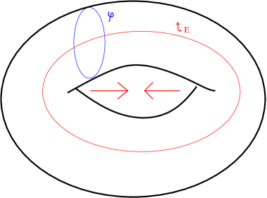
Figure 2:

Before answering this question, it is instructive to look at :

1) The analogous situation for black holes, i.e what is the relevant Euclidean manifold that correctly describes black hole entropy?

2) Computations of de Sitter entropy in Lorentzian/Euclidean approaches.

We restrict ourselves to a study of entropy computations of the BTZ black hole [16] also in $(2+1)$ dimensions but with a negative cosmological constant - as there are many similarities with our case. The entropy computations exploit the connection between gravity in three dimensions and Chern-Simons theory [17] and the relevant degrees of freedom are degrees of freedom of a Chern-Simons theory on a manifold with boundary. It is well-known that standard Euclidean continuations of black hole spacetimes describe the region from the horizon to infinity and the horizon is a degenerate surface in the Euclidean manifold. It has been shown in [18] that the Euclidean continuation of the BTZ black hole is a solid torus. The horizon is a degenerate circle at the core of the solid torus parametrised by an angular coordinate $\phi$ and situated at $r=0$ in Schwarzschild-like coordinates. The Euclidean time is now the contractible cycle of this solid torus. A partition function for this black hole in the Euclidean path integral approach has been derived in [19] using results from Chern-Simons theory. It was shown before in [13] that the leading contribution to the entropy could be obtained by considering boundary degrees of freedom of Chern-Simons theory, where the boundary is a ‘stretched horizon’. The horizon itself is a circle, and the stretched horizon is a torus tube surrounding this horizon, i.e at a small non-zero value of $r$. One then imposes invariance under residual diffeomorphisms (after imposition of boundary conditions) on the boundary states at the stretched horizon. This yields the correct semi-classical entropy on counting the states.

Now, looking at the analytic continuation of de Sitter from this perspective, we see that the de Sitter static patch is like ‘the inside’ of the black hole, i.e the horizon is now the outer, rather than the inner boundary of the physically accessible spacetime. In the BTZ case, the Euclidean topology is a solid torus. Euclidean time is a contractible cycle of the solid torus that shrinks to zero at the horizon. The horizon itself is a degenerate circle at the core of the solid torus. However, the stretched horizon at $r>0$ is not a circle but a torus. In the Euclidean de Sitter, we again have a solid torus topology - but Euclidean time is now the non-contractible cycle. We have a degenerate case at the horizon $r=1$, where the non-contractible cycle degenerates to a point - changing the topology from solid torus to the hemisphere. However, the stretched horizon is now at a value $r<1$, and its topology is again a torus as before. Considering the region from $r=0$ to the stretched horizon, the topology is that of a solid torus. Thus if the degrees of freedom corresponding to the entropy reside on the stretched horizon, the three-dimensional topology of interest is a solid torus.

Let us examine the various computations of de Sitter entropy both in the Lorentzian and Euclidean approaches. Maldacena and Strominger [6] have used the Chern-Simons formulation of three-dimensional gravity to describe the entropy. They consider Chern-Simons theory on the Lorentzian static patch manifold - which is $D_{2}\otimes R$. Then, boundary conditions are imposed on the fields at the cylindrical boundary which is the horizon. These boundary conditions are motivated by earlier work on BTZ black holes [20] and encode the fact that the boundary is an apparent horizon. Then, a WZW conformal field theory is induced on this boundary. The physical states must obey the remnant of the Wheeler-de Witt equation, i.e invariance under diffeomorphisms which preserve the boundary conditions. A simple counting of states gives the correct entropy, and the states lie on the cylindrical boundary. If an analogous computation were attempted in the Euclidean picture, it seems that the degrees of freedom on the cylindrical boundary would now be the degrees of freedom on the torus obtained by compactifying time. Also, as we saw in the Euclidean BTZ entropy computation, the imposition of the remnant of the Wheeler-de Witt equation will have to be done at the stretched horizon, as the horizon itself is a degenerate surface in the Euclidean picture. Considering the stretched horizon in the Euclidean de Sitter case implies as mentioned before, that the relevant Euclidean manifold is a solid torus.

There have been Euclidean computations using the solid torus topology. In [1], it was claimed that the relevant space was an infinitesimal tube around the timelike observer, which on Euclideanisation is a solid torus. More recently, a partition function for de Sitter space was proposed [2] using results from Chern-Simons theory on a solid torus. From this computation, it is clear that the partition function is independent of the location of the toral boundary. This computation gives the correct semi-classical entropy and also predicts a first order correction to this entropy, which agrees with corrections obtained from other unrelated approaches, like the dS/CFT correspondence.

4 Generalisation to higher dimensions

The above discussion strongly points to the relevant Euclidean manifold for computing $dS_{3}$ entropy being a solid torus. But we have argued this taking specific instances in three dimensions, which use the connection between Chern-Simons theory and gravity. A natural question to ask would be, how much of this generalises to higher dimensions? The Euclideanisation of $n$-dimensional global $dS_{n}$ is an $n$-sphere - and by previous arguments, the Euclidean continuation of the region relevant to each timelike observer is an $n$-hemisphere. Likewise, the static patch has a topology $B_{n-1}\otimes R$ - where $B_{n-1}$ is an $(n-1)$ dimensional solid ball, and $R$ denotes the time direction. The Euclidean continuation of this, for $r<1$ (horizon) is $B_{n-1}\otimes S^{1}$. Including $r=1$ makes this manifold an $n$-hemisphere. Although many aspects of the discussions in the previous sections are specific to three dimensions, it is true that in a Euclidean continuation of a static metric with horizon, the horizon becomes a degenerate surface. Thus in an entropy computation involving boundary conditions at the horizon, in the Euclidean continuation, the boundary conditions must be imposed at the stretched horizon. It is therefore likely that the importance of the stretched horizon in Euclidean computations of black hole entropy may be general, and valid in any dimension. This suggests that in any physical situation involving the region of $dS_{n}$ seen by the timelike observer, particularly for understanding entropy, the correct topology in the Euclidean picture is $B_{n-1}\otimes S^{1}$. It would be interesting to explore the consequences of such an idea in cosmological situations.

References

- [1] M. Banados, T. Brotz and M. Ortiz, Phys. Rev. D59, 046002 (1999).
- [2] T. R. Govindarajan, R. K. Kaul and V. Suneeta, Class. Quant. Grav. 19, 4195 (2002).
- [3] A. Strominger, JHEP 0110, 034 (2001).
- [4] S. Nojiri and S.D. Odintsov, Phys. Lett. B519, 145 (2001).
- [5] D. Klemm, Nucl. Phys. B625, 295 (2002).
- [6] J. Maldacena and A. Strominger, JHEP 9802, 014 (1998).
- [7] F. Lin and Y. Wu, Phys. Lett. B453, 222 (1999).
- [8] Mu-In Park, Phys. Lett. B440, 275 (1998).
- [9] V. Balasubramanian, J. de Boer and D. Minic, Mass, entropy and holography in asymptotically de Sitter spaces, hep-th/0110108.
- [10] Y. S. Myung, Mod. Phys. Lett. A16, 2353 (2001).
- [11] D. Kabat and G. Lifschytz, de Sitter entropy from conformal field theory, hep-th/0203083.
- [12] R. Bousso, JHEP 0011, 038 (2000).
- [13] S. Carlip, Phys. Rev. D55, 878 (1997).
- [14] S. Deser, R. Jackiw and G.’t Hooft, Annals Phys. 152, 220 (1984).
- [15] S. Deser and R. Jackiw, Annals Phys. 153, 405 (1984).
- [16] M. Banados, C. Teitelboim and J. Zanelli, Phys. Rev. Lett. 69, 1849 (1992).
- [17] A. Achucarro and P. Townsend, Phys. Lett. B180, 89 (1986).
- [18] S. Carlip and C. Teitelboim, Phys. Rev. D51, 622 (1995).
- [19] T. R. Govindarajan, R. K. Kaul and V. Suneeta, Class. Quant. Grav. 18, 2877 (2001).
- [20] S. Carlip, Phys. Rev. D51, 632 (1995).