hep-th/0209139

Instanton Number of
Noncommutative U(n) gauge theory

Akifumi Sako
Graduate School of Science, Hiroshima University,
1-3-1 Kagamiyama, Higashi-Hiroshima 739-8526, Japan

ABSTRACT

We show that the integral of the first Pontrjagin class is given by an integer and it is identified with instanton number of the $U(n)$ gauge theory on noncommutative ${\bf R^{4}}$. Here the dimension of the vector space $V$ that appear in the ADHM construction is called Instanton number. The calculation is done in operator formalism and the first Pontrjagin class is defined by converge series. The origin of the instanton number is investigated closely, too.

1 Introduction

Recently, there has been much interest in noncommutative field theory motivated by the string theory and we can see it in [5, 8, 32, 9] and so on. These discoveries show us the nonperturbative analysis of noncommutative gauge theory is very important for the string theory. Especially, instantons play the most essential role in nonperturbative analysis. In commutative theory, there is a well-known method to construct instanton solution, which is given by Atiyah, Drinfeld, Hitchin and Manin (ADHM) [1, 7, 29]. There is the one-to-one correspondence between the instanton solutions and the ADHM data. On the other hand, in noncommutative spaces case, a pioneering work for instantons was done by Nekrasov and Schwarz [26]. They discovered deformed ADHM method to construct instanton of noncommutative gauge theory. This deformation corresponds to the resolution of instanton moduli space [25]. After that, many progress are reported about noncommutative instanton. For example, multi instanton solution of noncommutative U(1) gauge theory is given in [16], where the solution was discovered by the deformation of the commutative case solution [2]. Recently, Atiyah-Singer Index theorem for the noncommutative theory is discussed in [20], that is related deeply with the instanton number. Other important progress are in [10, 14, 27, 28, 24, 3, 18, 19, 6, 23, 22, 21].

Instanton is classified by topological charge that is called instanton number. In commutative case, instanton number is given by the integral of the 1st. Pontrjagin class and it is equivalent to ${\rm dim}~{}V$ in the ADHM construction (see the next section). However in noncommutative gauge theory, many problems had been left for the defining the integer-valued Pontrjagin class, and we had never found the proof to show that the instanton number of $U(n)$ gauge theory is identified with the integral of the Pontrjagin class. Here we define “instanton number” by the ${\rm dim}~{}V$, where $V$ is a complex vector space i.e.$V={\bf C}^{k}$ and it appears in ADHM construction (see section 2). (Thinking over the correspondence with the commutative case, we had better use the name “instanton number”for the integral of the first Pontrjagin class. But the noncommutative instanton is discovered with ADHM construction and the “instanton number” is used as the dimension of vector space $V$ in ADHM construction after [26]. So, we are in accordance with this convention.) For the noncommutative $U(1)$ theory and some special $U(n)$ cases that are essentially same as $U(1)$ case, Furuuchi explained the origin of the instanton number and identity between the instanton number and the Pontrjagin class [10, 11, 13]. Its strict proof was given in [17]. These cases are easy to calculate instanton charge because we can put $J=0$ , where $J$ is $Hom(V,~{}{\bf C^{n}})$ in ADHM data. But we cannot adapt the condition $J=0$ to general $U(n)$ case. This had been the difficulty for proof for $U(n)$.

The aim of this article is to give the proof of identification between the integral of the first Pontrjagin class and ${\rm dim}~{}V$ for noncommutative $U(n)$ theory. As same as [17], the integer-valued Pontrjagin class is defined by the converge series. The calculation is carried out by different way from [17] because we can not use $J=0$ condition. As a result of the different way of the calculation, we can easily see the direct relation between ${\rm dim}~{}V$ and integral of the first Pontrjagin class and we can understand noncommutativity play a very important role there. To clarify the distinction, we call the integral of the first Pontrjagin class “instanton charge” and call $\dim$ of vector space $V$ “instanton number”.

The organization of this paper is as follows. In section 2, we review the noncommutative instanton and prepare tools of instanton charge calculus. In section 3, some lemmas are given to study the origin of the instanton number, and some of them are necessary to calculate the instanton charge. In section 4, we prove that the integral of the first Pontrjagin class is equal to ${\rm dim}~{}V$. In section 5, we summarize this article.

2 Noncommutative $U(n)$ Instantons

We introduce the noncommutative field theory used in this article and review the noncommutative instantons, in this section.

2.1 Noncommutative $\bf{R}^{4}$ and the Fock space representation

Let us consider Euclidean noncommutative $\bf{R}^{4}$. Its coordinate operators $x^{\mu}\;(\mu=1,2,3,4)$ on the noncommutative manifold satisfy the following commutation relations

$$[x^{\mu},x^{\nu}]=i\theta^{\mu\nu},$$ (1)

where $\theta^{\mu\nu}$ is an antisymmetric real constant matrix, whose elements are called noncommutative parameters. We can always bring $\theta^{\mu\nu}$ to the skew-diagonal form

$$\theta^{\mu\nu}=\begin{pmatrix}0&\theta^{12}&0&0\\ -\theta^{12}&0&0&0\\ 0&0&0&\theta^{34}\\ 0&0&-\theta^{34}&0\end{pmatrix}$$ (2)

by space rotation. We restrict the noncommutativity of the space to the self-dual case of $\theta^{12}=\theta^{34}=-\zeta\$. In this article, we perform the calculation with this condition, but $|\theta^{12}|=|\theta^{34}|$ is not essential. This is only for convenience. On the other hand, relative sign of the noncommutative parameter ( $\theta^{12}\theta^{34}>0$ ) is significant and it is discussed in the section 5. Here we introduce complex coordinates

$$z_{1}=\frac{1}{\sqrt{2}}(x^{1}+ix^{2}),\;\;z_{2}=\frac{1}{\sqrt{2}}(x^{3}+ix^{4}),$$ (3)

then the commutation relations (1) become

$$[z_{1},\bar{z}_{1}]=[z_{2},\bar{z}_{2}]=-\zeta,\;\;\mbox{others are zero}.$$ (4)

For using the usual operator representation, we define creation and annihilation operators by

$$c^{{\dagger}}_{\alpha}=\frac{z_{\alpha}}{\sqrt{\zeta}},\;\;c_{\alpha}=\frac{\bar{z}_{\alpha}}{\sqrt{\zeta}},\;\;[c_{\alpha},c^{{\dagger}}_{\alpha}]=1\;\;\;\;(\alpha=1,2).$$ (5)

The Fock space $\cal H$ on which the creation and annihilation operators (5) act is spanned by the Fock state

$$\left|n_{1},n_{2}\right>=\frac{(c^{{\dagger}}_{1})^{n_{1}}(c^{{\dagger}}_{2})^{n_{2}}}{\sqrt{n_{1}!n_{2}!}}\left|0,0\right>,$$ (6)

with

$$c_{1}\left|n_{1},n_{2}\right>=\sqrt{n_{1}}\left|n_{1}-1,n_{2}\right>,\;\; c^{{\dagger}}_{1}\left|n_{1},n_{2}\right>=\sqrt{n_{1}+1}\left|n_{1}+1,n_{2}\right>,$$

$$c_{2}\left|n_{1},n_{2}\right>=\sqrt{n_{2}}\left|n_{1},n_{2}-1\right>,\;\; c^{{\dagger}}_{2}\left|n_{1},n_{2}\right>=\sqrt{n_{2}+1}\left|n_{1},n_{2}+1\right>,$$ (7)

where $n_{1}$ and $n_{2}$ are the occupation number. The number operators are also defined by

$$\hat{n}_{\alpha}=c^{{\dagger}}_{\alpha}c_{\alpha},\;\;\hat{N}=\hat{n}_{1}+\hat{n}_{2},$$ (8)

which act on the Fock states as

$$\hat{n}_{\alpha}\left|n_{1},n_{2}\right>=n_{\alpha}\left|n_{1},n_{2}\right>,\;\;\hat{N}\left|n_{1},n_{2}\right>=(n_{1}+n_{2})\left|n_{1},n_{2}\right>.$$ (9)

In the operator representation, derivatives of a function $f(z_{1},\bar{z}_{1},z_{2},\bar{z}_{2})$ are defined by

$$\partial_{\alpha}f(z)=[\hat{\partial}_{\alpha},f(z)],\hskip 14.22636pt\partial_{\bar{\alpha}}f(z)=[\hat{\partial}_{\bar{\alpha}},f(z)],$$ (10)

where $\hat{\partial}_{\alpha}=\bar{z}_{\alpha}/\zeta$, $\hat{\partial}_{\bar{\alpha}}=-z_{\alpha}/\zeta$ which satisfy

$$[\hat{\partial}_{\alpha},\hat{\partial}_{\bar{\alpha}}]=-\frac{1}{\zeta}.$$ (11)

The integral on noncommutative $\bf{R}^{4}$ is defined by the standard trace in the operator representation,

$$\int d^{4}x=\int d^{4}z=(2\pi\zeta)^{2}\mbox{Tr}_{\cal H}.$$ (12)

Note that $\mbox{Tr}_{\cal H}$ represents the trace over the Fock space whereas the trace over the gauge group is denoted by $\mbox{tr}_{U(n)}$.

2.2 Noncommutative gauge theory and instantons

Let us consider the $U(n)$ Yang-Mills theory on noncommutative $\bf R^{4}$. Let $M$ be a projective module over the algebra that is generated by the $x_{\mu}$ satisfying (1).

In the noncommutative space, the Yang-Mills connection is defined by

$$\hat{\nabla}_{\mu}\psi=-\psi\hat{\partial}_{\mu}+\hat{D}_{\mu}\psi,$$ (13)

where $\psi$ is a matter field in fundamental representation type and $D_{\mu}\in End(M)$ are anti-hermitian gauge fields [27][28][14]. The relation between $D_{\mu}$ and usual gauge connection $A_{\mu}$ is $D_{\mu}=-i\theta_{\mu\nu}x^{\nu}+A_{\mu}$, where $\theta_{\mu\nu}$ is an inverse matrix of $\theta^{\mu\nu}$ in (1). Then the Yang-Mills curvature of the connection $\nabla_{\mu}$ is

$$F_{\mu\nu}=[\hat{\nabla}_{\mu},\hat{\nabla}_{\nu}]=-i\theta_{\mu\nu}+[{\hat{D}}_{\mu},{\hat{D}}_{\nu}].$$ (14)

In our notation of the complex coordinates (3) and (4), the curvature (14) is

$$F_{\alpha\bar{\alpha}}=\frac{1}{\zeta}+[{\hat{D}}_{\alpha},{\hat{D}}_{\bar{\alpha}}],\hskip 14.22636ptF_{\alpha\bar{\beta}}=[{\hat{D}}_{\alpha},{\hat{D}}_{\bar{\beta}}]\hskip 28.45274pt(\alpha\not=\beta).$$ (15)

The Yang-Mills action is given by

$$S=-\frac{1}{g^{2}}{\rm Tr}_{\cal H}\mbox{tr}_{U(n)}F\wedge*F,$$ (16)

where we denote ${\rm tr}_{U(n)}$ as a trace for the gauge group U(n), $g$ is the Yang-Mills coupling and $*$ is Hodge-star.

Then the equation of motion is

$$[\nabla_{\mu},F_{\mu\nu}]=0.$$ (17)

(Anti-)instanton solutions are special solutions of (17) which satisfy the (anti-)self-duality ((A)SD) condition

$$F=\pm*F.$$ (18)

These conditions are rewritten in the complex coordinates as

$$F_{1\bar{1}}= + F_{2\bar{2}},\;\;F_{1\bar{2}}=F_{\bar{1}2}=0\;\;\;\;\mbox{(self-dual)},$$ (19)

$$F_{1\bar{1}}= - F_{2\bar{2}},\;\;F_{12}=F_{\bar{1}\bar{2}}=0\;\;\;\;\mbox{(anti-self-dual)}.$$ (20)

In the commutative spaces, solutions of Eq.(18) are classified by the topological charge (integral of the first Pontrjagin class)

$$Q=-\frac{1}{8\pi^{2}}\int\mbox{tr}_{U(n)}F\wedge F,$$ (21)

which is always integer and called instanton number $k$. However, in the noncommutative spaces above statement is unclear. We discuss this issue in this article by using the operator representation of (21)

$$Q=\begin{cases}\zeta^{2}\mbox{Tr}_{\cal H}\,\mbox{tr}_{U(n)}(F_{1\bar{1}}F_{2\bar{2}}-F_{12}F_{\bar{1}\bar{2}})\;\;\;\;&\mbox{(self-dual)}\\ \zeta^{2}\mbox{Tr}_{\cal H}\,\mbox{tr}_{U(n)}(F_{1\bar{1}}F_{2\bar{2}}-F_{1\bar{2}}F_{2\bar{1}})\;\;\;\;&\mbox{(anti-self-dual)}.\end{cases}$$ (22)

Note that this definition of instanton charge is naive one. For determination of the instanton charge, trace operation have to be defined by the summation over finite domain of the Fock space and the instanton charge have to be defined by a converge series. These conditions are discussed in the following sections.

In this article, all studies and discussions are done for ASD case, but they are adapted for SD case.

2.3 Noncommutative $U(n)$ instantons

In the ordinary commutative spaces, there is a well-known way to find ASD configurations of the gauge fields. It is ADHM construction which is proposed by Atiyah, Drinfeld, Hitchin and Manin [1]. Nekrasov and Schwarz first extended this method to noncommutative cases [26]. Here we review briefly the ADHM construction of $U(n)$ instantons[27][28].

The first step of ADHM construction on noncommutative $R^{4}$ is looking for $B_{1},B_{2}\in End({\bf C}^{k})$, $I\in Hom({\bf C}^{n},{\bf C}^{k})$ and $J\in Hom({\bf C}^{k},{\bf C}^{n})$ which satisfy the deformed ADHM equations

$$[B_{1},B_{1}^{{\dagger}}]+[B_{2},B_{2}^{{\dagger}}]+II^{{\dagger}}-J^{{\dagger}}J=2\zeta,$$ (23)

$$[B_{1},B_{2}]+IJ=0.$$ (24)

We call this $k$ “instanton number”. In the previous section and abstract, $V$ denotes the vector space ${\bf C}^{k}$. Note that the right hand side of Eq.(23) is caused by the noncommutativity of space. The set of $B_{1},B_{2},I$ and $J$ is called ADHM data. Using this ADHM data, we define operator ${\cal D}:{\bf C}^{k}\oplus{\bf C}^{k}\oplus{\bf C}^{n}\rightarrow{\bf C}^{k}\oplus{\bf C}^{k}$ by

$${\cal D} = \left(\begin{array}[]{c}\tau\\ \sigma^{\dagger}\end{array}\right)$$ (27)

$$\tau = (B_{2}-z_{2},B_{1}-z_{1},I)=(B_{2}-\sqrt{\zeta}c_{2}^{\dagger},B_{1}-\sqrt{\zeta}c_{1}^{\dagger},I)$$

$$\sigma^{\dagger} = (-B^{\dagger}_{1}+\bar{z}_{1},B^{\dagger}_{2}-\bar{z}_{2},J^{\dagger})=(-B^{\dagger}_{1}+\sqrt{\zeta}c_{1},B^{\dagger}_{2}-\sqrt{\zeta}c_{2},J^{\dagger}).$$ (28)

ADHM eqs. (23) and (24) are replaced by

$$\tau\tau^{\dagger}=\sigma^{\dagger}\sigma\equiv\square,\ \ \tau\sigma=0.$$ (29)

The following fact about this $\square$ is known.

Lemma 2.0.1 (Absence of zero-mode of $\square$)

There is no zero-mode of $\square$. That is, for ${}^{\forall}\lvert v\rangle\in{\cal H}\otimes{\bf C}^{k}$,

$$\square\lvert v\rangle=0\ \to\ \lvert v\rangle=0.$$ (30)

Proof of this lemma is given by Furuuchi in the Appendix A of [10] or by Nekrasov in the section 4.2 of [27].

Let $\Psi$ be the solutions of the equations:

$${\cal D}\Psi^{a}=0\ \ (a=1,\cdots,n) ,\ \ \ \Psi^{a}:{\bf C}^{n}\rightarrow{\bf C}^{k}\oplus{\bf C}^{k}\oplus{\bf C}^{n},$$ (31)

$$\Psi^{\dagger a}\Psi^{b} = \delta^{ab}\ .$$ (32)

Then we can construct the $U(n)$ $k$ instanton(ASD) connection $D_{\mu}$ in (14) as

$$D_{\mu}=i\Psi^{\dagger}\theta_{\mu\nu}x^{\nu}\Psi.$$ (33)

With the complex coordinate $z_{\alpha}$, they are rewritten as

$$D_{\alpha}=\frac{1}{\zeta}\Psi^{\dagger}\bar{z_{\alpha}}\Psi\ \ \ D_{\bar{\alpha}}=-\frac{1}{\zeta}\Psi^{\dagger}{z_{\alpha}}\Psi.$$ (34)

Let us enumerate important identities here. They are obeyed from (32),(23), (24) and (29). At first,

$$\Psi\Psi^{\dagger}=1-{\cal D}^{\dagger}\frac{1}{{\cal DD}^{\dagger}}{\cal D}.$$ (35)

This is the most useful identity in this paper. $\Psi\Psi^{\dagger}$ and ${\cal D}^{\dagger}\frac{1}{{\cal DD}^{\dagger}}{\cal D}$ are projectors. $\Psi\Psi^{\dagger}$ projects out the eigenvectors of ${\cal D}^{\dagger}\frac{1}{{\cal DD}^{\dagger}}{\cal D}$. In other words, there are $\Psi\Psi^{\dagger}$ zero modes, which are given by ${\cal D}^{\dagger}\frac{1}{{\cal DD}^{\dagger}}{\cal D}$ eigen state. In section 3, we investigate them closely. This operators are expressed with $\tau$ and $\sigma$ as

$${\cal DD}^{\dagger}=\left(\begin{array}[]{cc}\square&0\\ 0&\square\end{array}\right),\ \ \ {\cal D}^{\dagger}\frac{1}{{\cal DD}^{\dagger}}{\cal D}=\tau^{\dagger}\frac{1}{\square}\tau+\sigma\frac{1}{\square}\sigma^{\dagger}.$$ (38)

These relations are going to be used in the calculation for the instanton charge several times.

3 Zero modes of $\Psi\Psi^{\dagger}$ and its nature

In this section, we prepare to calculate the instanton charge (integral of the Pontrjagin class) and analyze the source of the instanton charge. It is expected that the instanton charge is integer and equal to instanton number as same as commutative case. The aim of this article is to give the proof of this statement. It is given in the section 4, but the method used in the proof is differ from the one used for $U(1)$ case. Therefore, the relation between $U(1)$ and $U(n)$ about the origin of the instanton charge is not understood by the calculus in the section 4. To supplement explanation for it, we study the origin of the instanton charge by the similar way of the $U(1)$ case [17].

3.1 Zero-mode of $\Psi\Psi^{\dagger}$

It is convenience to give some lemmas that describe the detail of the zero-mode of $\Psi\Psi^{\dagger}$.

Lemma 3.0.1 (Zero-mode of $\Psi\Psi^{\dagger}$)

Suppose that $\Psi$ and $\Psi^{\dagger}$ are given in the previous section. The vector $\lvert v\rangle\in({\bf C}^{k}\oplus{\bf C}^{k}\oplus{\bf C}^{n})\otimes{\cal H}$ satisfying

$$\Psi\Psi^{\dagger}\lvert v\rangle=\langle v\rvert\Psi\Psi^{\dagger}=0,\ \ \lvert v\rangle\neq 0$$ (39)

is said to be a zero mode of $\Psi\Psi^{\dagger}$. Then the zero-modes are given by following three types:

$$\lvert v_{1}\rangle=\left(\begin{array}[]{c}(-B_{1}+\sqrt{\zeta}c_{1}^{\dagger})\lvert u\rangle\\ (B_{2}-\sqrt{\zeta}c_{2}^{\dagger})\lvert u\rangle\\ J\lvert u\rangle\end{array}\right),\ \ \lvert v_{2}\rangle=\left(\begin{array}[]{c}(B^{\dagger}_{2}-\sqrt{\zeta}c_{2})\lvert u^{\prime}\rangle\\ (B^{\dagger}_{1}-\sqrt{\zeta}c_{1})\lvert u^{\prime}\rangle\\ I^{\dagger}\lvert u^{\prime}\rangle\end{array}\right)$$ (46)

$$\lvert v_{0}\rangle=\left(\begin{array}[]{c}(\exp\frac{1}{\sqrt{\zeta}}\sum_{\alpha}B^{\dagger}_{\alpha}c^{\dagger}_{\alpha})\lvert 0,0\rangle v_{0}^{i}\\ (\exp\frac{1}{\sqrt{\zeta}}\sum_{\alpha}B^{\dagger}_{\alpha}c^{\dagger}_{\alpha})\lvert 0,0\rangle v_{0}^{i}\\ 0\end{array}\right).$$ (50)

Here $\lvert u\rangle$ ($\lvert u^{\prime}\rangle$) is some element of ${\bf C}^{k}\otimes{\cal H}$ (i.e. $\lvert u\rangle$ is expressed with the coefficients $u^{nm}_{i}\in{\bf C}$ as $\lvert u\rangle=\sum_{i}\sum_{n,m}u^{nm}_{i}\lvert n,m\rangle e_{i}$ , where $e_{i}$ is a base of $k$-dim vector space ). $v_{0}^{i}$ is a element of $k$-dim vector.

Proof. From eq.(35), $\Psi\Psi^{\dagger}$ have a zero-mode as an eigenvector of the operator ${\cal D}^{\dagger}\frac{1}{{\cal DD}^{\dagger}}{\cal D}$. (In the following we call eigenvector of the operator ${\cal D}^{\dagger}\frac{1}{{\cal DD}^{\dagger}}{\cal D}$ “${\cal D}$ eigenvectors”. “$\tau$ eigenvector” is used similarly.) By the Eqs.(29), ${\cal D}$ eigen vectors are classified as eigen vectors of $\tau$ or $\sigma^{\dagger}$. The equation $\tau\sigma=0$ show that the $\lvert v_{1}\rangle$ ($\lvert v_{2}\rangle$) is in $\ker\tau$ ($\ker\sigma^{\dagger}$).

$$\tau\lvert v_{1}\rangle=\tau\sigma\lvert u\rangle=0,\ \sigma^{\dagger}\lvert v_{2}\rangle=\sigma^{\dagger}\tau^{\dagger}\lvert u^{\prime}\rangle=0.$$ (51)

If $\lvert u\rangle$ and $\lvert u^{\prime}\rangle$ are not zero vectors, as a result of the lemma2.0.1,

$$\sigma^{\dagger}\lvert v_{1}\rangle=\sigma^{\dagger}\sigma\lvert u\rangle=\square\lvert u\rangle\neq 0 \ \tau\lvert v_{2}\rangle=\tau\tau^{\dagger}\lvert u^{\prime}\rangle=\square\lvert u^{\prime}\rangle\neq 0.$$ ,

$${\cal D}^{\dagger}\frac{1}{{\cal DD}^{\dagger}}{\cal D}\lvert v_{1}\rangle=\sigma\lvert u\rangle=\lvert v_{1}\rangle \ \ {\cal D}^{\dagger}\frac{1}{{\cal DD}^{\dagger}}{\cal D}\lvert v_{2}\rangle=\lvert v_{2}\rangle.$$ , (52)

If we chose $k$ independent vectors $\sum_{nm}u^{nm}_{i}\lvert n,m\rangle$ ($i=(1,\cdots,k)$) and orthonormalize them, we get ${\cal D}$ $k$-dim eigen vector space that is zero-mode space of $\Psi\Psi^{\dagger}$. $\sum_{nm}{u^{\prime}}^{nm}_{i}\lvert n,m\rangle$ is similar to $\sum_{nm}u^{nm}_{i}\lvert n,m\rangle$ and we can construct other $k$-dim zero-mode space.
The remnant of this proof is for $\lvert v_{0}\rangle$. From commutation relations,

$$\sigma^{\dagger}\lvert v_{0}\rangle=0,$$ (53)

and it shows that $\lvert v_{0}\rangle$ is belong to the eigen vectors of $\tau$. From the following relation, it is shown that $\lvert v_{0}\rangle$ is independent from the $\lvert v_{2}\rangle$,

$$\langle v_{0}|v_{2}\rangle=0.$$ (54)

After we orthonormalize them, it is concluded that they are eigen vectors of ${\cal D}$ and zero-modes of $\Psi\Psi^{\dagger}$.

$\square$

We are going to know the zero-mode $\lvert v_{0}\rangle$ corresponds to the source of the instanton charge and this zero-mode plays a essential role when we introduce cut-off (boundary) for the Fock space. This lemma is not directly used in the instanton charge computation in section 4. But this is important when we understand the origin of the instanton charge by the parallel way of $U(1)$ instanton case.

3.2 Boundary

In the [16, 17], we introduced the Fock space cut-off $N$. The cut off make the instanton charge be a converge series and be a meaningful in these papers. So we introduce cut-off, again. But some complex rules of cut-off boundary or trace operation occur as a result of the zero-mode $\lvert v_{0}\rangle$. At first, let us study the rules.

As the simplest example, we review the $U(1)$ case in [16, 17]. In these paper, we set the cut-off in the $n_{1}$ and $n_{2}$ directions on $N$ ($N\gg k$) (Fig.2), here the “cut-off” means the trace operation cut-off, that is,

$${\rm Tr}_{\cal H}\left|{}_{\scriptscriptstyle[0,~{}N]}O\right.=\sum_{n_{1}=0}^{N}\sum_{n_{2}=0}^{N}\left<n_{1},n_{2}\right|O\left|n_{1},n_{2}\right>\;,$$ (55)

where $O$ is an arbitrary operator. Note that this cut off is only for the upper bound of summation of the initial state and the final state. To the contrary, upper bound of intermediate summation is frequently over $N$. In the $U(1)$ case (and $J=0$ case of $U(n)$), we can construct the instanton connection with the shift operator apparently. The shift operator cause the shift of the boundary for the summation over intermediate states (see Fig.2).

\psfragscanon\psfrag{n1}[1.5]{$n_{1}$}\psfrag{n2}[1.5]{$n_{2}$}\psfrag{0}[1.5]{$0$}\psfrag{p1}[1.5]{$k-1$}\psfrag{p2}[1.5]{1}\psfrag{c1}[1.5]{$N$}\psfrag{c2}[1.5]{$N$}\psfrag{P}[1.5]{$P$}\psfrag{R}[2.0]{$\underline{\it D}$}\includegraphics{Figures/region0.eps}

Figure 1: Region of $\mbox{Tr}_{\cal H}$ operation; This represents the region of summation of $\mbox{Tr}_{\cal H}$ operation. We set the cut-off of the Fock space in the $n_{1}$ and $n_{2}$ direction at $N$ in [17].

\psfragscanon\psfrag{n1}[1.5]{$n_{1}$}\psfrag{n2}[1.5]{$n_{2}$}\psfrag{0}[1.5]{$0$}\psfrag{p1}[1.5]{$k-1$}\psfrag{p2}[1.5]{$0$}\psfrag{c1}[1.5]{$N$}\psfrag{c2}[1.5]{$N$}\psfrag{P}[1.5]{$v_{0}$}\psfrag{R}[2.0]{$\bar{D}$}\psfrag{s1}[1.5]{$N+k$}\includegraphics{Figures/regionS.eps}

Figure 2: Region of the intermediate states; This represents the region of intermediate summation of the Fock space. Intermediate states appear inside of operators $\Psi^{\dagger}$ and $\Psi$ in the U(n) ($S$ and $S^{{\dagger}}$ in the U(1) ) case.

In [16, 17], $N\times N$ square was chosen for the boundary of initial and final state. The instanton charge do not depend on the shape of the Fock space region. For example, $N_{1}\times N_{2}$ rectangle or triangle that is defined by $n_{1}+n_{2}=N$ are simple boundary for calculation. In either case, we can get the same result of instanton charge.

To clarify the independence of the result from the shape of the boundary, we do not make concrete shape of boundary, here. Only the characteristic size of domain is introduced by $N$. The region of the initial and final state of Fock space with the boundary is a set of states:

$$\lvert n_{1},n_{2}\rangle;n_{1}=0,\cdots,N_{1}(n_{2})\ \ n_{2}=0,\cdots,N_{2}(n_{1}),$$ (56)

where $N_{1}(n_{2})$ ($N_{2}(n_{1})$) is a function of $n_{2}$ ($n_{1}$) and we suppose that length of the boundary is order $N\gg k$ i.e. $N_{1}(n_{2})\approx N_{2}(n_{1})\approx N\gg k$ ( see Fig.3).

\psfragscanon\psfrag{n1}[1.5]{$n_{1}$}\psfrag{n2}[1.5]{$n_{2}$}\psfrag{c1}[1.5]{$O(N)$}\psfrag{c2}[1.5]{$O(N)$}\psfrag{0}[1.5]{$0$}\psfrag{m}[1.5]{$m$}\psfrag{l}[1.5]{$l$}\psfrag{nm}[1.5]{$N_{1}(m)$}\psfrag{nl}[1.5]{$N_{2}(l)$}\includegraphics{Figures/explain-N1m-N2l.eps}

Figure 3: $N_{1}(m)$, $N_{2}(l)$: The set of the Fock states is surrounded by the boundary whose length is order $N$. $N_{1}(N_{2})$ depends on $n_{1}(n_{2})$.

Using this cut-off (boundary), we define the instanton charge (integral of the first Pontrjagin class) by

$$Q = \lim_{N\rightarrow\infty}Q_{N},$$ (57)

$$Q_{N} = \zeta^{2}\sum_{n_{1}=0}\sum_{n_{2}=0}^{N_{2}(n_{1})}\left<n_{1},n_{2}\right|(F_{1\bar{1}}F_{2\bar{2}}-F_{1\bar{2}}F_{2\bar{1}})\left|n_{1},n_{2}\right>.$$ (58)

One problem is left to determine (58), that is to define the region of the Fock space of intermediate state. As [17] case, the region for summation of intermediate state is shifted. This phenomena is caused by the existence of the $\Psi\Psi^{\dagger}$ zero-mode. Therefore we have to introduce the different region for intermediate state. (The state, which is sandwiched by $\Psi^{\dagger}$ from left and $\Psi$ from right, is calld “intermediate state”.) For introducing it, the following remark is important.

Remark 3.0.1 (Dimension of the zero-modes)

Consider the region of the Fock state as $\{(n_{1},n_{2})|0<n_{1}<\underline{{\it N}}_{1}(n_{2}),0<n_{2}<\underline{{\it N}}_{2}(n_{1})\}$. (Under bar of $\underline{{\it N}}_{i}$ discriminate between boundary of initial states and one of intermediate state.) If the boundary shape is convex, then there is $\underline{{\it N}}$ dimension Fock state vector ,where

$$\underline{{\it N}}\equiv\sum_{n_{2}=0}(\underline{{\it N}}_{1}(n_{2})+1)=\sum_{n_{1}=0}(\underline{{\it N}}_{2}(n_{1})+1).$$ (59)

Here $\sum_{n_{2}}(\underline{{\it N}}_{1}(n_{2})+1)$ is the area of the region of the Fock state. ($n_{1}=0$ line cause “$+1$” in $(\underline{{\it N}}_{1}(n_{2})+1)$.) Taking account of this fact, we can introduce dimension for subset of Hilbert space (finite domain of the Fock space) by counting each Fock state as an independent vector. Then the dimension of the zero-modes $\left\{\lvert v_{1}\rangle\right\}$, $\left\{\lvert v_{2}\rangle\right\}$ and $\left\{\lvert v_{0}\rangle\right\}$ are $k\times\underline{{\it N}}$, $k\times\underline{{\it N}}$ and $k$.

Note that above boundary is only for one component of ($2k+n$)-dim vector (remember that $\Psi^{a}\in{\bf C}^{2k+n}\otimes{\cal H}$). In general, each component of the vector do not have universal boundary. So if the boundary is not universal, some index $i$ ($i\in\{1,\cdots,2k+n\}$) have to be introduced to assign to each boundary i.e. $\underline{{\it N}}\rightarrow\underline{{\it N}}^{i}$.
From this remark, to make $\Psi$ be an isomorphism for finite domain Fock space, the dimension of initial state should be the same dimension of intermediate state. (Note that $\Psi$ is a partial isometry, i.e. $\Psi\Psi^{\dagger}\neq 1$ for infinite dimensional Fock space, but it is possible to be regarded as an isomorphism when we consider finite domain.) For some fixed $l$ and $p$, $\Psi^{a}_{l,p,n_{1},n_{2}}\lvert n_{1},n_{2}\rangle$ is a expanded by $n\times\underline{{\it N}}$ bases. On the other hand, when left module Fock space is defined by the same domain as the right module, for some fixed $n$ and $m$, $\langle l,p\rvert\Psi^{a}_{l,p,n,m}$ is expanded by $n\times\underline{{\it N}}-k$ bases because there are $k$ zero-modes $\langle v_{0}\rvert$ that are removed from only intermediate state. Therefore we have to set the cut-off of the intermediate state as

$$\sum_{i=1}^{2k+n}\sum_{n_{2}=0}(\bar{N}^{i}_{1}(n_{2})+1)=\sum_{i=1}^{2k+n}\sum_{n_{1}=0}(\bar{N}^{i}_{2}(n_{1})+1)=(2k+n)\times\underline{{\it N}}+k,$$ (60)

where $\bar{N}^{i}_{\alpha}$ is boundary of intermediate state for $i$-th component of $(2k+n)$-dim vector. This boundary is naive extension of the $U(1)$ case (Fig.2).

Generally, it is difficult to give a concrete expression of intermediate boundary from initial state boundary. But intermediate boundary is often more necessary than initial boundary for instanton charge calculation in the next section. Therefore we define the trace operation of finite region not by initial state domain but intermediate domain, in the next section. It is tricky but very convenience definition.

It is worth to mention the essence of the above finite domain of the trace operation. It is to make $\Psi$ be an isometry for finite domain. So the domain of the intermediate state is changed by the situation. For example, consider two state $\Psi^{\dagger}\cdots\langle inter|\Psi|initial\rangle$ and $\Psi^{\dagger}\cdots\langle inter^{\prime}|c_{1}^{\dagger}\Psi|initial\rangle$. Then the domain (set) of the intermediate state $\langle inter^{\prime}|$ is given by domain of $\langle inter|$ shifted by $c_{1}^{\dagger}$. Therefore region of “intermediate state” is determined case by case.

To support the definition of the boundary and above discussions, following Remark is important.

Remark 3.0.2 (Asymptotic behavior of the $\lvert v_{0}\rangle$)

If $N_{1}+N_{2}\equiv N$ is enough large, using some positive constant $c$ and $\epsilon<1$,

$$\lvert\langle N_{1},N_{2}|\otimes 1\ |v_{0}\rangle\rvert<{c}{\epsilon^{N}}.$$ (61)

Proof. Some constant $\beta$ exists, which satisfies

$$\lvert\langle N_{1},N_{2}|\otimes 1\ |v_{0}\rangle\rvert = \left|\left(\begin{array}[]{c}\langle N_{1},N_{2}|(\exp\sum_{\alpha}B^{\dagger}_{\alpha}c^{\dagger}_{\alpha})|0,0\rangle v_{0}^{i}\\ \langle N_{1},N_{2}|(\exp\sum_{\alpha}B^{\dagger}_{\alpha}c^{\dagger}_{\alpha})|0,0\rangle v_{0}^{i}\\ 0\end{array}\right)\right|$$ (65)

$$< \left|\left(\begin{array}[]{c}\frac{\beta^{N_{1}+N_{2}}}{\sqrt{N_{1}!N_{2}!}}\\ \frac{\beta^{N_{1}+N_{2}}}{\sqrt{N_{1}!N_{2}!}}\\ 0\end{array}\right)\right|.$$ (69)

When $N_{1}+N_{2}\equiv N$ is large enough and we assume $N_{1}>N_{2}$. ($N_{2}>N_{1}$ case is proved as same as following way.) Then

$${}^{\exists}N^{\prime}\ |\ \beta<{N^{\prime}}^{\frac{1}{4}}<N^{\prime}<\frac{N}{2}.$$ (70)

Using this $N^{\prime}$,

$$\frac{\beta^{N_{1}+N_{2}}}{\sqrt{N_{1}!N_{2}!}} < \frac{\beta^{N}}{\sqrt{N_{1}!}}<\frac{\sqrt{N^{\prime}}^{\frac{N}{2}}}{\sqrt{N_{1}!}}<\frac{\sqrt{N^{\prime}}^{N_{1}}}{\sqrt{N_{1}!}}$$ (71)

$$= \frac{\sqrt{N^{\prime}}^{N^{\prime}}}{\sqrt{N^{\prime}!}}\sqrt{\frac{(N^{\prime})^{N_{1}-N^{\prime}}}{(N^{\prime}+1)\cdots N_{1}}}<\frac{\sqrt{N^{\prime}}^{N^{\prime}}}{\sqrt{N^{\prime}!}}\left(\sqrt{\frac{N^{\prime}}{(N^{\prime}+1)}}\right)^{N_{1}-N^{\prime}}<c^{\prime}{\epsilon}^{N},$$

where $c^{\prime}=\sqrt{\frac{(N^{\prime}+1)^{N^{\prime}}}{N^{\prime}!}}$ and $\epsilon=\left(\frac{N^{\prime}}{N^{\prime}+1}\right)^{\frac{1}{4}}$. After replacing $2kc^{\prime}$ by $c$, we get eq.(61).

$\square$

From this remark, we can ignore the $v_{0}$ effect near the boundary for large $N$ up to exponential damping factors, in calculations of section 4, and it is possible that boundary for trace operation is introduced with no obstruction caused by the zero mode $v_{0}$.

3.3 projector near boundary

We will use concrete expression of $\Psi\Psi^{\dagger}$, in section 4. So, we give it here. From Eqs. (35) and (38), $\Psi\Psi^{\dagger}$ is written by using ${\cal D}$ and $1/\square$, where

$$\square=\sum_{\alpha=1,2}(B_{\alpha}{B_{\alpha}}^{\dagger}+\zeta\hat{N}-\sqrt{\zeta}\vartriangle+II^{\dagger}).$$ (72)

$\hat{N}$ denotes total number operator $\hat{n}_{1}+\hat{n}_{2}$ and define $\vartriangle$ by

$$\vartriangle=\sum_{\alpha=1,2}c_{\alpha}B_{\alpha}+c^{\dagger}_{\alpha}B^{\dagger}_{\alpha}.$$ (73)

For Fock states with large eigen value of $\hat{N}$, we can get the concrete form of $\square^{-1}$ as

$$\frac{1}{\square}=\frac{1}{\zeta N}+\frac{1}{{\zeta}^{\frac{3}{2}}}\frac{1}{N}\vartriangle\frac{1}{N}+\frac{1}{{\zeta}^{2}}\frac{1}{N}(-\sum B_{\alpha}{B_{\alpha}}^{\dagger}-II^{\dagger}\vartriangle\frac{1}{N}\vartriangle)\frac{1}{N}+O(N^{-\frac{3}{2}}),$$ (74)

where $N$ is eigenvalue of $\hat{N}$. Unless it make misunderstanding, we do not distinguish operators $\hat{n}_{1}$, $\hat{n}_{2}$ and $\hat{N}$ from their eigenvalue $n_{1}$ $n_{2}$ and $N$ in the following. To express $\Psi\Psi^{\dagger}$ near the boundary , we use following notation:

$$\Psi\Psi^{\dagger} \rightarrow \left(\begin{array}[]{ccc}\Psi\Psi^{\dagger}_{11}&\Psi\Psi^{\dagger}_{12}&\Psi\Psi^{\dagger}_{13}\\ \Psi\Psi^{\dagger}_{21}&\Psi\Psi^{\dagger}_{22}&\Psi\Psi^{\dagger}_{23}\\ \Psi\Psi^{\dagger}_{31}&\Psi\Psi^{\dagger}_{32}&\Psi\Psi^{\dagger}_{33}\end{array}\right)+O(N^{-\frac{3}{2}})$$ (78)

$$= \left(\begin{array}[]{ccc}O\!\left(\frac{1}{N}\right)&O\!\left(\frac{1}{N}\right)&O\!\left(\frac{1}{\sqrt{N}}\right)\\ O\!\left(\frac{1}{N}\right)&O\!\left(\frac{1}{N}\right)&O\!\left(\frac{1}{\sqrt{N}}\right)\\ O\!\left(\frac{1}{\sqrt{N}}\right)&O\!\left(\frac{1}{\sqrt{N}}\right)&1_{[n]}\end{array}\right).$$ (82)

Note that $\Psi\Psi^{\dagger}_{11},\Psi\Psi^{\dagger}_{12}\Psi\Psi^{\dagger}_{21}$ and $\Psi\Psi^{\dagger}_{22}$ are $k\times k$ matrices. $\Psi\Psi^{\dagger}_{31}$ and $\Psi\Psi^{\dagger}_{32}$ are $n\times k$. $\Psi\Psi^{\dagger}_{13}$ and $\Psi\Psi^{\dagger}_{23}$ are $k\times n$ matrices. $\Psi\Psi^{\dagger}_{33}$ is a $n\times n$ matrix and $1_{[n]}$ is a $n\times n$ identity. Using (74) and (35,38), these are written as

$$\Psi\Psi^{\dagger}_{11} = -\frac{1}{N}\left(1-\frac{1}{\zeta}II^{\dagger}-\frac{1}{\zeta}[B_{2},B_{2}^{\dagger}]+\frac{n_{1}-n_{2}}{N}\right)$$ (83)

$$\Psi\Psi^{\dagger}_{22} = -\frac{1}{N}\left(1-\frac{1}{\zeta}II^{\dagger}-\frac{1}{\zeta}[B_{1},B_{1}^{\dagger}]+\frac{n_{2}-n_{1}}{N}\right)$$ (84)

$$\Psi\Psi^{\dagger}_{33} = 1-\frac{1}{\zeta N}(I^{\dagger}I+JJ^{\dagger})$$ (85)

$$\Psi\Psi^{\dagger}_{21} = (\Psi\Psi^{\dagger}_{12})^{\dagger}=-\frac{1}{\zeta N^{2}}(Ic_{1}+J^{\dagger}c_{2}^{\dagger})(-I^{\dagger}c_{2}^{\dagger}+Jc_{1})$$ (86)

$$\Psi\Psi^{\dagger}_{31}=(\Psi\Psi^{\dagger}_{13})^{\dagger} = I^{\dagger}\frac{1}{\sqrt{\zeta}N}c_{1}-J\frac{1}{\sqrt{\zeta}N}c_{2}^{\dagger}$$ (87)

$$-I^{\dagger}\frac{1}{\zeta N}B_{2}+J\frac{1}{\zeta N}B_{1}^{\dagger}+I^{\dagger}\frac{1}{\zeta N}\vartriangle\frac{1}{N}c_{2}^{\dagger}-J\frac{1}{\zeta N}\vartriangle\frac{1}{N}c_{1}$$

$$\Psi\Psi^{\dagger}_{32}=(\Psi\Psi^{\dagger}_{23})^{\dagger} = I^{\dagger}\frac{1}{\sqrt{\zeta}N}c_{1}^{\dagger}+J\frac{1}{\sqrt{\zeta}N}c_{2}$$ (88)

$$-I^{\dagger}\frac{1}{\zeta N}B_{1}-J\frac{1}{\zeta N}B_{2}^{\dagger}+I^{\dagger}\frac{1}{\zeta N}\vartriangle\frac{1}{N}c_{1}^{\dagger}-J\frac{1}{\zeta N}\vartriangle\frac{1}{N}c_{2}.$$

3.4 Rough estimation of instanton charge

We prove that instanton charge is equal to instanton number by direct calculation of integral of the first Pontrjagin class in the next section. In the calculation, we do not use the method that is used in [17]. In [17], the origin of the instanton charge is clear that is zero-mode $v_{0}$. On the other hand, the method in the next section is simple but unclear about the relation between the origin of the instanton charge and the zero-mode $v_{0}$. So, in this subsection, we do rough estimation of the instanton charge by the same method of [17] to complement understanding of the origin.

The aim of this subsection is not to give a strict proof but to understand the origin of the instanton number by the zero-mode $v_{0}$, therefore the calculation is not strict. In this subsection we ignore some terms appearing in the Pontrjagin class without explanation. For example, we can not use the condition ${\cal D}\Psi=0$ on the boundary of the finite Hilbert space in strict computation, because non-zero terms appear in ${\cal D}\Psi$. But we do not count their contribution in this subsection. As we will see in the next section, their terms do not vanish under large $N$ limit but they cancel out at last.

Using the Eq.(35) and the condition ${\cal D}\Psi=0$ with no-limitation (strict speaking, this is not correct as we will see in the next section), instanton charge (22) have following form:

$$Tr_{N}1-Tr_{N}(\frac{1}{2}[\Psi^{\dagger}c_{2}^{\dagger}\Psi\ ,\ \Psi^{\dagger}c_{2}\Psi]+\frac{1}{2}[\Psi^{\dagger}c_{1}^{\dagger}\Psi\ ,\ \Psi^{\dagger}c_{1}\Psi]).$$ (89)

Here, $Tr_{N}$ denotes trace over some finite domain of Fock space characterized by $N$ and it includes $tr_{U(n)}$ operation. Using the Stokes’ like theorem in [17], trace over the boundary is obtained, then $Tr_{N}[\Psi^{\dagger}c_{2}^{\dagger}\Psi\ ,\ \Psi^{\dagger}c_{2}\Psi]$ become

$$\sum\Psi^{\dagger ai}_{n_{1},m_{1},l_{1},p_{1}}\sqrt{p_{1}+1}(\Psi\Psi)^{\dagger ik}_{l_{1},p_{1}+1,l_{2},P_{2}}\sqrt{P_{2}}\Psi_{l_{2},P_{2}-1,n_{1},m_{1}}^{ka}.$$ (90)

Here $\Psi_{l_{1},p_{1},n_{2},m_{2}}^{ka}=\langle l_{1},p_{1}|\Psi^{ka}|n_{2},m_{2}\rangle$. $(l_{i},p_{i})\in\bar{D}$(intermediate state) , $(n_{i},m_{i})\in\underline{{\it D}}$(initial state) and $(l_{2},P_{2})$ is a state on the boundary, (see Fig.2, Fig.2, ,Fig.4 and section 4). For enough large domain, the leading of the $(\Psi\Psi^{\dagger})_{l,p,l^{\prime},p^{\prime}}$ is equal to $1_{[n]}\delta_{l,l^{\prime}}\delta_{p,p^{\prime}}$ near the boundary, in other words the gauge connection approaches to the pure gauge. Then Eq.(90) is the same as (60):

$$\sum_{i}\sum_{boundary}({\bar{N}^{i}}_{2}(n_{1})+1)=Tr_{N}1+k.$$ (91)

The same value is obtained from $Tr_{N}[\Psi^{\dagger}c_{1}^{\dagger}\Psi\ ,\ \Psi^{\dagger}c_{1}\Psi]$ , too. The first term of the right hand side of Eq.(91) and the first term in Eq.(89) cancel out. Note that the first term in Eq.(89) is from the constant curvature in (15). Finally the second term of Eq.(91) is understood as the source of the instanton charge. In other words, the origin of the instanton charge is $k$ in (60). Recall that the reason for the $k$ is the zero-modes $v_{o}$ whose dimension is $k$. This rough estimation implies that the origin of the instanton number is similar to the U(1) case [10, 11, 17].

4 Explicit Calculation of the Instanton Charge

In this section, we prove the following theorem.

Theorem 4.1 (Instanton number)

Consider U(n) gauge theory on noncommutative ${\bf R^{4}}$ whose commutation relations are given by self-dual relation. ( Especially we use Eqs.(4) for simplicity in the below proof.) Then the integral of the first Pontrjagin class is possible to be defined by converge series and it is identified with the dimension $k$ that is called “instanton number” appearing in the ADHM construction in section 2.

4.1 Rules of the calculation

In this subsection, we compile the rules of calculation that will be used in the next subsection. In the previous section, we estimate the leading of the integral of the first Pontrjagin class by using the Stokes’ like theorem. But it is not complete calculation because we have to estimate next leading contribution. There are two types of calculation to get it. First is to use only Stokes’ like theorem as we did in $U(1)$ case [17]. The $U(1)$ case have simple one kind of boundary to define $Q_{N}$, as a result of $J=0$. On the other hand, in this $U(n)$ case, the boundary of trace operation is complex, i.e. there is no universal boundary among each component, then we have to treat the summation over the boundary carefully. So using the Stokes’ like theorem is tough and complex in $U(n)$ case. Another way to evaluate the integral of the first Pontrjagin class is to introduce more concrete expression of the boundary and analyze the ADHM constraint on the boundary as we will do in the next subsection. This method have a advantage that the calculation is easier than using only Stokes’ like theorem. On the other hand, we do not use $v_{0}$ and the Lemma3.0.1 explicitly. So the origin of the instanton number is understood not by $v_{0}$ but another way, which is going to be found by $tr(I^{\dagger}I-JJ^{\dagger})/\zeta=2k$, at last. As preparations for this calculation, we introduce concrete boundary and investigate its nature, here.

The aim is to make calculation be simple and easy, so we define the domain of trace operation by using following initial and final state.

$$\underline{{\it D}}\equiv\{|initial\rangle\ |\ \langle n_{1},n_{2}|1_{[2k+n]}\Psi|initial\rangle\neq 0\ ,\ n_{1}+n_{2}\leq N\}$$ (92)

$$\{|final\rangle\ |\ \langle final|\Psi 1_{[2k+n]}|n_{1},n_{2}\rangle\neq 0\ ,\ n_{1}+n_{2}\leq N\}.$$ (93)

Here $1_{[2k+n]}$ is a $(2k+n)\times(2k+n)$ identity matrix Let $\{|initial\rangle\}$ be orthonormalized basis in the following. As we saw in previous section, the Fock space dimension of $|initial\rangle$ and $|final\rangle$ is $-k+n(N+1)(N+2)/2$ for enough large $N$. For convenience, we introduce the domain $\bar{D}$ (Fig.4):

$$\bar{D}\equiv\{|n_{1},n_{2}\rangle|n_{1}+n_{2}\leq N\}.$$ (94)

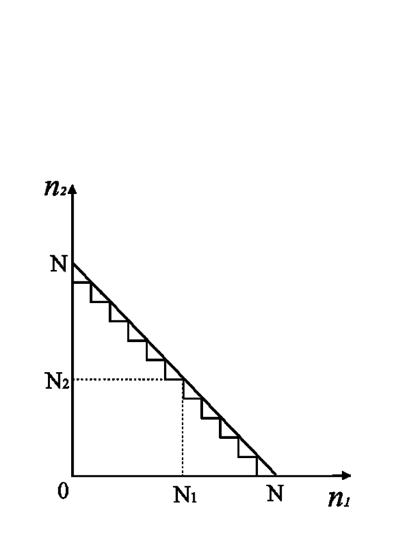
Figure 4: $\bar{D}$ : $N_{1}+N_{2}=N$ determined the set of intermediate states $\bar{D}$. It is used for the definition of the trace operation.

With these initial (or final) states, we define trace operation with boundary as

$$Tr_{N}\Psi^{\dagger}O\Psi \equiv tr\sum_{all\ \langle initial|}\langle initial|\Psi^{\dagger}O\Psi|initial\rangle$$ (95)

$$= tr \!\!\!\!\!\!\!\sum_{\scriptsize\begin{array}[]{c}n_{1}+n_{2}\leq N\\ n_{1}^{\prime}+n_{2}^{\prime}\leq N\end{array}}\sum_{all\ \langle initial|}\langle n_{1},n_{2}|O|n_{1}^{\prime},n_{2}^{\prime}\rangle\langle n_{1},n_{2}|\Psi|initial\rangle\langle initial|\Psi^{\dagger}|n_{1}^{\prime},n_{2}^{\prime}\rangle,$$ (98)

where $tr$ denotes trace of any other kind of indices without Fock space, that is the trace of $(2k+n)\times(2k+n)$ dimension matrices or gauge group U(n). Here, it is worth to emphasize the merit of definition (92) and (95). In the computation of the Pontrjagin class, ${\cal D}\Psi|initial\rangle$ or $\langle final|\Psi^{\dagger}{\cal D}^{\dagger}$ often appear. If there is no boundary, then the zero mode $\Psi$ satisfies ${\cal D}\Psi=0$ by definition. However, we have boundary and the Fock space is finite, then the condition is not satisfied on the boundary in general. Because the operator ${\cal D}$ includes creation and annihilation operators, cancellation of each state is occurred by chain reaction. On the boundary, the chain of cancellation is broken. For example, if we choose (92) as the domain and $N_{1}+N_{2}=N$ as boundary of intermediate state , following non-vanishing terms remain:

$$\sum_{all\ |initial\rangle}{\cal D}\Psi|initial\rangle = \sum_{all\ |initial\rangle}\ \sum_{N_{1}+N_{2}=N}{\cal D}_{b}|N_{1},N_{2}\rangle 1_{[2k+n]}\langle N_{1},N_{2}|\Psi|initial\rangle$$

$$=\sum_{all\ |initial\rangle}\ \sum_{N_{1}+N_{2}=N} \!\!\!\!\!\!\!\!\!\!\!\!\left(\begin{array}[]{ccc}-\sqrt{\zeta}c_{2}^{\dagger}&-\sqrt{\zeta}c_{1}^{\dagger}&0\\ -B_{1}^{\dagger}&B_{2}^{\dagger}&J^{\dagger}\end{array}\right)|N_{1},N_{2}\rangle 1_{[2k+n]}\langle N_{1},N_{2}|\Psi|initial\rangle.$$ (101)

Here ${\cal D}_{b}$ denotes a operator whose operands are boundary states of intermediate state (in this case, intermediate state belong to $\bar{D}$) and it is expressed as

$$\sum_{(n_{1},n_{2})\in domain}\!\!\!\!\!\!\!\!\!\!{\cal D}|n_{1},n_{2}\rangle 1_{[2k+n]}\langle n_{1},n_{2}|\Psi=\!\!\!\!\!\!\!\!\!\!\sum_{(N_{1},N_{2})\in boundary}\!\!\!\!\!\!\!\!\!\!{\cal D}_{b}|N_{1},N_{2}\rangle 1_{[2k+n]}\langle N_{1},N_{2}|\Psi.$$ (102)

Using (101), we can perform the instanton charge calculation concretely and easily. This is the most important merit to introduce the boundary (92).

Note that the ${\cal D}_{b}$ do not have universal form for each intermediate boundary state. i.e. ${\cal D}\Psi$ on boundary is not always expressed by Eq.(101). As an example, let us study the case of

$$\sum_{all\ |initial\rangle}{\cal D}\Psi\Psi^{\dagger}c_{\alpha}\Psi|initial\rangle.$$ (103)

If there is no boundary, ${\cal D}\Psi\Psi^{\dagger}$ is zero by the definition of the zero-mode $\Psi$. But in (103), there is boundary at $\Psi|initial\rangle$ with the definition (92). Then $\Psi\Psi^{\dagger}c_{\alpha}\Psi|initial\rangle$ is also expanded by finite number of the basis of the Fock space, and there is intermediate boundary. In this case, intermediate state $|inter\rangle$ is defined by complete system that can expand the space $\{\Psi\Psi^{\dagger}c_{\alpha}\Psi|initial\rangle\}$, and its $i$-component $|inter\ (i)\rangle$ satisfies

$${}^{\exists}|initial\rangle : \sum_{j}\langle inter\ (i)|(\Psi\Psi^{\dagger}c_{\alpha}\Psi)_{ij}|initial\ (j)\rangle\neq 0.$$ (104)

We call set of the finite number of intermediate states $\bar{I}$ i.e. $\bar{I}=\{|inter\rangle\}$ . Then the boundary $|{\bf int.\!\!\!-b(i)}\rangle$ of the intermediate state is defined by

$$|{\bf int.\!\!\!-b(i)}\rangle \equiv b_{n_{1},n_{2},i}|n_{1}^{(i)},n_{2}^{(i)}\rangle$$ (105)

$$\big{(}{}^{\exists}\langle inter\ (i)| : \langle inter\ (i)|n_{1}^{(i)},n_{2}^{(i)}\rangle\neq 0\big{)},$$ (109)

$${\rm and} \left\{\begin{array}[]{c}\big{(}{}^{\forall}\langle inter\ (i)|:\langle inter\ (i)|n_{1}^{(i)}+1,n_{2}^{(i)}\rangle=0\big{)}\\ \ {\rm or}\\ \big{(}{}^{\forall}\langle inter\ (i)|:\langle inter\ (i)|n_{1}^{(i)},n_{2}^{(i)}+1\rangle=0\big{)}\end{array}\right\}.$$

For any $|initial\rangle$,

$${\cal D}\Psi\Psi^{\dagger}c_{\alpha}\Psi|initial\rangle = \sum_{{\bf int.\!\!\!-b}}{\cal D}_{b}|{\bf int.\!\!\!-b}\rangle\langle{\bf int.\!\!\!-b}|\Psi\Psi^{\dagger}c_{\alpha}\Psi|initial\rangle\ .$$ (110)

We have to pay attention to the point that this intermediate boundary is not possible to be expressed by the simple one condition like $N_{1}+N_{2}=N$ in (101), since $\Psi\Psi^{\dagger}c_{\alpha}$ make the boundary be complex. So we can not express the explicit expression of the ${\cal D}_{b}|{\bf int.\!\!\!-b}\rangle$. Fortunately, we do not need its explicit expression in the calculation of the instanton charge in the next subsection, since the leading terms contributing to the instanton charge have lower exponent of $N$ than the the case of (101). For the convenience of the next subsection, we estimate the behavior of ${\cal D}\Psi\Psi^{\dagger}c_{\alpha}\Psi|initial\rangle$ near the boundary. As a result of ${\cal D}\Psi=0$, the order estimation of $\Psi$ near the boundary give us

$$\Psi\sim\left(\begin{array}[]{c}\frac{1}{\sqrt{N}}\\ \frac{1}{\sqrt{N}}\\ 1\end{array}\right)\ \begin{array}[]{c}\}k\\ \}k\\ \}n\end{array}\ .$$ (117)

Using this and (78), the non-vanishing leading term of ${\cal D}\Psi\Psi^{\dagger}c_{\alpha}\Psi$ for a some state $|N_{1},N_{2}\rangle$ near boundary $N_{1}+N_{2}=N$ is

$${\cal D} \!\!\!\!\!\!\!\!\Psi\Psi^{\dagger}c_{\alpha}|N_{1},N_{2}\rangle 1_{[2k+n]}\langle N_{1},N_{2}|\Psi|initial\rangle\sim$$ (121)

$$\left(\begin{array}[]{c}\{B_{2}(Ic_{2}\frac{1}{N}-J^{\dagger}c^{\dagger}_{1}\frac{1}{N})c_{\alpha}+B_{1}(Ic_{1}\frac{1}{N}+J^{\dagger}c^{\dagger}_{2}\frac{1}{N})c_{\alpha}\}|N_{1},N_{2}\rangle\\ \{-B_{1}^{\dagger}(Ic_{2}\frac{1}{N}-J^{\dagger}c^{\dagger}_{1}\frac{1}{N})c_{\alpha}+B_{2}^{\dagger}(Ic_{1}\frac{1}{N}+J^{\dagger}c^{\dagger}_{2}\frac{1}{N})c_{\alpha}\}|N_{1},N_{2}\rangle\end{array}\right).$$

Leading terms cancel each other, then only next leading terms remain in (121). Therefore we can see this expression is not similar to Eq.(101) at all. The terms like this appear in the integral of the Pontrjagin class in the next subsection, but it is shown by order estimation of $N$ that such terms do not contribute to the integral.

For later computation, it is useful to emphasize one fact that for arbitrary operand state in $\underline{{\it D}}$ we do not have to distinguish the projector $\Psi\Psi^{\dagger}$ from $\sum\Psi|n_{1},n_{2}\rangle\langle n_{1},n_{2}|\Psi^{\dagger}$ whose region of the summation is some set of intermediate states like $\bar{I}$ or $\bar{D}$. This fact is obtained from the Remark3.0.2 and the definition of the boundary. The Remark3.0.2 shows that the $v_{0}$ have almost no element near the boundary for large $N$, then $\Psi$ is an isometry from finite domain $\underline{{\it D}}$ to $\bar{D}$, and $|\langle n,m|\Psi|n^{\prime},m^{\prime}\rangle|$ is almost zero if $(n,m)\not{\!\!\in}\bar{D}$ and $(n^{\prime},m^{\prime})\in\underline{{\it D}}$. This is why we do not have to distinguish $\Psi\Psi^{\dagger}$ from $\sum\Psi|n_{1},n_{2}\rangle\langle n_{1},n_{2}|\Psi^{\dagger}$.

At the last of this subsection, we emphasize that the result of the calculation is independent from the choice of boundary. We chose artificial boundary in this section to make calculation be simple. But, if we perform the same calculation by commutative fields with using the star product (see for example [4]), it is easy to understand that choosing boundary do not change the result. So far as the instanton charge is well-defined by converge series, the result is identified with the result using the star product calculation. Indeed in the next subsection, essentially we use only the fact that the boundary states have large eigenvalue of total number operator $N$ and the rank of the boundary states (number of the Fock state that construct the boundary) is $O\!(N)$. (But the notation and calculation change into simple one as a result of the definition (92).) So, all we have to do is to make sure that the series is converge and identified with the instaton number that appear in ADHM construction as a dimension of vector space.

4.2 Direct calculation of Instanton charge

Let us carry out the calculation of the instanton charge with only primitive methods. Using boundary, $D_{\alpha}$ and (21) the instanton charge (the integral of the first Pontrjagin class) is written as

$$Q = \lim_{N\rightarrow\infty}Q_{N}$$ (122)

$$Q_{N} = -\mbox{Tr}_{N}1+\frac{\zeta^{2}}{2}\mbox{Tr}_{N}\left\{[D_{1},D_{\bar{1}}][D_{2},D_{\bar{2}}]+[D_{2},D_{\bar{2}}][D_{1},D_{\bar{1}}]\right.$$

$$\left.\hskip 71.13188pt-[D_{1},D_{\bar{2}}][D_{2},D_{\bar{1}}]-[D_{2},D_{\bar{1}}][D_{1},D_{\bar{2}}]\right\}$$

$$= -\mbox{Tr}_{N}1+\frac{\zeta^{2}}{2}\mbox{Tr}_{N}\left\{[D_{\bar{2}},\ D_{2}D_{\bar{1}}D_{1}-D_{1}D_{\bar{1}}D_{2}]+[D_{\bar{1}},\ D_{1}D_{\bar{2}}D_{2}-D_{2}D_{\bar{2}}D_{1}]\right\}.$$

The boundary that we use is defined by (101) in the previous subsection.

Let us see the concrete form of these terms. Note that ${\cal D}\Psi\neq 0$ because our calculation is done with boundary, as we studied in the previous subsection. The surviving terms that contain ${\cal D}\Psi$ proportional terms exist on the boundary. So we can use the Eqs.(101),(121) and so on, for these surviving terms. Using (78), (83-88) and commutation relations, we get following explicit expression.
$D_{2}D_{\bar{1}}D_{1}$ :

$$\zeta^{\frac{3}{2}} \!\!\!\!\!D_{2}D_{\bar{1}}D_{1}=$$ (130)

$$- \Psi^{\dagger}c_{2}n_{1}\Psi$$

$$+ \Psi^{\dagger}{\cal D}^{\dagger}c_{2}\frac{1}{{\cal D}{\cal D}^{\dagger}}n_{1}{\cal D}\Psi$$

$$+ \Psi^{\dagger}\left(\begin{array}[]{ccc}0&0&0\\ -\zeta\frac{1}{\square}c_{1}&0&0\\ 0&0&0\end{array}\right)\Psi+\Psi^{\dagger}\left(\begin{array}[]{ccc}0&0&0\\ 0&\zeta c_{2}\frac{1}{\square}&0\\ 0&0&0\end{array}\right)\Psi$$

$$+ \Psi^{\dagger}\tau^{\dagger}c_{2}\frac{1}{\square}(0,\sqrt{\zeta}c_{1}^{\dagger},0)\Psi+\Psi^{\dagger}\sigma c_{2}\frac{1}{\square}(\sqrt{\zeta}c_{1},0,0)\Psi+\Psi^{\dagger}\left(\begin{array}[]{c}0\\ -\sqrt{\zeta}\\ 0\end{array}\right)\frac{1}{\square}n_{1}\sigma^{\dagger}\Psi$$ (134)

$$+ \Psi^{\dagger}\left(\begin{array}[]{c}0\\ \sqrt{\zeta}\\ 0\end{array}\right)c_{2}\frac{1}{\square}c_{1}\tau\Psi$$ (138)

$$- \Psi^{\dagger}{\cal D}^{\dagger}c_{2}\frac{1}{{\cal D}{\cal D}^{\dagger}}{\cal D}\left(\begin{array}[]{c}0\\ \sqrt{\zeta}\\ 0\end{array}\right)\frac{1}{\square}c_{1}\tau\Psi\ .$$ (142)

$D_{1}D_{\bar{1}}D_{2}$:

$$\zeta^{\frac{3}{2}} \!\!\!\!\!D_{1}D_{\bar{1}}D_{2}=$$ (149)

$$- \Psi^{\dagger}c_{1}c_{1}^{\dagger}c_{2}\Psi$$

$$+ \Psi^{\dagger}{\cal D}^{\dagger}(n_{1}+1)\frac{1}{{\cal D}{\cal D}^{\dagger}}c_{2}{\cal D}\Psi$$

$$+ \Psi^{\dagger}\left(\begin{array}[]{ccc}\zeta\frac{1}{\square}c_{2}&0&0\\ 0&0&0\\ 0&0&0\end{array}\right)\Psi+\Psi^{\dagger}\left(\begin{array}[]{ccc}0&0&0\\ \zeta c_{1}\frac{1}{\square}&0&0\\ 0&0&0\end{array}\right)\Psi$$

$$+ \Psi^{\dagger}\tau^{\dagger}(n_{1}+1)\frac{1}{\square}(\sqrt{\zeta},0,0)\Psi+\Psi^{\dagger}\left(\begin{array}[]{c}0\\ \sqrt{\zeta}c_{1}\\ 0\end{array}\right)\frac{1}{\square}c_{2}\tau\Psi$$ (153)

$$+ \Psi^{\dagger}\left(\begin{array}[]{c}\sqrt{\zeta}c_{1}^{\dagger}\\ 0\\ 0\end{array}\right)\frac{1}{\square}c_{2}\sigma^{\dagger}\Psi+\Psi^{\dagger}\sigma c_{1}\frac{1}{\square}(\sqrt{\zeta}c_{2},0,0)$$ (157)

$$- \Psi^{\dagger}\sigma c_{1}\frac{1}{\square}(\sqrt{\zeta},0,0){\cal D}^{\dagger}\frac{1}{{\cal D}{\cal D}^{\dagger}}c_{2}{\cal D}\Psi\ .$$ (158)

Note that the matrices sandwiched between $\Psi^{\dagger}$ and $\Psi$ are $(k+k+n)\times(k+k+n)$ matrices. Here we ignore low order terms of $N$ that do not contribute to the instanton charge. For example,

$$\Psi^{\dagger}{\cal D}^{\dagger}c_{2}({\cal D}{\cal D}^{\dagger})^{-1}{\cal D}\left(\begin{array}[]{ccc}0&0&0\\ 0&\zeta\frac{1}{\square}&0\\ 0&0&0\end{array}\right)\Psi=\Psi^{\dagger}\left.\left(\begin{array}[]{ccc}0&o(\frac{N_{2}}{N})&0\\ 0&O(\frac{N_{2}}{N})&0\\ 0&o(\frac{N_{2}}{N})&0\end{array}\right)\Psi\right|_{boundary}$$ (165)

is removed from (142). Because its contribution to the instanton charge is

$$\lim_{N\rightarrow\infty} \!\!\!\!\!\!\!\!\!\!Tr_{N}\Big{[}\Psi^{\dagger}c_{2}\Psi\ ,\ \Psi^{\dagger}\left(\begin{array}[]{ccc}0&o(\frac{\sqrt{N_{2}}}{N})&0\\ 0&O(\frac{\sqrt{N_{2}}}{N})&0\\ 0&o(\frac{\sqrt{N_{2}}}{N})&0\end{array}\right)\Psi\Big{]}\sim\lim_{N\rightarrow\infty}\sum_{boundary}O\left(\frac{1}{N^{\frac{3}{2}}}\right)$$ (169)

$$\sim \lim_{N\rightarrow\infty}N\ O\!\left(N^{-\frac{3}{2}}\right)=0,$$ (170)

where $\sum_{boundary}$ denotes the trace over the boundary constructed out of $N$ Fock states. Explicit expression (83-88) is used here.

Using (142) and (158),

$$Q_{N} = -Tr_{N}1+\frac{\zeta^{\frac{3}{2}}}{2}\left\{Tr_{N}[\Psi^{\dagger}c_{2}^{\dagger}\Psi\ ,\ D_{2}D_{\bar{1}}D_{1}-D_{1}D_{\bar{1}}D_{2}]+(1\iff 2)\right\}$$ (171)

$$= -Tr_{N}1+\frac{1}{2}\left\{Tr_{N}(A_{1}+A_{2}+A_{3}+A_{4})+(1\iff 2)\right\},$$

where $(1\iff 2)$ is defined by $f(z_{1},z_{2})-(1\iff 2)\equiv f(z_{1},z_{2})-f(z_{2},z_{1})$, and $A_{1},A_{2},A_{3}$ and $A_{4}$ are defined by

$$A_{1} = [\Psi^{\dagger}c_{2}^{\dagger}\Psi\ ,\ -\Psi^{\dagger}c_{2}n_{1}\Psi+\Psi^{\dagger}c_{1}c_{1}^{\dagger}c_{2}\Psi]=[\Psi^{\dagger}c_{2}^{\dagger}\Psi\ ,\ \Psi^{\dagger}c_{2}\Psi]$$ (172)

$$A_{2} = \left[\Psi^{\dagger}c_{2}^{\dagger}\Psi\ ,\ \Psi^{\dagger}\left(\begin{array}[]{ccc}0&0&0\\ -\zeta\frac{1}{\square}c_{1}&0&0\\ 0&0&0\end{array}\right)\Psi+\Psi^{\dagger}\left(\begin{array}[]{ccc}0&0&0\\ 0&\zeta c_{2}\frac{1}{\square}&0\\ 0&0&0\end{array}\right)\Psi\right]$$ (186)

$$-\left[\Psi^{\dagger}c_{2}^{\dagger}\Psi\ ,\ \Psi^{\dagger}\left(\begin{array}[]{ccc}\zeta\frac{1}{\square}c_{2}&0&0\\ 0&0&0\\ 0&0&0\end{array}\right)\Psi+\Psi^{\dagger}\left(\begin{array}[]{ccc}0&0&0\\ \zeta c_{1}\frac{1}{\square}&0&0\\ 0&0&0\end{array}\right)\Psi\right]$$

$$= \left[\Psi^{\dagger}c_{2}^{\dagger}\Psi\ ,\ \Psi^{\dagger}\left(\begin{array}[]{ccc}-\zeta\frac{1}{\square}c_{2}&0&0\\ -\zeta c_{1}\frac{2}{\square}&\zeta c_{2}\frac{1}{\square}&0\\ 0&0&0\end{array}\right)\Psi\right]$$ (190)

$$A_{3} = \left[\Psi^{\dagger}c_{2}^{\dagger}\Psi\ ,\ \Psi^{\dagger}{\cal D}^{\dagger}c_{2}\frac{1}{{\cal D}{\cal D}^{\dagger}}n_{1}{\cal D}\Psi-\Psi^{\dagger}{\cal D}^{\dagger}c_{2}\frac{1}{{\cal D}{\cal D}^{\dagger}}{\cal D}\left(\begin{array}[]{c}0\\ \sqrt{\zeta}\\ 0\end{array}\right)\frac{1}{\square}c_{1}\tau\Psi\right]$$

$$- \left[\Psi^{\dagger}c_{2}^{\dagger}\Psi\ ,\ \Psi^{\dagger}{\cal D}^{\dagger}(n_{1}+1)\frac{1}{{\cal D}{\cal D}^{\dagger}}c_{2}{\cal D}\Psi-\Psi^{\dagger}\sigma c_{1}\frac{1}{\square}(\sqrt{\zeta},0,0){\cal D}^{\dagger}\frac{1}{{\cal D}{\cal D}^{\dagger}}c_{2}{\cal D}\Psi\right]$$

$$A_{4} = \left[\Psi^{\dagger}c_{2}^{\dagger}\Psi\ ,\ \Psi^{\dagger}\tau^{\dagger}c_{2}\frac{1}{\square}(0,\sqrt{\zeta}c_{1}^{\dagger},0)\Psi+\Psi^{\dagger}\sigma c_{2}\frac{1}{\square}(\sqrt{\zeta}c_{1},0,0)\Psi\right.$$ (209)

$$\ \ \ \ \ \ \ \ \ \ \ \ \ \ \ \ \left.+\Psi^{\dagger}\left(\begin{array}[]{c}0\\ -\sqrt{\zeta}\\ 0\end{array}\right)\frac{1}{\square}n_{1}\sigma^{\dagger}\Psi+\Psi^{\dagger}\left(\begin{array}[]{c}0\\ \sqrt{\zeta}\\ 0\end{array}\right)c_{2}\frac{1}{\square}c_{1}\tau\Psi\right]$$

$$-\left[\Psi^{\dagger}c_{2}^{\dagger}\Psi\ ,\ \Psi^{\dagger}\tau^{\dagger}(n_{1}+1)\frac{1}{\square}(\sqrt{\zeta},0,0)\Psi+\Psi^{\dagger}\left(\begin{array}[]{c}0\\ \sqrt{\zeta}c_{1}\\ 0\end{array}\right)\frac{1}{\square}c_{2}\tau\Psi\right.$$

$$\ \ \ \ \ \ \ \ \ \ \ \ \ \ \ \ \left.+\Psi^{\dagger}\left(\begin{array}[]{c}\sqrt{\zeta}c_{1}^{\dagger}\\ 0\\ 0\end{array}\right)\frac{1}{\square}c_{2}\sigma^{\dagger}\Psi+\Psi^{\dagger}\sigma c_{1}\frac{1}{\square}(\sqrt{\zeta}c_{2},0,0)\right].$$

$A_{3}$ has intermidiate boundary whose states are operated by ${\cal D}$ or $\tau$ or $\sigma$, like (103). From (121), the trace of $A_{3}$ is estimated as

$$\lim_{N\rightarrow\infty}Tr_{N}A_{3}\leq C\lim_{N\rightarrow\infty}N\ O\!\left(N^{-\frac{3}{2}}\right)=0,$$ (210)

where $C$ is some constant.
On the other hand, $A_{4}$ is constructed from the commutation relation of the terms like $\Psi^{\dagger}{\cal D}^{\dagger}\cdots\Psi$ or $\Psi^{\dagger}\cdots{\cal D}\Psi$. The trace of such terms is

$$Tr_{N} \!\!\!\!\!\!\!\left[\Psi^{\dagger}c_{2}^{\dagger}\Psi\ ,\ \Psi^{\dagger}{\cal D}^{\dagger}\cdots\Psi\right]$$

$$= tr\!\!\!\!\!\!\!\sum_{{\bf all}\ |initial\rangle}\left\{\langle initial|\Psi^{\dagger}c_{2}^{\dagger}\Psi\Psi^{\dagger}\sum_{{\bf all}\ {\bf int.\!\!\!-b}}|{\bf int.\!\!\!-b}\rangle\langle{\bf int.\!\!\!-b}|{\cal D}^{\dagger}_{b}\cdots\Psi|initial\rangle\right.$$

$$\left.-\langle initial|\Psi^{\dagger}\sum_{N_{1}+N_{2}=N}|N_{1},N_{2}\rangle\langle N_{1},N_{2}|{\cal D}^{\dagger}\cdots\Psi\Psi^{\dagger}c_{2}^{\dagger}\Psi|initial\rangle\right\}$$

$$= N\ O\!\left(N^{-\frac{3}{2}}\right)-Tr_{N}\left\{\Psi^{\dagger}\!\!\!\!\sum_{N_{1}+N_{2}=N}|N_{1},N_{2}\rangle\langle N_{1},N_{2}|{\cal D}_{b}^{\dagger}\cdots\Psi\Psi^{\dagger}c_{2}^{\dagger}\Psi\right\}.$$ (212)

Therefore trace of $A_{4}$ is

$$Tr_{N}A_{4} = O\!\left(N^{-\frac{1}{2}}\right)+$$ (213)

$$tr\!\!\!\!\!\!\!\sum_{{\bf all}\ |initial\rangle} \!\!\!\!\!\!\!\!\!\!\!\!\!\!\!\!\!\!\!\!\ \!\!\!\!\!\!\!\ \langle initial|\left\{\Psi^{\dagger}\!\!\!\!\!\!\sum_{N_{1}+N_{2}=N}\!\!\!\!\!\!|N_{1},N_{2}\rangle\langle N_{1},N_{2}|\left(\begin{array}[]{ccc}\zeta c_{2}\frac{N_{1}}{N}&-\zeta c_{2}{}^{2}\frac{1}{N}c_{1}^{\dagger}&0\\ \zeta\frac{N_{1}}{N}c_{1}&-\zeta c_{2}\frac{N_{1}}{N}c_{1}^{\dagger}&0\\ 0&0&0\end{array}\right)\Psi\Psi^{\dagger}c_{2}^{\dagger}\Psi\right.$$ (217)

$$-\Psi^{\dagger}c_{2}^{\dagger}\!\!\!\!\! \Psi\Psi^{\dagger} \!\!\!\!\!\left.\left(\begin{array}[]{ccc}0&0&-\sqrt{\zeta}c_{1}^{\dagger}\frac{1}{N}c_{2}J^{\dagger}\\ 0&0&-\sqrt{\zeta}\frac{N_{1}}{N}J^{\dagger}\\ 0&0&0\end{array}\right)\!\!\!\sum_{N_{1}+N_{2}=N}\!\!\!\!\!|N_{1},N_{2}\rangle\langle N_{1},N_{2}|\Psi\right\}|initial\rangle.$$ (221)

Near the boundary ($N_{1}+N_{2}=N$) we can use concrete form of $\Psi\Psi^{\dagger}$ (78), then it is shown that the last two terms vanish. After all,

$$\lim_{N\rightarrow\infty}Tr_{N}A_{4}=\lim_{N\rightarrow\infty}O\!\left(N^{-\frac{1}{2}}\right)=0.$$ (222)

From Eqs.(210) and (222), we can understand the survived terms are obtained from $A_{1}$ and $A_{2}$. In the previous discussion about $A_{3}$ and $A_{4}$, ${\cal D}\Psi$ appeared and it made the trace operation be a summation over the boundary. On the other hand, $A_{1}$ and $A_{2}$ do not have such terms, then we have to calculate $A_{1}$ and $A_{2}$ by another method. It is Stokes’ like theorem. For some operator $\Psi^{\dagger}O\Psi=\sum O_{l_{1},p_{1},l_{2},p_{2}}\Psi^{\dagger}|l_{1},p_{1}\rangle\langle l_{2},p_{2}|\Psi$, commutation relation with $D_{\bar{2}}$ is given as follows,

$$Tr_{N}[\Psi^{\dagger}c_{2}^{\dagger}\Psi \Psi^{\dagger}O\Psi]$$ ,

$$=\!\!\!\!\!\!\!\!\!\!\sum_{\scriptsize\begin{array}[]{c}n_{1},m_{1}\in D\\ n_{2},m_{2}\in I\end{array}}\!\!\!\!\!\sum_{\scriptsize\begin{array}[]{c}l_{3},p_{3}\in\bar{D}\\ l_{2},p_{2}\in\bar{I}\end{array}} \!\!\!\!\!\!\!\!\!\!\sum_{l_{1},p_{1}\in\bar{D}}\Psi^{\dagger}_{n_{1},m_{1},l_{1},p_{1}}\sqrt{p_{1}}\Psi_{l_{1},p_{1}-1,n_{2},m_{2}}\Psi^{\dagger}_{n_{2},m_{2},l_{2},p_{2}}O_{l_{2},p_{2},l_{3},p_{3}}\Psi_{l_{3},p_{3},n_{1},m_{1}}$$ (227)

$$-\!\!\!\!\!\!\!\!\!\!\sum_{\scriptsize\begin{array}[]{c}n_{1},m_{1}\in D\\ n_{2},m_{2}\in I\end{array}}\!\!\!\!\sum_{\scriptsize\begin{array}[]{c}l_{3},p_{3}\in c_{2}^{\dagger}\bar{D}\\ l_{2},p_{2}\in c_{2}^{\dagger}\bar{I}\end{array}} \!\!\!\!\!\!\!\!\!\!\!\sum_{l_{1},p_{1}\in\bar{D}}\Psi^{\dagger}_{n_{1},m_{1},l_{1},p_{1}}O_{l_{1},p_{1},l_{2},p_{2}}\Psi_{l_{2},p_{2},n_{2},m_{2}}\Psi^{\dagger}_{n_{2},m_{2},l_{3},p_{3}}\sqrt{p_{3}}\Psi_{l_{3},p_{3}-1,n_{1},m_{1}}$$ (232)

$$=\!\!\!\!\!\!\!\sum_{\scriptsize\begin{array}[]{c}l_{1},p_{1}\in\bar{D}\\ l_{3},p_{3}\in\bar{D}\end{array}} \!\!\!\!\!\!\!\!\!\!\sum_{l_{2},p_{2}\in\bar{D}}(\Psi\Psi^{\dagger})_{l_{3},p_{3},l_{1},p_{1}}\sqrt{p_{1}}(\Psi\Psi^{\dagger})_{l_{1},p_{1}-1,l_{2},p_{2}}O_{l_{2},p_{2},l_{3},p_{3}}$$ (235)

$$-\!\!\!\!\!\!\!\sum_{\scriptsize\begin{array}[]{c}l_{2},p_{2}\in c_{2}^{\dagger}\bar{D}\\ l_{3},p_{3}\in c_{2}^{\dagger}\bar{D}\end{array}} \!\!\!\!\!\!\!\!\!\!\sum_{l_{1},p_{1}\in\bar{D}}(\Psi\Psi^{\dagger})_{l_{2},p_{2},l_{3},p_{3}}\sqrt{p_{3}}(\Psi\Psi^{\dagger})_{l_{3},p_{3}-1,l_{1},p_{1}}O_{l_{1},p_{1},l_{2},p_{2}},$$ (238)

where $c_{2}^{\dagger}\bar{D}$ $(c_{2}^{\dagger}\bar{I})$ is domain defined by $\bar{D}$ $(\bar{I})$ shifted by $c_{2}^{\dagger}$ (see Fig.5). Here we omit the indices of $2k+n$ dimension vector for simplicity. The domain of the trace operation $\bar{D}$ is universal among each component of $2k+n$ dimension vector by the definition of the boundary in the previous subsection (92) and (95). On the other hand, for intermediate state there is no universal domain, i.e. the integral domain of intermediate states is determined case by case. So the $I$ and $\bar{I}$ are only symbolical character that means domain of the intermediate states.
Only the terms that are on the boundary shifted by $c_{2}^{\dagger}$ are remained because they have no partner to cancel out.

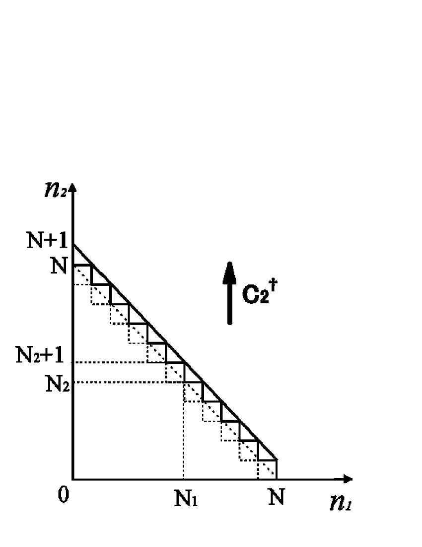
Figure 5: $c_{2}^{\dagger}\bar{D}$ : $c_{2}^{\dagger}\bar{D}$ is defined by $\bar{D}$ shifted by $c_{2}^{\dagger}$. Trace over its boundary contribute to the instanton charge.

Then the remaining terms are written as

$$-\!\!\!\!\!\sum_{\scriptsize\begin{array}[]{c}l_{2},p_{2}\in\bar{D}\\ l_{3},p_{3}\in c_{2}^{\dagger}\bar{D}\end{array}} \!\!\!\!\!\!\!\!\!\!\sum_{N_{1}+N_{2}=N}\!\!\!\!\!\!\sqrt{N_{2}+1}(\Psi\Psi^{\dagger})_{N_{1},N_{2},l_{2},p_{2}}O_{l_{2},p_{2},l_{3},p_{3}}(\Psi\Psi^{\dagger})_{l_{3},p_{3}-1,N_{1},N_{2}+1}$$ (241)

$$-\!\!\!\!\!\sum_{\scriptsize\begin{array}[]{c}l_{1},p_{1}\in\bar{D}\\ l_{3},p_{3}\in\bar{D}\end{array}} \!\!\!\!\!\!\!\!\!\!\sum_{N_{1}+N_{2}=N}(\Psi\Psi^{\dagger})_{N_{1},N_{2}+1,l_{3},p_{3}}\sqrt{p_{3}}(\Psi\Psi^{\dagger})_{l_{3},p_{3}-1,l_{1},p_{1}}O_{l_{1},p_{1},N_{1},N_{2}+1}.$$ (244)

Using this result, let us investigate $A_{2}$ terms here. To adapt (241) and (244) for $A_{2}$, $O$ should be replaced by

$$\left(\begin{array}[]{ccc}-\zeta\frac{1}{\square}c_{2}&0&0\\ -\zeta c_{1}\frac{2}{\square}&\zeta c_{2}\frac{1}{\square}&0\\ 0&0&0\end{array}\right).$$ (248)

It is better for simplicity, that (241) and (244) are evaluated separately. As a result of the definition of the boundary, only non-vanishing term in (241) is given as

$$-Tr_{\scriptsize boundary} \left\{c_{2}^{\dagger}\left(\begin{array}[]{ccc}\cdots&\cdots&\vdots\\ \cdots&\cdots&\vdots\\ I^{\dagger}\frac{1}{\sqrt{\zeta}N}c_{2}^{\dagger}&I^{\dagger}\frac{1}{\sqrt{\zeta}N}c_{1}^{\dagger}&\ddots\end{array}\right)\left(\begin{array}[]{ccc}-\zeta\frac{1}{\square}c_{2}&0&0\\ -\zeta c_{1}\frac{2}{\square}&\zeta c_{2}\frac{1}{\square}&0\\ 0&0&0\end{array}\right)\right.$$ (259)

$$\left.\times\left(\begin{array}[]{ccc}\cdots&\cdots&c_{2}\frac{1}{\sqrt{\zeta}N}I\\ \cdots&\cdots&c_{1}\frac{1}{\sqrt{\zeta}N}I\\ \cdots&\cdots&\ddots\end{array}\right)\right\}$$

$$= \frac{1}{\zeta}tr\sum_{boundary}I^{\dagger}\frac{N_{2}}{N}I$$ (260)

Here $Tr_{boundary}$ denotes a summation over the boundary of $c_{2}^{\dagger}\bar{D}$ and we ignore some components that do not contribute to the integral in the large $N$ limit. $tr$ represent trace operation for the all indices without Fock space indices i.e. $\makebox{tr}_{U(N)}$.

Let us evaluate (244) in $A_{2}$. As a result of the boundary definition, we can conclude that $\langle l_{3},p_{3}-1|c_{2}^{\dagger}|N_{1},N_{2}\rangle=0$ if $(l_{3},p_{3}-1)\in\bar{D}$. Then (244) whose $O$ is replaced by (248) is

$$-tr\sum_{N_{1}+N_{2}=N} \left\{\langle N_{1},N_{2}|\frac{c_{2}}{\sqrt{N_{2}}}\left(\begin{array}[]{ccc}\cdots&\cdots&-\frac{1}{\sqrt{\zeta}N}c_{1}^{\dagger}J^{\dagger}\\ \cdots&\cdots&c_{2}^{\dagger}\frac{1}{\sqrt{\zeta}N}J^{\dagger}\\ I^{\dagger}\frac{1}{\sqrt{\zeta}N}c_{2}^{\dagger}&I^{\dagger}\frac{1}{\sqrt{\zeta}N}c_{1}^{\dagger}&1_{[n]}\end{array}\right)\right.$$ (264)

$$\times\!\!\! c_{2}^{\dagger} \!\!\!\!\!\left.\left(\begin{array}[]{ccc}\cdots&\cdots&0\\ \cdots&\cdots&0\\ -J\frac{\sqrt{(N_{2}+1)}}{\sqrt{\zeta}N^{2}}c_{1}&I^{\dagger}\frac{\sqrt{(N_{2}+1)}}{\sqrt{\zeta}N^{2}}c_{1}^{\dagger}+J\frac{\sqrt{(N_{2}+1)}}{\sqrt{\zeta}N^{2}}c_{2}&0\end{array}\right)|N_{1},N_{2}\rangle\right\}$$ (268)

$$= -\frac{1}{\zeta}\ tr\sum_{boundary}\left(J\frac{N_{2}^{2}+N_{1}N_{2}}{N^{3}}J^{\dagger}\right),$$ (269)

where we use $tr(IJ)=-tr([B_{1},B_{2}])=0$. From (260) and (269),

$$Tr_{N}(A_{2}+(1\iff 2))=Tr_{boundary}\frac{1}{\zeta N}(I^{\dagger}I-JJ^{\dagger})$$

$$=\frac{1}{\zeta}tr(I^{\dagger}I-JJ^{\dagger})=2k.$$ (270)

Here we use trace of the real ADHM equation (23).

Final work we have to do is to evaluate $A_{1}$. Using (35) and commutation relations

$$A_{1} = -{\zeta}[D_{\bar{2}}\ ,\ D_{2}]$$ (271)

$$= -1$$ (281)

$$-\Psi^{\dagger}{\cal D}^{\dagger}c_{2}^{\dagger}\frac{1}{{\cal D}{\cal D}^{\dagger}}c_{2}{\cal D}\Psi+\Psi^{\dagger}{\cal D}^{\dagger}c_{2}\frac{1}{{\cal D}{\cal D}^{\dagger}}c_{2}^{\dagger}{\cal D}\Psi$$

$$-\Psi^{\dagger}\tau^{\dagger}c_{2}^{\dagger}\frac{1}{\square}(\sqrt{\zeta},0,0)\Psi-\Psi^{\dagger}\left(\begin{array}[]{c}\sqrt{\zeta}\\ 0\\ 0\end{array}\right)\frac{1}{\square}c_{2}\tau\Psi$$

$$+\Psi^{\dagger}\sigma c_{2}\frac{1}{\square}(0,-\sqrt{\zeta},0)\Psi+\Psi^{\dagger}\left(\begin{array}[]{c}0\\ -\sqrt{\zeta}\\ 0\end{array}\right)\frac{1}{\square}c_{2}^{\dagger}\sigma^{\dagger}\Psi$$

$$- \!\!\!\!\Psi^{\dagger}\left(\begin{array}[]{c}\sqrt{\zeta}\\ 0\\ 0\end{array}\right)\frac{1}{\square}(\sqrt{\zeta},0,0)\Psi+\Psi^{\dagger}\left(\begin{array}[]{c}0\\ \sqrt{\zeta}\\ 0\end{array}\right)\frac{1}{\square}(0,\sqrt{\zeta},0)\Psi$$ (288)

Trace of (281) is represented as follows:

$$Tr_{N} \!\!\!\!\!\!\!\left\{-\Psi^{\dagger}{\cal D}_{b}^{\dagger}c_{2}^{\dagger}\frac{1}{{\cal D}{\cal D}^{\dagger}}c_{2}{\cal D}_{b}\Psi+\Psi^{\dagger}{\cal D}_{b}^{\dagger}c_{2}\frac{1}{{\cal D}{\cal D}^{\dagger}}c_{2}^{\dagger}{\cal D}_{b}\Psi\right\}$$

$$=Tr_{N} \!\!\!\!\!\!\!\!\left\{\Psi\left(\begin{array}[]{cc}-\sqrt{\zeta}c_{2}&-B_{1}\\ -\sqrt{\zeta}c_{1}&B_{2}\\ 0&J\end{array}\right)\left(\begin{array}[]{cc}c_{2}\frac{1}{\square}c_{2}^{\dagger}-c_{2}^{\dagger}\frac{1}{\square}c_{2}&0\\ 0&c_{2}\frac{1}{\square}c_{2}^{\dagger}-c_{2}^{\dagger}\frac{1}{\square}c_{2}\end{array}\right)\right.$$ (297)

$$\times\left.\left(\begin{array}[]{ccc}-\sqrt{\zeta}c_{2}^{\dagger}&-\sqrt{\zeta}c_{1}^{\dagger}&0\\ -B_{1}^{\dagger}&B_{2}^{\dagger}&J^{\dagger}\end{array}\right)\Psi\right\}.$$

After straightforward calculation with using concrete form of $1/\square$ of (74), (297) become

$$Tr_{boundary} \!\!\!\!\!\!\left\{\left(-1+\frac{2N_{2}^{2}+2N_{1}N_{2}}{N^{2}}\right)\left(\frac{1}{N}-\frac{1}{\zeta}II^{\dagger}\right)\right.$$ (298)

$$+ \frac{(N_{1}-N_{2})^{2}}{N^{3}}+\frac{-2N_{2}(N_{2}-N_{1})^{2}}{N^{4}}$$

$$+ 2\frac{N_{1}N_{2}}{\zeta N^{2}}\left(\frac{1}{N}-\frac{2N_{2}}{N^{2}}\right)\left(II^{\dagger}-J^{\dagger}J\right)$$

$$+ \left.\frac{1}{\zeta}J^{\dagger}\left(\frac{1}{N}-\frac{2N_{2}}{N^{2}}\right)J+O(N^{-\frac{3}{2}})\right\}.$$

This is non-vanishing term in the large $N$ limit, but, when we add $(1\iff 2)$ to (298),

$$\lim_{N\rightarrow\infty}\left\{\hbox{(\ref{22''})}+(1\iff 2)\right\}=0.$$ (299)

After similar calculation, (281) and its $(1\iff 2)$ are obtained:

$$2Tr_{boundary}\left\{\frac{\frac{1}{\zeta}II^{\dagger}-1}{N}+\frac{(N_{1}-N_{2})^{2}}{N^{3}}+\frac{2N_{1}N_{2}}{\zeta N^{3}}(II^{\dagger}-J^{\dagger}J)\right\}.$$ (300)

(281) and its $(1\iff 2)$ are

$$-\frac{2}{\zeta}Tr_{boundary}\left\{J^{\dagger}\frac{1}{N}J\right\}.$$ (301)

The other terms of $A_{1}$ are (281) and (288), and we can show that they vanish by using the similar transformation from ADHM equations and ADHM data to Instanton(ASD) equation:

$$\left\{-1-\Psi^{\dagger}\left(\begin{array}[]{c}\sqrt{\zeta}\\ 0\\ 0\end{array}\right)\!\!\!\!\!\right. \!\!\!\!\!\!\!\left.\frac{1}{\square}(\sqrt{\zeta},0,0)\Psi+\Psi^{\dagger}\left(\begin{array}[]{c}0\\ \sqrt{\zeta}\\ 0\end{array}\right)\frac{1}{\square}(0,\sqrt{\zeta},0)\Psi\right\}+(1\!\!\!\iff\!\!\!2)$$ (308)

$$= -\zeta([D_{\bar{2}},D_{2}]+[D_{\bar{1}},D_{1}])=-2$$ (309)

From the equations (299),(300),(301) and (309), the contribution from $A_{1}+(1\iff 2)$ is given as

$$Tr_{N}(A_{1}+(1\iff 2)) = -Tr_{boundary}\frac{4}{N}1_{[k]}+2Tr_{N}1$$ (310)

$$= -4k+2Tr_{N}1,$$

where we use the relation $tr(I^{\dagger}I-JJ^{\dagger})=2\zeta tr1_{[k]}$, again.

After all, from (310),(270),(210) and (222),

$$Q_{N}=-k+O(N^{-\frac{1}{2}}).\ \ Q=\lim_{N\rightarrow\infty}Q_{N}=-k$$ (311)

The proof is completed.

5 Summary and Discussion

We have studied the instanton number of U(n) gauge theory on the noncommutative ${\bf R}^{4}$ in this article. From our observation of the $\Psi\Psi^{\dagger}$, it was discovered that there are zero-mode $v_{0}$ whose dimension of the Fock space is $k$-dim (see the Lemma3.0.1). The origin of the instanton number was understood by the zero-mode $v_{0}$. Further, its asymptotic behavior was investigated and we found that it damp faster than exponential damp. So we could introduce the boundary for the integral (trace) without no difficulty from the zero-mode. Using the boundary, we showed that we can define the integral of the first Pontrjagin class as a converge series. After direct calculation, we proved the Theorem4.1. In this proof, we do not use the Lemma3.0.1. The calculations of section 4 show that we can understand the origin of the instanton number by $tr(I^{\dagger}I-JJ^{\dagger})/\zeta=2k$, instead of $v_{0}$. Although this is unique character of ADHM construction on noncommutative space, this theorem implies that the instanton number is defined as same as commutative case. Especially, the fact that instanton charge is given by some integer is sign of topological nature. Our calculation is done for only noncommutative ${\bf R}^{4}$, so we cannot conclude that the instanton number or some other characteristic class is topological invariant. But, it is natural to expect that noncommutative manifold inherit topological invariant from commutative manifold. (There is similar circumstantial evidence about topological field theory case [30, 31]. From these article, partition function of the cohomological field theory on noncommutative ${\bf R}^{n}$ is independent from noncommutative parameter.)

Here we review the proof of Theorem4.1 from the view point of the space-time noncommutativity. The proof was done with the concrete form of $1/\square$ given by (74). Pay attention for the noncommutative parameter $\zeta$ in (74). We have considered only the case whose noncommutativity is given by $\theta^{12}=\theta^{34}=-\zeta$ , that is called “self-dual”. In the Eq.(74), $1/\square$ is expanded by $(\zeta N)^{-1}$. If we consider $\theta^{12}\neq\theta^{34}$ case, $1/\square$ should be expanded by $(\theta^{12}n_{1}+\theta^{34}n_{2})^{-1}$ and there is no problem so far as the condition $\theta^{12}\theta^{34}>0$. In the proof of section 4, there are no obstruction for changing the noncommutativity to $\theta^{12}\neq\theta^{34}$ under the condition $\theta^{12}\theta^{34}>0$. So the theorem is rewrite as following.

Theorem 5.1 (Instanton number)

Suppose U(n) gauge theory on noncommutative ${\bf R^{4}}$ whose noncommutative parameters (2) obey the condition $\theta^{12}\theta^{34}>0$. Then the integral of the first Pontrjagin class is possible to be defined by converge series and it is identified with the dimension $k$ of the vector space in the ADHM construction and that is called “instanton number”.

On the other hand when the noncommutativity is given by $\theta^{12}\theta^{34}<0$, that is called anti-self-dual, $1/\square$ expansion by $(\theta^{12}n_{1}+\theta^{34}n_{2})^{-1}$ is not effective (Such cases have some special nature of the noncommutative instanton. For example, though this case contain the non-stable instanton moduli space, instanton solution exist as non-singular function. Such phenomena is studied in [12, 15].) Because $(\theta^{12}n_{1}+\theta^{34}n_{2})$ is not only always non-large but also sometime almost zero near the boundary, even if we put arbitral large $N$ boundary. Therefore our proof in this article do not work in this case. To define the instanton charge as a converge series and to prove the theorem for this case, we have to change the choice of domain of trace operation and to change the way of taking a limit. We do not do it in this article.

It has been clarified that the instanton number of noncommutative ${\bf R}^{4}$ has the algebraic origin, but its analyze is not enough. Because, in our case, instantons do not smooth connect to the commutative instantons in the commutative limit, $\zeta\rightarrow 0$. But the result about instanton number is not changed. We have to understand the reason why the instanton number is the same value as instanton number of commutative ADHM construction by more geometrical picture. But there is no good idea for it until now. Further if such characteristic class has topological nature, it is expected that there is some kind of relations with the K-theory, but it is unclear, too. These analysis are left for future works.

Acknowledgments
I would like to thank Dr.T.Ishikawa, Dr.S.Kuroki and Dr.E.Sako for many supports. Discussions during the YITP workshop“Quantum Field Theory 2002” were helpful to complete this work.

References

- [1] M.F. Atiyah, N.J. Hitchin, V.G. Drinfeld and Y.I. Manin, Construction Of Instantons, Phys. Lett. A 65 (1978) 185.
- [2] H.W. Braden and N.A. Nekrasov, Space-Time Foam From Non-Commutative Instantons, hep-th/9912019
- [3] C. Chu, V.V. Khoze and G. Travaglini, Notes on Noncommutative Instantons, Nucl. Phys. B 621 (2002) 101-130, hep-th/0108007.
- [4] A. Connes, Noncommutative geometry, Academic Press, 1994.
- [5] A. Connes, M.R. Douglas and A. Schwarz, Noncommutative geometry and Matrix theory, J. High Energy Phys. 02 (1998) 003, hep-th/9711162.
- [6] D.H. Correa, G. Lozano, E.F. Moreno and F.A. Schaposnik, Comments on the U(2) noncommutative instanton, Phys. Lett. B 515 (2001) 206-212, hep-th/0105085.
- [7] E. Corrigan, D.B. Fairlie, S. Templeton and P. Goddard, A Green’s Function for the General Self-dual Gauge Field, Nucl. Phys. B 140 (1978) 31.
- [8] M.R. Douglas and C. Hull, D-branes and the noncommutative torus, J. High Energy Phys. 02 (1998) 008, hep-th/9711165.
- [9] M.R. Douglas and N.A. Nekrasov, Noncommutative Field Theory, Rev. Mod. Phys. 73 (2002) 977-1029, hep-th/0106048.
- [10] K. Furuuchi, Instantons on Noncommutative and Projection Operators, Prog. Theor. Phys. 103 (2000) 1043-1068, hep-th/9912047.
- [11] K. Furuuchi, Topological Charge of U(1) Instantons, hep-th/0010006.
- [12] K. Furuuchi, Dp-D(p+4) in noncommutative Yang-Mills, J. High Energy Phys. 03 (2001) 033, hep-th/0010119.
- [13] K. Furuuchi,Equivalence of Projections as Gauge Equivalence on Noncommutative Space Comm. Math. Phys. 217 (2001) 579-593, hep-th/0005199
- [14] D.J. Gross and N.A. Nekrasov, Solitons in noncommutative gauge theory, J. High Energy Phys. 03 (2001) 044, hep-th/0010090.
- [15] M. Hamanaka, ADHN/Nahm Construction of Localized Solitons in Noncommutative Gauge Theories, hep-th/0109070.
- [16] T. Ishikawa, S. Kuroki and A. Sako, Elongated U(1) Instantons on Noncommutative , J. High Energy Phys. 11 (2001) 068, hep-th/0109111.
- [17] T. Ishikawa, S. Kuroki and A. Sako, Instanton number on Noncommutative , J. High Energy Phys. 08 (2002) 028, hep-th/0201196. (The title of this paper was changed to “ Calculation of the Pontrjagin class for U(1) instantons on noncommutative ” to appear on the J.High Energy.Phys.)
- [18] K. Kim, B. Lee and H.S. Yang, Comments on Instantons on Noncommutative , hep-th/0003093.
- [19] K. Kim, B. Lee and H.S. Yang, Noncommutative instantons on , Phys. Lett. B 523 (2001) 357-366, hep-th/0109121.
- [20] K. Kim, B. Lee and H.S. Yang, Zero Modes and the Atiyah-Singer Index in Noncommutative Instantons, Phys. Rev. D 66 (2002) 025034 hep-th/0205010.
- [21] E.Kiritsis, C. Sochichiu, Duality in non-commutative gauge theories as a non-perturbative Seiberg-Witten map hep-th/0202065
- [22] P. Kraus and M. Shigemori, Non-Commutative Instantons and the Seiberg-Witten Map, hep-th/0110035.
- [23] O. Lechtenfeld and A.D. Popov, Noncommutative ’t Hooft Instantons, J. High Energy Phys. 03 (2002) 040, hep-th/0109209.
- [24] K. Lee, D. Tong and S. Yi, Moduli space of two instantons on noncommutative and , Phys. Rev. D 63 (2001) 065017, hep-th/0008092.
- [25] H. Nakajima, Lectures on Hilbert Schemes of Points on Surfaces, AMS University Lecture Series vol. 18 (1999).
- [26] N. Nekrasov and A. Schwarz, Instantons on noncommutative and (2,0) superconformal six dimensional theory, Comm. Math. Phys. 198 (1998) 689, hep-th/9802068.
- [27] N.A. Nekrasov, Noncommutative instantons revisited, hep-th/0010017.
- [28] N.A. Nekrasov, Trieste lectures on solitons in noncommutative gauge theories, hep-th/0011095.
- [29] H. Osborn, Solutions of the Dirac Equation for General Self-dual Yang-Mills Solutions, Nucl. Phys. B 140 (1978) 45.
- [30] A. Sako, S-I. Kuroki and T. Ishikawa, Noncommutative Cohomological Field Theory and GMS soliton, J. Math. Phys. 43 (2002) 872, hep-th/0107033.
- [31] A. Sako, S-I. Kuroki and T. Ishikawa, Noncommutative-shift invariant field theory, proceeding of 10th Tohwa International Symposium on String Theory.
- [32] N. Seiberg and E. Witten, String theory and noncommutative geometry, J. High Energy Phys. 09 (1999) 032, hep-th/9908142.
- [33] Y.Tian, C.Zhu and X.Song, Topological Charge of Noncommutative ADHM Instanton, hep-th/0211225