Abelian Higgs Hair for a Static Charged Black String

Abstract

We study the problem of vortex solutions in the background of an electrically charged black string. We show numerically that the Abelian Higgs field equations in the background of a four-dimensional black string have vortex solutions. These solutions which have axial symmetry, show that the black string can support the Abelian Higgs field as hair. This situation holds also in the case of the extremal black string. We also consider the self-gravity of the Abelian Higgs field and show that the effect of the vortex is to induce a deficit angle in the metric under consideration.

I Introduction

The conjecture that after the gravitational collapse of the matter field the resultant black hole is characterized by at most its electromagnetic charge, mass, and angular momentum is known as the classical no-hair conjecture and was first proposed by Ruffini and Wheeler Ruf . Nowadays we are faced with the discovery of black hole solutions in many theories in which Einstein’s equation is coupled with some self interacting matter fields, and therefore this conjecture needs more investigation. In certain special cases the conjecture has been verified. For example, a scalar field minimally coupled to gravity in asymptotically flat spacetimes cannot provide hair for the black hole Sud . But this conjecture cannot extend to all forms of matter fields. It is known that some long range Yang-Mills quantum hair could be painted on the black holes Eli . Explicit calculations have also been carried out which verify the existence of a long range Nielsen-Olesen vortex solution as stable hair for a Schwarzschild black hole in four dimensions Achu . Of course one may note that this situation falls outside the scope of the classical no-hair theorem due to the nontrivial topology of the string configuration.

Recently some effort has been made to extend these ideas to the case of (anti-)de Sitter spacetimes. While a scalar field minimally coupled to gravity in asymptotically de Sitter spacetimes cannot provide hair for the black hole Torii1 , it has been shown that in asymptotically AdS spacetime there is a hairy black hole solution Torii2 . Also, in Ref. Eli , it was shown that there exists a solution to the $SU(2)$ Einstein-Yang-Mills equations which describes a stable Yang-Mills hairy black hole that is asymptotically AdS. In addition the idea of Nielsen-Olesen vortices has been extended to the case of asymptotically (anti)-de Sitter spacetimes Deh1 ; Ghez1 . The investigation of Nielsen-Olesen vortices in the background of charged black holes was done in Cha1 -Bon2 . More recently the stability of the Abelian Higgs field in AdS-Schwarzschild and Kerr-AdS backgrounds has been investigated and it has been shown that these asymptotically AdS black holes can support an Abelian Higgs field as hair Deh2 ; Ghez2 .

Motivated by these subjects, in this paper we investigate possible solutions of the Abelian-Higgs field equations in a four-dimensional charged black string backgroundLem ; Deh3 . While an analytical solution to these equations appears to be intractable, we confirm by numerical calculation that charged black string could support an Abelian Higgs field as its hair.

In Sec. II, we consider the Abelian Higgs field equations in the background of a charged black string. Section III is devoted to the numerical solutions of the field equations for different values of charge and mass parameters and winding number. In Sec. IV, by studying the behavior of the Abelian Higgs field energy-momentum tensor, we find the effect of the vortex self-gravity on the charged black string background. We give some closing remarks in the final section.

II Abelian Higgs Vortex in the Presence of a Charged Black String

In this section we study the Nielsen-Olesen equations for an Abelian Higgs vortex in the presence of an electrically charged black string background. The system may be described by the action

$$I=I_{G}+I_{H}.$$ (1)

The first term of Eq. (1) is the gravitational action of four-dimensional asymptotically anti-de Sitter spacetimes in the presence of an electromagnetic field given by

$$I_{G}=-\frac{1}{16\pi}\int_{\mathcal{M}}d^{4}x\sqrt{-g}\left(\mathcal{R}\text{ }-2\Lambda-F_{\mu\nu}F^{\mu\nu}\right)+\frac{1}{8\pi}\int_{\partial\mathcal{M}}d^{3}x\sqrt{-\gamma}\Theta(\gamma),$$ (2)

where $\Lambda=-3/l^{2}$ is the negative cosmological constant, $F_{\mu\nu}=\partial_{\mu}A_{\nu}-\partial_{\nu}A_{\mu}$ is the electromagnetic tensor field, and $A_{\mu}$ is the vector potential. The second term $I_{H}$, is the action of an Abelian Higgs system minimally coupled to gravity which can be written as

$$I_{H}=\int_{\mathcal{M}}d^{4}x\sqrt{-g}\mathcal{L(}\Phi,B_{\mu})=\int_{\mathcal{M}}d^{4}x\sqrt{-g}\{-\frac{1}{2}(\mathcal{D}_{\mu}\Phi)^{\dagger}\mathcal{D}^{\mu}\Phi-\frac{1}{16\pi}\mathcal{F}_{\mu\nu}\mathcal{F}^{\mu\nu}-\xi(\Phi^{\dagger}\Phi-\eta^{2})^{2}\},$$ (3)

where $\Phi$ is a complex scalar field, $\mathcal{F}_{\mu\nu}$ is the field strength associated with the field $B_{\mu}$, and $\mathcal{D}_{\mu}=\nabla_{\mu}+ieB_{\mu}$ in which $\nabla_{\mu}$ is the covariant derivative. We employ Planck units $G=\hbar=c=1$ which implies that the Planck mass is equal to unity. Defining the real fields $X(x^{\mu})$, $\omega(x^{\mu})$, and$P_{\mu}(x^{\nu})$ by

$$\Phi(x^{\mu}) = \eta X(x^{\mu})e^{i\omega(x^{\mu})},$$

$$B_{\mu}(x^{\nu}) = \frac{1}{e}[P_{\mu}(x^{\nu})-\nabla_{\mu}\omega(x^{\mu})],$$ (4)

and employing a suitable choice of gauge, one can rewrite the Lagrangian (3) and the equations of motion in terms of these fields as

$$\mathcal{L(}X,P_{\mu})=-\frac{\eta^{2}}{2}(\nabla_{\mu}X\,\nabla^{\mu}X+X^{2}P_{\mu}P^{\mu})-\frac{1}{16\pi e^{2}}\mathcal{F}_{\mu\nu}\mathcal{F}^{\mu\nu}-\xi\eta^{4}(X^{2}-1)^{2}$$ (5)

$$\nabla_{\mu}\nabla^{\mu}X-XP_{\mu}P^{\mu}-4\xi\eta^{2}X(X^{2}-1)=0,$$

$$\nabla_{\mu}F^{\mu\nu}-4\pi e^{2}\eta^{2}P^{\nu}X^{2}=0,$$ (6)

where $\mathcal{F}^{\mu\nu}=\nabla^{\mu}P^{\nu}-\nabla^{\nu}P^{\mu}$ is the field strength of the corresponding gauge field $P^{\mu}$. Note that the real field $\omega$ is not itself a physical quantity. Superficially it appears not to contain any physical information. However, if $\omega$ is not single valued this is no longer the case, and the resultant solutions are referred to as vortex solutions NO . In this case the requirement that the $\Phi$ field be single valued implies that the line integral of $\omega$ over any closed loop is $\pm 2\pi n$ where $n$ is an integer. In this case the flux of electromagnetic field $\Phi_{H\text{ \ }}$passing through such a closed loop is quantized with quanta $2\pi/e.$

On the other hand, the static cylindrically symmetric solution of the gravitational action (2) determines the metric of a charged black string given by Lem

$$ds^{2}=-\Gamma dt^{2}+\frac{dr^{2}}{\Gamma}+r^{2}d\varphi^{2}+\frac{r^{2}}{l^{2}}dz^{2},$$ (7)

$$A_{\mu}=-\frac{l\lambda}{r}\delta_{\mu}^{0},$$ (8)

where

$$\Gamma=\frac{r^{2}}{l^{2}}-\frac{bl}{r}+\frac{\lambda^{2}l^{2}}{r^{2}}.$$ (9)

$b$ and $\lambda$ are the constant parameters of the metric which are related to the mass and charge per unit length of the black string by Deh3

$$M=\frac{b}{4},\hskip 72.26999ptQ=\frac{\lambda}{2}.$$ (10)

It is worthwhile to mention that for the case of $-\infty<z<\infty$ Eqs. (7)-(9) describe a static black string with cylindrical horizon. It has two inner and outer horizons located at $r_{-}$ and $r_{+}$, provided the parameter $b$ is greater than $b_{crit}$ given by

$$b_{crit}=4\times 3^{-3/4}\lambda^{3/2}.$$ (11)

In the case that $b=b_{crit}$, we will have an extreme black string.

We seek a cylindrically symmetric solution for the Abelian Higgs action (3) in the background of a charged black string. This solution can be interpreted as a skin covering the black string (7)-(9). Considering the static case of winding number $N$ with the gauge choice

$$P_{\mu}(r)=(0;0,NP(r),0)$$ (12)

and $X=X(r)$, and rescaling

$$\varkappa\rightarrow\frac{\varkappa}{\sqrt{\xi}\eta}$$ (13)

where $\varkappa=r,l$, the equations of motion (6) are

$$r^{2}l^{2}\Gamma X^{\prime\prime}+(4r^{3}-bl^{3})X^{\prime}-4l^{2}r^{2}X(X^{2}-1)-l^{2}N^{2}P^{2}(r)X(r)=0,$$ (14)

$$r^{3}l^{2}\Gamma P^{\prime\prime}+(2r^{4}+bl^{3}r-2\lambda^{2}l^{4})P^{\prime}+\alpha l^{2}r^{3}X^{2}(r)P(r)=0.$$ (15)

In the above equations (14) and (15), $\alpha=4\pi e^{2}/\xi$ and the prime denotes a derivative with respect to $r$. It must be noted that even in the pure flat or anti-de Sitter spacetimes no exact analytic solutions are known for Eq. (6). For asymptotically AdS spacetimes, one of us with Ghezelbash and Mann showed in Deh1 that the Abelian Higgs equations of motion in the background of anti-de Sitter spacetime have vortex solutions with a core radius of the order of unity. In the next section, we seek, with a numerical method, the existence of vortex solutions for the above coupled nonlinear differential equations.

Figure 1: $X(r)$ (solid) and $P(r)$ (dotted) for $l=1$, $b=0.3$, $q=0.2$, and $N=10$.

Figure 2: $X(r)$ for $l=1$, $b=0.3$, $q=0.2$, $N=1$ (dashed), $10$ (dotted), and $50$ (solid).

III Numerical Solutions

We pay attention now to the numerical solutions of the Eqs. (14) and (15) outside the black hole horizon. First, we must take appropriate boundary conditions. At a large distance from the horizon, we demand that our solutions go to the  solutions of the vortex equations in AdS spacetime given in Deh1 . This means that we demand $X\rightarrow 1$ and $P\rightarrow 0$ as $r$ goes to infinity. On the horizon, we initially take $X=0$ and $P=1.$ We employ a grid of points $r_{i}$, where $r_{i}$ goes from $r_{H}$ to some large value of $r$ ($r_{\infty}$) which is much greater than $r_{H}$. We use the finite difference method and rewrite the nonlinear differential equation (14) as

$$a_{i}X_{i+1}+b_{i}X_{i-1}+c_{i}X_{i}=f_{i},$$ (16)

where $X_{i}=X(r_{i}).$ The coefficients $a_{i},...,f_{i\text{ }}$ are given by

$$a_{i} = \frac{l^{2}r_{i}^{2}}{\left(\Delta r\right)^{2}}\Gamma_{i}+\,\frac{1}{2\Delta r}(4\,r_{i}^{3}-bl^{3}),$$

$$b_{i} = \frac{l^{2}r_{i}^{2}}{\left(\Delta r\right)^{2}}\Gamma_{i}-\,\frac{1}{2\Delta r}(4\,r_{i}^{3}-bl^{3}),$$

$$c_{i} = -2\frac{l^{2}r_{i}^{2}}{\left(\Delta r\right)^{2}}\Gamma_{i}-l^{2}N^{2}P^{2},$$

$$f_{i} = 4\,l^{2}r_{i}^{2}X\left(X^{2}-1\right),$$ (17)

where $\Gamma_{i}$ is the value of $\Gamma$ at $r=r_{i}$. Equation (15) can be rewritten in the same form as the finite difference equation (16) by replacing $X_{i}$ with $P_{i}$ and using the following form for the coefficients:

$$a_{i}^{\prime} = \frac{l^{2}r_{i}^{3}}{\left(\Delta r\right)^{2}}\Gamma_{i}+\,\frac{1}{2\Delta r}(2r_{i}^{4}+bl^{3}r_{i}-2\lambda^{2}l^{4}),$$

$$b_{i}^{\prime} = \frac{l^{2}r_{i}^{3}}{\left(\Delta r\right)^{2}}\Gamma_{i}-\,\frac{1}{2\Delta r}(2r_{i}^{4}+bl^{3}r_{i}-2\lambda^{2}l^{4}),$$

$$c_{i}^{\prime} = r_{i}^{3}l^{2}\left(\frac{\Gamma_{i}}{\left(\Delta r\right)^{2}}+\alpha X_{i}^{2}\right),$$

$$f_{i}^{\prime} = 0.$$ (18)

Now, by using the relaxation method num for the above finite difference equations (17) and (18) on a grid which spans the domain, we calculate the numerical solutions of $X(r)$ and $P(r)$ for different values of the metric parameters. In all of our calculations we choose the cosmological parameter $l=1.0$. Some typical results of these calculations are displayed in Figs. 1-4.

Figures 1 shows the behavior of $X(r)$ and $P(r)$ for $\lambda=0.2$ and $b=0.3$. The behavior of $X(r)$ for different winding numbers $N=1$, $10$, and $50$ is displayed in Fig. 2. As one can see from these figures, as for the asymptotically flat, dS, and AdS spacetimes considered in Refs. Achu and Deh1 -Ghez2 , increasing the winding number yields a greater vortex thickness. The black string horizon is located at $r_{H}=0.6173$ for Figs. 1 and 2. In Fig. 3, $X(r)$ is plotted for $\lambda=0.2$, $0.4$, and $0.5$, while keeping the horizon radius constant at $r_{H}=0.6173$. As we see $X(r)$ is the same for these three cases and therefore the vortex thickness does not depend on the charge per unit length. We have also calculated the vortex solutions for the extremal black string with cosmological parameter $l=1.0$, and mass and charge per unit length $b=0.157$ and $\lambda=0.2$. In this case the horizon radius is located at $r_{H}=0.3398$. We find that the behavior of the vortex fields is the same as in the nonextremal cases, but the thickness of the vortex is smaller than the nonextremal case (see Figs. 2 and 4).

Figure 3: $X(r)$ for $N=1$, $l=1$, $r_{H}=0.6173$, $q=0.2$, $0.4$, and $0.5$ (three curves overlap each other).

Figure 4: $X(r)$ for the extreme black string $N=1$ (solid), $10$ (dotted), and $50$ (dashed).

IV Vortex Self-Gravity on the Charged Black String

We now consider the effect of the Higgs field on the charged black string. This entails finding the solutions of the coupled Einstein-Abelian Higgs differential equations in the charged black string background. This is a formidable problem even for flat or AdS₄ spacetimes, and no exact solutions have been found for these spacetimes yet. However, some physical results can be obtained by making some approximations. First, we assume that the thickness of the skin covering the black string is much smaller that all the other relevant length scales. Second, we assume that the gravitational effects of the Higgs field are weak enough so that the linearized Einstein-Abelian Higgs differential equations are applicable.

For convenience, in this section we use the following form of the metric for the charged black string in the presence of the Higgs field,

$$ds^{2}=-\widetilde{A}(r)^{2}dt^{2}+\widetilde{B}(r)^{2}dr^{2}+\widetilde{C}(r)d\varphi^{2}+\widetilde{D}(r)dz^{2}.$$ (19)

In the absence of the Higgs field, we should have $A_{0}(r)=\Gamma$, $B_{0}(r)=\Gamma^{-1}$, $C_{0}(r)=r^{2}$, $D_{0}(r)=r^{2}/l^{2}$, yielding the metric of the static charged black string in four dimensions.

Employing the two assumptions concerning the thickness of the vortex and its weak gravitational field, we solve numerically the Einstein field equations

$$G_{\mu\nu}-\frac{3}{l^{2}}g_{\mu\nu}=8\pi G\mathcal{T}_{\mu\nu}$$ (20)

to the first order in $\varepsilon=8\pi G,$ where $\mathcal{T}_{\mu\nu}$ is the energy-momentum tensor of the Abelian Higgs field in the charged black string background. To the first order of approximation, by taking $g_{\mu\nu}\simeq g_{\mu\nu}^{(0)}+g_{\mu\nu}^{(1)}$, where $g_{\mu\nu}^{(0)}$ is the usual charged black string metric and $\ g_{\mu\nu}^{(1)}$ is the first order correction to the metric, and writing

$$\widetilde{A}(r) = A_{0}(r)[1+\varepsilon A(r)],$$

$$\widetilde{B}(r) = B_{0}(r)[1+\varepsilon B(r)],$$

$$\widetilde{C}(r) = C_{0}(r)[1+\varepsilon C(r)],$$

$$\widetilde{D}(r) = D_{0}(r)[1+\varepsilon D(r)],$$ (21)

we obtain the corrections to the four functions $A_{0}(r,\theta)$, $B_{0}(r,\theta)$, $C_{0}(r)$ and $D_{0}(r,\theta)$ in Eq. (21). Hence in the first approximation Eq. (20) become

$$G_{\mu\nu}^{(1)}-\frac{3}{l^{2}}g_{\mu\nu}^{(1)}=\mathcal{T}_{\mu\nu}^{(0)}$$ (22)

where $\mathcal{T}_{\mu\nu}^{(0)}$ is the energy-momentum tensor of the Higgs field in the charged black string background metric, and $G_{\mu\nu}^{(1)}$ is the correction to the Einstein tensor due to $g_{\mu\nu}^{(1)}$.

The rescaled components of the energy momentum tensor of the Higgs field in the background of a charged black string are given by

$$\mathcal{T}^{t}{}_{t}^{(0)} = \mathcal{T}_{z}^{z(0)}\,=-\frac{1}{2}\Gamma X^{\prime^{2}}-\frac{N^{2}}{2r^{2}}\Gamma P^{\prime^{2}}-\frac{N^{2}}{2r^{2}}P^{2}X^{2}-(X^{2}-1)^{2},$$

$$\mathcal{T}^{r(0)}{}_{r} = \frac{1}{2}\Gamma\,X^{\prime^{2}}+\frac{N^{2}}{4\pi r^{2}}(1-2\pi)\Gamma P^{\prime^{2}}-\frac{N^{2}}{2r^{2}}P^{2}X^{2}-(X^{2}-1)^{2},$$

$$\mathcal{T}^{\phi(0)}{}_{\phi} = \frac{1}{2}\Gamma\,X^{\prime^{2}}+\frac{N^{2}}{4\pi r^{2}}(1-2\pi)\Gamma P^{\prime^{2}}+\frac{N^{2}}{2r^{2}}P^{2}X^{2}-(X^{2}-1)^{2},$$ (23)

where $X$ and $P$ are the solutions of the Higgs field.

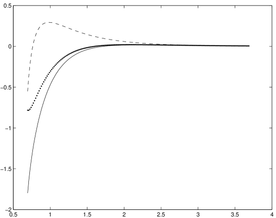
Figure 5: $\mathcal{T}_{t}^{t(0)}$ (solid) , $\mathcal{T}_{r}^{r(0)}$ (dotted), and $\mathcal{T}_{\varphi}^{\varphi(0)}$ (dashed) for $l=1$, $b=0.3$, $q=0.2$, and $N=1$.

Figure 6: $A(r)$ and $B(r)$ touch the horizontal axis, $C(r)$ (dashed), and $D(r)$ (solid).

The Einstein equations (22) are

$$\frac{\Gamma}{2}(C^{\prime\prime}+D^{\prime\prime})-\frac{\Gamma}{r}B^{\prime}-\frac{1}{r}\left(\Gamma+\frac{r^{2}}{l^{2}}-\frac{bl}{4r}\right)(C^{\prime}+D^{\prime})-\frac{\lambda^{2}l^{2}}{r^{4}}A-\frac{3}{l^{2}}B=\mathcal{T}^{t}{}_{t}^{(0)},$$

$$\frac{\Gamma}{2}(A^{\prime\prime}+D^{\prime\prime})-\frac{1}{r}\left(\Gamma-\frac{r^{2}}{l^{2}}+3\frac{bl}{4r}\right)A^{\prime}-\frac{1}{r}\left(\frac{r^{2}}{l^{2}}-\frac{bl}{4r}\right)(B^{\prime}-2D^{\prime})+\frac{\lambda^{2}l^{2}}{r^{4}}A-\frac{3}{l^{2}}B=\mathcal{T}^{\varphi}{}_{\varphi}^{(0)},$$

$$\frac{\Gamma}{2}(A^{\prime\prime}+C^{\prime\prime})+\frac{1}{r}\left(\Gamma-\frac{r^{2}}{l^{2}}+3\frac{bl}{4r}\right)A^{\prime}-\frac{1}{r}\left(\frac{r^{2}}{l^{2}}-\frac{bl}{4r}\right)(B^{\prime}-2C^{\prime})+\frac{\lambda^{2}l^{2}}{r^{4}}A-\frac{3}{l^{2}}B=\mathcal{T}^{z}{}_{z}^{(0)},$$

$$\frac{\Gamma}{r}A^{\prime}+\frac{1}{r}\left(\frac{r^{2}}{l^{2}}-\frac{bl}{4r}\right)(C^{\prime}+D^{\prime})-\frac{\lambda^{2}l^{2}}{r^{4}}A-\frac{3}{l^{2}}B=\mathcal{T}^{r}{}_{r}^{(0)}.$$ (24)

In Fig. 5, the behavior of the energy-momentum tensor components is shown. As is clear from this figure, the components of the energy-momentum tensor rapidly go to zero outside the skin, so the situation is like what happened in the pure AdS spacetime Deh1 . Then solving the coupled differential equations (24) gives the behavior of the functions $A(r)$, $B(r)$, $C(r)$, and $D(r)$ which are displayed in Fig. 6. As one can see $A(r)=B(r)=0$, and $C(r)$ and $D(r)$ are two different constants. Hence by a redefinition of the $z$ coordinate in Eq. (19) the metric can be written as

$$ds^{2}=-\Gamma dt^{2}+\frac{1}{\Gamma}dr^{2}+\beta^{2}r^{2}d\varphi^{2}+\frac{r^{2}}{l^{2}}dz^{2}.$$ (25)

The above metric describes a static charged black string metric with a deficit angle. So, using a physical Lagrangian based model, we have established that the presence of the Higgs field induces a deficit angle in the charged black string metric.

V Conclusion

We considered the Abelian Higgs field in the background of a static charged black string. The numerical solutions for various values of mass and charge parameters and winding number were obtained. We found that for a fixed horizon radius on increasing the winding number the vortex thickness increases. We also showed that the thickness of the vortex is independent of the charge or mass parameter, as long as the horizon radius and winding number remain fixed. We also considered the extremal black string for various winding numbers and found by numerical calculation that the thickness of the vortex is smaller than that of the non-extremal case. These solutions can be interpreted as stable Abelian hair for these black strings.

Also, the effect of a thin vortex on the charged black string has been investigated. This is done by including the self-gravity of the thin vortex in the charged string background to the first order of the gravitational constant. As in the case of pure AdS Deh1 , Schwarzschild-AdS Deh2 , Kerr-AdS, and Reissner-Nordstrom-AdS Ghez2 spacetimes, we showed that the effect of a thin vortex on the static charged black string is to create a deficit angle in the metric.

Other related problems such as a study of the vortex in the charged rotating black string background and the non-Abelian vortex solution in asymptotically AdS spacetimes, remain to be carried out. Work on these problems is in progress.

References

- (1) R. Ruffini and J. A. Wheeler. Phys. Today 24, 30 (1971).
- (2) D. Sudarsky, Class. Quantum Grav. 12, 579 (1995).
- (3) E. Winstanley, Class. Quantum Grav. 16, 1963 (1999).
- (4) A. Achucarro, R. Gregory, and K. Kuijken, Phys. Rev. D 52, 5729 (1995).
- (5) T. Torii, K. Maeda, and M. Narita, Phys. Rev. D 59, 064027 (1999).
- (6) T. Torii, K. Maeda, and M. Narita, Phys. Rev. D 64, 042116 (2001).
- (7) M. H. Dehghani, A. M. Ghezelbash, and R. B. Mann, Nucl. Phys. B625, 389 (2002).
- (8) A. M. Ghezelbash and R. B. Mann, Phys. Lett B 537, 329 (2002).
- (9) A. Chamblin, J. M. A. Ashbourn-Chamblin, R. Emparan, and A. Sornborger, Phys. Rev. D 58, 124014 (1998).
- (10) A. Chamblin, J. M. A. Ashbourn-Chamblin, R. Emparan, and A. Sornborger, Phys. Rev. Lett. 80, 4378 (1998).
- (11) F. Bonjour and R. Gregory, Phys. Rev. Lett. 81, 5034 (1998).
- (12) F. Bonjour, R. Emparan, and R. Gregory, Phys. Rev. D. 59, 84022 (1999).
- (13) M. H. Dehghani, A. M. Ghezelbash, and R. B. Mann, Phys. Rev. D 65, 044010 (2002).
- (14) A. M. Ghezelbash and R. B. Mann, Phys. Rev. D 65, 124022 (2002).
- (15) J. P. S. Lemos and V. T. Zanchin, Phys. Rev. D 54, 3840 (1996).
- (16) M. H. Dehghani, Phys. Rev. D 66, 044006 (2002).
- (17) H. B. Nielsen and P. Olesen, Nucl. Phys. B61, 45 (1973).
- (18) W. H. Press, S. A. Teukolsky, W. T. Vetterling and B. P. Flannery, Numerical Recipes in FORTRAN (Cambridge University Press, Cambridge, England, 1992).