Classical Implications of
the Minimal Length Uncertainty Relation

Abstract

We study the phenomenological implications of the classical limit of the “stringy” commutation relations $[\hat{x}_{i},\hat{p}_{j}]=i\hbar[(1+\beta\hat{p}^{2})\delta_{ij}+\beta^{\prime}\hat{p}_{i}\hat{p}_{j}]$. In particular, we investigate the “deformation” of Kepler’s third law and apply our result to the rotation curves of gas and stars in spiral galaxies.

I Introduction

In this note, we continue our investigation Chang:2001kn ; Benczik:2002tt of the phenomenological implications of “stringy” commutation relations Kempf:1995su which embody the minimal length uncertainty relation $\Delta x\geq(\hbar/2)(\Delta p^{-1}+\beta\,\Delta p)\;$ of perturbative string theory gross . In particular, we study the classical limit of the “deformed” commutation relations

$$\left[\hat{x}_{i},\hat{p}_{j}\right] = i\hbar\left\{(1+\beta\hat{p}^{2})\,\delta_{ij}+\beta^{\prime}\hat{p}_{i}\hat{p}_{j}\right\}\;,$$ (1)

$$\left[\hat{p}_{i},\hat{p}_{j}\right] = 0\;,$$ (2)

$$\left[\hat{x}_{i},\hat{x}_{j}\right] = i\hbar\,\frac{(2\beta-\beta^{\prime})+(2\beta+\beta^{\prime})\beta\hat{p}^{2}}{(1+\beta\hat{p}^{2})}\left(\hat{p}_{i}\hat{x}_{j}-\hat{p}_{j}\hat{x}_{i}\right)\;,$$ (3)

leading to the following “deformed” Poisson brackets,

$$\{x_{i},p_{j}\} = (1+\beta p^{2})\,\delta_{ij}+\beta^{\prime}p_{i}p_{j}\;,$$ (4)

$$\{p_{i},p_{j}\} = 0\;,$$ (5)

$$\{x_{i},x_{j}\} = \frac{(2\beta-\beta^{\prime})+(2\beta+\beta^{\prime})\beta p^{2}}{(1+\beta p^{2})}\left(p_{i}x_{j}-p_{j}x_{i}\right)\;.$$ (6)

The classical Poisson bracket is required to possess the same properties as the quantum mechanical commutator, namely, it must be anti-symmetric, bilinear, and satisfy the Leibniz rules and the Jacobi Identity. These requirements allow us to derive the general form of our Poisson bracket for any functions of the coordinates and momenta as Benczik:2002tt

$$\{F,G\}=\left(\frac{\partial F}{\partial x_{i}}\frac{\partial G}{\partial p_{j}}-\frac{\partial F}{\partial p_{i}}\frac{\partial G}{\partial x_{j}}\right)\{x_{i},p_{j}\}+\frac{\partial F}{\partial x_{i}}\frac{\partial G}{\partial x_{j}}\{x_{i},x_{j}\}\;,$$ (7)

where repeated indices are summed. Thus, the time evolutions of the coordinates and momenta in our “deformed” classical mechanics are governed by

$$\dot{x}_{i} = \{x_{i},H\}\;=\;\phantom{-}\{x_{i},p_{j}\}\,\frac{\partial H}{\partial p_{j}}+\{x_{i},x_{j}\}\,\frac{\partial H}{\partial x_{j}}\;,$$ (8)

$$\dot{p}_{i} = \{p_{i},H\}\;=\;-\{x_{i},p_{j}\}\,\frac{\partial H}{\partial x_{j}}\;.$$ (9)

In Ref. Benczik:2002tt , we analyzed the motion of objects in central force potentials subject to these equations and found that orbits in $r^{2}$ and $1/r$ potentials no longer close on themselves when $\beta$ and/or $\beta^{\prime}$ are non-zero. This allowed us to place a stringent limit on the value of the minimal length from the observed precession of the perihelion of Mercury,

$$\hbar\sqrt{\beta}<2.3\times 10^{-68}\;\mathrm{m}\;,$$ (10)

which was 33 orders of magnitude below the Planck length.

The natural question to ask next is whether there exist other “deformations” of classical mechanics due to $\beta$ and/or $\beta^{\prime}$ that are either 1) observable even for such a small value of $\hbar\sqrt{\beta}$, or 2) lead to an even more stringent limit due to their absence. In the following, we will look at the “deformation” of Kepler’s third law. We will find that while the deformation is not observable on the scale of the solar system, it may be observable at galactic scales. In fact, such an effect may have already been seen in the rotation curves of gas and stars in spiral galaxies.

II Aspects of the Deformed Classical Mechanics

Before we investigate the deformation of Kepler’s third law, it is worthwhile to discuss some peculiarities of this novel classical dynamics.

First, it is obvious that the Poisson bracket $\{x_{i},x_{j}\}$ in Eq. (6) is not invariant under translations since it is proportional to $(\vec{x}\times\vec{p})_{ij}$. For the special case of $\beta^{\prime}=2\beta$, the Poisson bracket $\{x_{i},x_{j}\}$ is zero to order $\mathcal{O}(\beta)$ and we can recover approximate translational invariance Kempf:1995su .

Second, it is not obvious how to extend the fundamental Poisson brackets to multi-particle systems, nor how to define appropriate ‘canonical transformations’ that leave the fundamental Poisson bracket invariant, even in the case of one-particle systems . For instance, consider the motion of 2 bodies of equal mass in 1D. Let us assume that the dynamics will be described by two sets of ‘canonical’ variables, $(x_{1},p_{1})$ and $(x_{2},p_{2})$, which satisfy

$$\{x_{i},p_{j}\} = \left(1+\beta p_{i}^{2}\right)\delta_{ij}\;,$$ (11)

$$\{p_{1},p_{2}\} = \{x_{1},x_{2}\}\;=\;0\;.$$ (12)

Compare this expression to the multi-dimensional case, Eq. (6). The right hand side of the first line is not $(1+\beta p^{2})\,\delta_{ij}$, where $p^{2}=\sum_{i}p_{i}^{2}$, but $(1+\beta p_{i}^{2})\,\delta_{ij}$. This allows us to assume $\{x_{1},x_{2}\}=0$. If we change the variables naively to those of the center of mass frame,

$$\begin{array}[]{ll}x_{\mathrm{cm}}=\frac{\displaystyle x_{1}+x_{2}}{\displaystyle 2}\;,&p_{\mathrm{cm}}=p_{1}+p_{2}\;,\\ x_{\mathrm{rel}}=x_{1}-x_{2}\;,&p_{\mathrm{rel}}=\frac{\displaystyle p_{1}-p_{2}}{\displaystyle 2}\;,\end{array}$$ (13)

then we find that the sets $(x_{\mathrm{cm}},p_{\mathrm{cm}})$ and $(x_{\mathrm{rel}},p_{\mathrm{rel}})$ are no longer ‘canonical’. Of course, in this deformed dynamics momentum is no longer equal to mass$\,\cdot\,$velocity in general, so it is not surprising that the ‘canonical’ momentum of the center of mass, if it exists, is not equal to the sum of momenta of the individual masses.

Third, consider 1D motion with the Hamiltonian given by

$$H=\frac{p^{2}}{2m}+V(x)\;.$$ (14)

We will not consider any deformations of the Hamiltonian itself though it is conceivable that some sort of modification may be required for the consistency of the theory. The equations of motion read

$$\dot{x} = \{x,H\}\;=\;(1+\beta p^{2})\frac{p}{m}\;,$$ (15)

$$\dot{p} = \{p,H\}\;=\;(1+\beta p^{2})\left(-\frac{\partial V}{\partial x}\right)\;.$$ (16)

As mentioned above, the momentum $p$ is no longer equal to $m\dot{x}$. From these equations, we can derive

$$(1+\beta p^{2})(1+3\beta p^{2})F=m\ddot{x}\;,$$ (17)

where

$$F\equiv-\frac{\partial V}{\partial x}\;.$$ (18)

Thus we obtain a deformation of Newton’s second law $F=m\ddot{x}$. Now, notice that if the force $F$ is gravitational and proportional to the mass $m$, the acceleration $\ddot{x}$ is not mass-independent as usual because of the residual $m$-dependence through the momentum $p$. Therefore, in Eq. (17) the equivalence principle is dynamically violated.

It should be noted that the equivalence principle is already known to be violated in the context of perturbative string theory mende . Fundamental strings, due to their extended nature, are subject to tidal forces and do not follow geodesics. However, in contrast to the current discussion where the systems under consideration are of macroscopic dimensions, the violation discussed in Ref. mende was microscopic in nature. Whether this is another example of UV/IR correspondence in string theory remains to be seen.

III Motion in Central Force Potentials

Let us now consider the motion of an object in a general central force potential where the Hamiltonian is given by

$$H=\frac{p^{2}}{2m}+V(r)\;,\qquad r=\sqrt{x_{i}x_{i}}\;.$$ (19)

We will apply the results of this section later to the case when $V(r)$ is the gravitational potential and derive a “deformed” version of Kepler’s third law.

As shown in Ref. Benczik:2002tt , the rotational symmetry of the Hamiltonian Eq. (19) leads to the conservation of the ‘deformed’ angular momentum

$$L_{ij}=\frac{x_{i}p_{j}-x_{j}p_{i}}{(1+\beta p^{2})}\;,$$ (20)

which in turn implies that the motion will be confined to a 2-dimensional plane. Expressing the position of the object in the plane in polar coordinates $(r,\phi)$, the equations of motion can be cast into the form

$$\dot{r} = \frac{1}{m}[\,1+(\beta+\beta^{\prime})p^{2}\,]\,p_{r}\;,$$ (21)

$$\dot{p}_{r} = \frac{1}{mr}[\,1+(\beta+\beta^{\prime})p^{2}\,]\left\{(p^{2}-p_{r}^{2})-\left(mr\frac{\partial V}{\partial r}\right)\left(\frac{1-\beta p^{2}+2\beta p_{r}^{2}}{1+\beta p^{2}}\right)\right\}\;,$$ (22)

$$\dot{\phi} = \frac{L}{mr^{2}}\left\{[\,1+(\beta+\beta^{\prime})p^{2}\,](1+\beta p^{2})+[\,(2\beta-\beta^{\prime})+(2\beta+\beta^{\prime})\beta p^{2}\,]\left(mr\frac{\partial V}{\partial r}\right)\right\}\;,$$ (23)

where

$$p_{r} \equiv \frac{(p\cdot x)}{r}\;=\;\sqrt{p^{2}-\frac{L^{2}(1+\beta p^{2})^{2}}{r^{2}}}\;,$$ (24)

$$L^{2} \equiv -\frac{1}{2}L_{ij}L_{ji}\;=\;\frac{p^{2}\,r^{2}-(p\cdot x)^{2}}{(1+\beta p^{2})^{2}}\;.$$ (25)

We restrict our attention to circular orbits and impose the constraints $\dot{r}=0$ and $\dot{p}_{r}=0$. These conditions lead to

$$L=\frac{p\,r}{(1+\beta p^{2})}\;,$$ (26)

and

$$\left(mr\frac{\partial V}{\partial r}\right)=p^{2}\left(\frac{1+\beta p^{2}}{1-\beta p^{2}}\right)\;.$$ (27)

The radius of the orbit $r$, and the magnitude of the momentum $p=\sqrt{p^{2}}$ are now constants of motion. So is the angular velocity $\omega\equiv\dot{\phi}$ which can be expressed as

$$\omega = \frac{p}{mr}\left\{[\,1+(\beta+\beta^{\prime})p^{2}\,]+\frac{(2\beta-\beta^{\prime})+(2\beta+\beta^{\prime})\beta p^{2}}{(1+\beta p^{2})}\left(mr\frac{\partial V}{\partial r}\right)\right\}$$ (28)

$$= \frac{p}{mr}\left\{[\,1+(\beta+\beta^{\prime})p^{2}\,]+\frac{(2\beta-\beta^{\prime})+(2\beta+\beta^{\prime})\beta p^{2}}{(1-\beta p^{2})}\,p^{2}\right\}$$ (29)

$$= \left(\frac{p}{mr}\right)\frac{(1+\beta p^{2})^{2}}{(1-\beta p^{2})}\;.$$ (30)

Solving Eq. (27) for $p$ and substituting into Eq. (30) yields

$$m^{2}v^{2}=m^{2}r^{2}\omega^{2}=\left(mr\frac{\partial V}{\partial r}\right)f(\varepsilon)\;,$$ (31)

where

$$f(\varepsilon) \equiv \frac{1}{2}\Biggl{[}\,(1+4\varepsilon-\varepsilon^{2})+(1+\varepsilon)\sqrt{1+6\varepsilon+\varepsilon^{2}}\,\Biggr{]}\;,$$ (32)

$$\varepsilon \equiv \beta mr\frac{\partial V}{\partial r}\;.$$ (33)

The function $f(\varepsilon)$ is a monotonically increasing function of $\varepsilon$ which behaves as

$$f(\varepsilon)=\left\{\begin{array}[]{ll}1+4\varepsilon+\mathcal{O}(\varepsilon^{2})&\mbox{when $\varepsilon\ll 1$}\;,\\ 4\varepsilon+\mathcal{O}(\varepsilon^{-1})&\mbox{when $\varepsilon\gg 1$}\;.\end{array}\right.$$ (34)

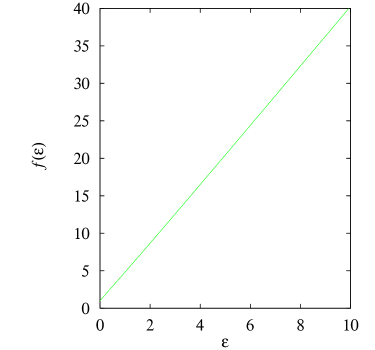
Figure 1: The behavior of the function $f(\varepsilon)$.

The graph of $f(\varepsilon)$ is shown in Fig. 1.

Note that $\beta^{\prime}$ does not appear in our expression for $v^{2}$. This means that the orbital period $T=2\pi r/v$ is not affected by $\beta^{\prime}$. In particular, it is independent of whether approximate translational invariance ($\beta^{\prime}=2\beta$) is realized or not. Note also that $\varepsilon$, and thus the deformation factor $f(\varepsilon)$, depends not only on $r$ but also on $m$. As was the case with Eq. (17), this last fact can be interpreted as the dynamical violation of the equivalence principle when our formalism is applied to motion in gravitational fields.

IV Kepler’s Third Law

For a spherically symmetric mass distribution, the gravitational force on a mass $m$ at a distance $r$ from the center is given by

$$\frac{\partial V}{\partial r}=m\,\frac{GM(r)}{r^{2}}\;,$$ (35)

where $G$ is Newton’s gravitational constant, and $M(r)$ is the total mass enclosed within the radius $r$. Thus, Eq. (31) leads to the relation

$$v^{2}=\frac{GM(r)}{r}\,f(\varepsilon)\;,$$ (36)

with

$$\varepsilon=\beta m^{2}\frac{GM(r)}{r}\;.$$ (37)

In terms of the orbital period $T=2\pi r/v$, we obtain

$$\frac{r^{3}}{T^{2}}=\frac{GM(r)}{4\pi^{2}}\,f(\varepsilon)\;.$$ (38)

This is the ‘deformed’ version of Kepler’s third law.

Planet	mass	eccentricity	semi-major axis	orbital period	apparent	predicted
	$m$ ($10^{24}$kg)	$e$	$a$ ($10^{11}$m)	$T$ ($10^{7}$s)	$\left(\frac{\displaystyle a^{3}}{\displaystyle T^{2}}\frac{\displaystyle 4\pi^{2}}{\displaystyle GM_{\odot}}\right)-1$	$f(\varepsilon)-1$
Venus	$4.869$	$0.00677323$	$1.0820893$	$1.9414149$	$+1\times 10^{-6}$	$6\times 10^{-9}$
Earth	$5.974$	$0.01671022$	$1.4959789$	$3.1558149$	$+3\times 10^{-6}$	$6\times 10^{-9}$
Mars	$0.6419$	$0.09341233$	$2.2793664$	$5.9355036$	$-6\times 10^{-5}\;$	$5\times 10^{-11}$
Jupiter	$1899$	$0.04839266$	$7.7841203$	$37.435566$	$+1\times 10^{-3}$	$1\times 10^{-4}$
Saturn	$568.5$	$0.05415060$	$14.267254$	$92.929236$	$+4\times 10^{-4}$	$6\times 10^{-6}$
Uranus	$86.8$	$0.04716771$	$28.709722$	$265.13700$	$+1\times 10^{-3}$	$7\times 10^{-8}$
Neptune	$102$	$0.00858587$	$44.982529$	$520.04186$	$+1\times 10^{-3}$	$6\times 10^{-8}$

Table 1: The apparent and predicted violation of Kepler’s third law in planetary orbits.

Let us estimate how large this deformation can be for the planets in our solar system. Using the data from Ref. AstroData , we calculate the deformation factor $f(\varepsilon)$ for the planets setting $\beta$ equal to the upper bound provided in Eq. (10). The results are shown in Table 1.

We also list the values of

$$\left(\frac{a^{3}}{T^{2}}\frac{4\pi^{2}}{GM_{\odot}}\right)-1\;,$$ (39)

which show the apparent violation of Kepler’s third law. Note that for elliptical orbits, the radius $r$ must be replaced by the semi-major axis $a$. (We have not included Mercury or Pluto in our list since the eccentricities of these planets are rather large and the circular orbit approximation is poor.)

As can be seen from Table 1, the expected size of the deviation due to our deformed dynamics is orders of magnitude below the apparent deviation which can be explained by classical Newtonian dynamics as a result of perturbations of the planets on each other. Even in the case of Jupiter, for which the predicted deviation is the largest, the deviation due to the deformation is an order of magnitude smaller than the apparent deviation.

Therefore, we can conclude that as long as the constraint given in Eq. (10) is fulfilled, any deformation of Kepler’s third law due to non-zero $\beta$ is completely hidden under apparent violations due to more conventional effects.

V Rotation Curves of Spiral Galaxies

The deformation of Kepler’s third law will affect the $r$-dependence of $v^{2}$. So let us consider whether our deformed dynamics could provide a non-dark matter solution to the halo dark matter problem.

The halo dark matter problem pertains to the rotation curves of interstellar gas in spiral galaxies. ‘Rotation curve’ refers to the plot of $v^{2}$ as a function of the distance $r$ from the galactic center. If gravity due to the visible stars is the only force responsible for the centripetal acceleration, then the observed distribution of stars and Kepler’s third law tell us that $v^{2}$ should fall off asymptotically as $\sim 1/r$ as $r$ is increased. However, the actual observed rotation curves approach constant values instead, suggesting the existence of dark matter halos to account for the missing mass halo1 .

In our deformed dynamics, the correction term $f(\varepsilon)$ does increase the value of $v^{2}$ for a given mass distribution. Unfortunately, the deformation parameter $\varepsilon=\beta m^{2}GM(r)/r$ itself falls off as $\sim 1/r$ with $r$, so the correction vanishes for large $r$ and cannot explain the plateau of the rotation curves. What our formalism does predict, however, is that the size of the correction will be different for different masses due to the $m$-dependence of $\varepsilon$: larger masses will rotate at higher speeds at the same radius $r$, in clear violation of the equivalence principle.

Curiously, it has been recently observed that the rotation curves of stars and interstellar gas do not in general agree when measured separately halo1 ; halo2 . Could our ‘deformed’ dynamics account for this difference? For most galaxies it turns out that the gas rotates at higher speeds than the massive stars. This may have a natural explanation by positing that the gas interacts differently with the dark matter and magnetic fields as compared to the stars. However, for two exceptional galaxies reported in Ref. halo2 , the stars are rotating at much higher speeds than the gas. For the galaxy NGC7331, the speeds of the stars and gas at distance $R_{e}/4$ from the center of the galaxy ($R_{e}$ is the radius which encloses half of the visible light from the galaxy) are reported to be

$$v_{\mathrm{gas}} = \phantom{0}79\pm 20\;\mathrm{km/s}\;,$$ (40)

$$v_{\mathrm{star}} = 186\pm 10\;\mathrm{km/s}\;.$$ (41)

If we interpret this galaxy as a case where the mechanisms that would normally accelerate the gas over the stars are absent and the effect of ‘deformed’ dynamics is manifest, we can ask what value of $\beta$ would account for this difference. Since

$$v^{2} = \frac{GM(r)}{r}\left\{1+4\beta m^{2}\frac{GM(r)}{r}+\cdots\right\}$$ (42)

$$= \frac{GM(r)}{r}\left(1+4\beta m^{2}v^{2}+\cdots\right)\;,$$ (43)

then

$$\frac{v_{\mathrm{star}}^{2}}{v_{\mathrm{gas}}^{2}}\approx 1+4\beta m_{\mathrm{star}}^{2}v_{\mathrm{star}}^{2}\;,$$ (44)

where we have neglected the correction term for the gas. If we assume the solar mass

$$M_{\odot}=2\times 10^{30}\,\mathrm{kg}\;,$$ (45)

as a typical mass of a star in this galaxy, we find

$$\hbar\sqrt{\beta}\sim 10^{-69}\,\mathrm{m}\;,$$ (46)

which is well within the limit given by Eq. (10) and thus compatible with observations on the scale of the solar system.

VI Conclusion and Discussion

In this note, we have investigated possible observable consequences of the “deformed” Kepler’s third law as implied by the classical limit of the “stringy” commutation relations, Eq. (3), which were in turn based on the minimal length uncertainty relation of perturbative string theory gross .

Due to the stringent limit on $\beta$, Eq. (10), obtained from the precession of the perihelion of Mercury in a previous publication Benczik:2002tt , the predicted sizes of the deviations for the planets are too small to be observed. However, the effect of the deformation can be amplified at galactic scales due to the large momenta involved and lead to significant changes in the rotation curves of stars in spiral galaxies.

It would be interesting to contrast our deformed classical mechanics with another modification of Newton’s theory, MOND (Modified Newtonian Dynamics) MOND , which apparently succeeds in predicting a flat rotation curve by modifying Newton’s second law to

$$F\sim m\,\frac{|\ddot{x}|}{a_{0}}\,\ddot{x}\;,$$ (47)

at very small accelerations ($\ddot{x}\ll a_{0}\sim 10^{-10}\,\mathrm{m/s^{2}}$). Our deformed dynamics predicts different rotation curves for different masses, so it is apparently quite different from MOND which does not violate the equivalence principle. Nevertheless, it is interesting to ask whether there exists a deformation of the usual Hamiltonian dynamics which incorporates some kind of UV/IR relation and is in the same universality class as MOND. We hope to address this question in the future.

References

-
(1)
L. N. Chang, D. Minic, N. Okamura, and T. Takeuchi,
Phys. Rev. D 65, 125027 (2002) [hep-th/0111181];
Phys. Rev. D 65, 125028 (2002) [hep-th/0201017]. -
(2)
S. Benczik, L. N. Chang, D. Minic, N. Okamura, S. Rayyan and T. Takeuchi,
Phys. Rev. D 66, 026003 (2002) [hep-th/0204049]. -
(3)
A. Kempf, J. Math. Phys. 35, 4483 (1994) [hep-th/9308025];
A. Kempf, G. Mangano and R. B. Mann, Phys. Rev. D 52, 1108 (1995) [hep-th/9412167];
A. Kempf, J. Phys. A 30, 2093 (1997) [hep-th/9604045]. -
(4)
D. J. Gross and P. F. Mende,
Phys. Lett. B 197, 129 (1987);
D. J. Gross and P. F. Mende, Nucl. Phys. B 303, 407 (1988);
D. J. Gross, Phys. Rev. Lett. 60, 1229 (1988);
D. Amati, M. Ciafaloni and G. Veneziano, Phys. Lett. B 197, 81 (1987);
D. Amati, M. Ciafaloni and G. Veneziano, Int. J. Mod. Phys. A 3, 1615 (1988);
D. Amati, M. Ciafaloni and G. Veneziano, Phys. Lett. B 216, 41 (1989);
K. Konishi, G. Paffuti and P. Provero, Phys. Lett. B 234, 276 (1990);
E. Witten, Phys. Today 49 (4), 24 (1997). -
(5)
P. F. Mende, hep-th/9210001;
R. Lafrance and R. C. Myers, Phys. Rev. D 51, 2584 (1995) [hep-th/9411018];
L. J. Garay, Int. J. Mod. Phys. A 10, 145 (1995) [gr-qc/9403008]. -
(6)
Explanatory Supplement to the Astronomical Almanac,
edited by P. K. Seidelmann (University Science Books, Mill Valley, CA 1992);
Allen’s Astrophysical Quantities, 4th edition, edited by A. N. Cox
(Springer-Verlag, New York 2000);
NASA JPL Solar System Dynamics Group website (http://ssd.jpl.nasa.gov/phys_props_planets.html);
K. Hagiwara et al. [Particle Data Group Collaboration], Phys. Rev. D 66, 010001 (2002). - (7) E. Battaner and E. Florido, Cosmic Phys. 21, 1 (2000) [astro-ph/0010475].
- (8) J. C. Vega Beltán, A. Pizzella, E. M. Corsini, J. G. Funes, S. J., W. W. Zeilinger, J. E. Beckman, and F. Bertola, astro-ph/0105234.
-
(9)
M. Milgrom,
Astrophys. J. 270, 365 (1983);
Astrophys. J. 270, 371 (1983);
Astrophys. J. 270, 384 (1983); astro-ph/0112069;
Scientific American, August 2002 issue, page 42;
R. H. Sanders and S. S. McGaugh, Annual Reviews of Astronomy & Astrophysics, vol. 40 (to be published) [astro-ph/0204521] and references therein.