Deconstructing Scalar QED at Zero and Finite Temperature

Abstract

We calculate the effective potential for the WLPNGB in a world with a circular latticized extra dimension. The mass of the WLPNGB is calculated from the one-loop quantum effect of scalar fields at zero and finite temperature. We show that a series expansion by the modified Bessel functions is useful to calculate the one-loop effective potentials.

I Introduction

It seems obvious that we lives in the four dimensional world. Nevertheless, many theories for unification of forces and/or matter in more dimensions than four have been studiedKK . A simple possibility is that there is a fifth dimension of very tiny size attached to every point of our four-dimensional world. Such an extra dimension can hardly be seen by virtue of its extraordinary smallness.

Last year, there appears a novel scheme to describe higher-dimensional gauge theories, which is called as deconstructionACG ; HPW . A number of copies of a four-dimensional theory linked by a new fields can be viewed as a single gauge theory. The resulting whole theory may be almost equivalent to a higher-dimensional theory with discretized extra dimensions.

Recently, Hill and Leibovich pointed out that the Wilson line pseudo-Nambu-Goldstone boson (WLPNGB) with low mass can be naturally obtained by deconstructing five-dimensional QEDHL1 ; HL2 . This WLPNGB may be a important candidate for a cosmological quintessence.

For cosmological application, we should take finite-temperature effect into account. The behavior of the WLPNGB field may vary along with the cosmological evolution.

In this paper, we examine the $U(1)$ gauge theory with a discretized circle. We obtain the effective potential for the WLPNGB at zero and finite temperature analytically. Through this paper, we consider the one-loop effect of charged scalar bosons. Although this model appears unnatural in contrast to the model with fermionsHL1 ; HL2 , the similar technique is valid for the other models and the application to various models will be studied elsewhere.

In Sec. II, our model is explained and the mass spectra of the component fields are shown. In Sec. III, the one-loop quantum effect of scalar fields is calculated at zero temperature. In Sec. IV, the one-loop quantum effect of scalar fields is calculated at finite temperature. The final section, Sec. V, is devoted to conclusion.

II model

We begin with the lagrangian for deconstructing $(d+1+1)$-D scalar QED:

$${\cal L} = \sum_{k=1}^{N}\frac{1}{g^{2}}\left[-\frac{1}{4}F_{k}^{\mu\nu}F_{k~{}\mu\nu}-(D^{\mu}U_{k})^{\dagger}D_{\mu}U_{k}\right]+\sum_{k=1}^{N}\left[-(D^{\mu}\tilde{\phi}_{k})^{\dagger}D_{\mu}\tilde{\phi}_{k}\right]$$ (1)

$$+ f\sum_{k=1}^{N}\left(\sqrt{2}\tilde{\phi}_{k}^{*}U_{k}\tilde{\phi}_{k+1}+\sqrt{2}\tilde{\phi}_{k}^{*}U_{k-1}^{*}\tilde{\phi}_{k-1}-2f\tilde{\phi}_{k}^{*}\tilde{\phi}_{k}\right)-m^{2}\sum_{k=1}^{N}\tilde{\phi}_{k}^{*}\tilde{\phi}_{k}\,,$$

where

$$F_{k}^{\mu\nu}=\partial^{\mu}\tilde{A}_{k}^{\nu}-\partial^{\nu}\tilde{A}_{k}^{\mu}\,,\qquad D^{\mu}\tilde{\phi}_{k}=\partial^{\mu}\tilde{\phi}_{k}-i\tilde{A}_{k}^{\mu}\tilde{\phi}_{k}\,.$$ (2)

and

$$D^{\mu}U_{k}=\partial^{\mu}U_{k}-i\tilde{A}_{k}^{\mu}U_{k}+iU_{k}\tilde{A}_{k+1}^{\mu}\,.$$ (3)

The label of the fields are considered as periodic modulo $N$, e.g., $\phi_{N+1}\equiv\phi_{1}$, $\phi_{0}\equiv\phi_{N}$, and so on. $N$ is assumed to be larger than $(d+1)/2$. Usually, the dimension of the space is taken as three. We leave the dimensions unfixed because of the possibility in some combination of compactification schemes in the very early universe.

We assume that all $U_{k}$ have a common absolute value $|U_{k}|=f/\sqrt{2}$. Hence we can write

$$U_{k}=\frac{f}{\sqrt{2}}\exp\left(i\tilde{\chi}_{k}/f\right)\,.$$ (4)

It is convenient to use the “Fourier transformed” modes for the fields:

$$\tilde{A}_{k}^{\mu}=\frac{1}{\sqrt{N}}\sum_{p}A_{p}^{\mu}\exp\left[2\pi i\frac{pk}{N}\right]\,,\qquad\tilde{\phi}_{k}=\frac{1}{\sqrt{N}}\sum_{p}\phi_{p}\exp\left[2\pi i\frac{pk}{N}\right]\,,$$ (5)

and

$$\tilde{\chi}_{k}=\frac{1}{\sqrt{N}}\sum_{p}\chi_{p}\exp\left[2\pi i\frac{pk}{N}\right]\,.$$ (6)

The fields $A_{p}^{\mu}~{}(p\neq 0)$ acquire masses by “absorbing” the $\chi_{p}~{}(p\neq 0)$; the mass spectrum is given by

$$4f^{2}\sin^{2}\left(\frac{\pi p}{N}\right)\,.$$ (7)

For small $p$, this mass spectrum is approximately given by

$$f^{2}\left(\frac{2\pi p}{N}\right)^{2}\,,$$ (8)

which is the Kaluza-Klein spectrum in the continuum theory with the circle of the circumference $L=N/f$.

The masses of charged bosons are

$$M_{p}^{2}=4f^{2}\sin^{2}\left(\frac{\pi p}{N}+\frac{\bar{\chi}}{2f}\right)+m^{2}\,,$$ (9)

where $\bar{\chi}\equiv\chi_{0}/\sqrt{N}$ is a (classically) zero-mode scalar field.

III the effective potential at zero temperature

III.1 the one-loop effective potential

In this section, we compute the quantum effect of the scalar fields at zero temperature. The one-loop effective potential for $\bar{\chi}$ is obtained by

$$\ln\det[-\nabla^{2}+M^{2}_{p}(\bar{\chi})]$$ (10)

$$\sim -\frac{1}{(2\pi)^{d+1}}\sum_{p}\int_{0}^{\infty}\frac{dt}{t}~{}\int d^{d+1}{\bf k}~{}\exp\left[-({\bf k}^{2}+M_{p}^{2})t\right]$$

$$= -\frac{1}{(4\pi)^{(d+1)/2}}\int_{0}^{\infty}\frac{dt}{t}t^{-(d+1)/2}~{}\sum_{p}\exp\left[-M_{p}^{2}t\right]\,,$$

after an appropriate regularization.

Using the formula

$$\exp\left[-4f^{2}\sin^{2}(\theta/2)t\right] = e^{-2f^{2}t}\sum_{\ell=-\infty}^{\infty}\cos\ell\theta~{}I_{\ell}(2f^{2}t)$$ (11)

$$= e^{-2f^{2}t}\sum_{\ell=-\infty}^{\infty}e^{i\ell\theta}I_{\ell}(2f^{2}t)\,,$$

where $I_{\nu}(x)$ is the modified Bessel function, we can write the effective potential as

$$V_{0}(\bar{\chi})=-\frac{2}{(4\pi)^{(d+1)/2}}\sum_{p}\sum_{\ell=1}^{\infty}\cos{\ell\theta_{p}}~{}{\cal I}(\ell;m)\,,$$ (12)

where

$$\theta_{p}\equiv\frac{2\pi p}{N}+\frac{\bar{\chi}}{f}\,,$$ (13)

and

$${\cal I}(\ell;m)=\int_{0}^{\infty}\frac{dt}{t^{(d+3)/2}}e^{-(2f^{2}+m^{2})t}I_{\ell}(2f^{2}t)\,.$$ (14)

Here the term which is independent of $\bar{\chi}$ is discarded.

Carrying out the summation over $p$ first, we find that only the term of $p=qN~{}(q:integer)$ is left. Then we find

$$V_{0}(\bar{\chi})=-\frac{2N}{(4\pi)^{(d+1)/2}}\sum_{q=1}^{\infty}\cos(qN\bar{\chi}/f)~{}{\cal I}(qN;m)\,.$$ (15)

III.2 $m=0$

First, we examine the case of $m=0$ in detail. One can findGR

$${\cal I}(qN;0)=(4f^{2})^{\frac{d+1}{2}}\frac{\Gamma(\frac{d+2}{2})\Gamma(qN-\frac{d+1}{2})}{\sqrt{\pi}\Gamma(qN+\frac{d+1}{2}+1)}\,.$$ (16)

Therefore the effective potential for the WLPNGB is written as

$$V_{0}(\bar{\chi})=-\frac{2N\Gamma(\frac{d+2}{2})f^{d+1}}{\pi^{(d+2)/2}}\sum_{q=1}^{\infty}\frac{\Gamma(qN-\frac{d+1}{2})}{\Gamma(qN+\frac{d+1}{2}+1)}\cos(qN\bar{\chi}/f)\,.$$ (17)

In particular, when $d=3$, we obtain

$$V_{0}(\bar{\chi})=-\frac{3f^{4}}{2\pi^{2}}\sum_{q=1}^{\infty}\frac{\cos(qN\bar{\chi}/f)}{q(q^{2}N^{2}-1)(q^{2}N^{2}-4)}\,.$$ (18)

Turning back to the case with general $d$, we find that the effective potential for a large $N$ can be expressed as

$$V_{0}(\bar{\chi})=-\frac{2\Gamma(\frac{d+2}{2})}{\pi^{(d+2)/2}L^{d+1}}\left[\sum_{q=1}^{\infty}\frac{\cos(qL\bar{\chi})}{q^{d+2}}+\frac{(d+1)(d+2)(d+3)}{24N^{2}}\sum_{q=1}^{\infty}\frac{\cos(qL\bar{\chi})}{q^{d+4}}+O(N^{-4})\right]\,,$$ (19)

where $L\equiv N/f$.

The mass of the $\chi_{0}$ field is derived from the effective potential and turns out to be

$$m^{2}_{\chi}=\frac{2\Gamma(\frac{d+2}{2})\tilde{g}^{2}}{\pi^{(d+2)/2}L^{d-1}}Z(d,N)\,,$$ (20)

with

$$Z(d,N)\equiv\sum_{q=1}^{\infty}\frac{q^{2}N^{d+2}\Gamma(qN-\frac{d+1}{2})}{\Gamma(qN+\frac{d+1}{2}+1)}=\zeta(d)+\frac{(d+1)(d+2)(d+3)}{24N^{2}}\zeta(d+2)+O(N^{-4})\,,$$ (21)

where $\zeta(s)$ is the Riemann zeta function and $\tilde{g}=g/\sqrt{N}$. Note that the kinetic term of $\chi_{0}$ includes the factor $\tilde{g}^{-2}$.

$Z(3,N)$ and $Z(2,N)$ are plotted against $N$ in FIG. 1. It is safe to say that the approximation by “Large $N$ Limit” is very good even for $N\approx 10$.

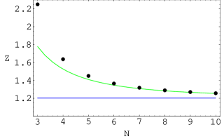
(a)

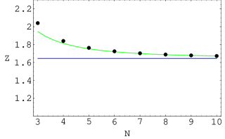
(b)

Figure 1: (a) $Z(3,N)$ is plotted against $N$. The horizontal line indicates $\zeta(3)$. The curve illustrates the approximated value up to the order $N^{-2}$. (b) $Z(2,N)$ is plotted against $N$. The horizontal line indicates $\zeta(2)$. The curve illustrates the approximated value up to the order $N^{-2}$.

III.3 $m\gg f$

For finite $m$, Eq. (14) reduces toGR

$${\cal I}(qN;m) = (2f^{2}+m^{2})^{\frac{d+1}{2}}\left(\frac{f^{2}}{2f^{2}+m^{2}}\right)^{qN}\frac{\Gamma(qN-\frac{d+1}{2})}{\Gamma(qN+1)}$$ (22)

$$\times{}_{2}F_{1}\left(\frac{qN-\frac{d+1}{2}}{2},\frac{qN-\frac{d-1}{2}}{2};qN+1;\frac{4f^{4}}{(2f^{2}+m^{2})^{2}}\right)$$

$$= m^{d+1}\left(\frac{f^{2}}{m^{2}}\right)^{qN}\frac{\Gamma(qN-\frac{d+1}{2})}{\Gamma(qN+1)}{}_{2}F_{1}\left(qN-\frac{d+1}{2},qN+\frac{1}{2};2qN+1;-\frac{4f^{2}}{m^{2}}\right)\,,$$

where ${}_{2}F_{1}$ is the Gauss’ hypergeometric function.

In the large $N$ limit, ${\cal I}(qN;m)$ behaves as $e^{-mqN/f}$ for large $m$. For finite $N$, however, ${\cal I}(qN;m)$ approaches to zero not exponentially but in power law. We find that when $m\gg f$ Eq. (22) reduces to

$${\cal I}(qN;m)\sim m^{d+1}\left(\frac{f^{2}}{m^{2}}\right)^{qN}\frac{\Gamma(qN-\frac{d+1}{2})}{\Gamma(qN+1)}\qquad(m\gg f)\,.$$ (23)

Thus we obtain

$$V_{0}(\bar{\chi})\sim-\frac{2m^{d+1}}{(4\pi)^{(d+1)/2}}\left(\frac{f^{2}}{m^{2}}\right)^{N}\frac{\Gamma(N-\frac{d+1}{2})}{\Gamma(N)}\cos(N\bar{\chi}/f)\qquad(m\gg f)\,.$$ (24)

Correspondingly, the mass of the $\chi_{0}$ field reads

$$m^{2}_{\chi}\sim\frac{2\tilde{g}^{2}m^{d-1}}{(4\pi)^{(d+1)/2}}\left(\frac{f^{2}}{m^{2}}\right)^{N-1}\frac{N^{2}\Gamma(N-\frac{d+1}{2})}{\Gamma(N)}\qquad(m\gg f)\,,$$ (25)

which can be very small value if we choose an appropriate value for $f/m$. This fact suggests that the model can bring about interesting models in cosmological application.

IV the effective potential at finite temperature

IV.1 the finite-temperature effective potential

We know that, to study the finite temperature effective potential, the integration over the frequency is replaced by the summation over the discrete Matsubara frequencies (and attach a certain factor)ft . The free energy density is then obtained by

$$F = -\frac{1}{(2\pi)^{d}\beta}\sum_{p}\sum_{n^{\prime}=-\infty}^{\infty}\int_{0}^{\infty}\frac{dt}{t}~{}\int d^{d}{\bf k}~{}\exp\left\{-\left[\left(\frac{2\pi}{\beta}\right)^{2}{n^{\prime}}^{2}+{\bf k}^{2}+M_{p}^{2}\right]t\right\}$$ (26)

$$= -\frac{1}{(4\pi)^{(d+1)/2}}\int_{0}^{\infty}\frac{dt}{t}t^{-(d+1)/2}~{}\sum_{p}\sum_{n=-\infty}^{\infty}\exp\left[-M_{p}^{2}t-\frac{\beta^{2}n^{2}}{4t}\right]\,,$$

where $T=\beta^{-1}$ is the temperature. Obviously, the $n=0$ term in the summation gives the effective potential at zero temperature.

Now we write $F$ in the form

$$F=V_{0}(\bar{\chi})+\Delta V(\bar{\chi})+F_{0}\,.$$ (27)

Performing the summation over $p$, one can see that the finite-temperature correction to the potential $\Delta V(\bar{\chi})$ results in

$$\Delta V(\bar{\chi})=-\frac{4N}{(4\pi)^{(d+1)/2}}\sum_{q=1}^{\infty}\cos\left[qN\frac{\bar{\chi}}{f}\right]~{}{\cal T}(qN;m)\,,$$ (28)

and

$$F_{0}=-\frac{2N}{(4\pi)^{(d+1)/2}}~{}{\cal T}(0;m)\,,$$ (29)

where

$${\cal T}(\ell;m)=\sum_{n=1}^{\infty}\int_{0}^{\infty}\frac{dt}{t^{(d+3)/2}}~{}\exp\left[-(2f^{2}+m^{2})t-\frac{\beta^{2}n^{2}}{4t}\right]I_{\ell}(2f^{2}t)\,.$$ (30)

Expanding the modified Bessel functions, we can carry out the integration and obtain

$${\cal T}(qN;m)$$ (31)

$$= 2(2f^{2}+m^{2})^{(d+1)/2}(f^{2}/(2f^{2}+m^{2}))^{qN}$$

$$\times \sum_{r=0}^{\infty}\frac{(f^{2}/(2f^{2}+m^{2}))^{2r}}{r!\Gamma(qN+r+1)}\sum_{n=1}^{\infty}\left(\frac{\sqrt{2f^{2}+m^{2}}\beta n}{2}\right)^{2r+qN-\frac{d+1}{2}}K_{2r+qN-\frac{d+1}{2}}(\sqrt{2f^{2}+m^{2}}\beta n)\,,$$

where $K_{\nu}(z)$ is the McDonald function (or the second type of the modified Bessel function).

IV.2 the high-temperature limit

In the high-temperature limit $\beta\rightarrow 0$, the summation over $n$ can be replaced by integration and the following approximation is obtained:

$${\cal T}(qN;m) \sim \frac{\sqrt{\pi}}{\beta}(2f^{2}+m^{2})^{\frac{d}{2}}\left(\frac{f^{2}}{2f^{2}+m^{2}}\right)^{qN}\frac{\Gamma(qN-\frac{d}{2})}{\Gamma(qN+1)}$$ (32)

$$\times{}_{2}F_{1}\left(\frac{qN-\frac{d}{2}}{2},\frac{qN-\frac{d}{2}+1}{2};qN+1;\frac{4f^{4}}{(2f^{2}+m^{2})^{2}}\right)$$

$$= \frac{\sqrt{\pi}}{\beta}m^{d}\left(\frac{f^{2}}{m^{2}}\right)^{qN}\frac{\Gamma(qN-\frac{d}{2})}{\Gamma(qN+1)}{}_{2}F_{1}\left(qN-\frac{d}{2},qN+\frac{1}{2};2qN+1;-\frac{4f^{2}}{m^{2}}\right)$$

$$\qquad(\beta^{-1}\gg f,m)\,.$$

There occurs nothing but the so-called dimensional reduction phenomenon in high-temperature field theory.

In the case of $m=0$, the high-temperature limit leads to

$${\cal T}(qN;0)\sim\frac{1}{\beta}(4f^{2})^{\frac{d}{2}}\frac{\Gamma(\frac{d+1}{2})\Gamma(qN-\frac{d}{2})}{\Gamma(qN+\frac{d}{2}+1)}\qquad(\beta^{-1}\gg f)\,,$$ (33)

and the effective potential becomes

$$V(\bar{\chi})\equiv V_{0}(\bar{\chi})+\Delta V(\bar{\chi})\sim-\frac{2N\Gamma(\frac{d+1}{2})f^{d}}{\beta\pi^{(d+1)/2}}\sum_{q=1}^{\infty}\frac{\Gamma(qN-\frac{d}{2})}{\Gamma(qN+\frac{d}{2}+1)}\cos(qN\bar{\chi}/f)\quad(\beta^{-1}\gg f)\,.$$ (34)

Particularly, for $d=3$,

$$V(\bar{\chi})\sim-\frac{2f^{3}}{\beta\pi^{2}}\sum_{q=1}^{\infty}\frac{N\cos(qN\bar{\chi}/f)}{(q^{2}N^{2}-1/4)(q^{2}N^{2}-9/4)}\qquad(\beta^{-1}\gg f)\,,$$ (35)

is obtained. For general $d$ and large $N$, we find

$$V(\bar{\chi}) \sim -\frac{2\Gamma(\frac{d+1}{2})}{\beta\pi^{(d+1)/2}L^{d}}\left[\sum_{q=1}^{\infty}\frac{\cos(qL\bar{\chi})}{q^{d+1}}+\frac{d(d+1)(d+2)}{24N^{2}}\sum_{q=1}^{\infty}\frac{\cos(qL\bar{\chi})}{q^{d+3}}+O(N^{-4})\right]$$ (36)

$$\qquad(\beta^{-1}\gg f)\,,$$

where $L\equiv N/f$.

The mass of the $\chi_{0}$ field in the high-temperature limit is

$$m^{2}_{\chi}\sim\frac{2\Gamma(\frac{d+1}{2})\tilde{g}^{2}}{\beta\pi^{(d+1)/2}L^{d-2}}Z(d-1,N)\qquad(\beta^{-1}\gg f)\,,$$ (37)

where $Z(d,N)$ has been defined as Eq. (21).

In the case that $\beta^{-1}\gg m\gg f$, we find

$${\cal T}(qN;m) \sim \frac{\sqrt{\pi}}{\beta}m^{d}\left(\frac{f^{2}}{m^{2}}\right)^{qN}\frac{\Gamma(qN-\frac{d}{2})}{\Gamma(qN+1)}\qquad(\beta^{-1}\gg m\gg f)\,,$$ (38)

and this leads to

$$V(\bar{\chi})\sim-\frac{2m^{d}}{\beta(4\pi)^{d/2}}\left(\frac{f^{2}}{m^{2}}\right)^{N}\frac{\Gamma(N-\frac{d}{2})}{\Gamma(N)}\cos(N\bar{\chi}/f)\qquad(\beta^{-1}\gg m\gg f)\,.$$ (39)

The mass of the $\chi_{0}$ field is then

$$m^{2}_{\chi}\sim\frac{2\tilde{g}^{2}m^{d-2}}{\beta(4\pi)^{d/2}}\left(\frac{f^{2}}{m^{2}}\right)^{N-1}\frac{N^{2}\Gamma(N-\frac{d}{2})}{\Gamma(N)}\qquad(\beta^{-1}\gg m\gg f)\,.$$ (40)

The mass-square of the $\chi_{0}$ increases with temperature linearly.

IV.3 temperature dependence of the free energy

In the rest of this section, we investigate the leading temperature dependence of the free energy. Though the contribution of the gauge fields is of course present, we concentrate ourselves only on the contribution of the scalar fields.

The dominant dependence on temperature can be found in $F_{0}$. Let us remember

$${\cal T}(0;m)=2(2f^{2}+m^{2})^{(d+1)/2}$$

$$\qquad\times\sum_{r=0}^{\infty}\frac{(f^{2}/(2f^{2}+m^{2}))^{2r}}{r!\Gamma(r+1)}\sum_{n=1}^{\infty}\left(\frac{\sqrt{2f^{2}+m^{2}}\beta n}{2}\right)^{2r-\frac{d+1}{2}}K_{2r-\frac{d+1}{2}}(\sqrt{2f^{2}+m^{2}}\beta n)\,,$$ (41)

where we should notice $K_{\nu}(z)=K_{-\nu}(z)$.

At extremely high temperature ($\beta^{-1}\gg f,m$), the $r=0$ term is dominant and using the limiting form for a small argument $K_{\nu}(z)\sim\frac{1}{2}\Gamma(|\nu|)(z/2)^{-|\nu|}$, one obtains

$${\cal T}(0;m)\sim\frac{2^{d+1}\Gamma(\frac{d+1}{2})\zeta(d+1)}{\beta^{d+1}}\qquad(\beta^{-1}\gg f,m)\,.$$ (42)

Then this leads to

$$F\sim F_{0}\sim-\frac{2N\Gamma(\frac{d+1}{2})\zeta(d+1)}{\pi^{(d+1)/2}\beta^{d+1}}\qquad(\beta^{-1}\gg f,m)\,.$$ (43)

This is precisely the free energy for $N$ (effectively) massless charged bosons. This behavior can be derived from the original form of ${\cal T}(0;m)$

$${\cal T}(0;m) = \sum_{n=1}^{\infty}\int_{0}^{\infty}\frac{dt}{t^{(d+3)/2}}~{}\exp\left[-(2f^{2}+m^{2})t-\frac{\beta^{2}n^{2}}{4t}\right]I_{0}(2f^{2}t)$$ (44)

$$= \frac{1}{\beta^{d+1}}\sum_{n=1}^{\infty}\frac{1}{n^{d+1}}\int_{0}^{\infty}\frac{dt}{t^{(d+3)/2}}~{}\exp\left[-(2f^{2}+m^{2})\beta^{2}n^{2}t-\frac{1}{4t}\right]I_{0}(2f^{2}\beta^{2}n^{2}t)\,,$$

with the limiting form $I_{0}(z)\sim 1$ for a small argument.

On the other hand, for $\beta^{-1}\ll f$, Eq. (44) can be approximated, using $I_{0}(z)\sim e^{z}/\sqrt{2\pi z}$ for a large argument, as

$${\cal T}(0;m)\sim\frac{2}{\sqrt{4\pi}~{}f\beta^{d+2}}\sum_{n=1}^{\infty}\left(\frac{2\beta m}{n}\right)^{\frac{d+2}{2}}K_{\frac{d+2}{2}}(\beta mn)\qquad(\beta^{-1}\ll f)\,.$$ (45)

This leads to

$$F\sim F_{0}\sim-\frac{4N}{(4\pi)^{(d+2)/2}~{}f\beta^{d+2}}\sum_{n=1}^{\infty}\left(\frac{2\beta m}{n}\right)^{\frac{d+2}{2}}K_{\frac{d+2}{2}}(\beta mn)\qquad(\beta^{-1}\ll f)\,.$$ (46)

Further, if we assume $m\ll\beta^{-1}$, it is found that

$${\cal T}(0;m)\sim\frac{2^{d+2}\Gamma(\frac{d+2}{2})\zeta(d+2)}{\sqrt{4\pi}~{}f\beta^{d+2}}\qquad(m\ll\beta^{-1}\ll f)\,.$$ (47)

Then in this case,

$$F\sim F_{0}\sim-\frac{2\Gamma(\frac{d+2}{2})\zeta(d+2)}{\pi^{(d+2)/2}\beta^{d+2}}\frac{N}{f}\qquad(m\ll\beta^{-1}\ll f)\,,$$ (48)

is obtained. This result coincides with the one of the finite-temperature continuum Kaluza-Klein theory with circle length $L=N/f$RR , after replacing the scalar degree of freedom.

We have found that $(-F)$ behaves as $T^{d+1}$ at high temperature, while it behaves as $T^{d+2}$ at lower temperature than $f$. This fact indicates that the dimension of the spacetime seems $d+2$ for $T<f$ and again $d+1$ for $T>f$. Of course, at very low temperature $T\ll f/N$, as one can see from Eq. (26) for $m=0$ and $\bar{\chi}=0$,

$$F\sim-\frac{2\Gamma(\frac{d+1}{2})\zeta(d+1)}{\pi^{(d+1)/2}\beta^{d+1}}\qquad(\beta^{-1}\ll f/N)\,.$$ (49)

So, we recognize the world as $(d+1)$-dimensional spacetime with the lowest-mode field at very low temperature.

V conclusion

In conclusion, the effective potential for the WLPNGB in scalar QED with a discretized dimension has been calculated at zero and finite temperature. We have utilized the expansion in terms of the modified Bessel functions, which is also useful for computing the one-loop effect in models with more discretized (or, latticized) dimensionsfw . We have found that approximating the one-loop effect by large $N$ expansion is valid if the model has a limiting form of infinite $N$.

We have also found that the $(mass)^{2}$ of the WLPNGB increases linearly with high temperature. This serves some possibilities: Coherent oscillations of the WLPNGB field may change the frequency according to the expansion of the universe, or, if domain walls might be produced, their mass density decreases as temperature decreases. Furthermore, novel temperature-dependence of energy density may bring interesting consequences to the very early universe. These cosmological implications will be clarified after analyzing more realistic models and incorporating other matter fields.

We should consider the one-loop effect of fermions for more natural particle theory. Moreover degenerate fermions may largely affect the WLPNGB mass and the entire potential. These subjects will be discussed elsewheremi .

References

(1) T. Appelquist, A. Chodos and P. G. O. Freund,
Modern Kaluza-Klein Theories, Addison-Wesley, 1987.
(2) N. Arkani-Hamed, A. G. Cohen and H. Georgi,
Phys. Rev. Lett. 86 (2001) 4757;
Phys. Lett. B513 (2001) 232.
(3) C. T. Hill, S. Pokorski and J. Wang,
Phys. Rev. D64 (2001) 105005.
(4) C. T. Hill and A. K. Leibovich,
Phys. Rev. D66 (2002) 016006,
hep-ph/0205057.
(5) C. T. Hill and A. K. Leibovich,
“Natural Theories of Ultra-Low Mass PNGB’s: Axions and Quitessence”,
hep-ph/0205237.
(6) I. S. Gradstein and I. M. Ryshik,
Tables of integrals, sums, series and products,
Academic Press, New York (1980).
(7) J. I. Kapusta,
Finite-temperature field theory, CUP, 1989;
M. Le Bellac,
Thermal Field Theory, CUP, 1996.
(8) M. A. Rubin and B. D. B. Roth,
Nucl. Phys. B226 (1982) 444.
(9) K. Shiraishi, K. Sakamoto and N. Kan,
“Shape of Deconstruction”, hep-ph/0209126.