SU(2) gauged Skyrme-monopoles in scalar-tensor gravity
Abstract
Considering a Skyrme model with a peculiar gauging of the symmetry, monopole-like solutions exist through a topological lower bound. However, it was recently shown that these objects cannot form bound states in the limit of vanishing Skyrme coupling. Here we consider these monopoles in scalar-tensor gravity. A numerical study of the equations reveals that neither the coupling to gravity nor to the scalar dilaton nor to dilaton-gravity leads to bound multimonopole states.
I Introduction
A few years ago topologically stable solutions with nonvanishing magnetic flux were constructed [1] in a particular SU(2) gauged SU(2) SU(2) sigma model. This model differs essentially from the (gauged) Skyrme model [2] because in place of the usual pion–mass potential of the latter, it is characterised by a potential which leads to the breaking of the SU(2) symmetry down to U(1), resulting in a monopole charge. The gauging prescription is given by Eq. (6) of [1] and we employ the constrained non-linear sigma field , with () instead of . The diagonal part of the SU(2) SU(2) global symmetry is gauged by means of the standard introduction of appropriate Yang-Mills fields (see [1] Eqs. (7)-(8) for details).
The construction of the spherically symmetric solution () and of the axially symmetric solutions [3] in the limit of vanishing Skyrme coupling indicates that the mass per winding number of the solution exceeds that of the solution by roughly three percent, leading to the conclusion that classical bound states are not possible.
On the other hand, in the much more popular bosonic part of the SU(2) Georgi-Glashow model which allows for monopole solutions with [4, 5], it is well known that in the Prasad-Sommerfield limit of vanishing Higgs mass [6] monopoles are non-interacting [7] and thus the mass of the monopole of topological charge is exactly times the mass of the single monopole solution. Recently, it was demonstrated that coupling of the Georgi-Glashow model to gravity [8] and/or to a scalar field (the “dilaton”) [9, 10, 11] results in bound multimonopole solutions.
It thus seems sensible to couple the gauged non-linear sigma model of [1] to gravity and/or a dilaton and to analyze if this new attracting interaction can lead to bound states.
The numerical results we have obtained reveal that neither the coupling to gravity nor to the dilaton nor to dilaton-gravity can render an attractive phase in the model studied here. We describe the model in Section II. In Section III and IV, we describe the spherically symmetric, respectively axially symmetric Ansatz and the obtained numerical results. We give our conclusions in Section V.
II The model
The model is described by the Lagrangian of the field , and an SU(2) valued gauge field :
| (1) |
with covariant derivative
| (2) |
and field strength tensor
| (3) |
In the following we work in the temporal gauge (thus the solutions carry only a magnetic charge) and assume . We are here premarily interested in the effect of scalar-tensor gravity in the case of vanishing . The reason for this is that for , the results in [3] suggest that the monopoles are already in an attractive phase in flat space and thus the coupling to gravity would increase this attraction. We are here more interested to see whether gravity and/or a dilaton can overcome the repulsion of flat space (similar as it can in the case of non-vanishing Higgs self-coupling in the Georgi-Glashow model [8]).
The coupling of the matter field to a (massless) dilaton field consists in replacing above by means of
| (4) |
where the coupling constant to the dilaton is denoted by .
The coupling to gravity is done by adding the Einstein-Hilbert action :
| (5) |
where is defined above while
| (6) |
with denoting Newton’s constant. Note that the dilaton can be decoupled by setting .
III Spherically symmetric solutions
The spherically symmetric Ansatz for the field is described by
| (7) |
| (8) |
for the matter fields,
| (9) |
for the metric and for the dilaton field.
We use the following rescaling :
| (10) |
The classical equations which are obtained after an algebra then depend only on the dimensionless coupling constants and :
| (11) |
| (12) |
| (13) |
| (14) |
| (15) |
These equations are solved subject to the following boundary conditions for the gravitating (resp. dilatonic) case :
| (16) |
| (17) |
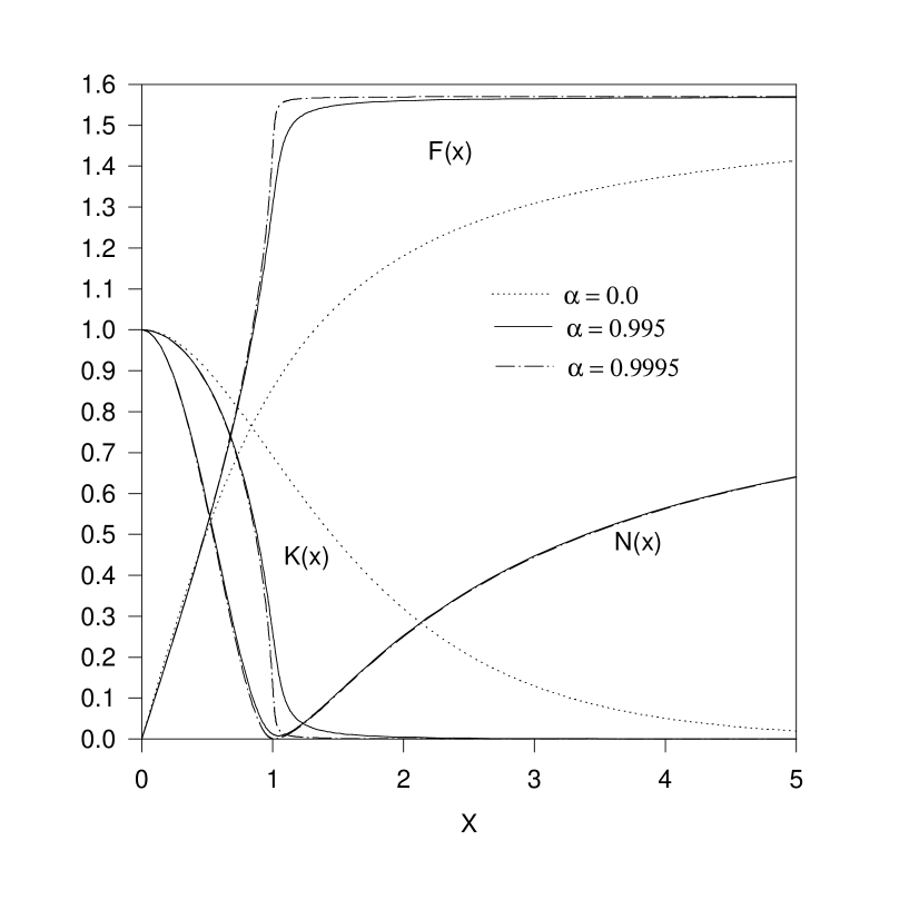
Note that for , the equations admit a topological soliton with classical mass in units . The corresponding profiles of and are presented in Fig. 1.
If we set , we recover the equations for the gauge field function and dilaton function (13), (15) of the SU(2) Einstein-Yang-Mills-Higgs-dilaton (EYMHD) model [12] in the BPS limit. The Einstein equations and the equation for the scalar field function, however, are modified. Denoting by the rhs of the corresponding EYMHD equations (see [12]) arising in the Georgi-Glashow model, we rewrite (11), (12), (14) in terms of :
| (18) |
and
| (19) |
with the abbreviations
| (20) |
| (21) |
We first solved the equations in the gravitating case () for generic values of . The gauged skyrmion solution of [1] is slightly deformed in a way very reminiscent to the gravitating monopole [13] : the function develops a local minimum which becomes deeper with increasing . For a maximal value of this minimum is equal to zero at , the matter fields and vary mainly on and reach their asymptotic value for . On the interval the solution approaches an extremal Reissner-Nordström solution [13]. Our numerical analysis strongly suggests that , . This maximal value is approached directly, i.e. there is no backbending as in the gravitating GG-model for small value of the Higgs boson mass.
The value can be compared to those obtained in the Georgi-Glashow (GG) model for gravitating monopoles. It lies between the value of vanishing Higgs boson mass (BPS limit) and that of the infinite Higgs mass limit . We have not succeeded in finding an analytic explanation for this phenomenon. In our case the equation for the -field remains non trivial while the corresponding equation is just trivially fulfilled in the limit of infinite Higgs mass [13] in the GG model and reproduces a power expansion of the solutions which is more predictive.
The fact that the maximal value of (i.e. ) is much larger than in the GG-monopole case with infinite Higgs mass () might be understood by comparing the masses in both models for the flat case. Defining as the ratio of the Higgs boson mass and the vector boson mass in the GG-model, it is well known [14] that the monopole mass (in units of , being the vacuum expectation value of the Higgs field) is such that
| (22) |
We note that in flat space the mass of our gauged Skyrme-monopole is very close to the mass of the GG-monopole for . On the other hand, it was shown [15] that for the gravitating GG-monopoles. Since the mass density is the main parameter determining the formation of a limiting black hole solution, this provides a consistent argument that should be of the order of unity for the gravitating gauged Skyrme-monopole.
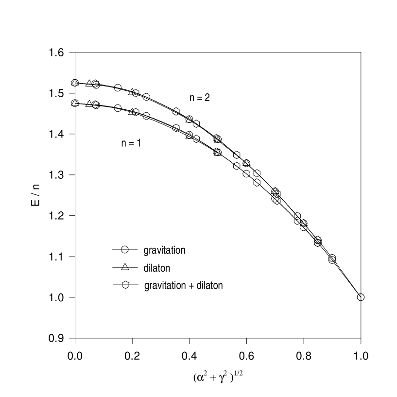
The profiles of the functions at the approach of the critical value are shown in Fig. 1 together with the flat space profiles. The mass of the gravitating solution as a function of is plotted in Fig. 2 (, circles).
We then solved the equations in the purely dilatonic case (, ) which implies . We found a similar pattern as in the Georgi-Glashow model coupled to a dilaton [16] : the flat solution is gradually deformed by the dilaton field, the value is negative and decreases while increases and becomes infinite in the limit . Our numerical analysis strongly suggest that . The mass of the dilatonic solution is shown in Fig. 2 as function of (, triangles). It hardly differs from its counterpart for gravitating solutions as function of . The similarities between the influence of a gravitating field and of a dilatonic field on solitons was noticed previously in [16] and in [9] for SU(2) Yang-Mills-Higgs theories. Our results demonstrate that this analogy persists for Skyrme-like solutions. It is furthermore easy to see that the correspondence between the -component of the metric and the dilaton found previously for the GG-monopoles [12] is also valid here.
More remarkably, solving the equations for fixed leads to identical curves for the mass ) (within the numerical inaccuracy) irrespective of of the choice of and . Thus plotting the mass as function of leads to a curve very similar to the pure gravitating and pure dilatonic one. This is demonstrated in Fig. 2 (, hexagons). In the limit of critical coupling, the solutions for , bifurcate with the Einstein-Maxwell-dilaton (EMD) solutions, very similar to the solutions in SU(2) Einstein-Yang-Mills-Higgs-dilaton (EYMHD) theory [12].
IV Axially symmetric solutions
The axially symmetric Ansatz for the metric in isotropic coordinates reads:
| (23) |
The functions , and now depend on and . If and only depend on , this metric reduces to the spherically symmetric metric in isotropic coordinates and comparison with the metric in (9) yields the coordinate transformation [17]:
| (24) |
For the gauge fields we choose the purely magnetic Ansatz:
| (25) |
| (26) |
while for the sigma-field, the Ansatz reads [3]
| (27) |
The vectors , and are given by:
| (28) | |||||
| (29) | |||||
| (30) |
The dilaton field now depends on and [9]:
| (31) |
At the origin, the boundary conditions read:
| (32) |
| (33) |
At infinity, the requirement for finite energy and asymptotically flat solutions leads to the boundary conditions:
| (34) |
| (35) |
In addition, boundary conditions on the symmetry axes (the - and -axes) have to be fulfilled. On both axes:
| (36) |
and
| (37) |
After a similar rescaling as in (10) we have solved the classical equations numerically for . The energy per winding number of the solutions is presented in Fig. 2 for the dilatonic (triangles), gravitating (circles) and dilatonic-gravitating (hexagons) case as function of . Like for , the similarity of the dependence of the masses on the parameter is striking.
The other main point of this figure is that we find for all three cases. Although the difference is maximal in the flat case ( and/or ) (it is about three percent of the mass of the classical lump) it decreases, as expected, for and/or . However, neither the gravitating nor the dilatonic nor the dilatonic-gravitating interaction is strong enough to overcome the repulsion.
Let us finally remark, that our numerical results strongly suggest (although with less accurancy than in the spherically symmetric case ) that the solution for bifurcates into an extremal Reissner-Nordström black hole at exactly . The plot of the quantity as a function of clearly shows that it tends to zero in the limit and that at the same time the angle dependence of vanishes. Since the extremal Reissner-Nordström solution in isotropic coordinates has a horizon located at , the pattern described above is a signature of a bifurcation into an extremal RN black hole [8, 17]. Similarly, the corresponding extremal solutions in isotropic coordinates are reached in the limit of critical coupling in the pure dilatonic, respectively dilatonic-gravitating case.
V Concluding remarks
The gauged skyrmion model proposed in [1] and the corresponding topological solutions constitute an alternative to the celebrated Georgi-Glashow model and its (multi-)monopoles. It supports a magnetic charge and, because of a topological inequality, exists even in absence of a Skyrme term ().
In this paper, we were mainly interested in the questions whether bound states of gauged Skyrme-monopoles are possible. In the absence of a Skyrme term, bound states are not possible in flat space [3]. A natural step then was to study whether gravitating or dilatonic (or both) interactions can lead to an attractive phase (similarly as in the Georgi-Glashow model for small enough Higgs boson mass). Unfortunately, we found that this is not possible and likely, the construction of bound states of gauged Skyrme-monopoles will require a non-vanishing Skyrme term (for which in flat space there already seems to be an attraction).
However, we believe that the results presented here reveal a potentially interesting property of the model: it seems that the limit corresponds to a bifurcation of the and solutions into a Reissner-Nordström black hole with magnetic charge and mass (in suitable units). Attempts to explain the occurence of the value algebraically are under investigation.
Acknowledgements: We gratefully acknowledge discussions with D. H. Tchrakian. B. H. was supported by the EPSRC.
REFERENCES
- [1] Y. Brihaye, B. Hartmann and D. H. Tchrakian, J. Math. Phys. 42 (2001), 3270.
- [2] T.H.R. Skyrme, Nucl. Phys., Proc. Roy. Soc. A 260 (1961), 127; Nucl. Phys. 31 (1962) 556.
- [3] Y. Brihaye, B. Hartmann and D. H. Tchrakian, J. Math. Phys. 43 (2002), in press.
- [4] G. ’t Hooft, Nucl. Phys. B79 (1974), 276; A. M. Polyakov, JETP Lett. 20 (1974), 194.
- [5] C. Rebbi and P. Rossi, Phys. Rev. D22 (1980), 2010; P. Forgacs, Z. Horvard and L. Palla, Phys. Lett. 99B (1981), 232; M. K. Prasad and P. Rossi, Phys. Rev. D24 (1981), 2182; R. S. Ward, Commun. Math. Phys. 79 (1981), 232; E. Corrigan and P. Goddard, Commun. Math. Phys. 80 (1981), 575.
- [6] M. K. Prasad and C. M. Sommerfield, Phys. Rev. Lett. 35 (1975), 159; E. B. Bogomol’nyi, Sov. J. Nucl. Phys. 24 (1976), 449.
- [7] N.S. Manton, Nucl. Phys. B 126 (1977), 525; W. Nahm, Phys. Lett. 79B (1978), 426; Phys. Lett. 85B (1979), 373; J. N. Goldberg, P. S. Jang, S. Y. Park and K. C. Wali, Phys. Rev. D16 (1978), 542; L. O’ Raifeartaigh, S. Y. Park and K. C. Wali, Phys. Rev. D20 (1979), 1941;
- [8] B. Hartmann, B. Kleihaus and J. Kunz, Phys. Rev. Lett. 86 (2001) 1422.
- [9] Y. Brihaye and B. Hartmann, Phys. Lett. B528 (2002), 288.
- [10] Y. Brihaye and B. Hartmann, Phys. Lett. B534 (2002), 137.
- [11] B. Hartmann, Phys. Lett. B541 (2002), 369.
- [12] Y. Brihaye, B. Hartmann and J. Kunz, Phys. Rev. D65 (2002), 024019.
- [13] P. Breitenlohner, P. Forgacs and D. Maison, Nucl. Phys. B383 (1992), 357.
- [14] E. B. Bogomol’nyi and M. S. Marinov, Yad. Fiz. 23 (1976), 676.
- [15] P. Breitenlohner, P. Forgacs and D. Maison, Nucl. Phys. B442 (1995), 126.
- [16] P. Forgacs and J. Gyueruesi, Phys. Lett. B366 (1996), 205.
- [17] B. Hartmann, B. Kleihaus and J. Kunz, Phys. Rev. D65 (2002) 024027.