Astrophysics in relative units as the theory of a conformal brane
Abstract
The latest astrophysical data on the Supernova luminosity-distance – redshift relations, primordial nucleosynthesis, value of Cosmic Microwave Background-temperature, and baryon asymmetry are considered as an evidence of relative measurement standard, field nature of time, and conformal symmetry of the physical world. We show how these principles of description of the universe help modern quantum field theory to explain the creation of the universe, time, and matter from the physical vacuum as a state with the lowest energy.
1 Introduction
Observations and measurements of the physical parameters of cosmic objects and their theoretical interpretation within the framework of modern physical theories of space, time, and matter (general relativity [1] and Standard Model of elementary particles [2]) enable one to describe the history of cosmic evolution of the universe in the whole [3].
In particular, observational data on the dependence of the redshifts of spectral lines of atoms on cosmic objects from their distance up to the Earth [4], and the new data [5, 6] for large values of redshifts testify to that our universe is mainly filled with not a massive “dust” of far and, therefore, invisible Galaxies, but with mysterious substance of a much different nature, with a different equation of state called Quintessence [7]. The data including primordial nucleosynthesis and the chemical evolution of the matter in the universe (described in the nice book by Weinberg [8]) point to a definite equation of state of the matter in the universe. This equation helps us to determine a kind of matter taking part in the cosmic evolution of the redshift. The data on the visible number of particles (baryons, photons, neutrinos, etc.) testify to that the visible baryon matter gives only part of the critical density of the observational cosmic evolution [9]. The data on the Cosmic Microwave Background radiation with the temperature and its fluctuations [10] give information about the evolution of the early universe.
Beginning with the pioneer papers by Friedmann [1] and ending with the last papers on inflationary model [2] of the Hot Universe Scenario [11], all observational data are interpreted in the theoretical cosmology as some evidence of the expanding universe. Here, it is necessary to clearly distinguish the expansion of theoretical intervals from the expansion of “measurable intervals” obtained by matching with a particular measurement standard.
Not all clearly understand that this treatment of the Friedmann interval as a measurable one is true, if there are “absolute” units that do not expand together with the cosmic scale factor in the universe, because an observer can measure only a ratio of any physical quantities and the units. Such a conjecture about the absolute measurement standard, irrespective of how it will be selected (as one of the 40.000.000th part of Parisian Meridian or as a definite number of wave lengths of a spectral line of an isotope of krypton–86 [12]), contradicts the Einstein cosmological principle, according to which “any of the averaged characteristics of space environment does not select preferential position or preferential directions in the space” [13].
The real situation is even more complicated. Not all clearly realize that modern cosmology in fact utillizes the dual standard in describing the phenomenon of cosmic evolution of photons emitted by a massive matter on a far cosmic object.
As soon as the cosmic photon has been carved out from atom, there are two distance scales: the wave length of a photon and the size of an atom that is determined by its mass. The observer can measure only evolution of a dimensionless ratio of the size of the atom, emitting a photon on a far cosmic object, to the wave length of this photon. These measurements irrefutably testify only to a permanent magnification of this dimensionless ratio. However, these measurements cannot tell us what exactly is augmented: the wave length of a photon, or the mass of an atom emitting this photon. Thus, the observer who selected the absolute measurement standard of length states that the wave length is augmented; and who selected the relative one, that the mass is augmented.
The relative units are used in observational cosmology to determine initial data for cosmic photons flying to an observer [14], whereas the absolute units are utilized for interpretation of observational data in theoretical cosmology.
Theoretical cosmology considers the description in the relative units only as a mathematical method of solving problems, underlining that there are two mathematically equivalent versions of the theoretical description of cosmological data in the form of two mathematically equivalent versions of general relativity and Standard Model. By virtue of this equivalence the usage of the dual standard in cosmology does not lead to conflicts and enables one to reformulate the theory by treating the relative quantities as measurable ones, and the absolute ones as a mathematical tool of solving problems. As a result we can recalculate all astrophysical data in the relative units, including the conformal time, coordinate distance, and constant temperature , so that the z-history of temperature becomes the z-history of masses.
The attempt of this recalculation made in [14, 15, 16, 17, 18, 19, 20] has shown, that the symmetry of equations of motion of the theory in the relative units increases, and number of phenomenological parameters decreases. This choice of the relative units results in a number of coincidences of parameters of cosmic evolution and elementary particle physics which could be considered as random ones if such coincidences were not so large.
The purpose of the present paper is the description of the results and consequences of the relative measurement standards which expand together with the universe.
2 Astrophysical data in the relative units
Theoretical cosmology is based on general relativity and the Standard Model of elementary particles constructed similarly to the Faraday - Maxwell electrodynamics.
Maxwell revealed that the description of results of experimental measurement of electromagnetic phenomena by the field theory equations depend on the definition of measurable quantities in the theory and the choice of their measurement standard. In the introduction to his A Treatise on Electricity and Magnetism [21] Maxwell wrote: “The most important aspect of any phenomenon from mathematical point of view is that of a measurable quantity. I shall therefore consider electrical phenomena chiefly with a view to their measurement, describing the methods of measurement, and defining the standards on which they depend”.
Defining a measurable interval of the length as the ratio
| (1) |
one need to point out its measurement standard. In modern physics such a measurement standard of length is the Parisian meter equal to a particular number of lengths of a light wave of a concrete spectral line of the krypton isotope - 86 [12].
Physical cosmology based on the expanding interval [1]
| (2) |
with the scale factor uses two standards: the relative and absolute.
Observational conformal cosmology (CC) uses the relative Parisian meter
| (3) |
for measurements of all lengths with the corresponding conformal interval of the space-time
| (4) |
of the cosmic photons flying on the light cone to an observer. This interval is given in terms of the conformal time and coordinate distance.
While in the theoretical standard cosmology (SC) one proposes that all lengths in the universe are measured with respect to the absolute Parisian meter
| (5) |
In the standard cosmology the cosmic factor scales all distances besides the Parisian meter (5). Nobody can explain why the measurement standard is so distinguished in the expanding universe.
Using the light cone equation one can find the coordinate distance - conformal time relation
| (6) |
where is the present-day value of the conformal time when a value of the scale factor is equal to unit . Therefore, the current cosmological time of a photon emitted by an atom at the coordinate distance is equal to the difference
| (7) |
Observational data testifies that the energy of cosmic photons depends on the coordinate distance (6). The energy of the cosmic photons (emitted at the conformal time ) is always less then the similar energy of the Earth photons (emitted at the conformal time ):
| (8) |
where
| (9) |
is the redshift of the spectral lines of atoms at objects at the coordinate distance in comparison with the the present-day spectral lines of atoms at the Earth.
In terms of the relative units (3) and the conformal interval (4) we reveal that the measurable spatial volume of the universe is a constant , while all masses including the Planck mass are scaled by the cosmic scale factor
| (10) |
In this case, we get the relation (8) as an eigenvalue of solutions of the Schrödinger equation with the running mass (10)
| (11) |
It is easy to check that in the limit of eigenvalue of the solution of this equation is expressed throw the one of solution of a similar Schrödinger equation with constant masses at
| (12) |
where is the spectrum of a Coulomb atom111The spectrum of photons emitted by atoms from distant stars billion years ago remains unchanged during the propagation and is determined by the mass of the constituents at the moment of emission. When this spectrum is compared with the spectrum of similar atoms on the Earth which, at the present time, have larger masses, then a redshift is obtained..
It was shown [15, 14, 17] that the relative units give a completely different physical picture of the evolution of the universe than the absolute units of the standard cosmology. The temperature history of the expanding universe copied in the relative units looks like the history of evolution of masses of elementary particles in the cold universe with a constant temperature of the cosmic microwave background.
In the standard cosmology, an absolute measured distance is defined as the product of the scale factor and the coordinate distance . This product can be treated as a conformal transformation that leads to the theory with constant mass.
When we assert that the cosmic factor was equal to the square root of “time” in the epoch of the primordial nucleosynthesis, the question appears: what time does an observer measure by his watch, and what time is identified with the time of chemical evolution?
If this time is absolute, the square root of “time” means that the universe in the epoch of chemical evolution was completed by radiation when density of pressure is equal to one third of the energy density.
If this time is conformal, the square root of “time”
| (13) |
means that the universe in the epoch of chemical evolution was completed by Quintessence when density of pressure is equal to the energy density.
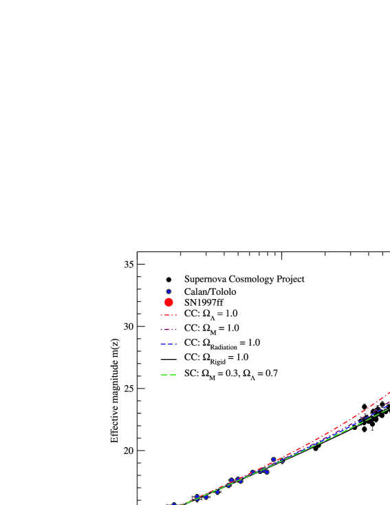
If we identify time of the evolution with conformal time and substitute the law of nucleosynthesis (13) into the Hubble diagram of dependence of redshift on distances to Supernovae, we can reveal [14] that this law corresponds to the black line in a Fig. 1 that is in agreement with all data on the Supernova luminocity–distance — redshift relation [5, 6].
As it was shown in [14], in the case of the relative Parisian meter (3), both the epoch of chemical evolution and the recent experimental data for distant supernovae [5, 6] are described by the square root dependence of the cosmic factor on “time”. This evolution results from the dynamics of a homogeneous scalar field which we call the scalar Quintessence (SQ). This massless field with purely kinetic contribution to the energy density in the universe leads to a rigid equation of state (where pressure is equal to energy) and gives a satisfactory description of the supernova data.
Other consequence of the relative standard of measurement is the redshift independence of the cosmic microwave background temperature [17, 18]. This is at the first glance in a striking contradiction with the observation [22] of . However, the relative population of different energy levels from which the temperature has been inferred in this experiment follows basically the Boltzmann statistics with the same z-dependence of the Boltzmann factors for both the absolute standards and relative one [14]. Therefore, the experimental finding can equally well be interpreted as a measurement of the z-dependence of energy levels (masses) at constant temperature.
Thus, one more argument in favor of the relative units is the sharp simplification of the scenario of the evolution of the universe. Astrophysical data in the relative units can be described by a single epoch with the dominance of Quintessence, while the same data in the absolute units require the scenario with three different epoches (inflation, radiation, and inflation with the dark matter).
3 Conformal symmetry of the world
Any physical theory beginning with Newton at the highest level consists of two parts: I) differential equations of motion and II) the initial data which Laplace still required for unambiguous solutions of the Newton equations and which are measured by a set of physical instruments identified with a frame of reference.
The equations of motion are considered as a kingdom of laws of nature; and the initial data, as a kingdom of freedom. In accelerator high-energy physics the experimenters set the geometry of instruments and initial states of an investigated physical object. The initial data of the universe are probably set by Lord-God, but the essence of theoretical statement of the task remains the same, and, practically does not differ from a school task (14) about a train moving in the one-dimensional space with the coordinate with constant speed from St.-Petersburg to Moscow .
To find the time dependence of the coordinate of the train
| (14) |
it is necessary to solve the Newton equation. This equation does not depend on the initial data (i.e., on the kingdom of freedom of passengers of this train who chose St.-Petersburg as the initial position and the speed of the train ), but the final result of the solution of this task - Moscow - is a consequence of both the kingdoms: the will of the passengers and the laws of Nature. It is important that the Newton equations do not depend on the initial data of the variable .
Independence of the laws of nature on the initial data is called the symmetry of the theory with respect to transformations changing the frame of reference, i.e., rearranging the initial position and speed.
Historically, frame symmetries appeared as the Galilean group of transformations rearranging positions and velocities of the initial data of particles in the Newton mechanics. The frame symmetry of the modern unified theory is the Poincare group of transformations rearranging the initial data of relativistic fields. The Poincare group was recovered by Lorentz and Poincare from the Maxwell equations. All field theories of the 20th century were constructed by analogy with the Maxwell electrodynamics [23]. In particular, the field nature of light in electrodynamics and its relativistic symmetry were an example for Einstein to formulate his gravitation theory. However, an analogy with the Maxwell electrodynamics was incomplete.
The collection of Faraday’s experimental results in the form of Maxwell’s equations testifies to that these equations are invariant with respect to conformal transformations222The conformal group was discovered by Möbius in the 19th century [24], and it was extracted from electrodynamics by Bateman and Cuningham in 1909 [25]. The conformal transformations keep invariant the angle between two vectors in space-time and include the scale transformations..
If to trust that symmetry of the theory of the universe coincides with symmetry of the theory of light, GR and SM in absolute and relative units arise as result of the certain choice of gauge in the conformal–invariant theory of scalar field called dilaton,
| (15) |
where the GR action is replaced by the Penrose—Chernikov—Tagirov action [26] for the scalar field called dilaton
| (16) |
and the Higgs mass in the SM action is replaced by this dilaton . In such a theory all masses are scaled by dilaton . Set of fields including scalar field and SM fields is given in the space with an interval
| (17) |
where are relativistic covariant differential forms with the Fock tetrads .
Action (15) is invariant with respect to the scale transformations:
| (18) | |||||
| (19) | |||||
| (20) |
The Quintessence is treated as the angle of mixing of two scalar fields and given in the dilaton two-dimensional space with the signature (). Two dilatons and four Higgs field before the spontaneous symmetry breaking describe a four-dimensional relativistic brane in six-dimensional external space with the metrics:
The action of this brane
| (21) |
belongs to the class of actions of a relativistic string
| (22) |
where and a relativistic particles
| (23) |
There is the unified method of description of energetics of all three relativistic theories [27, 28]. This method is based on the fact that groups of transformations of all relativistic actions (15), (21), (22), and (23) include reparametrizations of the coordinate evolution parameter
This means that is not observable and the role of measurable evolution parameter is played by one of the dynamic variables. Its canonical momentum plays the role of energy of a relativistic system.
4 The energy of relativistic systems
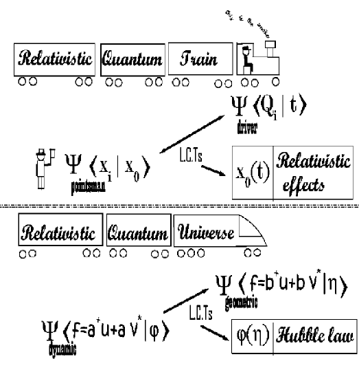
In contrast to the classical mechanics, in the relativistic mechanics, for a complete description of a relativistic particle one needs two observers. In Fig. 2 they are depicted in the role of a pointsman and a driver. A pointsman meters by his watch the time as a variable in the world Minkowskian space of all events, and a driver meters by his watch the time as a geometrical interval on a world line of events. Only both sets of measurements restore a pathway of a particle in the world space as a solution of equations of motion in special relativity (23):
where the momenta of a particle are linked by the mass-shell equation
| (24) |
Here the momentum
| (25) |
is treated as an energy of a particle. Its initial coordinate is treated as the point of its creation or annihilation in the wave function of a particle
| (26) |
where the coefficients are treated as operators of creation, if a particle goes forward, and of annihilation, if a particle goes backward. This causal quantization excludes the negative value of the energy to make stable a quantum state of a particle [27, 28].
The set of measurable quantities and the wave function of a relativistic particle for a driver can be obtained by a transformation of the time as the variable into the time as the geometrical interval [30, 29]. Such transformation was firstly proposed in the theory of differential equations by Levi-Civita as back as 1906 [31]. From the point of view of Newtonian physics, the complete description of any relativistic object is possible by two realizations of this object. For a particle one of such realizations is Minkowskian space, where the evolution parameter is the dynamic variable , and the second is the geometrical realization where the evolution parameter is the time interval . The relationship between these realizations is treated as a new, in principle, element of the scientific explanation of the pure relativistic effects.
The similar choice of the evolution parameter for a relativistic string
| (27) |
was firstly considered by Barbashov and Chernikov [32]. This gauge removes excitations of string with negative norm. It was proved [29] that the string theory in this gauge coincides with the Born—Infeld theory that strongly differs from the Virasoro algebra [33]. Reiman and Faddeev [34] reproduced and generalized this result in 1975. In the paper [29] the energetics of a relativistic string was considered on the basis of the definition of the energy as the canonical momentum of the evolution parameter
| (28) |
The description of the universe with the finite volume and lifetime in the conformal theory (15) is carried out in a frame of reference defined by embedding of three-dimensional hypersurface into the four-dimensional Riemannian space-time
| (29) |
for an observer at rest333An observer moving in the direction of the axis 1 has: .
Following Barbashov and Chernikov (27) we can choose an evolution parameter as homogeneous dilaton with the constant volume
| (30) |
This gauge excludes all modes of the dilaton with a negative norm except of the homogeneous one that becomes the evolution parameter.
In the case of the relative units the conformal invariant action (15) takes the form
| (31) |
The theory (15) with the field evolution parameter gives a physical explanation of a problem of horizon by simultaneous variations of masses of all particles in the whole three-dimensional hypersurface, as a consequence of the symmetry of the theory with respect to reparametrizations of the coordinate parameter in the ADM metrics [35].
The theory (31) has the unambiguous and clear definition of the localizable Hamiltonian of the evolution as the canonical momentum of the field evolution parameter like (25) and (28)
| (32) |
where the Lagrangian is given by the action (31) and is an invariant time interval for the averaged lapse function [18, 30, 29].
In the theory (31), homogeneity of the universe is explained by an average of a precise equation over the volume, instead of “inflation”. In particular, in the theory (31) the equation of evolution of the universe
| (33) |
where , appears as an average of precise equation of the lapse function
| (34) |
over the spatial volume. The solution (33) is an analogy of the Friedmann relationship in the precise theory between the time interval and the cosmic scale factor.
The equation (33) in terms of canonical momentum (32) takes the form of the global energy constraint of the type of the mass-shell equation (24)
| (35) |
where is the contribution of local field excitations and is the one of global homogeneous excitations. In particular, if the homogeneous scalar Quintessence dominates, neglecting all remaining fields, we shall receive a homogeneous action
which in fact is similar to the action of a relativistic particle (23).
Cosmology is defined as such homogeneous approximation of GR of the type of (4) that inherits its symmetry with respect to reparametrization of the coordinate evolution parameter . Reparametrization-invariant cosmological models were firstly considered by DeWitt, Wheeler, and Misner [36, 37], do not differ from the special relativity. There is a direct correspondence between the Minkowskian space-time and the field space of the variables of the model (4) with equations
| (37) |
and their solutions
with the dilaton as the evolution parameter. Quantum theory, in particular, the Wheeler-DeWitt equation
| (38) |
appears as a direct analogy of the Klein-Gordon equation in relativistic quantum field theory. The solution of the Wheeler-DeWitt equation
| (39) |
and its interpretation do not differ from a similar solution of the Klein-Gordon equation for a quantum relativistic particle. To remove negative energies and to construct a stable quantum system in relativistic quantum theory the causal quantizing of fields is postulated. According to this quantizing, the wave with positive energy goes forward; and negative energy, backward. The same treatment of the coefficient as operator of creation of the universe, and , as operator of annihilation of the universe, solves the problem of the cosmic singularity, as a wave function of the universe with positive energy does not contain a point of singularity; the singularity is contained in a wave function with negative energy which is treated as a probability amplitude of annihilation of anti-universe.
Thus, the conformal unified theory (31) in the concrete frame of reference with cosmic initial data gives the possible solutions of the problems of modern cosmology. At least, these solutions should be considered on equal footing with the old scheme conserving Newtonian absolute such as the absolute Parisian meter, or the absolute Planck mass when we fix the gauge of the constant dilaton with the running volume
| (40) |
This gauge appears from (30) by transformation that converts the variable with the initial cosmic data , into its present-day value . This transformation creates in equations of motion the absolute parameter of the Planck mass and the problem of Planck era. The theory in the gauge (40) loses solutions of problems of cosmic initial data, horizon, time and energy, homogeneity, singularity, and quantum wave function of the universe discussed before. These problems are solved by the inflationary model [2].
5 “Creation” of the universe and time
The mathematical structure of general relativity and Standard Model in the relative units (with the evolution parameter and an energy of the universe defined as a value of the canonical momentum of this evolution parameter) allow us to use the analogy with the relativistic particle (26) to construct a wave function of the relativistic universe in the world field space for positive and negative energy with the initial data .
This wave function of the universe
| (41) |
describes the greatest events – the creation of the universe with positive energy flying forward in the field space: the cosmic singularity is in wave function the universe with negative energy flying backward to the point of the singularity.
To make this creation of the universe stable, one constructs the wave function of the quantum universe in the field realization excluding the negative value of the energy from the wave function. To do so, we need to treat the creation of the universe with negative energy as annihilation of the anti-universe with positive energy. This construction is known in quantum field theory as causal quantization with the operators of creation and annihilation of the universe [27, 28]. Consequences of the causal quantization (41) are the positive arrow of the geometric time and its beginning [29, 30] .
The wave function of the universe in the geometric realization
| (42) |
describes the quantum evolution of the universe in the geometric world space with the zero initial data for matter fields.
The universe as a relativistic object can also be completely described by two realizations: field and geometric. Each of them has its world space of variables (field , or geometric ), its evolution parameter (the cosmic scale factor or geometric time ), its initial data, and its wave function (the field , or geometric ).
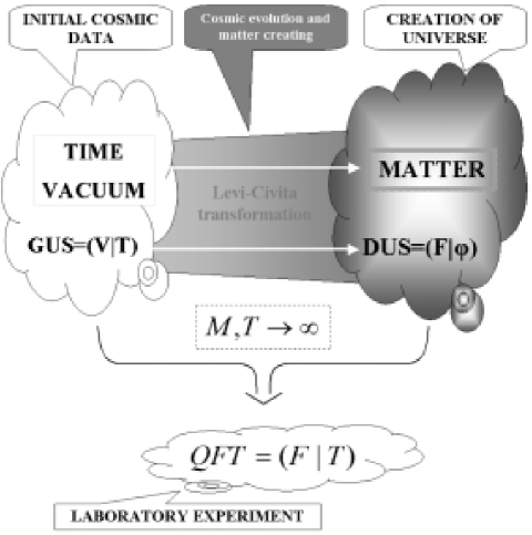
Both these realizations are connected by the Levi-Civita transformations that convert the field space with the field evolution parameter into the geometric world space with the time evolution parameter [30, 29]. The geometrization as a rigorous mathematical construction of the geometric time includes the transformations of the initial fields with a set of quantum numbers into the geometric fields known as the Bogoliubov transformations [38, 39].
The vacuum initial data including a number of particles can be treated as field coordinates of the creation of the universe in its field realization. Such a creation takes place out of time that belongs to another realization of the universe in the geometric space (, ).
The evolution of the cosmic scale factor with respect to time is considered as a pure relativistic effect that is beyond the scope of the Newton-like mechanics.
At the beginning of universe there were only two global excitations in the form of “superfluid motions” (according to the therminology by Landau [40] and Bogoluibov [38]): the running Planck mass and Quintessence. The momenta of these motions are linked as the momenta of a relativistic particle (24). All further evolution of the running Planck mass and measurable number of particles in the field space is treated as the Levi-Civita geometrization of fields in the unified theory [30, 29]. These transformations for local particles coincide with the Bogoliubov transformations in his microscopic theory of superfluid helium [38]: . In our theory these transformations describe cosmological creation of a substance from vacuum in the early universe. The number of created particles is defined as the sum of quadrates of the Bogoliubov coefficients : where the magnitude is called the distribution function of the numbers of particles.
6 Creation of matter
The origin of particles is an open question as the isotropic evolution of the universe cannot create massless particles [39, 41].
Here we list arguments in favor of that the cosmological particle creation from vacuum [41] in the conformal–invariant unified theory can describe the cosmic energy density budget of observational cosmology.
At the first moment of the lifetime of the universe, the frame-fixing quantization [42] of W–, Z– vector bosons in the Standard Model shows us an effect of their intensive cosmological creation [41] from the geometric Bogoliubov vacuum [14, 17, 18]. The distribution functions of the longitudinal and transverse vector bosons calculated in [14, 17, 18] for the initial data are introduced in Fig. 4.
We can speak about the cosmological creation of a pair of massive particles in the universe, when the particle mass is larger than the initial Hubble parameter .
The distribution functions of the longitudinal vector bosons introduced in Fig. 2 show the large contribution of relativistic momenta. This means the relativistic dependence of the particle density on the temperature in the form . These distribution functions show also that the time of establishment of the density and temperature is the order of the inverse primordial Hubble parameter. In this case, one can estimate the temperature from the equation in the kinetic theory [43] for the time of establishment of the temperature
where is the cross-section.
This kinetic equation and values of the initial data help us to calculate the temperature of relativistic bosons [15, 14, 17, 18]
as a conserved number of cosmic evolution compatible with the Supernova data [5, 6] and the primordial chemical evolution [8]. We can see that this calculation gives the value surprisingly close to the observed temperature of the CMB radiation .


A ratio of the density of the created matter to the density of the primordial cosmological motion of the universe has an extremely small number
| (43) |
On the other hand, it is possible to estimate the lifetime of the created bosons in the early universe in dimensionless units , where , by utillizing the equation of state and define the lifetime of –bosons in the Standard Model
| (44) |
where is the Weinberg angle, . The solution of equation (45) gives the value for
| (45) |
The transverse bosons during their lifetime form the baryon symmetry of the universe as a consequence of the “polarization” of the Dirac sea vacuum of left fermions by these bosons, according to the selection rules of the Standard Model [44] with left current interaction in SM for each left doublet marked by an index . At a quantum level, we have an abnormal current
| (46) |
where in the lowest order of perturbation theory . The integration of this equation (46) gives the number of left fermions created during the lifetime of vector bosons [17, 18]
where is the density of number of the CMB photons. The baryon asymmetry appears as a consequence of three Sakharov conditions: -nonconservation, evolution of the universe and the violation of the baryon number [18] where is a factor determined by a superweak interaction of and -quarks with the CP-violation experimentally observed in decays of mesons with a constant of a weak coupling [45].
After the decay of bosons, their temperature is inherited by the Cosmic Microwave Background radiation. All the subsequent evolution of matter with varying masses in the constant Universe replicates the well-known scenario of the hot universe [8], as this evolution is determined by the conformal-invariant ratios of masses and temperature . As the baryon density increases as a mass and the Quintessence density decreases as an inverse square mass, the present-day value of the baryon density can be estimated by the relation
| (47) |
if the baryon asymmetry with the density was frozen by the superweak interaction. This estimation gives the value surprisingly close to the observational density in agreement with the observational data. In the current literature [46] the cosmological creation of particles is considered as an origin of the primordial fluctuations of temperature of CMB [10]. Generally speaking, all these present and future results can only be treated as a set of arguments in favor of the considered unified theory.
Thus, we have shown that the conformal-invariant version of general relativity and Standard Model with geometrization of constraint and frame-fixing with the primordial initial data , (determined by a free homogeneous motion of the Scalar Quintessence, i.e., its electric tension) can describe the following events:
The key differences of such a description from the inflationary model [2] are the absence of the Planck era and cosmological creation of matter from the physical vacuum as a stable state with lowest energy at the moment when the size of the horizon of events in the universe coincides with the Compton length of the vector W-,Z-bosons.
7 Conclusion
The relative measurement standard opens out the well-known truth that the universe is an ordinary physical object with a finite volume and finite lifetime444 It demonstrates us the dark sky at night, to what Halley, de Chéseaux, and Olbers paid attention [47]..
Results of theoretical description of the finite universe depend on the choice of a frame of reference and initial data like the results of solution of the Newton equations depend on initial positions and initial velocities of a particle. Creation of the universe has taken place in a particular frame of reference which was remembered by the cosmic microwave radiation. We remind that the “frame of reference” is identified with a set of the physical instruments for measuring the initial data needed for unambiguous solving differential equations of theoretical physics. These differential equations are invariant structural relations of the whole manifold of all measurable quantities with respect to their transformations. The determination of a group of these transformations is the most important problem of the modern theoretical physics.
There are two types of the transformation groups of differential equations of the gauge theory: frame-transformations that change initial data, i.e., the frame of reference; and gauge-transformations that do not change initial data and are associated with the calibration of physical instruments.
Derivation of frame-covariant and gauge-invariant solutions of differential equations as well as the construction of frame-covariant and gauge-invariant quantization of gauge fields were considered as the mainstream of development of theoretical physics beginning with the work by Dirac [48] and ending with the work by Schwinger in the sixties who called this quantization fundamental [49]. The strategy of this fundamental quantization was to construct gauge-invariant variables in a definite frame of reference and to prove the relativistic invariance of a complete set of results [49, 50, 51].
The basic method of quantization in gauge field theories, however, became the other heuristic quantization, proposed by Feynman [52, 53]. Feynman noticed that the scattering amplitudes of the elementary particles in perturbation theory do not depend on the frame of reference and the gauge choice [52]. The independence of the frame of reference was called simply the relativistic invariance, and the gauge choice became the formal procedure of choosing the gauge non-invariant field variables. It may seem that this slight substitution of the meaning of the concepts in the method heuristic quantization completely depreciates the goals and tasks of the fundamental quantization. Why should we prove the “relativistic invariance“ of a complete set of results at the level of the algebra of the Poincare group generators for gauge-invariant observables, if the result of calculating of each scattering amplitude is relativistic invariant, i.e. does not depend on a frame of reference [54]? What do we need gauge-invariant observables for, if one can use any variables also for solving the problems of construction of the unitary perturbation theory and proving the renormalizability of the Standard Model [55]? The statement and solution of these important problems carried out within the limits of heuristic quantization resulted in that the latter became one and the only method of solving all the problems of the modern field theory. The highest achievements of the abstract formulation are the frame-free quantization of string theories and M-theory as a candidate for the role of a future consistent theory of all interactions with the Planck absolute mass (see, e.g., [56]).
At the end of the past century, a dramatic situation arose in physics, when a historical path of physics - the path of the frame of references, seems to be absolutely interrupted. Remained only the “kingdom of laws” burdened with absolutes independent from a frame of reference. The “kingdom of freedom” of initial data turned out to be enclosed by heuristic quantizing and its claims for a successful solution of all problems. There was a new terminology with the distorted definition of relativistic invariance, suitable only for the description of the tasks of scattering.
However, physicists have forgotten that the simplified heuristic quantizing is proved only for amplitudes of scattering of elementary particles [57], and its applicability is restricted to only scattering problems – the domain where it first appeared [52]. The fundamental quantization is more suitable for the physics of bound states, hadronization and confinement, and for the description of the quantum universe [30, 51]. Yet in 1962, Schwinger [49] pointed out that the frame-free formulations can distort the initial gauge theory and lead to a wrong spectrum of nonlocal collective excitations. Schwinger rejected all frame-free formulations of relativistic theories “as unsuited to the role of providing the fundamental operator quantization” [49]555 Frame-free formulations lead to another spectrum of the nonlocal bound states: when we replace in QED the Dirac sources in the Coulomb gauge of by the Lorentz ones, to acquire the independence on any frame of reference and initial data, we substitute the perturbation theory of fundamental quantization with the two singularities of photon propagators: at the equal time instants and on the light cone, by the perturbation theory in the Lorentz gauge with only one singularity of photon propagators. The latter kind of singularities cannot, in principle, describe the Coulomb atoms at the equal time instants; these singularities describe only the Wick-Cutkosky bound states [58] with the bound state spectrum which are impossible to be observed in the nature..
In 1974, Barbashov and Chernikov [32] applied the frame-fixing formulation to the relativistic string theory and proved that this theory coincided with the Born-Infeld theory that strongly differs from the abstract frame-free formulation of a string with the so-called Virasoro algebra [33]. Reiman and Faddeev [34] reproduced and generalized this result in 1975 (for details see [29]).
The relative measurement standard reverts us on a historical path of physics, the path of frame of references. This path began with relativity by Copernicus, Galilei, and Newton, and it was prolonged by Einstein’s relativity theories and papers by Dirac, Heisenberg, Pauli, Fermi and Schwinger on gauge-invariant fundamental quantizing. It is the path of definition of a transformation group of all measurable physical quantities, which leaves invariant their structural relations called the differential equations. It is the path where all absolutes of theories become, eventually, ordinary initial data.
The relative units reveal that a symmetry group of the whole manifold of measurable physical quantities in the world includes conformal symmetry of the Faraday-Maxwell electrodynamics, and the field nature of matter should also be supplemented by the field nature of space and time.
The relative units lead us to the “kingdom of freedom” of initial data including also last dimensional absolute of modern quantum field theory and those initial data of creation of the universe, for which an observer does not carry any responsibility, as he at this moment existed only as an intention. Who has carried out this experiment of creation of the universe? Who has determined the initial data of this creation? Whose notebook is the wave function of the universe?
Acknowledgment
Authors are grateful to Profs. B.M. Barbashov, D. Blaschke, N.A. Chernikov, P. Flin, J. Lukierski, M.V. Sazhin, and A.A. Starobinsky for fruitful discussions. This work was supported in part by the Bogoliubov-Infeld Programme.
Appendix Appendix A: Penrose–Chernikov–Tagirov
theory in
the Barbashov–Chernikov gauge
We consider the dilaton part of the “brane” (15) described by the PCT action (16) with negative sign
| (A.1) |
The absolute gauge means the choice of the variables by the scale transformation
| (A.2) |
that leads to Einstein‘s general relativity
| (A.3) |
This gauge introduces the absolute parameter into equations of motion together with absolute Planck era.
The Hamiltonian approach to general relativity is well known [36, 37]
| (A.4) |
where
| (A.5) |
is the standard Hamiltonian with the constraints, gauges, and the Lagrangian multipliers , , , discussed in [36, 37, 60].
The Barbashov–Chernikov gauge [32, 34, 29] means the choice of the relative variables by the scale trasformation
| (A.6) |
that keeps the evolution parameter as a dynamic variable in correspondence with the invariance of the theory under reparametrizations of the coordinate evolution parameter.
PCT theory in the terms of relative variables takes the form
| (A.7) |
where the first term coincides with the Einstein action with the Hamiltonian GR:11
| (A.8) |
in terms of relative fields and dynamic evolution parameter instead of the Planck mass ; the second term
| (A.9) |
is interference between the global motion of the universe and the local field excitations; the third term
| (A.10) |
is the action of the global motion of the universe in the field world space, and are considered as functionals given by
| (A.11) |
The interference of the global and local variables disappears, if we impose the Dirac condition [59] of the minimal embedding of the three-dimensional hypersurface into the four-dimensional space-time in the relative space . The minimal embedding removes not only the interference of the global motion with local excitations, but also all local excitations with the negative norm [60].
The PCT theory in terms of relative variables is the direct field generalization of SR with two time–like variables (the geometric interval and dynamic evolution parameter ) and two wave functions. We have one to one correspondence between SR and PCT theory [39, 30], i.e., their proper times
| (A.12) |
their world spaces
| (A.13) |
their energies
| (A.14) |
and their two-time relations in the differential form
| (A.15) |
and in the integral forms
| (A.16) |
Recall that in SR eq. (A.16) can be treated as the Lorentz transformation of the rest frame with time into the comoving one with the proper time . Similarly, in GR the relation defined by eq. (A.16) is treated as a canonical transformation [30]. This correspondence (A.12)-(A.16) allows us to solve the problem of time and energy in GR like Poincare and Einstein [61, 62] had solved it in SR. They identified the time with one of variables in the world space. The similar String/SR correspondence was considered in papers [63, 29].
Appendix Appendix B: The cosmic energetics of Galaxies
In this Appendix the solution of the Kepler problem is given in the Friedman–Robertson–Walker metric [64]. Here we show that the cosmic evolution depresses an energy of particles, urging free particles to be captured in bound states, and free galaxies, in clusters of galaxies.
The formulation of the Kepler problem in the Friedmann—Robertson—Walker (FRW) metrics
| (B.1) |
proposes a choice of physical variables, coordinates, and units of measurement. In particular, the choice of absolute units of the expanding universe means that the coordinates are measurable. In terms of these coordinates the interval (B.1) becomes
| (B.2) |
where is the Hubble parameter, and are the Hubble velocities that should be taken into account in the energy of matter in the universe. The Hubble velocities are contained in the covariant derivatives in the Newton action in the space with the interval (B.2)
| (B.3) |
where is a constant of a Newtonian interaction of a galaxy with a mass in a gravitational field of mass of a cluster of galaxies .
The last three summands in this action (B.3) are identified with the Hamiltonian of a “particle”, a value of which on solutions of equations of motion is called an energy of the system. It is easy to see that the Hubble velocities in action (B.3) are contained in the additional summand in the total energy of the system (B.3)
| (B.4) |
as contrasted to a customary Newtonian energy of the system
for the circular velocity , initial radius , and orbital momentum in the cylindrical coordinates
| (B.5) |
These components of Hubble’s velocity are not taken into account in papers [65, 66, 67, 68] analysing the problem of Dark Matter on the basis of the Newtonian motion of a particle in the gravitational field.
Let us consider a solution of the Kepler problem in the expanding universe for the rigid state
| (B.6) |
which describes the recent Supernova data [5, 6] in the relative units.
Knowing the link between the Friedmann time and the conformal one , and the scale factor it is possible to find the magnitude
| (B.7) |
It is worth reminding that the energy conservation law in the Newton theory in the flat space-time gives the link of the initial data ,
so that the energy of a particle is always negative for all its initial data
In the considered case of the nonzero Hubble velocity one has that the initial total energy
becomes positive in the range of large radiuses at finite , and the link of the initial data at sluggish variation of the Hubble parameter takes the form
It means, that for large radiuses
| (B.8) |
a galaxy becomes free. One can see that the critical radial distance (B.8) is very close to the size of Galaxies, and it even coincides with the size of the COMA [65, 66, 67]. Thus, just in the region of the expected halos [65, 66, 67, 68] we have the cosmic evolution of Galaxies.
Let us consider a case of a “particle” with initial data at with a zero-point energy given by (B.4) in the form
| (B.9) |
in the solution of the equation of motion
| (B.10) |
Solution of the equations for the case of (B.7) gives a remarkable fact: a bit later this particle acquires negative energy (as shown in Fig. 5) and also becomes bound
That is, the cosmic evolution forms the Kepler bound states such as galaxies and their clusters. The cosmic evolution depresses energy of fragments, urging free fragments to capture in bound states, and free galaxies, in clusters of galaxies.
References
- [1] A.A. Friedmann, Z. für Phys, 10, 377 (1922); Ibid, 21, 306 (1924); H.P. Robertson, Rev. Mod. Phys, 5, 62 (1933); A.G. Walker, Monthly Notice of Royal Soc, 94, N2, 154 (1933); 95, N3, 263 (1935); G. Lemaitre, G. Ann. de la Soc. Scien. de Bruxelles, A 47, 49 (1927); A. Einstein and W. de-Sitter, Proc. of Nat. Acad. of Scien., 18, N3, 213 (1932).
- [2] A.D. Linde, Elementary Particle Physics and Inflation Cosmology, Nauka, Moscow, 1990.
- [3] D. Chernin, Uspekhi Fiz. Nauk 171, 11 (2001).
- [4] E. Hubble, The realm of the Nebulate. New Haven, Yale University Press, 1936; reprinted by Dover Publications, Inc., N.Y., 1969.
- [5] A.G. Riess et al., Astron. J. 116, 1009 (1998); S. Perlmutter et al., Astrophys. J. 517, 565 (1999).
- [6] A.G. Riess et al., Astrophys. J. 560, 49 (2001); [astro-ph/0104455].
- [7] I. Zlatev, L. Wang and P. J. Steinhardt, Phys. Rev. Lett. 82, 896 (1999); C. Wetterich, Nucl. Phys. B 302, 668 (1988).
- [8] S. Weinberg, First Three Minutes. A modern View of the Origin of the universe, Basic Books, Inc., Publishers, New-York, 1977.
- [9] M. Fukugita, C.J. Hogan, and P.J.E. Peebles, ApJ, 503, 518 (1998).
-
[10]
J. R. Bond et al. (MaxiBoom collaboration),
CMB Analysis of Boomerang & Maxima & the Cosmic Parameters in: Proc. IAU Symposium 201 (PASP), CITA-2000-65 (2000). [astro-ph/0011378]. - [11] G. Gamow, Phys. Rev., 70, 572 (1946); ibid, 74, 505 (1948).
- [12] Jay Orear, Physics, Cornell University, Macmillan Publishing Co., Inc. New York, Collier Macmillan Publishers, London, 1979.
- [13] A. Einstein, Sitzungsber. d. Berl. Akad., 1, 147 (1917); A. Einstein, Caucus of the proceedings, volume 1, p. 601, Nauka, Moscow, 1965.
- [14] D. Behnke, D.B. Blaschke, V.N. Pervushin, and D.V. Proskurin, Phys. Lett. B 530, 20 (2002); [gr-qc/0102039].
- [15] M. Pawlowski, V. V. Papoyan, V. N. Pervushin, and V. I. Smirichinski, Phys. Lett. B 444, 293 (1998).
- [16] D. Blaschke, D. Behnke, V. Pervushin, and D. Proskurin, Proceeding of the XVIIIth IAP Colloquium “On the Nature of Dark Energy”, Paris, July 1-5, 2002; Report-no: MPG-VT-UR 240/03; [astro-ph/0302001].
- [17] V.N. Pervushin, D.V. Proskurin, and A. A. Gusev, Grav.& Cosmology, 8, 181 (2002).
- [18] D. Blaschke et al., Cosmological creation of vector bosons and CMB, gr-qc/0103114; hep-th/0206246. V.N. Pervushin and D.V. Proskurin, Proceeding of the V International Conference on Cosmoparticle Physics (Cosmion-2001) dedicated to 80-th Anniversary of Andrei D. Sakharov (21-30 May 2001, Moscow-St.Peterburg, Russia); gr-qc/0106006.
- [19] V.N. Pervushin, Astrophysical Data and Conformal Unified Theory, hep-ph/0211002.
- [20] B.M. Barbashov, A.G. Zorin, V.N. Pervushin, P. Flin, Astrophysics in relative units as Conformal Unified Theory without Planck Absolutes, Preprint JINR P2-2002-295, submitted in Theor. Math. Phys.
- [21] J.C. Maxwell, ”A Treatise on Electricity and Magnetism”, Oxford, 1873.
- [22] R. Srianand, P. Petitjean, and C. Ledoux, 408, 931 (2000).
- [23] V.N. Pervushin, Riv. Nuovo Cim. 8, N 10, 1 (1985).
- [24] H. Weyl, Proc.American Philosophical Society, 93,
-
[25]
H. Bateman, Proc. London Math. Soc. 7, 70-92 (1909);
E. Cuningham, Proc. London Math. Soc. 8, 77-98 (1909).535-541 (1949). -
[26]
R. Penrose, Relativity, Groups and Topology, Gordon and
Breach, London 1964;
N. Chernikov and E. Tagirov, Ann. Inst. Henri Poincarè 9, 109 (1968). - [27] S. Schweber, An Introduction to Relativistic Quantum Field Theory, Row, Peterson and Co Evanston, Ill., Elmsford, N.Y, 1961.
- [28] N. N. Bogoliubov, A. A. Logunov, A. I. Oksak, I. T. Todorov, General Principles of Quantum Field Theory, 1st edn., Nauka, Moscow, 1987.
- [29] B.M. Barbashov, V.N. Pervushin, and D.V. Proskurin, Theoretical and Mathematical Physics 132, 1045 (2002) (Translated from Teoreticheskaya Matematicheskaya Fizika, Vol.132, No.2, pp.181 -197, August, 2002).
-
[30]
M. Pawlowski, V. N. Pervushin, Int. J. Mod. Phys. 16, 1715
(2001), [hep-th/0006116];
V. N. Pervushin and D. V. Proskurin, Gravitation and Cosmology, 7, 89 (2001). - [31] T. Levi-Civita, Prace Mat.-Fiz. 17, 1 (1906); S. Shanmugadhasan, J. Math. Phys 14, 677 (1973); S.A. Gogilidze, A.M. Khvedelidze, and V.N. Pervushin, J. Math. Phys. 37, 1760 (1996); Phys. Rev. D 53, 2160 (1996); Phys. Particles and Nuclei 30, 66 (1999).
- [32] B.M. Barbashov and N.A. Chernikov, Classical dynamics of relativistic string [in Russian], Preprint JINR P2-7852, Dubna, 1974.
- [33] B.M. Barbashov and V.V. Nesterenko, Introduction to Relativistic String Theory , Energoatomizdat, Moscow, 1987 [in Russian]; English transl., World Scientific, Singapore, 1990.
- [34] A.G. Reiman and L.D. Faddeev, Vestn. Leningr. Gos. Univ., No.1, 138 (1975).
-
[35]
A.L. Zel’manov, Doklady AN SSSR 227, 78 (1976);
Vladimirov Yu.S. Frame of references in theory of gravitation (Moscow, Eneroizdat, 1982), in Russian. - [36] B.S. DeWitt, Phys. Rev. 160, 1113 (1967).
- [37] C. Misner, Phys. Rev. 186, 1319 (1969).
- [38] N.N. Bogoliubov, J. Phys. USSR 2, 23 (1947).
- [39] V. N. Pervushin and V. I. Smirichinski, J. Phys. A: Math. Gen. 32 (1999) 6191.
- [40] L.D. Landau, ZHETF 11, 592 (1941).
-
[41]
E. A. Tagirov, N. A. Chernikov, Preprint JINR P2-3777, Dubna, 1968;
K.A. Bronnikov, E. A. Tagirov, Preprint JINR P2-4151, Dubna, 1968;
G. L. Parker, Phys. Rev. Lett. 21, 562 (1968); Phys. Rev. 183, 1057 (1969); Phys. Rev. D 3, 346 (1971). - [42] H.-P. Pavel and V.N. Pervushin, Int. J. Mod. Phys. A 14, 2285 (1999).
- [43] J. Bernstein, Kinetic theory in the expanding universe, Cambridge University Press, Cambridge, 1985.
-
[44]
A. D. Sakharov, JETP Lett., 5, 24 (1967);
V. A. Rubakov and M. Shaposhnikov, Uspekhi Fiz. Nauk, 166, 493 (1996). - [45] L. B. Okun, Leptons and Quarks, Nauka, Moscow, 1981.
- [46] J. Martin and R.J. Brandenberger, hep-th/0005209; R.J. Brandenberger and J. Martin, astro-ph/0005432; J.C. Niemeyer, Phys. Rev. D 63, 12352 (2001).
- [47] E. Halley, Phil.Trans., 31, 24 (1720); J.P. de Chéseaux, Traité de la cométe qui a paru en Decembre 1793 et en Janvier, Fevrier et Mars 1944, Lussanne et Genevie, Michel Bouquet et Compagnie, 1744; W. Olbers, Dode Ib., 15, 24 (1826).
- [48] P.A.M. Dirac, Proc.Roy.Soc., A114, 243 (1927).
- [49] J. Schwinger, Phys. Rev. 127, 324 (1962).
- [50] I.V. Polubarinov, Phys. Particles and Nuclei, 34 (2003) in print.
- [51] Nguyen Suan Han and V.N. Pervushin, Mod. Phys. Lett. A2 367 (1987); V.N. Pervushin, [hep- th/ 0109218]; Phys. Particles and Nuclei 34 (2003), in print.
- [52] R. Feynman, Phys. Rev. 76, 769 (1949).
- [53] R. Feynman, Acta Physica Polonica 24, 697 (1963).
- [54] L. Faddeev, V. Popov, Phys. Lett. B 25, 29 (1967).
- [55] G. ‘t Hooft, Nucl. Phys. B 33, 173 (1971); G. ‘t Hooft and M. Weltman, Nucl. Phys. B 44, 189 (1972).
- [56] M.J. Duff, The world in eleven dimensions: supergravity, supermembranes and M-theory, I.O.P. Publishing 1999, http://bookmark.iop.org/bookpge.htm/book 5.
- [57] L.D. Faddeev, Teor. Mat. Fiz. 1, 3 (1969), in Russian.
-
[58]
W.Kummer, Nuovo Cimento XXXI, 219 (1964);
G. C. Wick, Phys.Rev. 96, 1124 (1954);
R. E. Cutkosky, Phys.Rev. 96, 1135 (1954). - [59] P. A. M. Dirac, Proc.Roy.Soc. A 246, 333 (1958); P. A. M. Dirac, Phys. Rev. 114, 924 (1959).
- [60] L. D. Faddeev and V. N. Popov, Us.Fiz.Nauk, 111, 427 (1973).
- [61] H. Poincare, C.R. Acad. Sci.,Paris 140, 1504 (1905).
- [62] A. Einstein, Anal. d. Phys. 17, 891 (1905).
- [63] B.M. Barbashov and V.N. Pervushin, Teor.Mat.Fiz. 127, 91 (2001) [Theor. Math. Phys. 127, 483 (2001)]; [hep-th/0005140].
- [64] A. A. Gusev, V.N. Pervushin, S.I. Vinitsky, and A. G. Zorin, astro-ph/0301543.
- [65] L.E. Gurevich and A.D.Chernin, Vvedenie v Kosmologiuy (Introduction to cosmogony), Moscow, Nauka, 1978 (In Russian).
- [66] J. Einasto, E. Saar, and A. Kaasik, Nature 250, 309 (1974)
- [67] J. Einasto, E. Saar, A. Kaasik, and A.D. Chernin, Nature 252, 111 (1974)
- [68] J.R. Primack, Proceedings of 5th International UCLA Symposium on Sources and Detection of Dark Matter, Marina del Rey, February 2002, ed. D. Cline, astro-ph/0205391.