Some Aspects of Scattering in (Non) Commutative Gauge Theories

1 Introduction

Scattering in gauge theories has been a topic of intense research ever since the formulation of Quantum Field Theory (QFT) several decades ago. The success of (perturbative) QFT is adequately borne out by its accurate predictions of the cross sections for particle scattering. The first experiments on particle scattering was carried out by Rutherford, in 1911, who studied the scattering of particles from thin foils. Ever since, scattering experiments have been a major tool in our understanding of the constituents of matter. Such experiments have put on a firm basis the standard model of particle physics, which, till date is the most successful theory of elementary particle interactions.

Scattering of elementary particles can be considered in various limits of energy. One can, for eg., consider deep inelastic scattering, with a large transverse momentum transfer, as was done in the HERA experiments, and compare the particle cross sections so obtained with theoretical predictions. It turns out that in certain energy regimes, the scattering process becomes extremely simplified, and several beautiful predictions can be made about the same. These regimes may not always be accessible with present day experimental devices, but nevertheless, are extremely important for furthering the theoretical understanding of QFT, and one can always hope that some future experiment will be able to test these theoretical predictions. Such an energy regime, which offers great simplification to the usual QFT processes is the almost forward scattering regime.

Consider, for eg. the almost forward scattering of two electrons in four dimensional space-time. Let us take the two electrons to be moving along the $z$ direction. Calling (a combination of the) $z$ and $t$ directions as the longitudinal directions, and the $x$ and $y$ directions as the transverse ones, one is dealing with extremely high longitudinal momenta. Further, in this type of scattering processes, we consider the transverse momentum transfer of the electrons to be extremely small compared to the longitudinal momenta, and also consider the impact parameter to be large. There are several ways to deal with the computation of scattering amplitudes in this scenario. First of all, since the scattering is almost forward, we may hope to employ semiclassical methods to derive the amplitude. This will consist of using the variables of the classical motion of the electrons to construct their quantum mechanical wave functions and hence we can read off the scattering amplitude.

An alternative way of treating this problem is in the framework of quantum electrodynamics (QED). We can calculate the amplitude using the Feynman diagrams for electron-electron scattering and at the level of the diagrams make the approximations corresponding to the high energy limit. We will elaborate this in great detail in the following sections, but let us mention at this point that using the diagrammatic rules of QFT, one can exactly calculate this amplitude, and the result turns out to agree exactly with the semi-classical calculation.

A third way of treating the same problem is to impose the said simplifications at the level of the action itself. Namely, since the longitudinal and the transverse directions behave in vastly different ways, we can associate two different length scales to the two, and simplify the usual QED action. Again, as we will discuss later, this gives the same result as the other two approaches.

The fact that we could treat the same problem from three different points of view clearly demonstrates the simplification of the problem in this high energy regime. It is one of the few cases where a QFT amplitude can be constructed fully, to all orders in the coupling constant. Hence, a study of such amplitudes is important and interesting from the theoretical point of view, with the said caveat that it is difficult to probe this from the point of view of present day experiments. Indeed, one can try to probe experimentally viable energy scales by considering corrections to the exact formulae in the high energy case. This has been an important topic of research in the past few decades, but will not concern us here.

In this paper, we will be more interested in studying the regimes of ultra-high scattering for a different theory, namely non-commutative QED (NCQED). This is interesting for the following reasons. A study of forward scattering in QED shows a remarkable pattern for the amplitude. We can calculate all-orders scattering amplitudes, and it can be seen that whereas the amplitude upto the sixth order is free from logarithmic divergences (arising out of terms like log$s$, where $s$ is the centre of mass energy), such divergences appear in the eighth order of the coupling constant. As a consequence, the photon propagator in QED is not reggeized. A very different thing happens in the context of high-energy quark-quark scattering in QCD. Here, the gluon propagator can be replaced by an effective reggeized propagator, and the amplitude can be understood in terms of multi-reggeon exchange. This is a consequence of the fact that in each order of perturbation theory in QCD, there are logarithmic factors of the centre of mass energy.

One may suspect these vastly different behaviours to arise due to the fact that whereas in QED, the photon does not couple to itself, in QCD, the gluon does. Now, NCQED is known to have three and four photon couplings. Hence, we can try to study the behaviour of amplitudes in NCQED and understand its similarities and differences with the QED and QCD calculations.

It is this issue that we address in this paper. To begin with, we study the problem of almost forward scattering of electrons in QED. We then study the same problem in NCQED. We find that the singularity structure of the scattering process in NCQED starts differing from the sixth order in the coupling constant, and is indeed different from the QED case.

The paper is organised as follows. In section 2, we develop the basic tools for studying the scattering process, using semi-classical quantum mechanics, high energy approximations to Feynman diagrams, and scaling arguments. In section 3, we study the same process, now from the point of view of NCQED, and present the results of the Feynman diagram calculations for this process in NCQED. Section 4 ends with some discussions and conclusions.

2 Semi-Classical Calculations

In this section, we deal with the problem of high energy scattering of two charged scalars. We will be ultimately interested in promoting our results to the case of fermions, and this will just involve the multiplication of the scalar result by an appropriate kinematic factor [1].

2.1 The Shock Wave Picture in QED

The scenario we will consider has already been spelt out in the introduction. Namely, we take two charged scalar particles moving with a very high value of the centre of mass energy, $s$ and we will be interested in the limit when $s~{}\to\infty$. It is convenient to Lorentz transform to the frame of one of the particles, which is then at rest w.r.t this frame. Hence, we consider an observer sitting on one of the particles and making observations on the second, which moves along the $z$ axis with a velocity $v\simeq c$.

We can calculate the electromagnetic field due to the moving particle by considering the particle at rest and then Lorentz boosting it to (almost) the speed of light. Let us first understand this qualitatively. The electric field of the particle at rest is spherically symmetric. As the particle starts to move along the $z$ axis, this spherical symmetry is lost, and the field lines tend to get concentrated away from the direction of motion, i.e on the $x-y$ plane. When the particle approaches the speed of light, all the field lines are concentrated on this plane, and the component of the electric field along the $z$ axis is zero, $E_{z}=0$. Now consider the test particle, which is at rest. An observer residing on this particle will not feel the electric field due to the other since the latter is concentrated only in the $x-y$ direction. It will feel the effect instantaneously, when the moving particle passes directly overhead. Thus the effect will be instantaneous, and such an interaction is commonly known as the shock wave interaction. Consider a particle at rest, which has the vector potential at a distance $r$ given by

$$A^{\mu}=\left(\frac{e}{r},0,0,0\right)$$ (1)

Where $r=\sqrt{x^{2}+y^{2}+z^{2}}$. Using Lorentz transformations, we can construct the boosted form of the potential, and taking the limit of the velocity to approach the speed of light, it can be shown that the electric and magnetic fields take the form [1]

$$E^{z} = 0~{}~{}~{}~{}~{}~{}~{}~{}~{}~{}E^{i}=\frac{er^{i}_{\perp}}{2\pi r_{\perp}^{2}}\delta(t-z)$$

$$B^{z} = 0~{}~{}~{}~{}~{}~{}~{}~{}~{}~{}B^{i}=-\frac{e\epsilon^{ij}r^{j}_{\perp}}{2\pi r_{\perp}^{2}}\delta(t-z)$$ (2)

Now, we can construct the gauge potentials that give rise to the above fields. These can be shown to be

$$A^{0}=A^{z}=-\frac{e}{2\pi}{\mbox{ln}}\left(\mu r_{\perp}\right)\delta(t-z),~{}~{}~{}~{}~{}{\bf A}^{\perp}=0$$ (3)

Since the interaction is instantaneous, the wave function of the free particle is a plane wave before the interaction. After the interaction, this is modified, and remembering that the gauge interaction changes the ordinary derivative to the covariant derivative, we can calculate the change in the wave function which will be a factor of the form $e^{ie\int A^{\mu}dx^{\mu}}$. Carrying out the calculation using the explicit form of the potential as in (3), the final wave function is of the form

$$\psi={\mbox{exp}}\left(-i\frac{ee^{\prime}}{4\pi}{\mbox{ln}}\mu^{2}r_{\perp}^{2}\right)\psi_{0}$$ (4)

where $\psi_{0}$ is a free wave function (related to the initial free wave by continuity conditions).

From this, we can read off the scattering amplitude by expanding the final wave function in the basis of plane waves, and the result due to Jackiw et. al. [1] is

$$f(s,t)=\frac{1}{4\pi i\mu^{2}}\frac{\Gamma(1+i\alpha)}{\Gamma(1-i\alpha)}\left(\frac{4\mu^{2}}{-t}\right)^{1-i\alpha}$$ (5)

where $s$ and $t$ are the usual Mandelstam variables, and $\alpha=\frac{ee^{\prime}}{4\pi}$. This is the well known amplitude for eikonal scattering of two scalar particles. In the case of fermions, the result in eq. (5) gets multiplied by a factor of $\frac{s}{2m^{2}}$.

2.2 Feynman Diagram Approximation

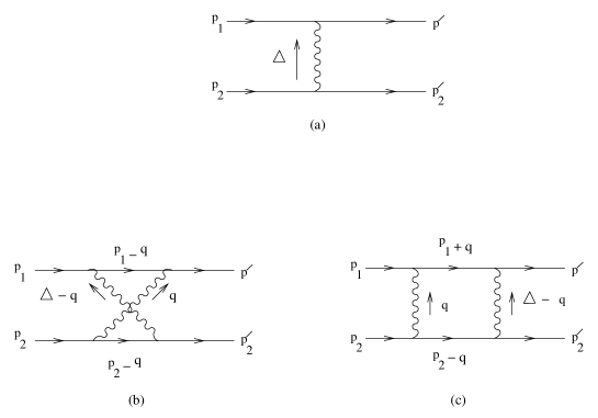
Figure 1: 1 and 2-photon diagrams contributing to the semi classical amplitude in e-e scattering in QED.

The same result as presented above can be succinctly derived from a Feynman diagram approach [2],[3]. This consists of making the necessary high-energy approximations to Feynman graphs, in which, in the eikonal approximation, only ladder type diagrams contribute. These are shown for the cases of $1$, $2$, and $3$-photon exchange in figs. (1), (2).

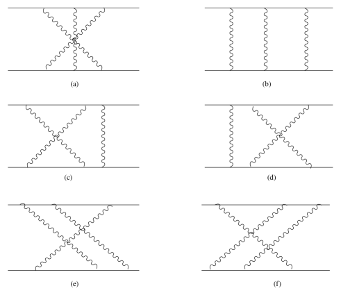
Figure 2: 3-photon diagrams contributing to the semi classical amplitude in e-e scattering in QED.

Consider, for example, the one-photon exchange amplitude. This is simply given by

$${\mathcal{M}}_{1}=\frac{e^{2}s}{2m^{2}}\frac{1}{\bf{\Delta}^{2}+\mu^{2}}$$ (6)

where $e$ is the electron charge, $m$ its mass, and $\bf{\Delta}$ the transverse momentum transfer. A fictitious mass for the photon is included to avoid infra-red divergences. We will assume this mass in all subsequent formulae. Also note that the momentum transfer $\bf{\Delta}$ is assumed to have only transverse components, in line with the limit in which we are working. In Fourier space, (6) can be written as

$${\mathcal{M}}_{1}=-\frac{s}{2m^{2}}\int d^{2}x_{\perp}{\mbox{exp}}\left(i\bf{\Delta}.{\bf x_{\perp}}\right)\left[\frac{e^{2}K_{0}\left(\mu x\right)}{2\pi}\right]$$ (7)

where $x$ is $|{\bf x}_{\perp}|$ and $K_{0}$ is the modified Bessel function. Similarly, one can calculate the amplitude corresponding to figure (2) and the result turns out to be

$${\mathcal{M}_{2}}=\frac{is}{4m^{2}}\int d^{2}x_{\perp}{\mbox{exp}}\left(i\bf{\Delta}.{\bf x_{\perp}}\right)\left[\frac{e^{2}K_{0}\left(\mu x\right)}{2\pi}\right]^{2}$$ (8)

This suggests a beautiful pattern for the general $n$ photon exchange amplitude, and we quote the result here [2],

$${\mathcal{M}_{n}}=-\frac{is}{2m^{2}n!}\int d^{2}x_{\perp}{\mbox{exp}}\left(i\bf{\Delta}.{\bf x_{\perp}}\right)\left[-\frac{ie^{2}K_{0}\left(\mu x\right)}{2\pi}\right]^{n}$$ (9)

And the asymptotic form of the sum of amplitudes with $n$ photon exchange is given by the series

$$\sum_{n=1}^{\infty}{\mathcal{M}}=\frac{is}{2m^{2}}\int d^{2}x_{\perp}{\mbox{e}}^{i{\bf\Delta}.{\bf x_{\perp}}}\left[1-{\mbox{exp}}\left(-\frac{ig^{2}K_{0}(\mu x)}{2\pi}\right)\right]$$ (10)

The integration can be carried out explicitly. Note that since $\mu$ is small, the Bessel function can be expressed as $-\left({\mbox{ln}}\mu x\right)$, and thereafter the integration is standard. The final result is exactly the same as in eq.(5)

We will make a few comments here. First of all, note that the integration is explicitly over the transverse directions only. Hence, in the semi-classical limit, the problem can be thought of as a two-dimensional one. Further, the log that appears in the small argument expression for the Bessel function is strongly reminiscent of the free two dimensional propagator. Therefore, in some sense, one expects that QED in this extreme high energy limit should be described by a free two dimensional theory. In the next subsection, we show that this is indeed the case.

In order to reduce the theory to an effective two-dimensional theory, we need to make certain approximations at the level of the action, which is now commonly known as the Verlindes’ scaling argument. Let us therefore proceed to study this.

2.3 Verlindes’ Scaling Argument

An elegant way of treating high energy scattering is to make simplifications at the level of the action of the theory under considerations [5]. Noting that the square roots of the Mandelstam variables $s$ and $t$ measure the typical momenta associated with the longitudinal and the transverse directions, it is reasonable to associate $two$ length scales, along these two directions, the characteristic length scale along the longitudinal direction being much smaller than that along the transverse direction. Hence we can expect a simplification of the action by performing a rescaling of the coordinates,

$$x^{\alpha}~{} \rightarrow ~{}\lambda x^{\alpha}$$ (11)

$$x^{i}~{} \rightarrow ~{}x^{i}$$ (12)

where $\alpha~{},~{}\beta$ runs over the light cone coordinates $+,~{}-$ and $i$ signifies the space coordinates $x,~{}y$, and $\lambda$ is a scale parameter that we will take to be very small.

The gauge potentials $A^{\mu}$ have the dimension of $(length)^{-1}$ and their transformation property under the rescaling is given by

$$A^{\alpha}~{}\rightarrow~{}\lambda^{-1}A^{\alpha},~{}~{}~{}~{}~{}A^{i}~{}\rightarrow~{}A^{i}.$$ (13)

Performing this scaling in the action, and taking the limit $\lambda\to 0$, we obtain the reduced action

$$S~{}=~{}-{1\over 4}\int d^{4}x\left(\lambda^{-2}F_{\alpha\beta}F^{\alpha\beta}~{}+~{}2F_{\alpha i}F^{\alpha i}\right)$$ (14)

Clearly, in the above action, the dominant contribution comes from configurations with $F_{\alpha\beta}=0$, which can be translated into $E_{z}=0$, thus making contact with the shock wave in eq.(2). This implies the pure gauge condition, $A_{\alpha}=\partial\Omega$, and hence the action (14) can be written as

$$F_{\alpha i}~{}=~{}\left[\partial_{\alpha}\left(A_{i}~{}-~{}\partial_{i}A_{\alpha}\right)\right]$$ (15)

The Euler-Lagrange equation for $A_{i}$ calculated from this action implies that $(A_{i}-\partial_{i}\Omega)$ is a harmonic function, and putting this information back into the action, we obtain a semi-classical value of the action,

$$S~{}=~{}-{1\over 4}\int d^{2}z\int_{-\infty}^{\infty}dx^{+}\partial_{+}\left(A_{i}~{}-~{}\partial_{i}\Omega\right)\int_{-\infty}^{\infty}dx^{-}\partial_{-}\left(A_{i}~{}-~{}\partial_{i}\Omega\right)$$ (16)

From the above equation, it would seem that under a redefinition of our gauge fields via a gauge transformation, we could, in fact, get rid of all local interactions. The important subtlety here is that [5] arbitrary gauge transformations, as suggested by (16), are not allowed at infinity, and that the asymptotic values $\Omega$ should survive. We impose the condition that the transverse gauge field $A_{i}$ take the same values at the two ends of each Wilson line. Then, denoting the asymptotic values of the field $\Omega$ at the end points of the Wilson lines to be $g_{1},g_{2}$ and $h_{1},h_{2}$, and calling $g_{1}-g_{2}=g$ and $h_{1}-h_{2}=h$, we finally obtain the action

$$S~{}=~{}-{1\over 4}\int d^{2}z~{}\partial_{i}g\partial_{i}h$$ (17)

This is thus the free field action for the fields $g$ and $h$ which have dynamics only in the transverse directions, their values in the longitudinal direction being fixed at the asymptotic infinities of the Wilson lines.

It can be shown [7] that the scattering amplitude of two electrons in this high energy limit can be approximated by the expression

$$f(s,t)=\frac{is}{2m^{2}}\int d^{2}z{\mbox{e}}^{iq.z}\left<V_{+}(z)V_{-}(0)\right>$$ (18)

where $V_{\pm}$ are the Wilson lines defined by

$$V_{\pm}~{}=~{}{\mbox{exp}}\left(e\int_{-\infty}^{\infty}dx^{\pm}A_{\pm}(z)\right)$$ (19)

$e$ denoting the charge of the particles. Carrying out the integrations explicitly, we see that the scattering amplitude reduces to

$$f(s,t)~{}=~{}\frac{is}{2m^{2}}\int d^{2}z{\mbox{e}}^{iq.z}~{}\left<{\mbox{e}}^{g}~{}{\mbox{e}}^{h}\right>$$ (20)

Now, using $\left<{\mbox{e}}^{g}{\mbox{e}}^{h}\right>={\mbox{e}}^{\left<gh\right>}$, and noting that the propagator in two dimensions is a log, we obtain

$$f(s,t)~{}=~{}\frac{is}{2m^{2}}\int d^{2}z{\mbox{e}}^{iq.z}~{}{\mbox{e}}^{-\frac{ie^{2}}{4\pi}ln|z|}$$ (21)

The integration can be performed in the same way as in the last subsection and again yields the same result as in eq.(5).

Let us briefly summarise what we have obtained till now. We have described three different ways of calculating the ultra-high energy scattering amplitude for two electrons. The first method involved a semi-classical calculation, where one of the electrons was boosted to the speed of light and the change in the wave function of the other was calculated (in the frame in which the second electron is at rest). The second method involved approximations in the Feynman diagrams of QED, and the third involved truncating the full QED action in order to obtain an effective two-dimensional free field theory.

Before proceeding further, let us point out that the shock wave picture has been studied in great details in the context of gravitational Planckian scattering. See, for eg. [8],[9].

We are now ready to discuss the same scenario in the context of non-commutative QED (NCQED), i.e QED in non-commutative spaces. This has received a lot of attention of late [10], following the motivation of such spaces from the point of view of string theory [11]. We will be interested in calculating the scattering amplitudes of two electrons in non-commutative space. Our main motivation for doing so is the formal similarity between NCQED and QCD. It is well known, that NCQED has three and four-photon interactions, which are absent in usual QED. One might, therefore, be tempted to think that the high-energy scattering behaviour of NCQED would in some sense, be similar to that of QCD. The latter has been well studied in [2] and one of the main results therein is the appearance of logarithmic factors of the centre of mass energy in the scattering amplitude, which are absent in QED upto sixth order in the coupling. Further, it has been shown that in this energy regime, the gluon exhibits Regge behaviour, while the photon doesnt. We would like to understand the same phenomena in the context of NCQED , which is our topic of study in the next section.

3 High Energy Scattering in Non-Commutative QED

We now address the question of high-energy scattering in NCQED. Our hope here is that there would be some features which are qualitatively different from those in usual QED, because of the widely different natures of these two theories (the Feynman rules for NCQED are presented in the appendix). For earlier work on scattering in non-commutative theories, see, for eg., [12].

3.1 The Fate of The Shock Wave

First of all, we would like to understand the nature of the “shock wave” in NCQED . Here, we run into an obvious problem. Due to the lack of Lorentz invariance in the theory, the results for the scattering amplitude are expected to be frame dependent, and although, one could, in principle, boost one of the charges, the semiclassical approach is expected to be difficult in this case, due to the non-linearity of the noncommutative theory and indeed, the shock wave picture ceases to be valid, as will be made clearer in a while. Note that we could, however, try and apply the other two procedures that we have outlined. Namely, we could make approximations at the level of Feynman diagrams for NCQED , and we could scale the action, as is appropriate for such high energy scattering. Let us study the second procedure first. We will argue non-commutative corrections invalidate the shock wave picture.

Let us begin by noting that the non-commutative generalisation of the free Maxwell action is to replace the usual product by the star product and expressing the field strength in terms of the gauge potential ${\hat{A}_{\mu}}$.

$${\mathcal{L}} = -\frac{1}{4}{\hat{F}_{\mu\nu}}\star{\hat{F}^{\mu\nu}}$$

$${\hat{F}_{\mu\nu}} = \partial_{\mu}{\hat{A}_{\nu}}-\partial_{\nu}{\hat{A}_{\mu}}-ie\left({\hat{A}_{\mu}}\star{\hat{A}_{\nu}}-{\hat{A}_{\nu}}\star{\hat{A}_{\mu}}\right)$$ (22)

The star product here is defined by

$$\left(\Phi_{1}\star\Phi_{2}\right)(x)=\left[{\mbox{exp}}\left(\frac{i}{2}\theta^{\alpha\beta}\partial_{\alpha}\partial^{\prime}_{\beta}\right)\Phi_{1}(x)\Phi_{2}(x^{\prime})\right]_{x=x^{\prime}}$$ (23)

and we define the Moyal bracket as

$$\left[A_{\mu},A_{\nu}\right]_{MB}=A_{\mu}\star A_{\nu}-A_{\nu}\star A_{\mu}$$ (24)

Using the Seiberg-Witten map that expresses the non-commutative gauge fields and gauge parameters in terms of the commutative ones order by order in $\theta$, [11], the Lagrangian of the theory (upto first order in $\theta$), is given by [13]

$$\mathcal{L}=-\frac{1}{4}F_{\mu\nu}F^{\mu\nu}+\frac{1}{8}\theta^{\alpha\beta}F_{\alpha\beta}F_{\mu\nu}F^{\mu\nu}-\frac{1}{2}\theta^{\alpha\beta}F_{\mu\alpha}F_{\nu\beta}F^{\mu\nu}+O\left(\theta^{2}\right)$$ (25)

Let us consider very high energy scattering in NCQED using this Lagrangian. We assume, without loss of generality that the components of $\theta$ are non-vanishing only along the transverse directions, i.e $\theta^{12}=-\theta^{21}=\theta$. It has been shown that for time like non-commutativity, the theory is often non-unitary [14] and we will not be concerned with such aspects for the purpose of this paper.

Note that $\theta$ has the dimensions of the square of the transverse length and its scale is fixed accordingly. In particular, following [5], we set the length scale of the longitudinal directions to be $\lambda<<1$ and that of the transverse dimensions to unity. Hence, in the action, $\theta$ is not scaled. We are, in a sense, making the simplifying assumption that $\theta$ does not set a new scale in the theory. In what follows, we will show that even with this limitation, it is clear that the usual shock wave picture of high-energy scattering in QED is invalidated. Scaling the action as in [5], we obtain the leading term in the Lagrangian (equivalent to the first term in eq.(14) as

$$\frac{1}{\lambda^{4}}F^{\alpha\beta}\left[-{1\over 4}F_{\alpha\beta}+\frac{1}{8}\theta^{ij}F_{ij}F_{\alpha\beta}F^{\alpha\beta}-{1\over 2}\theta^{ij}F_{\alpha i}F_{\beta j}F^{\alpha\beta}\right]$$ (26)

Expressing the field strength in terms of the electric and magnetic fields in the usual way, we find that the dominant contribution to the path integral comes from configurations in which

$$E_{z}=-\theta^{12}\left(E_{x}B_{x}+E_{y}B_{y}\right)$$ (27)

This result, which is valid in any frame of reference in which the longitudinal momentum is very large compared to the transverse ones (in particular the centre of mass frame) is the NCQED analogue of the shock wave picture of the last section. From eq.(27), it is clear that the interaction between two electrons moving at ultra-high energies is no longer instantaneous in this framework. The non-vanishing $E_{z}$ causes the two particles to interact at all times, and hence the simple calculations of the last section can no longer be performed here.

The same result can be obtained by starting with the pure non-commutative Maxwell action, eq. (22), and noting that in terms of this action, the scaling argument produces the pure gauge condition in NCQED , ${\hat{F}}_{\alpha\beta}=0$ where

$${\hat{F}}_{\alpha\beta}=\partial_{\alpha}A_{\beta}-\partial_{\beta}A_{\alpha}-ie\left[A_{\alpha},A_{\beta}\right]_{MB}$$ (28)

and on the r.h.s we have the Moyal bracket of the gauge fields. Expanding the r.h.s to leading order in $\theta$, this equation gives the same condition as eq.(27).

It is difficult, in this framework, to estimate the corrections to the usual QED amplitudes for NCQED . As we have already seen, the shock-wave picture is not valid in this framework (at least in the centre of mass frame) and an effective way to calculate the NCQED corrections to the shock wave using semi-classical techniques is not known to the present authors. The problem arises because of the fact that the dispersion relations in NCQED are non-linear [15] and it is difficult to solve this set of Maxwell’s equations explicitly.

Therefore, we are led naturally to the approach (2) described in the last section. Namely, we would make approximations in the Feynman diagrams for NCQED in the high energy limit, in order to evaluate the corrections. Naively, it might seem that these corrections will be negligible, since we have tuned the non-commutativity parameter $\theta$ to take values only in the transverse directions. As we will now show, this is not true. It turns out that there are in fact important leading log corrections to the high-energy scattering amplitude in NCQED .

A simple way to understand this is as follows. Consider the usual QED. It is well known [2] that in this theory, there are no leading log corrections to electron-electron scattering upto the sixth order. At the eighth order, such corrections start appearing as a result of uncancelled logarithms arising due to electron loops inside ladder diagrams. The cancellation of the leading logs (upto sixth order) can be seen most easily by the method of “flow diagrams.” This technique was invented in [2] in order to keep track of the factors that contains the logarithms of the centre of mass energy in the high-energy limit. It turns out that in QED, although all the individual diagrams have such logarithmic factors, these are cancelled when one sums all diagrams, and hence the absence of leading logs upto sixth order.

The logarithmic factors appear in the individual QED diagrams, as an infrared cutoff to the longitudinal momenta. For NCQED, since we have chosen the directions of noncommutativity to be along the transverse directions, these logarithms will appear as in usual QED. However, we expect the scenario to be modified in the context of NCQED because of two reasons. Firstly, the Feynman rules for NCQED contains extra phases, (which, in our case depend only on transverse momenta), and which might be different for different diagrams. Hence the leading logs might not cancel. The second reason for which we might expect leading logs in NCQED amplitudes is because of the QCD like processes involving three and four photon interactions (fig. (3). Let us therefore proceed to study these in some details.

3.2 Feynman Diagram Calculations for NCQED

To be specific, we will, in the spirit of our QED discussion, consider only multi-photon exchange diagrams of QED and the QCD-like corrections to the same in NCQED , upto the sixth order, as in figures (1) and (2). This will bring us to the issue of the leading corrections to the eikonal picture that we have described in section 2.

Of course, this set of diagrams is not exhaustive, and there are other diagrams to the same orders that we are considering, like radiative corrections to the form factors, etc. These diagrams will be important in modifying the vertex functions and the photon propagator [2]. These will bring in the important issues of renormalisation and the UV/IR mixing phenomena in non-commutative gauge theories [16],[17]. For the purpose of this paper, we do not consider these diagrams further, and assume that as in the case of usual QED, the behaviour of these in the high energy limit will not modify our results on the logarithmic factors of the centre of mass energy. As we have already pointed out, the logarithmic factors of $s$ appears in our calculations as infrared cutoffs for the longitudinal momenta (see Appendix) and the non-commutative parameter $\theta$ will be set to zero along these directions. Hence, in a sense, we expect these factors of ${\mbox{log}}(s)$ to remain unaffected in NCQED . It will indeed be interesting to compute the radiative corrections to the fermion form factors in the high-energy limit in NCQED , and we will leave this to a future work.

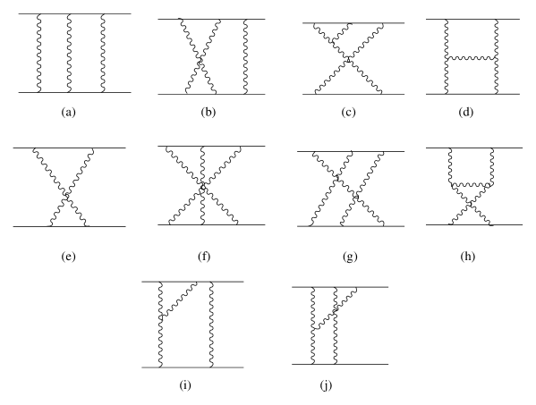
Figure 3: sixth order interaction diagrams that contribute in e-e scattering in NCQED.

Let us first specify the regimes of our calculation. We will be working in the centre of mass frame, and will use the usual Mandelstam variables, $s$, $t$ and $u$. We will work in the almost forward regime, where $t<<s$. It turns out that the calculations become simple if we choose the $\theta$ regime to be

$$\theta t=\theta\bf{\Delta}^{2}<<1$$ (29)

where $\theta$ is the non-commutativity parameter. Hence, we will be working in the regime of small $\theta$.

We will be using the method of flow diagrams as in [2] (see also [18]). We will not elaborate on this method here (a brief review is contained in the Appendix), but let us point out some salient features of this technique. It consists of properly choosing the poles of the propagators in the Feynman diagrams, such that the loop integrals are simplified. In order to achive this, one draws all possible flow diagrams indicating the possible directions of the negative components of the loop momenta. Integration over the positive components (in the light cone sense) is then carried out, using the residue theorem, and integration over the $(-)$ components of the loop momenta are seen to produce the log factors in the diagram.

Let us now consider the second and fourth order diagrams in NCQED in the extreme high energy limit. Consider first the second order diagram, depicted in fig (1). In the centre of mass frame, the incoming and outgoing momenta have only longitudinal components, whereas the parameter $\theta$ has only transverse components in our scenario. Hence, the phase factor can be seen to be unity. Let us now consider the fourth order diagrams. There are two of them, as in fig. (1), and each of them has one flow diagram, which is the same as the labelling of momenta shown. Using the same arguments as before, we find that in diagram (b) of fig. (1), the net phase factor is ${\mbox{exp}}(i\bf{q_{\perp}}\times\bf{\Delta})$ while for diagram (c) of fig. (1), the phase factor is unity. The logarithmic factors for the amplitudes for these diagrams, including the phase factors are respectively,

$${\mathcal{M}}_{a}=-\frac{e^{4}s{\mbox{ln}}s}{4\pi m^{2}}\int\frac{d^{2}q_{\perp}}{(2\pi)^{2}}\frac{{\mbox{e}}^{i\bf{q_{\perp}}\times\bf{\Delta}}}{\left({\bf q_{\perp}}^{2}\right)\left[\left(\Delta-{\bf q_{\perp}}\right)^{2}\right]}~{}=~{}-\frac{e^{4}s{\mbox{ln}}s}{4\pi m^{2}}I^{\prime}\left(\bf{\Delta}\right)$$

$${\mathcal{M}}_{b}=\frac{e^{4}s{\mbox{ln}}s}{4\pi m^{2}}\int\frac{d^{2}q_{\perp}}{(2\pi)^{2}}\frac{1}{\left({\bf q_{\perp}}^{2}\right)\left[\left(\Delta-{\bf q_{\perp}}\right)^{2}\right]}~{}=~{}\frac{e^{4}s{\mbox{ln}}s}{4\pi m^{2}}I\left(\bf{\Delta}\right)$$ (30)

Where $I^{\prime}$ and $I$ are the integrals with and without the phase factors respectively. The term proportional to ${\mbox{ln}}s$ is now

$${\mathcal{M}}=-\frac{e^{4}s{\mbox{ln}}s}{4\pi m^{2}}\int\frac{d^{2}q_{\perp}}{(2\pi)^{2}}\frac{{\mbox{cos}}\left(\bf{q_{\perp}}\times\bf{\Delta}\right)-1}{\left({\bf q_{\perp}}^{2}\right)\left[\left(\Delta-{\bf q_{\perp}}\right)^{2}\right]}$$ (31)

and the usual QED amplitude, without the logs is now modified (under a Fourier transform to position space) to

$${\mathcal{M}}=\frac{ie^{4}s{\mbox{ln}}s}{2\pi m^{2}}\int d^{2}x{\mbox{e}}^{i\bf{\Delta}.\bf{x_{\perp}}}K_{0}\left(\lambda|\bf{x_{\perp}}|\right)K_{0}\left(\lambda|\bf{x_{\perp}}^{\prime}|\right)$$ (32)

where $\bf{x_{\perp}}^{\prime}=\sqrt{\bf{x_{\perp}}^{2}+\left(\theta\bf{\Delta}\right)^{2}+\left(\bf{x_{\perp}}\times\bf{\Delta}\right)}$. It is interesting to note that one of the coordinates have been shifted by a term proportional to $(\theta\bf{\Delta})$.

The $\theta~{}=~{}0$ case corresponds to these amplitudes in usual QED [2], and in this case, the integrals cancel each other.

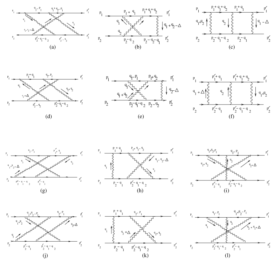
Figure 5: Flow diagrams contributing to the sixth order amplitude in e-e scattering. Each of the diagrams in (2) has two flow diagrams, which have been depicted in the figure with appropriate labelling.

Now let us consider the sixth order amplitudes in NCQED. Some of the relevant diagrams have been depicted in fig.(2). It is well known [2] that Each of these diagrams have two flow diagrams, which we have presented in the appendix, in figure (5). Consider fig. (2). In order to evaluate these diagrams, it is sufficient to calculate only two of them, (b) and (d). This is because (b) is related by $s\to u$ to (a). (c) and (d) line 2 are equal, and are related by $s\to u$ to those on line 3.

The phase factors for these diagrams can be easily determined by the flow diagrams in fig. (5). The important point to note here is that not all the diagrams have similar phase factors. For eg. the diagrams of the middle column have unit phase factors, and so have the lower two diagrams of the last column. All the other diagrams have non-vanishing phase factors.

A small comment is in order here. It is known that these diagrams often have ${\mbox{ln}}^{2}s$ terms, which are known to cancel in commutative QED. It can be shown that the same happens in the case of NCQED too, and that there are no such terms in the amplitude. We now list the expressions for the amplitudes in figure (2). Using the notation

$$I_{1}=\int\prod_{i=1}^{3}\frac{d^{2}q_{i\perp}}{(2\pi)^{2}}{\mbox{cos}}\left(\bf{q_{1\perp}}\times\bf{q_{2\perp}}\right)\frac{(2\pi)^{2}\delta^{(2)}\left(\sum_{i=1^{3}}{\bf q_{i\perp}}-\bf{\Delta}\right)}{\prod_{i=1}^{3}\left({\bf q_{i\perp}}^{2}+\mu^{2}\right)}$$ (33)

$$I_{2}={1\over 2}\int\prod_{i=1}^{2}\frac{d^{2}q_{i\perp}}{(2\pi)^{2}}{\mbox{cos}}\left(\bf{q_{1\perp}}\times\bf{q_{2\perp}}\right)\frac{{\mbox{ln}}~{}\frac{{\bf q}_{2\perp}^{2}}{{\bf q}_{1\perp}^{2}}\left({\bf q}_{2\perp}^{2}+{\bf q}_{1\perp}^{2}\right)}{\left({\bf q}_{1\perp}^{2}\right)^{2}\left({\bf q}_{2\perp}^{2}\right)^{2}\left({\bf q}_{1\perp}^{2}-{\bf q}_{1\perp}^{2}\right)\left({\bf q}_{1\perp}+{\bf q}_{2\perp}+\bf{\Delta}\right)^{2}}$$ (34)

and the values of these integrals for $\theta=0$ by $I_{1}^{\prime}$ and $I_{2}^{\prime}$ respectively, the amplitudes are given by

$${\mathcal{M}}_{a+b} = -\frac{e^{6}s{\mbox{ln}}s}{2\pi^{2}m^{2}}\left[I_{2}+I_{2}^{\prime}\right]~{}~{}~{}~{}{\mbox{row 1}}$$

$${\mathcal{M}}_{c+d} = \frac{e^{6}s{\mbox{ln}}s}{2\pi^{2}m^{2}}\left[I_{2}^{\prime}+i\pi I_{1}^{\prime}\right]~{}~{}~{}~{}{\mbox{row 2}}$$

$${\mathcal{M}}_{e+f} = \frac{e^{6}s{\mbox{ln}}s}{2\pi^{2}m^{2}}\left[I_{2}-i\pi I_{1}\right]~{}~{}~{}~{}{\mbox{row 3}}$$ (35)

For the case $\theta~{}=~{}0$, the sum of the above terms reduces to zero, signifying that there are no logarithmic factors of energy in the sixth order e-e scattering in QED. In this case, however, the sum is non-zero, and given by

$${\mathcal{M}}_{6}=-\frac{ie^{6}s{\mbox{ln}}s}{2\pi m^{2}}\int\prod_{i=1}^{3}\frac{d^{2}q_{i\perp}}{(2\pi)^{2}}\left[{\mbox{cos}}\left(\bf{q_{1\perp}}\times\bf{q_{2\perp}}\right)-1\right]\frac{(2\pi)^{2}\delta^{(2)}\left(\sum_{i=1^{3}}{\bf q_{i\perp}}-\bf{\Delta}\right)}{\prod_{i=1}^{3}\left({\bf q_{i\perp}}^{2}+\mu^{2}\right)}$$ (36)

and hence there is a logarithmic contribution at sixth order, which is imaginary in nature.

Now, we will consider QCD like corrections in NCQED. In fig. (3), we have drawn a few of the sixth order diagrams that will contribute to the scattering process. The rest of these diagrams can be obtained by reflections along a horizontal or a vertical line. For example, in fig. (3), diagrams (a), (b), (f), (g) and their permutations are the QED-like contributions of fig. (2). The remainder of the diagrams in fig (3) are the novel diagrams of NCQED , and contribute to the sixth order process. There are fifteen such diagrams, which can be obtained as reflections of those presented here. For example, there are four diagrams corresponding to (c) in fig. (3), obtained from (c) by reflections about a vertical or horizontal line. These are, of course all equal.

Note that the four photon vertex in diagram (e) of fig. (3) can be thought of as the fused diagrams corresponding to (d) and (h). We will follow [2] and add the contribution of (e) to (d) and (h) before we make the asymptotic calculation. The integrals in the expressions to follow will be of two types.

$${\tilde{I}}_{1}=\int\prod_{i=1}^{2}\frac{d^{2}q_{i\perp}}{(2\pi)^{2}}{\mbox{sin}}^{2}\left(\bf{q_{1\perp}}\times\bf{q_{2\perp}}\right)\frac{\bf{q_{1\perp}}^{2}+\bf{q_{2\perp}}^{2}}{\prod_{i=1}^{2}\bf{q_{i\perp}}^{2}\left(\bf{\Delta}-\bf{q_{i\perp}}\right)^{2}}$$

$${\tilde{I}}_{2}=\int\prod_{i=1}^{2}\frac{d^{2}q_{i\perp}}{(2\pi)^{2}}{\mbox{sin}}^{2}\left(\bf{q_{1\perp}}\times\bf{q_{2\perp}}\right)\frac{\bf{\Delta}^{2}}{\prod_{i=1}^{2}\bf{q_{i\perp}}^{2}\left(\bf{\Delta}-\bf{q_{i\perp}}\right)^{2}}$$ (37)

The integral ${\tilde{I}}_{1}$ is an ultra-violet divergent integral. In usual QCD, the terms proportional to ${\tilde{I}}_{1}$ cancel, when we arrange the diagrams with the appropriate group theory factors, but this cancellation is not seen here. It would be tempting to argue that these ultraviolet divergences would disappear in the renormalised theory, but we do not have a concrete proof of the same. We leave this issue for a future study, and for the moment we list the results for the QCD-like diagrams of fig. (3). First, we list the terms that depend on ${\tilde{I}}_{1}$.

$${\mathcal{M}}_{d+e+h}^{{\tilde{I}}_{1}} = 4\frac{e^{6}s}{8\pi^{2}m^{2}}\left[{\mbox{ln}}\left(se^{i\pi}\right)\right]^{2}{\tilde{I}}_{1}-4\frac{e^{6}s}{8\pi^{2}m^{2}}\left[{\mbox{ln}}s\right]^{2}{\tilde{I}}_{1}$$

$${\mathcal{M}}_{j}^{{\tilde{I}}_{1}} = -2\frac{e^{6}s}{8\pi^{2}m^{2}}\left[{\mbox{ln}}\left(se^{i\pi}\right)\right]^{2}{\tilde{I}}_{1}+2\frac{e^{6}s}{8\pi^{2}m^{2}}\left[{\mbox{ln}}s\right]^{2}{\tilde{I}}_{1}$$

$${\mathcal{M}}_{c+i}^{{\tilde{I}}_{1}} = -2\frac{e^{6}s}{8\pi^{2}m^{2}}\left[{\mbox{ln}}\left(se^{i\pi}\right)\right]^{2}{\tilde{I}}_{1}-2\frac{e^{6}s}{8\pi^{2}m^{2}}\left[{\mbox{ln}}s\right]^{2}{\tilde{I}}_{1}$$

The contribution to these diagrams in the form of $I_{2}$ comes only from diagrams (d),(e) and (h) and is given by the expression

$${\mathcal{M}}_{d+e+h}^{{\tilde{I}}_{2}}=-i\frac{e^{6}s}{8\pi m^{2}}\left[{\mbox{ln}}s\right]{\tilde{I}}_{2}$$ (39)

The sum of the QCD like contributions is thus given by

$${\mathcal{M}}_{QCD-like}~{}=~{}-4\frac{e^{6}s}{8\pi^{2}m^{2}}\left({\mbox{ln}}s\right)^{2}{\tilde{I}}_{1}-\frac{ie^{6}}{8\pi m^{2}}\left(s{\mbox{ln}}s\right){\tilde{I}}_{2}$$ (40)

Note that the second term on the r.h.s of eq. (40) is formally similar to the expression in eq. (36), but in the former, the integrand is proportional to $\bf{\Delta}^{2}$, which we have assumed to be very small, and hence the ${\mbox{log}}s$ contribution coming from (36) dominates. In the above calculations of the fourth and sixth order processes, we have neglected terms proportional to $\bf{\Delta}\theta$ in the phase factors. These will provide subleading corrections to our results.

Our calculations above clearly show that for ultra-high energy scattering in NCQED , there are novel effects. The usual QED amplitude is corrected by leading logarithms. Although these logarithms appear at the sixth order in perturbation theory, it is possible that they will be significant in comparing with experimental predictions of NCQED .

4 Discussions and Conclusions

In this paper, we have studied almost-forward scattering in the context of NCQED . We have shown that even in this regime where the kinematics make the theory extremely simple, there is a difference between NCQED and usual QED. The difference arises expectedly because of the non-commutative nature of space, and even at the semi classical level, we have shown that the two theories exhibit completely different natures. Whereas in commutative QED, the shock wave picture can be effectively used to calculate scattering amplitudes exactly, the same fails for the case of NCQED . As we have seen, the difference arose because in NCQED , the interaction between two fast moving particles become non-local in the longitudinal directions.

Further, we have shown that in NCQED , using Feynman diagram techniques to calculate the amplitude perturbatively yields vastly different results from QED, and that there appear logarithmic factors of energy in the amplitude from the sixth order. In usual QED, these factors in fact cancel out when one adds the diagrams. For the QED like diagrams in NCQED , they do not, since the diagrams come with different phase factors. Further, the QCD like diagrams in NCQED produce terms of the order of ${\mbox{ln}}^{2}s$.

We have not considered the effects of renormalisation of NCQED in this paper, and in particular the peculiarities like the UV/IR mixing encountered in the same. We have assumed, in a sense, that these issues will not modify our results on the leading logarithms. One way to see this is to note that in usual QED, the diagrams that are not of the ladder type are all of the order of $s$, and do not affect the leading log behaviour. It will be interesting to study this issue in some details, and we leave this to a future publication.

Further, it would be interesting to see if there exists an effective two dimensional theory of high energy scattering in NCQED in lines with our discussion of section 2. One would be tempted to think that the asymptotic behaviour of the amplitudes in NCQED would be similar to those of QED but with usual products replaced by star products. This is, in general, a complicated problem to tackle, because many of the simplifying assumptions of QED will not be valid in this case, since different diagrams appear with different phase factors. However, it seems to us that even in NCQED , the scattering amplitude can be calculated as the expectation value of two Wilson lines, as in section 2. It might be possible to calculate the logarithmic factors presented in this paper from a two-dimensional field theory point of view.

Also, it would be interesting to compute the corrections to our picture. We have made the simplifying assumption that $\theta$ is very small compared to the centre of mass energy. It would be of interest to estimate the leading order correction terms. It is then that we hope to be able to connect to experimental results. We leave these issues to a future work.

Acknowledgements

It is a pleasure to thank G. Thompson for several helpful discussions and comments and for a careful reading of the manuscript. We would like to thank Sumit Das for his comments on the manuscript. We thank N. Mahajan for helpful correspondence. We also thank L. Bonora, Venkat Pai, and A. Sen for discussions. T. S would like to thank T. Jayaraman who had introduced him to this subject. Z. A would like to thank all the members of the ICTP high energy group for their encouragement and support.

Appendix

In this appendix, first we briefly review the method of flow diagrams that we have used in section 3. Then, we present the Feynman rules for NCQED . Finally, we draw the flow diagrams for the sixth order QED-like diagrams for NCQED .

Appendix A Flow Diagrams

The calculations of Feynman diagrams for high energy scattering are considered to be difficult, but they are actually quite easy even for higher orders diagrams. The mathematical expression for a higher order diagram is of course long but because of high energy center of mass momenta approximations they can be calculated easily in a systematic way.

A Feynman amplitude can be written either over loop momenta or we can introduce Feynman parameters and then perform the integration over momenta variables. The asymptotic behaviour of Feynman amplitudes in the high energy limit is obtained by making approximations in either method. Historically, the high energy approximation was first made in Feynman parameter formulation. This method is rigorous but lengthy and intermediate steps are complicated but the final asymptotic expressions are quite simple. This shows that there is a relatively easy way to to get final results. The approximation in momenta variables achieves this. First of all, this approximation in momentum variables was employed by Sudakov [19] and we also use momentum variables to study high energy behaviour of scattering in gauge field theories.

We study the scattering process in center of mass frame in such a way that the spatial momenta of the two incident particles are along the positive z direction and negative z direction, with magnitude $w_{1}$ and $w_{2}$ respectively. In order to calculate the Feynman amplitude for a given diagram, we first perform the integratin over the plus momenta explicitly by contour integration, and then the integration over minus momenta is performed by making suitable approximations.

This later integration may be infinite if we set $s$, (the square of the center of mass energy) to be infinite. This divergence is logarithmic. In some diagrams we may find a divergence which is more than logarithmic but in gauge field theories such divergence usually cancel when we sum all diagrams of a given order of perturbation. So the Feynman amplitude is proportional to $lns$ and the integrals over transverse momenta. There may be divergence from a single diagram arising from this transverse momenta integration but again such divergences generally vanish when we sum over all diagrams of a given perturbation order.

Appendix B The Box Diagram

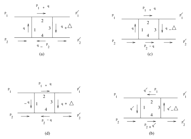
Figure 4: The flow diagrams corresponding to the box diagram (b) of fig. (1). Only diagram (c) contributes.

Let us illustrate this in some details. Consider the box diagram in fig. (4). We assume, for simplicity, that the solid lines represent scalar particles. Take the propagator of momentum q. In light coordinates we can write the denominator of this propagator as

$$q_{+}q_{-}+q_{\perp}^{2}+m^{2}+i\epsilon$$ (41)

This propagator has one pole locatedd at

$$q_{+}=-\frac{q_{\perp}^{2}+m^{2}}{q_{-}}-\frac{i\epsilon}{q_{-}}$$ (42)

This pole is located in lower half plane if $q_{-}$ is positive and if $q_{-}$ is negative, then this pole is in upper half plane. For a given Feynman diagaram there is no restriction on value of $q_{-}$ momenta, it can be positive or negative. There are two different regions of kinematics belonging to the two different value of $q_{-}$ momentum. We represent this by the two diagrams in fig. (4), (b) and (c). These are known as the flow diagrams. By definition minus momenta is positive in a flow diagram. In diagram (b) of fig. (4), $q_{-}^{{}^{\prime}}=-q_{-}$. Now the minus momenta of lines 2,3 and 4 can take positive or negative values, so more flow diagrams must be drawn to show these possibilities. Here, we make an approximation by setting $p_{1-}$ and $p_{1-}{{}^{\prime}}$ to 0. This approximation is justified only in the calculation of leading logarithms. Then the conservation of minus momenta applies that the direction of arrows on lines 1,2 and 3 must not be changed. Finally we have four flow diagrams for a box diagram. Diagram (d) is not allowed because at lower left vertex all the momenta are going in. In diagram (a), all the four arrows are in same direction so in each propagator the loop momenta $q>0$. This implies that all the four poles belonging to each porpagator lies in lower half plane and if we enclose our contour by upper half plane contribution from this diagram is zero, same reason holds for diagram (b). For fig (c), the situation is different. Arrows on lines 1,2 and 3 are in the same direction but the arrow on line 4 is in opposite direction to other three lines. Hence, only (c) contributes to the scattering amplitude corresponding to the box diagram.

In diagram (c), the poles of line 1,2 and 3 lies in lower half plane but the pole of line 4 with propagator ${P_{2}-q}^{2}+i\epsilon$ lies in the upper half plane as we can see from sign of q. For flow diagram (a), either we can enclose the lower three poles or the upper one pole and it is easier to enclose one pole. Now, the scattering amplitude can be easily calculated. We label the momenta as $p_{1}=\left(\omega,0,0,\omega\right)$ and $p_{1}=\left(\omega,0,0,-\omega\right)$ in the centre of mass frame, so that the light cone momenta $p_{1-}=p_{2+}=0$, and denoting $q_{-}=2\omega x$, where the values of $x$ are specified to lie between $0$ and $1$ from the conditions of positivity of line momenta along the arrows of diagram (c). For the line of momentum $(-p_{1}^{\prime}+q)^{2}-m^{2}$, the denominator can be easily seen to be $sx$. Now, integration over the variable $x$ (which replaces the integration over $q_{-}$ will produce the desired factor of ${\mbox{log}}s$, if we cut off the $q_{-}$ integration to the order $\frac{1}{s}$. The final answer is

$${\mathcal{M}}_{box}=-\frac{g^{4}s{\mbox{ln}}s}{4\pi}\int\frac{d^{4}q}{{(2\pi)}^{4}}\frac{1}{\left(\bf{q_{\perp}}\right)^{2}\left(\bf{q_{\perp}}-\bf{\Delta}\right)^{2}}$$ (43)

References

- [1] R. Jackiw, D. Kabat, M. Ortiz, “Electromagnetic fields of a massless particle and the eikonal,” Phys. Lett. B 277 (1992) 148, hep-th/9112020.
-
[2]
There has been enormous work done on this subject in the 60’s and 70’s. Due to
its sheer volume, all the references cannot be included here. A good list of these
can be obtained in the book by
H. Cheng, T. T. Wu, “Expanding Protons: Scattering at High Energies,”
M.I.T Press, Cambridge, Ma, 1987, which also adopts a more modern notation than
those of several of the original works. For a sample of the initial work in
this direction, the reader is referred to
H. Cheng and T. T. Wu, “High-Energy Elastic Scattering In Quantum Electrodynamics,” Phys. Rev. Lett. 22 (1969) 666
H. Cheng and T. T. Wu, “Inelastic Electron Scattering At High Energies,” Phys. Rev. Lett. 22 (1969) 1409
H. Cheng and T. T. Wu, “High-Energy Collision Processes In Quantum Electrodynamics. I,” Phys. Rev. 182 (1969) 1852
H. Cheng and T. T. Wu, “High-Energy Collision Processes In Quantum Electrodynamics. II,” Phys. Rev. 182 (1969) 1868
H. Cheng and T. T. Wu, “High-Energy Collision Processes In Quantum Electrodynamics. III,” Phys. Rev. 182 (1969) 1873
H. Cheng and T. T. Wu, “High-Energy Collision Processes In Quantum Electrodynamics. IV,” Phys. Rev. 182 (1969) 1899
H. Cheng and T. T. Wu, “Logarithmic Factors In The High-Energy Behavior Of Quantum Electrodynamics,” Phys. Rev. D 1 (1970) 2775
B. M. Mccoy and T. T. Wu, “Comment On High-Energy Behavior Of Nonabelian Gauge Theories,” Phys. Rev. Lett. 35 (1975) 604
B. M. McCoy and T. T. Wu, “Fermion - Fermion Scattering In A Yang-Mills Theory At High-Energy: Sixth Order Perturbation Theory,” Phys. Rev. D 12 (1975) 3257. - [3] H. D. I. Abarbanel, C. Itzykson, “Relativistic Eikonal Expansion,” Phys. Rev. Lett. 23 (1969) 53.
- [4] E. Meggiolaro, “A Remark on the high-energy quark-quark scattering and the eikonal approximation,” Phys. Rev. D53 (1996) 3835, hep-th/9506043.
- [5] E. Verlinde, H. Verlinde, “QCD at high-energies and two-dimensional field theory,” hep-th/9302104.
- [6] E. Verlinde and H. Verlinde, “Scattering at Planckian energies,” Nucl. Phys. B 371 (1992) 246, hep-th/9110017.
- [7] O. Nachtmann, “Considerations Concerning Diffraction Scattering in Quantum Chromodynamics,” Annals of Physics, 209 (1991) 436.
- [8] G. ’t Hooft, “Graviton Dominance In Ultrahigh-Energy Scattering,” Phys. Lett. B198 (1987) 61.
-
[9]
S. Das and P. Majumdar,
“Charge - Monopole Versus Gravitational Scattering At Planckian Energies,” Phys. Rev. Lett. 72 (1994) 2524 hep-th/9307182.
“Electromagnetic and gravitational scattering at Planckian energies,” Phys. Rev. D51 (1995) 5664 hep-th/9411061.
“Eikonal Particle Scattering and Dilaton Gravity,” Phys. Rev. D55 (1997) 2090 hep-th/9512209. -
[10]
See, for eg.
M. Hayakawa, “Perturbative analysis on infrared aspects of noncommutative QED on R**4,” Phys. Lett. B478 (2000) 394 hep-th/9912094,
M. Hayakawa, “Perturbative analysis on infrared and ultraviolet aspects of noncommutative QED on R**4,” hep-th/9912167,
F. Ardalan and N. Sadooghi, “Axial anomaly in non-commutative QED on R**4,” Int. J. Mod. Phys. A16 (2001) 3151 hep-th/0002143,
L. Alvarez-Gaume and J. L. Barbon, “Non-linear vacuum phenomena in non-commutative QED,” Int. J. Mod. Phys. A16 (2001) 1123 hep-th/0006209,
I. F. Riad and M. M. Sheikh-Jabbari, “Noncommutative QED and anomalous dipole moments,” JHEP 0008 (2000) 045 hep-th/0008132,
M. Chaichian, M. M. Sheikh-Jabbari and A. Tureanu, “Hydrogen atom spectrum and the Lamb shift in noncommutative QED,” Phys. Rev. Lett. 86 (2001) 2716 hep-th/0010175,
H. Arfaei and M. H. Yavartanoo, “Phenomenological consequences of non-commutative QED,” hep-th/0010244,
S. w. Baek, D. K. Ghosh, X. G. He and W. Y. Hwang, “Signatures of non-commutative QED at photon colliders,” Phys. Rev.D64 (2001) 056001 hep-ph/0103068
S. Godfrey and M. A. Doncheski, “Signals for non-commutative QED in e gamma and gamma gamma collisions,” Phys. Rev.D65 (2002) 015005, hep-ph/0108268,
N. Mahajan, “Noncommutative QED and gamma gamma scattering,” hep-ph/0110148. - [11] N. Seiberg, E. Witten, “String Theory and Noncommutative Geometry,” JHEP 9909 (1999) 032, hep-th/9908142.
- [12] H. O. Girotti, M. Gomes, V. O. Rivelles and A. J. da Silva, “The low energy limit of the noncommutative Wess-Zumino model,” JHEP 0205 (2002) 040, hep-th/0101159.
- [13] A. A. Bichl, J. M. Grimstrup, L. Popp, M. Schweda and R. Wulkenhaar, “Perturbative analysis of the Seiberg-Witten map,” Int. J. Mod. Phys. A17 (2002) 2219 hep-th/0102044.
-
[14]
J. Gomis and T. Mehen,
“Space-time noncommutative field theories and unitarity,”
Nucl. Phys. B591 (2000) 265 hep-th/0005129.
M. Chaichian, A. Demichev, P. Presnajder and A. Tureanu, “Space-time noncommutativity, discreteness of time and unitarity,” Eur. Phys. J. C20 (2001) 767 hep-th/0007156. -
[15]
See, for example,
Z. Guralnik, R. Jackiw, S. Y. Pi and A. P. Polychronakos, “Testing non-commutative QED, constructing non-commutative MHD,” Phys. Lett. B517 (2001) 450 hep-th/0106044. - [16] A. Matusis, L. Susskind and N. Toumbas, “The IR/UV connection in the non-commutative gauge theories,” JHEP 0012 (2000) 002 hep-th/0002075.
- [17] S. Minwalla, M. Van Raamsdonk and N. Seiberg, “Noncommutative perturbative dynamics,” JHEP 0002 (2000) 020 hep-th/9912072.
- [18] Y. J. Feng and C. S. Lam, “Evaluation of multiloop diagrams via lightcone integration,” J. Math. Phys. 40 (1999) 5356 hep-ph/9707396.
- [19] V.V. Sudakov, Soviet Physics JETP 3 (1956): 65.