Critical exponent $\omega$ at $O(1/N)$ in $O(N)\times O(m)$ spin models

Abstract. We compute the $O(1/N)$ correction to the stability critical exponent, $\omega$, in the Landau-Ginzburg-Wilson model with $O(N)$ $\times$ $O(m)$ symmetry at the stable chiral fixed point and the stable direction at the unstable antichiral fixed point. Several constraints on the $O(1/N)$ coefficients of the four loop perturbative $\beta$-functions are computed.

LTH 560

1 Introduction.

The renormalization group analysis of spin models has proven to be an important tool in understanding and predicting critical properties of phase transitions in a variety of phenomena. For a recent review see, for example, [1]. For instance, the Heisenberg model based on an $O(3)$ nonlinear sigma model or $O(3)$ $\phi^{4}$ theory has been widely used to understand ferromagnetic phase transitions in nature. Indeed the perturbative field theory techniques in this instance have been developed to five loops in $\overline{\mbox{MS}}$ in standard $d$-dimensional regularization in $\phi^{4}$ theory, [2], and equally impressively to six loops in the three dimensional fixed dimension renormalization, [3, 4, 5]. Given such success these methods have been applied to similar models of other critical phenomena. Over a period of years various calculations have been carried out in the Landau-Ginzburg-Wilson model which essentially is an extension of $\phi^{4}$ theory where the $O(N)$ symmetry is replaced by an $O(N)$ $\times$ $O(2)$ symmetry, [6, 7, 8, 9, 10, 11]. The critical structure in this generalised model is richer than the usual $\phi^{4}$ theory in that theoretically there are several fixed points over and above the Heisenberg one, depending on the value of $N$, which are either stable or unstable, [10, 11]. However, the properties of the phase transitions in this Landau-Ginzburg-Wilson class of models is controversial, [9, 11, 12, 13, 14, 15, 16, 17, 18, 19, 20, 21]. First, the two dimensional nonlinear sigma model with the same symmetry is believed to reside in the same universality class, [10, 11]. Therefore, it ought to be possible to use either model to compute useful information on the critical properties of the physically interesting stable chiral fixed point. However, it has been pointed out in [12] that the results from a $d$ $=$ $2$ $+$ $\varepsilon$ dimensional study do not match those deduced from the higher dimensional theory. Second, in field theoretical calculations such as perturbation theory the phase transitions are regarded as second order whilst numerical or Monte Carlo simulations would appear to indicate transitions are first order in nature, [9, 13, 14, 15, 16, 17, 18]. Moreover, the particular behaviour depends on the value of $N$ though the precise range where this occurs is still undetermined. Further, one recent work has suggested an interesting point of view for the origin of the disagreements for $N$ $=$ $2$ and $3$ in both two and three dimensions. In [22] it is argued that it is due to the fact that one flows to the stable chiral fixed point along a spiral-like trajectory in contrast to the usual descent. To endeavour to clarify the issue the perturbative analysis of the Landau-Ginzburg-Wilson critical behaviour has recently been extended to a higher loop order in [11]. Previous one and two loop computations were carried out in [6, 7, 8]. The new three loop $\overline{\mbox{MS}}$ calculations of the renormalization group functions such as the $\beta$-functions of both coupling constants and anomalous dimensions, [11], have provided more accurate information on the fixed point locations and the range of parameters for which they exist and are stable or not. Indeed in this respect the models with the more general symmetry group of $O(N)$ $\times$ $O(m)$ were studied with $m$ only set to $m$ $=$ $2$ at the end, [11]. Such three loop calculations represent the current perturbative status of the model.

However, it is in principle possible to extend this three loop $\overline{\mbox{MS}}$ dimensionally regularized calculation to the next order, though it will involve a huge number of Feynman diagrams. In previous work in the simpler $O(N)$ models the perturbative computations were complemented with large $N$ calculations of the same renormalization group functions to several orders in powers of $1/N$. For instance, various critical exponents are available at both $O(1/N^{2})$ and $O(1/N^{3})$, [23, 24, 25, 26], as functions of $d$, with $2$ $<$ $d$ $<$ $4$, which correspond through the critical renormalization group equation with the renormalization group functions. More correctly these critical exponents were computed in $d$-dimensions at the non-trivial Wilson-Fisher fixed point of the $d$-dimensional $\beta$-function which corresponds to the Heisenberg fixed point in three dimensions in $O(N)$ $\phi^{4}$ theory or the $O(N)$ nonlinear sigma model which does lie in the same universality class. The coefficients of the powers of $\epsilon$ in the $\epsilon$-expansion of such exponents in $d$ $=$ $4$ $-$ $2\epsilon$ dimensions are in exact agreement with the perturbative coefficients in the renormalization group function to the perturbative order they are known, at a particular order in $1/N$. More significantly the large $N$ critical exponents contain new higher order information in the uncomputed coefficients which would therefore assist future perturbative calculations. Indeed in the Landau-Ginzburg-Wilson context various critical exponents have already been computed in the model with $O(N)$ $\times$ $O(m)$ symmetry at the two non-trivial fixed points which exist in addition to the Heisenberg fixed point, [6, 11]. These are known as the chiral stable, (CS), and antichiral unstable, (AU), fixed points. Moreover, the results for the critical exponents $\eta$ and $\nu$ at $O(1/N^{2})$ at both CS and AU are in agreement with the new perturbative results of [11]. However, to extract the new information encoded in the exponents at four and higher loops in these $d$-dimensional functions in relation to the four dimensional theory one requires knowledge of the location of the fixed points to the same loop and large $N$ order. From the critical renormalization group equation such information is encoded in the critical exponent $\omega$ which relates to the critical $\beta$-function slope of the model in the universality class which is renormalizable in four dimensions. In the Landau-Ginzburg-Wilson model this has not yet been computed at $O(1/N)$ at either CS or AU. Therefore, it is the purpose of this article to rectify this gap and thereby unlock the door to higher order information on the structure of the perturbative renormalization group equations such as the $\beta$-function. In $O(N)$ $\phi^{4}$ theory this problem has already been resolved at $O(1/N^{2})$, [26], where the $O(1/N)$ value for $\omega$ is relatively trivial to establish, [27], with the elegant machinery of the large $N$ critical point method of [23, 24]. However, for the CS and AU Landau-Ginzburg-Wilson fixed points the leading order, $O(1/N)$, analysis is much more involved since one is studying a model with two independent coupling constants. Therefore, whilst our calculation also opens the road to an $O(1/N^{2})$ computation, it represents a non-trivial example of how one treats the large $N$ formalism for $\omega$ exponents explicitly in a quantum field theory with more than one coupling constant which deserves detailed treatment.

The paper is organised as follows. In section two we recall the background details of the model we are interested in and derive explicit expressions for the location of the various fixed points from the explicit three loop perturbative results at $O(1/N)$ as well as the perturbative values of the eigenexponents of the stability matrix at criticality. These are related to the exponents $\omega$ which we are interested in. Section three is devoted to the development of the large $N$ formalism for computing these various $\omega$ and the explicit $d$-dimensional expressions are given at $O(1/N)$. Various concluding remarks are given in section four.

2 Background.

The lagrangian of the massless Landau-Ginzburg-Wilson model involves a scalar field with two quartic self interaction terms with an $O(N)$ $\times$ $O(m)$ symmetry and is given by

$$L~{}=~{}\frac{1}{2}(\partial_{\mu}\phi^{ai})^{2}~{}+~{}\frac{u}{4!}\left(\phi^{ai}\phi^{ai}\right)^{2}~{}+~{}\frac{v}{4!}\left[\left(\phi^{ai}\phi^{bi}\right)^{2}~{}-~{}\phi^{ai}\phi^{ai}\phi^{bj}\phi^{bj}\right]$$ (2.1)

where $1$ $\leq$ $i$ $\leq$ $N$, $1$ $\leq$ $a$ $\leq$ $m$, and $u$ and $v$ are the bare coupling constants. As in [11] we rewrite (2.1) in order to perform the large $N$ expansion. This involves introducing two auxiliary scalar fields one of which, $T^{ab}$, is a symmetric traceless tensor under $O(m)$. Thus (2.1) is equivalent to

$$L~{}=~{}\frac{1}{2}(\partial_{\mu}\phi^{ai})^{2}~{}+~{}\frac{1}{2}\sigma\phi^{ai}\phi^{ai}~{}+~{}\frac{1}{2}T^{ab}\phi^{ai}\phi^{bi}~{}-~{}\frac{3\sigma^{2}}{2w}~{}-~{}\frac{3}{2v}T^{ab}T^{ab}$$ (2.2)

where $w$ $=$ $u$ $+$ $(m-1)v/m$ in our notation. If one uses the equations of motion for $\sigma$ and $T^{ab}$ then (2.1) is recovered. The coupling constants are defined in the kinetic terms to ensure that the vertices are in the right form for applying the uniqueness technique to compute the large $N$ Feynman diagrams [23, 28]. One can understand the fixed point structure of (2.1) by considering the $\beta$-functions for each coupling which have been computed to several orders, [8, 11]. At three loops these are

$$\beta_{u}(u,v) = \frac{1}{2}(d-4)u~{}+~{}\frac{(mn+8)}{6}u^{2}~{}-~{}\frac{1}{3}(m-1)(n-1)v\left(u-\frac{v}{2}\right)~{}-~{}\frac{1}{6}(3mn+14)u^{3}$$ (2.3)

$$+~{}(m-1)(n-1)\left(\frac{11}{9}u^{2}-\frac{13}{12}uv+\frac{5}{18}v^{2}\right)v$$

$$+~{}\left[[33m^{2}n^{2}+922mn+2960+\zeta(3)(480mn+2112)]\frac{u^{4}}{432}\right.$$

$$\left.\,~{}~{}~{}~{}~{}-~{}\left(4[79mn+1318+768\zeta(3)]u^{3}\right.\right.$$

$$\left.\left.~{}~{}~{}~{}~{}~{}~{}~{}~{}~{}~{}~{}-~{}[555mn-460(m+n)+6836+4032\zeta(3)]u^{2}v\right.\right.$$

$$\left.\left.~{}~{}~{}~{}~{}~{}~{}~{}~{}~{}~{}~{}+~{}2[213mn-358(m+n)+1933+960\zeta(3)]uv^{2}\right.\right.$$

$$\left.\left.~{}~{}~{}~{}~{}~{}~{}~{}~{}~{}~{}~{}-~{}[121mn-309(m+n)+817+216\zeta(3)]v^{3}\right)\frac{(m-1)(n-1)v}{864}\right]$$

$$+\,n^{3}\!\left([a_{1}-a_{2}-a_{3}-a_{4}-a_{5}-a_{6}]u^{5}+a_{2}u^{4}v+a_{3}u^{3}v^{2}+a_{4}u^{2}v^{3}+a_{5}uv^{4}+a_{6}v^{5}\right)$$

$$+~{}O\left(u^{6};\frac{1}{N^{2}}\right)$$

and

$$\beta_{v}(u,v) = \frac{1}{2}(d-4)v~{}+~{}2uv~{}+~{}\frac{1}{6}(m+n-8)v^{2}~{}-~{}\frac{1}{18}(5mn+82)u^{2}v$$ (2.4)

$$+~{}\frac{1}{9}[5mn-11(m+n)+53]uv^{2}~{}-~{}\frac{1}{36}[13mn-35(m+n)+99]v^{3}$$

$$+~{}\left[\left(52m^{2}n^{2}-57mn(m+n)-2206mn-111(m^{2}+n^{2})+4291(m+n)-8084\right.\right.$$

$$\left.\left.~{}~{}~{}~{}~{}~{}~{}-~{}\zeta(3)(1416mn-3216(m+n)+7392)\frac{}{}\right)\frac{v^{4}}{864}\right.$$

$$\left.~{}~{}~{}~{}~{}~{}-~{}\left(39m^{2}n^{2}-35mn(m+n)-1302mn-36(m^{2}+n^{2})+2401(m+n)\right.\right.$$

$$\left.\left.~{}~{}~{}~{}~{}~{}~{}~{}~{}~{}~{}~{}~{}-~{}5725-\zeta(3)(768mn-1824(m+n)+4896)\frac{}{}\right)\frac{v^{3}u}{216}\right.$$

$$\left.~{}~{}~{}~{}~{}~{}+~{}\left(78m^{2}n^{2}-35mn(m+n)-2114mn+3182(m+n)-12520\right.\right.$$

$$\left.\left.~{}~{}~{}~{}~{}~{}~{}~{}~{}~{}~{}~{}~{}-~{}\zeta(3)(1152mn-2304(m+n)+10368)\frac{}{}\right)\frac{u^{2}v^{2}}{432}\right.$$

$$\left.~{}~{}~{}~{}~{}~{}-~{}\left(13m^{2}n^{2}-368mn-3284-\zeta(3)(192mn+2688)\right)\frac{u^{3}v}{216}\right]$$

$$+~{}N^{3}\left[(b_{2}-b_{3}-b_{4}-b_{5}-b_{6})u^{4}v+b_{3}u^{3}v^{2}+b_{4}u^{2}v^{3}+b_{5}uv^{4}+b_{6}v^{5}\right]$$

$$+~{}O\left(u^{6};\frac{1}{N^{2}}\right)$$

where we have rescaled the coupling constants by a numerical factor to ensure the expressions are in the correct format for comparing with the Heisenberg large $N$ value for $\omega$ and the ones we compute here. Also we have included the $d$-dependent terms as we are interested in the fixed point structure in $d$-dimensions. To assist with determining new information on the four loop structure of both $\beta$-functions at $O(1/N)$ we have introduced parameters, $\{a_{i}\}$ and $\{b_{i}\}$, for the coefficients of the possible terms.

Figure 1: Renormalization group flow on the $(u,v)$ plane illustrating the Gaussian ($G$), Heisenberg ($H$), stable chiral ($CS$) and unstable antichiral ($AU$) fixed points.

By examining the solutions to $\beta_{u}$ $=$ $0$ and $\beta_{v}$ $=$ $0$, [8, 11], several fixed points emerge. First, there are the two obvious ones of the Gaussian fixed point, $u_{c}$ $=$ $0$, $v_{c}$ $=$ $0$, and the Heisenberg fixed point, $u_{c}$ $\neq$ $0$, $v_{c}$ $=$ $0$. For the latter point setting $v$ $=$ $0$ and $m$ $=$ $1$ in (2.3) one recovers the usual $O(N)$ symmetric $\phi^{4}$ theory whose $\beta$-function is known at five loops in $\overline{\mbox{MS}}$ in four dimensions, [2]. Indeed in our choice of parametrization of $\beta_{v}(u,v)$ at four loops we used this fact to restrict the function to be proportional to $v$. These two fixed points clearly lie on the axes of the $(u,v)$ coupling plane. However, for a range of values of $N$ and $m$ there are two other fixed points which both have $u_{c}$ $\neq$ $0$ and $v_{c}$ $\neq$ $0$. One is known as CS and the other AU. The ultraviolet renormalization group flow of the four fixed points in the $(u,v)$ plane is shown graphically in Figure $1$. The range of values for $N$ and $m$ for which such a renormalization group flow is present has been detailed in [8, 11], for example. However, for the purposes of the large $N$ calculation we will require the values of $u_{c}$ and $v_{c}$ to several order in $\epsilon$ and powers of $1/N$ where we take the convention $d$ $=$ $4$ $-$ $2\epsilon$. In [8, 11] the explicit functions of $N$ and $m$ were presented at two loops. The full expressions at three loops can also be derived but are large, [11], and the full form is not necessary for our purposes. Indeed if we write

$$u_{c} = \sum_{r=1}^{\infty}\left[\frac{u_{r1}}{N}~{}+~{}\frac{u_{r2}}{N^{2}}\right]\epsilon^{r}~{}+~{}O\left(\frac{1}{N^{3}}\right)$$

$$v_{c} = \sum_{r=1}^{\infty}\left[\frac{v_{r1}}{N}~{}+~{}\frac{v_{r2}}{N^{2}}\right]\epsilon^{r}~{}+~{}\left(\frac{1}{N^{3}}\right)$$ (2.5)

for the $1/N$ expansion of the critical couplings in powers of $\epsilon$ the four fixed points are determined to $O(\epsilon^{4})$ and $O(1/N^{2})$ as follows. For the Gaussian fixed point $u_{ri}$ $=$ $v_{ri}$ $=$ $0$. At the Heisenberg fixed point $u_{11}$ $=$ $6/m$, $u_{r1}$ $=$ $0$ for $r$ $\neq$ $1$, $u_{12}$ $=$ $-$ $48/m^{2}$, $u_{22}$ $=$ $108/m^{2}$, $u_{32}$ $=$ $-$ $99/m^{2}$, $u_{42}$ $=$ $-$ $7776(a_{1}-a_{2}-a_{3}-a_{4}-a_{5}-a_{6})/m^{5}$ and $v_{ri}$ $=$ $0$. At the stable fixed point, CS,

$$u_{11} = 6~{}~{},~{}~{}u_{21}~{}=~{}0~{}~{},~{}~{}u_{31}~{}=~{}0~{}~{},~{}~{}u_{41}~{}=~{}0~{}~{},~{}~{}u_{12}~{}=~{}-~{}6m~{}-~{}42$$

$$u_{22} = 18m~{}+~{}90~{}~{},~{}~{}u_{32}~{}=~{}-~{}\mbox{\small{$\frac{1}{2}$}}(39m~{}+~{}159)~{}~{},~{}~{}u_{42}~{}=~{}-~{}7776a_{1}$$

$$v_{11} = 6~{}~{},~{}~{}v_{21}~{}=~{}0~{}~{},~{}~{}v_{31}~{}=~{}0~{}~{},~{}~{}v_{41}~{}=~{}0v_{12}~{}=~{}-~{}6m~{}-~{}24~{}~{},~{}~{}v_{22}~{}=~{}18m~{}+~{}54$$

$$v_{32} = -~{}\mbox{\small{$\frac{1}{2}$}}(39m~{}+~{}99)~{}~{},~{}~{}v_{42}~{}=~{}-~{}7776b_{2}~{}.$$ (2.6)

Finally, at the unstable fixed point, AU,

$$u_{11} = \frac{6(m-1)}{m}~{}~{},~{}~{}u_{21}~{}=~{}0~{}~{},~{}~{}u_{31}~{}=~{}0~{}~{},~{}~{}u_{12}~{}=~{}-~{}6m~{}-~{}6~{}+~{}\frac{108}{m}~{}-~{}\frac{96}{m^{2}}$$

$$u_{22} = 18m~{}+~{}12~{}-~{}\frac{282}{m}~{}+~{}\frac{252}{m^{2}}~{}~{},~{}~{}u_{32}~{}=~{}-~{}\frac{39m}{2}~{}-~{}66~{}+~{}\frac{513}{2m}~{}-~{}\frac{171}{m^{2}}$$

$$u_{42} = \frac{7776}{m^{5}}\left[(m-1)^{5}a_{1}~{}+~{}(m-1)^{4}a_{2}~{}+~{}(2m-1)(m-1)^{3}a_{3}\right.$$

$$\left.~{}~{}~{}~{}~{}~{}~{}~{}+~{}(3m^{2}-3m+1)(m-1)^{2}a_{4}~{}+~{}(2m^{2}-2m+1)(2m-1)(m-1)a_{5}\right.$$

$$\left.~{}~{}~{}~{}~{}~{}~{}~{}+~{}(5m^{4}-10m^{3}+10m^{2}-5m+1)a_{6}~{}-~{}2(m-1)^{5}b_{2}~{}-~{}2(m-1)^{4}b_{3}\right.$$

$$\left.~{}~{}~{}~{}~{}~{}~{}~{}-~{}2(2m-1)(m-1)^{3}b_{4}~{}-~{}2(3m^{2}-3m+1)(m-1)^{2}b_{5}\right.$$

$$\left.~{}~{}~{}~{}~{}~{}~{}~{}-~{}2(2m^{2}-2m+1)(2m-1)(m-1)b_{6}\right]$$

$$v_{11} = 6~{}~{},~{}~{}v_{21}~{}=~{}0~{}~{},~{}~{}v_{31}~{}=~{}0~{}~{},~{}~{}v_{12}~{}=~{}-~{}6m~{}-~{}24~{}+~{}\frac{72}{m}$$

$$v_{22} = 18m~{}+~{}54~{}-~{}\frac{204}{m}~{}~{},~{}~{}v_{32}~{}=~{}-~{}\frac{39m}{2}~{}-~{}\frac{99}{2}~{}+~{}\frac{243}{m}$$

$$v_{42} = -~{}\frac{7776}{m^{4}}\left[(m-1)^{4}b_{2}~{}+~{}(m-1)^{3}b_{3}~{}+~{}(2m-1)(m-1)^{2}b_{4}\right.$$ (2.7)

$$\left.~{}~{}~{}~{}~{}~{}~{}~{}~{}~{}~{}+~{}(3m^{2}-3m+1)(m-1)b_{5}~{}+~{}(2m^{2}-2m+1)(2m-1)b_{6}\right]~{}.$$

These agree to two loops with the expressions given in [8, 11]. As we will be computing the critical exponents $\omega$ which relate to the critical slope of the $\beta$-functions in large $N$ we can use these values to determine the $O(1/N)$ form of the critical exponents. As we are working with a two coupling model the stability exponents of each fixed point are related to the eigenvalues, $\lambda_{I}$, of the matrix of derivatives, $\Omega(u,v)$, evaluated at the appropriate fixed point where

$$\Omega(u,v)~{}=~{}\left(\begin{array}[]{cc}\frac{\partial\beta_{u}(u,v)}{\partial u}&\frac{\partial\beta_{u}(u,v)}{\partial v}\\ \frac{\partial\beta_{v}(u,v)}{\partial u}&\frac{\partial\beta_{v}(u,v)}{\partial v}\\ \end{array}\right)~{}.$$ (2.8)

For the Gaussian case this is trivial and will not concern us here. For the Heisenberg fixed point $\Omega(u,v)$ becomes triangular because $\beta_{v}(u,v)$ has no terms involving only $u$ at any order which implies

$$\left.\frac{\partial\beta_{v}(u,v)}{\partial u}\right|^{\mbox{\footnotesize{Heis}}}_{u_{c},v_{c}}~{}=~{}0~{}.$$ (2.9)

Thus, the critical point eigenvalues in the Heisenberg case are

$$\lambda^{\mbox{\footnotesize{Heis}}}_{+} = \epsilon~{}-~{}\frac{1}{mN}\left[18\epsilon^{2}~{}-~{}33\epsilon^{3}~{}-~{}\frac{3888}{m^{3}}[a_{1}-a_{2}-a_{3}-a_{4}-a_{5}-a_{6}]\epsilon^{4}~{}+~{}O(\epsilon^{5})\right]$$

$$+~{}O\left(\frac{1}{N^{2}}\right)$$

$$\lambda^{\mbox{\footnotesize{Heis}}}_{-} = -~{}\epsilon~{}+~{}\frac{1}{mN}\left[12\epsilon-10\epsilon^{2}~{}-~{}13\epsilon^{3}~{}+~{}O(\epsilon^{4})\right]~{}+~{}O\left(\frac{1}{N^{2}}\right)~{}.$$ (2.10)

One of these corresponds to the stable direction in the renormalization group flow, as indicated in Figure $1$, whilst the other corresponds to the unstable direction which will not concern us here. It is for the former for which the corrections at $O(1/N^{2})$ have been computed in $d$-dimensions, [26], and we will record the $O(1/N)$ value later. For the remaining two fixed points the critical matrix $\Omega(u_{c},v_{c})$ is not triangular. However, computing the eigenvalues at criticality of (2.8) we find

$$\lambda^{\mbox{\footnotesize{CS}}}_{+} = \epsilon~{}-~{}\frac{1}{N}\left[\frac{3(m^{2}+4m+7)\epsilon^{2}}{(m+1)}~{}-~{}\frac{(13m^{4}+72m^{3}+202m^{2}+216m+25)}{2(m+1)^{3}}\epsilon^{3}\right.$$

$$\left.~{}~{}~{}~{}~{}~{}~{}~{}~{}~{}~{}~{}-~{}4\left[1944(m+1)^{4}a_{1}~{}+~{}972(m-1)(m+1)^{4}b_{2}\right.\right.$$

$$\left.\left.~{}~{}~{}~{}~{}~{}~{}~{}~{}~{}~{}~{}~{}~{}~{}~{}~{}~{}~{}-~{}(2m^{2}+m-13)(m+2)(m-1)\right]\frac{\epsilon^{4}}{(m+1)^{5}}~{}+~{}O(\epsilon^{5})\right]\,+\,O\left(\frac{1}{N^{2}}\right)$$

$$\lambda^{\mbox{\footnotesize{CS}}}_{-} = \epsilon~{}-~{}\frac{1}{N}\left[6(m+1)\epsilon~{}-~{}\frac{(13m^{2}+26m+25)\epsilon^{2}}{(m+1)}\right.$$

$$\left.~{}~{}~{}~{}~{}~{}~{}~{}~{}~{}~{}~{}+~{}\frac{(3m^{4}+12m^{3}+82m^{2}+116m-5)}{2(m+1)^{3}}\epsilon^{3}\right.$$

$$\left.~{}~{}~{}~{}~{}~{}~{}~{}~{}~{}~{}~{}+~{}4\left[324(2m-1)(m-1)(m+1)^{4}a_{1}+324(m+1)^{5}a_{2}+648(m+1)^{5}a_{3}\right.\right.$$

$$\left.\left.~{}~{}~{}~{}~{}~{}~{}~{}~{}~{}~{}~{}~{}~{}~{}~{}~{}~{}~{}+~{}972(m+1)^{5}a_{4}+1296(m+1)^{5}a_{5}+1620(m+1)^{5}a_{6}\right.\right.$$

$$\left.\left.~{}~{}~{}~{}~{}~{}~{}~{}~{}~{}~{}~{}~{}~{}~{}~{}~{}~{}~{}-~{}648m(m-2)(m+1)^{4}b_{2}-324(m+1)^{5}b_{3}-648(m+1)^{5}b_{4}\right.\right.$$

$$\left.\left.~{}~{}~{}~{}~{}~{}~{}~{}~{}~{}~{}~{}~{}~{}~{}~{}~{}~{}~{}-~{}972(m+1)^{5}b_{5}-1296(m+1)^{5}b_{6}\right.\right.$$

$$\left.\left.~{}~{}~{}~{}~{}~{}~{}~{}~{}~{}~{}~{}~{}~{}~{}~{}~{}~{}~{}-~{}(2m^{2}+m-13)(m+2)(m-1)\right]\frac{\epsilon^{4}}{(m+1)^{5}}~{}+~{}O(\epsilon^{5})\right]\,+\,O\left(\frac{1}{N^{2}}\right)$$

$$\lambda^{\mbox{\footnotesize{AU}}}_{+} = \epsilon~{}-~{}\frac{1}{mN}\left[(3m^{2}+9m-34)\epsilon^{2}~{}-~{}\frac{1}{2}(13m^{2}+33m-162)\epsilon^{3}\right.$$

$$\left.~{}~{}~{}~{}~{}~{}~{}~{}~{}~{}~{}~{}~{}~{}~{}-~{}3888\left[(m-1)^{4}b_{2}~{}+~{}(m-1)^{3}b_{3}~{}+~{}(2m-1)(m-1)^{2}b_{4}\right.\right.$$

$$\left.\left.~{}~{}~{}~{}~{}~{}~{}~{}~{}~{}~{}~{}~{}~{}~{}~{}~{}~{}~{}~{}+~{}(3m^{2}-3m+1)(m-1)b_{5}~{}+~{}(2m-1)(2m^{2}-2m+1)b_{6}\right]\frac{\epsilon^{4}}{m^{3}}\right.$$

$$\left.~{}~{}~{}~{}~{}~{}~{}~{}~{}~{}~{}~{}~{}~{}~{}+~{}O(\epsilon^{5})\right]~{}+~{}O\left(\frac{1}{N^{2}}\right)$$

$$\lambda^{\mbox{\footnotesize{AU}}}_{-} = -~{}\epsilon~{}+~{}\frac{(m-1)(m+2)}{mN}\left[6\epsilon~{}-~{}13\epsilon^{2}~{}+~{}\frac{3}{2}\epsilon^{3}~{}+~{}O(\epsilon^{4})\right]~{}+~{}O\left(\frac{1}{N^{2}}\right)~{}.$$ (2.11)

where the sign of the $O(\epsilon)$ terms relates to the stability property of the fixed point when viewed from the ultraviolet renormalization group flow of Figure 1. For the exponents corresponding to the stable direction we have included the $O(\epsilon^{4})$ terms which depend on the unknown parameters of the $O(1/N)$ four loop $\beta$-functions of (2.3) and (2.4) and which will be constrained by our $O(1/N)$ critical exponents.

3 Large $N$ formalism.

To compute the same critical eigenexponents in the large $N$ formalism in $d$-dimensions one follows the programme of [23, 24] where the appropriate Schwinger Dyson equations are analysed at the respective $d$-dimensional fixed points of the theory. At this point the propagators scale asymptotically to power law behaviour. In other words, in coordinate space, we have

$$\phi^{ai,bj}(x)~{}=~{}\delta^{ab}\delta^{ij}\phi(x)~{}~{}~{},~{}~{}~{}\sigma(x)~{}\sim~{}\frac{B}{(x^{2})^{\beta}}~{}~{}~{},~{}~{}~{}\sigma^{ab,cd}_{T}(x)~{}=~{}X^{ab,cd}\sigma_{T}(x)$$ (3.1)

where

$$\phi(x)~{}\sim~{}\frac{A}{(x^{2})^{\alpha}}~{}~{}~{},~{}~{}~{}\sigma_{T}(x)~{}\sim~{}\frac{C}{(x^{2})^{\gamma}}$$ (3.2)

and

$$X^{ab,cd}~{}=~{}\frac{1}{2}\left(\delta^{ac}\delta^{bd}~{}+~{}\delta^{ad}\delta^{bc}~{}-~{}\frac{2}{m}\delta^{ab}\delta^{cd}\right)~{}.$$ (3.3)

This group theory factor satisfies the projector property

$$X^{ab,pq}X^{pq,cd}~{}=~{}X^{ab,cd}$$ (3.4)

which implies that in labeling the internal indices on a diagram one only needs to put indices on the $\phi$-field lines. The quantities $A$, $B$ and $C$ are the $x$-independent amplitudes of the fields and the exponents, $\alpha$, $\beta$ and $\gamma$ in our notation, are related to the wave function anomalous dimension $\eta$ by

$$\alpha~{}=~{}\mu~{}-~{}1~{}+~{}\mbox{\small{$\frac{1}{2}$}}\eta~{}~{}~{},~{}~{}~{}\beta~{}=~{}2~{}-~{}\eta~{}-~{}\chi~{}~{}~{},~{}~{}~{}\gamma~{}=~{}2~{}-~{}\eta~{}-~{}\chi_{T}$$ (3.5)

where $\chi$ and $\chi_{T}$ are the respective anomalous dimensions of the vertices involving $\sigma$ and $T^{ab}$ and $d$ $=$ $2\mu$. In [11] $\eta$ was computed at $O(1/N^{2})$ at both fixed points CS and AU. For the stable chiral one both the $\sigma$ and $T^{ab}$ fields propagate and couple. However, at the Heisenberg fixed point only the $\sigma$ field propagates since clearly the $T^{ab}$ field is absent in the usual formulation of $\phi^{4}$ theory. Interestingly at the unstable antichiral fixed point the opposite situation emerges in that only the $T^{ab}$ field is present and the $\sigma$ field is omitted from the calculation of the large $N$ exponents, [11]. Since the amplitudes appear in the calculations in the combinations $z$ $=$ $A^{2}B$ and $y$ $=$ $A^{2}C$ throughout and as they will be required for computing our $\omega$ exponents we have determined their values at $O(1/N)$. For reference, at CS they are

$$z_{1}~{}=~{}-~{}\frac{2\Gamma(2\mu-2)}{m\Gamma(2-\mu)\Gamma(\mu-2)}~{}~{}~{},~{}~{}~{}y_{1}~{}=~{}mz_{1}$$ (3.6)

and at AU we have

$$z_{1}~{}=~{}0~{}~{}~{},~{}~{}~{}y_{1}~{}=~{}-~{}\frac{2\Gamma(2\mu-2)}{\Gamma(2-\mu)\Gamma(\mu-2)}~{}.$$ (3.7)

Moreover, for completeness the exponent $\eta$ at $O(1/N)$ is given by

$$\eta~{}=~{}\sum_{i=1}^{\infty}\frac{\eta_{i}}{N^{i}}$$ (3.8)

where

$$\eta^{\mbox{\footnotesize{CS}}}_{1} = -~{}\frac{2(m+1)\Gamma(2\mu-2)}{\Gamma(\mu+1)\Gamma(\mu-1)\Gamma(\mu-2)\Gamma(2-\mu)}$$

$$\eta^{\mbox{\footnotesize{AU}}}_{1} = -~{}\frac{2(m-1)(m+2)\Gamma(2\mu-2)}{m\Gamma(\mu+1)\Gamma(\mu-1)\Gamma(\mu-2)\Gamma(2-\mu)}~{}.$$ (3.9)

Any subsequent exponent at either fixed point will be expressed in terms of their respective value for $\eta_{1}$.

Since the exponents $\omega_{I}$ relate to corrections to scaling then to compute them one considers corrections to the asymptotic scaling forms (3.2), [23, 24, 26]. In coordinate space we take

$$\phi(x) \sim \frac{A}{(x^{2})^{\alpha}}\left[1~{}+~{}A^{\prime}(x^{2})^{\omega}\right]~{}~{}~{},~{}~{}~{}\sigma(x)~{}\sim~{}\frac{B}{(x^{2})^{\beta}}\left[1~{}+~{}B^{\prime}(x^{2})^{\omega}\right]$$

$$\sigma_{T}(x) \sim \frac{C}{(x^{2})^{\gamma}}\left[1~{}+~{}C^{\prime}(x^{2})^{\omega}\right]$$ (3.10)

where $A^{\prime}$, $B^{\prime}$ and $C^{\prime}$ are the $x$-independent correction to scaling amplitudes whose values are not important here. In addition to (3.10) one requires the scaling form of the inverse propagators which are determined by inverting the Fourier transform of (3.10) in momentum space. Thus

$$\phi^{-1}(x) \sim \frac{p(\alpha)}{(x^{2})^{2\mu-\alpha}A}\left[1~{}-~{}q(\alpha,\omega)(x^{2})^{\omega}A^{\prime}\right]$$

$$\sigma^{-1}(x) \sim \frac{p(\beta)}{(x^{2})^{2\mu-\beta}B}\left[1~{}-~{}q(\beta,\omega)(x^{2})^{\omega}B^{\prime}\right]$$

$$\sigma^{-1}_{T}(x) \sim \frac{p(\gamma)}{(x^{2})^{2\mu-\gamma}C}\left[1~{}-~{}q(\gamma,\omega)(x^{2})^{\omega}C^{\prime}\right]$$ (3.11)

where the functions $p(x)$ and $q(x,y)$ are defined by

$$p(x)~{}=~{}\frac{a(x-\mu)}{a(x)}~{}~{}~{},~{}~{}~{}q(x,y)~{}=~{}\frac{a(x-y)a(x+y-\mu)}{a(x)a(x-\mu)}$$ (3.12)

with $a(x)$ $=$ $\Gamma(\mu-x)/\Gamma(x)$. Further, in our notation each exponent $\omega_{I}$ in the stable direction will have the $1/N$ expansion

$$\omega~{}=~{}(\mu-2)~{}+~{}\sum_{i=1}^{\infty}\frac{\omega_{i}}{N^{i}}$$ (3.13)

and are therefore related to the eigenexponents of $\Omega(u_{c},v_{c})$ by $\omega_{I}$ $=$ $-$ $\lambda_{I}$ respectively in our conventions. Moreover, as noted before our choice of $\omega$ differs from the usual definition by a factor of $(-1/2)$.

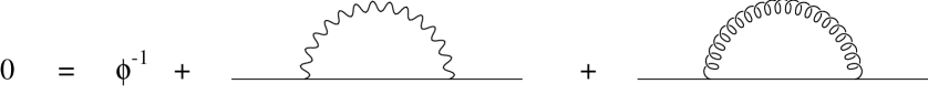
Figure 2: Schwinger Dyson equation for $\phi$ field at $O(1/N)$.

To solve for $\omega_{1}$ one substitutes the asymptotic scaling values into the lines of the Schwinger Dyson equations of each of the fields. These are illustrated in Figures $2$ and $3$. In the latter we have only indicated the possible topologies that arise due to the nature of the expansion in powers of $1/N$ and each wiggly line represents all possible combinations of $\sigma$ and $T^{ab}$ fields. If we ignore for the moment the two and three loop corrections in Figure $3$ we find the equations are represented by

$$0 = p(\alpha)\left[1~{}-~{}q(\alpha,\omega)(x^{2})^{\omega}A^{\prime}\right]~{}+~{}z\left[1~{}+~{}\left(A^{\prime}+B^{\prime}\right)(x^{2})^{\omega}\right]$$

$$+~{}\frac{(m-1)(m+2)y}{2m}\left[1~{}+~{}\left(A^{\prime}+C^{\prime}\right)(x^{2})^{\omega}\right]$$

$$0 = p(\beta)\left[1~{}-~{}q(\beta,\omega)(x^{2})^{\omega}B^{\prime}\right]~{}+~{}\frac{1}{2}Nmz\left[1~{}+~{}2(x^{2})^{\omega}A^{\prime}\right]$$

$$0 = p(\gamma)\left[1~{}-~{}q(\gamma,\omega)(x^{2})^{\omega}C^{\prime}\right]~{}+~{}\frac{1}{2}Ny\left[1~{}+~{}2(x^{2})^{\omega}A^{\prime}\right]$$ (3.14)

at the CS fixed point which we consider first for illustration. These equations decouple on dimensional grounds into a set which determine $\eta$ at CS and a set involving $\omega$. The former lead to the values for $\eta_{1}$, $z_{1}$ and $y_{1}$ quoted above. For the latter set of equations for consistency the determinant of the $3$ $\times$ $3$ matrix defined with respect to the basis vector $\{A^{\prime},B^{\prime},C^{\prime}\}$ has to vanish which naively leads to the equation

$$0~{}=~{}\frac{(m-1)(m+2)}{m}yq(\beta,\omega)~{}-~{}q(\gamma,\omega)\left[2z~{}-~{}(1+q(\alpha,\omega))q(\beta,\omega)\left[z~{}+~{}\frac{(m-1)(m+2)}{2m}y\right]\right]\,.$$ (3.15)

This is similar to the consistency equation which determines the exponent denoted by $\lambda$ in [23, 24] where the correction to scaling exponent has canonical dimension $\lambda_{0}$ $=$ $\mu$ $-$ $1$. However, for this value $q(\alpha,\lambda_{0})$ with $\alpha$ $=$ $(\mu$ $-$ $1)$ or $2$ canonically is always an $O(1)$ quantity. By contrast, for the four dimensional model $q(\alpha,\omega_{0})$ with $\omega_{0}$ $=$ $(\mu$ $-$ $2)$ and $\alpha$ $=$ $(\mu$ $-$ $1)$ or $2$ it has values which are $O(N)$ and $O(1/N)$ respectively and therefore affects the consistency equation. For instance, whilst the product $q(\alpha,\omega)q(\beta,\omega)q(\gamma,\omega)$ in (3.15) will be $O(1/N)$, this equation, (3.15), would give an incorrect value for the exponents since the contributions in (3.15) from $\sigma^{-1}$ and $\sigma_{T}^{-1}$ are of the same order in $1/N$ as those from the two and three loop correction graphs of Figure $3$ which we had naively omitted. Thus to determine $\omega_{1}$ correctly one must include the contributions from these diagrams to the $B^{\prime}$ and $C^{\prime}$ parts of the Schwinger Dyson representation in the asymptotic approach to the fixed points. Hence, the $\sigma$ and $T^{ab}$ equations in (3.14) are modified to

$$0 = p(\beta)\left[1~{}-~{}q(\beta,\omega)(x^{2})^{\omega}B^{\prime}\right]~{}+~{}\frac{1}{2}Nmz\left[1~{}+~{}2(x^{2})^{\omega}A^{\prime}\right]$$

$$+~{}\left[\frac{1}{2}Nmz^{2}\Pi_{1}B^{\prime}~{}+~{}\frac{1}{4}(m+2)(m-1)Nyz\Pi_{1}C^{\prime}\right.$$

$$\left.~{}~{}~{}~{}+~{}N^{2}m^{2}z^{3}\Pi_{2}B^{\prime}~{}+~{}\frac{1}{2}(m+2)(m-1)N^{2}y^{2}z\Pi_{2}C^{\prime}\right](x^{2})^{\omega}$$

$$0 = p(\gamma)\left[1~{}-~{}q(\gamma,\omega)(x^{2})^{\omega}C^{\prime}\right]~{}+~{}\frac{1}{2}Ny\left[1~{}+~{}2(x^{2})^{\omega}A^{\prime}\right]$$ (3.16)

$$+~{}\left[\frac{1}{2}Nyz\Pi_{1}B^{\prime}~{}+~{}\frac{(m-2)}{4m}Ny^{2}\Pi_{1}C^{\prime}~{}+~{}N^{2}y^{2}z\Pi_{2}B^{\prime}\right.$$

$$\left.~{}~{}~{}~{}+~{}N^{2}y^{2}z\Pi_{2}C^{\prime}~{}+~{}\frac{(m-2)(m+4)}{4m}N^{2}y^{3}\Pi_{2}C^{\prime}\right](x^{2})^{\omega}~{}.$$

In these equations to ensure the correct contribution to the $\omega$ Schwinger Dyson equation after decoupling one correction term, $(x^{2})^{\omega}$, is on one internal $\sigma$ or $T^{ab}$ line. There are corrections to the $\phi$ lines but these only contribute to $\omega_{2}$ after examining where they appear in the consistency determinant. This feature of having to include higher order graphs to obtain the correct $\omega_{1}$ is not peculiar to the CS fixed point as it already occurs at the Heisenberg point, [26]. With these additional diagrams the correct consistency equation is given by setting the determinant of the matrix

$$\left[\begin{array}[]{ccc}(1+q(\alpha,\omega))\left[z+\frac{(m-1)(m+2)}{2m}y\right]&z&\frac{(m-1)(m+2)}{2m}y\\ 2&q(\beta,\omega)+z\Pi_{1}+2mNz^{2}\Pi_{2}&\frac{(m-1)(m+2)}{2m}y(\Pi_{1}+2Ny\Pi_{2})\\ 2&z(\Pi_{1}+2Ny\Pi_{2})&\left[q(\gamma,\omega)+\frac{(m-2)(m+4)}{2m}Ny^{2}\Pi_{2}\!\!\right.\\ &&\left.+\frac{(m-2)}{2m}y\Pi_{1}+2Nyz\Pi_{2}\right]\\ \end{array}\right]$$ (3.17)

to zero.

Figure 3: Basic topologies for the corrections to the $\sigma$ and $T^{ab}$ Schwinger Dyson equations to determine $\omega$ at $O(1/N)$.

Therefore, to solve for the respective $\omega$’s from (3.17) the values of these additional diagrams must be computed. As the graphs are similar to those used in the $O(N)$ $\phi^{4}$ calculation of $\omega$ if the group theory of each graph is suppressed we merely quote the $d$-dimensional values for the respective two and three loop graphs of Figure $3$. They are, ignoring symmetry factors,

$$\Pi_{1}~{}=~{}[\nu(2,\mu-1,\mu-1)]^{2}~{}~{}~{},~{}~{}~{}\Pi_{2}~{}=~{}[\nu(2,\mu-1,\mu-1)]^{2}\nu(1,2,2\mu-3)\nu(4-\mu,\mu-1,2\mu-3)$$ (3.18)

where $\nu(x,y,z)$ $=$ $a(x)a(y)a(z)$. These were calculated using the method of uniqueness of [28] which was extended from three dimensions to $d$-dimensions in [23, 24]. Futher, since the $O(1/N)$ values of $q(\beta,\omega)$ and $q(\gamma,\omega)$ now need to be included it transpires that the $O(1/N)$ expression for the vertex anomalous dimensions, $\chi$ and $\chi_{T}$, are required. This is due to

$$q(\beta,\omega)~{}=~{}\frac{a(4-\mu)\Gamma(\mu)}{a(2)a(2-\mu)}\frac{[\omega_{1}-\eta_{1}-\chi_{1}]}{N}~{}+~{}O\left(\frac{1}{N^{2}}\right)~{}.$$ (3.19)

We have computed each vertex anomalous dimension at each fixed point and find

$$\chi^{\mbox{\footnotesize{CS}}}_{1} = -~{}\frac{\mu(4\mu-5)\eta^{\mbox{\footnotesize{CS}}}_{1}}{(\mu-2)}$$

$$\chi^{\mbox{\footnotesize{CS}}}_{T,1} = -~{}\frac{\mu[(2\mu-3)m+(4\mu-5)]\eta^{\mbox{\footnotesize{CS}}}_{1}}{(\mu-2)(m+1)}$$

$$\chi^{\mbox{\footnotesize{AU}}}_{T,1} = -~{}\frac{\mu(m-2)[(m+4)(2\mu-3)+1]\eta^{\mbox{\footnotesize{AU}}}_{1}}{(m-1)(m+2)(\mu-2)}~{}.$$ (3.20)

The expression for $\chi^{\mbox{\footnotesize{CS}}}_{1}$ is formally the same as that for the $O(1/N)$ vertex dimension at the Heisenberg fixed point. For each exponent we have computed the value by applying the technique of [29] of large $N$ critical point renormalization of $3$-point functions to each vertex at the appropriate fixed point. For $\chi$ we have checked that the value agrees with that given by the scaling law which emerges from the theory which is in the same universality class as (2.2). This is believed to be the $O(N)$ $\times$ $O(m)$ two dimensional nonlinear sigma model where instead of the term quadratic in $\sigma$ of (2.2) one has a term linear in $\sigma$ where its coupling constant is related to the critical exponent $\nu$. However, in such a model it is clear from group theory that there can be no linear term in $T^{ab}$ and therefore both expressions for $\chi_{T}$ cannot be derived from a scaling law but only direct calculation.

With these values we can now determine the solution for the consistency equation for each fixed point. For CS since the matrix is $3$ $\times$ $3$ two values for $\omega$ emerge. These are

$$\omega^{\mbox{\footnotesize{CS}}}_{\pm} = (\mu-2)~{}+~{}\frac{(2\mu-1)\eta^{\mbox{\footnotesize{CS}}}_{1}}{2(m+1)(\mu-2)N}\left[m(\mu-1)(\mu-4)+(2\mu^{2}-7\mu+4)\right.$$

$$\left.~{}~{}~{}~{}~{}~{}\pm~{}\mu\left[(m^{2}-1)(\mu-1)^{2}+2(m-1)(2\mu-3)(\mu-1)+(5\mu-8)^{2}\right]^{\mbox{\small{$\frac{1}{2}$}}}\right]~{}+~{}O\left(\frac{1}{N^{2}}\right)$$

where the $\pm$ subscript refers to the sign in front of the discriminant. Both are perfectly acceptable solutions since one corresponds to one stable direction at CS and the other to the eigenexponent from the second direction.

For AU the derivation of the consistency equation follows the same pattern as that for CS in that two and three loop graphs have also to be included due to the large $N$ counting. The consistency equation itself can be deduced from (3.17) by deleting the second row and column from the matrix and setting $z$ $=$ $0$ in the remaining entries. Since only the $T^{ab}$ field is present only one value for $\omega$ emerges which is

$$\omega^{\mbox{\footnotesize{AU}}}_{+}~{}=~{}(\mu-2)~{}-~{}\left[2\mu^{2}-3\mu-1~{}+~{}\frac{\mu(m-2)[2\mu-5-2(m+4)(2\mu-3)]}{(m-1)(m+2)}\right]\frac{\eta^{\mbox{\footnotesize{AU}}}_{1}}{N}~{}+~{}O\left(\frac{1}{N^{2}}\right)$$ (3.22)

which corresponds to the eigenexponent of the stable direction at AU. For completeness we note that at the Heisenberg fixed point for the stable direction we have, [27, 26],

$$\omega^{\mbox{\footnotesize{Heis}}}_{+}~{}=~{}(\mu-2)~{}-~{}\frac{4(2\mu-1)^{2}\Gamma(2\mu-2)}{\Gamma(2-\mu)\Gamma(\mu-1)\Gamma(\mu-2)\Gamma(\mu+1)mN}~{}+~{}O\left(\frac{1}{N^{2}}\right)$$ (3.23)

which is deduced by deleting the third row and column of (3.17) and setting $y$ $=$ $0$.

In order to check the correctness of each result one can set $d$ $=$ $4$ $-$ $2\epsilon$, or $\mu$ $=$ $2$ $-$ $\epsilon$, and expand each exponent to $O(\epsilon^{3})$ and compare with the values of explicit perturbation theory, (2.11). We find total agreement for all three exponents and therefore regard (LABEL:omlncs) and (3.22) as correct. Indeed equipped with (LABEL:omlncs) and (3.22) we can now reverse the check argument and use the information contained in the $d$-dimensional exponents to determine constraints on the structure of the four loop $\overline{\mbox{MS}}$ corrections to (2.3) and (2.4). First, we record the $\epsilon$ expansion of each of the exponents in the stable directions which are consistent with (2.11). From (LABEL:omlncs), (3.22) and (3.23) we have

$$\omega^{\mbox{\footnotesize{CS}}}_{+,1} = \left[\frac{3(m^{2}+4m+7)}{(m+1)}\epsilon^{2}~{}-~{}\frac{(13m^{4}+72m^{3}+202m^{2}+216m+25)}{2(m+1)^{3}}\epsilon^{3}\right.$$

$$\left.~{}+~{}\frac{(3m^{6}+10m^{5}+21m^{4}-36m^{3}-387m^{2}-326m+395)}{4(m+1)^{5}}\epsilon^{4}~{}+~{}O(\epsilon^{5})\right]$$

$$\omega^{\mbox{\footnotesize{CS}}}_{-,1} = \left[6(m+1)\epsilon~{}-~{}\frac{(13m^{2}+26m+25)}{(m+1)}\epsilon^{2}~{}+~{}\frac{(3m^{4}+12m^{3}+82m^{2}+116m-5)}{2(m+1)^{3}}\epsilon^{3}\right.$$

$$\left.~{}+~{}\frac{[48(m+1)^{6}\zeta(3)+3m^{6}+18m^{5}+29m^{4}+76m^{3}+397m^{2}+322m-397]}{4(m+1)^{5}}\epsilon^{4}\right.$$

$$\left.~{}+~{}O(\epsilon^{5})\right]$$

$$\omega^{\mbox{\footnotesize{AU}}}_{+,1} = \frac{1}{m}\left[(3m^{2}+9m-34)\epsilon^{2}~{}-~{}\frac{1}{2}(13m^{2}+33m-162)\epsilon^{3}~{}+~{}\frac{1}{4}(3m^{2}-5m-54)\epsilon^{4}\right.$$

$$\left.~{}~{}~{}~{}+~{}O(\epsilon^{5})\right]$$

$$\omega^{\mbox{\footnotesize{Heis}}}_{+,1} = \frac{1}{m}\left[18\epsilon^{2}~{}-~{}33\epsilon^{3}~{}-~{}\frac{5}{2}\epsilon^{4}~{}+~{}O(\epsilon^{5})\right]~{}.$$ (3.24)

Next we compare the $O(\epsilon^{4})$ coefficients with those of the explicit perturbative expansion which have been parametrized by $\{a_{i}\}$ and $\{b_{i}\}$. From the Heisenberg exponent we have

$$a_{1}~{}-~{}a_{2}~{}-~{}a_{3}~{}-~{}a_{4}~{}-~{}a_{5}~{}-~{}a_{6}~{}=~{}\frac{5m^{2}}{7776}$$ (3.25)

which agrees with the explicit four loop $\phi^{4}$ computation when one sets $m$ $=$ $1$ and determines the $O(1/N)$ coefficient of the $u^{5}$ term of $\beta_{u}(u,v)$. From the CS fixed point we have

$$2a_{1}~{}+~{}(m-1)b_{2}~{}=~{}-~{}\frac{(3m+7)(m-3)}{15552}$$ (3.26)

and

$$(m+1)[a_{2}~{}+~{}2a_{3}~{}+~{}3a_{4}~{}+~{}4a_{5}~{}+~{}5a_{6}~{}-~{}b_{3}~{}-~{}2b_{4}~{}-~{}3b_{5}~{}-~{}4b_{6}]$$

$$+~{}(2m-1)(m-1)a_{1}~{}-~{}2m(m-2)b_{2}$$

$$=~{}\frac{\zeta(3)}{108(m+1)^{3}}~{}+~{}\frac{(3m^{2}+6m+19)}{5184(m+1)^{5}}~{}.$$ (3.27)

The final constraint arises from the stable direction at the AU fixed point which gives

$$(m-1)^{4}b_{2}~{}+~{}(m-1)^{3}b_{3}~{}+~{}(2m-1)(m-1)^{2}b_{4}~{}+~{}(3m^{2}-3m+1)(m-1)b_{5}$$

$$+~{}(2m-1)(2m^{2}-2m+1)b_{6}$$

$$=~{}-~{}\frac{[3m^{2}-5m-54]}{15552}~{}.$$ (3.28)

One can now deduce the values for the exponents in the four stable directions in three dimensions. These are, with our conventions,

$$\omega^{\mbox{\footnotesize{CS}}}_{+} = -~{}\frac{1}{2}~{}+~{}\frac{4(m+4)}{3\pi^{2}N}~{}+~{}O\left(\frac{1}{N^{2}}\right)$$

$$\omega^{\mbox{\footnotesize{CS}}}_{-} = -~{}\frac{1}{2}~{}+~{}\frac{16(m+1)}{3\pi^{2}N}~{}+~{}O\left(\frac{1}{N^{2}}\right)$$

$$\omega^{\mbox{\footnotesize{AU}}}_{+} = -~{}\frac{1}{2}~{}+~{}\frac{4[m^{2}+4m-8]}{3\pi^{2}mN}~{}+~{}O\left(\frac{1}{N^{2}}\right)$$

$$\omega^{\mbox{\footnotesize{Heis}}}_{+} = -~{}\frac{1}{2}~{}+~{}\frac{32}{3\pi^{2}mN}~{}+~{}O\left(\frac{1}{N^{2}}\right)~{}.$$ (3.29)

For CS the corrections both have the same sign and interestingly neither involves a square root which appears in the $d$-dimensional expression. For the specific case of $m$ $=$ $2$ we have from (3.29)

$$\left.\omega^{\mbox{\footnotesize{CS}}}_{+}\right|_{m=2} = -~{}\frac{1}{2}~{}+~{}\frac{8}{\pi^{2}N}~{}+~{}O\left(\frac{1}{N^{2}}\right)$$

$$\left.\omega^{\mbox{\footnotesize{CS}}}_{-}\right|_{m=2} = -~{}\frac{1}{2}~{}+~{}\frac{16}{\pi^{2}N}~{}+~{}O\left(\frac{1}{N^{2}}\right)$$

$$\left.\omega^{\mbox{\footnotesize{AU}}}_{+}\right|_{m=2} = -~{}\frac{1}{2}~{}+~{}\frac{8}{3\pi^{2}N}~{}+~{}O\left(\frac{1}{N^{2}}\right)$$

$$\left.\omega^{\mbox{\footnotesize{Heis}}}_{+}\right|_{m=2} = -~{}\frac{1}{2}~{}+~{}\frac{16}{3\pi^{2}N}~{}+~{}O\left(\frac{1}{N^{2}}\right)~{}.$$ (3.30)

With these values we can comment on the possible breakdown of stabilty in this model. In our computations so far have relied on the fact that the stability picture for the fixed points represented in Figure 1 is valid for the full range of $N$ in the large $N$ expansion. However, it has been suggested that for certain values of $N$ this scenario may be different and that the underlying assumption of the existence of a second order phase transition, around which the large $N$ critical point formalism is built, could break down. Indeed there is some controversy in this model in three dimensions about the existence of CS and whether the phase transition is first or second order for relatively low values of $N$. Moreover, the precise value of $N$ where the order changes has not been determined consistently from different methods. (A recent review is given in [17].) For instance, a value has been found for this critical value of $N$ by using $d$ $=$ $4$ $-$ $2\epsilon$ dimensional perturbation theory and it was extended to three dimensions using standard resummation techniques, [30], giving $N_{c}$ $=$ $3.39$. By contrast, Monte Carlo methods and another $\epsilon$-expansion extraction have suggested $N_{c}$ $<$ $2$, [6, 7, 8]. With the large $N$ corrections (3.30) we can naively examine the range of values of $N$ for which either CS stability exponent changes sign. For $\left.\omega^{\mbox{\footnotesize{CS}}}_{-}\right|_{m=2}$ this will occur when $N_{c}$ $=$ $3.24$ whilst $\left.\omega^{\mbox{\footnotesize{CS}}}_{+}\right|_{m=2}$ changes sign when $N_{c}$ $=$ $1.62$. The former would suggest a critical $N$ in a similar range to that of [30]. However, these remarks ought to be qualified with various observations. First, we have only computed the $O(1/N)$ correction to stability where $N$ is assumed to be large. Therefore, one has to ask whether the approximation will still be valid for such a low value of $N$. Second, the nature of the large $N$ expansion is a reordering of perturbation theory such that a certain class of diagrams are summed first. Therefore, if one could compute to all orders one would reproduce ordinary perturbation theory and so obtaining a value for $N_{c}$ in three dimensions which is not inconsistent with the resummed value determined from several loop orders in ordinary perturbation theory would seem only to reinforce that particular value. In other words if non-perturbative effects become significant at CS for low values of $N$ to affect the precise location of $N_{c}$ these will have been omitted in perturbation theory. Third, for our value of $N_{c}$ we have naively assumed the large $N$ series is convergent and therefore that our simple assumption that when the $O(1/N)$ correction exceeds $1/2$ the character of the fixed point changes is valid. Only a higher order calculation would resolve this.

4 Discussion.

We have computed the correction to scaling exponents $\omega$ in all the stable directions of the Landau-Ginzburg-Wilson model with $O(N)$ $\times$ $O(m)$ symmetry at $O(1/N)$ in $d$-dimensions. This allows one to extract information in all the available large $N$ exponents of [11] at $O(1/N)$ in relation to the four dimensional theory in the same way that the two dimensional critical slope information contained in the exponent $\nu$ does for the underlying two dimensional theory. It is also worth stressing again, [11], that from the point of view of the large $N$ formalism a consistent picture emerges in terms of the active fields of the theory formulated in terms of the auxiliary fields $\sigma$ and $T^{ab}$ of (2.2). At the Heisenberg and AU fixed points only $\sigma$ and $T^{ab}$ respectively propagate which corresponds in the large $N$ formalism developed here to one stable direction and hence only one eigenexponent emerged. However, at the only fully stable fixed point both fields are relevant leading to two independent stability exponents. This is a natural way to picture this particular model which we assume persists to higher orders in large $N$. Moreover, our consistency with three loop $\overline{\mbox{MS}}$ perturbation theory provides an important internal cross check on the values of quantities, such as the vertex anomalous dimensions, which we had to compute en route to our expressions for $\omega_{i}$. Further, the information contained within the expressions (LABEL:omlncs), (3.22) and (3.23) will provide important checks on any future explicit four loop $\overline{\mbox{MS}}$ perturbative calculations which would improve the accuracy of the numerical estimates deduced from (2.3), (2.4) and other renormalization group functions. Such four loop calculations are certainly viable since five loop results are available in $\overline{\mbox{MS}}$ in ordinary $O(N)$ $\phi^{4}$ theory. For example, the integration routines for the four loop Feynman diagrams have already been constructed. However, one can also attack this problem from the large $N$ point of view. For instance, we have demonstrated the elegance of the formalism to produce the critical eigenexponents at $O(1/N)$. However, this machinery has already been extended in [26] to compute $\omega_{2}$ in the Heisenberg model. Therefore, we would expect there to be no serious obstacles to extending the present computation to find $\omega^{\mbox{\footnotesize{CS}}}_{2}$ and $\omega^{\mbox{\footnotesize{AU}}}_{2}$. For example, the values of the underlying three, four, five and six loop Feynman diagrams which are analogous to the corrections of Figure $3$ for the $O(1/N^{2})$ calculation have been determined. We hope to return to this in a future article.