Static Axisymmetric Vacuum Solutions and Non-Uniform Black Strings

Abstract

We describe new numerical methods to solve the static axisymmetric vacuum Einstein equations in more than four dimensions. As an illustration, we study the compactified non-uniform black string phase connected to the uniform strings at the Gregory-Laflamme critical point. We compute solutions with a ratio of maximum to minimum horizon radius up to nine. For a fixed compactification radius, the mass of these solutions is larger than the mass of the classically unstable uniform strings. Thus they cannot be the end state of the instability.

1 Introduction

Static axisymmetric vacuum gravity in four dimensions is generally solved by the elegant Weyl solutions [1] which reduce the 3 independent Einstein equations to one elliptic Laplace equation. However, solutions other than Schwarzschild and flat space are nakedly singular, or contain conical deficits. In $d$ dimensions higher than four, one can consider static axisymmetric solutions with a rotational $O(d-2)$ spatial isometry group. Then there are a far richer variety of solutions, notably including the black strings, which evade such problems. However no general analytic solution is known for more than four dimensions [2, 3].

Interest in black strings was aroused when Gregory and Laflamme [4, 5, 6] showed that the uniform black string, a simple product of a Schwarzschild solution with a line, is unstable to modes with wavelength larger than a critical value. Using entropy arguments they concluded that the end state of the classical instability would be a sequence of black holes. The critical deformation mode is static, and led Gregory and Laflamme to point out the existence of a new family of black string solutions without translational invariance, the non-uniform strings.

Compactifying the line direction to a circle allows uniform black strings to be stabilised for values of the circle radius smaller than the critical instability length. In the following, when we refer to a string we implicitly mean a compactified one unless otherwise stated. Such string solutions are important in understanding the process of black hole formation in extra dimensions, both in Kaluza-Klein theory and more generally in the presence of branes [7, 8], and their classical stability has also been considered in AdS [9, 10, 11, 12].

Gubser and Mitra used AdS-CFT arguments to conjecture that the onset of the classical instability of uniform strings coincides with local thermodynamic instability [13, 14], and their work has subsequently been generalised [15]. This was later proved using Euclidean methods by Reall [16], the translational invariance playing a crucial role, and further considered in [17]. The dynamics of the uniform black string classical instability, and its subsequent decay to black holes was questioned by Horowitz and Maeda [18] who showed that the horizon could not pinch off in a finite affine time. They then argued that the end state might instead be a non-uniform string. Gregory and Laflamme had constructed the non-uniform strings to linear order in perturbation theory. In order to understand the properties of these solutions, Gubser [19] went to higher order in the marginal deformation, and showed that the mass of these non-uniform solutions increases from that of the critical string, for the same circle length.

In light of Horowitz and Maeda’s result, Gubser suggested that at finite deformation the mass of the non-uniform strings would decrease below that of the critical string mass, and their entropy would be larger than a uniform string of the same mass, and circle length, therefore allowing a non-uniform string to be the end state of the critical string instability. This indicated the transition from uniform to non-uniform string would be first order, and thus non-adiabatic. It is important to note that the Horowitz-Maeda result does not remove the possibility of a black hole end state. This could involve infinite affine time, with possibly complicated dynamics associated with the horizon pinching, although they give arguments why this would be unlikely. Alternatively the dynamics could be more complicated, and evade the assumptions of the Horowitz and Maeda proof. For example, naked singularities might be present in the intermediate stages, signalling a dynamic violation of cosmic censorship, as originally postulated by Gregory and Laflamme [4]. Indeed the end state may even be nakedly singular itself.

Further evidence supporting the first order nature of the transition was reported in [20] where unpublished numerical work by Choptuik et al [21] is said not to have found smooth evolution to a non-uniform phase. However they cannot yet determine the end state. Note that there is no known generally stable algorithm for numerical evolution of general relativity [22] and therefore studying an unstable system for long dynamical times is an extremely difficult problem.

Analytically finding these solutions for finite deformation would allow the issue of their classical stability and thermodynamic properties to be settled. A very interesting analytic attempt was made by Harmark and Obers [23] where the usual 3 degrees of freedom in the axisymmetric metric were reduced to only one using a conjectured ansatz. It seems difficult to show whether this is indeed a consistent ansatz, and at first sight it appears very optimistic. What lends considerable weight to their conjecture is that they have shown that it is consistent to second order in an asymptotic expansion, which is a highly non-trivial result. Unfortunately, the resulting equation for the unknown is very complicated, and indicates, should the ansatz be consistent, that there is little hope in having a convenient integrable form. Using some assumptions, they claim their ansatz indicates new neutral non-uniform solutions exist, which are distinct from those emerging from the uniform strings via the Gregory-Laflamme marginal modes. This remains to be shown, but would naturally be extremely interesting if it were confirmed. The existence of charged near extremal solutions was also considered by Horowitz and Maeda who have shown that non-uniform solutions exist [24] by considering initial data. The classification of the compactified black hole metric was considered in [25].

In a recent paper Kol considered the black string/hole phase diagram. He argues that a classically stable non-uniform phase is too difficult to include in the phase diagram and therefore probably does not exist. However it must be noted that, amongst other assumptions, the work uses thermodynamics to understand the classical stability. The relation between the two has been shown in the case of strings with a non-compact translational symmetry [13, 14, 16]. To date, there is no known relation between classical and local thermodynamic stability for cases without this translation symmetry, such as the non-uniform strings. Kol conjectures that the mass of the non-uniform phase is always greater than that of the critical string, and furthermore the family of solutions is continuous through a topology changing point where non-uniform strings become black holes.

In this paper we hope to resolve the thermodynamic properties of the non-uniform string solutions. The methods we use will be numerical, and follow from techniques developed in [26] to study the geometry of stars on a UV Randall-Sundrum brane [27, 28]. There we observed that a particular gauge made the second derivatives appearing in a subset of the Einstein equations appear elliptic, in line with our expectation that the static equations should indeed be elliptic. We showed how to employ elementary numerical methods to solve these equations, and in addition how to implement the constraints on the boundary data, and to ensure they are globally satisfied.

In section 2, we begin by briefly reviewing this method in a more general context, and then in section 3, show how to apply it to the black string in 6 dimensions. Note that we study the 6 dimensional string for various simplifying technical reasons, although the previous results in the literature all apply equivalently in the 5 and 6 dimensional cases. In particular, repetition of Gubser’s work in the 6 dimensional case again yields the same conclusion, that a non-uniform string emerging from the critical point has larger mass than the critical string, and lower entropy than a uniform string of the same mass. Thus the transition from the unstable uniform string to whatever end state it eventually reaches is again non-adiabatic, as there is no other family of connected solutions.

The compactified black strings provide a clean application for our numerical method, where it is very simple to implement. This is compared to the previous work of the star on the UV brane [26], where various technical issues associated with the coordinate system at the symmetry axis complicated matters. The method, based on elementary relaxation techniques, yields solutions with large deformation parameter. The implementation of the method will be made available at [29]. The performance of the method is evaluated in section 4, and self-consistency is demonstrated. Using moderate resolution and computing time we present solutions with a maximum/minimum horizon radius of around ten. This can no doubt be considerably improved by further development of the algorithm and relaxation methods. Due to the technical nature of this section, the reader might wish to pass over this directly to the following section 5, where the solutions and their properties are discussed. These solutions allow us to see the prevailing asymptotic behaviour for fixed circle length, namely that the mass, which increases with increasing non-uniformity near the critical solution as shown by Gubser, continues to increase until it appears to reach an asymptotic value of approximately twice that of the critical string, for maximally non-uniform string solutions. Several independent consistency checks are performed to estimate the systematic errors present in the method, and we find that they are small, and thus this mass result is expected to be robust. In addition we compute the difference of the entropy of the non-uniform strings to uniform ones of the same mass, finding that the non-uniform solutions always have the lower entropy. However, this entropy difference is very small, and thus is ‘difficult’ to measure numerically using the current implementation, and so we consider this result less concrete.

Although we are using relaxation methods, we do not have an energy functional to minimise. Therefore whilst we find the non-uniform solutions, we cannot infer their classical stability. It is, however, intriguing that when applying the method to find uniform string solutions, only the classically stable solutions can be found by our method.

In section 6, we discuss the implications, that the non-uniform static solutions do indeed exist non-perturbatively, but are not accessible as the decay product of a classically unstable uniform black string due to their higher mass. If they are classically stable, their behaviour is presumably similar to uniform strings with greater than critical mass, namely that they quantum mechanically radiate until the critical point is reached, and then classically decay. They would possibly play an important role in higher dimensional dynamics, particularly in black hole formation with compactified extra dimensions, where the black hole mass is in the range where both the uniform and non-uniform solutions exist. If they are classically unstable, as conjectured by Kol, then the solutions would classically decay, and are likely to play little role in higher dimensional dynamics. Starting with a solution, we have shown that the decay to the uniform strings with the same, or slightly lower mass is allowed by the second law, although the mass difference cannot be very large, as the difference in horizon volume, or entropy, between the non-uniform and uniform strings of the same mass is always small. This possibility is then quite the opposite of the Horowitz and Maeda picture. Here the non-uniform solutions might decay to the uniform stable solutions. Alternatively, if much radiation is given off in the decay, it is likely that the non-uniform strings will behave in much the same way as the unstable uniform strings. These different behaviours are summarised in figure 1. Whichever case is true, the fascinating question of the end state of the GL instability remains open, as members of this branch of non-uniform solutions cannot be the end state. Following the Horowitz-Maeda result, this may signal the existence of new non-uniform solutions unconnected to the GL critical point, or alternatively, novel decay dynamics, possibly involving cosmic censorship violation.

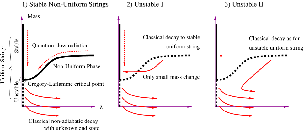
Figure 1: Summary of results: We have shown by numerical methods that the non-uniform branch of solutions always has larger mass, for a fixed compactification radius, than the critical uniform string. This implies that the non-uniform strings cannot be the end state of the Gregory-Laflamme instability for the unstable uniform strings. Not knowing the classical stability of these non-uniform solutions there are 3 plausible scenarios. 1) The non-uniform strings are classically stable, and may quantum mechanically decay by Hawking radiation to the critical point, like uniform stable strings. 2) They are classically unstable and decay to stable uniform strings. We have shown the horizon volume, or entropy, of non-uniform strings is always less than that of a uniform string of the same mass, so this is allowed by the second law, although the mass lost in the decay must be small. 3) They are classically unstable and decay in the same way as the unstable uniform strings. If stable, it is likely these solutions may play an important role in black hole formation in compactified theories.

2 Static Axisymmetric Gravity with Elliptic Boundary Conditions

The problem that concerns us is solving static vacuum gravity. This is thought to be elliptic (ie. a boundary value problem) in the sense that it is consistent with imposing data, say the induced metric, on all coordinate patch boundaries. In referring to boundaries we mean to include asymptotic boundaries. The simplest example where the Einstein equations are manifestly elliptic is in the Newtonian limit of gravity. There we see that the Newtonian potential obeys a Laplace equation, or Poisson equation in the presence of matter. Of course this is only a perturbative description, but is strongly suggestive that for small deformations of the boundary data away from a non-linear solution, we might use elliptic methods.

Conventional numerical gravity problems are dynamical, where initial data on some Cauchy surface is given, and the equations are then evolved hyperbolically off that surface [22]. It is true that elliptic equations may be solved in a ‘hyperbolic’ fashion, if data can be consistently imposed on a subset of the boundaries. However, if the problem specifies data on all the boundaries, as is often physically the case, then such methods will result in shooting problems. Whilst shooting is acceptable for an ordinary differential equation, it is no longer a good method for solving a 2 variable partial differential equation. In such a case, solutions are best obtained by relaxation, or in linear cases, by spectral methods. The key question we begin to answer is how to implement a relaxation scheme for gravity. The methods we outline in this paper are tailored to the axisymmetric case, as we are primarily interested in exploring the properties of the black string in higher dimensions. However, generalisations of these methods may well apply in situations with different, or even less symmetry.

In 4 dimensions the elegant Weyl solutions [1] provide a non-linear general solution to the axisymmetric problem. The solution reduces to solving a scalar Laplace equation in flat 3 dimensional space for axisymmetric solutions, and thus we see the elliptic nature of the static problem. Most vacuum Weyl solutions have some form of naked curvature or angular deficit singularity, and there is no asymptotically flat black string solution. In higher dimensions, where axisymmetric solutions may be asymptotically flat in the radial direction, with no naked singularities, such as for the 5 dimensional black string, there is no known general analytic solution. Whilst the Weyl solution does generalise to higher dimensions [30, 2, 3], it does not describe axisymmetric geometries. Finding this general axisymmetric solution is an important open problem. In 4 dimensions the radial sub-manifold is an $S^{1}$ and is therefore flat. However this is no longer true in higher dimensions, which considerably complicates the form of the Einstein equations. Indeed there is no reason to expect these to be integrable, and there to exist a closed form general solution.

The methods used in this paper were first applied in [26] to solve the geometry of a star on a Randall-Sundrum brane near its upper mass limit. This enabled the geometry of stars with radius smaller than the AdS length to be found, and in addition, we confirmed that effective 4 dimensional gravity is reproduced in the non-linear regime for large stars. These are the only calculations for strongly gravitating small sources on branes where the bulk is consistently solved for, except special cases [31, 32], where the Weyl, or generalised Weyl solutions [2] can be applied. For numerical work on brane black holes, based on shooting methods, see [33], where the difficulty of shooting with partial differential equations is apparent. However, generic behaviour of the bulk geometry near the brane can be studied for some initial guess on the brane, although it appears to be pathological far from the brane, as one would expect from shooting. A more recent similar work is [34]. Note that for strongly gravitating large objects, analytic progress can be made when the extra dimension is compact [35, 36]. However these derivative expansion methods cannot be applied for the black strings considered here, as the change in curvature radius due to the non-uniformity is large compared to the compactification radius.

In some respects the case of the black string is technically simpler to implement than the Randall-Sundrum star, and thus provides an archetypal example of our method. In the rest of the section we review the general features of the axisymmetric relaxation method, and in the following section we explicitly show how to apply it to the black string.

2.1 A Relaxation Method for Solving Static Gravity

Having resorted to a numerical solution we must ask why solving an elliptic axisymmetric problem is difficult. In a scalar field theory context, finding numerical solutions to the elliptic static equations of motion is essentially trivial, simply a matter of using standard relaxation techniques on the Hamiltonian. One difficulty for gravity is that there is no local energy functional that is positive definite in the metric and its derivatives. Therefore standard relaxation techniques cannot be applied. More difficult still is the presence of constraints in the Einstein equations. Let us consider axisymmetry and use coordinate freedom to locally parametrise our metric with the minimal number of functions generally compatible with this symmetry. There are then 3 metric functions required, but 5 Einstein equations. One crucial feature of our technique will be to choose a coordinate system such that 3 of these 5 Einstein equations appear to be elliptic, with their second derivative terms having a Laplace form. We call these equations the ‘interior equations’. Let us then simply assume that, although there is no energy function to minimise, we may successfully solve these equations for the boundary data given. However, how can we guarantee this solution also satisfies the 2 remaining Einstein equations, which we term the ‘constraints’?

In a hyperbolic ADM evolution [37] the constraint equations must only be imposed on the initial surface and then, in an ideal evolution, can be ignored as the Bianchi identities ensure that they remain satisfied. The constraint equations involve the induced metric on the Cauchy surface and its normal derivative, the extrinsic curvature. For a hyperbolic evolution this is exactly what must be specified, the data and its normal time derivative, and thus the constraints may be evaluated.

In our elliptic problem we envisage giving one piece of data on all boundaries, such as the induced metric, rather than all the data, the metric and normal derivative. Now we cannot evaluate the constraints at the boundaries simply based on the data we specify. Knowing the induced metric, we will not know the normal derivatives entering the constraints until we have solved the interior equations. Thus in a hyperbolic evolution, ensuring the constraints are satisfied and evolving the remaining interior equations are separable processes. For the elliptic case, we cannot evaluate the constraints until we have solved the interior equations. Thus we must impose the constraints in an iterative manner, initially picking some boundary data, solving the interior equations, evaluating the constraints and then modifying the boundary data to hopefully improve the constraints on the boundaries, and therefore in the interior. This is repeated until the desired result is obtained. In addition, we must ensure that satisfying the constraints on the boundaries does indeed imply they are satisfied in the interior.

Thus naively we update 2 constraints on the boundaries, specifying 3 metric functions there. Unlike the case of field theory however, the position of the boundaries may well be additional data, as the metric solution defines the geometry of the space itself. If a general coordinate transformation that moves the boundaries does not preserve the form of the metric, then extra degrees of freedom must be used to parameterise the position of these boundaries. In addition to the 2 constraint equations, one must also iteratively update this boundary position. In this general case we may count local data; (1 function for the boundary position) + (3 metric functions) - (2 constraints) = (2 remaining functions), providing the physical data.

Let us now be more explicit and outline a gauge choice that simplifies the above procedure considerably and ensures that the interior equations do have an elliptic form.

2.2 The ‘Conformal Gauge’

Let us take the static axisymmetric metric to depend on a radial variable $r$, and a cylindrical variable $z$. Following [26], we choose a metric that has invariance under conformal transformations in the $r,z$ plane, namely,

$$ds^{2}=g_{\mu\nu}(r,z)dx^{\mu}dx^{\nu}=-e^{2A}dt^{2}+e^{2B}(dr^{2}+dz^{2})+e^{2C}d\Omega^{2}_{d-3}$$ (1)

where $A,B,C$ are functions of $r,z$, and the line element $d\Omega^{2}_{d-3}$ is that of a unit $(d-3)$-sphere. We may always use the $r,z$ coordinate degrees of freedom to locally choose a metric of this form, therefore reducing the 5 possible metric functions of the most general metric to only 3. We note this is reminiscent of the diagonal Weyl form of the metric in 4 dimensions.

We find 3 ‘interior’ Einstein equations from $G^{t}_{~{}t}$, $G^{\theta}_{~{}\theta}$, and $(G^{r}_{~{}r}+G^{z}_{~{}z})$, where $\theta$ is an angle on the $(d-3)$-sphere, which yield equations for $X_{i}=\{A,B,C\}$ of the form;

$$\nabla^{2}X_{i}=\mathrm{src}_{X_{i}}$$ (2)

where $\nabla^{2}=\partial_{r}^{2}+\partial_{z}^{2}$, and the sources $\mathrm{src}_{X_{i}}$ depend non-linearly on all the $X_{j}$, $\partial_{r}X_{j}$ and $\partial_{z}X_{j}$. The diagonal form of the metric ensures that no mixed second derivatives appear in these equations. The conformal invariance in $r,z$ results in the simple Laplace form for the second derivatives.

As in [26], we suppose that in general, an iterative scheme may be implemented to solve these interior equations for $A,B,C$ for some boundary data ‘near’ to that of a known reference solution $\tilde{A},\tilde{B},\tilde{C}$. Whilst there is no energy functional, we may implement a simple Gauss-Seidel scheme [38], treating the sources as fixed. Given a starting ‘guess’ for $A,B,C$, usually chosen to be the known solution, so that initially $X_{i}=\tilde{X}_{i}$, the source terms are calculated and the resulting Poisson equations are then solved for the boundary data, keeping these sources fixed. This gives rise to a new $A,B,C$. The sources are updated with these new values and the process is iterated. Whilst there is certainly no guarantee of convergence, and much freedom in implementation of the iterative scheme, we have found in [26] and in case of the black string presented here, convergence is achieved using the simplest implementations. Thus whilst these interior equations are extremely difficult to study analytically, numerically they are in fact rather easy.

Now we consider the two remaining equations, the ‘constraints’, $G^{r}_{~{}z}$ and $(G^{r}_{~{}r}-G^{z}_{~{}z})$, whose second derivative structure is not of Laplace form. Instead $G^{r}_{~{}z}$ contains only mixed second derivatives of the form $\partial_{r}\partial_{z}X_{i}$ and $(G^{r}_{~{}r}-G^{z}_{~{}z})$ contains only hyperbolic second derivatives as $(\partial_{r}^{2}-\partial_{z}^{2})X_{i}$. These equations are related to the interior ones by the Bianchi identities.

The ‘conformal gauge’ has ensured we have interior equations with Laplace second derivatives as we had hoped for. The next crucial feature of this gauge is that we have residual coordinate freedom to move the boundaries in the $r,z$ plane. These may then be placed anywhere, and choosing the boundary locations completely fixes the residual coordinate freedom. We might contrast this with a metric choice of the form $ds^{2}=-e^{2A}dt^{2}+e^{2B}dr^{2}+e^{2C}r^{2}d\Omega^{2}+dz^{2}$, where such a coordinate transformation does not preserve the form of the metric.

We might be confused that losing the one function parameterising the coordinate position of the boundary would ruin the counting of degrees of freedom given above. Now (3 boundary metric functions) - (2 constraints) seems to only yield one physical degree of freedom? The second feature of the gauge is that only one of the constraint equations must actually be satisfied on all boundaries, and then the second automatically is too, provided it is enforced at just one point. The key is the Bianchi identities. Assuming the interior equations are satisfied, having been relaxed as discussed above, the remaining terms in the Bianchi identities give simple Cauchy-Riemann relations,

$$\partial_{r}\left(g\,G^{r}_{~{}z}\right)+\partial_{z}\left(\frac{g}{2}\,(G^{r}_{~{}r}-G^{z}_{~{}z})\right) =0$$

$$\partial_{z}\left(g\,G^{r}_{~{}z}\right)-\partial_{r}\left(\frac{g}{2}\,(G^{r}_{~{}r}-G^{z}_{~{}z})\right) =0$$ (3)

where $g=\det{g_{\mu\nu}}$. This elegant result implies both constraints, multiplied by the volume element, separately satisfy Laplace equations. Thus if one of them is zero on all boundaries, it must be zero over the whole interior. Furthermore, the Bianchi identities then imply the other is determined to be a constant. Therefore, consider that we implement a scheme which ensures that the $G^{r}_{~{}z}$ constraint is satisfied on all boundaries, so $G^{r}_{~{}z}$ is uniquely determined to be zero in the interior. Then $(G^{r}_{~{}r}-G^{z}_{~{}z})$ must only be imposed at a single point to ensure that it is also true in the interior. Again, this is the unique solution.

We immediately see the power of the conformal gauge over other choices. Not only do we not have to include and relax extra degrees of freedom to parametrise the boundary positions, we also only have to ensure one constraint is satisfied on all the boundaries. We only need satisfy the other constraint at a single point. In addition, it guarantees Laplace like second derivatives for the interior equations. Taken together, these features hugely simplify the task of implementing an algorithm.

It is numerically sensible to redefine $A,B,C$, by subtracting off $\tilde{A},\tilde{B},\tilde{C}$ so that when these functions are zero, the metric is then the reference non-linear solution. Thus in [26], the redefinition introduced a warp and radial scale factor to give AdS in axisymmetric coordinates when $A,B,C$ vanished. The philosophy is to then consider deformations about this non-linear solution. The linear theory is manifestly elliptic, and gives much information regarding the correct boundary conditions to impose. Thus we expect convergence for small perturbations. However, the method will generically allow one to go beyond small deformations.

3 A Prototype Example: Vacuum Black Strings

We now discuss the application of the ideas outlined above, to the construction of compactified non-uniform neutral black strings, in the branch of solutions connected to the GL critical point. The implementation of the numerical method developed here will be made available at [29]. The problem of finding these solutions on an $S^{1}$ is a prototype elliptic one. Asymptotically the geometry is a product of flat space with the $S^{1}$, horizon boundary conditions with some degree of ‘wiggliness’ must be imposed in the interior, and periodicity must be imposed along the $S^{1}$ direction. The scale invariance of the vacuum Einstein equations means that finding the solutions for a fixed $S^{1}$ size allows all other solutions to be generated simply by a scaling. In a dynamical context we can take the length of the asymptotic $S^{1}$ to be fixed, and thus we will be imposing boundary conditions so that string solutions with different uniformity are generated having the same asymptotic $S^{1}$ radius.

In fact we will consider the 6 dimensional black string solution, rather than the 5 dimensional one examined by Gubser. It must be stressed that the Horowitz-Maeda result is dimension independent, and we repeat Gubser’s analysis in Appendix A, finding exactly the same thermodynamic character. Thus the physical behaviour of the GL instability appears to be the same in both 5 and 6 dimensions. The reasons for considering the 6 dimensional string are twofold. Firstly, the black string metric takes a particularly simple form in the conformal gauge in 6 dimensions,

$$ds^{2}=-\frac{r^{2}}{m+r^{2}}e^{2A}dt^{2}+e^{2B}(dr^{2}+dz^{2})+e^{2C}(m+r^{2})d\Omega^{2}_{3}$$ (4)

where $z$ is now an interval as the string is wrapping an $S^{1}$. In contrast to this elegant form, the 5-dimensional conformal gauge metric is far less convenient. The second reason is that the metric perturbation dies away faster, the higher the dimension. In 5 dimensions $C\sim\ln r/r$ whereas in 6 dimensions $C\sim 1/r$. As the lattice must be cut off at a finite $r$ for practical calculations, we expect to get better accuracy for the faster fall off.

When we deform the geometry from the uniform black string we will wish to characterise the geometric deformation. Following Gubser we will use the quantity,

$$\lambda=\frac{1}{2}\left(\frac{\mathcal{R}_{max}}{\mathcal{R}_{min}}-1\right)$$ (5)

where $\mathcal{R}_{max}$ is the maximum radius of the 3-sphere at the horizon and $\mathcal{R}_{min}$ is the minimum. Thus $\lambda$ is zero for the homogeneous black string. We will consider other geometric quantities to be functions of $\lambda$, and we take $\lambda$ to parameterise the path of non-uniform solutions. Thermodynamic quantities of interest will be the horizon temperature, the horizon volume and thus entropy of the string, and the mass. In Appendix A we describe Gubser’s perturbation method applied to the 6 dimensional string in conformal gauge. Using this construction we gain valuable information about the asymptotic behaviour of the metric. It also allows us to test how well our non-linear method performs by directly comparing solutions for small $\lambda$. In addition we can see the range of validity of the perturbation results when $\lambda$ becomes of order unity.

Gubser’s method generates a finite set of ordinary differential equations at each order in the expansion, and these are solved using shooting methods. This is achieved by decomposing the metric functions into Fourier components as,

$$X_{i}(r,z) =\Sigma_{n=0}^{\infty}\bar{\lambda}^{n}X^{n}_{i}(r)\cos(nKz)$$

$$X^{n}_{i}(r) =X^{n(0)}_{i}(r)+\bar{\lambda}^{2}X^{n(1)}_{i}(r)+\ldots$$

$$K =k^{(0)}+\bar{\lambda}^{2}k^{(1)}+\ldots$$ (6)

for $X_{i}=\{A,B,C\}$. In fact $X^{0(0)}_{i}=0$, and we choose to normalise the solution such that $C^{1(0)}=1$. Note that the perturbation series expansion parameter, $\bar{\lambda}$, only agrees with the definition of $\lambda$ above in (5) to leading order. We will consider the horizon to be fixed at $r=0$, and therefore the perturbations to $A,B,C$ to be finite there. The form of the expansion implies the lines $z=0,\pi/K$ demark a half periodic domain. Thus the horizon and periodic boundaries have been specified in position. The only remaining residual coordinate freedom in the conformal gauge is the periodicity, given by $K$, which determines the proper length of the asymptotic $S^{1}$.

The accuracy of Gubser’s method is high for calculating quantities of interest up to third order in $\bar{\lambda}$. However it is not easy to extend the method to higher orders. The task of extracting the Einstein equations becomes exponentially more difficult, plus the shooting problems become harder and errors will inevitably build up [19]. Thus in order to even approach the fully non-linear regime where higher order corrections become important, appears a difficult task. Again this is important motivation for developing a fully non-linear method. Furthermore, whilst one may perform a high order perturbation expansion in $\bar{\lambda}$, which is approximately equal to $\lambda$ for small perturbations, this tells us little about the range of $\lambda$ where the low order perturbation series approximates the non-linear solution. Assuming the solution exists for infinitesimal $\bar{\lambda}$ a crucial question is what is the radius of convergence in $\bar{\lambda}$. Does the solution have non analytic behaviour in $\bar{\lambda}$? Should we expect the solution to be good up to $\lambda=1$? Or $\lambda=10$? Or $\lambda=0.1$? All these numbers are approximately order unity but would lead to very different physical behaviour. These are all questions which the non-linear method we employ later will answer.

Let us now consider applying our non-linear method to the black string case. Firstly we have the translationally invariant black string solution which we take as a background to deform about, using the metric (4). The Einstein equations take the form discussed in (2.2). Without loss of generality we may choose $m=1$ for the uniform string background. However, the mass of this background is changed via the static perturbation mode, $A\rightarrow A+\Delta$ and $C\rightarrow C-\Delta$ where,

$$\Delta=\frac{1}{2}\ln\left(\frac{m+r^{2}}{\tilde{m}+r^{2}}\right)$$ (7)

which scales the mass by $\tilde{m}/m$. This is compatible with our boundary conditions, which fix the asymptotic length of the $S^{1}$. Thus we are free to choose any value for $m$. Fixing the length of the $S^{1}$, the mass per unit length of the string can always adjust itself through $A,C$. This is seen explicitly in Gubser’s perturbation theory as the freedom to add in the $z$ independent modes at second order, by the choice of $C^{0(1)}$.

In practice we choose the asymptotic $S^{1}$ length to be close to the period of the critical uniform string with $m=1$. Then, at least for small non-uniformity we expect the asymptotic form of the metric to involve a ‘minimal’ perturbation of $A,B,C$. We see this explicitly in the later section 4.1, and in figure 5. Choosing a large disparity between the $S^{1}$ radius, and the critical period, would mean the $z$ independent asymptotic modes of the solution would swamp the $z$ dependent modes. The smaller $A,B,C$ are, and the smaller their gradients, the more numerical accuracy we can expect. Thus it is beneficial to choose the $S^{1}$ length to be compatible with $m$ in the sense that the $z$ dependent modes and independent asymptotic modes will be similar in magnitude.

We will use the conformal invariance to choose the horizon to be at $r=0$, compatible with having finite $A,B,C$ in our choice of metric (4). Furthermore we will choose the periodic boundaries to be at $z=0$ and $z=L$, and take periodic boundary conditions there. Numerically we will impose the ‘asymptotic’ boundary conditions at a finite, but large $r$, and of course check that the solutions are insensitive to this value. We now discuss these boundary conditions.

3.1 Constraint Structure and the Asymptotic Boundary

Let us now consider the non-linear constraint structure asymptotically. The constraint structure in equation (3) implies that the constraints multiplied by $g=\det{g_{\mu\nu}}$ must obey Laplace equations. The form of the constraint equations $G^{r}_{~{}z}$ and $(G^{r}_{~{}r}-G^{z}_{~{}z})$ guarantee that provided $A,B,C\rightarrow 0$ as $r\rightarrow\infty$, the equations are satisfied. However, we should worry that although the constraints are asymptotically satisfied, the measure blows up as $g\sim r^{3}$ at large $r$ and might compensate this so that the product of the constraint with the measure is finite.

We note that $G^{r}_{~{}z}$ is satisfied if the metric has no $z$ dependence. As the $z$ dependence asymptotically dies away exponentially in the perturbation theory, we expect that the $G^{r}_{~{}z}$ constraint equation will be guaranteed exponentially well at large $r$. Our strategy will be to enforce that the measure weighted $G^{r}_{~{}z}$ is also true on the remaining boundaries, so that the constraint structure implies that $G^{r}_{~{}z}$ is zero in the interior and that $(G^{r}_{~{}r}-G^{z}_{~{}z})$ must be a constant. Thus we must impose $G^{r}_{~{}z}$ at the horizon boundary as we discuss in the next section, and ensure that periodic boundary conditions are imposed at $z=0,L$. Note that we do not explicitly enforce $G^{r}_{~{}z}$ at the periodic boundaries as the periodic solution to the Laplace equation with zero data at $r=0,\infty$ is uniquely zero. This still leaves the $(G^{r}_{~{}r}-G^{z}_{~{}z})$ constant as a potential worry. Unlike $G^{r}_{~{}z}$, there is no reason for $(G^{r}_{~{}r}-G^{z}_{~{}z})$ to be asymptotically satisfied even if the metric has no $z$ dependence. This is why we choose to explicitly satisfy $G^{r}_{~{}z}$ on all other boundaries, rather than $(G^{r}_{~{}r}-G^{z}_{~{}z})$. We must still impose $(G^{r}_{~{}r}-G^{z}_{~{}z})$ at a point on one of the boundaries to ensure that $(G^{r}_{~{}r}-G^{z}_{~{}z})$ is actually zero. We will do this at the asymptotic boundary. Let us discuss how to impose data to ensure that $A,B,C$ go to zero and that $(G^{r}_{~{}r}-G^{z}_{~{}z})$ is satisfied.

Boundary conditions asymptotically are indicated by the perturbation theory in Appendix A. We expect $A,B$ to be independent of $z$, going as $A\sim\mathrm{const}+a_{0}/r^{2}$ and $B\sim\mathrm{const}+b_{0}/r^{2}$. We must impose a condition on each as we are solving a boundary value problem for $A,B$ using the interior equations. We choose to set the constants in the asymptotic form of $A,B$ to zero. As $B\rightarrow 0$ this choice ensures that we set the asymptotic length of the $S^{1}$ simply using the period of the $z$ coordinate, $L$. Thus a crude boundary condition is simply to impose that $A,B=0$ on the asymptotic boundary. As the boundary must actually be placed at finite $r$, we can do better by requiring that $A,B$ decay as $1/r^{2}$ giving a mixed Neumann-Dirichlet condition.

The boundary condition for $C$ is considerably more subtle. In the linear theory we find $C\sim c_{0}\frac{1}{r^{2}}+c_{1}\frac{1}{r}$. Again there is no $z$ dependence, but there do remain the two constants $c_{0},c_{1}$ from the $z$ independent mode. So while imposing $C=0$ asymptotically does specify data for the $z$ dependent modes, selecting only the exponentially decaying ones, the $z$ independent mode is not constrained. We now understand that the previously discussed constant value that $(G^{r}_{~{}r}-G^{z}_{~{}z})$ will take is exactly determined by the relation between the constants $c_{0}$ and $c_{1}$. Thus the $(G^{r}_{~{}r}-G^{z}_{~{}z})$ constraint equation relates these constants. In practise we use the $G^{z}_{~{}z}$ equation to determine the $z$ independent $C$ component in terms of $A,B$ on the asymptotic boundary, as described in Appendix B. Assuming the interior equation $(G^{r}_{~{}r}+G^{z}_{~{}z})$ is satisfied, this is equivalent to using the constraint $(G^{r}_{~{}r}-G^{z}_{~{}z})$.

For the majority of the data presented in later sections we impose the asymptotic boundary at $r_{max}=6$. However, we also test the sensitivity of this in Appendix B.2 and, as we would have hoped, find that there is little sensitivity to the position of the boundary providing it is approximately equal to or above this value.

3.2 Horizon Boundary

A power expansion in $r$ of the interior equations results in boundary conditions at the horizon for regularity, namely that $\partial_{r}A,\partial_{r}C=0$, although we note that they do not require $\partial_{r}B=0$. However, in addition to the interior equations, finiteness of the constraints give conditions. For $G^{r}_{~{}z}$ we find,

$$(\partial_{z}A-\partial_{z}B)\mid_{r=0}=0$$ (8)

as the constraint diverges as $1/r$ multiplied by $(\partial_{z}A-\partial_{z}B)$. Physically this is the condition that the horizon temperature is a constant. Similarly $(G^{r}_{~{}r}-G^{z}_{~{}z})$ diverges as $1/r$ multiplied by $\partial_{r}B$, so $\partial_{r}B=0$ is indeed a condition.

Thus it appears naively that specifying one condition on each metric function on all the other boundaries, we have over constrained the problem as we have 4 conditions for 3 metric functions at the horizon. However we have seen that the two constraints do not need to be imposed everywhere. One must be enforced at all points on the boundary, and the other only at one point, due to the constraint structure (3). From the previous section we know that we must just satisfy $G^{r}_{~{}z}$ on the horizon, and then both constraints will be true everywhere, remembering the one point where $(G^{r}_{~{}r}-G^{z}_{~{}z})$ is enforced was chosen to be on the asymptotic boundary.

Thus we use (8) to determine $B$ on the horizon. Now consider the constraint structure at $r=0$. The measure factor in (3) goes as $g\sim r$. Imposing (8), $G^{r}_{~{}z}$ will no longer diverge but tend to a constant as $r\rightarrow 0$, and then the measure multiplied by $G^{r}_{~{}z}$ will indeed be zero as required. As discussed, the remaining constraint $(G^{r}_{~{}r}-G^{z}_{~{}z})$, multiplied by $g$, must then be zero everywhere too, and this implies $\partial_{r}B=0$ at $r=0$.

Note that whilst $\partial_{r}A,\partial_{r}C=0$ must be imposed at $r=0$ during the stages of relaxation, or else the source terms in the interior equations will be singular, we do not need to impose this for $B$. This is very important, as violation of the constraints are inevitable during relaxation, and small violations will be present in the final solution due to numerical error, so $\partial_{r}B$ will not be exactly zero.

To summarise, imposing $A,C$ to be even at $r=0$ allows us to solve the interior equations. Data for the remaining metric function $B$ is used to satisfy $G^{r}_{~{}z}$. The fourth condition $\partial_{r}B=0$ will be true because $(G^{r}_{~{}r}-G^{z}_{~{}z})$ is zero everywhere, due to $g\,G^{r}_{~{}z}$ being imposed on all boundaries and $g\,(G^{r}_{~{}r}-G^{z}_{~{}z})$ being enforced asymptotically.

We now discuss how to deform the solution away from the translationally invariant black string solution. The corresponding degree of freedom in the horizon data is visible as the integration constant in solving (8). In order to implement this condition we will fix the value of $B$ at some location on the horizon. Imposing even periodic boundary conditions at $z=0,L$ means the natural place to specify the deformation of $B$ is at $z=0$ or $z=L$ on the horizon, and the value will give the value of the local maximum or minimum of $B$. In practice we shall pick $z=L$, and choose $B$ to be positive so that it is the maximum. We term this value $B_{max}$. Then $B$ is generated along the rest of the horizon simply by integration of (8).

3.3 Stability of the Relaxation Scheme

In this section we discuss the stability of the relaxation scheme, ie. whether we expect to find a solution by the relaxation method.

The first point to note is that the relaxation procedure we employ here is not based on an energy functional. If we were minimising such a functional, we would not find a solution that is dynamically unstable with respect to the imposed boundary conditions, assuming all directions on the energy surface are probed, as is likely in practice. However, we have no such functional to minimise. Instead our method is equivalent to extremising the action functional that gives rise to the interior equations. Since we are only extremising, we do not expect to be able to make statements about the classical stability of solutions found. A simple example illustrating this is static solutions to the wave equation on a line interval, with Dirichlet boundary conditions at each end of the interval. To find these solutions reduces to solving the Helmholtz equation. For both negative and positive ‘mass’, solutions can be found (for generic boundary data) using action extremisation, or equivalently Gauss-Seidel relaxation on the field equation, although the negative mass solutions have time dependent exponential growing modes. Using an energy minimisation we could not find the unstable solution, simply because the energy functional is not bounded from below.

Of course our method will be sensitive to static perturbation modes present in a solution that preserve the boundary conditions, and may be seen by the solution not converging and ‘drifting’, or dependence of the final state on the initial ‘guess’. There are two obvious static modes for the strings when the asymptotic $S^{1}$ has fixed radius.

There is the critical GL mode that moves one away from the critical black string along the line of non-uniform solutions. However this mode involves changing the value of $B_{max}$. Therefore fixing $B_{max}$ does indeed constrain this deformation, choosing how much of this mode to include in our solution. This is exactly what allows us to control the non-uniformity of the solution.

However the generic uniform string does have a mode of deformation, given earlier in equation (7), that preserves the boundary conditions we will impose, namely that we fix $B_{max}$ and the asymptotic size of the $S^{1}$. We will refer to this as the ‘static mass mode’. Ironically this static mass mode means that the translationally invariant black string is not a convergent solution in our relaxation scheme. Setting the deformation $B_{max}$ to zero and starting with the an initial guess metric with $A,B,C\simeq 0$, and taking the $S^{1}$ size so that the $A,B,C=0$ string is classically stable, we find that $A,B,C$ go very ‘quickly’ (in iteration time) to zero, a correct uniform string solution, but then drift ‘slowly’ via this mode and do not converge to an particular uniform string. Whilst we have fixed the $S^{1}$ length, we have no way to fix the mass, due to the presence of this mode. We discuss the interesting initial unstable $S^{1}$ length shortly.

However, this scale invariance is broken once the string becomes non-uniform. Then the period, and thus the length of the asymptotic $S^{1}$, becomes related to the mass per unit length. For example, a small perturbation of a string with mass per unit length corresponding to $m=1$, has proper wavenumber $k^{(0)}=1.269$. Alternatively, fixing the asymptotic $S^{1}$ length should select a specific mass per unit length for the non-uniform strings. In fact the method is extremely stable. If we do give a non-zero value for $B_{max}$ to create a non-uniform solution, the algorithm adjusts the mass per unit length, via what is asymptotically the mass mode, so that the solution fits inside the fixed asymptotic length of the $S^{1}$. Furthermore, it means that we can run the method with different $S^{1}$ lengths, which is analogous to a change of ‘scheme’ in Gubser’s perturbative method, and allows consistency checks of the solutions as detailed in sections 4.1 and 5.

Whilst we have no reason to believe that finding a solution using our method ensures it is dynamically stable, the behaviour of the method on uniform strings is intriguing. If we try to relax a uniform black string solution, $B_{max}=0$, from a slightly perturbed initial guess, so that $A,B,C$ are non-zero but small, the behaviour of the method depends on whether the string compactification period is above or below the critical length. As mentioned above, if it is below, the string very quickly (in algorithm iteration time) settles down to the uniform solution, but then slowly drifts, due to the mass mode. However, if we start with a period greater than the critical value, the initial motion of the metric under iteration is for the mass per unit length of the string to ‘suddenly’ (again, in iteration time) change to a greater value, via the mass mode so that now $B=0$, but $A,C$ are far from zero, making the period less than the new critical length. Thus the stable black strings are found, ignoring the mass mode drifting, but the unstable strings cannot be. We might be tempted to say this shows the method ‘knows’ about the dynamical stability, and it would be very interesting future work to see if we could infer information about classical stability from solutions found by the method.

4 Performance of the Method

The method, as described above, functions very well. Details of the implementation are given in Appendix B. In this section we discuss the qualitative behaviour of the method. Due to the rather technical nature of this section, the reader may prefer to skip straight to the following section 5, which details the properties of the solutions. Essentially we discuss 3 checks of the method; direct examination of the constraints, calculating the same quantities for different $L$, and direct comparison with perturbation theory for small $\lambda$. There is one further consistency check we perform later in section 5, where the asymptotic mass is compared for direct calculation and integration from the first law. Before discussing the checks, we now make some general comments.

Firstly we consider small perturbations. As discussed in the previous section, setting $B_{max}=0$, we cannot relax stable uniform strings due to the presence of the static mass mode. However, provided a small but non-zero (the value being dependent on the resolution and exact details of the algorithm) $B_{max}$ is taken the method converges very well.

To orient the reader, we display the output metric functions, $A,B,C$, for a moderate value of $B_{max}=1.0$, giving $\lambda=1.2$, in figure 2. In the bottom right hand corner, at $r=0$, $z=L$, $B$ is fixed to $B_{max}$. Having set $m=1$ in the background metric (4), the value $L$ is chosen to be the critical value for $A,B,C=0$, given by the (half) period of the Gregory Laflamme zero mode, so $L=2.4758$. This will be our ‘standard’ $S^{1}$ length. We generate data using this value, but also check later that using different ‘schemes’ or values of $L$ give consistent results.

     

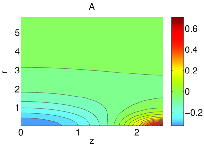
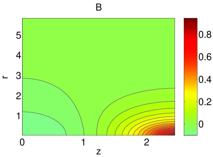
Figure 2: Contour plots of the metric functions $A,B,C$ for a perturbation with intermediate non-uniformity, $\lambda\simeq 1.2$. $B_{max}$, the value of $B$ on the horizon at $r=0$, $z=L$ is in the bottom right hand corner in the $B$ plot. Note that the gradients are largest in this corner. (Generated using $m=1$, $L=2.4758$, with grid resolution $240*100$, $dr,dz\simeq 0.025$)

In figure 3 we show a spatial embedding of the horizon for this solution. We embed the 5-dimensional spatial horizon geometry into $\mathbb{R}^{3}$, having projected out 2 of the trivial sphere directions. We also do the same for a nearly uniform string with $\lambda=0.1$ and also the most non-uniform relaxed, with $\lambda=3.9$. Hopefully this allows the reader to have a more intuitive view of the horizon geometry for different $\lambda$.

     

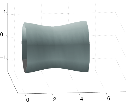
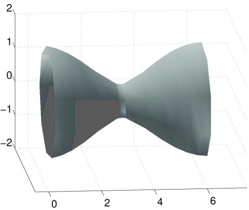
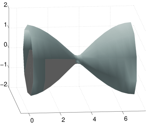
Figure 3: Embeddings of the spatial geometry of the event horizon into 3 dimensional space, projecting out the 2 trivial sphere directions. The top plot is for $\lambda=0.1$, where the leading order perturbation theory gives good results. Already for $\lambda=1.2$, the bottom left plot, the deformation is large and in the non-perturbative regime. The bottom right plot is of the most non-uniform string relaxed in this paper, having $\lambda=3.9$.

In figure 4, for the same $\lambda=1.2$ solution we plot the constraint equations, $G^{r}_{~{}z}$ and $(G^{r}_{~{}r}-G^{z}_{~{}z})$. For comparison we also plot, 2 of the 4 independent components of the Weyl tensor; $C^{tr}_{~{}~{}tr}$ and $C^{tz}_{~{}~{}tz}$. In fact we weight both the constraints and the Weyl curvatures by the explicit background $r$ dependence of the measure, $r(1+r^{2})$. We then term these quantities the ‘measure weighted constraints/curvatures’, although technically we have not really weighted by the actual measure, but only the relevant factor of it. We weight the constraints for two reasons; firstly, because this more closely resembles the quantity that enters the Bianchi identities (3), and secondly, because even tiny violations of the constraints at the horizon (which we always expect numerically) result in $1/r$ divergences. Thus multiplying by this factor of the measure converts this unphysical divergence to a finite value. Note that the indices of the Weyl components are raised and lowered as they would appear in curvature invariants, and that the $C^{tr}_{~{}~{}tr}$ component receives a contribution $3/(1+r^{2})^{2}$ from the background metric. This allows one to see the significant curvatures due to the non-uniformity, compared to the homogeneous string background, for this intermediate value of $\lambda$.

We see that the constraints are very well obeyed over the whole space. Of course, there is no well defined measure of numerical error, but a useful rule of thumb is to compare typical, and peak values of the constraints with the Weyl curvature components, which have both been multiplied by the measure factor in the same way. We see that the typical value of the weighted Weyl curvatures is of order one, and the weighted constraints are far less, their peak values being a few percent of the typical curvatures. In fact for this intermediate value of $\lambda$ we see that the majority of constraint violation is at large $r$, and results from imposing the asymptotic boundary at finite $r$. We later show (Appendix B.2) that this violation is reduced when we increase this value of $r$, $r_{max}$, and that for $r_{max}\gtrsim 6$, the metric functions are virtually unchanged by increasing it. We choose $r_{max}$ to be as low as possible, and still give good results, simply to decrease computational time. For more detailed discussion of constraint violation with increasing resolution the reader is referred to Appendix B.3. There it is shown that the numerical constraint violation does indeed improve for a given $\lambda$ as the resolution is increased, as we expect.

     

     

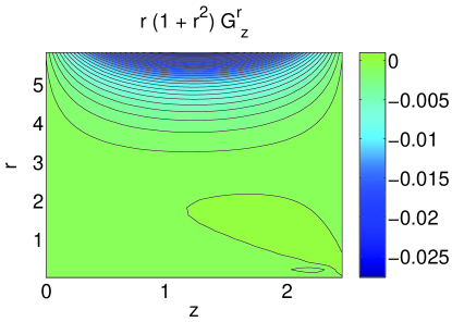
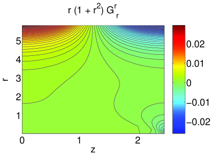
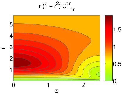
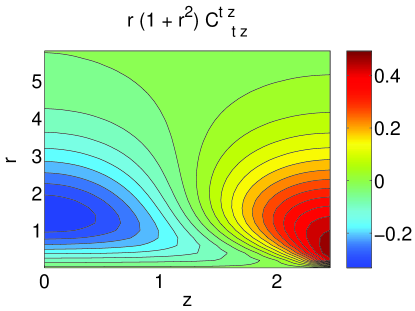
Figure 4: Top left and right: Again for $\lambda=1.2$, plots of the measure weighted $G^{r}_{~{}z}$ and $G^{r}_{~{}r}$ respectively. Note $G^{r}_{~{}r}$ is equivalent to the constraint $(G^{r}_{~{}r}-G^{z}_{~{}z})$ due to the interior equations being satisfied. These should be compared to two components of the measure weighted Weyl tensor, $C^{tr}_{~{}~{}tr}$ and $C^{tz}_{~{}~{}tz}$ on the bottom left and right, with indices as they would appear in curvature invariants. The weighted curvatures are of order one, but the weighted constraints are much smaller, showing the constraints are well satisfied, the peak constraint values being a few percent of the typical curvatures.

4.1 Self-adjustment and Consistency for Different Choices of $L$

As discussed, non-uniform solutions break the scale invariance of the uniform solutions that allows the mass per unit length and asymptotic $S^{1}$ size to be independent parameters. Fortunately our method automatically finds the correct solution without us having to tune $m$, the background mass per unit length, for a given asymptotic $S^{1}$ length $L$.

We illustrate the configurations found fixing $m=1$ and choosing different values for $L$ in figure 5. We have chosen $B_{max}=0.025$, so a very small deformation, and have chosen the critical $L=2.4758$, the value corresponding to the periodicity for small deformations for this $m=1$, and 2 other values of $L$, 20% larger and smaller. We see that the method beautifully adjusts the mass per unit length, via the static mass mode, deforming $A$ and $C$ as in (7). On top of this homogeneous background there is the very small perturbation imposed.

Thus we can compute all results using several values of $L$. Indeed we will use this method in the later section 5 to show the very good consistency of the solutions generated. This is similar to changing the ‘scheme’ in Gubser’s perturbative approach.

     

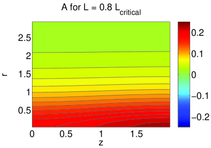
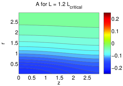
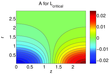
Figure 5: Plots of the metric function $A$ for $B_{max}=0.025$. We fix $m=1$, the mass per unit length of the background metric, and vary the asymptotic $S^{1}$ length, $L$. The lower plot uses the critical value $L=2.4758$. The top left uses a value of $L$ $20\%$ smaller than the critical, and the top right uses $20\%$ larger. One sees that the small perturbation in the critical case is simply superimposed on the static mass mode background for the two top plots. In these cases, the mass mode readjusts the mass per unit length so that the solution has the correct periodic length. We find we may start with any $L$ and have $m=1$, and the method works. This allows consistency checks to be made, as in the perturbation approach, and is analogous to a non-perturbative ‘change of scheme’.

4.2 Comparison with Perturbation Theory for Small $\lambda$

Another check of the method is a comparison with perturbation theory for solutions near the critical point. By changing the perturbation ‘scheme’ to fit that singled out by our conformal gauge choice and asymptotic boundary conditions, we may directly compare the two methods. The scheme that the non-linear method chooses is that the asymptotic $S^{1}$ size is fixed. In order to compare with the perturbative method we pick this asymptotic size to be the critical one for the $m=1$ background solution with $A,B,C=0$, ie. $L=2.4758$. In this scheme we must choose $C^{0(1)}$ so that $k^{(1)}=0$. This is a shooting problem that we may perform by hand and the results are given in Appendix A.

We empirically find that the absolute error in quantities calculated by our non-linear method, inferred by comparing different resolutions, is approximately constant for different $\lambda$. Therefore choosing a very small $\lambda$ to compare the perturbation theory and the non-linear method means that the quantities being measured are tiny, and thus the fractional errors will be enormous. Conversely, choosing to compare at a large value of $\lambda$ means that non-linear corrections will be large, and we only compute fully up to second order in the perturbation theory. So we choose to use $B_{max}=0.1$, corresponding to $\lambda\sim 0.1$, which is not too small, or too large. For various quantities, the following table shows the fractional differences between the value calculated in the perturbation theory and the value given by our non-linear method for 3 different resolutions.

Quantity	240*100	120*50	60*25
$\{A,B,C\}^{1(0)}$	*	*	*
$B^{0(1)}$	*	*	*
$\{A,C\}^{0(1)}$	0.06	0.16	0.64
$\{A,B,C\}^{2(0)}$	*	*	*
$\delta\mathcal{S}/\mathcal{S}$	0.08	0.40	1.87
$\delta\mathcal{T}/\mathcal{T}$	0.04	0.14	0.61
$\delta\mathcal{M}/\mathcal{M}$	0.07	0.27	1.23

Here $\mathcal{S},\mathcal{T}$ and $\mathcal{M}$ are the entropy, horizon temperature and mass of the string. The values for the metric at the horizon were calculated by Fourier transforming the solution generated by the non-linear method at the horizon, to extract the various perturbation theory contributions. We calculate $\bar{\lambda}$ from the amplitude of the $\cos(k^{(0)}z)$ component of $C$ at the horizon (as $C^{1(0)}=1$), and then use this to normalise the other components in the expansion (6). As noted earlier, the $\bar{\lambda}$ in the perturbation expansion agrees with $\lambda$, defined geometrically (5), to leading order in $\lambda$. The comparison of values in the table above can only be meaningful to leading order in $\lambda$, as only the leading order contributions were calculated in the perturbation theory. A ‘*’ indicates a small difference, of order the expected size of next order corrections, estimated by $\lambda^{2}\sim 0.01$.

Again, we wish to stress that the fractional errors shown only apply for this value of $\lambda$. It is the absolute errors that are approximately constant with $\lambda$, the fractional errors decreasing as the quantity of interest increases in magnitude. Thus the fact that the fractional error in the lowest resolution in the above table is very large for some quantities is merely a reflection of taking a small $\lambda$ so that the quantity measured is very small itself. The best way to assess errors due to finite resolution is in the later figure 6, where the same thermodynamic quantities are plotted for the 3 resolutions. We then see that the absolute errors are very small, even for the lowest resolution, $60*25$. For all quantities measured, over the whole range of $\lambda$, the 3 resolutions converge consistently with second order scaling.

It is easy to see from the table that the errors in the horizon metric functions appear to be localised in $\{A,C\}^{0(1)}$. These are the $z$ independent modes, and are responsible for the asymptotic behaviour of the solution at large $r$. The asymptotic boundary conditions discussed in section 3.1 constrain exactly these modes. In addition, $\delta\mathcal{M}/\mathcal{M}$ shows that the mass estimation carries some error too. It is technically difficult to extract the mass from the metric solution, as firstly, the $z$ independent component must be extracted by averaging at the asymptotic boundary, and then this must be integrated to large $r$ to find the mass (this is detailed in Appendix B.1). Thus the quantities with the greatest error are those associated with the large $r$ asymptotics of the solution, as we might have expected.

What is crucial is that the scaling of the errors towards the perturbation theory values with increasing resolution appears to be compatible with a second order scaling. This is exactly what we expected to find, and indicates that, at least for low $\lambda$ the method performs very well with no obvious systematics.

4.3 Large $\lambda$

Let us now turn to our primary interest, the behaviour of the solutions at large $\lambda$. The highest resolutions used in this paper allow $\lambda$ to be as large as $\sim 3.9$. The first issue is how to relax solutions with large $\lambda$.

The initial ‘guess’ configuration we relax from is very crude, simply taking the metric functions to be zero everywhere except on the horizon where we put a crude cosine function for $B$ with the correct value of $B_{max}$ at $z=L$. Note that we have also checked that for a different initial guess we obtain the same final solution. Unsurprisingly, if we start with a moderate $\lambda$, say $\lambda>0.3$, the method diverges immediately. We must gently increase the value of $B_{max}$, say in steps of $\delta B_{max}=0.05$, building up from the small values where the initial convergence does work. Thus we take the solution $B_{max}=0.30$ and then run the algorithm using this as a starting guess, but perturbing $B_{max}$ to $0.40$.

The next question is then how far we can proceed with this method. We see in figure 2 that the conformal gauge allocates more of the coordinate space to the region where $B$ is negative than positive. For large $\lambda$ we find that large numerical gradients accumulate in the $r=0$, $z=L$ corner of the lattice. For a fixed resolution, there appears to be a critical value of $\lambda$ where the constraints start to become severely violated in this corner. We believe this is simply due to the lack of resolution for the large gradients. Continuing to even larger $\lambda$ the method fails to produce a convergent solution. If we double the resolution in both $r$ and $z$, the constraints are reduced and we can proceed to higher $\lambda$ finding convergent solutions. Thus we see that this lack of convergence is simply an artifact of the algorithm. However, it does mean that we must use higher and higher resolutions to find very non-uniform solutions.

For the implementation outlined in Appendix B, a resolution of $60*25$ fails to give convergence for $B_{max}\simeq 1.2$, and as this value is approached, the constraints become increasingly violated in the $r=0$, $z=L$ corner of the lattice. Increasing the resolution to $120*50$ allows us to proceed up to $B_{max}\simeq 1.4$ before similar constraint violations occur, and convergence breaks down. To explore larger $\lambda$ we use the resolution $240*100$, the highest used in this paper, which appears to give good results up to $B_{max}\simeq 1.9$, above which convergence fails. The corresponding $\lambda\simeq 3.9$. See Appendix B.3 for detailed plots of these effects.

It is difficult to access the physical effect of the constraint violation. We might compare the weighted constraints with the weighted curvatures, as in figure 4. However, we note that the physical properties extracted from the solutions, and shown in the following sections (for example, see figure 6), agree well for measurements of different resolutions, even near the maximum $\lambda$ for the lower resolutions, where convergence breaks down and the constraints are most violated. In particular we can see this comparing $60*25$ solutions properties for $\lambda$ near the limit of convergence, with the corresponding $240*100$ solutions of the same $\lambda$, for which the constraints are very well satisfied. While the constraints are violated there, and the large gradients are not well resolved on the $60*25$ lattice, the quality of the solutions still appears to be very good. This is why we trust the $240*100$ results presented later up to the point where convergence is lost.

In principle we could proceed to higher resolution than $240*100$. However the computation time obviously increases with resolution. The algorithm was implemented using elementary numerical methods. A $240*100$ grid would take several days of relaxation time on a typical desktop PC. We discuss areas of numerical improvement in section 7 which would almost certainly make the next resolution jump accessible, allowing much larger $\lambda$ to be found. For the purposes of this paper, this is left for further research.

In summary we appear to have a consistent non-linear scheme that converges with increasing resolution, and apparently allows us to access finite values of $\lambda$ deformation. Ideally we would have hoped that we could access all available $\lambda$. Whilst this may be so, it appears that in the implementation of the elliptic method presented here, the resolution is required to increase for increasing $\lambda$ to ensure the constraints are well satisfied and convergent solutions are found. This being said, even with very modest processing power, and elementary numerical methods, we have been able to probe large finite values of $\lambda$.

5 Thermodynamic Properties of the Non-Uniform Strings

We have demonstrated a numerical method which computes the non-uniform black string geometries, and using limited resolution and computing power, have found configurations up to $\lambda\simeq 3.9$. We now discuss the properties of these solutions. In the first sub-section we consider the basic thermodynamic quantities that we can compute robustly, and show various consistency checks. In particular, we will show that the mass of the non-uniform solutions, for fixed asymptotic $S^{1}$ radius, is always greater than the mass of unstable uniform strings. In the second sub-section, we discuss quantities which are harder to determine using the numerical results we have available, due to requiring differencing of almost equal values, or division of small quantities.

5.1 Temperature, Entropy and Mass

The natural geometric properties of interest are the horizon temperature $\mathcal{T}$, the horizon volume or entropy $\mathcal{S}$, and the total mass $\mathcal{M}$, and their variation with $\lambda$. In figure 6 we fix the asymptotic $S^{1}$ length and plot these quantities normalised by their value for the critical uniform string. Three different resolutions, $60*25$, $120*50$ and $240*100$, are used to generate this data, over the ranges where the resolution still converges, and we take $m=1$ and $L=2.4758$, the critical $S^{1}$ length for this $A,B,C=0$ background. We see that for small deformation, where we can compare all 3 resolutions, the different resolutions are very consistent, and are compatible with second order scaling. Even the accuracy of the lowest resolution appears to be good. As we have mentioned, the reason to proceed to higher resolution is primarily to increase the range of convergence, rather than to increase the accuracy of the solution. Also of interest is that, for a given resolution, the last points which converge have the largest constraint violations, as outlined earlier. We do see small deviations appearing between the failing lower resolution and the higher resolutions near the end of converge of the lower resolution. However the deviations are very small, and thus we conclude that the physical error due to the constraint violations is similarly very small. Thus even near the point where the highest resolution breaks down, we believe that the curves are accurate.

These plots are the key result of this paper. The plot of the mass normalised by the critical string mass, $\mathcal{M}/\mathcal{M}_{\lambda=0}$, is the crucial one. Firstly we observe an asymptotic behaviour in $\lambda$. The mass appears to reach a fixed value as the non-uniformity becomes very large, this asymptotic mass being approximately twice that of the critical string. This indicates that the non-uniform black string cannot be the end state of the uniform string GL instability as all these non-uniform strings are more massive than the unstable uniform ones, and thus such a decay is classically forbidden. As for the uniform strings, as the mass of the non-uniform solution increases, the entropy also increases monotonically, and the temperature decreases. As with the mass, these quantities stabilise to constant asymptotic values. We discuss the implications at length in the later section 6.

We now check these results using simple consistency tests. Firstly, as discussed earlier, we may change the ‘scheme’ by choosing different values of $L$. In figure 7, we plot the same quantities as in the previous figure, using the middle resolution, $120*50$, choosing to plot the critical $L$ results, but in addition 2 values of $L$ offset by $\pm 20\%$. Overlaid on this is the high resolution curve, $240*100$, for critical $L$, over the range where the middle resolution converges. Again we see extremely good consistency. The values calculated with the critical $L$ agree for the middle and high resolutions very well as we just observed for figure 6. However the non-critical $L$ values also agree very well, the errors being small, of order a few percent.

     

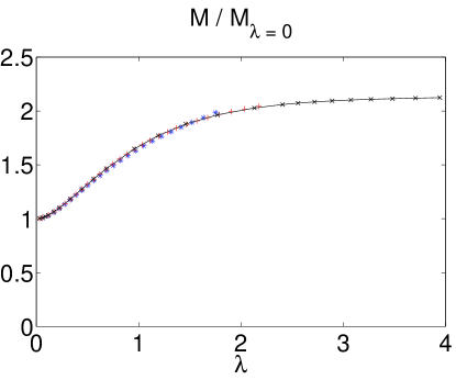
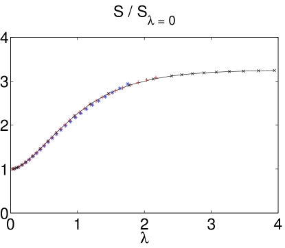
Figure 6: The key results of this paper: for fixed asymptotic compactification length, the thermodynamic quantities for the non-uniform black strings plotted against $\lambda$, normalised by their value for the critical, $\lambda=0$, string. We see that all these quantities appear to asymptote to a constant for large $\lambda$. In particular the mass is always greater than that of the critical uniform string, and therefore the non-uniform strings cannot be the end state of decay for the Gregory-Laflamme instability. Three resolutions are used, $60*25$ in blue, $120*50$ in red and $240*100$ in black. Very good consistency is found, even near the $\lambda$ where convergence breaks down for the lower two resolutions, and we would expect the lower resolution to have errors due to constraint violation. (Results generated using $m=1$ and the critical value of $L=2.4758$)

     

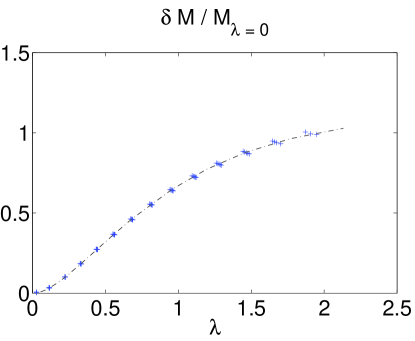
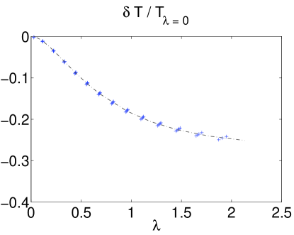
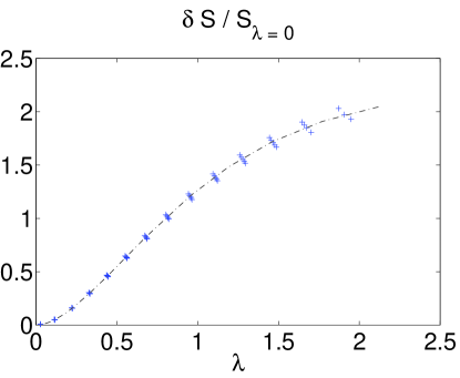
Figure 7: Again we plot the thermodynamic quantities. For the middle resolution, $120*50$, we show in blue the critical $m=1$, $L=2.4758$ scheme, but also two values of $L$ which are $20\%$ higher and lower. The high resolution $240*100$ data for the critical $L$ is shown in black. We see very good agreement to the few percent level for the scheme changing.

However, whilst $\lambda$ is large, we may still wonder how well the perturbation expansion does. Indeed in section 4.2 we showed agreement for a particular, and small, value of $\lambda$. We will now show that the behaviour near the origin in $\lambda$ agrees with the thermodynamic curves measured, but that the theory becomes fully non-linear for $\bar{\lambda}\simeq 0.5$, where $\bar{\lambda}$ is the perturbation expansion parameter, as in Appendix A.

The thermodynamic quantities $\mathcal{T,S}$ have leading order contributions $=\mathrm{const}\cdot\bar{\lambda}^{2}+O(\bar{\lambda}^{4})$, so actually the perturbation theory is accurate up to, and including, cubic order in $\bar{\lambda}$. Thus when comparing the non-linear method with the perturbation theory, we wish to determine the value of $\bar{\lambda}$ in the non-linear solutions correct to quadratic order. We could just take $\lambda$, but this only equals $\bar{\lambda}$ up to linear corrections. It is better to extract the amplitude of the $\cos{Kz}$ Fourier component of $C$, as in (6), which is indeed equal to $\bar{\lambda}$ up to quadratic corrections. We term this amplitude $\tilde{\lambda}\simeq\bar{\lambda}+O(\bar{\lambda}^{3})$

In figure 8 we firstly plot the inferred value of $\tilde{\lambda}$ from the solutions, comparing this against the actual $\lambda$. We find that $\tilde{\lambda}$ appears to asymptote to around $0.5$. This shows that near this value of $\tilde{\lambda}$ ($\simeq\bar{\lambda}$), the perturbation theory is no longer accurate, and instead the full non-linear theory must be computed. This occurs for $\lambda\gtrsim 1$ and indicates the regime where corrections to the leading order results are larger than the leading order results themselves, so all higher order corrections are potentially relevant. We might have expected that the perturbation parameter $\bar{\lambda}$ would deviate from $\lambda$ by substantial non-linear corrections before it reached one as some of the coefficients in relevant quantities, such as the entropy, are quite large. Also in the figure we plot the thermodynamic quantities measured using the highest resolution against the perturbation theory results, given in the Appendix A. As we extract $\tilde{\lambda}$, and plot the perturbation theory results as $\mathrm{const}\cdot\tilde{\lambda}^{2}=\mathrm{const}\cdot\bar{\lambda}^{2}+O(\bar{\lambda}^{4})$, these curves should be accurate to cubic order in the perturbation expansion parameter $\bar{\lambda}$, not just leading quadratic order. Indeed, we see that excellent agreement is found near the critical point.

     

     

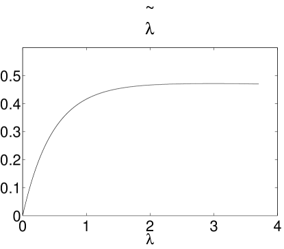
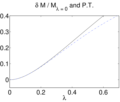
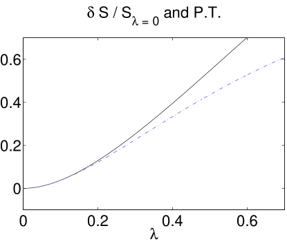
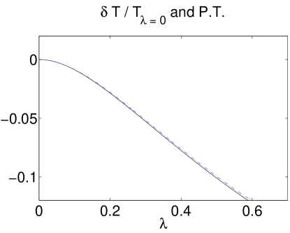
Figure 8: The top left plot shows $\tilde{\lambda}=\bar{\lambda}+O(\bar{\lambda}^{3})$, inferred by Fourier transforming the non-linear solutions at the horizon. We see that $\tilde{\lambda}$ asymptotes to approximately $0.5$, indicating that the perturbation theory breaks down for $\bar{\lambda}$ near to this value. Remaining frames show the actual thermodynamic quantities in solid black, together with the leading order perturbation theory results in dotted blue. These should agree to cubic order in $\bar{\lambda}$. We do indeed see excellent agreement near the critical point as expected.

One nice test of the constraints we may perform is to compare the asymptotic mass calculated directly from the solutions with the mass integrated from the first law. Using the first law we may compute,

$$\frac{d\mathcal{M}}{d\lambda}=\mathcal{T}\frac{d\mathcal{S}}{d\lambda}$$ (9)

where $\mathcal{S}$ is the horizon volume, or entropy, and $\mathcal{T}$ the temperature. Both $\mathcal{T}$ and $\mathcal{S}$ are easily measured from the lattice at $r=0$. On the other hand, the mass is determined by extrapolating the zero mode component of the metric, as described in Appendix B.1. The errors inherent in this mass computation not easily assessable. Therefore this provides another very useful, and non-trivial check of numerical consistency of the whole scheme. In figure 9 we plot the directly measured mass against the first law mass for the highest resolution ($240*100$). We interpolate between data points of $\mathcal{T}$ and $\mathcal{S}$ in order to calculate the necessary derivatives, and then integrate to give $\mathcal{M}$. We see satisfactory agreement, the asymptotic mass differing by about $6\%$ for the two curves.

One slightly confusing point is that plotting the same curve for the lower resolutions results in a similar difference between the two curves. We would expect that the difference should improve with resolution. Furthermore, this seems to also be independent of increasing the position of the large $r$ boundary. This strongly indicates that there is a systematic error that remains unidentified. We expect that this error lies in the asymptotic mass determination which is difficult to implement numerically. Thus we advocate using the mass integrated from the first law, assuming the error to be in the asymptotic mass, a point we return to shortly. However, whilst the error does not appear to decrease as it should, we see that the overall consistency of the two curves is good, and certainly the qualitative form of the mass relation appears very robust. Coupled with the good agreement for the perturbation theory results at small $\lambda$, and the well satisfied constraints for all $\lambda$, we believe that the systematic is likely to be a small effect, although one worthy of further investigation in future work.

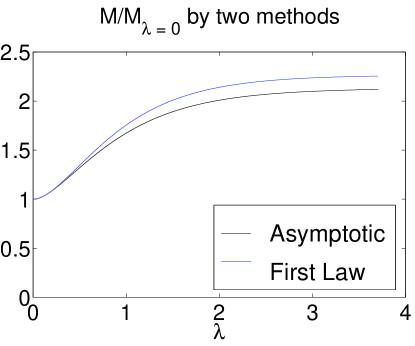
Figure 9: Plot showing the mass calculated directly from examining the asymptotic behaviour, with that computed from the horizon geometry using the integrated form of the first law. We see very good agreement, confirming that this is indeed the correct behaviour, the mass tending to a constant asymptotically in $\lambda$, which is approximately twice that of the critical string.

5.2 ‘Difficult’ Quantities: Entropy Difference and Specific Heat

We now consider quantities that are ‘difficult’ to determine accurately, the entropy (or horizon volume) difference between non-uniform and uniform strings, and the specific heat. The first is difficult to determine as we must difference two almost equal numerical quantities to compute it. The second is difficult to determine at large $\lambda$ as we must take the ratio of two quantities which both tend to zero. We will present results for the entropy difference and specific heat, as they are of interest thermodynamically. However, we wish to be clear that unlike the thermodynamic curves for $\mathcal{T},\mathcal{S},\mathcal{M}$ in the previous sub-section, which we believe to be robust, these ‘difficult’ quantities may contain some systematic errors, and therefore we do not feel we can draw concrete inferences from them.

Firstly consider the entropy of the non-uniform solution compared to a uniform string with the same mass, as in [19]. If the non-uniform solutions are found to be classically unstable, the entropy difference will indicate whether a non-uniform string can potentially classically decay to a stable uniform string of the same, or lower mass. However this involves differencing two almost equal numerical quantities, that cancel to leading order $\bar{\lambda}^{2}$, and therefore we expect it to be difficult to determine due to sensitivity to systematic error. The entropy of the uniform string with mass $\mathcal{M}$ goes as, $\mathcal{S}_{uniform}\propto\mathcal{M}^{3/2}$ and thus in order to calculate it we must know the mass. We now have two ways to compute this mass, one directly from the asymptotic behaviour of the metric functions, and the other from using the horizon geometry and integrating the mass from the first law. In figure 10 we plot the entropy difference calculated using the integrated mass from the first law, using the highest resolution. We also plot the perturbation theory to leading order in $\bar{\lambda}$, which goes as $\sim\bar{\lambda}^{4}$. Again we see excellent agreement between the two for small $\lambda$, and considering we are differencing two almost equal numerical quantities this appears to accurately reproduce the quartic behaviour in $\bar{\lambda}$. We see that the entropy difference between the non-uniform string and a uniform one of the same mass also remains monotonically decreasing and negative. Note that the entropy difference is small compared to the actual entropy of the non-uniform string. If we calculate this entropy difference using the mass computed directly from the asymptotic behaviour, we find poor agreement with the perturbation theory result near the critical point, giving more evidence to our previous claim that our direct mass calculation contains some unidentified systematic error. Whilst this is evidently small, as discussed earlier, and seen in figure 9, it is large enough to upset the computation of the very delicate entropy difference which involves differencing two almost equal numerical quantities.

     

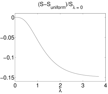
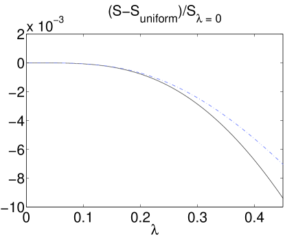
Figure 10: The difference in entropy of the non-uniform string from a uniform string of the same mass. Computed using the mass calculated from the integrated first law. The dotted curve is the leading order perturbation theory result, quartic in $\bar{\lambda}$, and gives excellent agreement near the critical point. For large $\lambda$ the entropy difference appears to asymptote to a small negative constant. If a non-uniform string is unstable, this implies that it could potentially classically decay to a stable uniform string of the same, or lower mass, provided the mass difference was relatively small.

We now consider the specific heat of the non-uniform solutions, $d\mathcal{M}/d\mathcal{T}$. It is immediately clear from the ‘robust’ thermodynamic curves 6, that the specific heat is negative. We calculate it by taking the ratio of $d\mathcal{M}/d\lambda$ and $d\mathcal{T}/d\lambda$. The reason this quantity is ‘difficult’ to determine is that at large $\lambda$ both these derivatives become small, and hence any systematic error is likely to be vastly amplified in the resulting ratio, the specific heat. In figure 11 we plot the curves yielded from both estimators of the mass, the integrated first law mass and the asymptotic metric mass. We see agreement for small $\lambda$, which we expect as the form of the two masses agree with each other, as discussed in the last sub-section, and shown in figure 9. However, we see from figure 6 that for $\lambda>2$ the derivatives of $\mathcal{M,T}$ with respect to $\lambda$ become very small, and therefore we do not have confidence in these curves beyond $\lambda\simeq 2$. We can confidently say that the specific heat initially decreases with $\lambda$. It is tempting to say it appears to asymptote to a constant at large $\lambda$, but this is highly speculative. Again this example serves to illustrate the requirement for future work that improves the mass estimation and reduces systematic errors, so that even these ‘difficult’ quantities can be managed.

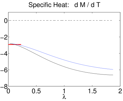
Figure 11: Plot of the specific heat measured using the mass integrated from the first law (solid black) and the mass calculated directly from the asymptotic metric (solid blue). The red bar is the value predicted by perturbation theory for $\lambda=0$, and we see good agreement there. The specific heat decreases from that of the critical string. However, asymptotically in $\lambda$ it is difficult to determine the behaviour, as both $d\mathcal{M}/d\lambda$ and $d\mathcal{T}/d\lambda$ become small and thus we expect amplified numerical errors in their ratio. Above $\lambda\simeq 2$ we expect these curves to be unreliable.

6 Discussion

The main findings of this paper are found in figure 6, namely that we can construct the compactified non-uniform string in the full non-linear theory, and that the mass is always larger than that of the critical uniform string. This appears to rule out the possibility that the Gregory-Laflamme instability can have these non-uniform strings as an end state. We have also shown that the non-uniform strings have lower entropy than uniform strings of the same mass. Unfortunately we cannot tell whether these solutions are classically stable. There are several plausible options, illustrated in the introduction in figure 1.

Firstly the solutions are classically stable. This would result in a very clear violation of black string uniqueness [39]. They are then likely to play a crucial role in higher dimensional dynamics, particularly in black hole formation in compactified extra dimensions where the black hole mass is in the range where both the uniform and non-uniform solutions exist. The behaviour would be similar to the uniform strings above critical mass. As with the uniform strings, the non-uniform solutions have monotonically increasing entropy with mass, and monotonically decreasing temperature. Quantum mechanically, we would therefore expect the compact non-uniform string to emit radiation, and adiabatically move to a lower mass non-uniform string, until the critical point is reached when the classical instability will occur. Thus the radiation carries away mass and entropy from the string, and in the process reduces its non-uniformity.

Secondly the strings are dynamically unstable, as advocated by Kol [7]. If this is the case, it would then be improbable that the non-uniform solutions would play much role in the dynamics of gravity in higher dimensions, simply because it is unlikely any initial data would evolve to a state near these static solutions. However, it is again interesting to consider the classical decay of such a solution. The dynamics of the classical instability would then be governed by the nature of the dominant unstable mode, and the amount of radiation emitted in the process. If little radiation is emitted, we could conceive a non-uniform string classically decaying to a uniform stable solution with slightly less mass. This is amusingly reminiscent of the Horowitz-Maeda expectation, but now in reverse, the unstable non-uniform strings decaying to the stable uniform ones. Note that as we have shown the horizon volume, or entropy, of the non-uniform solutions is less than that of the uniform solutions with the same mass, this process is allowed by the second law. However, since this horizon volume difference is small, it also means that the mass lost to radiation must also be small. The volume difference allows a transition to an equal mass uniform string, but the horizon volume of less massive uniform strings decreases, and if too much mass is lost, the process would then violate the second law. The alternative is that the decay is to the same end state that the unstable uniform strings reach, whatever that might be. Note that if much radiation is emitted due to the classical instability, then as argued above, the latter case is the only option.

The only arguments concerning classical stability are those made by Kol in the interesting paper [7], claiming the simplest picture is for the strings to be unstable. This is largely based on assuming that thermodynamic instability implies classical instability. Whilst this is shown [13, 14, 16] in the uniform case, translational invariance is critical in the argument, and there is no evidence that the relation should be more general. Thus we feel that their classical stability is very much an open, and interesting question. It also remains an interesting question whether this branch of non-uniform string solutions connects with the branch of compactified black hole solutions, as suggested by Kol [7]. In a future work, we will look at the geometry of our non-uniform string solutions to infer whether it is plausible that these two branches of solutions are linked.

The best way to understand the dynamics of the black strings is simply to solve the full time dependent equations. Whilst this appears to be under way, the end state of the full dynamical simulations is apparently still inconclusive [20, 21]. From the results presented here, we expect that the end state is not a non-uniform string, at least in the branch of solutions connected to the GL critical point. This could considerably complicate the long term dynamical evolution. The best possibility from the numerical point of view would have been an adiabatic motion to a non-uniform string solution. Then all curvatures, and time derivatives would have remained small during the simulation. Gubser showed that this was not the case. The next best case would have been a brief non-adiabatic period and then a slow motion to the non-uniform string. Presumably the more dramatic the evolution, the harder it is to evolve for long times. However, the present work indicates a different end state all together, and so it could be that large curvatures and long dynamical times may be involved in uncovering this end state, probably making the numerical problem considerably more tricky.

Let us finally comment briefly on the interesting work of Harmark and Obers [23]. As mentioned in the introduction they have an ansatz that may solve the Einstein equations in terms of only one unknown function. This is shown to be a consistent ansatz to second order in an asymptotic expansion, which is highly non-trivial evidence supporting their claim. However the resulting equation for the unknown is not pleasant, and would almost certainly require numerical solution. It is then very interesting whether we could apply the methods of this paper to the solution of their equation, and whether this would give a simpler method than the one using the conformal gauge we use here. At first sight having only one function to solve for would appear to be beneficial. However, really it is not the number of equations to be solved that is critical, but rather the stability of the equations under some relaxation algorithm. The powerful feature of our method is that because the conformal gauge equations for the metric functions have Laplace second derivatives, at least for small non-uniformity solutions can be easily found by a very simple relaxation algorithm. Thus the fact that we have more than one equation to solve, due to our 3 metric functions does not really complicate the method. In the Harmark and Obers ansatz, reducing the metric to only one function involves substituting a metric function that can be determined algebraically. This results in third order derivative terms. It would be interesting to see whether standard techniques could be used on this equation. We think it is likely to be better to not eliminate the second function, and stick to reducing the problem to two metric functions, and solving for these. Either way, it appears that our methods might be applied. This could allow the consistency of the ansatz to be tested. If correct, the ansatz may provide a powerful way to implement these elliptic methods.

7 Other Applications and Areas of Improvement

The guiding principles we have used in applying the elliptic method of solution are the following:

• Perturb about a background solution, such that the deformation is parametrised by finite valued metric functions.

• Choose a problem where at least some of the boundaries have data that is implemented locally, ie. not involving integration over a boundary, or worse, integration from one boundary to another. In the Randall-Sundrum star case [26] the metric perturbation decayed to zero far from the brane and this satisfied the weighted constraints. On the brane one non-local integration was performed. In the present example 2 boundaries, $z=0,L$, are periodic, and the asymptotic boundary has simple local boundary conditions. Only the horizon boundary requires a non-local integration operation.

• Most importantly, if one can solve the linear deformation problem elliptically in the conformal gauge, one should be able to use the non-linear methods employed here. Thus the method provides a way to extend static linear perturbation theory into the non-linear regime.

There are potentially numerous applications of this method. For example, one can apply it to any axisymmetric problem in more than 4 dimensions, or indeed any situation where one has static configurations with metric dependence on 2 variables. If possible, extending these ideas to allow dependence on more than 2 variables would allow insight into solutions to gravity where there is little analytically known.

One exciting avenue for future research is to understand how to include localised horizons in the scheme, which would allow access to uncharged black hole solutions in Kaluza-Klein theory, and on branes, if the latter solutions do indeed exist, (although the converse has recently been conjectured by Tanaka [40] and elaborated on in [41]). In the Randall-Sundrum star case we tackled a problem with a regular geometry and no horizon (other than the asymptotic AdS horizon). In the current work, a continuous horizon was considered. The challenge would be to understand how to merge these two situations to allow localised horizons that do not extend along the length of the symmetry axis.

Let us briefly consider the problem of a small neutral Kaluza-Klein black hole. Using a background metric that is flat space deformed by $A,B,C$ in the conformal gauge, would not allow such solutions to be found, as $A\rightarrow-\infty$ on the horizon. Large deformations of $A,B,C$ away from zero would most likely destroy the convergence of the scheme. In this paper, we are able to tackle a horizon geometry because we encoded the vanishing behaviour of the lapse at the horizon in the background metric (4), essentially as we know the translationally invariant black string solution. Then the deformations of this required everywhere finite $A,B,C$. For a localised black hole we similarly need to find a metric to perturb around that encodes the horizon behaviour. The problem is that no solutions are known. Thus, we must find a good guess, such that the solutions will require non zero, but finite $A,B,C$. An interesting guess we might try is the 5-dimensional Schwarzschild metric in isotropic coordinates,

$$ds^{2} =-\left(\frac{m-\rho^{2}}{m+\rho^{2}}\right)^{2}dt^{2}+\left(1+\frac{m}{\rho^{2}}\right)^{2}\left(dr^{2}+r^{2}d\Omega_{2}^{2}+dz^{2}\right)$$

$$\rho^{2} =r^{2}+z^{2}$$ (10)

which presumably closely approximates the horizon geometry for a very small black hole. We see immediately that $B-C=0$ for this metric, which would be important due to the singular nature of the gauge at $r=0$ where the axis of symmetry is regular away from the horizon (as discussed in [26]). So we might try the ansatz,

$$ds^{2}=-\left(\frac{m-\rho^{2}}{m+\rho^{2}}\right)^{2}e^{2A}dt^{2}+\left(1+\frac{m}{\rho^{2}}\right)^{2}\left(e^{2B}(dr^{2}+dz^{2})+e^{2C}r^{2}d\Omega^{2}\right)$$ (11)

We would hope that for a solution with small mass compared to the compactification scale, $A,B,C$ would be small. Note that due to the conformal invariance in $r,z$ there is coordinate freedom to choose the horizon to remain at the location $r^{2}+z^{2}=m$. On the horizon itself, a constant temperature condition and regularity would be imposed, just as for the black strings here. Whether such methods can be employed, and whether the solutions exist remain exciting avenues of research.

The numerical algorithms and computational power employed to produce the results in this paper were very modest. The largest area of potential improvement is in these numerical algorithms. This is particularly important in progressing to higher values of $\lambda$ where we see that already the resolution $240*100$ is not sufficient for $\lambda\gtrsim 3.9$. The time needed to relax still higher resolutions using the elementary methods of this paper is prohibitive.

There are two potential remedies for this problem. Firstly using higher order discretisation algorithms to increase the accuracy of the solutions may well mean that lower resolutions are required to capture a given $\lambda$. Alternatively, if we cannot remove the high resolution requirement, using more sophisticated relaxation algorithms might substantially reduce the time taken. For instance, we might change the Gauss-Seidel relaxation discussed in the Appendix B, to a multi-grid algorithm. Whilst it is absolutely clear that multi-grid vastly out-performs Gauss-Seidel as a Poisson equation solver, it is not at all clear that it will perform so well in our context, where the source terms and boundary conditions are iteratively updated as functions of the metric. In any case, a better understanding of the convergence properties of the method would certainly be useful.

In addition to this, we have used a regular lattice to cover the $r,z$ space. We have seen that the gauge gives rise to large gradients in the $r=0$, $z=L$ corner of the grid, which then require high resolution. However, using a variable grid spacing, or even an adaptive mesh, we might hope to concentrate points in the areas with strong gradients and thereby use the grid points more efficiently. Furthermore, at large $r$, where the solutions tend to the $z$ independent asymptotics, we could possibly use less lattice points, as the $z$ gradients would be small. Any reduction in the number of lattice points is likely to make a huge difference to the relaxation times.

8 Conclusion

We have developed elliptic numerical methods to find static axisymmetric vacuum solutions in more than 4 dimensions, where no analytic solutions are known. The method is applied to the case of the 6 dimensional compactified non-uniform black string, where the implementation is straightforward compared to our previous work [26]. We show using perturbation theory that the 6 dimensional string has the same thermodynamic behaviour as Gubser found for the 5 dimensional one near the critical point. The full non-linear method produces solutions, the relaxation time required increasing with increasing non-uniformity. We have configurations with large non-uniformity, where $\lambda\simeq 3.9$, but this can no doubt be improved by further investigation of the numerical algorithm, and use of more sophisticated numerical methods. Such values of $\lambda$ are well beyond the reach of a perturbative approach, the corrections to the leading order being of order the quantity under consideration, and thus all higher order corrections are likely to be important.

The quality of the solutions is checked in several ways. The local constraint violation is assessed, and shown to be small, and to improve with increasing resolution. The solutions are checked against the perturbation theory for small $\lambda$, and excellent agreement is found. The ADM mass of the solution can be determined directly, and via the horizon geometry using the first law, and these compare well. Thus we claim, with confidence, that the mass of the non-uniform strings is greater than that of the critical string for a given asymptotic $S^{1}$ size. A further check is that solutions can be relaxed with different asymptotic $S^{1}$ lengths, in an analogous manner to the scheme changing used by Gubser in the perturbation theory calculation. Solutions with substantially different $L$ are found to give thermodynamic curves which are highly consistent. Overall, the method appears to perform extremely well, giving good accuracy.

The mass of the non-uniform strings is robustly shown to increase with $\lambda$, asymptoting to approximately twice the mass of the critical string for very large $\lambda$. This intriguingly implies that these stable non-uniform strings are not the end state of the dynamical Gregory-Laflamme instability, and again raises the interesting question of what this end state actually is. It may well be that full dynamical numerical simulation is the only way to determine this, although if the end state, or intermediate configurations, are highly curved this may be an extremely difficult problem. We also give evidence that the entropy of the non-uniform solutions is always less than that of the uniform solutions with the same mass, although this is less firm, as we must difference two almost equal quantities to calculate this.

Unfortunately we cannot assess the classical stability of the solutions. If they are stable, our results indicate they will behave in a similar way to the stable uniform solutions, and simply Hawking radiate to the critical point. They would potentially play a crucial role in dynamics, particularly for black hole formation in theories with compactified extra dimensions when the black hole mass fell in the range where both uniform and non-uniform solutions existed. If unstable, they are unlikely to play a significant role in higher dimensional dynamics. Starting with such a solution, it might either classically decay to a stable uniform solution, or undergo the same type of decay as the uniform unstable strings. The first possibility is allowed by the second law, although the mass lost to radiation in the decay must be small.

We have discussed possible improvements for the numerical algorithms described here. We expect they can always be generalised to static problems with symmetry such that the metric depends only on two coordinates. The methods may be extendible to dependence on more than just two coordinates. An interesting future application of the method is to explicitly construct the Kaluza-Klein black hole in 5 or more dimensions. We have discussed some technical subtleties involved, and their possible solution. This open problem is complementary to studying the black strings, and understanding the compactified black hole solutions may also shed light on the dynamics involved in the Gregory-Laflamme instability.

Appendix A Appendix: Perturbation Theory and Asymptotics

In this Appendix we review Gubser’s perturbation theory method [19], and apply it to the 6-dimensional case. The Mathematica code used to generate results stated in this section will be made available [29].

We Fourier decompose the metric as in equation (6). As Gubser discusses, different values of $K$ correspond to different ‘schemes’. Geometrically, we might use this freedom to choose the asymptotic size of the $S^{1}$ to be of fixed proper length, as is relevant for comparison with our non-linear method. Another scheme, the ‘standard scheme’, allows $K$ to vary, and instead fixes $C^{n(m)}=0$ for $m\geq 2$. This scheme reduces the number of quantities that we must ‘shoot’ for, although it has no obvious geometrical interpretation.

Having fixed a scheme, the Einstein equations reduce to a series of ordinary differential equations for $X^{n(m)}_{i}(r)$, the higher orders in $\bar{\lambda}$ depending on the solutions obtained from the lower orders. At each order some of the equations are shooting problems, solved by demanding the metric functions tend to zero asymptotically and have behaviour at the horizon to ensure regularity. By Taylor expanding about the origin we obtain the condition that in the conformal gauge, the $r$ derivative of $X^{n(m)}_{i}(r)$ must vanish at $r=0$.

The quantities of interest can be determined with high accuracy, typically with consistency better than $1\%$ up to third order for scheme changes of $C^{0(1)}=\pm 1$. The same methods used to generate the 6 dimensional results below were also used to recreate the 5 dimensional results. Careful handling of the asymptotic behaviour of the ‘zero modes’ is crucial to obtain high precision and we find a final ‘scheme error’ in the entropy difference, $\sigma_{2}$ in Gubser’s terminology, of only $1\%$ for the 5-dimensional string. In fact we find a slightly better result in the 6 dimensional case, which may be attributable to the faster fall off of the zero modes asymptotically.

Having employed Gubser’s method in 6 dimensions, we now give the ‘standard scheme’ numbers for completeness, giving partial results for third order;

$$A^{1(0)}(0) =-0.783 B^{1(0)}(0) =-0.783 C^{1(0)}(0) =1$$

$$k^{(0)} =1.269$$

$$A^{0(1)}(0) =0.63 B^{0(1)}(0) =0.91 C^{0(1)}(0) =0$$

$$A^{2(0)}(0) =0.64 B^{2(0)}(0) =0.64 C^{2(0)}(0) =-0.87$$

$$A^{1(1)}(0) =-0.38$$

$$k^{(1)} =1.02$$ (12)

The numerics verify the asymptotic behaviour we expect from the zero mode equations. These zero mode components, $X^{0(1)}_{i}(r)$, do not require shooting, going as,

$$A^{0(1)} \rightarrow a_{0}\frac{1}{r^{2}} a_{0} =-0.93$$

$$B^{0(1)} \rightarrow b_{0}\frac{1}{r^{2}} b_{0} =0.65$$

$$C^{0(1)} \rightarrow c_{0}\frac{1}{r^{2}}+c_{1}\frac{1}{r} c_{0} =-0.37,\qquad c_{1}=1.69$$ (13)

where both $A^{0(1)}$ and $B^{0(1)}$ can be shifted by additive constants, and are chosen to be zero asymptotically. The components which depend on $z$ have exponentially growing and decaying solutions. The method of shooting selects the decaying solution and thus the asymptotic behaviour is dominated by the zero mode components above. This is the same as in Kaluza-Klein theory where the leading contribution to the reduced propagator is derived from the homogeneous modes, and the inhomogeneous massive modes are Yukawa suppressed at large distances.

Computation for the scheme where $k^{(1)}=0$, and thus the asymptotic size of the $S^{1}$ is held constant, yields,

$$A^{0(1)}(0) =-0.17 C^{0(1)}(0) =0.80$$

$$A^{1(1)}(0) =-0.38$$

$$k^{(1)} =0.00$$ (14)

and,

$$A^{0(1)} \rightarrow a_{0}\frac{1}{r^{2}} a_{0} =-1.73$$

$$C^{0(1)} \rightarrow c_{0}\frac{1}{r^{2}}+c_{1}\frac{1}{r} c_{0} =0.43,\qquad c_{1}=1.69$$ (15)

where we have only reproduced the quantities in (12) and (13) which are scheme dependent. These numbers can then be directly compared with those of the non-linear method which uses this scheme.

The ADM mass, $\mathcal{M}$, can be evaluated using the Hawking-Horowitz expression [42]. To leading order this gives the scheme independent quantity $\eta$,

$$\frac{\delta\eta}{\eta} =\frac{\delta\mathcal{M}}{\mathcal{M}}+2\frac{\delta K}{K}\simeq\bar{\lambda}^{2}\left(\frac{10}{3}b_{0}+2c_{0}+2\frac{k^{(1)}}{k^{(0)}}\right)$$

$$=3.03\bar{\lambda}^{2}$$ (16)

In our non-linear method, we fix the length of the $S^{1}$ for all solutions, and thus $\delta K=0$, and $\delta\eta/\eta=\delta\mathcal{M}/\mathcal{M}$. We may evaluate the horizon temperature $\mathcal{T}$, as a scheme independent quantity, $\alpha$,

$$\frac{\delta\alpha}{\alpha} =\frac{\delta\mathcal{T}}{\mathcal{T}}-\frac{\delta K}{K}\simeq\bar{\lambda}^{2}\left(A^{0(1)}(0)-B^{0(1)}(0)-\frac{k^{(1)}}{k^{(0)}}\right)$$

$$=-1.08\bar{\lambda}^{2}$$ (17)

and similarly for the horizon volume, and thus entropy $\mathcal{S}$,

$$\frac{\delta\mathcal{S}}{\mathcal{S}}+3\frac{\delta K}{K} \simeq\bar{\lambda}^{2}\left(B^{0(1)}(0)+3C^{0(1)}(0)+\frac{1}{4}(B^{1(0)}(0)+3C^{1(0)}(0))^{2}+3\frac{k^{(1)}}{k^{(0)}}\right)$$

$$=4.55\bar{\lambda}^{2}$$ (18)

Using the first law as in [19], this allows us to calculate the difference in entropy between the deformed string and a uniform string with the same mass, as is relevant in a dynamical context. Indeed we find that,

$$\frac{\mathcal{S}_{\mathrm{deformed}}-\mathcal{S}_{\mathrm{uniform}}}{\mathcal{S}_{\mathrm{uniform}}} =-\frac{3}{4}\left(\frac{d\alpha}{\alpha}\frac{d\eta}{\eta}+\frac{1}{2}\left(\frac{d\eta}{\eta}\right)^{2}\right)$$

$$=-0.98\bar{\lambda}^{4}$$ (19)

and thus the deformed string has a lower entropy. Therefore we find the same qualitative features in 6 dimensions as Gubser found in 5 dimensions, namely that for fixed asymptotic $S^{1}$ radius, the mass increases with $\bar{\lambda}$, and this entropy difference is negative. We can compute systematic ‘errors’ in the quantities presented above, obtained by recalculating the quantities in a different scheme such that $C^{1(0)}=\pm 1$. This allows us some indication of the accuracy of the method. The standard deviation of the scheme independent quantities above for $C^{1(0)}={0,\pm 1}$ are all well below $1\%$, the errors growing for higher order quantities, the largest scheme error being for the entropy difference giving $0.1\%$.

Appendix B Appendix: Technical Details

We now discuss the numerical scheme in a little more detail, and in particular the algorithm for updating the boundary data. We begin with the most time consuming step in the iteration, which is the relaxation of the interior equations.

The 3 elliptic equations are solved by splitting the Laplacian term from the source term as in (2). A relaxation scheme is used to partially relax the Poisson equations holding the sources constant. We use Gauss-Seidel combined with under-relaxation. The Gauss-Seidel method is a local update procedure, and our general philosophy in finding a stable method to solve these equations is to keep operations as local as possible. Thus, whilst non-local solvers such as multi-grid may give quicker solutions, we also expect them to be less stable in generating a convergent solution to this complicated non-linear problem.

We find that standard Gauss-Seidel works well for the $A,C$ equations. However we use under-relaxation for $B$, where the update for $B$ is,

$$B_{update}=(1-\epsilon)B_{old}+\epsilon B_{new}$$ (20)

where $B_{old}$ is the old value of $B$ at some point, $B_{new}$ is the result of the Gauss-Seidel iteration and $B_{update}$ is the updated value at the point. Thus for $A,C$, $\epsilon=1$ and there is no added ‘inertia’. For $B$ we find the method is unstable unless ‘inertia’ is added, and a value of $\epsilon=0.01$ was used for the results calculated in the paper. Understanding the nature of this numerical instability in $B$ may be crucial for improving the technique.

After one pass of Gauss-Seidel, the boundary conditions are updated, as described below. We could update the Poisson source terms every cycle, but it takes time to do so. The relaxation procedure is very simple and quick, involving little floating-point arithmetic. However, calculating the sources involves intensive arithmetic. Thus we have found that updating the sources one in ten iterations is a good compromise.

The horizon boundary conditions are that $A_{,r}=C_{,r}=0$ and that $A_{,z}=B_{,z}$. We difference $A_{,r}$ and $C_{,r}$ to second order and these allow the boundary value to be determined at $r=0$. The condition for $B$ is implemented by using a simple second order integration from the $r=0$, $z=L$ lattice point, whose value is an input parameter and specifies $B_{max}$, down to $r=0$, $z=0$. As with the interior relaxation, we cannot directly inject the integrated value. We integrate along the boundary, storing the new values in a buffer, and then inject them as in (20). Again a value of $\epsilon=0.01$ was used to generate the results in this paper. For larger $\epsilon$ the method becomes unstable.

The periodic boundaries at $z=0,L$ are updated for $A,B,C$. Differencing the zero normal gradient condition gives an update value for the boundary points, but it is again important to introduce ‘inertia’ in the update. A value of $\epsilon=0.02$ was used to generate the results presented here. Without this inertia, the solutions do not converge.

On the asymptotic boundary, we impose the conditions that $A,B\sim 1/r^{2}$ there. This is differenced to second order and the update requires no ‘inertia’. The metric function $C$ is updated by evaluating the linearised $G^{z}_{~{}z}$ constraint equation at the midpoint of the boundary, $z=\frac{L}{2}$, and ignoring $z$ gradient terms. Thus we assume that the metric functions are small and that only the $z$ independent component remains in the metric asymptotically. Picking the mid point, $z=\frac{L}{2}$, reduces any error from the exponentially suppressed $z$ dependent components in the metric, as they go as $\cos{\pi z/L}$ to leading order. This linearised constraint then yields a boundary value for $C$. We use this to determine $C$ all along the $r=r_{max}$ boundary, again assuming $z$ independence there. These $C$ values are injected with ‘inertia’, with a value of $\epsilon=0.01$ giving good results. Choosing no inertia again destroys convergence.

The above method is then iterated. After a hundred steps or so, the error in the 3 elliptic equations is calculated, being taken as the absolute of the difference of the left-hand side and right-hand side of (2). This is then averaged over the lattice for each metric function. Relaxation is stopped when these quantities are less than $\sim 10^{-9}$, and the solutions have converged.

As an initial guess for the relaxation procedure we simply take all the metric functions to be zero, and put a cosine form for $B$ on the horizon points with the correct amplitude. This appears to be quite brutal but does indeed work for deformations with $B_{max}\leq 0.3$. After this value, larger $\lambda$ solutions are best calculated by taking the relaxed solution for a lower $\lambda$, and then simply updating the value of $B$ at $r=0,z=L$ to the new $B_{max}$ value. This initial data will then relax provided that the jump in deformation is not too great. Typically we found that a jump of $\Delta B_{max}<0.15$ gives good results for all the resolutions used here. Note that perturbing the initial guess does not effect the end solution, and thus there do not appear to be any additional static perturbation modes present for the non-uniform strings.

The lattice used to cover the $rz$ plane is rectangular, with even spacing $dr,dz$ in the $r,z$ directions. We discretise the fields over the lattice as $X_{(i,j)}$ where $i,j$ are the $r$ and $z$ positions respectively and run as $i=1,2,\ldots i_{\rm max}$, $j=1,2,\ldots j_{\rm max}$. The interior equations are differenced using standard second order templates, and the Laplace second derivative terms imply they are naturally evaluated at $(i,j)$. When evaluating the constraint equations, to check the consistency of the solutions, the constraints are evaluated naturally at different lattice positions due to their second derivative structure. The constraint equation $G^{r}_{~{}z}$ contains terms taking the generic form,

$$\partial_{r}\partial_{z}X+a\,\frac{1}{r}\partial_{r}Y+b\,\partial_{r}X\partial_{z}Y+\ldots=0$$ (21)

where $X,Y$ are some metric functions. This is then evaluated at the centre of a lattice cell $(i+\frac{1}{2},j+\frac{1}{2})$, compatible with the second order mixed derivative operators. Similarly the Einstein tensor components $G^{r}_{~{}r}$ and $G^{z}_{~{}z}$ reside naturally at $z=z_{i+\frac{1}{2},j}$ and $z=z_{i,j+\frac{1}{2}}$ respectively, as indicated by their highest derivative operators, the first having only first order $r$ derivatives and the second, only first order $z$ derivatives. This is why we use $G^{z}_{~{}z}$ to determine $C$ on the asymptotic boundary, rather than $(G^{r}_{~{}r}-G^{z}_{~{}z})$.

B.1 Mass Determination and Asymptotic Boundary Conditions

In this section we discuss the asymptotic boundary conditions and how to compute the asymptotic mass from the metric at the large $r$ boundary.

In order to determine the mass of the solutions we assume that the solution at $r=r_{max}$ has no dependence on $z$. The remaining $z$ independent metric component may then be integrated out to large $r$ to determine its asymptotic behaviour. At very large $r$, we may linearise in the deformation, and then obtain the following general asymptotic behaviour of the metric (similar to in Appendix A),

$$A\simeq a_{0}+\frac{a_{2}}{r^{2}}+O(\frac{1}{r^{3}})$$ (22)

$$B\simeq b_{0}+\frac{b_{2}}{r^{2}}+O(\frac{1}{r^{3}})$$

$$C\simeq b_{0}+\frac{c_{1}}{r}+\frac{c_{2}}{r^{2}}+O(\frac{1}{r^{3}})$$

This form of the asymptotic metric yields a mass per unit length, $\rho$, of

$$\rho\propto\frac{3}{2}+5b_{2}+3c_{2}$$ (23)

to linear order in the metric, and the total mass $\mathcal{M}=\rho\,L$. At $r=r_{max}$, where we take $r_{max}\gtrsim 6$, we impose the asymptotic boundary conditions on the lattice, namely we aim to have $a_{0},b_{0}$ be zero, and to satisfy the constraint $G^{z}_{~{}z}$. However, whilst at $r_{max}=6$ we have largely eliminated the exponentially growing $z$ dependent components of the metric, it is not large enough that the $z$ independent component satisfies the above asymptotic scaling very accurately, mainly due to the slow $1/r$ behaviour in $C$. Thus we cannot extract $b_{2},c_{2}$ at this boundary directly. Really the lattice would have to extend out to $r\sim O(1000)$ to be in the true asymptotic regime. So, the metric functions and their $r$ derivatives are averaged over the large $r$ boundary. These averaged values are then integrated out to large $r\simeq 1000$, and the asymptotic values of $b_{2},c_{2}$ are determined by fitting functions of the general form in (B.1). Then the mass is calculated.

Note that we have linearised the update equation $G^{z}_{~{}z}$ for determining $C$ on the $r_{max}$ boundary, and use the scaling, $A,B\simeq 1/r^{2}$ which is based on the linear theory asymptotics. Interestingly, we find best results when the equations used to evolve the $z$ independent metric components out to very large $r$ are not linearised in the metric perturbation. Although at the asymptotic boundary the metric functions are small, even for large $\lambda$ solutions, non-linear corrections do appear to be important when integrating the $z$ independent component out to very large $r$, and do make a significant difference to the mass calculated from this asymptotic metric.

As we have imposed boundary conditions at finite $r\simeq 6$, they will not strictly enforce $a_{0},b_{0}=0$ due to the approximate nature of the boundary conditions, which really are only valid at very large $r$. However, we find in practice only a very small $a_{0},b_{0}$ which does not concern us at all, and is simply a slight change of scheme. The change of scheme is minute and can be neglected when we determine the properties of the solutions.

B.2 Finite Large $r$ Boundary Check

In this section we test the sensitivity of the solutions to the finite position of the asymptotic boundary, $r_{max}$. In the table below we compare two asymptotic quantities, the mass (measured directly) and the peak value of the measure weighted constraint $G^{r}_{~{}z}$ evaluated at $r=r_{max}$, and two horizon quantities, the horizon volume or entropy $\mathcal{S}$, and the same constraint evaluated at $r=0$. These are compared for solutions with $B_{max}=0.1$ (so $\lambda\simeq 0.1$) for different asymptotic boundary positions, $r_{max}$. All solutions are at the same resolution as for $120*50$ with $r_{max}=6$, namely $dr,dz\simeq 0.05$.

$r_{max}$	$\mathcal{S}$	weighted $G^{r}_{~{}z}$ at $r=0$	$\eta$	weighted $G^{r}_{~{}z}$ at $r_{max}$
4.0	0.04330	0.003550	0.02848	0.048406
5.0	0.04850	0.000520	0.03190	0.020042
6.0	0.04905	0.000459	0.03225	0.007933
7.0	0.04908	0.000498	0.03226	0.002682
8.0	0.04907	0.000505	0.03224	0.000918
9.0	0.04905	0.000505	0.03223	0.000306
10.0	0.04904	0.000505	0.03221	0.000100

We see that increasing the position of the boundary does indeed yield less asymptotic weighted constraint violations. The boundary conditions imposed at $r=r_{max}$ are linearised and assume that the metric is $z$ independent. This assumption obviously proves to be good enough in practice by $r_{max}=6$. The asymptotic mass, measured directly, also tends to a constant as expected, and appears to give a result close to the asymptotic value for $r_{max}\simeq 6$. We see that the entropy evaluated at $r=0$, and indeed other horizon geometric quantities, and the weighted constraints evaluated at $r=0$, are quite insensitive of the boundary position provided it is above $r_{max}\gtrsim 6$.

We thus find the required insensitivity of the solutions to the value of $r_{max}$ provided $r_{max}\geq 6$, and $r_{max}\simeq 6$ does give good results, whilst not requiring excessive relaxation times.

B.3 Constraint Violation

In this section we simply characterise the constraint violation of the solutions for varying $\lambda$ and resolution, in order to demonstrate the validity of the large $\lambda$ solutions. In figure 12, we show the measure weighted constraint $G^{r}_{~{}z}$ for 2 resolutions, medium ($120*50$), and high ($240*100$) with $B_{max}=1.25$ (so $\lambda\simeq 1.8$). Above $B_{max}\simeq 1.40$ the $120*50$ resolution no longer converges, and at this $B_{max}=1.25$ the constraint violation becomes large near $r=0,z=L$. We show the constraint over the whole lattice for reference, but it is the constraint in the lower right corner, $r=0,z=L$ that is substantially improved by going to higher resolution. This lower right corner is plotted for the two resolutions to show the improvement.

     

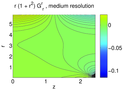
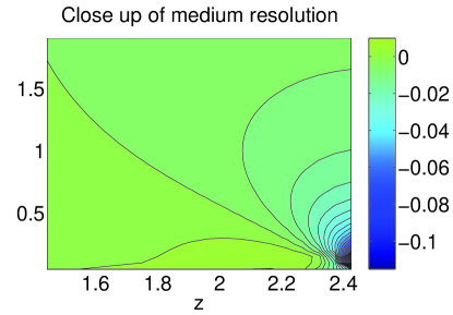
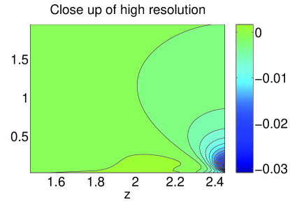
Figure 12: The top plot shows the measure weighted constraint $G^{r}_{~{}z}$ for the medium resolution $120*50$ over the whole lattice for $B_{max}=1.25$, so $\lambda\simeq 1.8$, near the point where this resolution no longer converges. The bottom left plot shows a close up of the lower right corner of the lattice, where the constraints become increasingly violated as this convergence limit is reached. The bottom right plot shows the same quantity, for the same $B_{max}$, but with the high resolution $240*100$. We see that the constraints are improved by a factor of approximately four, compatible with second order scaling. The peak value of this function is plotted in the following figure 13 for a range of $\lambda$.

This constraint violation can be characterised by taking the absolute peak value of the measure weighted constraints in the lower half of the lattice, thus picking out the trouble spot near $r=0$, $z=L$. In figure 13 we plot this peak violation value for varying $\lambda$ and for 3 grid resolutions. Note that the constraint violation in the upper half of the lattice is due to the position of the large $r$ boundary and is uneffected by changing resolution.

Firstly we see that increasing the resolution does indeed reduce these values, indicating that the constraints improve, as we would hope for. Indeed for each doubling of resolution, the constraints improve by approximately a factor of 4, indicating second order scaling, consistent with our second order differencing. Furthermore, we can clearly see the effect discussed in section 4.3, where at some large value of $\lambda$ the constraints become strongly violated at a fixed resolution before convergence is lost, and we must proceed to a higher resolution to continue to larger $\lambda$. It is always difficult to assess how physically bad a constraint violation is. The absolute values of these measure weighted constraints can be compared to the typical values of the similarly weighted curvatures. These typically take values of order one, as shown in the earlier figure 4, and thus the violation in the constraints, even for $B_{max}$ quite near to the loss of convergence point, is much smaller than the curvatures. However a more physical error assessment is to compare the thermodynamic properties of a solution at low resolution with large constraint violation, with a higher resolution where the constraints are much better satisfied. For example, comparing the temperature, mass and entropy for the low and high resolutions for $B_{max}\simeq 1.25$ ($\lambda\simeq 1.8$) where the low resolution only just converges, but the high resolution performs very well. This comparison can be made in figure 6 and shows that although the weighted constraints become violated just before convergence is lost, this hardly effects the physical properties of the solution.

         

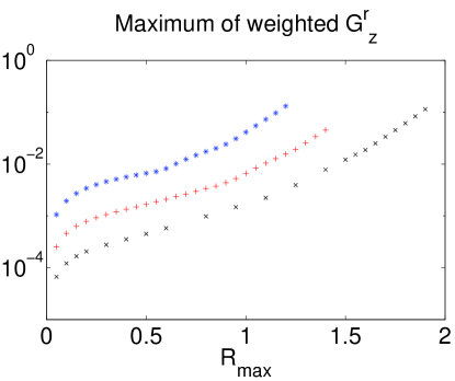
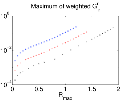
Figure 13: Plots showing the peak value of the two measure weighted constraints, $G^{r}_{~{}z}$ and $G^{r}_{~{}r}$, in the $r=0$, $z=L$ corner of the lattice, for three resolutions; $60*25$ (blue), $120*50$ (red) and $240*100$ (black). We see that increasing the resolution decreases the constraint violation, compatible with second order scaling. Furthermore, this shows that the large constraint violation that occurs as the convergence limit of a resolution is reached is unphysical, and is removed by simply going to a higher resolution. (Note that $B_{max}=1.9$ corresponds to $\lambda\simeq 3.9$)

References

- [1] H. Weyl: Ann. Phys. (Leipzig) 54 (1917) 117.
- [2] R. Emparan and H. Reall: Generalized Weyl solutions. Phys. Rev. D65 (2002) 084025, hep-th/0110258.
- [3] R. Emparan and H. Reall: A rotating black ring in five dimensions. Phys. Rev. Lett. 88 (2002) 101101, hep-th/0110260.
- [4] R. Gregory and R. Laflamme: Black strings and p-branes are unstable. Phys. Rev. Lett. 70 (1993) 2837–2840, hep-th/9301052.
- [5] R. Gregory and R. Laflamme: Hypercylindrical black holes. Phys. Rev. D37 (1988) 305.
- [6] R. Gregory and R. Laflamme: The Instability of charged black strings and p-branes. Nucl. Phys. B428 (1994) 399–434, hep-th/9404071.
- [7] B. Kol: Topology change in general relativity and the black-hole black-string transition (2002). Preprint hep-th/0206220.
- [8] B. Kol: Explosive black hole fission and fusion in large extra dimensions (2002). Preprint hep-ph/0207037.
- [9] A. Chamblin, S. Hawking and H. Reall: Brane-world black holes. Phys. Rev. D61 (2000) 065007, hep-th/9909205.
- [10] R. Gregory: Black string instabilities in anti-de Sitter space. Class. Quant. Grav. 17 (2000) L125–132, hep-th/0004101.
- [11] T. Hirayama and G. Kang: Stable black strings in anti-de Sitter space. Phys. Rev. D64 (2001) 064010, hep-th/0104213.
- [12] G. Gibbons and S. Hartnoll: A gravitational instability in higher dimensions (2002). Preprint hep-th/0206202.
- [13] S. Gubser and I. Mitra: Instability of charged black holes in anti-de Sitter space (2000). Preprint hep-th/0009126.
- [14] S. Gubser and I. Mitra: The evolution of unstable black holes in anti-de Sitter space. JHEP 08 (2001) 018, hep-th/0011127.
- [15] V. Hubeny and M. Rangamani: Unstable horizons. JHEP 05 (2002) 027, hep-th/0202189.
- [16] H. Reall: Classical and thermodynamic stability of black branes. Phys. Rev. D64 (2001) 044005, hep-th/0104071.
- [17] J. Gregory and S. Ross: Stability and the negative mode for Schwarzschild in a finite cavity. Phys. Rev. D64 (2001) 124006, hep-th/0106220.
- [18] G. Horowitz and K. Maeda: Fate of the black string instability. Phys. Rev. Lett. 87 (2001) 131301, hep-th/0105111.
- [19] S. Gubser: On non-uniform black branes (2001). Preprint hep-th/0110193.
- [20] G. Horowitz: Playing with black strings (2002). Preprint hep-th/0205069.
- [21] M. Choptuik, L. Lehner, I. Olabarrieta, R. Petryk, F. Pretorius and H. Villegas: To appear.
- [22] L. Lehner: Numerical relativity: A review. Class. Quant. Grav. 18 (2001) R25–R86, gr-qc/0106072.
- [23] T. Harmark and N. Obers: Black holes on cylinders. JHEP 05 (2002) 032, hep-th/0204047.
- [24] G. Horowitz and K. Maeda: Inhomogeneous near-extremal black branes. Phys. Rev. D65 (2002) 104028, hep-th/0201241.
- [25] P. De Smet: Black holes on cylinders are not algebraically special (2002). Preprint hep-th/0206106.
- [26] T. Wiseman: Relativistic stars in Randall-Sundrum gravity. Phys. Rev. D65 (2002) 124007, hep-th/0111057.
- [27] L. Randall and R. Sundrum: A large mass hierarchy from a small extra dimension. Phys. Rev. Lett. 83 (1999) 3370–3373, hep-ph/9905221.
- [28] L. Randall and R. Sundrum: An alternative to compactification. Phys. Rev. Lett. 83 (1999) 4690–4693, hep-th/9906064.
- [29] T. Wiseman: http://www.damtp.cam.ac.uk/user/tajw2.
- [30] R. Myers: Higher dimensional black holes in compactified space-times. Phys. Rev. D35 (1987) 455.
- [31] R. Gregory and A. Padilla: Nested braneworlds and strong brane gravity. Phys. Rev. D65 (2002) 084013, hep-th/0104262.
- [32] R. Emparan, G. Horowitz and R. Myers: Exact description of black holes on branes. JHEP 01 (2000) 007, hep-th/9911043.
- [33] A. Chamblin, H. Reall, H. Shinkai and T. Shiromizu: Charged brane-world black holes. Phys. Rev. D63 (2001) 064015, hep-th/0008177.
- [34] R. Casadio and L. Mazzacurati: Bulk shape of brane-world black holes (2002). Preprint hep-th/0205129.
- [35] T. Wiseman: Strong brane gravity and the radion at low energies. Class. Quant. Grav. 19 (2002) 3083–3106, hep-th/0201127.
- [36] S. Kanno and J. Soda: Radion and holographic brane gravity (2002). Preprint hep-th/0207029.
- [37] R. Arnowitt, S. Deser and C. Misner: The dynamics of general relativity. Gravitation: An introduction to current research, edited by L. Witten (John Wiley, New York) (1962).
- [38] W. Press, S. Teukolsky, W. Vetterling and B. Flannery: Numerical recipes. Cambridge University Press.
- [39] B. Kol: Speculative generalization of black hole uniqueness to higher dimensions (2002). Preprint hep-th/0208056.
- [40] T. Tanaka: Classical black hole evaporation in Randall-Sundrum infinite braneworld (2002). Preprint hep-th/0203082.
- [41] R. Emparan, A. Fabbri and N. Kaloper: Quantum black holes as holograms in AdS braneworlds (2002). Preprint hep-th/0206155.
- [42] S. Hawking and G. Horowitz: The gravitational Hamiltonian, action, entropy and surface terms. Class. Quant. Grav. 13 (1996) 1487–1498, gr-qc/9501014.