Abstract

By exploiting a correspondence between Random Regge triangulations (i.e., Regge triangulations with variable connectivity) and punctured Riemann surfaces, we propose a possible characterization of the $SU(2)$ Wess-Zumino-Witten model on a triangulated surface of genus $g$. Techniques of boundary CFT are used for the analysis of the quantum amplitudes of the model at level $\kappa=1$. These techniques provide a non-trivial algebra of boundary insertion operators governing a brane-like interaction between simplicial curvature and WZW fields. Through such a mechanism, we explicitly characterize the partition function of the model in terms of the metric geometry of the triangulation, and of the $6j$ symbols of the quantum group $SU(2)_{Q}$, at $Q=e^{\sqrt{-1}\pi/3}$. We briefly comment on the connection with bulk Chern-Simons theory.

PACS: 04.60.Nc, 11.25.Hf.

Keywords: Dynamical triangulations theory, Boundary conformal field theory.

1 Introduction

According to the holographic principle, in any theory combining quantum mechanics with gravity the foundamental degrees of freedom are arranged in such a way to give a quite peculiar upper bound to the total number of independent quantum states. The latter are indeed supposed to grow exponentially with the surface area rather than with the volume of the system. The standard argument motivating such a view of the holographic principle relies on the finitess of the black hole entropy: the number of ”bits” of information that can be localized on the black hole horizon is finite and determined by the area of the horizon. This led ’t Hooft [1] to conjecture the emergence of discrete structures describing the degrees of freedom localized on the black hole horizon and an explicit and significant example in the context of the S-matrix Ansatz program has been given in [2]. More recently [3] the same author has extended these considerations much beyond the physics of quantum black holes, speculating that a sort of ”discrete” quantum theory is at the heart of the Planckian scale scenario, resembling a sort of cellular automaton.

In view of these considerations, simplicial quantum gravity [4] seems a rather natural framework within which discuss the holographic principle. And, in this connection, some of us have recently proposed [5] a holographic projection mechanism for a Ponzano-Regge model living on a 3-manifold with non-empty fluctuating boundary. Related and very interesting scenarios have been proposed also in [6]. Although such a discrete philosophy seems appealing, it must be said that [5] fails short in bringing water to the mills of the holographic principle since it is difficult to pinpoint the exact nature of the (simplicial) boundary theory which holographically characterizes the bulk Ponzano-Regge gravity. It is natural to conjecture that such a boundary theory should be related with a $SU(2)$ WZW model, but the long-standing problem of the lack of a suitable characterization of WZW models on metric triangulated surfaces makes any such an identification difficult to carry out explicitly. As a matter of fact, quite indipendently from any holographic issue, the formulation of WZW theory on a discretized manifold is a subject of considerable interest in itself, and its potential field of applications is vast, ranging from the classical connection with Chern-Simons theory and quantum groups, to moduli space geometry and modern string theory dualities. It must be stressed that there have been many attempts to characterize discrete WZW models starting from discretized version of Chern-Simons theory (see e.g. [7]). Rather than providing yet another version of such a story, here we do not start with Chern-Simons theory and work explicitly toward defining a procedure for characterizing directly WZW models on triangulated surfaces.

Many of the difficulties in blending WZW theory and Regge calculus (in any of its variants) stem from the usual technical problems in putting the dynamics of $G$-valued fields ($G$ a compact Lie group) on a (randomly) triangulated space: difficulties ranging from the correct simplicial definitions of the domain of the $G$-fields, to their non-trivial dependence from the topology of the underlying triangulation. A proper formulation becomes much more feasible if one could introduce a description of the geometry of randomly triangulated surface which is more analytic in spirit, not relying exclusively on the minutiae of the combinatorics of simplicial methods. Precisely with these latter motivation in mind some of us have recently looked [8], [9] into the analytical aspects of the geometry of (random) Regge triangulated surfaces. The resulting theory turns out to be very rich and structured since it naturally maps triangulated surfaces into pointed Riemann surfaces, and thus appears as a suitable framework for providing a viable formalism for characterizing WZW models on Regge (and dynamically) triangulated surfaces.

The main goal of this note is to apply the result of [9] to the introduction of $SU(2)$ WZW theory on metrically triangulated surfaces. In order to keep the paper to a reasonable size and in order to coming quickly to grips with the main points involved we limit ourselves here to the analysis of the model in its non-trivial geometrical aspects, (some partial results in this connection have been announced in [10]), and to an explicit characterization of the partition function of the theory at level $\kappa=1$. Such a partition function has an interesting structure which directly involves the $6j$-symbols of the quantum group $SU(2)_{Q}$ at $Q=e^{\sqrt{-1}\pi/3}$, and depends in a non-trivial way from the metric geometry of the underlying triangulated surface. In its general features, it is not dissimilar from the (holographic) boundary partition function discussed in [5], and owing to the explicit presence of the $SU(2)_{Q}$ $6j$-symbols one naturally expects for a rather direct connection with a bulk Turaev-Viro model. Such a connection would frame in a nice combinatorial setup the known correspondence between the space of conformal blocks of the WZW model and the space of physical states of the bulk Chern-Simons theory. We do not reach such an objective here, nonetheless we pinpoint a few important elements which indicate that such a correspondence does indeed extend to our combinatorial framework. A detailed discussion of the relation with Chern-Simons theory, which puts to the fore the particular holographic issues that motivated us, will be presented elsewhere.

Even if still incomplete in fulfilling its original holographic motivations, our analysis of the WZW model on a triangulated surface exploits a few intermediate constructions and ideas that by themselves can be of intrinsic interest, since they put the whole subject in a wider perspective. In particular, the uniformization of a metric triangulated surface by means of a Riemann surface with (finite) cylindrical ends allows for an efficient use of boundary conformal field theory, and provides a rather direct connection with brane theory (here on group manifolds). We exploit such an interpretation for providing a description of the coupling mechanism between the (quantum) dynamics of the WZW fields and simplicial curvature. Roughly speaking, from the point of view of the dynamics of the WZW fields, (simplicial) curvature is seen as an exchange of closed strings between 2-branes in the group manifold. The interaction between the various closed string channels, (corresponding to the distinct curvature carrying vertices), is mediated by the operator product expansion between boundary insertion operators which are naturally associated with the metric ribbon graph defined by the 1-skeleton of the underlying triangulation. Note that, by uniformizing a random Regge triangulation with a (flat) Riemann surface with cylindrical ends, we are trading simplicial curvature for a modular parameter (the modulus of each cylindrical end turns out to be proportional to the conical angle of the corresponding vertex), and one is not plugging curvature by hands in the theory. Roughly speaking, gravity is indirectly read through the structure of the interaction between WZW fields and the modular parameters governing the closed string propagation between group branes. (Alternatively, by Cardy duality, one can use an open string picture, with the cylindrical ends seen as closed loops diagrams of open strings with boundary points constrained to the group branes. In such a framework, the coupling with simplicial gravity can be seen as a Casimir like effect). These remarks suggest that simplicial methods have a role which is more foundational than usually assumed and that they may provide a useful and reliable technique in a brane scenario.

Let us briefly summarize the content of the paper. In section 2, after providing a few basic definitions, we recall the main results of [8] and [9] which feature prominently in the construction of the WZW model on a Regge (and/or dynamical) triangulation. Here we introduce the correspondence between metric triangulated surfaces and the uniformization of a Riemann surface with cylindrical ends which is at the heart of the paper.

In section 3 we discuss how we can naturally associate a $SU(2)$ WZW model to a (random) Regge triangulation. The basic idea is to formulate WZW on the Riemann surface associated with the triangulation. In this way one can exploit all the known techniques of standard (i.e., continuum) WZW theory, and at the same time keep track of the relevant discrete aspects of the geometry of the original triangulation. A delicate point here concerns the imposition of suitable boundary conditions for the WZW fields at the cylindrical ends of the surface (the request for such boundary conditions cannot be avoided: it is a reflection of the fact that we cannot arbitrarily specify a WZW field at a conical vertex, there are monodromies to be respected). Our choice of boundary conditions is based on the remarkable analysis of the boundary value theory of the WZW model due to K. Gawȩdzki [11]. We discuss in detail all the steps needed for a proper characterization of the Zumino-Witten terms. As is known, this requires keeping track of the ambiguities in dealing with the extension of WZW maps to a three-dimensional bulk manifold bounded by the given Riemann surface. Such analysis naturally provides the proper set-up for moving to the quantum theory.

In section 4 we discuss the quantum amplitude of the model at level $\kappa=1$, (the reason for such a restriction are basically representation theoretic). By analysing a natural factorization property of the WZW partition function on triangulated surface, we show how to exploit the results of [12] in order to characterize the quantum amplitudes on each cylindrical end. We then discuss how such amplitudes interact along the ribbon graph associated with the underlying metrical triangulation. This step requires a rather detailed analysis of boundary insertion operators and of their operator product expansions along the vertices and edges of the ribbon graph. Here we are basically dealing with an application of well-known sewing constraint techniques in boundary CFT, (relevant references for this part of the paper are [13],[14],[15]). In particular, we exploit the connection between the OPE coefficient of such boundary operators and the $6j$-symbols of the quantum group $SU(2)_{Q}$, [15],[16]. Finally, by factorizing a correlator of boundary insertion operators along the channels associated with the edge of the ribbon graph, we evaluate the partition function of the theory at level $\kappa=1$. We conclude the paper with a a few remarks on the nature of such partition function indicating some of the features which corroborate its natural connection with a (discretized) bulk Chern-Simons theory.

2 Uniformizing triangulated surfaces

Let $M$ denote a closed 2-dimensional oriented manifold of genus $g$. A (generalized) random Regge triangulation [8] of $M$ is a homeomorphism $|T_{l}|\rightarrow{M}$ where $T$ denote a $2$-dimensional semi-simplicial complex with underlying polyhedron $|T|$ and where each edge $\sigma^{1}(h,j)$ of $T$ is realized by a rectilinear simplex of variable length $l(h,j)$. Note that since $T$ is semi-simplicial, the star of a vertex $\sigma^{0}(j)\in T$ (the union of all triangles of which $\sigma^{0}(j)$ is a face) may contain just one triangle. Note also that the connectivity of $T$ is not a priori fixed as in the case of standard Regge triangulations (see [8] for details). In such a setting a (semi-simplicial) dynamical triangulation $|T_{l=a}|\rightarrow{M}$ is a particular case [17] of a random Regge PL-manifold realized by rectilinear and equilateral simplices of a fixed edge-length $l(h,j)=$ $a$, for all the $N_{1}(T)$ edges, where $N_{i}(T)\in\mathbb{N}$ is the number of $i$-dimensional subsimplices $\sigma^{i}(...)$ of $T$. Consider the (first) barycentric subdivision $T^{(1)}$ of $|T_{l}|\rightarrow{M}$. The closed stars, in such a subdivision, of the vertices of the original triangulation $|T_{l}|\rightarrow{M}$ form a collection of $2$-cells $\{\rho^{2}(i)\}_{i=1}^{N_{0}(T)}$ characterizing the conical Regge polytope $|P_{T_{l}}|\rightarrow{M}$ (and its rigid equilateral specialization $|P_{T_{a}}|\rightarrow{M}$) barycentrically dual to $|T_{l}|\rightarrow{M}$. The adjective conical emphasizes that here we are considering a geometrical presentation $|P_{T_{l}}|\rightarrow{M}$ of $P$ where the $2$-cells $\{\rho^{2}(i)\}_{i=1}^{N_{0}(T)}$ retain the conical geometry induced on the barycentric subdivision by the original metric structure of $|T_{l}|\rightarrow{M}$. This latter is locally Euclidean everywhere except at the vertices $\sigma^{0}$, (the bones), where the sum of the dihedral angles, $\theta(\sigma^{2})$, of the incident triangles $\sigma^{2}$’s is in excess (negative curvature) or in defect (positive curvature) with respect to the $2\pi$ flatness constraint. The corresponding deficit angle $\varepsilon$ is defined by $\varepsilon=2\pi-\sum_{\sigma^{2}}\theta(\sigma^{2})$, where the summation is extended to all $2$ -dimensional simplices incident on the given bone $\sigma^{0}$. In the case of dynamical triangulations [17] the deficit angles are generated by the numbers $\#\{\sigma^{2}(h,j,k)\bot\sigma^{0}(k)\}$ of triangles incident on the $N_{0}(T)$ vertices, the curvature assignments, $\{q(k)\}_{k=1}^{N_{0}(T)}\in\mathbb{N}^{N_{0}(T)}$, in terms of which we can write $\varepsilon(k)=2\pi-\pi q(k)/3$.

It is worthwhile stressing that the natural automorphism group $Aut(P_{l})$ of $|P_{T_{l}}|\rightarrow{M}$, (i.e., the set of bijective maps preserving the incidence relations defining the polytopal structure), is the automorphism group of the edge refinement $\Gamma$ (see [18]) of the $1$-skeleton of the conical Regge polytope $|P_{T_{l}}|\rightarrow{M}$. Such a $\Gamma$ is the $3$-valent graph

$$\Gamma=\left(\{\rho^{0}(h,j,k)\}\bigsqcup^{N_{1}(T)}\{W(h,j)\},\{\rho^{1}(h,j)^{+}\}\bigsqcup^{N_{1}(T)}\{\rho^{1}(h,j)^{-}\}\right).$$ (1)

where the vertex set $\{\rho^{0}(h,j,k)\}^{N_{2}(T)}$ is identified with the barycenters of the triangles $\{\sigma^{o}(h,j,k)\}^{N_{2}(T)}\in|T_{l}|\rightarrow M$, whereas each edge $\rho^{1}(h,j)\in\{\rho^{1}(h,j)\}^{N_{1}(T)}$ is generated by two half-edges $\rho^{1}(h,j)^{+}$ and $\rho^{1}(h,j)^{-}$ joined through the barycenters $\{W(h,j)\}^{N_{1}(T)}$ of the edges $\{\sigma^{1}(h,j)\}$ belonging to the original triangulation $|T_{l}|\rightarrow M$. The (counterclockwise) orientation in the $2$-cells $\{\rho^{2}(k)\}$ of $|P_{T_{l}}|\rightarrow{M}$ gives rise to a cyclic ordering on the set of half-edges $\{\rho^{1}(h,j)^{\pm}\}^{N_{1}(T)}$ incident on the vertices $\{\rho^{0}(h,j,k)\}^{N_{2}(T)}$. According to these remarks, the (edge-refinement of the) $1$-skeleton of $|P_{T_{l}}|\rightarrow{M}$ is a ribbon (or fat) graph [18], viz., a graph $\Gamma$ together with a cyclic ordering on the set of half-edges incident to each vertex of $\Gamma$. Conversely, any ribbon graph $\Gamma$ characterizes an oriented surface $M(\Gamma)$ with boundary possessing $\Gamma$ as a spine, ( i.e., the inclusion $\Gamma\hookrightarrow M(\Gamma)$ is a homotopy equivalence). In this way (the edge-refinement of) the $1$-skeleton of a generalized conical Regge polytope $|P_{T_{l}}|\rightarrow{M}$ is in a one-to-one correspondence with trivalent metric ribbon graphs.

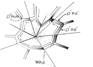
Figure 1: The ribbon graph associated with the barycentrically dual polytope.

As we have shown in [8], [9] it is possible to naturally relax, (in the technical sense of the theory of geometrical structures [19]), the singular Euclidean structure associated with the conical polytope $|P_{T_{l}}|\rightarrow{M}$ to a complex structure $((M;N_{0}),\mathcal{C})$. Such a relaxing is defined by exploiting [18] the ribbon graph $\Gamma$ (see (1)), and for later use we need to recall some of the results of [9] by adopting a notation more suitable to our purposes. Let $\rho^{2}(h)$, $\rho^{2}(j)$, and $\rho^{2}(k)$ respectively be the two-cells $\in|P_{T_{l}}|\rightarrow{M}$ barycentrically dual to the vertices $\sigma^{0}(h)$, $\sigma^{0}(j)$, and $\sigma^{0}(k)$ of a triangle $\sigma^{2}(h,j,k)\in|T_{l}|\rightarrow M$. Let us denote by $\rho^{1}(h,j)$ and $\rho^{1}(j,h)$, respectively, the oriented edges of $\rho^{2}(h)$ and $\rho^{2}(j)$ defined by

$$\rho^{1}(h,j)\bigsqcup\rho^{1}(j,h)\doteq\partial\rho^{2}(h)\bigcap_{\Gamma}\partial\rho^{2}(j),$$ (2)

i.e., the portion of the oriented boundary of  $\Gamma$ intercepted by the two adjacent oriented cells $\rho^{2}(h)$ and $\rho^{2}(j)$  (thus $\rho^{1}(h,j)\in\rho^{2}(h)$ and $\ \rho^{1}(j,h)\in\rho^{2}(j)$ carry opposite orientations). Similarly, we shall denote by $\rho^{0}(h,j,k)$ the $3$-valent, cyclically ordered, vertex of $\Gamma$ defined by

$$\rho^{0}(h,j,k)\doteq\partial\rho^{2}(h)\bigcap_{\Gamma}\partial\rho^{2}(j)\bigcap_{\Gamma}\partial\rho^{2}(k).$$ (3)

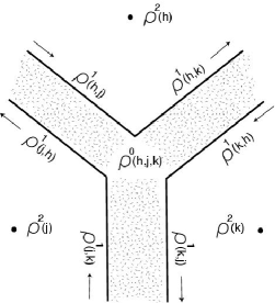
Figure 2: The 2-cells,the oriented edges, and the oriented vertices of the conical dual polytope.

To the edge $\rho^{1}(h,j)$ of $\rho^{2}(h)$ we associate [18] a complex coordinate $z(h,j)$ defined in the strip

$$U_{\rho^{1}(h,j)}\doteq\{z(h,j)\in\mathbb{C}|0<\mathop{\mathrm{R}e}z(h,j)<L(h,j)\},$$ (4)

$L(h,j)$ being the length of the edge considered. The coordinate $w(h,j,k)$, corresponding to the $3$-valent vertex $\rho^{0}(h,j,k)\in\rho^{2}(h)$, is defined in the open set

$$U_{\rho^{0}(h,j,k)}\doteq\{w(h,j,k)\in\mathbb{C}|\;|w(h,j,k)|<\delta,\;w(h,j,k)[\rho^{0}(h,j,k)]=0\},$$ (5)

where $\delta>0$ is a suitably small constant. Finally, the generic two-cell $\rho^{2}(k)$ is parametrized in the unit disk

$$U_{\rho^{2}(k)}\doteq\{\zeta(k)\in\mathbb{C}|\;|\zeta(k)|<1,\;\zeta(k)[\sigma^{0}(k)]=0\},$$ (6)

where $\sigma^{0}(k)$ is the vertex $\in|T_{l}|\rightarrow M$ corresponding to the given two-cell.

We define the complex structure $((M;N_{0}),\mathcal{C})$ by coherently gluing, along the pattern associated with the ribbon graph $\Gamma$, the local coordinate neighborhoods $\{U_{\rho^{0}(h,j,k)}\}_{(h,j,k)}^{N_{2}(T)}$, $\{U_{\rho^{1}(h,j)}\}_{(h,j)}^{N_{1}(T)}$, and $\{U_{\rho^{2}(k)}\}_{(k)}^{N_{0}(T)}$. Explicitly, (see [18] for an elegant exposition of the general theory and [8], [9] for the application to simplicial gravity), let $\{U_{\rho^{1}(h,j)}\}$, $\{U_{\rho^{1}(j,k)}\}$, $\{U_{\rho^{1}(k,h)}\}\$ be the three generic open strips associated with the three cyclically oriented edges $\rho^{1}(h,j)$, $\rho^{1}(j,k)$, $\rho^{1}(k,h)$ incident on the vertex $\rho^{0}(h,j,k)$. Then the corresponding coordinates $z(h,j)$, $z(j,k)$, and $z(k,h)$ are related to $w(h,j,k)$ by the transition functions

$$w(h,j,k)=\left\{\begin{tabular}[]{l}$z(h,j)^{\frac{2}{3}},$\\ $e^{\frac{2\pi}{3}\sqrt{-1}}z(j,k)^{\frac{2}{3}},$\\ $e^{{}^{\frac{4\pi}{3}\sqrt{-1}}}z(k,h)^{\frac{2}{3}},$\end{tabular}\right..$$ (7)

Similarly, if $\{U_{\rho^{1}(h,j_{\beta})}\}$, $\beta=1,2,...,q(k)$ are the open strips associated with the $q(k)$ (oriented) edges $\{\rho^{1}(h,j_{\beta})\}$ boundary of the generic polygonal cell $\rho^{2}(h)$, then the transition functions between the corresponding coordinate $\zeta(h)$ and the $\{z(h,j_{\beta})\}$ are given by [18]

$$\zeta(h)=\exp\left(\frac{2\pi\sqrt{-1}}{L(h)}\left(\sum_{\beta=1}^{\nu-1}L(h,j_{\beta})+z(h,j_{\nu})\right)\right),\hskip 14.45377pt\nu=1,...,q(h),$$ (8)

with $\sum_{\beta=1}^{\nu-1}\cdot\doteq 0$, for $\nu=1$, and where $L(h)$ denotes the perimeter of $\partial(\rho^{2}(h))$. By iterating such a construction for each vertex $\{\rho^{0}(h,j,k)\}$ in the conical polytope $|P_{T_{l}}|\rightarrow{M}$ we get a very explicit characterization of $((M;N_{0}),\mathcal{C})$.

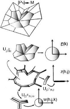
Figure 3: The complex coordinate neighborhoods associated with the dual polytope.

Such a construction has a natural converse which allows us to describe the conical Regge polytope $|P_{T_{l}}|\rightarrow{M}$ as a uniformization of $((M;N_{0}),\mathcal{C})$. In this connection, the basic observation is that, in the complex coordinates introduced above, the ribbon graph $\Gamma$ naturally corresponds to a Jenkins-Strebel quadratic differential $\phi$ with a canonical local structure which is given by [18]

$$\phi\doteq\left\{\begin{tabular}[]{l}$\phi(h)|_{\rho^{1}(h)}=dz(h)\otimes dz(h),$\\ \\ $\phi(j)|_{\rho^{0}(j)}=\frac{9}{4}w(j)dw(j)\otimes dw(j),$\\ \\ $\phi(k)|_{\rho^{2}(k)}=-\frac{\left[L(k)\right]^{2}}{4\pi^{2}\zeta^{2}(k)}d\zeta(k)\otimes d\zeta(k),$\end{tabular}\right.$$ (9)

where $L(k)$ denotes the perimeter of $\partial(\rho^{2}(k))$, and where $\rho^{0}(h,j,k)$, $\rho^{1}(h,j)$, $\rho^{2}(k)$ run over the set of vertices, edges, and $2$-cells of $|P_{l}|\rightarrow M$. If we denote by

$$\Delta_{k}^{\ast}\doteq\{\zeta(k)\in\mathbb{C}|\;0<|\zeta(k)|<1\},$$ (10)

the punctured disk $\Delta_{k}^{\ast}\subset U_{\rho^{2}(k)}$, then for each given deficit angle $\varepsilon(k)=2\pi-\theta(k)$ we can introduce on each $\Delta_{k}^{\ast}$ the conical metric

$$ds_{(k)}^{2} \doteq \frac{\left[L(k)\right]^{2}}{4\pi^{2}}\left|\zeta(k)\right|^{-2\left(\frac{\varepsilon(k)}{2\pi}\right)}\left|d\zeta(k)\right|^{2}=$$

$$= \left|\zeta(k)\right|^{2\left(\frac{\theta(k)}{2\pi}\right)}|\phi(k)_{\rho^{2}(k)}|,$$

where

$$|\phi(k)_{\rho^{2}(k)}|=\frac{\left[L(k)\right]^{2}}{4\pi^{2}|\zeta(k)|^{2}}|d\zeta(k)|^{2}.$$ (12)

is the standard cylindrical metric associated with the quadratic differential $\phi(k)_{\rho^{2}(k)}$.

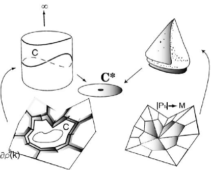
Figure 4: The cylindrical and the conical metric over a polytopal cell.

In order to describe the geometry of the uniformization of $((M;N_{0}),\mathcal{C}))$ defined by $\{ds_{(k)}^{2}\}$, let us consider the image in $((M;N_{0}),\mathcal{C}))$ of the generic triangle $\sigma^{2}(h,j,k)\in|T_{l}|\rightarrow M$ of sides $\sigma^{1}(h,j)$, $\sigma^{1}(j,k)$, and $\sigma^{1}(k,h)$. Similarly, let $W(h,j)$, $W(j,k)$, and $W(k,h)$ be the images of the respective barycenters, (see (1)). Denote by $\widehat{L}(k)=|W(h,j)\rho^{0}(h,j,k)|$, $\widehat{L}(h)=|W(j,k)\rho^{0}(h,j,k)|$, and $\widehat{L}(j)=|W(k,h)\rho^{0}(h,j,k)|$, the lengths, in the metric $\{ds_{(k)}^{2}\}$, of the half-edges connecting the (image of the) vertex $\rho^{0}(h,j,k)$ of the ribbon graph $\Gamma$ with $W(h,j)$, $W(j,k)$, and $W(k,h)$. Likewise, let us denote by $l(\bullet,\bullet)$ the length of the corresponding side $\sigma^{1}(\bullet,\bullet)$ of the triangle. A direct computation involving the geometry of the medians of $\sigma^{2}(h,j,k)$ provides

$$\begin{tabular}[]{ccc}$\widehat{L}^{2}(j)$&$=$&$\frac{1}{18}l^{2}(j,k)+\frac{1}{18}l^{2}(h,j)-\frac{1}{36}l^{2}(k,h)$\\ $\widehat{L}^{2}(k)$&$=$&$\frac{1}{18}l^{2}(k,h)+\frac{1}{18}l^{2}(j,k)-\frac{1}{36}l^{2}(h,j)$\\ $\widehat{L}^{2}(h)$&$=$&$\frac{1}{18}l^{2}(h,j)+\frac{1}{18}l^{2}(k,h)-\frac{1}{36}l^{2}(j,k)$\\ &&\\ $l^{2}(k,h)$&$=$&$8\widehat{L}^{2}(h)+8\widehat{L}^{2}(k)-4\widehat{L}^{2}(j)$\\ $l^{2}(h,j)$&$=$&$8\widehat{L}^{2}(j)+8\widehat{L}^{2}(h)-4\widehat{L}^{2}(k)$\\ $l^{2}(j,k)$&$=$&$8\widehat{L}^{2}(k)+8\widehat{L}^{2}(j)-4\widehat{L}^{2}(h)$\end{tabular},$$ (13)

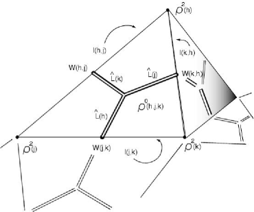
Figure 5: The relation between the edge-lengths of the conical polytope and the edge-lenghts of the triangulation.

which allows to recover, as the indices $(h,j,k)$ vary, the metric geometry of $|P_{T_{l}}|\rightarrow{M}$ and of its dual triangulation $|T_{l}|\rightarrow M$, from $((M;N_{0}),\mathcal{C});\{ds_{(k)}^{2}\})$. In this sense, the stiffening [19] of $((M;N_{0}),\mathcal{C})$ defined by the punctured Riemann surface

$$((M;N_{0}),\mathcal{C});\{ds_{(k)}^{2}\})=$$ (14)

$$=\bigcup_{\{\rho^{0}(h,j,k)\}}^{N_{2}(T)}U_{\rho^{0}(h,j,k)}\bigcup_{\{\rho^{1}(h,j)\}}^{N_{1}(T)}U_{\rho^{1}(h,j)}\bigcup_{\{\rho^{2}(k)\}}^{N_{0}(T)}(\Delta_{k}^{\ast},ds_{(k)}^{2}),$$

is the uniformization of $((M;N_{0}),\mathcal{C})$ associated [9] with the conical Regge polytope $|P_{l}|\rightarrow M$.

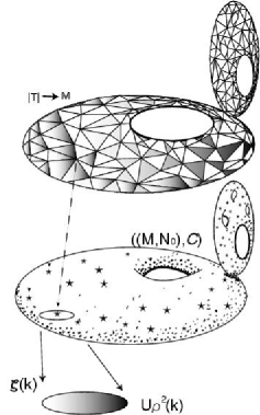
Figure 6: The decorated punctured Riemann surface associated with a random Regge triangulation.

Although the correspondence between conical Regge polytopes and the above punctured Riemann surface is rather natural there is yet another uniformization representation of $|P_{l}|\rightarrow M$ which is of relevance in discussing conformal field theory on a given $|P_{l}|\rightarrow M$. The point is that the analysis of a CFT on a singular surface such as $|P_{l}|\rightarrow M$ calls for the imposition of suitable boundary conditions in order to take into account the conical singularities of the underlying Riemann surface $((M;N_{0}),\mathcal{C},ds^{2}_{(k)})$. This is a rather delicate issue since conical metrics give rise to difficult technical problems in discussing the glueing properties of the resulting conformal fields. In boundary conformal field theory, problems of this sort are taken care of (see e.g.[[11]]) by (tacitly) assuming that a neighborhood of the possible boundaries is endowed with a cylindrical metric. In our setting such a prescription naturally calls into play the metric associated with the quadratic differential $\phi$, and requires that we regularize into finite cylindrical ends the cones $(\Delta_{k}^{\ast},ds_{(k)}^{2})$.   Such a regularization is realized by noticing that if we introduce the annulus

$$\Delta_{\theta(k)}^{\ast}\doteq\left\{\zeta(k)\in\mathbb{C}|e^{-\frac{2\pi}{\theta(k)}}\leq|\zeta(k)|\leq 1\right\}\subset\overline{U_{\rho^{2}(k)}},$$ (15)

then the surface with boundary

$$M_{\partial}\doteq((M_{\partial};N_{0}),\mathcal{C})=\bigcup U_{\rho^{0}(j)}\bigcup U_{\rho^{1}(h)}\bigcup(\Delta_{\theta(k)}^{\ast},\phi(k))$$ (16)

defines the blowing up of the conical geometry of  $((M;N_{0}),\mathcal{C},ds_{(k)}^{2})$ along the ribbon graph $\Gamma$.

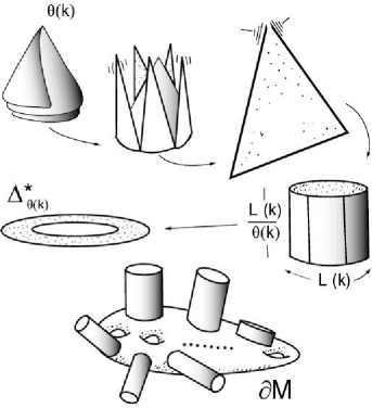
Figure 7: Blowing up the conical geometry of the polytope into finite cylindrical ends generates a uniformized Riemann surface with cylindrical boundaries.

The metrical geometry of  $(\Delta_{\theta(k)}^{\ast},\phi(k))$ is that of a flat cylinder with a circumference of length given by $L(k)$ and heigth given by $L(k)/\theta(k)$, (this latter being the slant radius of the generalized Euclidean cone $(\Delta_{k}^{\ast},ds_{(k)}^{2})$ of base circumference $L(k)$ and vertex conical angle $\theta(k)$).We also have

$$\partial M_{\partial} = \bigsqcup_{k=1}^{N_{0}}S_{\theta(k)}^{(+)},$$ (17)

$$\partial\Gamma = \bigsqcup_{k=1}^{N_{0}}S_{\theta(k)}^{(-)}$$

where the circles

$$S_{\theta(k)}^{(+)} \doteq \left\{\zeta(k)\in\mathbb{C}||\zeta(k)|=e^{-\frac{2\pi}{\theta(k)}}\right\},$$ (18)

$$S_{\theta(k)}^{(-)} \doteq \left\{\zeta(k)\in\mathbb{C}||\zeta(k)|=1\right\}$$

respectively denote the inner and the outer boundary of the annulus $\Delta_{\theta(k)}^{\ast}$. Note that by collapsing $S_{\theta(k)}^{(+)}$ to a point we get back the original cones $(\Delta_{k}^{\ast},ds_{(k)}^{2})$. Thus, the surface with boundary $M_{\partial}$ naturally corresponds to the ribbon graph $\Gamma$ associated with the 1-skeleton $K_{1}(|P_{T_{l}}|\rightarrow{M})$ of the polytope $|P_{T_{l}}|\rightarrow{M}$, decorated with the finite cylinders $\{\Delta_{\theta(k)}^{\ast},|\phi(k)|\}$. In such a framework the conical angles $\{\theta(k)=2\pi-\varepsilon(k)\}$ appears as (reciprocal of the) moduli $m_{k}$ of the annuli $\{\Delta_{\theta(k)}^{\ast}\}$,

$$m(k)=\frac{1}{2\pi}\ln\frac{1}{e^{-\frac{2\pi}{\theta(k)}}}=\frac{1}{\theta(k)}$$ (19)

(recall that the modulus of an annulus $r_{0}<|\zeta|<r_{1}$ is defined by $\frac{1}{2\pi}\ln\frac{r_{1}}{r_{0}}$). According to these remarks we can equivalently represent the conical Regge polytope $|P_{T_{l}}|\rightarrow{M}$ with the uniformization $((M;N_{0}),\mathcal{C});\{ds_{(k)}^{2}\})$ or with its blowed up version $M_{\partial}$.

3 The WZW model on a Regge polytope

Let $G$ be a connected and simply connected Lie group. In order to make things simpler we shall limit our discussion to the case $G=SU(2)$, this being the case of more direct interest to us. Recall [11] that the complete action of the Wess-Zumino-Witten model on a closed Riemann surface $M$ of genus $g$ is provided by

$$S^{WZW}(h)=\frac{\kappa}{4\pi\sqrt{-1}}\int_{M}tr\left(h^{-1}\partial h\right)\left(h^{-1}\overline{\partial}h\right)+S^{WZ}(h),$$ (20)

where $h:M\rightarrow SU(2)$ denotes a $SU(2)$-valued field on $M$, $\kappa$ is a positive constant (the level of the model), $tr(\cdot)$ is the Killing form on the Lie algebra (normalized so that the root has length $\sqrt{2}$) and $S^{WZ}(h)$ is the topological Wess-Zumino term needed [20] in order to restore conformal invariance of the theory at the quantum level. Explicitly, $S^{WZ}(h)$ can be characterized by extending the field $h:M\rightarrow SU(2)$ to maps $\widetilde{h}:V_{M}\rightarrow SU(2)$ where $V_{M}$ is a three-manifold with boundary such that $\partial V_{M}=M$, and set

$$S^{WZ}(h)=\frac{\kappa}{4\pi\sqrt{-1}}\int_{V_{M}}\widetilde{h}^{\ast}\chi_{SU(2)},$$ (21)

where $\widetilde{h}^{\ast}\chi_{SU(2)}$ denotes the pull-back to $V_{M}$ of the canonical 3-form on $SU(2)$

$$\chi_{SU(2)}\doteq\frac{1}{3}tr\left(h^{-1}dh\right)\wedge\left(h^{-1}dh\right)\wedge\left(h^{-1}dh\right),$$ (22)

(recall that for $SU(2)$, $\chi_{SU(2)}$ reduces to $4\mu_{S^{3}}$, where $\mu_{S^{3}}$ is the volume form on the unit 3-sphere $S^{3}$). As is well known, $S^{WZ}(h)$ so defined depends on the extension $\widetilde{h}$ , the ambiguity being parametrized by the period of the form $\chi_{SU(2)}$ over the integer homology $H_{3}(SU(2))$. Demanding that the Feynman amplitude $e^{-S^{WZW}(h)}$ is well defined requires that the level $\kappa$ is an integer.

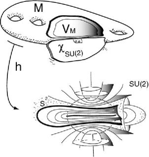
Figure 8: The geometrical set up for the WZW model. The surface M opens up to show the associated handlebody. The group SU(2) is here shown as the 3-sphere foliated into (squashed) 2-spheres.

3.1 Polytopes and the WZW model with boundaries

From the results discussed in section 2, it follows that a natural strategy for introducing the WZW model on the Regge polytope $|P_{T_{l}}|\rightarrow{\ M}$ is to consider maps $h:M_{\partial}\rightarrow SU(2)$ on the associated surface with cylindrical boundaries $M_{\partial}\doteq((M_{\partial};N_{0}),\mathcal{C})$. Such maps $h$ should satisfy suitable boundary conditions on the (inner and outer) boundaries $\{S_{\theta(k)}^{(\pm)}\}$ of the annuli $\{\Delta_{\theta(k)}^{\ast}\}$, corresponding to the (given) values of the $SU(2)$ field on the boundaries of the cells of $|P_{T_{l}}|\rightarrow{\ M}$ and on their barycenters, (the field being free to fluctuate in the cells). Among all possible boundary conditions, there is a choice which is particularly simple and which allows us to reduce the study of WZW model on each given Regge polytopes to the (quantum) dynamics of WZW fields on the finite cylinders (annuli) $\{\Delta_{\theta(k)}^{\ast}\}$ decorating the ribbon graph $\Gamma$ and representing the conical cells of $|P_{T_{l}}|\rightarrow{\ M}$. Such an approach corresponds to first study the WZW model on $|P_{T_{l}}|\rightarrow{\ M}$ as a CFT. Its (quantum) states will then depend on the boundary conditions on the $SU(2)$ field $h$ on $\{S_{\theta(k)}^{(\pm)}\}$; roughly speaking such a procedure turns out to be equivalent to a prescription assigning an irreducible representation of $SU(2)$ to each barycenter of the given polytope $|P_{T_{l}}|\rightarrow{\ M}$. Such representations are parametrized by the boundary conditions which, by consistency, turn out to be necessarily quantized. They are also parametrized by elements of the geometry of $|P_{T_{l}}|\rightarrow{\ M}$, in particular by the deficit angles.

In order to carry over such a program, let us associate with each inner boundary $S_{\theta(i)}^{(+)}$ the $SU(2)$ Cartan generator

$$\Lambda_{i}\doteq\frac{\lambda(i)}{\kappa}\mathbf{\sigma}_{3}\text{, with\ }\mathbf{\sigma}_{3}=\left(\begin{array}[]{cc}1&0\\ 0&-1\end{array}\right)$$ (23)

where, for later convenience, $\lambda(i)\in\mathbb{R}$ has been normalized to the level $\kappa$,  and let

$$C_{i}^{(+)}\doteq\left\{\gamma e^{2\pi\sqrt{-1}\Lambda_{i}}\gamma^{-1}\;|\;\gamma\in SU(2)\right\}.$$ (24)

denote the (positively oriented) two-sphere $S^{2}_{\theta(i)}$ in $SU(2)$ representing the associated conjugacy class, (note that $C_{i}^{(+)}$ degenerates to a single point for the center of $SU(2)$). Such a prescription basically prevent out-flow of momentum across the boundary and has been suggested, in the framework of D-branes theory in [21], (see also [11]). Similarly, to the outer boundary $S_{\theta(i)}^{(-)}$ we associate the conjugacy class $C_{i}^{(-)}=\overline{C_{i}^{(+)}}$ describing the conjugate two-sphere $\overline{S^{2}_{\theta(i)}}$ (with opposite orientation) in $SU(2)$ associated with $S^{2}_{\theta(i)}$.  Given such data, we consider maps $h:M_{\partial}\rightarrow SU(2)$ that satisfy the fully symmetric boundary conditions [22],

$$h(S_{\theta(i)}^{(\pm)})\subset C_{i}^{(\pm)}.$$ (25)

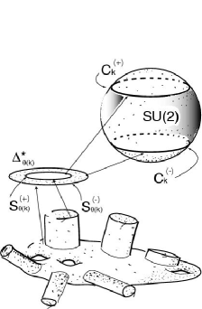
Figure 9: The geometrical setup for SU(2) boundary conditions on each $(\Delta_{\theta(k)}^{\ast},\phi(k))$ decorating the 1-skeleton of $|P_{T_{l}}|\rightarrow{M}$. For simplicity, the group SU(2) is incorrectly rendered; note that each circumference $C_{k}^{\pm}$ is actually a two-sphere, (or degenerates to a point).

Note that since $C_{i}^{(+)}$ and $C_{i}^{(-)}$ carry opposite orientations, the functions $h(S_{\theta(i)}^{(\pm)})$ are normalized to $h(S_{\theta(i)}^{(-)})h(S_{\theta(i)}^{(+)})={\mathbf{e}}$, (the identity $\in{SU(2)}$). The advantage of considering this subset of maps $h:M_{\partial}\rightarrow SU(2)$ is that when restricted to the boundary $\partial M_{\partial}$, (i.e., to the inner conjugacy classes $C_{i}^{(+)}$), the 3-form $\chi_{SU(2)}$ (22) becomes exact, and one can write

$$\left.\chi_{SU(2)}\right|_{C_{i}}=d\omega_{i},$$ (26)

where the 2-form $\omega_{i}$ is provided by

$$\omega_{i}=tr(\gamma^{-1}d\gamma)e^{2\pi\sqrt{-1}\Lambda_{i}}(\gamma^{-1}d\gamma)e^{-2\pi\sqrt{-1}\Lambda_{i}}.$$ (27)

In such a case, we can extend [11] the map $h:M_{\partial}\rightarrow SU(2)$ to a map ${\widehat{h}}:((M;N_{0}),\mathcal{C})\rightarrow SU(2)$ from the closed surface $((M;N_{0}),\mathcal{C})$ to $SU(2)$ in such a way that $\widehat{h}(\delta_{\theta(i)})\subset C_{i}^{(+)}$, where

$$\delta_{\theta(i)}\doteq\left\{\zeta(i)\in\mathbb{C}|\;|\zeta(i)|\leq e^{-\frac{2\pi}{\theta(i)}}\right\}$$ (28)

is the disk capping the cylindrical end $\{\Delta_{\theta(i)}^{\ast},|\phi(i)|\}$, (thus $\partial\delta_{\theta(i)}=S_{\theta(k)}^{(+)}$ and $\Delta_{\theta(i)}^{\ast}\cup\delta_{\theta(i)}\ \ \simeq\overline{U}_{\rho^{2}(i)}$). In this connection note that the boundary conditions $h(S_{\theta(i)}^{(+)})\subset C_{i}^{(+)}$ define elements of the loop group

$$\mathcal{L}_{(i)}SU(2)\doteq Map(S_{\theta(i)}^{(+)},SU(2))\simeq Map(S^{1},SU(2)).$$ (29)

Similarly, any other extension  $h^{\prime}_{i}=\widehat{h}_{i}g$, ($g\in SU(2)$), of $h$ over the capping disks $\delta_{\theta(i)}$, can be considered as an element of the group $Map(\delta_{\theta(i)},SU(2))$. In the same vein, we can interpret $\widetilde{h}_{i}=(\widehat{h}_{i},h_{i}^{\prime})$ as a map from the spherical double (see below) $S_{i}^{2}$ of $\delta_{\theta(i)}$ into $SU(2)$, i.e., as an element of the group $Map(S_{i}^{2},SU(2))$. It follows that each possible extension of  the boundary condition $h(S_{\theta(i)}^{(+)})$ fits into the exact sequence of groups

$$1\rightarrow Map(S_{i}^{2},SU(2))\rightarrow Map(\delta_{\theta(i)},SU(2))\rightarrow Map(S_{\theta(i)}^{(+)},SU(2))\rightarrow 1.$$ (30)

In order to discuss the properties of such extensions we can proceed as follows, (see [11] for the analysis of these and related issues in the general setting of boundary CFT).

Let us denote by $V_{M}$,  with $\partial V_{M}=((M,N_{0});\mathcal{C})$, the 3-dimensional handlebody associated with the surface $((M,N_{0});\mathcal{C})$, and corresponding to the mapping $\widehat{h}:((M,N_{0});\mathcal{C})\rightarrow SU(2)\simeq S^{3}$ thought of as an immersion in the 3-sphere. Since the conjugacy classes $C_{i}^{(+)}$ are 2-spheres and the homotopy group $\pi_{2}(SU(2))$ is trivial, we can further extend the maps $\widehat{h}$ to a smooth function $\ \widehat{H}:V_{M}\rightarrow SU(2)$, (thus, by construction  $\widehat{H}(\delta_{\theta(i)})\subset$ $C_{i}^{(+)}$). Any such an extension can be used to pull-back to the handlebody $V_{M}$ the Maurer-Cartan 3-form $\chi_{SU(2)}$ and it is natural to define the Wess-Zumino term associated with $((M,N_{0});\mathcal{C})$ according to

$$S_{|P_{T_{l}}|}^{WZ}(\widehat{h},\widehat{H})\doteq\frac{\kappa}{4\pi\sqrt{-1}}\int_{V_{M}}\widehat{H}^{\ast}\chi_{SU(2)}-\frac{\kappa}{4\pi\sqrt{-1}}\sum_{j=1}^{N_{0}}\int_{\delta_{\theta(j)}}\left.\widehat{h}\right|_{\delta_{\theta(j)}}^{\ast}\omega_{j}.$$ (31)

In general,  such a definition of  $S_{|P_{T_{l}}|}^{WZ}(\widehat{h},\widehat{H})$ depends on the particular extensions $(\widehat{h},\widehat{H})$ we are considering, and if we denote by $(h^{\prime}=\widehat{h}g,H^{\prime})$, $g\in SU(2)$, a different extension, then, by reversing the orientation of the handlebody $V_{M}$ and of the capping disks $\delta_{\theta(j)}$ over which $S_{|P_{T_{l}}|}^{WZ}(h^{\prime},H^{\prime})$ is evaluated, the difference between the resulting WZ terms can be written as

$$S_{|P_{T_{l}}|}^{WZ}(\widehat{h},\widehat{H})-S_{|P_{T_{l}}|}^{WZ}(h^{\prime},H^{\prime})=$$ (32)

$$=\frac{\kappa}{4\pi\sqrt{-1}}\left(\int_{V_{M}}\widehat{H}^{\ast}\chi_{SU(2)}+\int_{V_{M}^{(-)}}H^{\prime\ast}\chi_{SU(2)}\right)-$$

$$-\frac{\kappa}{4\pi\sqrt{-1}}\sum_{j=1}^{N_{0}}\left(\int_{\delta_{\theta(j)}}\left.\widehat{h}\right|_{\delta_{\theta(j)}}^{\ast}\omega_{j}+\int_{\delta_{\theta(j)}^{(-)}}\left.h^{\prime}\right|_{\delta_{\theta(j)}}^{\ast}\omega_{j}\right).$$

Note that

$$(V_{M},\widehat{H})\cup(V_{M}^{(-)},H^{\prime})=(\widetilde{V}_{M},\widetilde{H})$$ (33)

is the 3-manifold (ribbon graph) double of $V_{M}$  endowed with the extension $\widetilde{H}\doteq(\widehat{H},H^{\prime})$   and

$$(\delta_{\theta(j)},\widehat{h_{j}})\cup(\delta_{\theta(j)}^{(-)},h_{j}^{\prime})=(S_{j}^{2},\widetilde{h_{j}}),$$ (34)

are the 2-spheres defined by doubling the capping disks $\delta_{\theta(j)}$, decorated with the extension $\widetilde{h}_{j}\doteq(\widehat{h}_{j},h_{j}^{\prime})\in C_{j}^{(+)}$. By construction $(\widetilde{V}_{M},\widetilde{H})$ is such that $\partial(\widetilde{V}_{M},\widetilde{H})=\cup_{j=1}^{N_{0}}(S_{j}^{2},\widetilde{h_{j}})$ so that we can equivalently write (32) as

$$S_{|P_{T_{l}}|}^{WZ}(\widehat{h},\widehat{H})-S_{|P_{T_{l}}|}^{WZ}(h^{\prime},H^{\prime})=\frac{\kappa}{4\pi\sqrt{-1}}\int_{\widetilde{V}_{M}}\widetilde{H}^{\ast}\chi_{SU(2)}-$$ (35)

$$-\frac{\kappa}{4\pi\sqrt{-1}}\sum_{j=1}^{N_{0}}\int_{S_{j}^{2}}\widetilde{h}^{\ast}\omega_{j}.$$

To such an expression we add and subtract

$$\frac{\kappa}{4\pi\sqrt{-1}}\sum_{j=1}^{N_{0}}\int_{B_{j}^{3}}\widetilde{H_{j}}^{\ast}\chi_{SU(2)}$$ (36)

where $B_{j}^{3}$ are 3-balls such that $\partial B_{j}^{3}=S_{j}^{2(-)}$, (the boundary orientation is inverted so that we can glue such $B_{j}^{3}$ to the corresponding boundary components of $\widetilde{V}_{M}$), and $\widetilde{H_{j}}$ are corresponding extensions of $\widetilde{H}$ with $\widetilde{H_{j}}|_{S_{j}^{2}}=\widetilde{h}_{j}$. Since $\widetilde{V}_{M}\cup$ $B_{j}^{3}$ results in a closed 3-manifold $W^{3}$, we eventually get

$$S_{|P_{T_{l}}|}^{WZ}(\widehat{h},\widehat{H})-S_{|P_{T_{l}}|}^{WZ}(\eta)(h^{\prime},H^{\prime})=\frac{\kappa}{4\pi\sqrt{-1}}\int_{W^{3}}\widetilde{H}^{\ast}\chi_{SU(2)}-$$ (37)

$$-\frac{\kappa}{4\pi\sqrt{-1}}\sum_{j=1}^{N_{0}}\left(\int_{B_{j}^{3}}\widetilde{H_{j}}^{\ast}\chi_{SU(2)}-\int_{\partial B_{j}^{3}}\widetilde{h}^{\ast}\omega_{j}\right),$$

where we have rewritten the integrals over $S_{j}^{2}$ appearing in (35) as integrals over $\partial B_{j}^{3}=S_{j}^{2(-)}$, (hence the sign-change).  This latter expression shows that inequivalent extensions are parametrized by the periods of $(\chi_{SU(2)},\omega_{j})$ over the relative integer homology groups $H_{3}(SU(2),\cup_{j=1}^{N_{0}}C_{j})$. Explicitly, the first term provides

$$\frac{\kappa}{4\pi\sqrt{-1}}\int_{W^{3}}\widetilde{H}^{\ast}\chi_{SU(2)}=\frac{\kappa}{4\pi\sqrt{-1}}\int_{\widetilde{H}(W^{3})}\chi_{SU(2)}=\frac{\kappa}{4\pi\sqrt{-1}}\int_{S^{3}}\chi_{SU(2)}.$$ (38)

Since $\int_{S^{3}}\chi_{SU(2)}=8\pi^{2}$, we get $\frac{\kappa}{4\pi\sqrt{-1}}\int_{W^{3}}\widetilde{H}^{\ast}\chi_{SU(2)}=-2\pi\kappa\sqrt{-1}$ . Each addend in the second group of terms yields

$$\frac{\kappa}{4\pi\sqrt{-1}}\left(\int_{B_{j}^{3}}\widetilde{H_{j}}^{\ast}\chi_{SU(2)}-\int_{\partial B_{j}^{3}}\widetilde{h}^{\ast}\omega_{j}\right)=$$ (39)

$$=\frac{\kappa}{4\pi\sqrt{-1}}\left(\int_{\widetilde{H}_{j}(B_{j}^{3})}\chi_{SU(2)}-\int_{\widetilde{h}(\partial B_{j}^{3})}\omega_{j}\right).$$

The domain of integration $\widetilde{h}(\partial B_{j}^{3})$ is the 2-sphere  $C_{j}\subset SU(2)$ associated with the given conjugacy class, whereas $\widetilde{H}_{j}(B_{j}^{3})$ is one of the two 3-dimensional balls in $SU(2)$ with boundary $C_{j}$. In the defining representation of $SU(2)\doteq\{x_{0}\mathbf{I}+\sqrt{-1}\sum x_{k}\mathbf{\sigma}_{k}|\;x_{0}^{2}+\sum x_{k}^{2}=1\}$, the conjugacy classes $C_{j}$ are defined by $x_{0}=\cos\frac{2\pi\lambda(j)}{\kappa}$ with $0\leq\frac{2\pi\lambda(j)}{\kappa}\leq\pi$, whereas the two 3-balls $\widetilde{H}_{j}(B_{j}^{3})$ bounded by $C_{j}$ are defined by $x_{0}\geq\cos\frac{2\pi\lambda(j)}{\kappa}$ and $x_{0}\leq\cos\frac{2\pi\lambda(j)}{\kappa}$. An explicit computation [11] over the ball $x_{0}\geq\cos\frac{2\pi\lambda(j)}{\kappa}$ shows that (39) is provided by $-4\pi\lambda(j)\sqrt{-1}$, and by $4\pi\sqrt{-1}(\frac{\kappa}{2}-\lambda(j))$ for $x_{0}\leq\cos\frac{2\pi\lambda(j)}{\kappa}$,  respectively. From these remarks it follows that

$$S_{|P_{T_{l}}|}^{WZ}(\widehat{h},\widehat{H})-S_{|P_{T_{l}}|}^{WZ}(h^{\prime},H^{\prime})\in 2\pi\sqrt{-1}\mathbb{Z}$$ (40)

as long as $\kappa$ is an integer, and $0\leq\lambda(j)\leq\frac{\kappa}{2}$ with $\lambda(j)$ integer or half-integer; in such a case the exponential of  the WZ term $S_{|P_{T_{l}}|}^{WZ}(\widehat{h},\widehat{H})$ is independent from the chosen extensions $(\widehat{h},\widehat{H})$, and we can unambiguosly write $S_{|P_{T_{l}}|}^{WZ}(\widehat{h})$.

It follows from such remarks that we can define the $SU(2)$ WZW action on $|P_{T_{l}}|\rightarrow{M}$ according to

$$S_{|P_{T_{l}}|}^{WZW}(\widehat{h})\doteq\frac{\kappa}{4\pi\sqrt{-1}}\int_{((M;N_{0}),\mathcal{C})}tr\left(\widehat{h}^{-1}\partial\widehat{h}\right)\left(\widehat{h}^{-1}\overline{\partial}\widehat{h}\right)+S_{|P_{T_{l}}|}^{WZ}(\widehat{h}).$$ (41)

where the WZ term $S_{|P_{T_{l}}|}^{WZ}(\eta)$ is provided by (31). It is worthwhile stressing that the condition $0\leq\lambda(j)\leq\frac{\kappa}{2}$ plays here the role of a quantization condition on the possible set of boundary conditions allowable for the WZW model on $|P_{T_{l}}|\rightarrow{M}$. Qualitatively, the situation is quite similar to the dynamics of branes on group manifolds, where in order to have stable, non point-like branes, we need a non vanishing $B$-field generating a NSNS 3-form $H$, (see e.g. [23]), here provided by $\omega_{j}$ and $\chi_{SU(2)}$, respectively. In such a setting, stable branes on $SU(2)$ are either point-like (corresponding to elements in the center $\pm e$ of $SU(2)$), or 2-spheres associated with a discrete set of radii. In our approach, such branes appear as the geometrical loci describing boundary conditions for WZW fields evolving on singular Euclidean surfaces. It is easy to understand the connection between the two formalism: in our description of the $\kappa$-level $SU(2)$ WZW model on $|P_{T_{l}}|\rightarrow{M}$ we can interpret the $SU(2)$ field as parametrizing an immersion of $|P_{T_{l}}|\rightarrow{M}$ in $S^{3}$ (of radius $\simeq\sqrt{\kappa}$). In particular, the annuli $\Delta^{*}_{\theta(i)}$ associated with the ribbon graph boundaries $\{\partial\Gamma_{i}\}$ can be thought of as sweeping out in $S^{3}$ closed strings which couples with the branes defined by $SU(2)$ conjugacy classes.

4 The Quantum Amplitudes at $\kappa=1$

We are now ready to discuss the quantum properties of the fields $\widehat{h}$ involved in the above characterization of the $SU(2)$ WZW action on $|P_{T_{l}}|\rightarrow{M}$. Such properties follow by exploiting the action of the (central extension of the) loop group $Map(S_{\theta(i)}^{(+)},SU(2))$ generated, on the infinitesimal level, by the conserved currents

$$J(\zeta(i))\doteq-\kappa\partial_{(i)}\widehat{h}_{i}\widehat{h}_{i}^{-1}$$ (42)

$$\overline{J}(\overline{\zeta}(i))\doteq\kappa\widehat{h}_{i}^{-1}\overline{\partial}_{(i)}\widehat{h}_{i},$$

where $\partial_{(i)}\doteq\partial_{\zeta(i)}$. By writing $J(\zeta(i))=J^{a}(\zeta(i))\mathbf{\sigma}_{a}$, we can introduce the corresponding modes $J_{n}^{a}(i)$, from the Laurent expansion in each disk $\delta_{\theta(i)}$,

$$J^{a}(\zeta(i))=\sum_{n\in\mathbb{Z}}\zeta(i)^{-n-1}J_{n}^{a}(i),$$ (43)

(and similarly for the modes $\overline{J}_{n}^{a}(i)$). The operator product expansion of the currents $J^{a}(\zeta(i))J^{a}(\zeta^{\prime}(i))$, (with $\zeta(i)$ and $\zeta^{\prime}(i)$ both in $\delta_{\theta(i)}$ ) yields [11] the commutation relations of an affine $\widehat{\mathfrak{su}}(2)$ algebra at the level $\kappa$, i.e.

$$\left[J_{n}^{a}(i),J_{m}^{b}(i)\right]=\sqrt{-1}\varepsilon_{abc}J_{n+m}^{c}(i)+\kappa n\delta_{ab}\delta_{n+m,0}.$$ (44)

According to a standard procedure, we can then construct the Hilbert space $\mathcal{H}_{(i)}$ associated with the WZW fields $\widehat{h}_{i}$ by considering unitary irreducible highest weight representations of the two commuting copies of the current algebra $\widehat{\mathfrak{su}}(2)$ generated by $J^{a}(\zeta(i))|_{S_{\theta(i)}^{(+)}}$ and $\overline{J^{a}}(\overline{\zeta}(i))|_{S_{\theta(i)}^{(+)}}$. Such representations are labelled by the level $\kappa$ and by the irreducible representations of $SU(2)$ with spin $0\leq\lambda(i)\leq\frac{\kappa}{2}$. Note in particular that for $\kappa=1$ every highest weight representation of  $\widehat{\mathfrak{su}}(2)_{\kappa=1}$ also provides a representation of Virasoro algebra $Vir$ with central charge $c=1$. In such a case the representations of $\widehat{\mathfrak{su}}(2)_{\kappa=1}$ can be decomposed into $\mathfrak{su}(2)\oplus Vir$, and, up to Hilbert space completion, we can write

$$\mathcal{H}_{(i)}=\bigoplus_{0\leq\lambda(i)\leq\frac{1}{2},0\leq n\leq\infty}\left(V_{\mathfrak{su}(2)}^{(n+\lambda(i))}\otimes\overline{V}_{\mathfrak{su}(2)}^{(n+\lambda(i))}\right)\otimes\left(\mathcal{H}_{(n+\lambda(i))^{2}}^{Vir}\otimes\overline{\mathcal{H}}_{(n+\lambda(i))^{2}}^{Vir}\right)$$ (45)

where $V_{\mathfrak{su}(2)}^{(n+\lambda(i))}$ denotes the $(2\lambda(i)+1)$ -dimensional spin $\lambda(i)$ representation of $\mathfrak{su}(2)$, and $\mathcal{H}_{(n+\lambda(i))^{2}}^{Vir}$ is the (irreducible highest weight) representation of the Virasoro algebra of weight $(n+\lambda(i))^{2}$. Since $0\leq\lambda(i)\leq\frac{1}{2}$, it is convenient to set

$$j_{i}\doteq n+\lambda(i)\in\frac{1}{2}\mathbb{Z}^{+}$$ (46)

(with $0\in\mathbb{Z}^{+}$), and rewrite (45) as

$$\mathcal{H}_{(i)}=\bigoplus_{j_{i},\widehat{j}_{i}\in\frac{1}{2}\mathbb{Z}^{+}}\left(V_{\mathfrak{su}(2)}^{j_{i}}\otimes\overline{V}_{\mathfrak{su}(2)}^{\widehat{j}_{i}}\right)\otimes\left(\mathcal{H}_{j_{i}^{2}}^{Vir}\otimes\overline{\mathcal{H}}_{\widehat{j}_{i}^{2}}^{Vir}\right),$$ (47)

with $j_{i}+\widehat{j}_{i}$ $\in\mathbb{Z}^{+}$, [24].  Owing to this particularly simple structure of the representation spaces $\mathcal{H}_{(i)}$, we shall limit our analysis to the case $\kappa=1$.

Since the boundary of $\partial M$ of the surface $M$ is defined by the disjoint union $\bigsqcup S_{\theta(i)}^{(+)}$ and the boundary $\partial\Gamma$  of the ribbon graph $\Gamma$  is provided by $\bigsqcup S_{\theta(i)}^{(-)}$, it follows that we can associate to both $\partial M$ and $\partial\Gamma$ the Hilbert space

$$\mathcal{H}(\partial M)\simeq\mathcal{H}(\partial\Gamma)=\bigotimes_{i=1}^{N_{0}}\mathcal{H}_{(i)}.$$ (48)

Let us denote by $\left|\widehat{h}(S_{\theta(i)}^{(+)})\right\rangle\in\mathcal{H}_{(i)}$ the Hilbert space state vector associated with the boundary condition $\widehat{h}(S_{\theta(i)}^{(+)})$ on the $i$-th boundary component $S_{\theta(i)}^{(+)}$ of $M_{\partial}$. According to the analysis of the previous section, the ribbon graph double $\widetilde{V}_{M}$ generates a Schottky  $M^{D}$ double of the surface with cylindrical boundaries $M_{\partial}$, ($M^{D}$ is the closed surface obtained by identifying $M_{\partial}$ with another copy $M_{\partial}^{\prime}$ of $M_{\partial}$ with opposite orientation along their common boundary $\bigsqcup S_{\theta(i)}^{(+)}$). Such $M^{D}$ carries an orientation reversing involution

$$\Upsilon:M^{D}\rightarrow M^{D},\;\Upsilon^{2}=id$$ (49)

that interchanges $M_{\partial}$ and $M_{\partial}^{\prime}$ and which has the boundary $\bigsqcup S_{\theta(i)}^{(+)}$ as its fixed point set. The request of preservation of conformal symmetry along $\bigsqcup S_{\theta(i)}^{(+)}$ under the anticonformal involution $\Upsilon$ requires that the state $\left|\widehat{h}(S_{\theta(i)}^{(+)})\right\rangle$ must satisfy the glueing condition $(\mathbb{L}_{n}-\overline{\mathbb{L}}_{-n})\left|\widehat{h}(S_{\theta(i)}^{(+)})\right\rangle=0$, where, for $n\neq 0$,

$$\mathbb{L}_{n}=\frac{1}{2+\kappa}\sum_{m=-\infty}^{\infty}J_{n-m}^{a}J_{m}^{a},$$ (50)

and similarly for $\overline{\mathbb{L}}_{-n}$.  The glueing conditions above can be solved mode by mode, and to each irreducible representation of the Virasoro algebra $\mathcal{H}_{j_{i}^{2}}^{Vir}$ and its conjugate $\overline{\mathcal{H}}_{\widehat{j}_{i}^{2}=j_{i}^{2}}^{Vir}$, labelled by the given $j_{i}\doteq n+\lambda(i)\in\frac{1}{2}\mathbb{Z}^{+}$, we can associate a set of conformal Ishibashi states parametrized by the $\mathfrak{su}(2)$ representations $V_{\mathfrak{su}(2)}^{j_{i}}\otimes V_{\mathfrak{su}(2)}^{j_{i}}$. Such states are usually denoted by

$$\left.\left|j_{i};m,n\right\rangle\right\rangle,\;\;m,n\in(-j_{i},-j_{i}+1,...,j_{i}-1,j_{i}),$$ (51)

and one can write [12]

$$\left|\widehat{h}(S_{\theta(i)}^{(+)})\right\rangle=\frac{1}{2^{\frac{1}{4}}}\sum_{j_{i};m,n}D_{m,n}^{j_{i}}(\widehat{h}(S_{\theta(i)}^{(+)}))\left.\left|j_{i};m,n\right\rangle\right\rangle,$$ (52)

where

$$D_{m,n}^{j_{i}}(\widehat{h}(S_{\theta(i)}^{(+)})) =\sum_{l=\max(0,n-m)}^{\min(j_{i}-m,j_{i}+n)}\frac{\left[(j_{i}+m)!(j_{i}-m)!(j_{i}+n)!(j_{i}-n)!\right]^{\frac{1}{2}}}{(j_{i}-m-l)!(j_{i}+n-l)!l!(m-n+l)!}\times$$ (53)

$$\times a^{j_{i}+n-l}\;d^{j_{i}-m-l}\;b^{l}\;c^{m-n+l},$$

is the $V_{\mathfrak{su}(2)}^{j_{i}}$-representation matrix associated with the $SU(2)$ element

$$\widehat{h}(S_{\theta(i)}^{(+)})=\left(\begin{array}[]{cc}a&b\\ c&d\end{array}\right)\in C_{i}^{(+)},$$ (54)

in the $C_{i}^{(+)}$ conjugacy class.

4.1 The Quantum Amplitudes for the cylindrical ends

With the above preliminary remarks along the way, let us consider explicitly the structure of the quantum amplitude associated with the WZW model defined by the action $S_{|P_{T_{l}}|}^{WZW}(\widehat{h})$. Formally, such an amplitude is provided by the functional integral

$$\left|\partial{M},\otimes_{i}\widehat{h}(S_{\theta(i)}^{(+)})\right\rangle=\int_{\{\widehat{h}|_{S_{\theta(i)}^{(\pm)}}\in C_{i}^{(\pm)}\}}e^{-S_{|P_{T_{l}}|}^{WZW}(\widehat{h})}D\widehat{h},$$ (55)

where the integration is over maps $\widehat{h}$ satisfying the boundary conditions $\{\widehat{h}|_{S_{\theta(i)}^{(\pm)}}\in C_{i}^{(\pm)}\}$, and where $D\widehat{h}$ is the local product $\prod_{\zeta\in((M;N_{0}),\mathcal{C})}d\widehat{h}(\zeta)$ over $((M;N_{0}),\mathcal{C})$ of the $SU(2)$ Haar measure. As the notation suggests, the formal expression (55) takes value in the Hilbert space $\mathcal{\ H}$. Let us recall that the fields $\widehat{h}$ are constrained over  the disjoint boundary components of $\partial\Gamma$  to belong to the conjugacy classes $\{\widehat{h}|_{S_{\theta(i)}^{(-)}}\in C_{i}^{(-)}\}$. This latter remark implies that the maps $\widehat{h}$   fluctuate on the $N_{0}$ finite cylinders $\{\Delta_{\theta(i)}^{\ast}\}$ wheras on the ribbon graph $\Gamma$ they are represented by boundary operators which mediate the changes in the boundary conditions on adjacent boundary components $\{\partial{\Gamma}_{i}\}$ of $\Gamma$. In order to exploit such a factorization property of (55) the first step is the computation of the amplitude, (for each given index $i$), for the cylinder $\Delta_{\theta(i)}^{\ast}$ with in and out boundary conditions $\widehat{h}|_{S_{\theta(i)}^{(\pm)}}\in C_{i}^{(\pm)}$,

$$Z_{\Delta_{\theta(i)}^{\ast}}\doteq\int_{\widehat{h}|_{S_{i}^{(\pm)}}\in C_{i}^{(\pm)}}e^{-S^{WZW}(\widehat{h};\Delta_{\theta(i)}^{\ast})}D\widehat{h}$$ (56)

where $S^{WZW}(\widehat{h};\Delta_{\theta(i)}^{\ast})$ is the restriction to $\Delta_{\theta(i)}^{\ast}$ of $S_{|P_{T_{l}}|}^{WZW}(\widehat{h})$. If we introduce the Virasoro operator $\mathbb{L}_{0}(i)$ defined by

$$\mathbb{L}_{0}(i)=\frac{2}{2+\kappa}\sum_{m=0}^{\infty}J_{-m}^{a}(i)J_{m}^{a}(i).$$ (57)

and notice that $\mathbb{L}_{0}(i)+\overline{\mathbb{L}}_{0}(i)-\frac{c}{12}$ , defines the Hamiltonian of the WZW theory on the cylinder $\Delta_{\theta(i)}^{\ast}$, ($c=\frac{3\kappa}{2+\kappa}$ being the central charge of the SU(2) WZW theory), then we can explicitly write

$$Z_{\Delta_{\theta(i)}^{\ast}}(\{C_{i}^{(\pm)}\})=\langle\widehat{h}(S_{\theta(i)}^{(-)})|e^{-\frac{2\pi}{\theta(i)}(\mathbb{L}_{0}(i)+\overline{\mathbb{L}}_{0}(i)-\frac{c}{12})}|\widehat{h}(S_{\theta(i)}^{(+)})\rangle,$$ (58)

where $\langle\widehat{h}(S_{\theta(i)}^{(-)})|$ and $|\widehat{h}(S_{\theta(i)}^{(+)})\rangle$ respectively denote the Hilbert space vectors associated with the boundary conditions $h(S_{\theta(i)}^{(-)})$ and $h(S_{\theta(i)}^{(+)})$ and normalized to $\langle\widehat{h}(S_{\theta(i)}^{(-)})||\widehat{h}(S_{\theta(i)}^{(+)})\rangle=1$ , (a normalization that follows from the fact that $\widehat{h}(S_{\theta(i)}^{(-)})$ and $\widehat{h}(S_{\theta(i)}^{(+)})$ belong, by hypotheses, to the conjugated 2-spheres $C_{i}^{(-)}$ and $C_{i}^{(+)}$ in $SU(2)$).

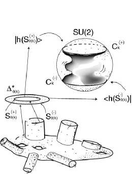
Figure 10: A pictorial rendering of the set up for computing the quantum amplitudes for the cylindrical ends associated with the surface $\partial M$.

The computation of the annulus partition function (58) has been explicitly carried out [12] for the boundary $SU(2)$ CFT at level $\kappa=1$. We restrict our analysis to this particular case and if we apply the results of [12], (see in particular eqn. (4.1) and the accompanying analysis) we get

$$Z_{\Delta_{\theta(i)}^{\ast}}(\{C_{i}^{\pm}\})=\\ =\frac{1}{\sqrt{2}}\sum_{j_{i}\in\frac{1}{2}\mathbb{Z}_{+}}\sum_{m,n}(-1)^{m-n}D_{-m,-n}^{j_{i}}(\widehat{h}^{-1}(S_{\theta(i)}^{(-)}))D_{m,n}^{j_{i}}(\widehat{h}(S_{\theta(i)}^{(+)}))\chi_{j_{i}^{2}}(e^{-\frac{4\pi}{\theta(i)}}),$$ (59)

where

$$\chi_{j_{i}^{2}}(e^{-\frac{4\pi}{\theta(i)}})=\frac{e^{-\frac{4\pi}{\theta(i)}j_{i}^{2}}-e^{-\frac{4\pi}{\theta(i)}(j_{i}+1)^{2}}}{\eta(e^{-\frac{4\pi}{\theta(i)}})}.$$ (60)

is the character of the Virasoro highest weight representation, and

$$\eta(q)\doteq q^{\frac{1}{24}}\prod_{n=1}^{\infty}(1-q^{n}),$$ (61)

is the Dedekind $\eta$-function.

By diagonalizing we can consider $h^{-1}(S_{\theta(i)}^{(-)})h(S_{\theta(i)}^{(+)})$ as an element of the maximal torus in $SU(2)$, i.e., we can write

$$h^{-1}(S_{\theta(i)}^{(-)})h(S_{\theta(i)}^{(+)})=\left(\begin{array}[]{cc}e^{4\pi\sqrt{-1}\lambda(i)}&0\\ 0&e^{-4\pi\sqrt{-1}\lambda(i)}\end{array}\right),$$ (62)

and a representation-theoretic computation [12] eventually provides

$$Z_{\Delta_{\theta(i)}^{\ast}}(\{C_{i}^{\pm}\})=\frac{1}{\sqrt{2}}\sum_{j\in\frac{1}{2}\mathbb{Z}_{+}}\cos(8\pi j_{i}\lambda(i))\frac{e^{-\frac{4\pi}{\theta(i)}j_{i}^{2}}}{\eta(e^{-\frac{4\pi}{\theta(i)}})}.$$ (63)

(Note that ${\alpha}$ in [12] corresponds to our $4\pi\sqrt{-1}\lambda(i)$, hence the presence of $\cos(8\pi j_{i}\lambda(i))$ in place of their $\cosh(2j_{i}\alpha(i))$).

An important point to stress is that, according to the above analysis, the partition function $Z_{\Delta_{\theta(i)}^{\ast}}(\{C_{i}^{\pm}\})$ can be interpreted as the superposition over all possible $j_{i}$ channel amplitudes

$$\partial\Gamma_{i}\longmapsto A(j_{i})\doteq\frac{1}{\sqrt{2}}\cos(8\pi j_{i}\lambda(i))\frac{e^{-\frac{4\pi}{\theta(i)}j_{i}^{2}}}{\eta(e^{-\frac{4\pi}{\theta(i)}})}$$ (64)

that can be associated to the boundary component $\partial\Gamma_{i}$ of the ribbon graph $\Gamma$. Such amplitudes can be interpreted as the various $j_{i}=(n+\lambda(i))$, ($0\leq\lambda(i)\leq\frac{1}{2}$), Virasoro (closed string) modes propagating along the cylinder $\Delta_{\theta(i)}^{\ast}$.

4.2
The Ribbon graph insertion operators

In order to complete the picture, we need to discuss how the $N_{0}$ amplitudes $\{A(j_{i})\}$ defined by (64) interact along $\Gamma$. Such an interaction is described by boundary operators which mediate the change in boundary conditions $|\widehat{h}(S_{\theta(p)}^{(+)})\rangle_{\partial\Gamma_{p}}$ and $|\widehat{h}(S_{\theta(q)}^{(+)})\rangle_{\partial\Gamma_{q}}$ between any two adjacent boundary components $\partial\Gamma_{p}$ and $\partial\Gamma_{q}$, (note that the adjacent boundaries of the ribbon graph are associated with adjacent cells $\rho^{2}(p)$, $\rho^{2}(q)$ of  $|P_{T_{l}}|\rightarrow M$, and thus to the edges $\sigma^{1}(p,q)$ of the triangulation $|T_{l}|\rightarrow M$). In particular, the coefficients of the operator product expansion (OPE), describing the short-distance behavior of the boundary operators on adjacent $\partial\Gamma_{p}$ and $\partial\Gamma_{q}$, will keep tract of the combinatorics associated with $|P_{T_{l}}|\rightarrow{M}$.

To this end, let us consider generic pairwise adjacent 2-cells $\rho^{2}(p)$ , $\rho^{2}(q)$ and $\rho^{2}(r)$ in $|P_{T_{l}}|\rightarrow M$, and the associated cyclically ordered 3-valent vertex $\rho^{0}(p,q,r)\in|P_{T_{l}}|\rightarrow M$. Let $\{U_{\rho^{0}(p,q,r)},w\}$ the coordinate neighborhood of such a vertex, and $\{U_{\rho^{1}(p,q)},z\}$, $\{U_{\rho^{1}(q,r)},z\}$, and $\{U_{\rho^{1}(r,p)},z\}$ the neighborhoods of the corresponding oriented edges, (the $z$’s appearing in distinct $\{U_{\rho^{1}(\circ,\bullet)},z\}$ are distinct). Consider the edge $\rho^{1}(p,q)$ and two (infinitesimally neighboring) points $z_{1}=x_{1}+\sqrt{-1}y_{1}$ and $z_{2}=x_{2}+\sqrt{-1}y_{2}$, $\mathop{\mathrm{R}e}z_{1}=\mathop{\mathrm{R}e}z_{2}$, in the corresponding $U_{\rho^{1}(p,q)}$, with $x_{1}=x_{2}$. Thus, for $y_{1}\rightarrow 0^{+}$ we approach $\partial\Gamma_{p}\cap\rho^{1}(p,q)$ , whereas for $y_{2}\rightarrow 0^{-}$ we approach a point $\ \in\partial\Gamma_{q}\cap\rho^{1}(q,p)$.

Associated with the edge $\rho^{1}(p,q)\$ we have the two adjacent boundary conditions $|\widehat{h}(S_{\theta(p)}^{(+)})\rangle_{\partial\Gamma_{p}}$, and $|\widehat{h}(S_{\theta(q)}^{(+)})\rangle_{\partial\Gamma_{q}}$, respectively describing the given values of the field $\widehat{h}$ on the two boundary components $\partial\Gamma_{p}\cap\rho^{1}(p,q)$ and $\partial\Gamma_{q}\cap\rho^{1}(q,p)$ of $\rho^{1}(p,q)$. At the points $z_{1},z_{2}\in$ $U_{\rho^{1}(p,q)}$ we can consider the insertion of boundary operators $\psi_{j_{(p,q)}}^{j_{q}j_{p}}(z_{1})$ and $\psi_{j_{(q,p)}}^{j_{p}j_{q}}(z_{2})$ mediating between the corresponding boundary conditions, i.e.

$$\psi_{j_{(p,q)}}^{j_{q}j_{p}}(z_{1})|\widehat{h}(S_{\theta(p)}^{(+)})\rangle_{\partial\Gamma_{p}}\underset{y_{1}\rightarrow 0^{+}}{=}|\widehat{h}(S_{\theta(q)}^{(+)})\rangle_{\partial\Gamma_{q}},$$

(65)

$$\psi_{j_{(q,p)}}^{j_{p}j_{q}}(z_{2})|\widehat{h}(S_{\theta(q)}^{(+)})\rangle_{\partial\Gamma_{q}}\underset{y_{2}\rightarrow 0^{-}}{=}|\widehat{h}(S_{\theta(p)}^{(+)})\rangle_{\partial\Gamma_{p}}.$$

Note that $\psi_{j_{(p,q)}}^{j_{q}j_{p}}$ carries the single primary isospin label $j_{(p,q)}$ (also indicating the oriented edge $\rho^{1}(p,q)$ where we are inserting the operator), and the two additional isospin labels $j_{p}$ and $j_{q}$ indicating the two boundary conditions at the two portions of $\partial\Gamma_{p}$ and $\partial\Gamma_{q}$ adjacent to the insertion edge $\rho^{1}(p,q)$.  Likewise, by considering the oriented edges $\rho^{1}(q,r)$ and $\rho^{1}(r,p)$,  we can introduce the operators $\psi_{j_{(r,q)}}^{j_{q}j_{r}}$, $\psi_{j_{(q,r)}}^{j_{r}j_{q}}$, $\psi_{j_{(p,r)}}^{j_{r}j_{p}}$, and $\psi_{j_{(r,p)}}^{j_{p}j_{r}}$. In full generality, we can rewrite the above definition explicitly in terms of the adjacency matrix $B(\Gamma)$ of the ribbon graph $\Gamma$,

$$B_{st}(\Gamma)=\left\{\begin{tabular}[]{lll}$1$&if&$\rho^{1}(s,t)$ is an edge of $\Gamma$\\ &&\\ $0$&&otherwise\end{tabular}\right.,$$ (66)

according to

$$\psi_{j_{(p,q)}}^{j_{q}j_{p}}(z_{1})|\widehat{h}(S_{\theta(p)}^{(+)})\rangle_{\partial\Gamma_{p}}\underset{y_{1}\rightarrow 0^{+}}{=}B_{pq}(\Gamma)|\widehat{h}(S_{\theta(q)}^{(+)})\rangle_{\partial\Gamma_{q}}.$$ (67)

Any such boundary operator, say $\psi_{j_{(p,q)}}^{j_{q}j_{p}}$, is a primary field (under the action of Virasoro algebra) of conformal dimension $H_{j_{(p,q)}}$, and they are all characterized [14], [13], [15] by the following properties dictated by conformal invariance (in the corresponding coordinate neighborhood $U_{\rho^{1}(p,q)}$)

$$\langle 0|\psi_{j_{(p,q)}}^{j_{q}j_{p}}(z_{1})|0\rangle=0,\;\;\langle\widehat{h}(S_{\theta(p)}^{(-)})|\mathbb{I}^{j_{p}j_{p}}|\widehat{h}(S_{\theta(p)}^{(+)})\rangle\;\!=a^{j_{p}j_{p}},$$

$$\langle 0|\psi_{j_{(p,q)}}^{j_{q}j_{p}}(z_{1})\psi_{j_{(q,p)}}^{j_{p}j_{q}}(z_{2})|0\rangle=b_{j_{(p,q)}}^{j_{q}j_{p}}|z_{1}-z_{2}|^{-2H_{j_{(p,q)}}}\delta_{j_{(p,q)}j_{(q,p)}},$$

where $\mathbb{I}^{j_{p}j_{p}}$ is the identity operator, and where $a^{j_{p}j_{p}}$ and $b_{j_{(p,q)}}^{j_{q}j_{p}}$ are normalization factors. In particular, the parameters $b_{j_{(p,q)}}^{j_{q}j_{p}}$ define the normalization of the two-points function. Note that [14] for $SU(2)$ the $b_{j_{(p,q)}}^{j_{q}j_{p}}$ are such that $b_{j_{(p,q)}}^{j_{q}j_{p}}=b_{j_{(q,p)}}^{j_{p}j_{q}}(-1)^{2j_{(p,q)}}$, and are (partially) constrained by the OPE of the $\psi_{j_{(p,q)}}^{j_{q}j_{p}}$. As customary in boundary CFT, we leave such a normalization factors dependence explicit in what follows.

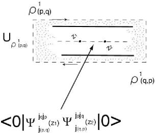
Figure 11: The insertion of boundary operators $\psi_{j_{(p,q)}}^{j_{q}j_{p}}$ in the complex coordinate neighborhood $U_{\rho^{1}(p,q)}$, giving rise to the two-point function in the corresponding oriented edge $\rho^{1}(p,q)$.

In order to discuss the properties of  the $\psi_{j_{(p,q)}}^{j_{q}j_{p}}$ , let us extend the (edges) coordinates $z$  to the unit disk  $U_{\rho^{0}(p,q,r)}$ associated to the generic vertex $\rho^{0}(p,q,r)$, and denote by

$$w_{p} = \frac{\varepsilon}{3}e^{\frac{1}{2}\pi\sqrt{-1}}\in U_{\rho^{0}(p,q,r)}\cap U_{\rho^{1}(p,q)}$$

$$w_{q} = \frac{\varepsilon}{2}e^{\frac{7}{6}\pi\sqrt{-1}}\in U_{\rho^{0}(p,q,r)}\cap U_{\rho^{1}(q,r)}$$ (69)

$$w_{r} = \varepsilon e^{\frac{11}{6}\pi\sqrt{-1}}\in U_{\rho^{0}(p,q,r)}\cap U_{\rho^{1}(r,p)}$$

the coordinates of three points in an $\varepsilon$- neighborhood ($0<\varepsilon<1$) of the vertex $w=0$, (fractions of $\varepsilon$ are introduced for defining a radial ordering; note also that by exploting the coordinate changes (7), one can easily map such points in the upper half planes associated with the edge complex variables $z$ corresponding to $U_{\rho^{1}(p,q)}$, $U_{\rho^{1}(q,r)}$, and $U_{\rho^{1}(r,p)}$, and formulate the theory in a more conventional fashion). To these points we associate the insertion of boundary operators $\psi_{j_{(r,p)}}^{j_{p}j_{r}}(w_{r})$, $\psi_{j_{(q,r)}}^{j_{r}j_{q}}(w_{q})$, $\psi_{j_{(p,q)}}^{j_{q}j_{p}}(w_{p})$ which pairwise mediate among the boundary conditions $|\widehat{h}(S_{\theta(p)}^{(+)})\rangle$, $|\widehat{h}(S_{\theta(q)}^{(+)})\rangle$, and $|\widehat{h}(S_{\theta(r)}^{(+)})\rangle$. The behavior of such insertions at the vertex $\rho^{0}(p,q,r)$, (i.e., as $\varepsilon\rightarrow 0$), is described by the following OPEs (see [13], [14])

$$\psi_{j_{(r,p)}}^{j_{p}j_{r}}(w_{r})\psi_{j_{(q,r)}}^{j_{r}j_{q}}(w_{q})=$$

$$=\sum_{j}C_{j_{(r,p)}j_{(q,r)}j}^{j_{p}j_{r}j_{q}}|w_{r}-w_{q}|^{H_{j}-H_{j_{(r,p)}}-H_{j_{(q,r)}}}(\psi_{j}^{j_{p}j_{q}}(w_{q})+...),$$

$$\psi_{j_{(q,r)}}^{j_{r}j_{q}}(w_{q})\psi_{j_{(p,q)}}^{j_{q}j_{p}}(w_{p})=$$

$$=\sum_{j}C_{j_{(q,r)}j_{(p,q)}j}^{j_{r}j_{q}j_{p}}|w_{q}-w_{p}|^{H_{j}-H_{j_{(q,r)}}-H_{j_{(p,q)}}}(\psi_{j}^{j_{r}j_{p}}(w_{p})+...),$$

$$\psi_{j_{(p,q)}}^{j_{q}j_{p}}(w_{p})\psi_{j_{(r,p)}}^{j_{p}j_{r}}(w_{r})=$$

$$=\sum_{j}C_{j_{(p,q)}j_{(r,p)}j}^{j_{q}j_{p}j_{r}}|w_{p}-w_{r}|^{H_{j}-H_{j_{(p,q)}}-H_{j_{(r,p)}}}(\psi_{j}^{j_{q}j_{p}}(w_{r})+...),$$

where the dots stand for higher order corrections in $|w_{\circ}-w_{\bullet}|$, the $H_{J_{...}}$ are the conformal weights of the corresponding boundary operators, and the $C_{j_{(r,p)}j_{(q,r)}j}^{j_{p}j_{r}j_{q}}$ are the OPE structure constants.

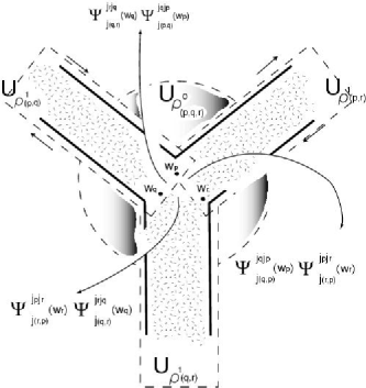
Figure 12: The OPEs between the boundary operators around a given vertex $\rho^{0}(p,q,r)$ in the corresponding complex coordinates neighborhoods $U_{\rho^{0}(p,q,r)}$, $U_{\rho^{1}(p,q)}$, etc..

As is well known [14], the parameters $b_{j_{(p,q)}}^{j_{q}j_{p}}$ and the constants $C_{j_{(r,p)}j_{(q,r)}j}^{j_{p}j_{r}j_{q}}$ are not independent. In our setting this is a consequence of the fact that to the oriented vertex $\rho^{0}(p,q,r)$ we can associate a three-point function which must be invariant under cyclic permutations, i.e.

$$\langle\psi_{j_{(r,p)}}^{j_{p}j_{r}}(w_{r})\psi_{j_{(q,r)}}^{j_{r}j_{q}}(w_{q})\psi_{j_{(p,q)}}^{j_{q}j_{p}}(w_{p})\rangle=\langle\psi_{j_{(p,q)}}^{j_{q}j_{p}}(w_{r})\psi_{j_{(r,p)}}^{j_{p}j_{r}}(w_{q})\psi_{j_{(q,r)}}^{j_{r}j_{q}}(w_{p})\rangle=$$

$$=\langle\psi_{j_{(q,r)}}^{j_{r}j_{q}}(w_{r})\psi_{j_{(p,q)}}^{j_{q}j_{p}}(w_{q})\psi_{j_{(r,p)}}^{j_{p}j_{r}}(w_{p})\rangle.$$

By using the boundary OPE (LABEL:OPE), each term can be computed in two distinct ways, e.g., by denoting with $\underbrace{}$ an OPE pairing, we must have

$$\langle\underbrace{\psi_{j_{(r,p)}}^{j_{p}j_{r}}(w_{r})\psi_{j_{(q,r)}}^{j_{r}j_{q}}(w_{q})}\psi_{j_{(p,q)}}^{j_{q}j_{p}}(w_{p})\rangle=\langle\psi_{j_{(r,p)}}^{j_{p}j_{r}}(w_{r})\underbrace{\psi_{j_{(q,r)}}^{j_{r}j_{q}}(w_{q})\psi_{j_{(p,q)}}^{j_{q}j_{p}}(w_{p})}\rangle$$ (74)

which (by exploiting (LABEL:twopoints)) in the limit $w\rightarrow 0$  provides

$$C_{j_{(r,p)}j_{(q,r)}j_{(p,q)}}^{j_{p}j_{r}j_{q}}b_{j_{(q,p)}}^{j_{p}j_{q}}=C_{j_{(q,r)}j_{(p,q)}j_{(r,p)}}^{j_{r}j_{q}j_{p}}b_{j_{(r,p)}}^{j_{p}j_{r}},$$ (75)

(note that the Kronecker $\delta$ in (LABEL:twopoints) implies that $j_{(q,p)}=j_{(p,q)}$, etc. ). From the OPE evaluation of the remaining two three-points function one similarly obtains

$$C_{j_{(p,q)}j_{(r,p)}j_{(q,r)}}^{j_{q}j_{p}j_{r}}b_{j_{(r,q)}}^{j_{q}j_{r}} = C_{j_{(r,p)}j_{(q,r)}j_{(p,q)}}^{j_{p}j_{r}j_{q}}b_{j_{(p,q)}}^{j_{q}j_{p}},$$

$$C_{j_{(q,r)}j_{(p,q)}j_{(r,p)}}^{j_{r}j_{q}j_{p}}b_{j_{(p,r)}}^{j_{r}j_{p}} = C_{j_{(p,q)}j_{(r,p)}j_{(q,r)}}^{j_{q}j_{p}j_{r}}b_{j_{(q,r)}}^{j_{r}j_{q}}.$$

Since

$$b_{j_{(q,p)}}^{j_{p}j_{q}} = b_{j_{(p,q)}}^{j_{q}j_{p}}(-1)^{2j_{(p,q)}},$$

$$b_{j_{(r,p)}}^{j_{p}j_{r}} = b_{j_{(p,r)}}^{j_{r}j_{p}}(-1)^{2j_{(p,r)}},$$ (77)

$$b_{j_{(q,r)}}^{j_{r}j_{q}} = b_{j_{(r,q)}}^{j_{q}j_{r}}(-1)^{2j_{(r,q)}},$$

one eventually gets

$$C_{j_{(r,p)}j_{(q,r)}j_{(p,q)}}^{j_{p}j_{r}j_{q}}b_{j_{(q,p)}}^{j_{p}j_{q}} = (-1)^{2j_{(q,p)}}C_{j_{(p,q)}j_{(r,p)}j_{(q,r)}}^{j_{q}j_{p}j_{r}}b_{j_{(q,r)}}^{j_{r}j_{q}},$$

$$C_{j_{(p,q)}j_{(r,p)}j_{(q,r)}}^{j_{q}j_{p}j_{r}}b_{j_{(r,q)}}^{j_{q}j_{r}} = (-1)^{2j_{(r,q)}}C_{j_{(q,r)}j_{(p,q)}j_{(r,p)}}^{j_{r}j_{q}j_{p}}b_{j_{(r,p)}}^{j_{p}j_{r}},$$ (78)

$$C_{j_{(q,r)}j_{(p,q)}j_{(r,p)}}^{j_{r}j_{q}j_{p}}b_{j_{(p,r)}}^{j_{r}j_{p}} = (-1)^{2j_{(p,r)}}C_{j_{(r,p)}j_{(q,r)}j_{(p,q)}}^{j_{p}j_{r}j_{q}}b_{j_{(p,q)}}^{j_{q}j_{p}},$$

which are the standard relation between the OPE parameters and the normalization of the 2-points function for boundary $SU(2)$ insertion operators, [14]. Such a lengthy (and slightly pedantic) analysis is necessary to show that our association of boundary insertion operators $\psi_{j_{(r,p)}}^{j_{p}j_{r}}$, to the edges of the ribbon graph $\Gamma$ is actually consistent with $SU(2)$ boundary CFT, in particular that geometrically the correlator $\langle\psi_{j_{(r,p)}}^{j_{p}j_{r}}(w_{r})\psi_{j_{(q,r)}}^{j_{r}j_{q}}(w_{q})\psi_{j_{(p,q)}}^{j_{q}j_{p}}(w_{p})\rangle$   is associated with the three mutually adjacent boundary components $\partial\Gamma_{p}$, $\partial\Gamma_{q}$, and $\partial\Gamma_{r}$ of the ribbon graph $\Gamma$. More generally, let us consider four mutually adjacent boundary components $\partial\Gamma_{p}$, $\partial\Gamma_{q}$, $\partial\Gamma_{r}$, and $\partial\Gamma_{s}$. Their adjacency relations can be organized in two distinct ways labelled by the distinct two vertices they generate: if $\partial\Gamma_{p}$ is adjacent to $\partial\Gamma_{r}$ then  we have the two vertices $\rho^{0}(p,q,r)$ and $\rho^{0}(p,r,s)$ connected by the edge $\rho^{1}(p,r)$; conversely, if $\partial\Gamma_{q}$ is adjacent to $\partial\Gamma_{s}$ then  we have the two vertices $\rho^{0}(p,q,s)$ and $\rho^{0}(q,r,s)$ connected by the edge $\rho^{1}(q,s)$.  It follows that the correlation function of the corresponding four boundary operators, $\langle\psi_{j_{(s,p)}}^{j_{p}j_{s}}\psi_{j_{(r,s)}}^{j_{s}j_{r}}\psi_{j_{(q,r)}}^{j_{r}j_{q}}\psi_{j_{(p,q)}}^{j_{q}j_{p}}\rangle$, can be evaluated by exploiting the ($(S)$-channel) factorization associated with the coordinate neighborhood $\{U_{\rho^{1}(r,p)},z^{(S)}\}$, or, alternatively, by exploiting the ($(T)$-channel) factorization associated with $\{U_{\rho^{1}(q,s)},z^{(T)}\}$.

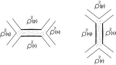
Figure 13: The dual channels in evaluating the correlation function of the four boundary operators corresponding to the four boundary components involved.

From the observation that both such expansions must yield the same result, it is possible [15] to directly relate the OPE coefficients $C_{j_{(r,p)}j_{(q,r)}j_{(p,q)}}^{j_{p}j_{r}j_{q}}$ with the fusion matrices $F_{j_{r}j_{(p,q)}}\left[\begin{array}[]{cc}j_{p}&j_{q}\\ j_{(r,p)}&j_{(q,r)}\end{array}\right]$ which express the crossing duality between four-points conformal blocks. Recall that for WZW models the fusion ring can be identified with the character ring of the quantum deformation $\mathcal{U}_{Q}(\mathbf{g})$ of  the enveloping algebra of $\mathbf{g}$ evaluated at the root of unity given by $Q=e^{\pi\sqrt{-1}/(\kappa+h^{\vee})}$ (where $h^{\vee}$ is the dual Coxeter number and $\kappa$ is the level of the theory). In other words, for WZW models, the fusion  matrices are the $6j$ -symbols of the corresponding (quantum) group. From such remarks, it follows that in our case (i.e., for $\kappa=1$, $h^{\vee}=2$) the structure constants $C_{j_{(r,p)}j_{(q,r)}j_{(p,q)}}^{j_{p}j_{r}j_{q}}$ are suitable entries [16] of the $6j$-symbols of the quantum group $SU(2)_{Q=e^{\frac{\pi}{3}\sqrt{-1}}}$, i.e.

$$C_{j_{(r,p)}j_{(q,r)}j_{(p,q)}}^{j_{p}j_{r}j_{q}}=\left\{\begin{array}[]{ccc}j_{(r,p)}&j_{p}&j_{r}\\ j_{q}&j_{(q,r)}&j_{(p,q)}\end{array}\right\}_{Q=e^{\frac{\pi}{3}\sqrt{-1}}}$$ (79)

4.3 The partition function.

The final step in our construction is to uniformize the local coordinate representation of the ribbon graph $\Gamma$ with the cylindrical metric $\{|\phi(i)|\}$, defined by the quadratic differential $\{\phi(i)\}$. In such a framework, there is a natural prescription for associating to the resulting metric ribbon graph $(\Gamma,\{|\phi(i)|\})$ a factorization of the correlation functions of   the $N_{1}$ insertion operators $\{\psi_{j_{(p,q)}}^{j_{q}j_{p}}\}$, (recall that $N_{1}$ is the number of edges of $\Gamma$). Explicitly, for the generic vertex  $\rho^{0}(p,q,r)$, let  $z_{p}^{(0)}\in U_{\rho^{1}(p,q)}\cap U_{\rho^{0}(p,q,r)}$,  $z_{q}^{(0)}\in U_{\rho^{1}(q,r)}\cap U_{\rho^{0}(p,q,r)}$, and  $z_{r}^{(0)}\in U_{\rho^{1}(r,p)}\cap U_{\rho^{0}(p,q,r)}$ respectively denote the coordinates of the points $w_{p}$, $w_{q}$, and $w_{r}$ (see (69)) in the respective edge uniformizations, and for notational purposes, let us set, (in an $\varepsilon$-neighborhood of $z_{\rho^{0}(p,q,r)}=0\in U_{\rho^{0}(p,q,r)}$),

$$\psi_{j_{(r,p)}}^{j_{p}j_{r}}(\rho^{0}(p,q,r)) \doteq \psi_{j_{(r,p)}}^{j_{p}j_{r}}(z_{r}^{(0)}),$$

$$\psi_{j_{(q,r)}}^{j_{r}j_{q}}(\rho^{0}(p,q,r)) \doteq \psi_{j_{(q,r)}}^{j_{r}j_{q}}(z_{q}^{(0)}),$$ (80)

$$\psi_{j_{(p,q)}}^{j_{q}j_{p}}(\rho^{0}(p,q,r)) \doteq \psi_{j_{(p,q)}}^{j_{q}j_{p}}(z_{p}^{(0)}).$$

Let us consider, (in the limit $\varepsilon\rightarrow 0$ ), the correlation function

$$\left\langle\bigotimes_{i=1}^{N_{0}(T)}\partial\Gamma_{i};\otimes j_{i}\right\rangle\doteq$$

$$\doteq\left\langle\prod_{\{\rho^{0}(p,q,r)\}}^{N_{2}(T)}\psi_{j_{(r,p)}}^{j_{p}j_{r}}(\rho^{0}(p,q,r))\psi_{j_{(q,r)}}^{j_{r}j_{q}}(\rho^{0}(p,q,r))\psi_{j_{(p,q)}}^{j_{q}j_{p}}(\rho^{0}(p,q,r))\right\rangle,$$

where  the product runs over the $N_{2}(T)$ vertices $\{\rho^{0}(p,q,r)\}$  of $\Gamma$. We can factorize it along the $N_{1}(T)$ channels generated by the edge cordinate neighborhoods $\{U_{\rho^{1}(p,q)}\}$ according to

$$\left\langle\bigotimes_{i=1}^{N_{0}(T)}\partial\Gamma_{i};\otimes j_{i}\right\rangle=$$

$$=\sum_{\{j_{(r,p)}\}}\prod_{\{\rho^{0}(p,q,r)\}}^{N_{2}(T)}\underset{\rho^{0}(p,q,r)}{\left\langle\psi_{j_{(r,p)}}^{j_{p}j_{r}}\psi_{j_{(q,r)}}^{j_{r}j_{q}}\psi_{j_{(p,q)}}^{j_{q}j_{p}}\right\rangle}\prod_{\{\rho^{1}(p,r)\}}^{N_{1}(T)}\underset{\rho^{1}(p,r)}{\left\langle\psi_{j_{(r,p)}}^{j_{p}j_{r}}\psi_{j_{(p,r)}}^{j_{r}j_{p}}\right\rangle}$$

where we have set

$$\underset{\rho^{0}(p,q,r)}{\left\langle\psi_{j_{(r,p)}}^{j_{p}j_{r}}\psi_{j_{(q,r)}}^{j_{r}j_{q}}\psi_{j_{(p,q)}}^{j_{q}j_{p}}\right\rangle}\doteq$$

$$\doteq\left\langle\psi_{j_{(r,p)}}^{j_{p}j_{r}}(\rho^{0}(p,q,r))\psi_{j_{(q,r)}}^{j_{r}j_{q}}(\rho^{0}(p,q,r))\psi_{j_{(p,q)}}^{j_{q}j_{p}}(\rho^{0}(p,q,r))\right\rangle,$$

$$\underset{\rho^{1}(p,r)}{\left\langle\psi_{j_{(r,p)}}^{j_{p}j_{r}}\psi_{j_{(p,r)}}^{j_{r}j_{p}}\right\rangle}\doteq\left\langle\psi_{j_{(r,p)}}^{j_{p}j_{r}}(\rho^{0}(p,q,r))\psi_{j_{(p,r)}}^{j_{r}j_{p}}(\rho^{0}(p,r,s))\right\rangle,$$ (84)

and where the summation runs over all $N_{1}(T)$ primary highest weight representation $\widehat{\mathfrak{su}}(2)_{\kappa=1}$, labelling the intermediate edge channels $\{j_{(r,p)}\}$. Note that according to (LABEL:twopoints) we can write

$$\underset{\rho^{1}(p,r)}{\left\langle\psi_{j_{(r,p)}}^{j_{p}j_{r}}\psi_{j_{(p,r)}}^{j_{r}j_{p}}\right\rangle}=b_{j_{(r,p)}}^{j_{p}j_{r}}L(p,r)^{-2H_{j_{(r,p)}}},$$ (85)

(recall that $j_{(r,p)}=j_{(p,r)}$), where $L(p,r)$ denotes the length of the edge $\rho^{1}(p,r)$ in the uniformization $(U_{\rho^{1}(p,r)},\{|\phi(i)|\})$. Moreover,  since (see (75))

$$\underset{\rho^{0}(p,q,r)}{\left\langle\psi_{j_{(r,p)}}^{j_{p}j_{r}}\psi_{j_{(q,r)}}^{j_{r}j_{q}}\psi_{j_{(p,q)}}^{j_{q}j_{p}}\right\rangle}=C_{j_{(r,p)}j_{(q,r)}j_{(p,q)}}^{j_{p}j_{r}j_{q}}b_{j_{(q,p)}}^{j_{p}j_{q}},$$ (86)

we get for the boundary operator correlator associated with the ribbon graph $\Gamma$ the expression

$$\left\langle\bigotimes_{i=1}^{N_{0}(T)}\partial\Gamma_{i};\otimes j_{i}\right\rangle=$$

$$=\sum_{\{j_{(r,p)}\}}\prod_{\{\rho^{0}(p,q,r)\}}^{N_{2}(T)}C_{j_{(r,p)}j_{(q,r)}j_{(p,q)}}^{j_{p}j_{r}j_{q}}b_{j_{(q,p)}}^{j_{p}j_{q}}\prod_{\{\rho^{1}(p,r)\}}^{N_{1}(T)}b_{j_{(r,p)}}^{j_{p}j_{r}}L(p,r)^{-2H_{j_{(r,p)}}}.$$

By identifying each $C_{j_{(r,p)}j_{(q,r)}j_{(p,q)}}^{j_{p}j_{r}j_{q}}$ with the corresponding $6j$-symbol, and observing that each normalization factor $b_{j_{(q,p)}}^{j_{p}j_{q}}$ occurs exactly twice, we eventually obtain

$$\left\langle\bigotimes_{i=1}^{N_{0}(T)}\partial\Gamma_{i};\otimes j_{i}\right\rangle=$$

$$\sum_{\{j_{(r,p)}\}}\prod_{\{\rho^{0}(p,q,r)\}}^{N_{2}(T)}\left\{\begin{array}[]{ccc}j_{(r,p)}&j_{p}&j_{r}\\ j_{q}&j_{(q,r)}&j_{(p,q)}\end{array}\right\}_{Q=e^{\frac{\pi}{3}\sqrt{-1}}}\prod_{\{\rho^{1}(p,r)\}}^{N_{1}(T)}\left(b_{j_{(r,p)}}^{j_{p}j_{r}}\right)^{2}L(p,r)^{-2H_{j_{(r,p)}}}.$$ (91)

As the notation suggests,  such a correlator has a residual dependence on the representation labels $\{j_{i}\}$. In other words, it can be considered as an element of the tensor product $\mathcal{H}(\partial\Gamma)=$ $\otimes_{i=1}^{N_{0}(T)}\mathcal{H}_{(i)}$. It is then natural to interpret its evaluation over the amplitudes $\{A(j_{i})\}$ defined by ( 64) as the partition function $Z^{WZW}(|P_{T_{l}}|,\{\widehat{h}(S_{\theta(i)}^{(+)})\})$ associated with the quantum amplitude (55), and describing the $SU(2)$ WZW model (at level $\kappa=1$) on a random Regge polytope $|P_{T_{l}}|\rightarrow M$. By inserting the $N_{0}(T)$ amplitudes $\{A(j_{i})\}$ into (LABEL:graphA), and summing over all possible representation indices $\{j_{p}\}$ we immediately get

$$Z^{WZW}(|P_{T_{l}}|,\{\widehat{h}(S_{\theta(i)}^{(+)})\})=$$

$$=\left(\frac{1}{\sqrt{2}}\right)^{N_{0}(T)}\sum_{\{j_{p}\in\frac{1}{2}\mathbb{Z}_{+}\}}\sum_{\{j_{(r,p)}\}}\prod_{\{\rho^{0}(p,q,r)\}}^{N_{2}(T)}\left\{\begin{array}[]{ccc}j_{(r,p)}&j_{p}&j_{r}\\ j_{q}&j_{(q,r)}&j_{(p,q)}\end{array}\right\}_{Q=e^{\frac{\pi}{3}\sqrt{-1}}}\cdot$$ (94)

$$\cdot\prod_{\{\rho^{1}(p,r)\}}^{N_{1}(T)}\left(b_{j_{(r,p)}}^{j_{p}j_{r}}\right)^{2}L(p,r)^{-2H_{j_{(r,p)}}}\cos(8\pi j_{p}\lambda(i))\frac{e^{-\frac{4\pi}{\theta(i)}j_{p}^{2}}}{\eta(e^{-\frac{4\pi}{\theta(i)}})},$$

where the summation $\sum_{\{j_{p}\in\frac{1}{2}\mathbb{Z}_{+}\}}$ is over all possible $N_{0}(T)$ channels $j_{p}$ describing the Virasoro (closed string) modes propagating along the cylinders $\{\Delta_{\theta(p)}^{\ast}\}_{p=1}^{N_{0}(T)}$. This is the partition function of our WZW model on a random Regge triangulation. The WZW fields are still present through their boundary labels $\lambda(i)$, (which can take the values $0,1/2$), wheras the metric geometry of the polytope enters explicitly both with the edge-length terms $L(p,r)^{-2H_{j_{(r,p)}}}$ and with the conical angle factors $\frac{e^{-\frac{4\pi}{\theta(i)}j_{p}^{2}}}{\eta(e^{-\frac{4\pi}{\theta(i)}})}$. The expression of $Z^{WZW}(|P_{T_{l}}|,\{\widehat{h}(S_{\theta(i)}^{(+)})\})$, also shows the mechanism through which the $SU(2)$ fields couple with simplicial curvature: the coupling amplitudes $\{A(j_{i})\}$ can be interpreted as describing a closed string emitted by $\partial\Gamma_{i}\simeq S_{\theta(i)}^{(-)}$, or rather by the $\overline{S_{\theta(i)}^{2}}$  brane image of this boundary component in $SU(2)$, and absorbed by the brane $S_{\theta(i)}^{2}$ image of the outer boundary $S_{\theta(i)}^{(+)}$, (the curvature carrying vertex). This exchange of closed strings between $2$-branes in  $SU(2)\simeq S^{3}$ describes the interaction of the quantum $SU(2)$ field with the classical gravitational background associated with the edge-length assignments $\{L(p,r)\}$, and with the deficit angles $\{\varepsilon(i)\doteq 2\pi-\theta(i)\}$.

5
Concluding remarks

We note on passing that, in the above framework, 2D gravity can be promoted to a dynamical role by summing (94) over all possible Regge polytopes (i.e., over all possible metric ribbon graphs $\{\Gamma,\{L(p,r)\}\}$). It is clear, from the edge-lenght dependence in (94), that the formal Regge functional measure $\propto\prod_{\{\rho^{1}(p,r)\}}dL(p,r)$, involved in such a summation, inherits an anomalous scaling related to the presence of the weighting factor (to be summed over all isospin channels $j(r,p)$)

$$\prod_{\{\rho^{1}(p,r)\}}^{N_{1}(T)}L(p,r)^{-2H_{j_{(r,p)}}},$$ (95)

where the exponents $\{H_{j_{(r,p)}}\}$ characterize the conformal dimension of the boundary insertion operators $\{\psi_{j_{(r,p)}}^{j_{p}j_{r}}\}$. A dynamical triangulation prescription (i.e., holding fixed the $\{l(p,r)\}$ and simply summing over all possible topological ribbon graphs $\{\Gamma\}$) feels such a scaling more directly via the two-point function (LABEL:twopoints), and (85)(again to be summed over all possible isospin channels $j(r,p)$) which exhibit the same exponent dependence. Even if of great conceptual interest (for a non-critical string view-point), we do not pursue such an analysis here. We are more interested in discussing, at least at a preliminary level, how (94) relates with the bulk dynamics in the double $\widetilde{V}_{M}$ of the 3-manifold $V_{M}$ associated with the triangulated surface $M$. Since we are in a discretized setting, such a connection manifests itself, not surprisingly, with an underyling structure of $\ Z^{WZW}(|P_{T_{l}}|,\{\widehat{h}(S_{\theta(i)}^{(+)})\})$ which directly calls into play, via the presence of the (quantum) $6j$-symbols, the building blocks of the Turaev-Viro construction. This latter theory is an example of topological, or more properly, of a cohomological model. When there are no boundaries, it is characterized by a small (finite dimensional) Hilbert space of states; in the presence of boundaries, however, cohomology increases and the model provides an instance of a holographic correspondence where the space of conformal blocks of the boundary theory (i.e., the space of pre-correlators of the associated CFT) can be also understood as the space of physical states of the bulk topological field theory. A boundary on a Riemann surface, for instance, makes the cohomology bigger and this is precisely the case we are dealing with since we are representing a (random Regge) triangulated surface $|T_{l}|\rightarrow M$  by means of a Riemann surface with cylindrical ends. Thus, we come to a full circle: the boundary discretized degrees of freedom of the $SU(2)$ WZW theory coupled with the discretized metric geometry of the supporting surface, give rise to all the elements which characterize the discretized version of the Chern-Simons bulk theory on $\widetilde{V}_{M}$. What is the origin of such a Chern-Simons model? The answer lies in the observation that by considering $SU(2)$ valued maps on a random Regge polytope, the natural outcome is not just a WZW model generated according to the above prescription. The decoration of the pointed Riemann surface $((M;N_{0}),\mathcal{C})$ with the quadratic differential $\phi$, naturally couples the model with a gauge field $A$. In order to see explicitly how this coupling works, we observe that on the Riemann surface with cylindrical ends $\partial M$, associated with the Regge polytope $|P_{T_{l}}|\rightarrow{M}$, we can introduce $\mathfrak{su}(2)$ valued flat gauge potentials $A_{(i)}$ locally defined by

$$A_{(i)}\doteq\gamma_{i}\left[\sqrt{\phi(i)}\left(\frac{\lambda(i)}{\kappa}\mathbf{\sigma}_{3}\right)-\frac{\sqrt{-1}}{2\pi}L(i)\left(\frac{\lambda(i)}{\kappa}\mathbf{\sigma}_{3}\right)d\ln\left|\zeta(i)\right|\right]\gamma_{i}^{-1}=$$

$$=\frac{\sqrt{-1}}{4\pi}L(i)\gamma_{i}\left(\frac{\lambda(i)}{\kappa}\mathbf{\ \sigma}_{3}\right)\gamma_{i}^{-1}\left(\frac{d\zeta(i)}{\zeta(i)}-\frac{d\overline{\zeta}(i)}{\overline{\zeta}(i)}\right),$$

around each cylindrical end $\Delta_{\theta(i)}^{\ast}$ of base circumference $L(i)$, and where $\gamma_{i}\in SU(2)$. (It is worthwhile to note that the geometrical role of    the connection $\{A_{(i)}\}$ is more properly seen as the introduction, on the cohomology group $H^{1}((M,N_{0});\mathcal{C})$ of the pointed Riemann surface $((M,N_{0});\mathcal{C})$, of an Hodge structure analogous to the classical Hodge decomposition of $H^{h}(M;\mathcal{C})$ generated by the spaces $\mathcal{H}^{r,h-r}$ of harmonic $h$-forms on $(M;\mathcal{C})$ of type $(r,h-r)$. Such a decomposition does not hold, as it stands, for punctured surfaces since $H^{1}((M,N_{0});\mathcal{C})$ can be odd-dimensional, but it can be replaced by the mixed Deligne-Hodge decomposition). The action $S_{|T_{l=a}|}^{WZW}(\eta)$ gets correspondingly dressed according to a standard prescription (see e.g. [11]) and one is rather naturally led to the familiar correspondence between states of the bulk Chern-Simons theory associated with the gauge field $A$, and the correlators of the boundary WZW model.

Let us also stress that the relation between (94) and a triangulation of the bulk 3-manifold $\widetilde{V}_{M}$, say, the association of tetrahedra to the (quantum) $6j$-symbols characterized by (79), is rather natural under the doubling procedure giving rise to $\widetilde{V}_{M}$ and to the Schottky double $M^{D}$. Under such doubling, the trivalent vertices $\{\rho^{0}(p,q,r)\}$ of  $|P_{T_{l}}|\rightarrow{M}$ yield two preimages in $\widetilde{V}_{M}$, say $\sigma_{(3)}^{0}(\alpha)$ and $\sigma_{(3)}^{0}(\beta)$, whereas the outer boundaries $S_{\theta(p)}^{(+)}$, $S_{\theta(q)}^{(+)}$, $S_{\theta(r)}^{(+)}$ associated with the vertices $\sigma^{0}(p)$, $\sigma^{0}(q)$, and $\sigma^{0}(r)$ in $|T_{l}|\rightarrow M$ are left fixed under the involution $\Upsilon$ defining $M^{D}$. Fix our attention on $\sigma_{(3)}^{0}(\alpha)$, and let us consider the tetrahedron $\sigma_{(3)}^{3}(p,q,r,\alpha)$ with base the triangle $\sigma^{2}(p,q,r)\in|T_{l}|\rightarrow M$ and apex $\sigma_{(3)}^{0}(\alpha)$. According to our analysis of the insertion operators $\{\psi_{j_{(r,p)}}^{j_{p}j_{r}}\}$, to the edges $\sigma^{1}(p,q)$, $\sigma^{1}(q,r)$, and $\sigma^{1}(r,p)$ of the triangle $\sigma^{2}(p,q,r)$ we must associate the primary labels $j(p,q)$, $j(q,r)$, and $j(r,p)$, respectively. Similarly, it is also natural to associate with the edges $\sigma_{(3)}^{1}(p,\alpha)$, $\sigma_{(3)}^{1}(q,\alpha)$, and $\sigma_{(3)}^{1}(r,\alpha)$ the labels $j_{p}$, $j_{q}$, and $j_{r}$, respectively. Thus, we have the tetrahedron labelling

$$\sigma_{(3)}^{3}(p,q,r,\alpha)\longmapsto\left(j(p,q),j(q,r),j(r,p);j_{p},j_{q},j_{r}\right).$$ (97)

The standard prescription for associating the (quantum) $6j$-symbols to a $SU(2)_{Q}$-labelled tetrahedron such as $\sigma_{(3)}^{3}(p,q,r,\alpha)$ provides

$$\sigma_{(3)}^{3}(p,q,r,\alpha)\longmapsto\left\{\begin{array}[]{ccc}j_{(q,p)}&j_{p}&j_{q}\\ j_{r}&j_{(q,r)}&j_{(p,r)}\end{array}\right\}_{Q=e^{\frac{\pi}{3}\sqrt{-1}}},$$ (98)

which (up to symmetries) can be identified with (79).  In this connection, one can observe that the partition function (94) has a formal structure not too dissimilar (in its general representation theoretic features) from the boundary partition function discussed in [5], but we postpone to a forthcoming paper a detailed analysis of such a correspondence since it needs to be framed within the broader context of a study of the properties of the Chern-Simons bulk states associated to (94).

Acknowledgements

This work was supported in part by the Ministero dell’Universita’ e della Ricerca Scientifica under the PRIN project The geometry of integrable systems. The work of G. Arcioni is supported in part by the European Community’s Human Potential Programme under contract HPRN-CT-2000-00131 Quantum Spacetime. M. Carfora is grateful to P. Di Francesco and N. Kawamoto for constructive remarks at early stages of this work.

References

[1]
G. ’t Hooft,
“The scattering matrix approach for the quantum black hole: An overview,”
Int. J. Mod. Phys. A 11 (1996) 4623
[arXiv:gr-qc/9607022].
[2]
G. ’t Hooft,
“TransPlanckian particles and the quantization of time,”
Class. Quant. Grav. 16 (1999) 395
[arXiv:gr-qc/9805079].
[3]
G. ’t Hooft,
“Quantum gravity as a dissipative deterministic system,”
Class. Quant. Grav. 16 (1999) 3263
[arXiv:gr-qc/9903084].
[4]
T. Regge and R. M. Williams,
“Discrete Structures In Gravity,”
J. Math. Phys. 41 (2000) 3964
[arXiv:gr-qc/0012035].
[5] G. Arcioni, M. Carfora, A. Marzuoli and M. O’Loughlin,
“Implementing holographic projections in Ponzano-Regge gravity,”
Nucl. Phys. B 619 (2001) 690
[arXiv:hep-th/0107112].
[6]
L. Freidel and K. Krasnov,
“2D conformal field theories and holography,”
[arXiv:hep-th/0205091],
M. O’Loughlin,
“Boundary actions in Ponzano-Regge discretization, quantum groups and AdS(3),”
[arXiv:gr-qc/0002092],
D. Oriti,
“Boundary terms in the Barrett-Crane spin foam model and consistent gluing,”
Phys. Lett. B 532 (2002) 363
[arXiv:gr-qc/0201077].
[7] N. Kawamoto, H. B. Nielsen, N. Sato, “Lattice Chern-Simons gravity via Ponzano-Regge model”,
Nuc. Phys. B 555 (1999) 629.
[8] M. Carfora, A. Marzuoli, “Conformal modes in simplicial quantum
gravity and the Weil-Petersson volume of moduli space”, [arXiv:math-ph/0107028]
Adv.Math.Theor.Phys. 6(2002) 357.
[9] M. Carfora, C. Dappiaggi, A. Marzuoli, “The modular geometry of
random Regge triangulations”, [arXiv:gr-qc/0206077] Class. Quant. Grav. 19(2002) 5195.
[10] M. Carfora, “Discretized Gravity and the SU(2) WZW model”, to appear in Class. Quant. Grav. (2003).
[11] K. Gawȩdzki, “Conformal field theory: a case study”. In: ”Conformal Field Theory”,
Frontiers in Physics 102, eds. Nutku, Y.,
Saclioglu, C., Turgut, T., Perseus Publ., Cambridge Ma. (2000), 1-55.
[12] M.R. Gaberdiel, A. Recknagel, G.M.T. Watts,
“The conformal boundary states for SU(2) at level 1”, Nuc. Phys. B 626 (2002) 344 [hep-th/0108102].
[13] D.C. Lewellen, “Sewing constraints for conformal field
theories on surfaces with boundaries”,
Nuc. Phys. B 372 (1992) 654.
[14] G. Pradisi, A. Sagnotti, Ya. S. Stanev,
“Completeness conditions for boundary operators in 2D conformal field
theory”,
Phys. Lett. B 381 (1996) 97.
[15]
G. Felder, J. Frohlich, J. Fuchs and C. Schweigert,
“The geometry of WZW branes,”
J. Geom. Phys. 34 (2000) 162
[arXiv:hep-th/9909030].
[16] L. Alvarez-Gaumé, C. Gomez, G. Sierra,
“Quantum group interpretation of some conformal field theories”, Phys. Lett. B 220 (1989) 142.
[17] J. Ambjörn, B. Durhuus, T. Jonsson, “Quantum Geometry”,
Cambridge Monograph on Mathematical Physics, Cambridge Univ. Press
(1997).
[18] M. Mulase, M. Penkava, “Ribbon graphs, quadratic differentials on
Riemann surfaces, and algebraic curves defined over”,
The Asian Journal of Mathematics 2, 875-920 (1998) [math-ph/9811024 v2].
[19] W. P. Thurston, “Three-Dimensional Geometry and Topology” ,(ed. By S. Levy), Princeton Math. Series, Princeton Univ. Press, Princeton, New Jersey (1997).
[20]
E. Witten,
“Nonabelian Bosonization In Two Dimensions,”
Commun. Math. Phys. 92 (1984) 455.
[21]
A. Yu. Alekseev, V. Schomerus,
“D-branes in the WZW model”,
Phys.Rev. D60 061901 hep-th/9812193.
[22]
K. Gawedzki,
“Boundary WZW, G/H, G/G and CS theories,”
Annales Henri Poincare 3 (2002) 847
[arXiv:hep-th/0108044].
[23] V. Schomerus,
“Lectures on branes in curved backgrounds,”
Class. Quant. Grav. 19 (2002) 5781
[arXiv:hep-th/0209241].
[24]
M. R. Gaberdiel,
“D-Branes From Conformal Field Theory,”
Fortsch. Phys. 50 (2002) 783.