Neutrino damping rate at finite temperature and density

Abstract

A first principle derivation is given of the neutrino damping rate in real-time thermal field theory. Starting from the discontinuity of the neutrino self energy at the two loop level, the damping rate can be expressed as integrals over space phase of amplitudes squared, weighted with statistical factors that account for the possibility of particle absorption or emission from the medium. Specific results for a background composed of neutrinos, leptons, protons and neutrons are given. Additionally, for the real part of the dispersion relation we discuss the relation between the results obtained from the thermal field theory, and those obtained by the thermal average of the forward scattering amplitude.

I Introduction

A neutrino propagating in matter do not longer respect the vacuum energy momentum relation. The modification of the neutrino dispersion relation is caused by their coherent interaction with the particles in the background and can be accounted in terms of an index of refraction [1] or an effective potential [2]. The topic of neutrino propagation in matter became of prime relevance after Wolfenstein [3] study of the neutrino refractive index in matter, and later when Mikheyev-Smirnov [4] recognized the resonant neutrino flavor oscillations triggered by matter effects. The Mikheyev-Smirnov effect has become the most popular explanation of the solar neutrino deficit [5].

In general, the neutrino dispersion relation is a complex function $\omega_{\kappa}=\omega(\vec{\kappa})$. According to the Thermal Field Theory (TFT) matter contributions to the real and imaginary parts of $\omega(\vec{\kappa})$ arise from the temperature and density-dependent part of the neutrino self-energy. To leading order in $(g^{2}/M_{W}^{2})$ the real part of the dispersion relation is proportional to the particle-antiparticle asymmetry in the background. If the asymmetry is small or zero the imaginary part of $\omega(\kappa)$ and corrections of order $g^{2}/M_{W}^{4}$ to the real part may be important because they do not depend on the differences between the number of particles and antiparticles. This may be the case in the early Universe, when the medium was probably nearly CP-symmetric.

Special attention has been given to the calculations of the $O(g^{2}/M_{W}^{4})$ corrections to the real part of the neutrino dispersion relations [6, 7, 8]. Within the framework of the TFT these corrections arise from the momentum-dependent terms of the boson propagator in the self-energy diagrams.

The imaginary part of the index of refraction for neutrinos propagating in a CP-symmetric plasma composed of electrons, neutrinos and their anti-particles has been considered in references [6, 9, 10]. These calculations have been based upon the computation of the neutrino reaction rates, assuming massless background fermions. In our opinion the relation of the neutrino damping rate to the self-energy discontinuties deserves further consideration. Additionally this work addresses the effects of the nucleons background contributions and the fermion mass correction.

A systematic method to compute the damping rate from the imaginary part of the self energy can be formulated in terms of the Cuttosky thermal rules. Weldon [11] and Kobes [12] proved that the imaginary part of the self energy can be organized in a form that includes square of amplitudes of the various processes obtained from the cuts of the self energy and weighted with the appropriated statistical factors. The examples discussed in those papers are always at the one loop level. As it shall be discussed, the calculation of the neutrino damping rate require to consider the self energy at the two loop level, the interpretation in terms of square of amplitudes of the allowed processes will be proved to remain valid. The approximations required to recover the results obtained from the optical theorem will be clearly stated.

In this work we use the method of real-time thermal field theory to carry out a carefully calculation of the imaginary part of the neutrino dispersion relation in a medium composed of electrons, protons, neutrons, neutrinos and their anti-particles. As already mentioned the contributions to the imaginary part of the neutrino self-energy vanishes at the one loop level, so we have to consider the contributions at the two loops level.

The paper is organized as follows. In the next section we briefly review those ingredients of the FTF formalism that are required to accomplish our calculations. In Section III we re-derive the real part of the dispersion relation of a massless neutrino that propagate in a thermal background. We prove that utilizing the methods of finite -temperature field theory (at the $g^{2}$ order), the neutrino effective potential reduces to the thermal average of neutrino forward scattering amplitude. The calculation of the imaginary part of the dispersion relation is presented in Section IV. The neutrino damping rate is extracted from the discontinuity of self-energy at the two loop level, it is expressed in terms of integrals over space phase of amplitudes squared, weighted with statistical factors that account for the possibility of particle absorption or emission from the medium. Specific results for a background composed of neutrinos, leptons, protons and neutrons are given. The last section contains a summary of our main results.

II Basic formalism

The relevant quantity is the self-energy $\Sigma$, which embodies the effects of the background on a neutrino that propagates through it. According to the real-time formalism of the TFT [13, 14, 15], the real and imaginary part of $\Sigma$ are given by the formulas

$${\rm Re}\,\Sigma={\rm Re}\,{\Sigma}_{11}\,,$$ (1)

$${\rm Im}\,\Sigma={{\Sigma}_{12}\over{2i\left(\eta_{f}(k\cdot u)-\theta(-k\cdot u)\right)}}\,,$$ (2)

where $\Sigma_{ab}$ (a,b = 1,2) are the complex elements of the $2\times 2$ self-energy matrix to be computed utilizing the Feynman rules of the theory. $\theta$ is the step function and

$$\eta_{f}(k\cdot u)=\left[\theta(k\cdot u)n_{f}(x_{k})\,+\,\theta(-k\cdot u)n_{f}(-x_{k})\right]\,,$$ (3)

where the thermal distribution is given by

$$n_{f}(x_{k})={1\over{e^{x_{k}}+1}}\,,$$ (4)

with $x_{k}=\beta(k\cdot u-\mu_{f})$. Here, $\beta$ is the inverse of the temperature and $\mu_{f}$ is the chemical potential associated with the fermion $f$. We have introduced the velocity four-vector of the background $u^{\mu}$. In its own rest frame $u^{\mu}=(1,{\bf 0})$ and the components of the neutrino momentum $k^{\mu}$ are $k^{\mu}=(\omega,\vec{\kappa})$.

In the presence of a medium the chiral nature of the neutrino interactions implies that the self-energy of a massless (left-handed) neutrino is of the form [16]

$$\Sigma(k)=(a{k\mkern-9.0mu/}+b{u\mkern-9.0mu/})L\,,$$ (5)

where $L=(1-\gamma_{5})/2$ and $a$, $b$ are complex functions of the scalars

$$\omega=k\cdot u,\ \ \ \ \ \ \kappa=\sqrt{\omega^{2}-k^{2}}\,.$$ (6)

In this case, the Dirac equation for the spinor $U$ of the neutrino mode in the medium is

$$\left({k\mkern-9.0mu/}-\Sigma\right)U=0\,,$$ (7)

which has non-trivial solutions only for those values of $\omega$ and $\kappa$ such that $V^{2}=0$, with $V_{\mu}=(1-a)k_{\mu}-bu_{\mu}$. Then, the dispersion relations $\omega_{\kappa}$ of the neutrino and antineutrino modes are obtained as the solutions of

$$f(\omega_{\kappa},\kappa)=0,$$ (8)

and

$$\overline{f}(\omega_{\kappa},\kappa)=0\,,$$ (9)

where

$$f(\omega,\kappa) = (1-a)(\omega-\kappa)-b\,,$$ (10)

$$\overline{f}(\omega,\kappa) = (1-a)(\omega+\kappa)-b\,.$$ (11)

In general, the solutions $\omega_{\kappa}$ are complex, as usual we write

$$\omega_{\kappa}=\omega_{r}-i\gamma/2,$$ (12)

where both $\omega_{r}={\rm Re}\,\omega_{\kappa}$ and $\gamma=-2\,{\rm Im}\,\omega_{\kappa}$ are real functions of $\kappa$. A consistent interpretation in terms of the dispersion relation for a mode propagating through a medium is possible only if the imaginary part of $\omega_{\kappa}$ is small compared to its real part. In this case the mode can be visualized as a particle (or antiparticle) with an energy $\omega_{r}$ and a damping $\gamma$. Under such assumptions, each one of Eqs. (8) and (9) yields two distinct solutions, one with positive energy and the other with negative energy, whose physical interpretation has been discussed in detail in Ref [16]. Here we will concentrate on the solution of Eq. (8) having a positive real part, which corresponds to the neutrino mode with energy $\omega_{r}$, but similar considerations and results apply to the other solutions.

It is convenient to make the decompositions $a=a_{r}+ia_{i}$ and $b=b_{r}+ib_{i}$. Then, using Eqs. (10) and (12), expanding in powers of $\gamma$ and retaining only terms that are at most linear in $\gamma,a_{i}$ and $b_{i}$, from Eq. (8) we obtain

$$f_{r}(\omega_{r},\kappa)=0\,,$$ (13)

and

$$\frac{\gamma}{2}=\left[\frac{f_{i}(\omega,\kappa)}{\frac{\partial f_{r}}{\partial\omega}}\right]_{\omega=\omega_{r}}\,,$$ (14)

with

$$f_{r} = (1-a_{r})(\omega-\kappa)-b_{r}\,,$$ (15)

$$f_{i} = -a_{i}(\omega-\kappa)-b_{i}.$$ (16)

Only approximate analytical solutions of Eq. (13) are known [16]. At the one-loop level both $b_{r}(\omega_{r},\kappa)$ and $a_{r}(\omega_{r},\kappa)$ are of order $g^{2}/M_{W}^{2}$. Therefore, to this order the energy of a massless neutrino is

$$\omega_{r}\cong\kappa+b_{r}(\omega_{r},\kappa){\big{|}}_{\omega_{r}=\kappa}\,.$$ (17)

On the other hand, as we will show, the imaginary part of $\Sigma$ vanish to $O(g^{2})$ and to this order there are not contributions to ${\rm Im}\,\omega_{\kappa}$. For the perturbative solution of Eq. (14) around $\omega_{r}=\kappa$, we have

$${\gamma\over 2}\cong-b_{i}(\omega_{r},\kappa){\big{|}}_{\omega_{r}=\kappa}\,,$$ (18)

with $b_{i}(\omega_{r},\kappa)$ of $O(g^{4}/M_{W}^{4})$.

The matter effects on the neutrino oscillations are conveniently incorporated by means of the effective potential $V$. This can be introduced by subtracting the (vacuum) kinetic energy from the real part of the neutrino dispersion relation[8]:

$$V\equiv\omega_{r}-\kappa\cong b_{r}(\omega_{r},\kappa){\big{|}}_{\omega_{r}=\kappa}\,.$$ (19)

In the literature it is also customary to use a refraction index, which is defined by

$$n(\kappa)\equiv{\kappa\over\omega_{\kappa}}.$$ (20)

In the approximation we are working on, and utilizing Eqs. (12-19), it follows that its real and imaginary parts are related to the effective potential and the damping rate by

$${\rm Re}\,n(\kappa) \cong 1-{V\over\kappa}\,,$$ (21)

$${\rm Im}\,n(\kappa) \cong {\gamma\over 2\kappa}\,,$$ (22)

with $V$ and $\gamma$ given by Equations (19) and (18), respectively.

III Effective Potential

According to Eq. (19), for a perturbative solutions of the dispersion relation around the vacuum value $\omega_{r}=\kappa$, the effective potential is given by the real part of the coefficient of ${u\mkern-9.0mu/}$ in the neutrino self-energy. This is only true in the lowest order, in general, $V$ will also receive contributions from $a_{r}$. From Eq. (5), it is easy to see that

$$b_{r}(\omega,\kappa)={1\over 4}{\rm Tr}\left\{{{\lambda\mkern-9.0mu/}{\rm Re}\Sigma}\right\}\,.$$ (23)

with

$${\lambda\mkern-9.0mu/}={1\over\kappa^{2}}(\omega{k\mkern-9.0mu/}-k^{2}{u\mkern-9.0mu/})\,.$$ (24)

In Ref. [8] the real part of the neutrino self-energy was calculated in a general gauge up to terms of order $g^{2}/M_{W}^{4}$. It was shown, that although the self-energy depends on the gauge parameter, the dispersion relation is independent of it. Taking this result into account, for simplicity we will work in the unitary gauge. Furthermore, for physical situations where the temperature is much lower than the masses of the gauge bosons, the propagators for the $W$ and $Z$ can be taken the same as in the vacuum, namely,

$$\Delta^{\alpha\beta}_{B}={1\over{k^{2}-M^{2}_{B}}+i\epsilon}\left(g^{\alpha\beta}-{k^{\alpha}k^{\beta}\over{M^{2}_{B}}}\right)\,,$$ (25)

with $B=W,Z$.

We shall assume that neutrinos are massless, so at the one-loop level the only contributions to $\Sigma$ arise from the diagrams depicted in Fig. 1.

For a neutrino $\nu_{l}$ ($l=e,\mu,\tau$) that propagates through a medium with a momentum $k$, we split the different contributions to $b^{l}$ according to the processes in Fig. 1 as follows:

$$b^{l}_{r}=b^{l}_{tad}+b^{l}_{Z}+b^{l}_{W}\,,$$ (26)

corresponding to the tadpole, Z-exchange, and W-exchange contributions. In this case, the background dependent parts of each term in the right hand side of the previous equation can be worked out as

$$b^{l}_{tad} = {1\over 4}{\rm Tr}\left\{{\lambda\mkern-9.0mu/}\Gamma_{\nu_{l}\alpha}^{Z}\right\}\Delta^{\alpha\beta}_{Z}(0)\sum_{f}\int{{{d^{4}p}\over{(2\pi)^{3}}}{\rm Tr}\left\{({p\mkern-9.0mu/}+m_{f})\Gamma_{f\beta}^{Z}\right\}\delta(p^{2}-m^{2}_{f})\,\eta_{f}(p\cdot u)}\,,$$ (27)

$$b^{l}_{Z} = -{1\over 4}\int{{{d^{4}p}\over{(2\pi)^{3}}}{\rm Tr}\left\{{\lambda\mkern-9.0mu/}\,\Gamma_{\nu_{{}_{l}}\alpha}^{Z}\,{p\mkern-9.0mu/}\,\Gamma_{\nu_{{}_{l}}\beta}^{Z}\right\}\Delta^{\alpha\beta}_{Z}(k-p)\delta(p^{2})\,\eta_{\nu_{l}}(p\cdot u)}\,,$$ (28)

$$b^{l}_{W} = -{1\over 4}\int{{{d^{4}p}\over{(2\pi)^{3}}}{\rm Tr}\left\{{\lambda\mkern-9.0mu/}\Gamma_{\alpha}^{W}({p\mkern-9.0mu/}+m_{l})\Gamma_{\beta}^{W}\right\}\Delta^{\alpha\beta}_{W}(k-p)\delta(p^{2}-m^{2}_{l})\,\eta_{l}(p\cdot u)}\,.$$ (29)

In $b_{W}$ the charged lepton in the internal line has the same flavor that $\nu_{l}$ , while in the tadpole contribution $b_{tad}$ the summation is over all the fermion species present in the thermal background. In the previous expressions the vertices are given by

$$\Gamma_{\alpha}^{W} = i{g\over{2\sqrt{2}}}\gamma_{\alpha}(1-\gamma_{5})\,,$$ (30)

$$\Gamma_{f\alpha}^{Z} = i{g\over{2\cos\theta_{W}}}\gamma_{\alpha}(X_{f}+Y_{f}\gamma_{5})\,.$$ (31)

With the vector $X_{l}$ and axial couplings $Y_{l}$ given for the charged leptons by

$$X_{l} = -{1\over 2}+2\sin^{2}\theta_{W},$$ (32)

$$Y_{l} = {1\over 2}\,;$$ (33)

for the neutrinos by

$$X_{\nu_{l}}=-Y_{\nu_{l}}={1\over 2}\,;$$ (34)

and for the nucleons by

$$X_{p} = {1\over 2}-2\sin^{2}\theta_{W},$$ (35)

$$Y_{p} = X_{n}=-Y_{n}=-{1\over 2}\,.$$ (36)

According to Eq. (19) $b^{l}_{r}$ has to be evaluated at $\omega=\kappa$, in this case the quantity $\kappa{\lambda\mkern-9.0mu/}$ in (24) reduces to the energy projector for a massless particle in the vacuum ${k\mkern-9.0mu/}$, and may be replaced by its usual expression in terms of the free spinors. In general for the external lines the spinors to be used are the solutions of the Dirac equation in the medium [18]. However, within the approximation we are using, they can be approximated by the vacuum solutions. For the internal fermionic lines we substitute ${p\mkern-9.0mu/}+m_{f}$ by its corresponding energy projector. It is now straightforward to show that any of the $b^{l}$ in Eq. (27) can be written in the the form

$$b^{l}_{r}(\omega,\kappa){\big{|}}_{\omega=\kappa}={1\over 2\pi\kappa}\langle{\cal{M}}^{l}_{f}\,\rangle\,,$$ (37)

where ${\cal{M}}^{l}_{f}$ is the tree-level invariant amplitude for the forward scattering $\nu_{l}f\rightarrow\nu_{l}f$. The corresponding Feynman diagrams are shown in Fig. 2. Notice that these diagrams are obtained from the self-energy diagrams in Fig. 1, if we cut along the internal fermion line. Brackets in the previous expression represent the thermal average given by

$$\langle{\cal{M}}^{l}_{f}\,\rangle=\sum_{f}\int{d^{4}p\over(2\pi)^{3}}\delta(p^{2}-m^{2}_{f})\,{\cal{M}}^{l}_{f}\,\eta_{f}(p)\,.$$ (38)

The previous result shows, that utilizing the methods of finite -temperature field theory (at the $g^{2}$ order), the neutrino effective potential reduces to the thermal average of neutrino forward scattering amplitude. In fact, it is interesting to combine Eqs. (19), (21), and (37) to write the real part of the index of refraction as

$$n=1+{2\pi\over\kappa^{2}}\,\langle{\cal{M}}^{l}_{f}\,\rangle\,.$$ (39)

That generalize the zero temperature result [17] $n=1+2\pi\,{\cal{M}}/\kappa^{2}$, by simply adding the thermal average of forward scattering amplitude, a result that proves that background does not spoil the coherent condition of the forward scattering processes.

In the rest of this section we derive the effective potential for a neutrino propagating in a thermal background composed of electrons, protons, neutrons, neutrinos, and their respective anti-particles. As previously mentioned, the Feynman diagrams in Fig. 2 are obtained cutting the self-energy diagrams of Fig. 1 along the internal fermion line. Diagram (a) is obtained from the tadpole self-energy, the result is the same for any neutrino flavor, and one has to sum over all the fermions $f$ present in the background. Diagrams (b) and (c) correspond to cutting the Z- and W-exchange self energy diagrams, consequently the background fermion necessarily has the same flavor as the test neutrino. In this way, ${\cal{M}}^{l}_{f}$ can be write as

$${\cal{M}}^{l}_{f}={\cal M}_{a}+{\cal M}_{b}\delta_{f\nu_{l}}+{\cal M}_{c}\delta_{fl}\,,$$ (40)

with $\delta_{ll}=\delta_{\nu_{l}\nu_{l}}=1$, $\delta_{fl}=0$ for $f\neq l$, and $\delta_{f\nu_{l}}=0$ for $f\neq\nu_{l}$. Here,

$${\cal M}_{a} = -{1\over 4}\bar{u}_{\nu_{l}}(k,s^{\prime})\Gamma_{f\alpha}^{Z}u_{\nu_{l}}(k,s^{\prime})\Delta^{\alpha\beta}_{Z}(0)\bar{u}_{f}(p,s)\Gamma_{f\beta}^{Z}u_{f}(p,s)\,,$$ (41)

$${\cal M}_{b} = {1\over 4}\bar{u}_{\nu_{l}}(k,s^{\prime})\Gamma_{f\alpha}^{Z}u_{f}(p,s)\Delta^{\alpha\beta}_{Z}(k-p)\bar{u}_{f}(p,s)\Gamma_{f\beta}^{Z}u(k,s^{\prime})\,,$$ (42)

$${\cal M}_{c} = {1\over 4}\bar{u}_{\nu_{l}}(k,s^{\prime})\Gamma_{\alpha}^{W}u_{f}(p,s)\Delta^{\alpha\beta}_{W}(k-p)\bar{u}_{f}(p,s)\Gamma_{\beta}^{W}u_{\nu_{l}}(k,s^{\prime})\,.$$ (43)

Since we are interested in contributions to $V$ of order $g^{2}/M^{4}_{W}$ we expand the gauge propagator in power of $M^{-2}_{B}$ up to the second order

$${g_{\alpha\beta}\over q^{2}-M_{B}^{2}}\approx-{g_{\alpha\beta}\over M^{2}_{B}}(1+{q^{2}\over M^{2}_{B}})\,.$$ (44)

Using this expansion and neglecting quantities of order $m^{2}_{f}$/$M_{B}^{2}$, we find

$${{\cal M}}_{a} \approx 2\,\sqrt{2}G_{F}\,X_{f}k\cdot p\,,$$ (45)

$${{\cal M}}_{b} \approx \sqrt{2}G_{F}\,\big{[}k\cdot p-{2(p\cdot k)^{2}\over M_{Z}^{2}}\big{]}\,,$$ (46)

$${{\cal M}}_{c} \approx \sqrt{2}G_{F}\,\big{[}k\cdot p-{2(p\cdot k)^{2}\over M_{W}^{2}}\big{]}\,.$$ (47)

where $q=p-k$ and $G_{F}$/$\sqrt{2}\equiv g^{2}/8{M_{W}}^{2}$ is the Fermi coupling constant, and the factors $X_{f}$ are given in Eqs. (32), (34), and (35) for leptons, neutrinos and nucleons respectively.

Once the previous results are substituted in Eq. (38), the different contributions to $V$ can be expressed in terms of the following integrals

$$\int{d^{4}p\over(2\pi)^{3}}\,p^{\mu}\delta(p^{2}-m^{2})\eta_{f}(p\cdot u) = A\,u^{\mu}\,,$$ (48)

$$\int{d^{4}p\over(2\pi)^{3}}\,p^{\mu}p^{\nu}\delta(p^{2}-m^{2})\eta_{f}(p\cdot u) = B\,u^{\mu}u^{\nu}\,+\,C\,g^{\mu\nu}\,.$$ (49)

The scalar quantities $A,B$, and $C$ are easily evaluated in the rest frame of the medium; the results are

$$A = {1\over 2}(N_{f}-N_{\bar{f}})\,,$$ (50)

$$B = {1\over 6}\bigg{[}m_{f}^{2}\bigg{(}\langle{1\over E_{f}}\rangle N_{f}+\langle{1\over E_{\bar{f}}}\rangle N_{\bar{f}}\bigg{)}-\bigg{(}\langle E_{f}\rangle N_{f}+\langle E_{\bar{f}}\rangle N_{\bar{f}}\bigg{)}\bigg{]}\,,$$ (51)

$$C = -{1\over 6}\bigg{[}m_{f}^{2}\bigg{(}\langle{1\over E_{f}}\rangle N_{f}+\langle{1\over E_{\bar{f}}}\rangle N_{\bar{f}}\bigg{)}-4\bigg{(}\langle E_{f}\rangle N_{f}+\langle E_{\bar{f}}\rangle N_{\bar{f}}\bigg{)}\bigg{]}\,.$$ (52)

In these equations $N_{f}\,(N_{\bar{f}})$ represents the density of fermions (anti-fermions) in the background

$$N_{f,\bar{f}}=g_{f}\int{d^{3}p\over(2\pi)^{3}}{1\over e^{\beta(E_{f}\mp\mu_{f})}+1}\,,$$ (53)

and $\langle E_{f,\bar{f}}^{j}\rangle$ ( $j=1,-1$) denotes the statistical averaged of $E_{f}$ and $1/E_{f}$

$$\langle E_{f,\bar{f}}^{j}\rangle={g_{f}\over N_{f,\bar{f}}}\int{d^{3}p\over(2\pi)^{3}}E^{j}_{f}{1\over e^{\beta(E_{f}\mp\mu_{f})}+1}\,.$$ (54)

Here, $E_{f}=\sqrt{p^{2}+m_{f}^{2}}$ and $g_{f}$ is the number of spin degrees of freedom ($g_{\nu}=1$ for chiral neutrinos and $g_{f}=2$ for the electron and nucleons). Collecting these results it straightforward to write down the effective potential for a neutrino of a given flavor.

The contributions to the effective potential for the various neutrino flavors and background particles are listed in Table I. They agree with the results given in the literature [6, 7, 8].

Neutrino	Background Particle	$V_{eff}$
$\nu_{e},\nu_{\mu},\nu_{\tau}$	$p$	$\pm{G_{F}\over{\sqrt{2}}}(1-4\sin^{2}\theta_{W})(N_{p}-N_{\bar{p}})$
$\nu_{e},\nu_{\mu},\nu_{\tau}$	$n$	$\mp{G_{F}\over{\sqrt{2}}}(N_{n}-N_{\bar{n}})$
$\nu_{e}$	$e$	$\pm{G_{F}\over{\sqrt{2}}}(1+4\sin^{2}\theta_{W})(N_{e}-N_{\bar{e}})\atop+{{2\sqrt{2}G_{F}{\omega}{m^{2}_{e}}}\over{3M^{2}_{W}}}{[N_{e}\langle{1\over{E_{e}}}\rangle+N_{\bar{e}}\langle{1\over{E_{\bar{e}}}}\rangle-{4\over{m^{2}_{e}}}(N_{e}\langle E_{e}\rangle+N_{\bar{e}}\langle E_{\bar{e}}\rangle)]}$
$\nu_{e}$	$\nu_{e}$	$\pm{4G_{F}\over{\sqrt{2}}}(N_{\nu_{e}}-N_{\bar{\nu}_{e}})-{{8\sqrt{2}G_{F}{\omega}}\over{3M^{2}_{Z}}}[N_{\nu_{e}}\langle E_{\nu_{e}}\rangle+N_{\bar{\nu}_{e}}\langle E_{\bar{\nu}_{e}}\rangle]$
$\nu_{\mu},\nu_{\tau}$	$e$	$\pm{G_{F}\over{\sqrt{2}}}(-1+4\sin^{2}\theta_{W})(N_{e}-N_{\bar{e}})$
$\nu_{\mu},\nu_{\tau}$	$\nu_{e}$	$\pm{2G_{F}\over{\sqrt{2}}}(N_{\nu_{e}}-N_{\bar{\nu}_{e}})$

Table I. Effective potential for a neutrino propagating through a medium. The $+$ ($-$) sign refers to neutrinos (anti-neutrinos).

IV Imaginary part

The discontinuity, of the self energy is related to the damping rate $\gamma$ that determines the imaginary part of the dispersion relation (see. Eq. 12), additionally the damping rate can be interpreted as the rate at which the the single-particle distribution function approaches the equilibrium form [11]. The former interpretation follows if one consider a particle distribution that is slightly out of equilibrium, hence one has

$${\partial f\over\partial t}=-f\,\Gamma_{a}\,+\,\left(1+\sigma f\right)\,\Gamma_{c}\,,$$ (55)

where $\Gamma_{a}$ and $\Gamma_{c}$ are the absorption and creation rates of the given particle respectively. The parameter $\sigma$ distinguish bosons ($\sigma=1$) and fermions ($\sigma=-1$). The previous equation has for general solution

$$f\left(\omega_{r},t\right)\,=\,{\Gamma_{c}\over\Gamma_{a}-\sigma\Gamma_{c}}\,+\,C\left(\omega_{r}\right)e^{(\Gamma_{a}-\sigma\Gamma_{c})t}\,,$$ (56)

where $C\left(\omega_{r}\right)$ is an arbitrary function that dose not depend on time. Creation and absorption rates are related by the KMS relation

$$\Gamma_{a}(\omega)\,=\,e^{\omega/T}\,\Gamma_{c}(\omega)\,.$$ (57)

Consequently Eq. (56) can be written as

$$f\left(\omega_{r},t\right)\,=\,{1\over e^{\omega_{r}/T}-\sigma}\,+\,C\left(\omega_{r}\right)e^{-2\gamma t}\,,$$ (58)

where $\gamma=(\Gamma_{a}-\sigma\Gamma_{c})/2$ is defined as the damping rate. Therefore, $\gamma$ can be interpreted as the inverse time scale it takes for a thermal distribution to reach equilibrium. The sign of the damping rate must necessarily be positive for an stable systems. Additionally, the form of the dispersion relation implies for a normal mode to propagate that $\gamma$ is small compared to $\omega_{r}$. For neutrinos this conditions is satisfied in normal matter, such as the core of the Sun. However, in a CP-symmetric medium the leading contributions to the real part vanish. Thus, the first non-vanishing contributions are of order $G_{F}/M^{2}_{W}$; under this circumstances $\gamma$ can become of the same order.

To obtain the neutrino damping rate we have to evaluate $\Sigma_{12}$ and then use Eqs. (2),(5) and (18). As explained further ahead the one loop contributions to $\Sigma_{12}$ cancel. The diagrams that contribute to $\Sigma_{12}$ at the two loops level, are depicted in Fig. 3; there are also diagrams similar to those on (c) with the $W$ and $Z$ lines interchanged. According to the Feynman rules on the real time formulation of the FTF, the contributions of diagrams (a) and (b) can be written as

$$-i{\Sigma}_{12}(k) = -\int{{d^{4}q\over{(2\pi)^{4}}}}{{d^{4}p\over{(2\pi)^{4}}}}\Gamma^{\mu}_{1}(iS_{12}(q))\Gamma^{\nu}_{2}{\rm Tr}\{\Gamma^{\alpha}_{1}(iS_{12}(p))$$ (60)

$$\times\Gamma^{\beta}_{2}(iS_{21}(p+q-k))\}i(\Delta^{A}_{\mu\alpha}(k-q))_{11}i(\Delta^{A}_{\nu\beta}(k-q))_{22}\,.$$

Similarly, for diagrams (c) and (d) we have

$$-i{\Sigma}_{12}(k) = \int{{d^{4}q\over{(2\pi)^{4}}}}{{d^{4}p\over{(2\pi)^{4}}}}\Gamma^{\mu}_{1}(iS_{12}(q))\Gamma^{\beta}_{2}(iS_{21}(q+p-k))\Gamma^{\alpha}_{1}(iS_{12}(p))\Gamma^{\nu}_{2}$$ (62)

$$\qquad\qquad\qquad\times i(\Delta^{A}_{\mu\alpha}(k-q))_{11}i(\Delta^{B}_{\nu\beta}(k-p))_{22}\,.$$

In the above expressions $A,B=W,Z$ and $\Gamma^{\alpha}_{2}=-\Gamma^{\alpha}_{1}$, with $\Gamma^{\alpha}_{1}$ representing any of the vertex $\Gamma_{\alpha}^{W}$ or $\Gamma^{Z}_{\alpha f}$ given in the previous section. The $S_{12}$ and $S_{21}$ components of the propagator matrix of the fermion are given by [13]

$$S_{12}(p) = 2\pi i\delta(p^{2}-m^{2})[\eta_{f}(p)-\theta(-p\cdot u)]({p\mkern-9.0mu/}+m)\,,$$ (63)

$$S_{21}(p) = 2\pi i\delta(p^{2}-m^{2})[\eta_{f}(p)-\theta(p\cdot u)]({p\mkern-9.0mu/}+m)\,.$$ (64)

In principle, the internal vertices should be added over the thermal indices ($a=1,2$). However, since temperature is small as compared to the gauge boson masses, the matrices of the W and Z bosons propagators are diagonal with $(\Delta^{A}_{\alpha\beta}(k))_{11}=-(\Delta^{A}_{\alpha\beta}(k))_{22}^{*}=\Delta^{A}_{\alpha\beta}$, where $\Delta^{A}_{\alpha\beta}$ is the vacuum propagator given in (25). This explains the cancellation of the $g^{2}$ contribution to the neutrino damping rate. The one loop contribution to $\Sigma_{12}$ is given by diagrams similar to those in Fig. 1 with $iS_{12}$ and $i(\Delta^{A}_{\alpha\beta}(k))_{12}$ replacing the internal fermionic and bosonic lines; however the bosonic propagator is diagonal, hence $\Sigma_{12}$ cancel at this order.

According to Eq. (18) $\gamma$ is directly proportional to $b_{i}(\omega,\kappa)$, that is given by

$$b_{i}(\omega,\kappa)={1\over 4}{\rm Tr}\left\{{\lambda\mkern-9.0mu/}\,{\rm Im}\Sigma\right\}\,,$$ (65)

with ${\lambda\mkern-9.0mu/}$ defined in Eq.(24).

Taking into account the previous results it is demonstrated after a lengthy calculation that the neutrino damping rate can be expressed in the form

$$\gamma=-i{\epsilon(k\cdot u)\over 2in_{F}}\left\{C^{WW}+C^{ZZ}-\sum_{AB=Z,W}D^{AB}\right\}\,,$$ (66)

where $C^{AA}$ is obtained from Eq. (60):

$$C^{AA} = {1\over 4}\int{{d^{4}q\over{(2\pi)^{4}}}}{{d^{4}p\over{(2\pi)^{4}}}}{{d^{4}Q\over{(2\pi)^{4}}}}\bigg{\{}{\rm Tr}\{{\lambda\mkern-9.0mu/}\Gamma^{\mu}_{1}({q\mkern-9.0mu/}+m_{1})\Gamma^{\nu}_{2}\}{\rm Tr}\{\Gamma^{\alpha}_{1}({p\mkern-9.0mu/}+m_{2})$$ (70)

$$\times\Gamma^{\beta}_{2}({Q\mkern-9.0mu/}+m_{3})\}i(\Delta^{A}_{\mu\alpha}(k-q))_{11}i(\Delta^{A}_{\nu\beta}(k-q))_{22}\bigg{\}}$$

$$\times(2\pi)^{4}\delta^{(4)}(Q-(q+p-k))\delta(q^{2}-m_{1}^{2})\delta(p^{2}-m_{2}^{2})\delta(Q^{2}-m_{3}^{2})$$

$$\times[\eta_{F}(q_{x})-\theta(-q\cdot u)][\eta_{F}(p_{y})-\theta(-p\cdot u)]\,[\eta_{F}(Q_{z})-\theta(Q\cdot u)]\,,$$

and $D^{AB}$ is obtained from Eq.(62):

$$D^{AB} = {1\over 4}\int{{d^{4}q\over{(2\pi)^{4}}}}{{d^{4}p\over{(2\pi)^{4}}}}{{d^{4}Q\over{(2\pi)^{4}}}}\bigg{\{}{\rm Tr}\{{\lambda\mkern-9.0mu/}\Gamma^{\mu}_{1}({q\mkern-9.0mu/}+m_{1})\Gamma^{\nu}_{2}({Q\mkern-9.0mu/}+m_{2})$$ (75)

$$\times\Gamma^{\alpha}_{1}({p\mkern-9.0mu/}+m_{3})\Gamma^{\beta}_{2}\}i(\Delta^{A}_{\mu\alpha}(k-q))_{11}i(\Delta^{B}_{\nu\beta}(k-p))_{22}\bigg{\}}$$

$$\times(2\pi)^{4}\delta^{(4)}(Q-(q+p-k))\delta(q^{2}-m_{1}^{2})\delta(p^{2}-m_{2}^{2})\delta(Q^{2}-m_{3}^{2})$$

$$\times[\eta_{F}(q_{x})-\theta(-q\cdot u)][\eta_{F}(p_{y})-\theta(-p\cdot u)]\,[\eta_{F}(Q_{z})-\theta(Q\cdot u)]\,.$$

For later convenience an extra integration over the momentum $Q$ has been introduced. In what follows we shall see that the neutrino damping rate can be expressed in term of amplitudes squared and weighted with the statistical factors that account for the various physical processes. To derive these results we notice first that fermion propagators in equations (60) and (62) are either type 12 or 21. According to Eq. (63) the propagator $S_{12}(p)$ contain a delta function $\delta(p^{2}-m^{2})$ and a factor $({p\mkern-9.0mu/}+m)$. The delta function put the fermion on their mass shell mass, in other words self-energy diagrams in Fig. 3 are cut along all the internal fermion lines. Whereas the second factor is concerned, insertion of the fermion projectors

$${p\mkern-9.0mu/}+m = \sum_{s}u(p,s)\overline{u}(p,s)$$ (77)

$${p\mkern-9.0mu/}-m = \sum_{s}v(p,s)\overline{v}(p,s)\,,$$ (78)

allow us to rewrite the resulting expressions in terms of amplitudes for the physical processes arising from the cuts. The bosonic lines are not cut because they do not include thermal distributions for $T\ll M_{W}$.

For definitiveness let us consider diagram (b) in Fig. 3, and also that the fermion in the internal loop is a proton ($f=P$). When the diagram is cutted as shown in the figure, we obtain a series of physical processes for the neutrinos $\nu_{1}$, $\nu_{2}$ and protons $P_{1}$ and $P_{2}$. Of these particles one of the neutrinos ($\nu^{*}$) is considered a test particle, all the other are thermalized. According to the notation in Eq. 62, the momentum and chemical potentials are assigned as: $(\nu_{1}:k,\mu_{\nu_{1}})$, $(\nu_{2}:q,\mu_{\nu_{2}})$, $(P_{1}:Q,\mu_{P_{1}})$, and$(P_{2}:p,\mu_{P_{2}})$. With momentum and charge conservation conserved depending of the process, $e.g$ for $\nu_{1}P_{1}\to\nu_{2}P_{2}$:

$$k+Q = q+p\,,$$ (79)

$$\mu_{\nu_{1}}+\mu_{P_{1}} = \mu_{\nu_{1}}+\mu_{P_{1}}\,.$$ (80)

The processes obtained from the mentioned cut rules include the two neutrinos and the two protons distributed into the initial and final states in all possible ways. Hence, in general we expect to obtain 16 different processes; this is explicitly display in Eq. (99) The resulting expression come out with the appropriated thermal distribution, for this we have to rewrite the thermal contributions that appear in Eq. (70) utilizing the following identities:

$$\eta_{f}(x_{k})-\theta(\pm{k\cdot u}) = \mp{\epsilon(k\cdot u)n_{f}(\mp{x_{k}})}\,,$$ (81)

$$n_{f}(x_{k})=e^{-x_{k}}n_{f}(-x_{k}) = e^{-x_{k}}[1-n_{f}(x_{k})]\,,$$ (82)

$${1\over n_{f}(x_{Q})}n_{f}(x_{k})n_{f}(x_{q})n_{f}(x_{p}) = n_{f}(x_{k})n_{f}(x_{q})n_{f}(x_{p})$$ (83)

$$+ e^{-x_{k}-x_{q}+x_{p}}\left(1-n_{f}(x_{k})\right)\left(1-n_{f}(x_{q})\right)n_{f}(x_{p})\,,$$ (84)

where:

$$x_{k} = \beta(k\cdot u-\mu_{\nu_{1}})\,,\qquad x_{q}=\beta(q\cdot u-\mu_{\nu_{2}})\,,$$ (85)

$$x_{p} = \beta(p\cdot u-\mu_{P_{1}})\,,\qquad x_{Q}=\beta(Q\cdot u-\mu_{P_{2}})\,.$$ (86)

Taking into account these consideration and performing an integration over the time-like components of the momentum integration, it is possible to cast the contribution to $\gamma$ arising from the proton loop in diagram (b) of Fig 3 into the following form

$$\gamma^{P} = {1\over 2\kappa}\int{{d^{3}q\over{2E_{q}(2\pi)^{3}}}}{{d^{3}p\over{2E_{p}(2\pi)^{3}}}}{{d^{3}Q\over{2E_{Q}(2\pi)^{3}}}}(2\pi)^{4}\bigg{[}\delta^{(4)}(k+Q-q-p)\mid{\cal M}(P\nu\leftrightarrow P\nu)\mid^{2}$$ (99)

$$\times[(1-n_{\nu}(E_{q}))(1-n_{P}(E_{p}))n_{P}(E_{Q})+n_{\nu}(E_{q})n_{P}(E_{p})(1-n_{P}(E_{Q}))]$$

$$+\delta^{(4)}(k+Q+q-p)\mid{\cal M}(P\nu\overline{\nu}\leftrightarrow P)\mid^{2}[n_{\bar{\nu}}(E_{q})n_{P}(E_{Q})(1-n_{P}(E_{p}))$$

$$+(1-n_{\bar{\nu}}(E_{q}))(1-n_{P}(E_{Q}))n_{P}(E_{p})]+\delta^{(4)}(k+Q+p-q)\mid{\cal M}(P\bar{P}\nu\leftrightarrow\nu)\mid^{2}$$

$$\times[(1-n_{\nu}(E_{q}))n_{\bar{P}}(E_{p})n_{P}(E_{Q})+n_{\nu}(E_{q})(1-n_{\bar{P}}(E_{p}))(1-n_{P}(E_{Q}))]$$

$$+\delta^{(4)}(k+Q+p+q)\mid{\cal M}(P\bar{P}\nu\overline{\nu}\leftrightarrow 0)\mid^{2}[n_{\bar{\nu}}(E_{q})n_{\bar{P}}(E_{p})n_{P}(E_{Q})$$

$$+(1-n_{\bar{\nu}}(E_{q}))(1-n_{\bar{P}}(E_{p})(1-n_{P}(E_{Q}))]+\delta^{(4)}(k-Q-q-p)\mid{\cal M}(\nu\leftrightarrow P\bar{P}\nu)\mid^{2}$$

$$\times[(1-n_{\nu}(E_{q}))(1-n_{P}(E_{p}))(1-n_{\bar{P}}(E_{Q}))+n_{\nu}(E_{q})n_{P}(E_{p})n_{\bar{P}}(E_{Q})]$$

$$+\delta^{(4)}(k+q-Q-p){1\over 2}\mid{\cal M}(\nu\overline{\nu}\leftrightarrow P\bar{P})\mid^{2}[n_{\bar{\nu}}(E_{q})(1-n_{P}(E_{p}))(1-n_{\bar{P}}(E_{Q}))$$

$$+(1-n_{\bar{\nu}}(E_{q}))n_{P}(E_{p})n_{\bar{P}}(E_{Q})]+\delta^{(4)}(k+p-Q-q)\mid{\cal M}({\bar{P}}\nu\leftrightarrow\bar{P}\nu)\mid^{2}$$

$$\times[(1-n_{\nu}(E_{q}))n_{\bar{P}}(E_{p})(1-n_{\bar{P}}(E_{Q}))+n_{\nu}(E_{q})(1-n_{\bar{P}}(E_{p}))n_{\bar{P}}(E_{Q})]$$

$$+\delta^{(4)}(k+p+q-Q)\mid{\cal M}(\bar{P}\nu\overline{\nu}\leftrightarrow\bar{P})\mid^{2}[n_{\bar{\nu}}(E_{q})n_{\bar{P}}(E_{p})(1-n_{\bar{P}}(E_{Q}))$$

$$+(1-n_{\bar{\nu}}(E_{q}))(1-n_{\bar{P}}(E_{p}))n_{\bar{P}}(E_{Q})]\bigg{]}\,.$$

Regardless of its length the interpretation of this equation is quite simple. The first two terms are interpreted as the absorption and emission of a neutrino via the dispersion $\nu P\to\nu P$ with statistical weight $(1-n_{\nu})(1-n_{P})n_{P}$ and $n_{\nu}n_{P}(1-n_{P})$, respectively. As expected a $n_{f}$ factor appears for each background fermion in the initial state, whereas fermion in the final state contribute with a Pauli blocking term $1-n_{f}$. As already discussed for femions the absorption and emission decay rates must be added [11]. The scattering amplitude for both processes are the same, because they are related by CPT inversion. Similarly the third and fourth contributions represents neutrino annihilation and creation via the $P\nu\overline{\nu}\to P$ and $P\to P\nu\overline{\nu}$ respectively; they include, as expected, the statistical factors $n_{\overline{\nu}}n_{P}(1-n_{P})$ and $n_{P}(1-n_{\overline{\nu}})(1-n_{P})$. The same reasoning applies to the remaining terms.

Taking into account the $\delta-$function constrains some of the quoted processes are not allowed. In what follows we focus on conditions with temperatures $m_{f}\approx T\ll M_{W}$ where for example the composition of the primeval plasma is dominated by (anti-)neutrinos (anti-)electrons, nucleons and photons. We recall, see discussion below Eq. 58, that for fermions the contributions to $\gamma$ of decay and absorption add together. Hence the statistical factors appearing in the previous equation can be simplified. For example the absorption $\nu^{*}P\to\nu P$ and decay $\nu P\to\nu^{*}P$, where ($\nu^{*}$ is the test particle) add according to

$$(1-n_{\nu}(E_{q}))(1-n_{P}(E_{p}))n_{P}(E_{Q}) + n_{\nu}(E_{q})n_{P}(E_{p})(1-n_{P}(E_{Q}))]=$$ (101)

$$n_{P}(E_{p})(1-n_{P}(E_{Q}))]+n_{\nu}(E_{q})\left(n_{P}(E_{p})-n_{P}(E_{Q})\right)\,.$$

However we can drop out the last term in the right hand side of the equation, because its contribution vanish when substituted into Eq. (99).

With all these results we finally find that the neutrino damping rate can be expressed as

$$\gamma = \pm{(2\pi)^{4}\over{2\omega}}\bigg{\{}{1\over 2}\int{{d^{3}p\over{(2\pi)^{3}}2E_{p}}{{d^{3}q\over{(2\pi)^{3}2E_{q}}}}{{d^{3}Q\over{(2\pi)^{3}2E_{Q}}}}}\mid{\cal{M}}(\nu e\leftrightarrow\nu e)\mid^{2}$$ (104)

$$\qquad\qquad\qquad\times\delta^{2}(k+p-q-Q)(1-n_{e}(E_{Q}))n_{e}(E_{p})$$

$$\qquad\qquad\qquad+\,\hbox{\rm{ all the possible processes}}\bigg{\}}\,,$$

where the $+$ ($-$) sign stands for test neutrinos (anti-neutrinos). For all possible processes we mean all the kinematically allowed processes obtained by cutting all the fermionic internal lines of Feynman diagrams shown in Fig. 3. The corresponding processes and their cross sections are listed below in (108).

The damping rate can be written in terms of the thermal average of the cross section For the dispersion $\nu f\leftrightarrow\nu f$, the differential cross section is given by

$$d\sigma_{f}={1\over V_{\rm rel}2\omega 2E_{p}}\mid{\cal{M}}(\nu f\to\nu f)\mid^{2}(2\pi)^{4}\delta^{2}(k+p-q-Q){{d^{3}q\over{(2\pi)^{3}2E_{q}}}}{{d^{3}Q\over{(2\pi)^{3}2E_{Q}}}}\,,$$ (105)

where $V_{\rm rel}$ is the relative velocity between the neutrino and the background fermion; as we are considering massless neutrinos we simply have $V_{\rm rel}=1$.

Thus, $\gamma$ reads

$$\gamma=\pm\sum_{f}a_{f}\int{d^{3}p\over{(2\pi)^{3}}}\langle d\sigma_{f}\rangle\,n_{f}(E_{p})\,,+..........$$ (106)

where $a_{f}=1/2$ for $f=e,n,p$ and $a_{f}=1/4$ for $f=\nu$ and

$$\langle d\sigma_{f}\rangle={(2\pi)^{4}\over{2\omega 2E_{p}v_{\rm rel}}}\int{{d^{3}q\over{(2\pi)^{3}2E_{q}}}}{{d^{3}Q\over{(2\pi)^{3}2E_{Q}}}}\,\,\mid{\cal{M}}\mid^{2}\,\,\delta^{2}(k+p-q-Q)(1-n_{f}(E_{Q}))\,.$$ (107)

is the cross section thermally averaged by the Pauli blocking term ($1-n_{f}(E_{Q})$). In Eq. (104) the ellipsis represent the other possible process, in each case the corresponding statistical factors in Eqs. (104, 105) and the dispersion amplitude are replaced by the pertinent factors. We recall that according to Eq. (21) $\gamma$ is directly related to the imaginary part of the index of refraction. Hence, Eq. (106) can be identified with the optical theorem.

In what follows we shall apply the previously obtained results to explicitly evaluate the neutrino damping rate in a background composed of neutrinos, electrons, protons and neutrons. We suppose that the Pauli blocking term can be neglected, in addition we consider temperatures $m_{f}\approx T\ll M_{W}$, hence in the thermal averages we can assume that $q^{2}\ll M^{2}_{W}$. First let us consider the cross section for the relevant processes. It is common to quote the cross sections, assuming ultrarelativistics neutrinos and neglecting the fermion masses. However for conditions as those of the early universe, temperature and consequently the average neutrino energy can be comparable to the nucleon masses, and sometimes to the lepton masses. Hence, keeping fermion masses, the various neutrino cross sections can be calculated as

$$\tilde{\sigma}(\nu_{e}e\leftrightarrow\nu_{e}e) = 16\delta^{2}+12\delta+3-(40\delta^{2}+30\delta+6){m_{e}^{2}\over s}+(12\delta^{2}+8\delta+1){3m_{e}^{4}\over s^{2}}$$ (108)

$$- (16\delta^{2}+2\delta){m_{e}^{6}\over s^{3}}+4\delta^{2}{m_{e}^{8}\over s^{4}}\,,$$ (109)

$$\tilde{\sigma}(\nu_{\mu,\tau}e\leftrightarrow\nu_{\mu,\tau}e) = 16{\delta}^{2}-12\delta+3-(26\delta^{2}-15\delta+3){2m_{e}^{2}\over s}+(12\delta^{2}-8\delta+1){3m_{e}^{4}\over s^{2}}$$ (110)

$$- (8\delta^{2}-3\delta){2m_{e}^{6}\over s^{3}}+4\delta^{2}{m_{e}^{8}\over s^{4}}\,,$$ (111)

$$\tilde{\sigma}(\nu_{e}\bar{e}\leftrightarrow\nu_{e}\bar{e}) = 16{\delta}^{2}+4\delta+1-(40\delta^{2}+10\delta+1){m_{e}^{2}\over s}+(12\delta^{2}-4\delta){3m_{e}^{4}\over s^{2}}$$ (112)

$$- (16\delta^{2}+10\delta+1){m_{e}^{6}\over s^{3}}+(2\delta+1)^{2}{m_{e}^{8}\over s^{4}}\,,$$ (113)

$$\tilde{\sigma}(\nu_{\mu,\tau}\bar{e}\leftrightarrow\nu_{\mu,\tau}\bar{e}) = 16{\delta}^{2}-4\delta+1-(40\delta^{2}-16\delta+1){m_{e}^{2}\over s}+(12\delta^{2}-4\delta){3m_{e}^{4}\over s^{2}}$$ (114)

$$- (16\delta^{2}-12\delta+1){m_{e}^{6}\over s^{3}}+(-2\delta+1)^{2}{m_{e}^{8}\over s^{4}}\,,$$ (115)

$$\tilde{\sigma}(\nu_{i}\nu_{i}\leftrightarrow\nu_{i}\nu_{i}) = 12\,,$$ (116)

$$\tilde{\sigma}(\nu_{i}\bar{\nu}_{i}\leftrightarrow\nu_{i}\bar{\nu}_{i}) = 8\,,$$ (117)

$$\tilde{\sigma}(\nu_{i}\nu_{j}\leftrightarrow\nu_{i}\nu_{j}) = 6\,,$$ (118)

$$\tilde{\sigma}(\nu_{i}\bar{\nu}_{j}\leftrightarrow\nu_{i}\bar{\nu}_{j}) = 2\,,$$ (119)

$$\tilde{\sigma}(\nu_{i}n\leftrightarrow\nu_{i}n) = 3-{6m^{2}_{n}\over s}+{3m^{4}_{n}\over s^{2}}\,,$$ (120)

$$\tilde{\sigma}(\nu_{i}\bar{n}\leftrightarrow\nu_{i}\bar{n}) = 2-{2m^{2}_{n}\over s}-{2m^{6}_{n}\over s^{3}}\,,$$ (121)

$$\tilde{\sigma}(\nu_{i}p\leftrightarrow\nu_{i}p) = (16{\delta}^{2}-12\delta+1)-(40{\delta}^{2}-30\delta+6){m^{2}_{p}\over s}+(36{\delta}^{2}-24\delta+1){m^{4}_{p}\over s^{2}}$$ (122)

$$- (16{\delta}^{2}-6\delta){m^{6}_{p}\over s^{3}}+(4{\delta}^{2}-2\delta){m^{8}_{p}\over s^{4}}\,,$$ (123)

$$\tilde{\sigma}(\nu_{i}\bar{p}\leftrightarrow\nu_{i}\bar{p}) = (16{\delta}^{2}-4\delta+1)-(40{\delta}^{2}-10\delta+1){m^{2}_{p}\over s}+(36{\delta}^{2}-12\delta){m^{4}_{p}\over s^{2}}$$ (124)

$$- (16{\delta}^{2}-10\delta+1){m^{6}_{p}\over s^{3}}+(4{\delta}^{2}-2\delta){m^{8}_{p}\over s^{4}}\,,$$ (125)

$$\tilde{\sigma}(\nu_{e}\bar{\nu}_{e}\leftrightarrow e\bar{e}) = \left(1-{4m^{2}_{e}\over s}\right)^{1/2}\left(16{\delta}^{2}+8\delta+2+(8\delta^{2}+4\delta-{1\over 2}){4m^{2}_{e}\over s}\right)\,,$$ (126)

$$\tilde{\sigma}(\nu_{\mu,\tau}\bar{\nu}_{\mu,\tau}\leftrightarrow e\bar{e}) = \left(1-{4m^{2}_{e}\over s}\right)^{1/2}\left(16{\delta}^{4}-8\delta+2+(16\delta^{2}-8\delta+{3\over 2}){2m^{2}_{e}\over s}\right)\,,$$ (127)

where $\tilde{\sigma}=\sigma/\sigma_{0}$ with $\sigma_{0}={G_{F}^{2}\over 12\pi}s$, $i=e,\mu,\tau$, $s=(k+p)^{2}$ is the Mandelstam variable, and $\delta=\sin^{2}\theta_{W}\approx 0.229$. These results reduce, in the zero fermion limit, to those found in Enqvist, Kainulainen and Thomson [9] and Langacker and Liu [10]

Once the cross sections are inserted in Eq. (106) the thermal averages should be evaluated according to the constrains of the problem. If we consider temperatures well bellow the nucleon mass, then the proton and neutron contributions will be suppressed by the Boltzmann factor, and their contribution neglected. On the other hand if $T\approx m_{f}$ the complete average of the cross sections in Eq. (108) should be considered. In what follows we consider situation in which $m_{f}<T$ and we retain terms of order $m_{f}^{2}/s$ in (108). This lead us to consider thermal averages that contain integrals of the following type

$$\int{d^{4}p\over(2\pi)^{3}}\,\left(k\cdot p\right)\left(k\cdot u\right)\theta(k\cdot u)\delta(p^{2}-m_{f}^{2})n_{f}(p)\,.$$ (128)

These integrals are easily evaluated in terms of the thermal average of the fermion density and energy, utilizing the Eqs. (48-54). The results can be collected in a general formula that gives the contributions to the neutrino damping rate arising form various background particles (to first order in $m_{f}$):

$$\gamma_{\nu_{i}}={G_{F}^{2}\over 12\pi}\sum_{f}\,\,{a_{f}\,N_{f}\over g_{f}}\left\{2\omega A_{f}\langle{E_{f}}\rangle+m_{f}^{2}\left(A_{f}+B_{f}\right)\right\}\,,$$ (129)

where $\omega$ is the neutrino energy, summation in $f$ is taken over fermions in the background, and the corresponding factors $A_{f}$ and $B_{f}$ are summarize in Table 2. In this equation $N_{f}$ represents the density of fermion of antifermions in the medium (Eq. 53) and the statistical averages of $E_{f}$ is defined in Eq. (54).

neutrino	Background fermion $f$	$A_{f}$	$B_{f}$
$\nu_{e}$	$e$	16 $\delta^{2}+12\delta+3$	$-(40\delta^{2}+30\delta+6)$
$\nu_{\mu,\tau}$	$e$	16 $\delta^{2}-12\delta+3$	$-(52\delta^{2}-30\delta+6)$
$\nu_{e}$	$e^{-}$	$16\delta^{2}+4\delta+1$	$-(40\delta^{2}+10\delta+1)$
$\nu_{\mu,\tau}$	$e^{-}$	$16\delta^{2}-4\delta+1$	$-(40\delta^{2}-16\delta+1)$
$\nu_{i}$	$\nu_{i}$	$12$	$0$
$\nu_{i}$	$\nu_{j}$, $i\neq j$	$6$	$0$
$\nu_{i}$	$\overline{\nu}_{i}$	$8$	$0$
$\nu_{i}$	$\overline{\nu}_{j}$, $i\neq j$	$2$	$0$
$\nu_{i}$	$n$	$3$	$-6$
$\nu_{i}$	$\overline{n}$	$2$	$-2$
$\nu_{i}$	$p$	$16\delta^{2}-12\delta+1$	$-(40\delta^{2}-30\delta+6$
$\nu_{i}$	$\overline{p}$	$16\delta^{2}-4\delta+1$	$-(40\delta^{2}-10\delta+1)$
$\nu_{e}\overline{\nu}_{e}\leftrightarrow e\overline{e}$	annihilation process	$16\delta^{2}+8\delta+2$	$-6$
$\nu_{\mu,\tau}\overline{\nu}_{\mu,\tau}\leftrightarrow e\overline{e}$	annihilation process	$16\delta^{2}-8\delta+2$	$-1$

Table II. Coefficient $A_{f}$ y $B_{f}$ appearing in Eq. (129) for various processes between neutrinos and the quoted background particles. Here $\delta={\rm sen}^{2}\theta_{W}$.

The next step is to quote some explicit results. Consider a CP-symmetric plasma composed the three type of neutrinos $\nu_{e}$, $\nu_{\mu}$ and $\nu_{\tau}$, electrons and their corresponding antiparticles. Considering a $\nu_{e}$ as a test particle, the contribution to the neutrino damping rate arising from the background neutrinos is given by

$$\gamma=8.1{G_{F}^{2}\over\pi^{3}}\,\omega\,T^{4}\,,$$ (130)

where $\omega$ is the neutrino energy. Whereas the contribution of the electron and positron background to the $\nu_{e}$ damping rate yields

$$\gamma=0.39{G_{F}^{2}\over\pi^{3}}\,\omega\,T^{4}\rho\left({m_{e}\over T}\right)\left[\epsilon\left({m_{e}\over T}\right)-0.6{m_{e}^{2}\over\omega T}\right],$$ (131)

where the functions $\rho$ and $\epsilon$ are defined by

$$\rho(\xi) = \int_{0}^{\infty}dx{x^{2}\over e^{\sqrt{x^{2}+\xi^{2}}}+1}\,,$$ (132)

$$\epsilon(\xi) = {1\over\rho(\xi)}\int_{0}^{\infty}dx{x^{3}\over e^{\sqrt{x^{2}+\xi^{2}}}+1}\,.$$ (133)

Similar expressions can be obtained for the other processes. These results reduce to those in references [6, 9, 10] in the limit of zero electron mass.

V conclusions

In this paper we have systematically derived the neutrino damping rate in real-time thermal field theory. Starting from the discontinuity of the neutrino self energy at the two loop level, we prove that the damping rate can be expressed as integrals over space phase of total cross sections, weighted with statistical factors that account for the possibility of particle absorption or emission from the medium.

Cutkosky rules are used to obtain the self-energy imaginary part at zero temperature. Weldon [11] and Kobes and Semenoff [12] (see also [19]) have studied the corresponding Cutkosky rules at finite temperature. In these references it is shown that for certain specific examples at one loop order the discontinuity of the self-energy can be expressed in term of amplitudes squared and weighted with the statistical factors that account for the various physical processes. Here we prove that these result stand valid for the neutrino damping rate at the two loop order.

The complete results that account for all possible processes that contribute to $\gamma$ appear in Eq. (99). Depending of the physical conditions some of these processes are forbidden. Specific results for conditions such as those of the early universe where the primeval plasma is composed of (anti-)neutrinos, (anti-)electrons, and nucleons were obtained. For those conditions the fermion masses are not always negligible, consequently we report a general formula (Eq. 129) that includes mass correction to first order in $m_{f}^{2}/\langle s\rangle$; however, further improvements are easily obtained utilizing the values for the cross sections in Eq. (108). Our results, summarized in Eq. (129) and Table II, should be useful for the study of neutrino processes in the early universe, as well in some astrophysical scenarios.

FIG. 1.: One-loop diagrams for the self-energy of a neutrino in a thermal background of charged leptons nucleons and neutrinos. In (a), $f$ stands for any fermion in the background. In (c), the charged lepton $l$ is of the same flavor as the neutrino.

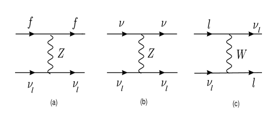
FIG. 2.: Tree-level diagrams for $\nu_{l}f\to\nu_{l}f$ forward scattering; $f$ represents the background fermions. These diagrams are obtained when the corresponding self-energy diagrams [Fig. 1] are cutted along the internal fermion line.

FIG. 3.: Two-loops contributions to the self-energy of a neutrino in a thermal background of charged leptons, nucleons, and neutrinos.