DCPT-02/53

hep-th/0208202

Integrable aspects of the scaling $q$-state Potts models II:
finite-size effects

Patrick Dorey, Andrew Pocklington² and Roberto Tateo

^1,3Dept. of Mathematical Sciences, University of Durham, Durham DH1 3LE, UK

²IFT/UNESP, Instituto de Fisica Teorica, 01405-900, Sao Paulo - SP, Brasil

We continue our discussion of the $q$-state Potts models for $q\leq 4$, in the scaling regimes close to their critical and tricritical points. In a previous paper, the spectrum and full S-matrix of the models on an infinite line were elucidated; here, we consider finite-size behaviour. TBA equations are proposed for all cases related to $\phi_{21}$ and $\phi_{12}$ perturbations of unitary minimal models. These are subjected to a variety of checks in the ultraviolet and infrared limits, and compared with results from a recently-proposed nonlinear integral equation. A nonlinear integral equation is also used to study the flows from tricritical to critical models, over the full range of $q$. Our results should also be of relevance to the study of the off-critical dilute A models in regimes 1 and 2.

1 Introduction

As a second-order phase transition of a lattice model is approached, its correlation length diverges. In the so-called ‘scaling region’ near to the transition, a continuum limit can be taken, and the model can then be investigated using the techniques of continuum field theory. The $q$-state Potts models [1, 2] illustrate this notion very nicely. For $q\leq 4$ the addition of vacancies allows them to be defined so as to have both critical and tricritical points [3], and thus to have two distinct scaling regions, each with its own associated continuum field theory. These are known as the scaling Potts models, with the words critical or tricritical being added if there is a need to be more precise.

This paper is the continuation of a companion paper [4], in which the exact S-matrices of the scaling Potts models were discussed. Our starting-point there was some work by Chim and Zamolodchikov [5], who, noting that the models should be integrable, proposed a set of S-matrix elements describing the scattering of elementary kink-like excitations. Using the bootstrap technique and a ‘minimal’ hypothesis governed by the presence or absence of Coleman-Thun [6] type explanations of S-matrix poles, we were able to close the bootstrap for all of the critical scaling Potts models, and for the tricritical scaling Potts models with $4>q\geq 2$.

The scaling Potts models can be related to $\phi_{21}$ and $\phi_{12}$ perturbations of $c<1$ conformal field theories, and in this context an alternative set of elementary S-matrix elements had previously been proposed by Smirnov [7], using a construction based on reductions of the Izergin-Korepin $a_{2}^{(2)}$ S-matrix [8]. (Interesting features of these scattering theories have recently been discussed in [9, 10].) While the relationship between the two approaches is now being clarified [11], in [4] we found it more convenient to work entirely within Chim and Zamolodchikov’s framework – the fundamental S-matrix elements and the formal vacuum structure are then continuous functions of $q$, and the connection with the Fortuin–Kasteleyn [2] formulation of the lattice model and its symmetries is rather more direct. Smirnov’s approach is perhaps more natural if one wishes to discuss perturbations of specific minimal models, but, as we shall review below, the identification of the scaling Potts models with such perturbations hides a number of subtleties. Nevertheless, it does underline that a study via finite-size effects might be worthwhile, and this topic forms the main theme of the present paper. Taking as partial input the mass spectrum and S-matrix elements found in [4], we propose sets of thermodynamic Bethe ansatz (TBA) equations describing the ground-state energies of the critical and tricritical scaling Potts models, for the values of $q$ for which the associated minimal model is unitary. These proposals are checked in a variety of ways, and we also study aspects of the finite-size behaviour of the models using the so-called non-linear integral equation technique.

The plan of the paper is as follows. Section 2 discusses the conformal field theory descriptions of the critical and tricritical points. Section 3 summarises the necessary S-matrix results obtained in [5] and [4]. Section 4 contains a short review of previous work on the TBA for $\phi_{21}$ and $\phi_{12}$ perturbations, and discusses some features of TBA systems in general. We also sketch some of the reasoning which led to our main conjectures. The conjectures themselves are outlined in sections 5 and 6, in the form of sets of rules for the construction of the eight new families of massive TBA equations for $\phi_{21}$ and $\phi_{12}$ perturbations of the minimal models ${\cal M}_{p,p+1}$, related to the critical and tricritical scaling Potts models at the particular values $\sqrt{q}=2\cos({\textstyle\frac{\pi}{p+1}})$ ($p=6,7,\dots$) and $\sqrt{q}=2\cos({\textstyle\frac{\pi}{p}})$ ($p=5$, $p=7,8,\dots$) respectively. The first four sets of equations for the perturbed critical models are given explicitly in section 5, while the story for the tricritical models is illustrated in section 6 by the set of equations for the ${\cal M}_{5,6}+\phi_{12}$ theory. This is related to the tricritical branch of the Potts model at $\sqrt{q}=2\cos({\textstyle\frac{\pi}{5}})$.

In section 7 our TBA systems are subjected to a number of analytical and numerical tests, all of which they pass. Further verification is provided in section 8, where a variant of the non-linear integral equation of [12] is proposed to describe the finite-size ground-state energy at arbitrary values of $q$ and its solutions are compared numerically with those of the TBA equations. This section also shows how the nonlinear integral equation technique can be used to study the interpolating flows between the tricritical and critical models, by taking an equation first introduced in [13] and tuning its parameters to suitable values.

The full set of TBAs related to both $\phi_{21}$ and $\phi_{12}$ perturbations of minimal unitary models, and the associated sets of functional relations, are given in four appendices.

We end this introduction with a remark on the possible wider relevance of our results. In the following, we have concentrated on the integrable quantum field theories associated to the continuum limits of lattice Potts models near to their critical and tricritical points. A renormalised field theory contains information which is universal in nature, and its relevance is not restricted to any specific member of a universality class. Other lattice systems associated with the “Potts” universality classes are the dilute $A$ models of [14, 15]. While these lattice models are only defined at discrete values of $q$, they have the advantage of being soluble not only at but also away from the critical point, even on the lattice. The link with Potts models comes via the identification of their scaling limits with the $\phi_{12}$ and $\phi_{21}$ perturbations of unitary minimal conformal models. The exact correspondence is [16]:

$$\hbox{Dilute}~{}A_{p-1}\,,~{}\hbox{regime}~{}1^{\pm} \leftrightarrow {\cal M}_{p,p+1}+\phi_{21}~{}\leftrightarrow~{}\sqrt{q}=2\cos({\textstyle\frac{\pi}{p{+}1}})\,,~{}\hbox{critical branch;}$$

$$\hbox{Dilute}~{}A_{p}\,,~{}~{}\hbox{regime}~{}2^{\pm}~{} \leftrightarrow {\cal M}_{p,p+1}+\phi_{12}~{}\leftrightarrow~{}\sqrt{q}=2\cos({\textstyle\frac{\pi}{p}})\,,~{}\hbox{tricritical branch.}$$

These are precisely the points at which we have been able to conjecture TBA descriptions of the continuum models. Past experience (see [17, 18] for examples directly relevant to the matter in hand) suggests a close link between the underlying mathematical structures of the lattice and continuum models, when both are integrable. We therefore expect that many of the results reported in this paper, such as the general forms of the TBAs and the Y-systems, will also play a rôle in the study of the off-critical dilute $A$ models, at least in regimes 1 and 2.

2 The conformal field theory description of the critical and tricritical points

If a model is placed precisely at a second-order transition, its correlation length is infinite and it has no intrinsic length-scale. Its behaviour should therefore be described by a conformal field theory [19]. Some key features of the conformal field theories relevant to the critical $q$-state Potts models with $q\leq 4$ were identified by Dotsenko [20] (see also [21]). His work made use of previous predictions for certain critical exponents of the $q$-state Potts models [22, 23, 24], in particular the following formula, first proposed by den Nijs [22] :

$$y^{\phantom{j_{j}}}_{T}(q)=\frac{6\lambda}{3+2\lambda}\qquad\mbox{where}~{}~{}\sqrt{q}=2\sin\left(\frac{\pi}{3}\lambda\right)~{}~{}\mbox{and}~{}~{}0\leq\lambda\leq 3/2~{}.$$ (2.1)

Here, $y^{\phantom{j_{j}}}_{T}$ is the renormalisation group eigenvalue for the energy operator $\epsilon$ , given in terms of the scaling dimension $x_{\epsilon}$ of $\epsilon$ by $y^{\phantom{j_{j}}}_{T}=2-x_{\epsilon}$ . It is related to the specific heat exponent $\alpha$ as $\alpha=2-2/y_{T}$. (In fact, den Nijs gave his formula in terms of $\mu=\pi/2-\pi\lambda/3$, with $\sqrt{q}=2\cos\mu$, but the parametrisation in terms of $\lambda$ will be more convenient below.)

At the same time, conformal field theories with central charge $c<1$ can be parametrised, at least partially, by a real number $\xi>0$ such that

$$c(\xi)=1-\frac{6}{\xi(\xi{+}1)}~{}.$$ (2.2)

For any (not necessarily rational) value of $\xi$, these theories admit so-called ‘degenerate’ primary fields, which are special in that they have null fields in their sets of descendants, causing their correlation functions to satisfy differential equations [19]. The possible (left) conformal dimensions these fields are

$$\Delta_{r,s}(\xi)=\frac{((\xi{+}1)r-\xi s)^{2}-1}{4\xi(\xi{+}1)}~{}\qquad(r,s\in{\mathbb{N}})\,,$$ (2.3)

with a similar formula for the right conformal dimensions $\bar{\Delta}_{r^{\prime},s^{\prime}}$ . The spinless degenerate primaries have $\Delta=\bar{\Delta}$ so that their scaling dimensions are $x_{r,s}=2\Delta_{r,s}$ ; these fields will be denoted $\phi_{rs}$ .

In [19] and [20], the $2$- and $3$- state Potts models were identified with $c<1$ conformal field theories with $\xi=3$ and $5$ respectively. In both cases, the energy operator $\epsilon$ was shown to correspond to the primary field $\phi_{21}$ . In [20], Dotsenko conjectured that the same should hold for all $q\leq 4$, implying the general relation

$$y^{\phantom{j_{j}}}_{T}(\xi)=2-2\Delta_{2,1}(\xi)=\frac{3(\xi{-}1)}{2\xi}$$ (2.4)

and, comparing with (2.1),

$$\xi=\frac{3+2\lambda}{3-2\lambda}\qquad,\qquad\lambda=\frac{3}{2}\frac{(\xi-1)}{(\xi+1)}~{}.$$ (2.5)

An immediate check on this hypothesis comes via the operator algebra $\phi_{21}\phi_{21}\sim I+\phi_{31}$, which predicts that the critical exponent $y^{\phantom{l}}_{T_{2}}$ (the second thermal exponent) should be given in terms of the scaling dimension $x_{3,1}$ as

$$y^{\phantom{j_{j}}}_{T_{2}}=2-x_{3,1}=-\frac{4}{\xi}=-\frac{4(3-2\lambda)}{(3+2\lambda)}~{}.$$ (2.6)

This matches the value calculated by Nienhuis [23] using a mapping onto a Coulomb gas. Note, since $0\leq\lambda\leq 3/2$ for the Potts models, $\xi$ lies in the range $[1,\infty]$ and $-2\leq c(\xi)\leq 1$.

So far so good; but one should beware that the value of $c$ does not specify a conformal field theory uniquely. Consider the situation when $\xi$ is rational, and suppose that

$$\xi=\frac{p}{p^{\prime}-p}$$ (2.7)

with $p$ and $p^{\prime}$ coprime integers with $p^{\prime}>p$. Then (2.2) and (2.3) turn into the familiar formulae

$$c=1-\frac{6(p^{\prime}-p)^{2}}{pp^{\prime}}~{}~{},\quad\Delta_{r,s}=\frac{(p^{\prime}r-ps)^{2}-(p^{\prime}-p)^{2}}{4pp^{\prime}}$$ (2.8)

and the degenerate fields can be identified in pairs as

$$\phi_{rs}=\phi_{p{-}r,\,p^{\prime}{-}s}~{}.$$ (2.9)

Operator product expansions between fields in the subset

$$\{\phi_{rs}\,|~{}r=1\dots p{-}1,\,s=1\dots p^{\prime}{-}1\}~{},$$ (2.10)

and their descendants, then close amongst themselves. The conformal field theory containing just these fields is called the diagonal, or ‘A’ series, minimal model ${\cal M}_{pp^{\prime}}$ . Depending on the values of $p$ and $p^{\prime}$, there may be other consistent truncations to other field theories also containing finite numbers of degenerate primary fields. All are examples of rational conformal field theories, and the full set of possibilities for $c<1$ forms the famous ADE classification of [25]. However, apart from the special values $\xi=3$ and $5$ (corresponding to $q=2$ and $3$) none of these is the conformal field theory of a $q$-state Potts model. This follows from the fact that the relevant torus partition functions do not coincide [26].

At first sight, this might seem to contradict the claim of [25] to have found a classification of modular invariant partition functions with $c<1$. The Potts model partition functions are certainly modular invariant, so how can they escape this result? The explanation is that the proof in [25] made essential use of the requirement, first emphasised in [27], that all characters should appear in the partition function with non-negative integer multiplicities. This must be true for local quantum field theories whose partition functions can be given as traces of powers of a transfer matrix, but it fails for the Potts models at general values of $q$, for which no such transfer matrix can be defined.

Another way to see the special nature of the Potts conformal field theories is to consider the limit $q\to 4$, or $\xi\to\infty$. To take this limit through minimal models we must send $p,p^{\prime}\rightarrow\infty$, keeping $|p{-}p^{\prime}|$ finite. The scaling dimensions of the degenerate fields tend to $x_{r,s}=(r-s)^{2}/2$, as is reasonable for a theory with $c=1$. However, notice that $x_{r,s}=x_{r+k,s+k}$ for any $k$ . Taking the limit $\xi\to\infty$ through a sequence of minimal models therefore results in a theory in which each scaling dimension appears with an infinite degeneracy. By contrast, the degeneracies of the scaling dimensions in the $4$-state Potts model are finite.

The discussion so far has concentrated on the critical Potts models. For the tricritical models, it turns out that universal quantities are still given by formulae such as (2.1) and (2.2), with the same formula $\sqrt{q}=2\sin(\frac{\pi}{3}\lambda)$ relating $q$ to $\lambda$ or $\xi=(3{+}2\lambda)/(3{-}2\lambda)$, but with $\lambda$ now required to lie in the range $3/2\leq\lambda\leq 3$ [3]. At fixed $q$ this is achieved by sending $\lambda$ to $3-\lambda$, or $\xi$ to $-2-\xi$. Under this continuation, $c(\xi)$ is mapped to $c(\xi{+}1)$, and $\Delta_{21}(\xi)$ to $\Delta_{12}(\xi{+}1)$. This is in accord with the observation of [21], that the exponents for the tricritical models [22, 23] can be recovered by the same style of argument as followed for the critical models, if the energy operator is identified not with $\phi_{21}$, but rather with $\phi_{12}$. However, just as for the critical models, it is only when $q$ is an integer that the partition function of a tricritical Potts model coincides with that of a minimal model.

For both the critical and the tricritical models, the conformal dimension $\Delta$ of the energy operator $\varepsilon$ is

$$\Delta(\lambda)=-\frac{1}{2}+\frac{9}{2(3{+}2\lambda)}~{}.$$ (2.11)

Note that $\Delta(0)=1$, while $\Delta(3)=0$ : the range $[0,3]$ for $\lambda$ is precisely the range for which the energy operator is both relevant and of positive conformal dimension.

We have stressed the fact that the critical and tricritical Potts model partition functions do not generally coincide with those of minimal models, even at points where the central charges match, because a knowledge of the operator content as encoded in the partition function is crucial for the proper interpretation of finite-size effects. Imagine that the theory is defined on a cylinder of circumference $R$. If it is conformal, then the only scale is provided by the system size itself, and so $E(R)$, the ground state energy, must be proportional to $1/R$. The precise relation is [30, 31]

$$E(R)\,=\,-\frac{\pi}{6R}\,c_{\rm eff}$$ (2.12)

where $c_{\rm eff}$, the ‘effective central charge’, is equal to $c-12x_{\rm min}$ , with $x_{\rm min}$ is the smallest scaling dimension in the model. This is the dimension of some field $\phi_{\rm vac}$ which generates the vacuum, or ground, state for the conformal field theory on the cylinder. For a unitary theory, there are no negative-dimension fields and $\phi_{\rm vac}=I$, the identity operator. Thus $x_{\rm min}=0$, and $c_{\rm eff}=c$. However, if the model is non-unitary then negative-dimension operators are to be expected, and as a result $c_{\rm eff}$ is larger than $c$. Whether the Potts models should be considered as unitary or not is perhaps a moot point, but an examination of the partition functions in [26] shows that all the scaling dimensions there are non-negative, and hence, for all $0\leq q\leq 4$, for both the critical and the tricritical models, we have $c_{\rm eff}=c$.

We are interested in the scaling regions around the critical and tricritical points. In the continuum limit, these should be described by perturbed conformal field theories of the form [32]:

$${\cal A}_{q,\tau}={\cal A}_{CFT}+\tau\int\epsilon(x)\,d^{2}x$$ (2.13)

where ${\cal A}_{CFT}$ is the action at the critical or tricritical point, $\tau$ measures the (scaled) deviation from the critical temperature, and the energy density operator $\epsilon(x)$ can be identified with $\phi_{21}(x)$ or $\phi_{12}(x)$ for the critical or tricritical points respectively. The dimensionful coupling $\tau$ introduces an independent length scale $m\propto\tau^{1/(2{-}2\Delta)}$, where $\Delta=\Delta_{21}$ or $\Delta_{12}$ is the conformal dimension of $\epsilon$, given in terms of $\lambda$ by (2.11). The ground state energy $E(R)$ can still be expressed as in (2.12), but now the effective central charge can depend on the dimensionless quantity $r\equiv mR$, and we should also allow for the possibility of a ‘bulk’ term in $E(R)$, proportional to the system size:

$$E(R)\,=\,{\cal E}(\tau)R-\frac{\pi}{6R}\,c(r)\,.$$ (2.14)

The ‘scaling function’ $c(r)$ (for brevity, we shall omit the subscript ‘eff’) encodes a great deal of information about the off-critical model, and will be the main topic of this paper.

3 Mass spectrum and S-matrix data

An important input to our conjectures is the infrared information provided by the mass spectrum and S-matrix of the model on an infinite line. To make this paper relatively self-contained, in this section we summarise the relevant data from [4]. The full spectrum contains both kink and breather states, but since only the diagonal S-matrix elements (those involving at least one breather) enter directly into the TBA systems, only these will be quoted here. The S-matrix elements in §3.2, §3.3 and §3.4 depend on the parameter $\lambda$ introduced in the last section. For rational values of $\lambda$, our results will be equally applicable to perturbations of minimal models ${\cal M}_{p,p^{\prime}}$, modulo the issues of choice of vacuum state $\phi_{\rm vac}$ discussed above. (For the unitary cases $p^{\prime}=p{+}1$ which form the main concern below, the ground states agree and these do not arise anyway.) The relation between $\lambda$ and $p$ and $p^{\prime}$ is

$$\lambda = {\textstyle\frac{3p}{p^{\prime}}}-{\textstyle\frac{3}{2}}~{}~{},~{}~{}~{}(\phi_{21}~{}\mbox{perturbations})$$ (3.1)

$$\lambda = {\textstyle\frac{3p^{\prime}}{p}}-{\textstyle\frac{3}{2}}~{}\,,~{}~{}~{}(\phi_{12}~{}\mbox{perturbations})$$ (3.2)

3.1 Perturbed critical models: $0<\lambda\leq 1$ (one particle)

In this regime there is only the fundamental kink $K\equiv K_{1}$. The physical–strip poles in the kink S-matrix elements at $\theta={\textstyle\frac{2i\pi}{3}}$ and $\theta={\textstyle\frac{i\pi}{3}}$ are due to the fundamental kink itself.

3.2 Perturbed critical models: $1<\lambda<3/2$ (two particles)

A pole at $\theta=i\pi(1{-}1/\lambda)$ enters the physical strip as $\lambda$ passes $1$, and is interpreted as neutral bound state $B\equiv B_{1}$ with mass $m_{B_{1}}=2m_{K}\cos(\frac{\pi}{2}-\frac{\pi}{2\lambda})$. This extra particle brings with it two new scattering amplitudes, ${\cal S}_{B_{1}K_{1}}$ and ${\cal S}_{B_{1}B_{1}}$ :

$${\cal S}_{B_{1}K_{1}} = [\mbox{\footnotesize$\frac{1}{2}$}+\mbox{\footnotesize$\frac{1}{2\lambda}$}][\mbox{\footnotesize$\frac{1}{6}$}+\mbox{\footnotesize$\frac{1}{2\lambda}$}]~{},$$ (3.3)

$${\cal S}_{B_{1}B_{1}} = [\mbox{\footnotesize$\frac{2}{3}$}][\mbox{\footnotesize$\frac{1}{\lambda}$}][\mbox{\footnotesize$\frac{1}{\lambda}$}-\mbox{\footnotesize$\frac{1}{3}$}]~{},$$ (3.4)

where

$$[a]=(a)(1-a)\ \ \ \ \mathrm{and}\ \ \ \ (a)=\frac{\sinh\left(\mbox{\footnotesize$\frac{\theta}{2}$}+\mbox{\footnotesize$\frac{i\pi a}{2}$}\right)}{\sinh\left(\mbox{\footnotesize$\frac{\theta}{2}$}-\mbox{\footnotesize$\frac{i\pi a}{2}$}\right)}~{}.$$ (3.5)

Even though ${\cal S}_{B_{1}K_{1}}$ and ${\cal S}_{B_{1}B_{1}}$ contain further poles, for values of $\lambda$ in this region they can all be explained [4] by invoking a variant of the Coleman-Thun [6, 33] mechanism.

3.3 Perturbed tricritical models: $3/2<\lambda\leq 2$ (four particles)

In addition to $K_{1}$ and $B_{1}$ , two extra particles, a kink $K_{2}$ and a neutral breather $B_{3}$, now enter the spectrum. Their masses are

$$m_{K_{2}}=2m_{K}\cos({\textstyle\frac{\pi}{3}}-{\textstyle\frac{1}{2\lambda}})~{}~{},~{}~{}m_{B_{3}}=2m_{B_{1}}\cos(\mbox{\footnotesize$\frac{\pi}{2\lambda}$}-\mbox{\footnotesize$\frac{\pi}{6}$})~{}~{}\,.$$ (3.6)

No further particles are needed to explain the pole structure up to $\lambda=2$. The new diagonal S-matrix elements are as follows:

$${\cal S}_{B_{1}K_{2}} = [\mbox{\footnotesize$\frac{1}{2}$}][\mbox{\footnotesize$\frac{5}{6}$}][\mbox{\footnotesize$\frac{1}{6}$}+\mbox{\footnotesize$\frac{1}{\lambda}$}][\mbox{\footnotesize$\frac{1}{\lambda}$}-\mbox{\footnotesize$\frac{1}{6}$}]$$

$${\cal S}_{B_{3}K_{1}} = [\mbox{\footnotesize$\frac{1}{3}$}]^{2}[\mbox{\footnotesize$\frac{1}{\lambda}$}][\mbox{\footnotesize$\frac{1}{\lambda}$}+\mbox{\footnotesize$\frac{1}{3}$}]$$

$${\cal S}_{B_{3}K_{2}} = [1-\mbox{\footnotesize$\frac{1}{2\lambda}$}]^{2}[\mbox{\footnotesize$\frac{1}{3}$}+\mbox{\footnotesize$\frac{1}{2\lambda}$}]^{3}[\mbox{\footnotesize$\frac{2}{3}$}+\mbox{\footnotesize$\frac{1}{2\lambda}$}][\mbox{\footnotesize$\frac{3}{2\lambda}$}-\mbox{\footnotesize$\frac{1}{3}$}][\mbox{\footnotesize$\frac{3}{2\lambda}$}]$$

$${\cal S}_{B_{3}B_{3}} = [\mbox{\footnotesize$\frac{2}{3}$}]^{3}[\mbox{\footnotesize$\frac{1}{\lambda}$}]^{3}[\mbox{\footnotesize$\frac{4}{3}$}-\mbox{\footnotesize$\frac{1}{\lambda}$}]^{2}[\mbox{\footnotesize$\frac{1}{3}$}+\mbox{\footnotesize$\frac{1}{\lambda}$}][\mbox{\footnotesize$\frac{2}{\lambda}$}-\mbox{\footnotesize$\frac{2}{3}$}][\mbox{\footnotesize$\frac{2}{\lambda}$}-\mbox{\footnotesize$\frac{1}{3}$}]$$

$${\cal S}_{B_{3}B_{1}} = [\mbox{\footnotesize$\frac{1}{6}$}+\mbox{\footnotesize$\frac{1}{2\lambda}$}]^{2}[\mbox{\footnotesize$\frac{1}{2}$}+\mbox{\footnotesize$\frac{1}{2\lambda}$}][\mbox{\footnotesize$\frac{7}{6}$}-\mbox{\footnotesize$\frac{1}{2\lambda}$}][\mbox{\footnotesize$\frac{3}{2\lambda}$}-\mbox{\footnotesize$\frac{1}{2}$}][\mbox{\footnotesize$\frac{3}{2\lambda}$}-\mbox{\footnotesize$\frac{1}{6}$}]$$ (3.7)

3.4 Perturbed tricritical models: $2<\lambda<9/4$ (six particles)

For $2<\lambda<\frac{9}{4}$ , two more breathers, $B_{2}$ and $B_{5}$, enter the spectrum. The scattering amplitudes for the new particles become increasingly complicated, and greater reliance is placed on the Coleman-Thun mechanism to explain the pole structure. The new S-matrix elements in this region are:

$${\cal S}_{B_{2}B_{1}} = [1-\mbox{\footnotesize$\frac{1}{2\lambda}$}][\mbox{\footnotesize$\frac{2}{3}$}-\mbox{\footnotesize$\frac{1}{2\lambda}$}][\mbox{\footnotesize$\frac{3}{2\lambda}$}][\mbox{\footnotesize$\frac{3}{2\lambda}$}-\mbox{\footnotesize$\frac{1}{3}$}]$$

$${\cal S}_{B_{2}B_{2}} = [\mbox{\footnotesize$\frac{2}{3}$}][\mbox{\footnotesize$\frac{2}{3}$}-\mbox{\footnotesize$\frac{1}{\lambda}$}][\mbox{\footnotesize$\frac{1}{\lambda}$}-\mbox{\footnotesize$\frac{1}{3}$}][\mbox{\footnotesize$\frac{2}{\lambda}$}][\mbox{\footnotesize$\frac{2}{\lambda}$}-\mbox{\footnotesize$\frac{1}{3}$}][1-\mbox{\footnotesize$\frac{1}{\lambda}$}]^{2}$$

$${\cal S}_{B_{2}B_{3}} = [\mbox{\footnotesize$\frac{1}{2}$}][\mbox{\footnotesize$\frac{5}{6}$}][\mbox{\footnotesize$\frac{2}{\lambda}$}-\mbox{\footnotesize$\frac{1}{6}$}][\mbox{\footnotesize$\frac{7}{6}$}-\mbox{\footnotesize$\frac{1}{\lambda}$}]^{2}[\mbox{\footnotesize$\frac{2}{\lambda}$}-\mbox{\footnotesize$\frac{1}{2}$}][\mbox{\footnotesize$\frac{5}{6}$}-\mbox{\footnotesize$\frac{1}{\lambda}$}]^{2}$$

$${\cal S}_{B_{2}K_{1}} = [\mbox{\footnotesize$\frac{1}{2}$}][\mbox{\footnotesize$\frac{1}{6}$}][\mbox{\footnotesize$\frac{1}{2}$}+\mbox{\footnotesize$\frac{1}{\lambda}$}][\mbox{\footnotesize$\frac{1}{6}$}+\mbox{\footnotesize$\frac{1}{\lambda}$}]$$

$${\cal S}_{B_{2}K_{2}} = [\mbox{\footnotesize$\frac{1}{2}$}-\mbox{\footnotesize$\frac{1}{2\lambda}$}]^{2}[\mbox{\footnotesize$\frac{1}{6}$}+\mbox{\footnotesize$\frac{1}{2\lambda}$}]^{2}[\mbox{\footnotesize$\frac{1}{6}$}+\mbox{\footnotesize$\frac{3}{2\lambda}$}][\mbox{\footnotesize$\frac{3}{2\lambda}$}-\mbox{\footnotesize$\frac{1}{6}$}]$$

$${\cal S}_{B_{5}B_{1}} = [\mbox{\footnotesize$\frac{1}{3}$}]^{2}[\mbox{\footnotesize$\frac{4}{3}$}-\mbox{\footnotesize$\frac{1}{\lambda}$}][\mbox{\footnotesize$\frac{1}{3}$}+\mbox{\footnotesize$\frac{1}{\lambda}$}][\mbox{\footnotesize$\frac{2}{\lambda}$}-\mbox{\footnotesize$\frac{2}{3}$}][\mbox{\footnotesize$\frac{2}{\lambda}$}-\mbox{\footnotesize$\frac{1}{3}$}][1-\mbox{\footnotesize$\frac{1}{\lambda}$}]^{2}$$

$${\cal S}_{B_{5}B_{2}} = [\mbox{\footnotesize$\frac{4}{3}$}-\mbox{\footnotesize$\frac{3}{2\lambda}$}]^{2}[1-\mbox{\footnotesize$\frac{3}{2\lambda}$}]^{2}[\mbox{\footnotesize$\frac{2}{3}$}+\mbox{\footnotesize$\frac{1}{2\lambda}$}][\mbox{\footnotesize$\frac{1}{3}$}+\mbox{\footnotesize$\frac{1}{2\lambda}$}]^{3}[1-\mbox{\footnotesize$\frac{1}{2\lambda}$}]^{2}[\mbox{\footnotesize$\frac{5}{2\lambda}$}-\mbox{\footnotesize$\frac{1}{3}$}][\mbox{\footnotesize$\frac{5}{2\lambda}$}-\mbox{\footnotesize$\frac{2}{3}$}]$$

$${\cal S}_{B_{5}B_{3}} = [\mbox{\footnotesize$\frac{7}{6}$}-\mbox{\footnotesize$\frac{1}{2\lambda}$}][\mbox{\footnotesize$\frac{1}{6}$}+\mbox{\footnotesize$\frac{3}{2\lambda}$}][\mbox{\footnotesize$\frac{3}{2}$}-\mbox{\footnotesize$\frac{3}{2\lambda}$}]^{2}[\mbox{\footnotesize$\frac{5}{2\lambda}$}-\mbox{\footnotesize$\frac{5}{6}$}][\mbox{\footnotesize$\frac{1}{2}$}+\mbox{\footnotesize$\frac{1}{2\lambda}$}]^{3}[\mbox{\footnotesize$\frac{3}{2\lambda}$}-\mbox{\footnotesize$\frac{1}{6}$}]^{3}[\mbox{\footnotesize$\frac{5}{2\lambda}$}-\mbox{\footnotesize$\frac{1}{2}$}][\mbox{\footnotesize$\frac{5}{6}$}-\mbox{\footnotesize$\frac{1}{2\lambda}$}]^{4}$$

$${\cal S}_{B_{5}B_{5}} = [\mbox{\footnotesize$\frac{5}{3}$}-\mbox{\footnotesize$\frac{2}{\lambda}$}]^{2}[\mbox{\footnotesize$\frac{2}{3}$}]^{5}[\mbox{\footnotesize$\frac{3}{\lambda}$}-1][\mbox{\footnotesize$\frac{3}{\lambda}$}-\mbox{\footnotesize$\frac{2}{3}$}][\mbox{\footnotesize$\frac{1}{\lambda}$}]^{5}[\mbox{\footnotesize$\frac{1}{3}$}+\mbox{\footnotesize$\frac{1}{\lambda}$}]^{3}[\mbox{\footnotesize$\frac{4}{3}$}-\mbox{\footnotesize$\frac{2}{\lambda}$}]^{3}[\mbox{\footnotesize$\frac{2}{\lambda}$}][\mbox{\footnotesize$\frac{4}{3}$}-\mbox{\footnotesize$\frac{1}{\lambda}$}]^{2}$$

$${\cal S}_{B_{5}K_{1}} = [\mbox{\footnotesize$\frac{1}{2}$}-\mbox{\footnotesize$\frac{1}{2\lambda}$}]^{2}[\mbox{\footnotesize$\frac{5}{6}$}-\mbox{\footnotesize$\frac{1}{2\lambda}$}]^{2}[\mbox{\footnotesize$\frac{1}{6}$}+\mbox{\footnotesize$\frac{3}{2\lambda}$}][\mbox{\footnotesize$\frac{3}{2\lambda}$}-\mbox{\footnotesize$\frac{1}{6}$}]$$

$${\cal S}_{B_{5}K_{2}} = [\mbox{\footnotesize$\frac{5}{6}$}]^{2}[\mbox{\footnotesize$\frac{1}{2}$}]^{2}[\mbox{\footnotesize$\frac{7}{6}$}-\mbox{\footnotesize$\frac{1}{\lambda}$}]^{2}[\mbox{\footnotesize$\frac{5}{6}$}-\mbox{\footnotesize$\frac{1}{\lambda}$}]^{3}[\mbox{\footnotesize$\frac{1}{2}$}+\mbox{\footnotesize$\frac{1}{\lambda}$}][\mbox{\footnotesize$\frac{2}{\lambda}$}-\mbox{\footnotesize$\frac{1}{6}$}][\mbox{\footnotesize$\frac{2}{\lambda}$}-\mbox{\footnotesize$\frac{1}{2}$}]$$ (3.8)

The complete mass spectrum up to $\lambda=9/4$ is:

$$\begin{array}[]{ll}m_{K_{1}}=m{}&(\lambda>0)\\[3.0pt] m_{B_{1}}=2m\cos(\mbox{\footnotesize$\frac{\pi}{2}$}-\mbox{\footnotesize$\frac{\pi}{2\lambda}$}){}&(\lambda>1)\\[3.0pt] m_{K_{2}}=2m\cos(\mbox{\footnotesize$\frac{\pi}{3}$}-\mbox{\footnotesize$\frac{\pi}{2\lambda}$}){}&(\lambda>3/2)\\[3.0pt] m_{B_{3}}=4m\cos(\mbox{\footnotesize$\frac{\pi}{2}$}-\mbox{\footnotesize$\frac{\pi}{2\lambda}$})\cos(\mbox{\footnotesize$\frac{\pi}{2\lambda}$}-\mbox{\footnotesize$\frac{\pi}{6}$}){}&(\lambda>3/2)\\[3.0pt] m_{B_{2}}=2m\cos(\mbox{\footnotesize$\frac{\pi}{2}$}-\mbox{\footnotesize$\frac{\pi}{\lambda}$}){}&(\lambda>2)\\[3.0pt] m_{B_{5}}=4m\sin(\mbox{\footnotesize$\frac{\pi}{\lambda}$})\cos(\mbox{\footnotesize$\frac{\pi}{3}$}-\mbox{\footnotesize$\frac{\pi}{2\lambda}$}){}&(\lambda>2)\end{array}$$

4 The thermodynamic Bethe ansatz

Our aim is to probe the models (2.13) via their properties in finite spatial volumes. The main tool will be the thermodynamic Bethe ansatz (TBA) approach, a technique which allows the finite-size ground state energy of a theory to be obtained via the solution of a collection of coupled nonlinear integral equations.

If the set of TBA equations is to be finite, then we would expect that the unperturbed theory should be associated with a minimal model in some way (as recalled above, for non-integer values of $q$ the critical or tricritical $q$-state Potts model is never precisely the same as a minimal model, but the operator subalgebras generated by the energy operator agree, and so the ground-state energies based on the ‘conformal’ vacuum state $I$ should coincide.) The precise form of the equations will depend on the particular model being perturbed, and only a limited number of cases have been studied to date. Before describing our new conjectures, we shall give a brief summary of the earlier work.

4.1 Earlier work

The situation is summarised in table 1; the cited papers can be consulted for further explanations. Many of these results can, sometimes with hindsight, be labelled according to the ‘$g\diamond g^{\prime}$’ scheme put forward in [42], where $g$ and $g^{\prime}$ indicate a pair of diagrams of ADET type. Since the $A_{1}$ incidence matrix is zero, the TBA for the $A_{1}\diamond A_{1}$ case is trivial, reflecting the fact that the field theory of ${\cal M}_{3,4}+\phi_{13}$, the thermally-perturbed Ising model, is free. Two other cases, labelled $(G_{2})$ and $(F_{4})$, also have a Lie-algebraic interpretation, though the fact that these algebras are not simply-laced places them outside the set of $g\diamond g^{\prime}$ systems. However, their form is in line with a more general set of Lie algebraic TBA systems discussed in [43, 44]. As was remarked in [4], there is an intriguing coincidence between the sequence $\{A_{1},A_{2},G_{2},D_{4},F_{4},E_{6},E_{6},E_{7},E_{8}\}$ which arises naturally in connection with the Potts models, and the ‘exceptional series’ of Lie algebras making up the last line of the extended Freudenthal magic square, as discussed by Deligne, Cohen and de Man, Cvitanovic and others [45, 46, 47, 48, 49]. In [47], Deligne and de Man identified an extra member of the series, namely the superalgebra $OSp(1|2)$. From our point of view this corresponds to ${\cal M}_{7,10}+\phi_{21}$, where the unperturbed CFT is the $OSp(1|2)^{(1)}\times OSp(1|2)^{(1)}/OSp(1|2)^{(2)}$ coset conformal field theory [4]. The relevant TBA is the $T_{1}\diamond D_{3}$ system, the $n=3$ case of the third line of table 1.

However, it is important to realise that all of the infinite sets of systems listed in table 1 describe the ground states of perturbations of non-unitary minimal models, generated by negative-dimension operators and not the identity. These TBAs are therefore not directly relevant for the $q$-state Potts models, although one might hope that the addition of a suitable chemical potential would allow them to describe the Potts vacuum state as well (see for example [50, 51, 34]). We will not discuss this possibility any further here, but it would be an interesting avenue to explore.

Minimal	Perturbing	$\lambda$	$c$	$c_{\rm eff}(0)$	$\phi_{\rm vac}$	TBA	Ref.
model	field					system
${\cal M}_{n,2n-1}$	$\phi_{21}$	$\frac{3}{4n{-}2}$	$-\mbox{\footnotesize$\frac{(n-2)(4n-3)}{n(2n-1)}$}$	$\frac{(n-2)(2n+3)}{n(2n-1)}$	$\phi_{12}$	$T_{1}\diamond A_{2n-4}\!$	[34, 35]
${\cal M}_{2n+1,4n}$	$\phi_{21}$	$\frac{3}{4n}$	$-\mbox{\footnotesize$\frac{(2n-3)(4n-1)}{2n(2n+1)}$}$	$\frac{4n^{2}+2n-3}{2n(2n+1)}$	$\phi_{n,2n-1}$	$T_{1}\diamond T_{2n-1}$	[36]
${\cal M}_{2n+1,4n-2}\!$	$\phi_{21}$	$\frac{3}{2n-1}$	$-\mbox{\footnotesize$\frac{4(n-1)(2n-7)}{(2n-1)(2n+1)}$}$	$\frac{4n^{2}-4}{4n^{2}-1}$	$\phi_{\left[\mbox{\footnotesize$\frac{n+1}{2}$}\right],2\left[\mbox{\footnotesize$\frac{n+1}{2}$}\right]-1}\!$	$T_{1}\diamond D_{n}$	[37]
${\cal M}_{3,4}$	$\phi_{21}({=}\phi_{13})$	$\frac{3}{4}$	$\frac{1}{2}$	$\frac{1}{2}$	$\phi_{11}$	$A_{1}\diamond A_{1}$
${\cal M}_{4,5}$	$\phi_{21}$	$\frac{9}{10}$	$\frac{7}{10}$	$\frac{7}{10}$	$\phi_{11}$		[35]
${\cal M}_{5,6}$	$\phi_{21}$	$1$	$\frac{4}{5}$	$\frac{4}{5}$	$\phi_{11}$	$A_{2}\diamond A_{1}$	[38]
${\cal M}_{9,10}$	$\phi_{21}$	$\frac{6}{5}$	$\frac{14}{15}$	$\frac{14}{15}$	$\phi_{11}$	$(G_{2})$	[39]
$(c=1)$	$\phi_{21}{=}\phi_{12}$	$\frac{3}{2}$	$1$	$1$	$I$	$D_{4}\diamond A_{1}$	[40]
${\cal M}_{10,11}$	$\phi_{12}$	$\frac{9}{5}$	$\frac{52}{55}$	$\frac{52}{55}$	$\phi_{11}$	$(F_{4})$	[39]
${\cal M}_{6,7}$	$\phi_{12}$	$2$	$\frac{6}{7}$	$\frac{6}{7}$	$\phi_{11}$	$E_{6}\diamond A_{1}$	[40]
${\cal M}_{4,5}$	$\phi_{12}$	$\frac{9}{4}$	$\frac{7}{10}$	$\frac{7}{10}$	$\phi_{11}$	$E_{7}\diamond A_{1}$	[40]
${\cal M}_{3,4}$	$\phi_{12}$	$\frac{5}{2}$	$\frac{1}{2}$	$\frac{1}{2}$	$\phi_{11}$	$E_{8}\diamond A_{1}$	[40]
${\cal M}_{2,5}$	$\phi_{12}$	$6$	$-\mbox{\footnotesize$\frac{22}{5}$}$	$\frac{2}{5}$	$\phi_{12}$	$T_{1}\diamond A_{1}$	[38]
${\cal M}_{2,2n+1}$	$\phi_{12}$	$3n$	$-\mbox{\footnotesize$\frac{2(n-1)(6n-1)}{2n+1}$}$	$\frac{2n-2}{2n+1}$	$\phi_{1n}$		[41]

Table 1: TBA systems for minimal models perturbed by $\phi_{21}$ and $\phi_{12}$. For the systems of $g\diamond g^{\prime}$ type, the mass in the magnonic system should be placed on the first node (that furthest from the tadpole or fork for $T_{n}$ or $D_{n}$). $[x]$ is the integer part of $x$.

The observation that a TBA system related to $G_{2}$ might describe the $\phi_{21}$ perturbation of ${\cal M}_{9,10}$ ($\lambda=\frac{6}{5}$) was made in [39]. This point lies in the region where the analysis of [4] suggests two particle types in the model, and indeed that is precisely what the TBA system of [39] predicts. This case will be discussed along with the new TBA systems below, and for now we merely stress that, just as for almost all the above examples, this TBA system was first obtained as a conjecture, only subsequently being checked to describe the claimed model.

A more deductive approach can be found in a paper by Bazhanov and Ellem [35], who discussed the $\phi_{21}$ perturbations of ${\cal M}_{4,5}$ ($\lambda=\frac{9}{10}$) and ${\cal M}_{3,5}$ ($\lambda=\frac{3}{10}$), taking Smirnov’s RSOS description of the massive scattering theories [7] as their starting-point. Subject to some mild assumptions, they derived sets of TBA equations for these two cases. Crucial was the fact [52] that for these models the RSOS restriction on the allowed vacuum states coincides with the restriction imposed on adjacent spins in the hard hexagon model [53]. Unfortunately this equivalence holds only for a subset of the whole family of models related to $a_{2}^{(2)}$ (as mentioned in [35], another example, to which we shall return in §6 below, is the theory ${\cal M}_{5,6}+\phi_{12}$). Thus, the extension of the approach of [35] to further models faces considerable obstacles.

One other piece of work should be mentioned at this stage, even though its ultimate conclusions appear to run counter to the findings that will be reported below. In the course of a detailed study of character and polynomial identities associated with general $\phi_{21}$ perturbations, Berkovich, McCoy and Pearce [54] discussed possible TBA equations for all unitary minimal models ${\cal M}_{p,p+1}$, which reduced to the result of [35] for $p=4$. They were only able to specify the general form of these equations, and certain (‘kernel’) functions necessary for a complete conjecture were left undetermined. Nevertheless, at least on a naïve reading, the equations of [54] appear to entail just a single massive kink in the model for all values of $p$. This is at variance with the results of [4], which for $\phi_{21}$ perturbations predict that there should be a kink and a breather for all $p>5$. In later sections we shall propose some new TBA systems which are consistent with this spectrum. There may be room to accommodate both our results and those of [54] – the closing remarks of [55] indicate one possibility – but we suspect that the final resolution will reside in some modification to the considerations of [54] to bring their TBA systems into line with ours, at least insofar as they concern $\phi_{21}$ perturbations of unitary minimal models.

For now we shall leave this question unresolved, and proceed with a discussion of the general form that we would expect the TBA equations to take, assuming for the time being that the results of [4] do indeed provide a reliable guide.

4.2 The general structure of TBA systems

When all scattering is diagonal, the integral equations of the TBA follow directly from the bulk S-matrix. The ground state energy of the model on a circle of circumference $R$ is written in terms of ‘dressed’ single-particle energies $\varepsilon_{a}(\theta)$ (pseudoenergies)[38]. These pseudoenergies solve a system of non-linear integral equations of the following form:

$$\varepsilon_{a}(\theta)=Rm_{a}\cosh\theta-\sum_{c=1}^{N}\Phi_{ac}*L_{c}(\theta)\,.$$ (4.1)

Here $L_{c}(\theta)=\ln(1+e^{-\varepsilon_{c}(\theta)}),$ $*$ denotes the convolution

$$f*g(\theta)={1\over 2\pi}\int_{-\infty}^{\infty}f(\theta^{\prime})g(\theta-\theta^{\prime})d\theta^{\prime}\,,$$ (4.2)

and the $2\to 2$ S-matrix elements ${\cal S}_{ac}(\theta)$ influence the equations through the kernel functions $\Phi_{ac}(\theta)$:

$$\Phi_{ac}(\theta)=-i{d\over d\theta}\ln{\cal S}_{ac}(\theta)\,.$$ (4.3)

The number of pseudoenergies coincides with the number $N$ of particle types in the original scattering theory. From (4.1), they have the large $\theta$ asymptotics

$$\varepsilon_{a}(\theta)|_{\theta\rightarrow\infty}\sim Rm_{a}\cosh\theta~{}~{},~{}~{}(a=1,2,\dots,N~{}).$$ (4.4)

If off-diagonal scattering is also involved the complexity of the method increases significantly, as it is necessary to perform an extra ‘diagonalisation’ step before the final equations can be written down (see, for example, [35] for further discussion of this point). But once the dust has settled, one generally finds that the parts of the TBA equations associated with diagonal scattering are as before, while the contribution of each kink multiplet $K$ is split into two parts. The first is described by a single pseudoenergy $\varepsilon_{K}(\theta)$ with an asymptotic of the type (4.4), with $m_{K}$ the common mass of all kinks in the multiplet. In addition, diagonalisation results in the introduction of a (possibly infinite) number of auxiliary pseudoenergies. These behave as

$$\varepsilon_{a}(\theta)|_{\theta\rightarrow\infty}\sim\mbox{constant}~{}~{},~{}~{}a=N+1,N+2,\dots~{}~{},$$ (4.5)

and can be associated with fictitious ‘particles’ transporting zero energy and zero momentum (note that $m_{a}\cosh\theta$ in (4.4) is the single-particle energy on the infinite line). These new particles are often called ‘magnons’, and can be thought of as constructs introduced to get the counting of states right. The diagonalisation is by no means trivial, and in the following we will instead make a conjecture, using the above considerations as our guide and borrowing elements from some previously encountered TBA systems.

4.3 The steps towards the main conjectures

Our TBA conjectures were found via a link with the TBA equations for perturbed ${\mathbb{Z}}_{N}$ systems of [56]. Originally this emerged from a study of four previously-known $\phi_{12}$-related cases. These were: ${\cal M}_{3,4}+\phi_{12}$ (related to $E_{8}$), ${\cal M}_{4,5}+\phi_{12}$ (related to $E_{7}$), ${\cal M}_{6,7}+\phi_{12}$ (related to $E_{6}$) and ${\cal M}_{10,11}+\phi_{12}$ (related to $F_{4}$). No hint of a common structure came by just looking at the first three models, but a consideration of ${\cal M}_{6,7}+\phi_{12}$ and ${\cal M}_{10,11}+\phi_{12}$ alone revealed some striking analogies with systems related to $a_{1}^{(1)}$. To see this, let us compare them with the sine-Gordon TBAs at ${\textstyle\frac{\beta^{2}}{8\pi}}={\textstyle\frac{1}{4}}$ and ${\textstyle\frac{\beta^{2}}{8\pi}}={\textstyle\frac{2}{7}}$. The four systems are depicted in figures 4.3, 4.3, 4.3 and 4.3. (Figure 4.3 is the $E_{6}$-related system: the distinction between solitons and antisolitons is special to this, the case of the tricritical Potts model, and so the $E_{6}$ diagram symmetry has been used to superimpose each pair of soliton-antisoliton nodes, resulting in the diagram shown. Likewise, figure 4.3 is the $D_{4}$-related point of the sine-Gordon model, and the $D_{4}$ diagram symmetry has been used to superimpose the soliton and the antisoliton.) There is a formal similarity between the pairs of diagrams in figures 4.3 and 4.3 and in figures 4.3 and 4.3, the main differences being related to the fact that there is just a single soliton-antisoliton pair in the sine-Gordon model, and correspondingly just a single massive ‘soliton’ node in the $a_{1}^{(1)}$-related TBA systems.

$$\begin{array}[]{cc}\epsfbox[00288338]{d40.eps}&\epsfbox[00288338]{e6.eps}\\[5.0pt] \parbox[t]{216.81pt}{\small\raggedright Figure \ref{f1.a}: Sine-Gordon TBA at ${\textstyle\frac{\beta^{2}}{8\pi}}={\textstyle\frac{1}{4}}$ \@add@raggedright}&\parbox[t]{147.4292pt}{\small\raggedright Figure \ref{f1.b}: ${\cal M}_{6,7}+\phi_{12}$\@add@raggedright}\\[-30.0pt] \epsfbox[00288350]{d41.eps}&\epsfbox[00288350]{f4.eps}\\[5.0pt] \parbox[t]{216.81pt}{\small\raggedright Figure \ref{f2.a}: Sine-Gordon TBA at ${\textstyle\frac{\beta^{2}}{8\pi}}={\textstyle\frac{2}{7}}$ \@add@raggedright}&\parbox[t]{147.4292pt}{\small\raggedright Figure \ref{f2.b}: ${\cal M}_{10,11}+\phi_{12}$ \@add@raggedright}\\[30.0pt] \epsfbox[00288350]{d4g.eps}&\epsfbox[00288350]{f4g.eps}\\[5.0pt] \parbox[t]{216.81pt}{\small\raggedright Figure \ref{f3.a}: Sine-Gordon TBA at ${\textstyle\frac{\beta^{2}}{8\pi}}={\textstyle\frac{n-1}{3n-2}}$ \@add@raggedright}&\parbox[t]{147.4292pt}{\small\raggedright Figure \ref{f3.b}: ${\cal M}_{4n+6,4n+7}+\phi_{12}$ \@add@raggedright}\end{array}$$

The sine-Gordon TBA systems of figures 4.3 and 4.3 are the first members of a series of models at ${\textstyle\frac{\beta^{2}}{8\pi}}={\textstyle\frac{n-1}{3n-2}}$, represented in figure 4.3, which have an $A_{1}\diamond D_{n-1}$ magnonic structure. This fact made it natural to generalise the ${\cal M}_{6,7}+\phi_{12}$ and ${\cal M}_{10,11}+\phi_{12}$ TBA systems in a similar manner, by ‘nesting’ an $A_{2}\diamond D_{n-1}$ magnonic system on top of the two $a_{2}^{(2)}$ soliton nodes. Graphically the result is shown in figure 4.3.

Working first at the level of associated sets of functional equations called Y-systems, checks on periodicities and central charges were used to fix the details. We finally converged to the proposal of appendix B.2 (Case $\widetilde{D}$), which covers the family of models ${\cal M}_{4n+6,4n+7}+\phi_{12}$. This gave a clear signal that the general $\phi_{12}$ perturbations of unitary minimal models share the ‘modulo 4’ property of the ${\mathbb{Z}}_{N}$-related systems found in [56], an observation which enabled us to obtain the remaining cases by replacing the $A_{2}\diamond D_{n-1}$ part with the other families of systems from [56]. Full TBA equations were then obtained by Fourier transforming the Y-systems.

Once it was seen that the systems in [56] were playing a central rôle, it was possible, following similar reasoning, to conjecture the TBAs for the $\phi_{21}$ perturbations. In these cases elements of the S-matrix were first used to fix the ‘diagonal’ part of the TBA equations, with the systems of ref. [56] then being adapted to describe the magnonic part. The Y-systems were then derived by using standard methods, paying attention to the pole structure of the kernel functions (see appendix A.1 and, for example, [42]). As should be clear from this discussion, the process was one of educated guesswork; however the detailed checks that we report below leave us in no doubt that the final systems are correct.

5 TBA conjectures: $\phi_{21}$ perturbations of unitary minimal models

In this section we shall be concerned with thermal perturbations of critical Potts models at points where the central charges of the unperturbed models coincide with those of the unitary minimal models ${\cal M}_{p,p+1}$, $p\geq 3$, which means that we set $\sqrt{q}=2\cos\frac{\pi}{(p{+}1)}$ , and $\lambda=\frac{3}{2}(p{-}1)/(p{+}1)$ , $\xi=p$ . As explained earlier, the fact that the related minimal models are unitary means that we will equally be describing the behaviour of the ground states of perturbations of minimal models, the perturbing operator being $\phi_{21}$ in all cases.

For $p=3$, $4$ and $5$, $\lambda\leq 1$ and the spectrum consists of the fundamental kink alone. TBA systems are already known for these cases – the first is the (trivial) example of the thermally-perturbed Ising model, the second was treated in [35], and the third is the thermally-perturbed 3-state Potts model, for which the TBA was written in [38]. Therefore we will suppose that $p\geq 6$, which ensures that the bulk spectrum has one kink, and one breather [4]. The form of the ‘non-magnonic’ part of the TBA is then fixed almost completely by the results of §3:

$$\varepsilon_{B}(\theta) = Rm_{B}\cosh\theta-\sum_{c\in\{B,K\}}\Phi_{Bc}*L_{c}(\theta)~{},$$

$$\varepsilon_{K}(\theta) = Rm_{K}\cosh\theta-\sum_{c\in\{B,K\}}\Phi_{Kc}*L_{c}(\theta)+(\hbox{magnonic terms})~{},$$ (5.1)

with the effective central charge given by

$$c(r)={3\over\pi^{2}}\sum_{c\in\{B,K\}}\int_{-\infty}^{\infty}d\theta~{}m_{c}R~{}\cosh\theta L_{c}(\theta){}~{}~{}~{},~{}~{}~{}(r=m_{K}R)~{}.$$ (5.2)

The kernel functions involving diagonal S-matrix elements are:

$$\Phi_{BB}(\theta)=-i{d\over d\theta}\ln{\cal S}_{BB}(\theta){}~{}~{}~{}~{},~{}~{}~{}~{}\Phi_{KB}(\theta)=\Phi_{BK}(\theta)=-i{d\over d\theta}\ln{\cal S}_{KB}(\theta)~{}.$$ (5.3)

The last term in (5.1) indicates the presence of the extra contributions from the as-yet unknown number of magnons. In addition, equations involving magnons and kink pseudoenergies are required. It is at this stage that our conjectures begin, with most of the deduction proceeding, as explained in the last section, by analogy with the models studied in [39, 56]. We start with the kernel $\Phi_{KK}(\theta)$. Since the scattering of two kinks is not generally diagonal, this is not expected to be a simple logarithmic derivative of an S-matrix element. However, if we set

$$\rho=\left({1\over 2}-{1\over 2\lambda}\right)~{},$$ (5.4)

then we observe that the mass relation

$$m_{B}=2\cos(\pi\rho)m_{K}$$ (5.5)

is accompanied by the following S-matrix identity:

$${\cal S}_{aB}(\theta)={\cal S}_{aK}(\theta+i{\pi\rho}){\cal S}_{aK}(\theta-i{\pi\rho})~{}~{},~{}~{}~{}(a=B)$$ (5.6)

or, equivalently

$$\Phi_{aB}(\theta)=\Phi_{aK}(\theta+i\pi\rho)+\Phi_{aK}(\theta-i\pi\rho)~{}~{},~{}~{}~{}(\theta\neq 0,a=B)~{}.$$ (5.7)

The constraint $\theta\neq 0$ is due to the fact that $\Phi_{BK}(\theta)$ has poles at $\theta=\pm i\pi\rho$. Care is needed when the identity is integrated, either in Fourier transforms or in convolutions. Relations between the kernels such as (5.5) and (5.7), involving every pair of particle species, are needed in order to convert a TBA equation into a Y-system, and so we shall assume that (5.7) holds for $a=K$ too. Assuming also that $\Phi_{KK}(\theta)$ is free of singularities in the strip $|\Im m\theta|\leq\pi\rho$, we obtain

$$\Phi_{KK}(\theta)=\chi_{\rho}*\Phi_{KB}(\theta)~{}~{},~{}~{}\chi_{\rho}(\theta)={1\over 2\rho\cosh(\theta/2\rho)}~{}.$$ (5.8)

For the reasons outlined in the last section, we looked to the TBA systems which had previously arisen in the context of self-dual perturbations of ${\mathbb{Z}}_{N}$-symmetric conformal field theories for the remaining equations. It turns out that for the $\phi_{21}$ perturbations of the unitary minimal models ${\cal M}_{p,p+1}$ with $p>5$, the equations proposed in [56] can be adapted to provide an appropriate set of ‘magnonic’ equations. The equations in [56] were obtained via a ‘doubling’ of the sine-Gordon TBA systems at certain special points $\beta^{2}=32\pi/N$, $\xi=1/(N/4-1)$.

The recipe goes as follows. Consider first the continued-fraction expansion of

$${6\rho}=\left({p-5\over p-1}\right)~{}.$$ (5.9)

For the unitary models ${\cal M}_{p,p+1}$ this results in four families of cases:

$$A)~{}~{}~{}p=4n+2~{}~{}:~{}~{}{6\rho} = {1\over 1+{1\over{n-1+{1\over 4}}}}$$

$$B)~{}~{}~{}p=4n+3~{}~{}:~{}~{}{6\rho} = {1\over 1+{1\over{n-1+{1\over 2}}}}$$

$$C)~{}~{}~{}p=4n+4~{}~{}:~{}~{}{6\rho} = {1\over 1+{1\over{n-1+{1\over{1+{1\over 3}}}}}}$$ (5.10)

$$D)~{}~{}~{}p=4n+5~{}~{}:~{}~{}{6\rho} = {1\over 1+{1\over n}}$$

matching the four families of cases seen in [56]. The second ‘nested’ continued-fraction decomposition of $6\rho$ in (5.10), i.e. the decomposition of $\rho_{2}=1/(6\rho)-1$, matches the special values $\xi=1/(N/4-1)$ observed in connection with the ${\mathbb{Z}}_{N}$ models, if we identify $N=p-1$. The fact that the match is at a nested level reflects the idea that these extra pseudoenergies are supposed to be of magnonic type, and for this reason we also trade the driving terms of [56] for

$$\nu_{j}^{(\alpha)}(\theta)=\delta_{\alpha 1}\psi_{1j}*L_{K}(\theta)~{}~{},$$ (5.11)

and set

$$(\mbox{magnonic terms})=\sum_{j}\psi_{1j}*L^{(1)}_{j}(\theta)\,,$$ (5.12)

where $j=1,\dots,n$ for cases A, B and C and $j=1,\dots,n+1$ for case D. Finally, the variables $\theta$, $\theta^{\prime}$ used in [56] should be rescaled. This can again be interpreted as a consequence of the fact that the match is at a nested level and the rôle of $1/h=2/(N-4)$ of [56] is now played by the quantity $1/g=\rho\rho_{2}=4\rho/(p-5)=2\rho/h$ (i.e. $g=3(p-1)/2$). This is equivalent to a replacing the kernels $\phi_{ij}^{[{\mathbb{Z}}_{N}]}(\theta)$ , $\psi_{ij}^{[{\mathbb{Z}}_{N}]}(\theta)$ and $\phi_{k}^{[{\mathbb{Z}}_{N}]}(\theta)$ defined in appendix A of [56] with

$$\phi_{ij}(\theta)={1\over 2\rho}\phi_{ij}^{[{\mathbb{Z}}_{N}]}({\theta\over 2\rho})~{}~{},~{}~{}\psi_{ij}(\theta)={1\over 2\rho}\psi_{ij}^{[{\mathbb{Z}}_{N}]}({\theta\over 2\rho})~{}~{},~{}~{}\phi_{k}(\theta)={1\over 2\rho}\phi_{k}^{[{\mathbb{Z}}_{N}]}({\theta\over 2\rho})~{}~{}.$$ (5.14)

In appendix A the resulting set of TBA equations is written explicitly, while in §7 we report some analytical and numerical evidence for their correctness.

Before that, we will give the explicit forms of the TBA systems for the first four cases, $p=6,7,8,9$. These are the first unitary models for which the extra particle $B\equiv B_{1}$ is expected to appear, and at the same time their magnonic structures are still relatively simple. In each case, the TBA system is conjectured to describe the perturbation of ${\cal M}_{p,p{+}1}$ by $\phi_{21}$.

A) ${\bf p=6}$ (n=1, $\lambda={15\over 14}$):

$$\varepsilon_{B}(\theta) = Rm_{B}\cosh\theta-\sum_{c\in\{B,K\}}\Phi_{Bc}*L_{c}(\theta)$$

$$\varepsilon_{K}(\theta) = Rm_{K}\cosh\theta-\sum_{c\in\{B,K\}}\Phi_{Kc}*L_{c}(\theta)-\phi_{2}*L^{(1)}(\theta)$$

$$\varepsilon^{(\gamma)}(\theta) = -\sum_{\beta=1}^{6}l^{[E_{6}]}_{\gamma\beta}\phi_{2}*L^{(\beta)}(\theta)-\delta_{\gamma 1}\phi_{2}*L_{K}(\theta)~{}~{}~{}~{}(\gamma=1,\dots,6)$$ (5.15)

In this case there are six magnons and $l^{[E_{6}]}_{\alpha\beta}$ is the incidence matrix of the $E_{6}$ Dynkin diagram with nodes labelled as in figure 5.

B) ${\bf p=7}$ (n=1, $\lambda={9\over 8}$):

$$\varepsilon_{B}(\theta) = Rm_{B}\cosh\theta-\sum_{c\in\{B,K\}}\Phi_{Bc}*L_{c}(\theta)$$

$$\varepsilon_{K}(\theta) = Rm_{K}\cosh\theta-\sum_{c\in\{B,K\}}\Phi_{Kc}*L_{c}(\theta)-\phi_{1}*L^{(1)}(\theta)$$

$$\varepsilon^{(\gamma)}(\theta) = -\sum_{\beta=0}^{4}l^{[A_{5}]}_{\gamma\beta}\phi_{1}*L^{(\beta)}(\theta)-\delta_{\gamma 1}\phi_{1}*L_{K}(\theta)~{}~{}~{}~{}~{}(\gamma=0,\dots,4)$$ (5.16)

Here, there are five auxiliary pseudoenergies and $l^{[A_{5}]}_{\gamma\beta}$ is the incidence matrix of the $A_{5}$ Dynkin diagram with nodes labelled as in figure 5.

C) ${\bf p=8}$ (n=1, $\lambda={7\over 6}$):

$$\varepsilon_{B}(\theta) = Rm_{B}\cosh\theta-\sum_{c\in\{B,K\}}\Phi_{Bc}*L_{c}(\theta)$$

$$\varepsilon_{K}(\theta) = Rm_{K}\cosh\theta-\sum_{c\in\{B,K\}}\Phi_{Kc}*L_{c}(\theta)-\phi_{3}*L^{(1)}(\theta)$$

$$\varepsilon^{(1)}(\theta) = -\phi_{3}*(L_{K}(\theta)+L^{(6)}(\theta)+L^{(4)}(\theta))-\phi_{4}*L^{(3)}(\theta)-\phi_{5}*L^{(5)}(\theta)$$

$$\varepsilon^{(3)}(\theta) = \phi_{2}*(K^{(5)}(\theta)-L^{(1)}(\theta))$$

$$\varepsilon^{(5)}(\theta) = \phi_{2}*(K^{(3)}(\theta)+K^{(6)}(\theta)+K^{(4)}(\theta))$$

$$\varepsilon^{(6)}(\theta) = \phi_{2}*K^{(5)}(\theta)$$

$$\varepsilon^{(4)}(\theta) = \phi_{2}*(K^{(5)}(\theta)-L^{(2)}(\theta))$$

$$\varepsilon^{(2)}(\theta) = -\phi_{3}*(L^{(6)}(\theta)+L^{(3)}(\theta))-\phi_{4}*L^{(4)}(\theta)-\phi_{5}*L^{(5)}(\theta)$$ (5.17)

where $K^{(c)}(\theta)=\ln(1+e^{\varepsilon^{(c)}(\theta)})$ .

D) ${\bf p=9}$ (n=1, $\lambda={6\over 5}$):

$$\varepsilon_{B}(\theta) = Rm_{B}\cosh\theta-\sum_{c\in\{B,K\}}\Phi_{Bc}*L_{c}(\theta)$$

$$\varepsilon_{K}(\theta) = Rm_{K}\cosh\theta-\sum_{c\in\{B,K\}}\Phi_{Kc}*L_{c}(\theta)+\psi*\left(L^{(1)}(\theta)+L^{(3)}(\theta)\right)$$

$$\varepsilon^{(\gamma)}(\theta) = \sum_{\beta=1}^{2}l^{[A_{2}]}_{\gamma\beta}\psi*L^{(\beta)}(\theta)+\delta_{\gamma 1}\psi*L_{K}(\theta)~{}~{}~{}~{}~{}~{}~{}(\gamma=1,2)$$

$$\varepsilon^{(\gamma)}(\theta) = \sum_{\beta=3}^{4}l^{[A_{2}]}_{\gamma\beta}\psi*L^{(\beta)}(\theta)+\delta_{\gamma 3}\psi*L_{K}(\theta)~{}~{}~{}~{}~{}~{}~{}(\gamma=3,4)$$ (5.18)

where $\psi(\theta)\equiv\psi_{11}(\theta)=\psi_{22}(\theta)$. In this case there are four auxiliary pseudoenergies and $l^{[A_{2}]}_{\alpha\beta}$ is the incidence matrix of the $A_{2}$ Dynkin diagram with nodes labelled as in figure 5. It was noted in [39] that this TBA can be mapped into a particular case of the $G_{2}$-related Y-systems of [43]. Notice also that the pseudoparticle part factorises into a pair of $A_{2}$-type TBAs while a single one was found for the model ${\cal M}_{4,5}$ studied in [35]. This can be explained by observing that the vacuum incidence diagram ($k=8$ in [60]) is (orbifold) equivalent to the product of two “hard hexagon” diagrams ($k=3$ in [60]). Thus also in this case a simple variant of the analysis of [35] should lead to a more rigorous derivation of the system, though this remains to be done.

$$\begin{array}[]{cc}\epsfbox[050288338]{NM67.eps}&\epsfbox[050288338]{NM78.eps}\\ {}\hfil\\ {}\hfil\\ {}\hfil\\ \parbox[t]{151.76964pt}{\small\raggedright Figure \ref{figure9.a}: ${\cal M}_{6,7}+\phi_{21}$ \@add@raggedright}&\parbox[t]{151.76964pt}{\small\raggedright Figure \ref{figure9.b}: ${\cal M}_{7,8}+\phi_{21}$ \@add@raggedright}\end{array}$$

$$\begin{array}[]{cc}\epsfbox[050288350]{NM89.eps}&\epsfbox[050288350]{NM910.eps}\\ {}\hfil\\ {}\hfil\\ {}\hfil\\ \parbox[t]{151.76964pt}{\small\raggedright Figure \ref{figure9.c}: ${\cal M}_{8,9}+\phi_{21}$ \@add@raggedright}&\parbox[t]{151.76964pt}{\small\raggedright Figure \ref{figure9.d}: ${\cal M}_{9,10}+\phi_{21}$ \@add@raggedright}\end{array}$$

6 TBA conjectures: $\lambda>3/2$

We were also able to construct the TBA equations describing the ground-state energies of the unitary ${\cal M}_{p,p+1}+\phi_{12}$ models. As in the cases related to $\phi_{21}$ , we split the set of unitary minimal models into four families, which we label $\widetilde{A}\dots\widetilde{D}$. For $p\geq 7$, the spectrum consists of just four particles (two neutral particles $B_{1}$ and $B_{3}$ and two kinks $K_{1}$ and $K_{2}$). Here the magnonic sector resembles again the ${\mathbb{Z}}_{N}$-related structure described in [56]. A pictorial representation of the TBA systems for the family ${\cal M}_{4n+3,4n+4}$ is given in figure 11. Note that at $n=0$, what for $n>0$ had been a magnonic $E_{6}$-type sector in the TBA naturally generates the extra six neutral particles needed to reconstruct the full $E_{8}$-related mass spectrum of the $\phi_{12}$-perturbed Ising model.

Figure 11: Diagrammatic representation for the ${\cal M}_{4n+3,4n+4}+\phi_{12}$ TBA systems

The full sets of TBA equations and Y-systems are given in appendix B.

We shall illustrate these proposals with the simplest new system, corresponding to the model ${\cal M}_{5,6}+\phi_{12}$. For this case, $\lambda={\textstyle\frac{21}{10}}$ and so, referring back to §3, we expect the spectrum to contain six particles, $B_{1}$, $B_{2}$, $B_{3}$, $B_{5}$, $K_{1}$ and $K_{2}$. In addition, we conjecture that two magnonic pseudoenergies, $\varepsilon^{(1)}$ and $\varepsilon^{(2)}$, should be introduced to deal with the non-diagonal nature of the kink scattering. The equations are:

$$\varepsilon_{b}(\theta) = Rm_{b}\cosh\theta-\sum_{c}\Phi_{bc}*L_{c}(\theta)-(\delta_{b,K_{1}}+\delta_{b,K_{2}})\phi*L^{(1)}(\theta)$$

$$\varepsilon^{(1)}(\theta) = -\phi*(L^{(2)}(\theta)+L_{K_{1}}(\theta)+L_{K_{2}}(\theta))$$ (6.1)

$$\varepsilon^{(2)}(\theta) = -\phi*L^{(1)}(\theta)$$

with $b,c\in\{B_{1},B_{2},B_{3},B_{5},K_{1},K_{2}\}$. The kernels are:

$$\Phi_{bb^{\prime}}(\theta)=-i{d\over d\theta}\ln{\cal S}_{bb^{\prime}}(\theta){}~{}~{}~{}~{},~{}~{}~{}~{}\Phi_{kb}(\theta)=\Phi_{bk}(\theta)=-i{d\over d\theta}\ln{\cal S}_{kb}(\theta)$$ (6.2)

where $b,b^{\prime}\in\{B_{1},B_{2},B_{3},B_{5}\}$, $k\in\{K_{1},K_{2}\}$ and

$$\Phi_{K_{1}K_{1}}(\theta)=\phi*\Phi_{K_{1}B_{2}}(\theta){}~{}~{},~{}~{}\Phi_{K_{2}K_{2}}(\theta)=\phi*\Phi_{K_{2}B_{5}}(\theta)\,,$$ (6.3)

$$\Phi_{K_{1}K_{2}}(\theta)=\Phi_{K_{2}K_{1}}(\theta)=\phi*\Phi_{B_{5}K_{1}}(\theta){}~{}~{},~{}~{}\phi(\theta)=\frac{21}{\cosh(21\,\theta)}\,.$$ (6.4)

A diagrammatic representation is shown in figure 12.

Figure 12: Diagrammatic representation for the ${\cal M}_{5,6}+\phi_{12}$ TBA system

Again the $A_{2}$-type pseudoparticle sector reflects the relationship between this theory and the hard hexagon model [35].

7 Analytical and numerical checks

This section gathers together some evidence, analytical and numerical, in favour of the conjectured TBA systems. The value of the UV central charge is obtained through standard manipulations of the TBA equations [38, 40], which allow $c_{\mbox{\tiny UV}}\equiv c(0)$ to be expressed as a sum of Rogers dilogarithm functions. The arguments of the dilogarithms are expressed in terms of the set of stationary solutions of the TBA at $r=0$ and $r=\infty$. We did not recognise these sums among any of the standard relations for the Rogers function (see for example [61]), so we relied on numerical work to check that, up to $p=13$ and to about $15$ digit accuracy, we have the expected result

$$c_{\mbox{\tiny UV}}\equiv c(0)=1-{6\over p(p+1)}~{}.$$ (7.1)

Next, we discuss the corrections to $c(0)$ which make up the UV expansion of $c(r)$. A key idea is to find a set of functional relations satisfied by the exponentiated pseudoenergies, called a Y-system. These generally imply a periodicity property for the pseudoenergies under a certain imaginary shift in $\theta$, which in turn can be used to deduce information about the $r$-dependence of $c(r)$. This phenomenon was first noticed by Al.B. Zamolodchikov in [62], for Y-systems related to the TBA equations described in  [40] and encoded by a single ADE Dynkin diagram. (The periodicity for the A and D cases was subsequently proved in [63, 64, 65], while a general proof also covering the E cases was only given recently, in [66].)

The Y-systems pertinent to $\phi_{21}$ perturbations are collected together in appendix A. We did not attempt to prove their periodicity properties, but numerically verified the following result:

$$Y_{a}(\theta+i\pi P)=Y_{a}(\theta),~{}~{}~{}~{}P={8p\over 6(p-1)}$$ (7.2)

Following the arguments of [62], periodicity implies an expansion for $c(r)$ in powers of $r^{4/P}$ and fixes the dimension of an odd perturbing operator to

$$\bar{\Delta}=\Delta=1-{1\over P}={p+3\over 4p}\,.$$ (7.3)

This value coincides with the conformal dimension of the operator $\phi_{21}$.

A numerical study of $c(r)$ for the $\phi_{21}$ TBA systems also indicates the presence of a single irregular ‘anti-bulk’ term:

$$c(r)=c-{\cal B}\,r^{2}+\sum_{n=1}^{\infty}c_{n}r^{n(3p-3)/p}\,.$$ (7.4)

This term is related to the bulk free energy of (2.14) by ${\cal B}=-6{\cal E}/(\pi m_{K}^{2})$ ; it can be calculated analytically from the TBA by adapting the method of [38, 40]. For $\theta\rightarrow-\infty$ we have

$$\Phi_{ab}(\theta)\sim-\Phi_{BB}^{(1)}\left({m_{a}\over m_{B}}\right)\left({m_{b}\over m_{B}}\right)e^{\theta}+\dots~{},~{}~{}~{}(a,b\in\{B,K\})\,,$$ (7.5)

with

$$\Phi_{BB}^{(1)}=4\left(\sin(\frac{2\pi}{3})+\sin(\frac{\pi}{\lambda})+\sin(\frac{\pi}{\lambda}-\frac{\pi}{3})\right)\,.$$ (7.6)

Arguing as in [38, 40], we therefore have

$${\cal B}={3\over\pi\Phi_{BB}^{(1)}}\left({m_{B}\over m_{K}}\right)^{2}=\frac{\sqrt{3}\,}{2\pi}\,\frac{\sin({\pi\over 3}{p+1\over p-1})}{\sin({2\pi\over 3}{p\over p-1})}~{}~{}.$$ (7.7)

This matches the result given in [67].

Next, the coefficients $c_{n}$ in the expansion (7.4) can be checked against the results of conformal perturbation theory (CPT). This predicts an expansion

$$c_{\scriptstyle\rm{CPT}}(r)\equiv-{6R\over\pi}E(\tau,R)={c}+\sum_{m=2}^{\infty}B_{m}t^{m}~{}~{},~{}~{}t=-\pi\tau(R/2\pi)^{2-2\Delta}\,,$$ (7.8)

which should match (7.4) save for the absence of the anti-bulk term $-{\cal B}\,r^{2}$. The CPT coefficients $B_{m}$ are given in terms of connected correlation functions on the plane. For unitary cases,

$$B_{m}={24\over\pi^{m-1}m!}\int\langle\varepsilon(1,1)\varepsilon(z_{1},\bar{z}_{1})\dots\varepsilon(z_{m-1},\bar{z}_{m-1})\rangle_{c}\prod_{k=1}^{m-1}{d^{2}z_{k}\over(z_{k}\bar{z}_{k})^{1-\Delta}}~{},$$ (7.9)

with conformal invariance fixing

$$B_{2}=12{\gamma^{2}(\Delta)\over\gamma(2\Delta)}~{}~{},~{}~{}\gamma(x)={\Gamma(x)\over\Gamma(1-x)}~{}.$$ (7.10)

The high-low temperature duality symmetry of the model is reflected in the fact that correlators with an odd number of $\varepsilon$ operators vanish identically ($B_{m}=0$ for odd $m$). Comparing (7.4) with (7.8) confirms that our effective central charge behaves as that of a minimal conformal field theory perturbed by $\phi_{21}$ ($\bar{\Delta}_{21}=\Delta_{21}={p+3\over 4p}$). On dimensional grounds there must be a relation between $\tau$ and $m_{K}$ (the mass of the kink $K\equiv K_{1}$ appearing in (5.1) and (5.2)) of the form $\tau=\kappa m_{K}^{2-2\Delta}$, where $\kappa$ is a dimensionless constant whose exact value was calculated by other methods in [67]. Table 2 compares numerical results from the TBA with the exact formula.

Model	$\kappa^{2}$  (TBA)	$\kappa^{2}$  (Exact)
${\cal M}_{6,7}+\phi_{21}$	0.0259899061737	0.02598990617395
${\cal M}_{7,8}+\phi_{21}$	0.02506361950681	0.02506361950686
${\cal M}_{8,9}+\phi_{21}$	0.0242806346097	0.02428063460990
${\cal M}_{9,10}+\phi_{21}$	0.02362954340274	0.02362954340277

Table 2: TBA data versus the exact results of [67]

Similar checks can be performed for the $\phi_{12}$ perturbations. The relevant functional relations are given in appendix B, and we verified that in these cases the periodicities implied by the Y-systems are $P=\frac{8(p+1)}{6(p+2)}\,$. The resulting conformal dimensions $(p-2)/(4p+4)$ match those of the $\phi_{12}$ operator.

Finally, we turn to the large-$R$ behaviour, restricting attention to the $\phi_{21}$ systems for brevity. The system (5.1) implies the following asymptotic for the ground-state energy $E(m_{K},R)$:

$$E(m_{K},R)=-{\pi\over 6R}c(r)\sim{\sigma m_{K}\pi}K_{1}(r)\,,$$ (7.11)

where $\sigma$ can be evaluated in terms of the quantities $\Upsilon_{i}^{(1)}$ in appendix C of [56]. Setting $\eta=\pi/(p+1)$ and $n=\mbox{Int}[(p-2)/4]$ we have

$$\sigma = \left(1+{1\over\Upsilon^{(1)}_{n}}\right)^{\!1/2}\,\prod_{i=1}^{n-1}\left(1+{1\over\Upsilon_{i}^{(1)}}\right)$$ (7.12)

$$= \left(1+{\sin(2\eta)\sin((2n+2)\eta)\over\sin^{2}(n\eta)}\right)^{\!1/2}\,\prod_{i=1}^{n-1}\left(1+{\sin(2\eta)\sin(\eta)\over\sin((i+3)\eta)\sin(i\eta)}\right)$$

$$= 4\cos^{2}\eta-1=q-1$$

for cases A,B and C and

$$\sigma = \left(1+{1\over\Upsilon_{n}^{(1)}}\right)^{\!1/2}\,\left(1+{1\over\Upsilon_{n+1}^{(1)}}\right)^{\!1/2}\,\prod_{i=1}^{n-1}\left(1+{1\over\Upsilon_{i}^{(1)}}\right)$$ (7.13)

$$= \left(1+{2\sin(\eta)\cos((n+1)\eta)\over\sin(n\eta)}\right)\prod_{i=1}^{n-1}\left(1+{\sin(2\eta)\sin(\eta)\over\sin((i+3)\eta)\sin(i\eta)}\right)$$

$$= 4\cos^{2}\eta-1=q-1$$

for case D. The value $\sigma=q-1$ matches the prediction of an argument given in [56], extending the instanton ideas of [68, 69], that $\sigma$ should be the Perron-Frobenius eigenvalue of the (in this case $S_{q}$-symmetric) incidence matrix $I^{(q)}_{ab}$ encoding the number of light kinks which join each pair of vacua. Note that the argument is a little formal here, since in general the number of vacua is not an integer. For these unitary cases this worry can be averted by shifting to the RSOS approach of [7]; either way, the TBA systems meet our expectations.

8 Results from the nonlinear integral equation approach

The TBA is not the only exact technique on the market for the study of finite-size effects. Another class of methods is known as the nonlinear integral equation (NLIE) approach. These equations generally depend smoothly on their parameters, and so are in some senses better-suited to a description of the $q$-state Potts models. The downside is that the full particle content is encoded in a much more implicit way, and so they have less to say on the issues of bootstrap closure discussed in [4].

8.1 Massive flows

A non-linear integral equation describing general $\phi_{12}$, $\phi_{21}$ and $\phi_{15}$ perturbations within a unified framework was proposed in [12], similar in spirit to the equations related to $\phi_{13}$ perturbations introduced in [70, 71]. In contrast to the TBA equations discussed earlier, in [12] the set of pseudoenergies $\{\,\varepsilon_{a}\,\}$ is traded for a single unknown function $f(\theta)$, which solves the following equation:

$$f(\theta)=i\pi\alpha-ir\sinh\theta+\!\int_{{\cal C}_{1}}\!\!\varphi(\theta{-}\theta^{\prime})\ln(1{+}e^{f(\theta^{\prime})})\,d\theta^{\prime}-\!\int_{{\cal C}_{2}}\!\!\varphi(\theta{-}\theta^{\prime})\ln(1{+}e^{-f(\theta^{\prime})})\,d\theta^{\prime}\,,$$ (8.1)

where $r=m_{K}R$ with $m_{K}$ the mass of the fundamental kink. Given $f(\theta)$, the effective central charge can be evaluated as

$$c_{\rm eff}(r)={3ir\over\pi^{2}}\left(\int_{{\cal C}_{1}}\sinh\theta\,\ln(1{+}e^{f(\theta)})\,d\theta-\int_{{\cal C}_{2}}\sinh\theta\,\ln(1{+}e^{-f(\theta)})\,d\theta\right)\,.$$ (8.2)

The contours ${\cal C}_{1}$ and ${\cal C}_{2}$ run from $-\infty$ to $+\infty$, just below and just above the real $\theta$-axis, and the kernel $\varphi(\theta)$ depends continuously on the parameter $\lambda$ as

$$\varphi(\theta)=-\int_{-\infty}^{\infty}\frac{e^{ik\theta}\sinh({\textstyle\frac{\pi}{3}}k)\cosh({\textstyle\frac{\pi}{6}}(1{-}{\textstyle\frac{3}{\lambda}})k)}{\cosh({\textstyle\frac{\pi}{2}}k)\sinh({\textstyle\frac{\pi}{2\lambda}}k)}\frac{dk}{2\pi}=-\frac{i}{2\pi}\frac{d}{d\theta}\log\,S(\theta)~{}.$$ (8.3)

As before, $\sqrt{q}=2\sin({\textstyle\frac{\pi}{3}}\lambda)$ , while $S(\theta)$ is the scalar part of the fundamental kink-kink scattering amplitudes as given in [4]. (A scale-invariant version of this system had previously appeared in the context of lattice models; see [72].) In [12], we showed how to use (8.1) to describe perturbations of unitary and non-unitary minimal models, tuning the twist parameter $\alpha$ so as to account for the fact that the ground state may be generated by a negative-dimension field. For current purposes, we are more interested the $q$-state Potts models and their tricritical variants, for which, as discussed earlier, the ground state always comes from the identity operator. For these theories, $\alpha$ should be related to $\lambda$ as

$$\alpha=\frac{2\lambda}{3}-1\,.$$ (8.4)

The reader should note that the NLIE (8.2) is simpler and, not being restricted to special points, of wider applicability than the TBA equations proposed in §5 and §6 above. It is also much more appropriate for discussions of the $q\to 1$ limit relevant to percolation. However, it does not encode, in any direct way, information about the bound-state content of the associated field theory.

In Table 3 we compare results from the NLIE and TBA approaches. The agreement is very good, ranging from 10 to 14 significant digits.

Model	$r$	TBA	NLIE
${\cal M}_{10,11}+\phi_{21}$	0.2	0.9328551607515	0.9328551607514
	0.3	0.9185246910885	0.9185246910884
${\cal M}_{11,12}+\phi_{21}$	0.2	0.9421554960427	0.9421554960424
	0.3	0.9279952931412	0.9279952931410
${\cal M}_{12,13}+\phi_{21}$	0.2	0.949321521251	0.949321521253
	0.3	0.935305379646	0.935305379648
${\cal M}_{13,14}+\phi_{21}$	0.2	0.954961250612733	0.954961250612730
	0.3	0.941068318324234	0.941068318324237
${\cal M}_{5,6}+\phi_{12}$	0.2	0.79241547642	0.79241547640
	0.3	0.78313881742	0.78313881742

Table 3: Comparison between TBA and the NLIE proposed in  [12]

8.2 Massless flows from tricritical to critical models

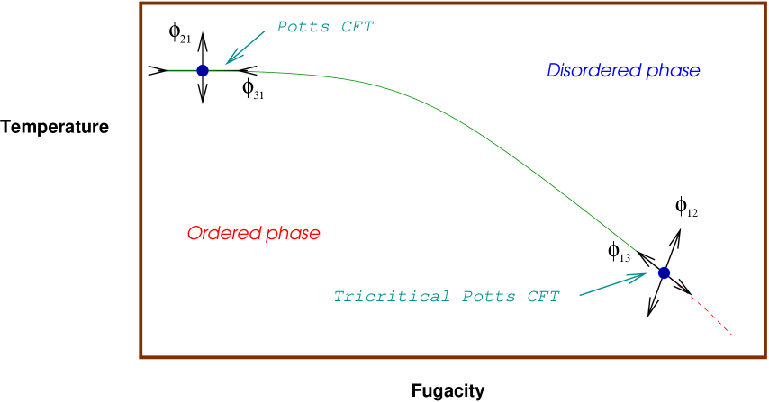
Figure 13: The phase diagram

In addition to the perturbations discussed so far, the concentration of vacancies in a tricritical Potts model can be adjusted so as to drive the theory either onto a line of first-order transitions, or else down via a massless flow to the corresponding critical model. The relevant operator turns out to be $\phi_{13}$, which is always in the spectrum of the tricritical models. The full picture is illustrated in figure 13; it is most convenient to use the parameter $\xi$ for these flows, related to $q$ by $\sqrt{q}=2\cos\pi/(\xi{+}1)$ with $\xi\in[1,\infty]$. The massless flow is then

$$c_{\rm tricrit}(\xi)=1-\frac{6}{(\xi+1)(\xi+2)}~{}~{}~{}\to~{}~{}~{}c_{\rm crit}(\xi)=1-\frac{6}{\xi(\xi+1)}~{}.$$ (8.5)

For $\xi=p\in{\mathbb{Z}}$, this is the well-known massless $\phi_{13}$ flow from ${\cal M}_{p{+}1,p{+}2}$ to ${\cal M}_{p,p{+}1}$ [73, 74] for which equations of TBA type were proposed in [75]. To describe the flows at general values of $\xi$, we instead adapt an equation proposed by Zamolodchikov in [13] for the study of flows in the imaginary-coupled sine-Gordon model from $c=1$ to $c=1$. In [37], it was shown that the twist parameters in Zamolodchikov’s equation could be chosen so as to describe flows between both unitary and non-unitary minimal models, revealing a striking non-monotonicity of $c(r)$ at intermediate scales in the non-unitary cases. Here, we shall propose a further modification to capture the general flows between tricritical and critical Potts models. As in [13], introduce two analytic functions $f_{R}(\theta)$ and $f_{L}(\theta)$, and couple them together via

$$f_{R}(\theta) = -i\frac{r}{2}e^{\theta}+i\pi\alpha^{\prime}$$

$$+\int_{{\cal C}_{1}}\!\phi(\theta-\theta^{\prime})\ln(1+e^{f_{R}(\theta^{\prime})})~{}d\theta^{\prime}-\int_{{\cal C}_{2}}\!\phi(\theta-\theta^{\prime})\ln(1+e^{-f_{R}(\theta^{\prime})})~{}d\theta^{\prime}$$

$$+\int_{{\cal C}_{1}}\!\chi(\theta-\theta^{\prime})\ln(1+e^{-f_{L}(\theta^{\prime})})~{}d\theta^{\prime}-\int_{{\cal C}_{2}}\!\chi(\theta-\theta^{\prime})\ln(1+e^{f_{L}(\theta^{\prime})})~{}d\theta^{\prime}\quad$$

$$f_{L}(\theta) = -i\frac{r}{2}e^{-\theta}-i\pi\alpha^{\prime}$$ (8.6)

$$+\int_{{\cal C}_{2}}\!\phi(\theta-\theta^{\prime})\ln(1+e^{f_{L}(\theta^{\prime})})~{}d\theta^{\prime}-\int_{{\cal C}_{1}}\!\phi(\theta-\theta^{\prime})\ln(1+e^{-f_{L}(\theta^{\prime})})~{}d\theta^{\prime}$$

$$+\int_{{\cal C}_{2}}\!\chi(\theta-\theta^{\prime})\ln(1+e^{-f_{R}(\theta^{\prime})})~{}d\theta^{\prime}-\int_{{\cal C}_{1}}\!\chi(\theta-\theta^{\prime})\ln(1+e^{f_{R}(\theta^{\prime})})~{}d\theta^{\prime}\quad$$

where

$$\phi(\theta)=\int_{-\infty}^{\infty}\frac{e^{ik\theta}\sinh(k(\xi-1){\textstyle\frac{\pi}{2}})}{2\cosh({\textstyle\frac{\pi}{2}}k)\sinh(k{\textstyle\frac{\pi}{2}}\xi)}\frac{dk}{2\pi}~{},$$ (8.7)

$$\chi(\theta)={-}\int_{-\infty}^{\infty}\frac{e^{ik\theta}\sinh({\textstyle\frac{\pi k}{2}})}{2\cosh({\textstyle\frac{\pi k}{2}})\sinh({\textstyle\frac{\pi k}{2}}\xi)}\frac{dk}{2\pi}~{}.$$ (8.8)

(In [13] , the kernels were given in terms of a parameter $p\equiv\xi{+}1$ .) We have $\sqrt{q}=2\cos\pi/(\xi{+}1)$ with $\xi\in[1,\infty]$, and, for the interpolating Potts flows, $\alpha^{\prime}$ must be chosen as

$$\alpha^{\prime}={1\over\xi}~{}.$$ (8.9)

In terms of the solutions to these equations, the effective central charge is

$$c_{\rm eff}(r) = \frac{3ir}{2\pi^{2}}\biggl{[}\int_{{\cal C}_{1}}\!\!e^{\theta}\ln(1{+}e^{f_{R}(\theta)})\,d\theta-\int_{{\cal C}_{2}}\!\!e^{\theta}\ln(1{+}e^{-f_{R}(\theta)})\,d\theta$$ (8.10)

$${}~{}~{}~{}{}+\int_{{\cal C}_{2}}\!\!e^{-\theta}\ln(1{+}e^{f_{L}(\theta)})\,d\theta-\int_{{\cal C}_{1}}\!\!e^{-\theta}\ln(1{+}e^{-f_{L}(\theta)})\,d\theta\biggr{]}~{}.$$

$$\begin{array}[]{c}\includegraphics[width=346.89731pt]{cplot.eps}\end{array}$$

Figure 14: Flows of $c(r)$ as obtained from the NLIE (8.6), plotted against $\log(r/2)$. Highlighted are the flows from $c=1/2$ to $c=0$ and from $c=0$ to $c=-2$.

Figure 14 shows our numerical results. As long as the IR destination has a positive central charge, the flows are monotonic, even at points corresponding to non-unitary minimal models. This is in sharp contrast to the behaviour of the $\phi_{13}$-perturbed minimal models themselves, for which a number of non-monotonic flows of $c(r)$ were exhibited in [37]. To some extent, this reflects the already-mentioned fact that the ground states of Potts and minimal models do not coincide away from unitary points, but it is nonetheless surprising that the switch to the identity vacuum state manages to eliminate all of the non-monotonicity while $c_{IR}$ remains positive.

The other notable feature of figure 14 is the behaviour of the flow from $c=0$ to $c=-2$, which exhibits a cusp, suggestive of a level-crossing, at an intermediate length-scale. In fact, this curve deserves a second glance for another reason: in [76], Fendley, Saleur and Zamolodchikov pointed out that the effective central charge along this particular flow should be protected by supersymmetry, at least for small enough values of $r$, and hence should be identically zero. They also, by an indirect argument, predicted that this picture would be changed by a level-crossing at $r\approx 2.95708396$. The apparent contradiction of their first claim with our results has a neat resolution: one has to remember that, just as for the TBA equations discussed earlier, the quantity $c(r)$ produced by the NLIE includes an ‘anti-bulk’ piece, non-analytic in the coupling constant, which ensures that at large values of $r$, $c(r)$ tends to a constant. Thus, just as in equations (7.4) and (7.8) above, we expect

$$c(r)=c_{\mbox{\tiny CPT}}(r)-{\cal B}\,r^{2}$$ (8.11)

where $c_{\mbox{\tiny CPT}}(r)$ is the physical, unsubtracted quantity, while $c(r)$ is the quantity which is found directly from the NLIE. The ‘Bulk’ constant ${\cal B}$ was found exactly in [77] by considering a related theory in a magnetic field; it can also be obtained directly from equations (8.6) and (8.10), using an argument described for a similar equation in [56]. Either way, the answer is

$${\cal B}=-\frac{3}{2\pi}\frac{1}{\cos(\frac{\pi}{2}(\xi{+}1))}~{}.$$ (8.12)

Specialising to $\xi=1$, we see that before the bottom curve of figure 14 is compared with the proposals of [76], the quantity $\frac{3}{2\pi}r^{2}$ should be added to it. Numerically, it is hard to do this directly due to instabilities in the equations near $\xi=1$, so in figure 15 we show a sequence of plots of the appropriately-adjusted functions $c_{\mbox{\tiny CPT}}(r)=c(r)+{\cal B}(\xi)r^{2}$, for $\xi=1.03$ down to $\xi=1.005$, together with an extrapolated curve for $\xi=1$. (For the extrapolation, numerical data down to $\xi=1.001$ was used.) Not only does the revised curve meet general supersymmetric expectations; the point at which supersymmetry was predicted in [76] to be spontaneously broken via a level-crossing is also reproduced. We suspect that there is more to be said on this matter, and the nice agreement between our results and those of [76] certainly deserves to be understood at a deeper and more analytical level. For now, we leave this for future investigations.

$$\begin{array}[]{c}\includegraphics[angle={270},width=303.53267pt]{cplot2.eps}\end{array}$$

Figure 15: Flows of $c_{\mbox{\tiny CPT}}(r)$ for $\xi=1.03,1.025,\dots 1.005$ as obtained from the NLIE, plotted against $\log(r/2)$. Also shown is the extrapolated curve for $\xi=1$ (dotted), and the location of the level-crossing predicted in [76].

9 Conclusions

In the past decade there has been a common belief that $A_{n}$–, $D_{n}$– and $E_{n}$– related integrable systems should exhibit a certain uniformity of structure. As we remarked in [4], the bulk, S-matrix, description of the real-coupling simply-laced affine Toda field theories (and their minimal variants) illustrate this philosophy well: all the scattering data can be encoded using the root systems of the associated Lie algebras [78]. A first sign of a breakdown in this pattern in other contexts came with the attempt to make the coupling imaginary in these same Toda models: the $A_{1}$ Toda Hamiltonian remains Hermitian, turning into the sine-Gordon Hamiltonian, while all the others become complex. Despite this crucial difference, it was initially thought that the relatively simple $A_{1}$-related sine-Gordon spectrum might be the first instance of some unified description valid for all Lie algebras [79, 80]. Smirnov’s work [7] had already suggested that matters were likely to be much more complicated, and subsequent work, in particular [81] and [4], has confirmed this expectation, to the extent that there is still no complete understanding of the bulk scattering theory associated with any imaginary-coupled Toda theory beyond the $A_{1}$ case.

On side of lattice models and the Bethe ansatz, a longstanding hope has been to find generalisations of the construction of Takahashi and Suzuki [58], who many years ago found the correct ‘string hypothesis’ describing the Bethe ansatz solutions relevant to the finite volume corrections-to-scaling of the $XXZ$ model at arbitrary values of the anisotropy. The form taken by the Bethe ansatz equations for this model are the $A_{1}$ cases of a general set of ADE-related Bethe ansatz equations, given just in terms of Lie algebra parameters in [82]. The symmetry of equations in nature is often broken by their solutions, and for three decades all attempts to generalise the construction by Takahashi and Suzuki to the other lattice models at arbitrary values of the coupling constant have failed. (The difficulties even for the $SU(3)$ case were highlighted in [81].)

Building on a relationship with the $q$-state Potts models, in this paper we have conjectured and checked TBA equations related to $a_{2}^{(2)}$ at points related to the unitary series of minimal models perturbed by their $\phi_{21}$ and $\phi_{12}$ operators. Although we have proposed a continued-fraction decomposition, a la Takahashi-Suzuki, that governs these systems, we are currently unable to extend the analysis to the other rational points. Yet, the models described, being unitary, are physically the most interesting, and we hope that our work will motivate a more rigorous derivation of these equations. In this respect we feel that the functional approach described in, for example, [83, 84], and already applied by J. Suzuki to particular examples of $\phi_{12}$ perturbations in [17, 18], is likely to be the most effective. For the Potts models, the TBA equations that we have been able to find serve to confirm the mass spectrum found by bootstrap techniques in [4], at least at the points $\sqrt{q}=2\cos(\pi/(p{+}1))$.

Finally, we mention two further open problems. First, it would be nice, along the lines of [85, 86, 87, 88], to adapt both the NLIE and the TBA equations to describe excited states. (The recent paper [89] discusses TBA-like equations for excited states in one particular $\phi_{21}$-related model.) In particular, we note that the ground-state NLIE of §8.1 works without problems even in the region $\lambda\in(\frac{9}{4},3]$ where we encountered problems closing the bootstrap in [4]. Having control over the full finite-size spectrum using the NLIE technique should help us to resolve this open question. Second, we have introduced many new sets of TBA equations and Y-systems in this paper. It seems important to elucidate the associated character identities, to find the T-systems [84] and to give to the T functions a spectral interpretation in the spirit of the ODE/IM correspondence [12]. Relations with (generalised) quantum KdV equations [90, 92, 91, 93] and with perturbed boundary conformal field theory [90, 91] might also be explored.

Acknowledgements – We would like to thank John Cardy, Aldo Delfino, Vladimir Dotsenko, Clare Dunning, Davide Fioravanti, Philippe di Francesco, Paul Fendley, Barry McCoy, Bernard Nienhuis, Marco Picco, Hubert Saleur, Gabor Takacs, Ole Warnaar, Gerard Watts and Jean-Bernard Zuber for useful discussions and correspondence. We are especially greatful to Junji Suzuki for many detailed comments and suggestions about the matters discussed in this paper. In addition, PED thanks the Yukawa Institute for Theoretical Physics and Shizuoka University for hospitality. Visits of PED to the YITP and Shizuoka were partially funded by a Daiwa-Adrian Prize and a Royal Society / JSPS Anglo-Japanese Collaboration grant, title ‘Symmetries and integrability’. RT thanks the EPSRC for an Advanced Fellowship, and AJP thanks the JSPS and the FAPESP for postdoctoral fellowships.

Appendix A TBA and Y-systems ($\phi_{21}$ perturbations)

In this appendix we list the TBA equations and Y-systems for the ${\cal M}_{p,p+1}+\phi_{21}$ models. As mentioned in §5 above, the continued-fraction expansion of the parameter ${6\rho}=\left({p-5\over p-1}\right)~{}$ allows us to distinguish four families of systems:

$$A)~{}~{}~{}p=4n+2~{}~{}:~{}~{}{6\rho} = {1\over 1+{1\over{n-1+{1\over 4}}}}$$

$$B)~{}~{}~{}p=4n+3~{}~{}:~{}~{}{6\rho} = {1\over 1+{1\over{n-1+{1\over 2}}}}$$

$$C)~{}~{}~{}p=4n+4~{}~{}:~{}~{}{6\rho} = {1\over 1+{1\over{n-1+{1\over{1+{1\over 3}}}}}}$$ (A.1)

$$D)~{}~{}~{}p=4n+5~{}~{}:~{}~{}{6\rho} = {1\over 1+{1\over n}}$$

A.1 The kernels

The kernels functions related to the diagonal S-matrix elements were defined in (5.3), and we do not repeat them here.

There are also kernels associated with the magnonic pseudoenergies, which were given in equation (5.14) of the main text in terms of those of [56]. For completeness, we give them here explicitly. By analogy with a notation used for the affine Toda theories, define the blocks

$$(x)(\theta)={\sinh\bigl{(}{\theta\over 2}+{i\pi\over 2}x\bigr{)}\over\sinh\bigl{(}{\theta\over 2}-{i\pi\over 2}x\bigr{)}}\quad,\quad\{x\}=\left(x-{\textstyle\frac{1}{h}}\right)\left(x+{\textstyle\frac{1}{h}}\right)~{}.$$ (A.2)

Then

$$\hat{S}_{jk}=\prod^{\atop j+k-1}_{|j-k|+1\atop{\rm step~{}2}}\left\{{\textstyle\frac{l}{h}}\right\}\left\{1-{\textstyle\frac{l}{h}}\right\}\,,\qquad(j,k=1\dots n{-}1)~{},$$ (A.3)

and

$$\hat{S}_{kn}=\hat{S}_{k,n{+}1}=(-1)^{k}\prod^{\atop h/2+k-1}_{h/2-k+1\atop{\rm step~{}2}}\left\{{\textstyle\frac{l}{h}}\right\}\,,\qquad(k=1\dots n{-}1)~{},$$ (A.4)

where $h=(p-5)/2$. Some of the magnonic kernels can now be expressed in terms of the logarithmic derivatives of the $\hat{S}$ functions:

$$\phi_{jk}(\theta)=-i{d\over d\theta}\ln\hat{S}_{jk}(\theta/2\rho)\quad,\quad\psi_{jk}(\theta)=-i{d\over d\theta}\ln\hat{T}_{jk}(\theta/2\rho)\,.$$ (A.5)

In the definition of $\psi_{jk}$, the function $\hat{T}_{jk}$ is obtained by replacing each block $\{x\}$ in (A.3)–(A.4) by $(x)$. In (A.5), $j$ and $k$ run from $1$ to $n{-}1$, with $n$ depending on $p$ as in (A.1).

For the D-type models $h=2n$ and the definition can be extended immediately to cover the remaining cases when both $j$ and $k$ take the values $n$ or $n{+}1$. The remaining functions needed are given by

$$\hbox to0.0pt{\hss n~{}{\rm even}}~{}:~{}~{}\hat{S}_{nn}=\hat{S}_{n{+}1,n{+}1}=\prod^{\atop 2n-3}_{l=1\atop{\rm step~{}4}}\left\{{\textstyle\frac{l}{h}}\right\} \hat{S}_{n,n{+}1}=\prod^{\atop 2n-1}_{l=3\atop{\rm step~{}4}}\left\{{\textstyle\frac{l}{h}}\right\}~{},$$ ,

$$\hbox to0.0pt{\hss n~{}{\rm odd}}~{}:~{}~{}\hat{S}_{nn}=\hat{S}_{n{+}1,n{+}1}=\prod^{\atop 2n-1}_{l=1\atop{\rm step~{}4}}\left\{{\textstyle\frac{l}{h}}\right\} \hat{S}_{n,n{+}1}=-\!\!\prod^{\atop 2n-3}_{l=3\atop{\rm step~{}4}}\left\{{\textstyle\frac{l}{h}}\right\}~{}.$$ ,

Otherwise, the associated kernels are more elaborate. Define an integer $t$ by $p=4n{+}t+1$, and then set $g=3(p-1)/2$ and

$$\chi_{t}(\theta)=\frac{2g}{t\cosh{{\textstyle\frac{2g}{t}}\theta}}~{}~{}.$$ (A.6)

This function has the property that

$$\chi_{t}{*}f(\theta{+}{\textstyle\frac{i\pi t}{4g}})+\chi_{t}{*}f(\theta{-}{\textstyle\frac{i\pi t}{4g}})=f(\theta)~{}.$$

Then the kernels in the TBA are given by

$$\phi_{nn}(\theta)=\chi_{t}{*}\phi_{n,n{-}1}(\theta)\quad,\quad\psi_{nn}(\theta)=\chi_{t}{*}\psi_{n,n{-}1}(\theta)~{}.$$ (A.7)

(For $p{\leq}6$, $\phi_{n,n{-}1}$ and $\psi_{n,n{-}1}$ are not defined and we set $\phi_{nn}{=}\psi_{nn}{=}0$.) Finally, depending on the continued-fraction expansion of $2/g$, a number of extra kernels are needed. These are

$$\phi_{1}(\theta)={g\over\cosh g\theta}$$

$$\phi_{2}(\theta)={2g\over\cosh 2g\theta} \qquad\phi_{4}(\theta)={8g\cosh{2g\over 3}\theta\over 3(4\cosh^{2}{2g\over 3}\theta-3)}$$

$$\phi_{3}(\theta)={{2\over 3}g\over\cosh{2g\over 3}\theta} \qquad\phi_{5}(\theta)={8g\cosh{2g\over 3}\theta\over\sqrt{3}(4\cosh^{2}{2g\over 3}\theta-1)}$$ (A.8)

This completes the definition of the kernels as needed for the TBA equations. However, when deriving Y-systems from the TBA (as we did for these $\phi_{21}$ cases) it is also important to know the precise locations of the poles in the kernel functions. This is because the derivation involves complex shifts in the rapidity $\theta$, and care must be taken when poles cross the contours of convolution integrals, as extra terms are generated which enter into the Y-systems in a crucial way.

In most cases these pole locations are easily read off from the explicit formulae, but so far we have only given the kernel $\Phi_{KK}$ in terms of an integral representation (5.7). Here we show how an alternative product formula can be obtained.

Let us define the function ${\cal B}(\theta)$ such that

$${\cal B}(\theta+i\rho){\cal B}(\theta-i\rho)={\cal S}_{KB}(\theta)$$ (A.9)

and set

$$\Phi_{KK}=-i{d\over d\theta}\ln{\cal B}(\theta)~{}.$$ (A.10)

Inverting (A.9) using Fourier transform we find

$${\cal B}(\theta)=\exp\left(\int_{-\infty}^{\infty}dke^{ik\theta}{\tilde{f}_{KB}(k)\over 2\cosh(k\rho\pi)}\right)$$ (A.11)

where $\tilde{f}_{KB}(k)$ is the Fourier transform of

$$f_{KB}(\theta)=\ln{\cal S}_{KB}(\theta)\,.$$ (A.12)

In order to get a convergent product representation for ${\cal B}(\theta)$ let us set

$$\sigma^{\pm}(\theta,a)={\Gamma(1\mp i(\theta/\pi\mp ia)/2)\over\Gamma(\mp i(\theta/\pi\pm ia)/2)}{\Gamma(1\mp i(\theta/\pi\mp i(1-a))/2)\over\Gamma(\mp i(\theta/\pi\pm i(1-a))/2)}$$ (A.13)

and write

$${\cal S}_{BK}={\sigma^{+}(\theta,a_{1})\sigma^{+}(\theta,a_{2})\over\sigma^{-}(\theta,a_{1})\sigma^{-}(\theta,a_{2})}$$ (A.14)

with $a_{1}=1/2+1/2\lambda$ and $a_{2}=1/6+1/2\lambda$. Note that $\sigma^{+}(\theta,a)$ ( $\sigma^{-}(\theta,a)$) has only a finite number of zeroes and poles in the upper (lower) half plane $\Im m(\theta)>0$ ($\Im m(\theta)<0$). Expanding the cosh function in the denominator in (A.11) we can formally write

$${\cal B}(\theta) = \prod_{n=0}^{\infty}\exp\left((-1)^{n}\int_{-\infty}^{\infty}dk\,e^{i(\theta+i\rho\pi(2n+1))k}(\tilde{\sigma}^{+}(k,a_{1})+\tilde{\sigma}^{+}(k,a_{2}))\right)$$

$$\times \prod_{n=0}^{\infty}\exp\left((-1)^{(n+1)}\int_{-\infty}^{\infty}dk\,e^{i(\theta-i\rho\pi(2n+1))k}(\tilde{\sigma}^{-}(k,a_{1})+\tilde{\sigma}^{-}(k,a_{2}))\right)$$

and hence

$${\cal B}(\theta) = \prod_{n=0}^{\infty}{\sigma^{+}(\theta+i\rho\pi(4n+1),a_{1})\over\sigma^{+}(\theta+i\rho\pi(4n+3),a_{1})}{\sigma^{+}(\theta+i\rho\pi(4n+1),a_{2})\over\sigma^{+}(\theta+i\rho\pi(4n+3),a_{2})}$$ (A.15)

$$\times \prod_{n=0}^{\infty}{\sigma^{-}(\theta-i\rho\pi(4n+3),a_{1})\over\sigma^{-}(\theta-i\rho\pi(4n+1),a_{1})}{\sigma^{-}(\theta-i\rho\pi(4n+3),a_{2})\over\sigma^{-}(\theta-i\rho\pi(4n+1),a_{2})}$$

To derive the Y-systems, the following mass relations were also important:

$$m_{B} = 2\cos\left({\textstyle\frac{\pi}{6}}{\textstyle\frac{p-5}{p-1}}\right)m_{K}\,;$$

$$2\cos\left({\textstyle\frac{\pi}{6}}{\textstyle\frac{p+3}{p-1}}\right)m_{B} = m_{K}+2\cos\left({\textstyle\frac{\pi}{3}}{\textstyle\frac{4}{p-1}}\right)m_{K}\,.$$ (A.16)

A.2 General notation for Y-systems

We define

$$Y(\theta)=e^{\varepsilon(\theta)}$$ (A.17)

and introduce the shorthand notations

$${\cal Y}(\pm n)=Y(\theta+i\pi{\textstyle\frac{n}{H}})Y(\theta-i\pi{\textstyle\frac{n}{H}})\,,$$ (A.18)

$$\Lambda(\pm n_{1},\dots,\pm n_{m})=\prod_{j=1}^{m}\left(1+Y(\theta+i\pi{\textstyle\frac{n_{j}}{H}})\right)\left(1+Y(\theta-i\pi{\textstyle\frac{n_{j}}{H}})\right)\,,$$ (A.19)

and

$${\cal L}(\pm n_{1},\dots,\pm n_{m})=\left[\prod_{j=1}^{m}\left(1+{1\over Y(\theta+i\pi{\textstyle\frac{n_{j}}{H}})}\right)\left(1+{1\over Y(\theta-i\pi{\textstyle\frac{n_{j}}{H}})}\right)\right]^{-1}\,,$$ (A.20)

with $n_{i}\geq 0$. Just a single factor appears on the RHS for entries with the $\pm$ omitted, so that, for example,

$$\Lambda(0,\pm n_{2})=(1+Y(\theta))\left(1+Y(\theta+i\pi{\textstyle\frac{n_{2}}{H}})\right)\left(1+Y(\theta-i\pi{\textstyle\frac{n_{2}}{H}})\right)\,.$$ (A.21)

In practice the functions $\varepsilon$, $Y$, ${\cal Y}$ and so on appear with indices to show which pseudoenergy is involved. In all of the above definitions, these indices take the same values in all factors.

We shall also set $H=6|\xi{-}1|$ where, as before, $c=1-6/\xi(\xi{+}1)$ with $\xi>0$ on the critical branch, and $\xi<0$ on the tricritical branch. For the unitary minimal models ${\cal M}_{p,p{+}1}$ this translates as $H=6(p{-}1)$ for the $\phi_{21}$ perturbations, and $H=6(p{+}2)$ for the $\phi_{12}$ perturbations.

A.3 TBA equations and Y-systems for ${\cal M}_{p,p+1}+\phi_{21}$

In the figures below, we supplement the four families of $\phi_{21}$-related TBA equations and Y-systems with four sets of graphical representations. These graphs give a rough idea of the structure of the TBA equations, and also fix the labelling conventions. On the magnonic nodes, to any pair of numbers $(i,\alpha)$ corresponds, in the TBA equations, quantities labelled with a lower index $i$ and an upper index $(\alpha)$: $\varepsilon_{i}^{(\alpha)}$, $L_{i}^{(\alpha)}=\ln(1+e^{-\varepsilon_{i}^{(\alpha)}})$.

Case A, (p=4n+2 , n $\geq$ 2):

$$\varepsilon_{B}(\theta) = Rm_{B}\cosh\theta-\sum_{c\in\{B,K\}}\Phi_{Bc}*L_{c}(\theta)$$

$$\varepsilon_{K}(\theta) = Rm_{K}\cosh\theta-\sum_{c\in\{B,K\}}\Phi_{Kc}*L_{c}(\theta)+\sum_{j=1}^{n}\psi_{1j}*L^{(1)}_{j}(\theta)$$

$$\varepsilon^{(\alpha)}_{i}(\theta) = \delta_{\alpha 1}\psi_{1i}*L_{K}(\theta)-\!\sum^{n}_{j=1}\left[\phi_{ij}{*}L^{(\alpha)}_{j}(\theta)-\psi_{ij}{*}L^{(\bar{\alpha})}_{j}(\theta)\right]$$

$$~{}~{}~{}{}-\delta_{in}\,\sum^{6}_{\beta=1}l_{\alpha\beta}^{[E_{6}]}\phi_{2}{*}L^{(\beta)}_{n}(\theta)\,~{}~{}~{}(i=1,\dots,n;~{}~{}\alpha{=}1,2;~{}~{}\bar{\alpha}=3{-}\alpha)\,$$

$${}~{}\varepsilon^{(\gamma)}_{n}(\theta) = {~{}~{}~{}}-\sum^{6}_{\beta=1}l^{[E_{6}]}_{\gamma\beta}\phi_{2}{*}L^{(\beta)}_{n}(\theta)\,~{}~{}~{}~{}~{}~{}~{}~{}~{}\quad(\gamma=3,4,5,6)$$

The Y-system is

$${\cal Y}_{B}(\pm(p+3)) = \Lambda_{K}(0,\pm 8)\Lambda_{1}^{(1)}(\pm 4)\Lambda_{1}^{(2)}(0)$$

$${\cal Y}_{K}(\pm(p-5)) = \Lambda_{B}(0){\cal L}^{(1)}_{n}(0)\prod_{i=1}^{n-1}{\cal L}_{i}^{(1)}(\pm(4n-4i-3))$$

$${\cal Y}_{j}^{(\alpha)}(\pm 4) = \left[{\cal L}_{K}(0)\right]^{\delta_{j1}\delta_{\alpha 1}}{\cal L}_{j}^{(\bar{\alpha})}(0)\prod_{k=1}^{n-1}\left(\Lambda_{k}^{(\alpha)}(0)\right)^{l_{kj}^{[A_{n-1}]}}$$

$$\times \left[\Lambda^{(6)}_{n}(0)\Lambda^{(4)}_{n}(0)\Lambda^{(5)}_{n}(\pm 1)\Lambda^{(3)}_{n}(\pm 2)\Lambda^{(1)}_{n}(\pm 3)\right]^{\delta_{j,n-1}\delta_{\alpha 1}}$$

$$\times \left[\Lambda^{(6)}_{n}(0)\Lambda^{(3)}_{n}(0)\Lambda^{(5)}_{n}(\pm 1)\Lambda^{(4)}_{n}(\pm 2)\Lambda^{(2)}_{n}(\pm 3)\right]^{\delta_{j,n-1}\delta_{\alpha 2}}$$

$$\big{(}\mbox{with }j=1,\dots,n-1;~{}\alpha=1,2\,\mbox{ and }\bar{\alpha}=3-\alpha\big{)}$$

$${\cal Y}^{(\gamma)}_{n}(\pm 1) = \left[\Lambda_{n-1}^{(\gamma)}(0)\right]^{\delta_{\gamma 1}+\delta_{\gamma 2}}\prod_{\beta=1}^{6}\left[{\cal L}^{(\beta)}_{n}(0)\right]^{l^{[E_{6}]}_{\beta\gamma}}~{}~{}~{}(\gamma=1,2,\dots,6)$$ (A.22)

Case B, (p=4n+3, n $\geq$ 2):

$$\varepsilon_{B}(\theta) = Rm_{B}\cosh\theta-\sum_{c\in\{B,K\}}\Phi_{Bc}*L_{c}(\theta)$$

$$\varepsilon_{K}(\theta) = Rm_{K}\cosh\theta-\sum_{c\in\{B,K\}}\Phi_{Kc}*L_{c}(\theta)+\sum_{j=1}^{n}\psi_{1j}*L^{(1)}_{j}(\theta)$$

$$\varepsilon^{(\alpha)}_{i}(\theta) = \delta_{\alpha 1}\psi_{1i}*L_{K}(\theta)-\!\sum^{n}_{j=1}\left[\phi_{ij}{*}L^{(\alpha)}_{j}(\theta)-\psi_{ij}{*}L^{(\bar{\alpha})}_{j}(\theta)\right]$$

$$~{}~{}{}-\delta_{in}\!\sum^{4}_{\beta=0}l_{\alpha\beta}^{[A_{5}]}\phi_{1}{*}L^{(\beta)}_{n}(\theta)\,~{}~{}~{}~{}~{}(i=1,\dots,n;~{}~{}\alpha{=}1,2;~{}~{}\bar{\alpha}=3{-}\alpha)$$

$$\varepsilon^{(\gamma)}_{n}(\theta) = -\sum^{4}_{\beta=0}l^{[A_{5}]}_{\gamma\beta}\phi_{1}{*}L^{(\beta)}_{n}(\theta)\,~{}~{}~{}~{}~{}\quad(\gamma=0,3,4)$$ (A.23)

The Y-system is

$${\cal Y}_{B}(\pm(p+3)) = \Lambda_{K}(0,\pm 8)\Lambda_{1}^{(1)}(\pm 4)\Lambda_{1}^{(2)}(0)$$

$${\cal Y}_{K}(\pm(p-5)) = \Lambda_{B}(0){\cal L}^{(1)}_{n}(0)\prod_{i=1}^{n-1}{\cal L}_{i}^{(1)}(\pm(4n-4i-2))$$

$${\cal Y}_{j}^{(\alpha)}(\pm 4) = \left[{\cal L}_{K}(0)\right]^{\delta_{j1}\delta_{\alpha 1}}{\cal L}_{j}^{(\bar{\alpha})}(0)\prod_{k=1}^{n-1}\left(\Lambda_{k}^{(\alpha)}(0)\right)^{l_{kj}^{[A_{n-1}]}}$$

$$\times \left[\Lambda^{(0)}_{n}(0)\Lambda^{(3)}_{n}(0)\Lambda^{(1)}_{n}(\pm 2)\right]^{\delta_{j,n-1}\delta_{\alpha 1}}$$

$$\times \left[\Lambda^{(0)}_{n}(0)\Lambda^{(4)}_{n}(0)\Lambda^{(2)}_{n}(\pm 2)\right]^{\delta_{j,n-1}\delta_{\alpha 2}}$$

$$\big{(}\mbox{with }j=1,\dots,n-1;~{}\alpha=1,2\,\mbox{ and }\bar{\alpha}=3-\alpha\big{)}$$

$${\cal Y}^{(\gamma)}_{n}(\pm 2) = \left[\Lambda_{n-1}^{(\gamma)}(0)\right]^{\delta_{\gamma 1}+\delta_{\gamma 2}}\prod_{\beta=0}^{4}\left[{\cal L}^{(\beta)}_{n}(0)\right]^{l^{[A_{5}]}_{\beta\gamma}}\,,(\gamma=0,\dots,4)$$ (A.24)

Case C, (p=4n+4 , n $\geq$ 2):

$$\varepsilon_{B}(\theta) = Rm_{B}\cosh\theta-\sum_{c\in\{B,K\}}\Phi_{Bc}*L_{c}(\theta)~{}$$

$$\varepsilon_{K}(\theta) = Rm_{K}\cosh\theta-\sum_{c\in\{B,K\}}\Phi_{Kc}*L_{c}(\theta)+\sum_{j=1}^{n}\psi_{1j}*L^{(1)}_{j}(\theta)$$

$$\varepsilon^{(\alpha)}_{i}(\theta) = \delta_{\alpha 1}\psi_{1i}*L_{K}(\theta)-\!\sum^{n}_{j=1}\left[\phi_{ij}{*}L^{(\alpha)}_{j}(\theta)-\psi_{ij}{*}L^{(\bar{\alpha})}_{j}(\theta)\right]$$

$$~{}~{}~{}{}-\delta_{in}\delta_{\alpha 1}\left[\phi_{3}{*}(L^{(4)}_{n}(\theta)+L^{(6)}_{n}(\theta))+\phi_{4}{*}L^{(3)}_{n}(\theta)+\phi_{5}{*}L^{(5)}_{n}(\theta)\right]$$

$$~{}~{}~{}{}-\delta_{in}\delta_{\alpha 2}\left[\phi_{3}{*}(L^{(3)}_{n}(\theta)+L^{(6)}_{n}(\theta))+\phi_{4}{*}L^{(4)}_{n}(\theta)+\phi_{5}{*}L^{(5)}_{n}(\theta)\right]$$

$$\varepsilon^{(3)}_{n}(\theta) = ~{}~{}\phi_{2}{*}(K^{(5)}_{n}(\theta)-L^{(1)}_{n}(\theta))$$

$$\varepsilon^{(5)}_{n}(\theta) = ~{}~{}\phi_{2}{*}(K^{(3)}_{n}(\theta)+K^{(6)}_{n}(\theta)+K^{(4)}_{n}(\theta))$$

$$\varepsilon^{(6)}_{n}(\theta) = ~{}~{}\phi_{2}{*}K^{(5)}_{n}(\theta)$$

$$\varepsilon^{(4)}_{n}(\theta) = ~{}~{}\phi_{2}{*}(K^{(5)}_{n}(\theta)-L^{(2)}_{n}(\theta))$$ (A.25)

with $i=1,\dots,n$,  $\alpha{=}1,2$, $\bar{\alpha}=3{-}\alpha$, and $K^{(c)}(\theta)=\ln(1+e^{\varepsilon^{(c)}(\theta)})$ as in (5.17) above.

The Y-system is

$${\cal Y}_{B}(\pm(p+3)) = \Lambda_{K}(0,\pm 8)\Lambda_{1}^{(1)}(\pm 4)\Lambda_{1}^{(2)}(0)$$

$${\cal Y}_{K}(\pm(p-5)) = \Lambda_{B}(0){\cal L}^{(1)}_{n}(0)\prod_{i=1}^{n-1}{\cal L}_{i}^{(1)}(\pm(4n-4i-1))$$

$${\cal Y}_{j}^{(\alpha)}(\pm 4) = \left[{\cal L}_{K}(0)\right]^{\delta_{j1}\delta_{\alpha 1}}{\cal L}_{j}^{(\bar{\alpha})}(0)\prod_{k=1}^{n-1}\left(\Lambda_{k}^{(\alpha)}(0)\right)^{l_{kj}^{[A_{n-1}]}}$$

$$\times \left[\Lambda^{(3)}_{n}(0)\Lambda^{(1)}_{n}(\pm 1)\right]^{\delta_{j,n-1}\delta_{\alpha 1}}$$

$$\times \left[\Lambda^{(4)}_{n}(0)\Lambda^{(2)}_{n}(\pm 1)\right]^{\delta_{j,n-1}\delta_{\alpha 2}}$$

$$\big{(}\mbox{with }j=1,\dots,n-1;\alpha=1,2\,\mbox{ and }\bar{\alpha}=3-\alpha\big{)}$$

$${\cal Y}^{(1)}_{n}(\pm 3) = \Lambda_{n-1}^{(1)}(0){\cal L}^{(4)}_{n}(0){\cal L}^{(6)}_{n}(0){\cal L}^{(5)}_{n}(\pm 1){\cal L}^{(3)}_{n}(\pm 2)$$

$${\cal Y}^{(2)}_{n}(\pm 3) = \Lambda_{n-1}^{(2)}(0){\cal L}^{(3)}_{n}(0){\cal L}^{(6)}_{n}(0){\cal L}^{(5)}_{n}(\pm 1){\cal L}^{(4)}_{n}(\pm 2)$$

$${\cal Y}^{(3)}_{n}(\pm 1) = {\cal L}^{(1)}_{n}(0)\Lambda^{(5)}_{n}(0)$$

$${\cal Y}^{(4)}_{n}(\pm 1) = {\cal L}^{(2)}_{n}(0)\Lambda^{(5)}_{n}(0)$$

$${\cal Y}^{(5)}_{n}(\pm 1) = \Lambda^{(3)}_{n}(0)\Lambda^{(6)}_{n}(0)\Lambda^{(4)}_{n}(0)$$

$${\cal Y}^{(6)}_{n}(\pm 1) = \Lambda^{(5)}_{n}(0)$$ (A.26)

Case D, (p=4n+5, n $\geq$ 2):

$$\varepsilon_{B}(\theta) = Rm_{B}\cosh\theta-\sum_{c\in\{B,K\}}\Phi_{Bc}*L_{c}(\theta)$$

$$\varepsilon_{K}(\theta) = Rm_{K}\cosh\theta-\sum_{c\in\{B,K\}}\Phi_{Kc}*L_{c}(\theta)+\sum_{j=1}^{n+1}\psi_{1j}*L^{(1)}_{j}(\theta)$$

$$\varepsilon^{(\alpha)}_{i}(\theta) = \delta_{\alpha 1}\psi_{1i}*L_{K}(\theta)-\!\!\sum^{n{+}1}_{j=1}\!\left[\phi_{ij}{*}L^{(\alpha)}_{j}(\theta)-\psi_{ij}{*}L^{(\bar{\alpha})}_{j}(\theta)\right]$$ (A.27)

with $i=1,\dots,n+1$,  $\alpha{=}1,2$, and $\bar{\alpha}=3{-}\alpha$.

The Y-system is

$${\cal Y}_{B}(\pm(p+3)) = \Lambda_{K}(0,\pm 8)\Lambda_{1}^{(1)}(\pm 4)\Lambda_{1}^{(2)}(0)$$

$${\cal Y}_{K}(\pm(p-5)) = \Lambda_{B}(0){\cal L}_{n}^{(1)}(0){\cal L}_{n+1}^{(1)}(0)\prod_{i=1}^{n-1}{\cal L}_{i}^{(1)}(\pm(4n-4i))$$

$${\cal Y}_{j}^{(\alpha)}(\pm 4) = \left[{\cal L}_{K}(0)\right]^{\delta_{j1}\delta_{\alpha 1}}{\cal L}_{j}^{(\bar{\alpha})}(0)\prod_{i=1}^{n+1}\left[\Lambda_{i}^{(\alpha)}(0)\right]^{l^{[D_{n+1}]}_{ij}}$$ (A.28)

$$\big{(}\mbox{with }j=1,\dots,n+1\,,\alpha=1,2\,\mbox{ and }\bar{\alpha}=3-\alpha\big{)}$$

A.4 Exceptional $\phi_{21}$ Y-systems

The well-known [62] Y-systems for ${\cal M}_{3,4}+\phi_{21}$ and ${\cal M}_{5,6}+\phi_{21}$ are

$${\cal Y}_{K}(\pm 6)=1\,$$ (A.29)

and

$${\cal Y}_{j}(\pm 8)=\prod_{k=1}^{2}\left[\Lambda_{k}(0)\right]^{l^{[A_{2}]}_{kj}}\,\,\,\,\,(j=1,2)$$ (A.30)

respectively, with ${\cal Y}_{1}={\cal Y}_{2}={\cal Y}_{K}$ in the second system.

For ${\cal M}_{4,5}+\phi_{21}$, a Y-system can be derived from the TBA of [35]. In the current notation, it can be written as

$${\cal Y}^{(2)}(\pm 1) = {\cal L}^{(1)}(0)$$

$${\cal Y}^{(1)}(\pm 1) = {\cal L}^{(2)}(0)/{\cal L}_{K}(0)$$

$${\cal Y}_{K}(\pm 6) = {{\cal Y}_{K}(0)\over{\cal Y}^{(2)}(0)^{3}}{{\cal L}_{K}(\pm 4){\cal L}^{(1)}(\pm 1,\pm 5)\over{\cal L}^{(1)}(\pm 3){\cal L}_{K}(\pm 2)}$$ (A.31)

(The periodicity implied by this system is $P=32/H=16/9$, and the resulting conformal dimension $\Delta=1-1/P=7/16$ matches that of the perturbing operator $\phi_{21}$.)

The remaining exceptional $\phi_{21}$ Y-systems can be derived from the TBA equations given in §5 above, and are as follows:

${\cal M}_{6,7}+\phi_{21}$ :

$${\cal Y}_{B}(\pm 9) = \Lambda_{K}(0,\pm 8)\Lambda^{(1)}(\pm 1,\pm 7)\Lambda^{(3)}(0,\pm 2,\pm 6)\Lambda^{(5)}(\pm 1,\pm 3,\pm 5)$$

$$\times \Lambda^{(6)}(0,\pm 4)\Lambda^{(4)}(\pm 2,\pm 4)\Lambda^{(2)}(\pm 3)$$

$${\cal Y}_{K}(\pm 1) = \Lambda_{B}(0){\cal L}^{(1)}(0)$$

$${\cal Y}^{(\gamma)}(\pm 1) = \left[{\cal L}_{K}(0)\right]^{\delta_{\gamma 1}}\prod_{\beta=1}^{6}\left({\cal L}^{(\beta)}(0)\right)^{l^{[E_{6}]}_{\beta\gamma}}~{}~{}~{}~{}(\gamma=1,\dots,6)$$ (A.32)

${\cal M}_{7,8}+\phi_{21}$ :

$${\cal Y}_{B}(\pm 10) = \Lambda_{K}(0,\pm 8)\Lambda^{(4)}(0)\Lambda^{(2)}(\pm 2)\Lambda^{(0)}(0,\pm 4)\Lambda^{(1)}(\pm 2,\pm 6)\Lambda^{(3)}(\pm 4)$$

$${\cal Y}_{K}(\pm 2) = \Lambda_{B}(0){\cal L}^{(1)}(0)$$

$${\cal Y}^{(\gamma)}(\pm 2) = \left[{\cal L}_{K}(0)\right]^{\delta_{\gamma 1}}\prod_{\beta=0}^{4}\left({\cal L}^{(\beta)}(0)\right)^{l^{[A_{5}]}_{\beta\gamma}}~{}~{}~{}~{}(\gamma=0,\dots,4)$$ (A.33)

${\cal M}_{8,9}+\phi_{21}$ :

$${\cal Y}_{B}(\pm 11) = \Lambda_{K}(0,\pm 8)\Lambda^{(1)}(\pm 3,\pm 5)\Lambda^{(2)}(\pm 1)\Lambda^{(3)}(\pm 4)\Lambda^{(4)}(0)$$

$${\cal Y}_{K}(\pm 3) = \Lambda_{B}(0){\cal L}^{(1)}(0)$$

$${\cal Y}^{(1)}(\pm 3) = {\cal L}_{K}(0){\cal L}^{(6)}(0){\cal L}^{(4)}(0){\cal L}^{(5)}(\pm 1){\cal L}^{(3)}(\pm 2)$$

$${\cal Y}^{(2)}(\pm 3) = {\cal L}^{(6)}(0){\cal L}^{(3)}(0){\cal L}^{(5)}(\pm 1){\cal L}^{(4)}(\pm 2)$$

$${\cal Y}^{(3)}(\pm 1) = \Lambda^{(5)}(0){\cal L}^{(1)}(0)$$

$${\cal Y}^{(4)}(\pm 1) = \Lambda^{(5)}(0){\cal L}^{(2)}(0)$$

$${\cal Y}^{(5)}(\pm 1) = \Lambda^{(6)}(0)\Lambda^{(4)}(0)\Lambda^{(3)}(0)$$

$${\cal Y}^{(6)}(\pm 1) = \Lambda^{(5)}(0)$$ (A.34)

${\cal M}_{9,10}+\phi_{21}$ :

$${\cal Y}_{B}(\pm 12) = \Lambda_{K}(0,\pm 8)\Lambda^{(4)}(0)\Lambda^{(2)}(0)\Lambda^{(1)}(\pm 4)\Lambda^{(3)}(\pm 4)$$

$${\cal Y}_{K}(\pm 4) = \Lambda_{B}(0){\cal L}^{(1)}(0){\cal L}^{(3)}(0)$$

$${\cal Y}^{(1)}(\pm 4) = {\cal L}_{K}(0){\cal L}^{(2)}(0)$$

$${\cal Y}^{(3)}(\pm 4) = {\cal L}_{K}(0){\cal L}^{(4)}(0)$$

$${\cal Y}^{(2)}(\pm 4) = {\cal L}^{(1)}(0)$$

$${\cal Y}^{(4)}(\pm 4) = {\cal L}^{(3)}(0)$$ (A.35)

Appendix B TBA and Y-systems ($\phi_{12}$ perturbations)

The mass spectrum for the theory ${\cal M}_{p,p+1}+\phi_{12}$ for $p=3,4,5$ and $6$ contains 8, 7, 6 and 6 particle types respectively. In the region $p\geq 10$ there are instead only four particles: two breathers ( $B_{1}$ and $B_{3}$ ) and two kinks ( $K_{1}$ and $K_{2}$ ), with masses

$$m_{B_{1}} = 2m\cos\left(\xi_{1}\pi+4\xi_{2}\pi\right)$$

$$m_{B_{3}} = 4m\cos\left(\xi_{1}\pi+4\xi_{2}\pi\right)\cos\left(\xi_{1}\pi\right)$$ (B.1)

$$m_{K_{2}} = 2m\cos\left(\xi_{2}\pi\right)$$

$$m_{K_{1}} = m$$

where $\xi_{1}=(p-2)/(12+6p)=(p-2)/H$ and $\xi_{2}=2/(6+3p)=4/H$. The four masses also satisfy the following ‘fusion’ relation

$$2\cos\left(\xi_{2}\pi\right)m_{K_{1}} = m_{K_{2}}$$

$$2\cos\left(\xi_{2}\pi\right)m_{K_{2}} = m_{K_{1}}+m_{B_{3}}$$ (B.2)

$$2\cos\left(\xi_{1}\pi\right)m_{B_{3}} = m_{B_{1}}+2\cos\left(\xi_{1}\pi-\xi_{2}\pi\right)m_{K_{2}}$$

$$2\cos\left(\xi_{1}\pi\right)m_{B_{1}} = m_{B_{3}}$$

We shall introduce a tower of magnonic pseudoenergies determined by the ratio

$$\widetilde{\rho}=\xi_{1}/\xi_{2}=(p-2)/4\,.$$ (B.3)

As for the $\phi_{21}$ perturbations, there are four distinct families of models, determined by a continued fraction decomposition:

$$\widetilde{A})~{}~{}~{}p=4n+3~{}~{}:~{}~{}\widetilde{\rho} = (n-1)+{1\over 4}$$

$$\widetilde{B})~{}~{}~{}p=4n+4~{}~{}:~{}~{}\widetilde{\rho} = (n-1)+{1\over 2}$$

$$\widetilde{C})~{}~{}~{}p=4n+5~{}~{}:~{}~{}\widetilde{\rho} = (n-1)+{1\over{1+{1\over 3}}}$$

$$\widetilde{D})~{}~{}~{}p=4n+6~{}~{}:~{}~{}\widetilde{\rho} = n$$

B.1 The kernels

First we need the kernels involving the breathers and kinks. These are simply defined as

$$\Phi_{ab}(\theta)=\Phi_{ba}(\theta)=-i{d\over d\theta}\ln{\cal S}_{ab}(\theta)\,,~{}~{}~{}(a=B_{1},B_{3},K_{1},K_{2};~{}~{}b=B_{1},B_{3})$$ (B.4)

where the quantities ${\cal S}_{ab}(\theta)$ were defined in §3.3. The kink-kink kernels are defined, as for the $\phi_{21}$-related cases in §5, to match the mass fusion relation.

$$\Phi_{K_{2}K_{1}}=\Phi_{K_{1}K_{2}}(\theta) = w*\Phi_{B_{3}K_{1}}(\theta)-w(\theta)$$

$$\Phi_{K_{1}K_{1}}(\theta) = z*\Phi_{K_{2}K_{1}}(\theta)$$

$$\Phi_{K_{2}K_{2}}(\theta) = \Phi_{K_{1}K_{1}}(\theta)+\Phi_{B_{3}K_{1}}(\theta)$$ (B.5)

with

$$z(\theta)={H\over 8\cosh(H\theta/8)}~{}~{},~{}~{}w(\theta)={H\over 4\sqrt{3}}{\cosh(H\theta/24)\over\cosh(H\theta/8)}\,.$$ (B.6)

Some of the extra kernels needed are defined in term of S-matrix elements of the $A_{2}$, $A_{5}$ and $E_{6}$ ‘purely-elastic’ scattering theories. In general these S-matrix elements can be written as [78, 94]

$$S_{ij}^{[g]}(\theta)=\prod_{\alpha\in A^{[g]}_{ij}}\{\alpha\}\,,$$ (B.7)

and from these we can define the functions

$$T_{ij}^{[g]}(\theta)=\prod_{\alpha\in A^{[g]}_{ij}}(\alpha)\,,$$ (B.8)

where $g$ is $A_{2}$, $A_{5}$ or $E_{6}$, and $A^{[g]}_{ij}$ is a set of rational numbers depending on $i$, $j$ and $g$, and the blocks $(x)$ and $\{x\}$ were defined in (A.2). Then the kernels needed in the TBA are defined as

$$\phi_{ij}^{[g]}(\theta)=-i{d\over d\theta}S_{ij}^{[g]}\left((p+2){\textstyle\frac{\theta}{2}}\right)~{}~{}~{}\,,~{}~{}~{}\psi_{ij}^{[g]}(\theta)=-i{d\over d\theta}T_{ij}^{[g]}\left((p+2){\textstyle\frac{\theta}{2}}\right)\,,$$ (B.9)

and

$$\bar{\psi}_{ij}^{[A_{2}]}(\theta)=\psi_{ij}^{[A_{2}]}(\theta-i\pi/H)+\psi_{ij}^{[A_{2}]}(\theta+i\pi/H)\,.$$ (B.10)

B.2 TBA equations and Y-systems for ${\cal M}_{p,p+1}+\phi_{12}$

As in appendix A.3, we illustrate our proposals with a set of graphs, which give a rough idea of the structure of the TBA equations, and also fix the labelling convention. Where convenient, we also refer to kink-related quantities using a single label $K_{\alpha}$, rather than the pair $(0,\alpha)$. For the Y-systems we use the notation defined in §A.2 with $H=6(p+2)$.

Case $\widetilde{A}$, (p=4n+3, n $\geq$ 1):

$$\varepsilon_{B_{a}}(\theta) = Rm_{B_{a}}\cosh\theta-\sum_{c\in\{B_{1},B_{2},K_{1},K_{2}\}}\Phi_{B_{a},c}*L_{c}(\theta)~{}\,~{}~{}~{}(a=1,2)$$

$$\varepsilon_{j}^{({\alpha})}(\theta) = \delta_{j0}\left(Rm_{K_{\alpha}}\cosh\theta-\sum_{d\in\{B_{1},B_{2},K_{1},K_{2}\}}\Phi_{K_{\alpha},d}*L_{d}(\theta)+\sum_{\beta=1}^{2}\phi^{[A_{2}]}_{\alpha\beta}*L_{j}^{(\beta)}(\theta)\right)$$

$$- \sum_{\beta=1}^{2}\left(\phi^{[A_{2}]}_{\alpha\beta}*L_{j}^{(\beta)}(\theta)-\sum_{k=0}^{n-1}l_{jk}^{[A_{n}]}\psi^{[A_{2}]}_{\alpha\beta}*L_{k}^{(\beta)}(\theta)\right)$$

$$+ \delta_{j,n-1}\sum_{\delta=1}^{6}\psi_{\alpha\delta}^{[E_{6}]}*L^{(\delta)}_{n}(\theta)~{}~{}\,~{}~{}~{}(j=0,\dots,n-1,\alpha=1,2)$$

$$\varepsilon^{(\gamma)}_{n}(\theta) = -\sum_{\delta=1}^{6}\phi_{\gamma\delta}^{[E_{6}]}*L^{(\delta)}_{n}(\theta)+\psi_{\gamma 1}^{[E_{6}]}*L_{n-1}^{(1)}(\theta)+\psi_{\gamma 2}^{[E_{6}]}*L_{n-1}^{(2)}(\theta)$$ (B.11)

with $\gamma=1,\dots,6$.

The Y-system is

$${\cal Y}_{B_{1}}(\pm(p-2)) = \Lambda_{B_{3}}(0)$$

$${\cal Y}_{B_{3}}(\pm(p-2)) = \Lambda_{B_{1}}(0)\Lambda^{(2)}_{n}(0)\prod_{i=0}^{n-1}\Lambda^{(2)}_{i}(\pm(4n-4i-3))$$

$${\cal Y}_{j}^{(\alpha)}(\pm 4) = [\Lambda_{B_{3}}(0)]^{\delta_{j0}\delta_{\alpha 2}}\Lambda_{j}^{(\bar{\alpha})}(0)\prod_{k=0}^{n-1}\left({\cal L}_{k}^{(\alpha)}(0)\right)^{l_{kj}^{[A_{n}]}}$$

$$\times \left[{\cal L}^{(4)}_{n}(0){\cal L}^{(6)}_{n}(0){\cal L}^{(5)}_{n}(\pm 1){\cal L}^{(3)}_{n}(\pm 2){\cal L}^{(1)}_{n}(\pm 3)\right]^{\delta_{j,n-1}\delta_{\alpha 1}}$$

$$\times \left[{\cal L}^{(3)}_{n}(0){\cal L}^{(6)}_{n}(0){\cal L}^{(5)}_{n}(\pm 1){\cal L}^{(4)}_{n}(\pm 2){\cal L}^{(2)}_{n}(\pm 3)\right]^{\delta_{j,n-1}\delta_{\alpha 2}}$$

$$\big{(}\mbox{with }j=0,\dots,n-1;~{}\alpha=1,2\,\mbox{ and }\bar{\alpha}=3-\alpha\big{)}$$

$${\cal Y}^{(\gamma)}_{n}(\pm 1) = \left[{\cal L}_{n-1}^{(\gamma)}(0)\right]^{\delta_{\gamma 1}+\delta_{\gamma 2}}\prod_{\beta=1}^{6}\left[\Lambda^{(\beta)}_{n}(0)\right]^{l^{[E_{6}]}_{\beta\gamma}}~{}~{}(\gamma=1,\dots 6)$$ (B.12)

Case $\widetilde{B}$, (p=4n+4, n $\geq$ 1):

$$\varepsilon_{B_{a}}(\theta) = Rm_{B_{a}}\cosh\theta-\sum_{c\in\{B_{1},B_{2},K_{1},K_{2}\}}\Phi_{B_{a},c}*L_{c}(\theta)~{}~{}~{}~{}(a=1,2)$$

$$\varepsilon_{j}^{({\alpha})}(\theta) = \delta_{j0}\left(Rm_{K_{\alpha}}\cosh\theta-\sum_{d\in\{B_{1},B_{2},K_{1},K_{2}\}}\Phi_{K_{\alpha},d}*L_{d}(\theta)+\sum_{\beta=1}^{2}\phi^{[A_{2}]}_{\alpha\beta}*L_{j}^{(\beta)}(\theta)\right)$$

$$- \sum_{\beta=1}^{2}\left(\phi^{[A_{2}]}_{\alpha\beta}*L_{j}^{(\beta)}(\theta)-\sum_{k=0}^{n-1}l_{jk}^{[A_{n}]}\psi^{[A_{2}]}_{\alpha\beta}*L_{k}^{(\beta)}(\theta)\right)$$

$$+ \delta_{j,n-1}\sum_{\delta=0}^{5}\psi_{\delta\alpha}^{[A_{5}]}*L^{(\delta)}_{n}(\theta)~{}~{}~{}~{}~{}(j=0,\dots,n-1;\alpha=1,2)$$

$$\varepsilon^{(\gamma)}_{n}(\theta) = -\sum_{\delta=0}^{4}\phi_{\gamma\delta}^{[A_{5}]}*L^{(\delta)}_{n}(\theta)+\psi_{\gamma 1}^{[A_{5}]}*L_{n-1}^{(1)}(\theta)+\psi_{\gamma 2}^{[A_{5}]}*L_{n-1}^{(2)}(\theta)$$ (B.13)

with $\gamma=0,\dots,4$.

The Y-system is

$${\cal Y}_{B_{1}}(\pm(p-2)) = \Lambda_{B_{3}}(0)$$

$${\cal Y}_{B_{3}}(\pm(p-2)) = \Lambda_{B_{1}}(0)\Lambda^{(2)}_{n}(0)\prod_{i=0}^{n-1}\Lambda^{(2)}_{i}(\pm(4n-4i-2))$$

$${\cal Y}_{j}^{(\alpha)}(\pm 4) = [\Lambda_{B_{3}}(0)]^{\delta_{j0}\delta_{\alpha 2}}\Lambda_{j}^{(\bar{\alpha})}(0)\prod_{k=0}^{n-1}\left({\cal L}_{k}^{(\alpha)}(0)\right)^{l_{kj}^{[A_{n}]}}$$

$$\times \left[{\cal L}^{(0)}_{n}(0){\cal L}^{(3)}_{n}(0){\cal L}^{(1)}_{n}(\pm 2)\right]^{\delta_{j,n-1}\delta_{\alpha 1}}$$

$$\times \left[{\cal L}^{(0)}_{n}(0){\cal L}^{(4)}_{n}(0){\cal L}^{(2)}_{n}(\pm 2)\right]^{\delta_{j,n-1}\delta_{\alpha 2}}$$

$$\big{(}\mbox{with }j=0,\dots,n-1;~{}\alpha=1,2\,\mbox{ and }\bar{\alpha}=3-\alpha\big{)}$$

$${\cal Y}^{(\gamma)}_{n}(\pm 2) = \left[{\cal L}_{n-1}^{(\gamma)}(0)\right]^{\delta_{\gamma 1}+\delta_{\gamma 2}}\prod_{\beta=0}^{4}\left[\Lambda^{(\beta)}_{n}(0)\right]^{l^{[A_{5}]}_{\beta\gamma}}~{}~{}(\gamma=0,\dots 4)$$ (B.14)

Case $\widetilde{C}$, (p=4n+5 , n $\geq$ 1):

$$\varepsilon_{B_{a}}(\theta) = Rm_{B_{a}}\cosh\theta-\sum_{c\in\{B_{1},B_{2},K_{1},K_{2}\}}\Phi_{B_{a},c}*L_{c}(\theta)~{}~{}~{}~{}(a=1,2)$$

$$\varepsilon_{j}^{({\alpha})}(\theta) = \delta_{j0}\left(Rm_{K_{\alpha}}\cosh\theta-\sum_{d\in\{B_{1},B_{2},K_{1},K_{2}\}}\Phi_{K_{\alpha},d}*L_{d}(\theta)+\sum_{\beta=1}^{2}\phi^{[A_{2}]}_{\alpha\beta}*L_{j}^{(\beta)}(\theta)\right)$$

$$- \sum_{\beta=1}^{2}\left(\phi^{[A_{2}]}_{\alpha\beta}*L_{j}^{(\beta)}(\theta)-\sum_{k=0}^{n-1}l_{jk}^{[A_{n}]}\psi^{[A_{2}]}_{\alpha\beta}*L_{k}^{(\beta)}(\theta)\right)$$

$$+ \delta_{j,n-1}\sum_{\beta=1}^{2}\left(\psi_{\alpha\beta}^{[A_{2}]}*L^{(\beta+2)}_{n}(\theta)+\bar{\psi}_{\alpha\beta}^{[A_{2}]}*L^{(\beta)}_{n}(\theta)\right)~{}~{}~{}~{}~{}(j=0,\dots,n-1;\alpha=1,2)$$

$$\varepsilon^{(6)}_{n}(\theta) = -\phi_{2}*L^{(5)}_{n}(\theta)$$

$$\varepsilon^{(5)}_{n}(\theta) = -\phi_{2}*\left(L^{(6)}_{n}(\theta)+L^{(4)}_{n}(\theta)+L^{(5)}_{n}(\theta)\right)$$

$$\varepsilon^{(3)}_{n}(\theta) = \phi_{2}*\left(K^{(1)}_{n}(\theta)-L^{(5)}_{n}(\theta)\right)$$

$$\varepsilon^{(4)}_{n}(\theta) = \phi_{2}*\left(K^{(2)}_{n}(\theta)-L^{(5)}_{n}(\theta)\right)$$

$$\varepsilon^{(2)}_{n}(\theta) = \phi_{3}*\left(K^{(6)}_{n}(\theta)+K^{(3)}_{n}(\theta)-L_{n-1}^{(2)}(\theta)\right)+\phi_{5}*K^{(5)}_{n}(\theta)+\phi_{4}*K^{(4)}_{n}(\theta)$$

$$\varepsilon^{(1)}_{n}(\theta) = \phi_{3}*\left(K^{(6)}_{n}(\theta)+K^{(4)}_{n}(\theta)-L_{n-1}^{(1)}(\theta)\right)+\phi_{5}*K^{(5)}_{n}(\theta)+\phi_{4}*K^{(3)}_{n}(\theta)$$ (B.15)

where $K^{(c)}(\theta)=\ln(1+e^{\varepsilon^{(c)}(\theta)})$, as in (5.17) earlier, and the kernels $\phi_{i}$ are defined in (A.8) with $g=3(p+2)/2$.

The Y-system is

$${\cal Y}_{B_{1}}(\pm(p-2)) = \Lambda_{B_{3}}(0)$$

$${\cal Y}_{B_{3}}(\pm(p-2)) = \Lambda_{B_{1}}(0)\Lambda^{(2)}_{n}(0)\prod_{i=0}^{n-1}\Lambda^{(2)}_{i}(\pm(4n-4i-1))$$

$${\cal Y}_{j}^{(\alpha)}(\pm 4) = [\Lambda_{B_{3}}(0)]^{\delta_{j0}\delta_{\alpha 2}}\Lambda_{j}^{(\bar{\alpha})}(0)\prod_{k=0}^{n-1}\left({\cal L}_{k}^{(\alpha)}(0)\right)^{l_{kj}^{[A_{n}]}}$$

$$\times \left[{\cal L}^{(3)}_{n}(0){\cal L}^{(1)}_{n}(\pm 1)\right]^{\delta_{j,n-1}\delta_{\alpha 1}}$$

$$\times \left[{\cal L}^{(4)}_{n}(0){\cal L}^{(2)}_{n}(\pm 1)\right]^{\delta_{j,n-1}\delta_{\alpha 2}}$$

$$\big{(}\mbox{with }j=0,\dots,n-1;~{}\alpha=1,2\,\mbox{ and }\bar{\alpha}=3-\alpha\big{)}$$

$${\cal Y}^{(1)}_{n}(\pm 3) = {\cal L}_{n-1}^{(1)}(0)\Lambda^{(4)}_{n}(0)\Lambda^{(6)}_{n}(0)\Lambda^{(5)}_{n}(\pm 1)\Lambda^{(3)}_{n}(\pm 2)$$

$${\cal Y}^{(2)}_{n}(\pm 3) = {\cal L}_{n-1}^{(2)}(0)\Lambda^{(3)}_{n}(0)\Lambda^{(6)}_{n}(0)\Lambda^{(5)}_{n}(\pm 1)\Lambda^{(4)}_{n}(\pm 2)$$

$${\cal Y}^{(3)}_{n}(\pm 1) = \Lambda^{(1)}_{n}(0){\cal L}^{(5)}_{n}(0)$$

$${\cal Y}^{(4)}_{n}(\pm 1) = \Lambda^{(2)}_{n}(0){\cal L}^{(5)}_{n}(0)$$

$${\cal Y}^{(5)}_{n}(\pm 1) = {\cal L}^{(6)}_{n}(0){\cal L}^{(3)}_{n}(0){\cal L}^{(4)}_{n}(0)$$

$${\cal Y}^{(6)}_{n}(\pm 1) = {\cal L}^{(5)}_{n}(0)$$ (B.16)

Case $\widetilde{D}$, (p=4n+6, n $\geq$ 1):

$$\varepsilon_{B_{a}}(\theta) = Rm_{B_{a}}\cosh\theta-\sum_{c\in\{B_{1},B_{2},K_{1},K_{2}\}}\Phi_{B_{a},c}*L_{c}(\theta)~{}\,~{}~{}~{}(a=1,2)$$

$$\varepsilon_{j}^{({\alpha})}(\theta) = \delta_{j0}\left(Rm_{K_{\alpha}}\cosh\theta-\sum_{d\in\{B_{1},B_{2},K_{1},K_{2}\}}\Phi_{K_{\alpha},d}*L_{d}(\theta)+\sum_{\beta=1}^{2}\phi^{[A_{2}]}_{\alpha\beta}*L_{j}^{(\beta)}(\theta)\right)$$ (B.17)

$$- \sum_{\beta=1}^{2}\left(\phi^{[A_{2}]}_{\alpha\beta}*L_{j}^{(\beta)}(\theta)-\sum_{k=0}^{n+1}l^{[D_{n+2}]}_{jk}\psi^{[A_{2}]}_{\alpha\beta}*L_{k}^{(\beta)}(\theta)\right)$$

with $j=0,\dots,n+1,\alpha=1,2$.

The Y-system is

$${\cal Y}_{B_{1}}(\pm(p-2)) = \Lambda_{B_{3}}(0)$$

$${\cal Y}_{B_{3}}(\pm(p-2)) = \Lambda_{B_{1}}(0)\Lambda^{(2)}_{n+1}(0)\prod_{i=0}^{n}\Lambda^{(2)}_{i}(\pm(4n-4i))$$

$${\cal Y}_{j}^{(\alpha)}(\pm 4) = \left[\Lambda_{B_{3}}(0)\right]^{\delta_{j0}\delta_{\alpha 2}}\Lambda_{j}^{(\bar{\alpha})}(0)\prod_{i=0}^{n+1}\left[{\cal L}_{i}^{(\alpha)}(0)\right]^{l^{[D_{n+2}]}_{ij}}$$ (B.18)

$$\big{(}\mbox{with }j=0,\dots,n+1;~{}\alpha=1,2\,\mbox{ and }\bar{\alpha}=3-\alpha\big{)}$$

B.3 Exceptional $\phi_{12}$ Y-systems

The ${\cal M}_{p,p+1}+\phi_{12}$ Y-systems are exceptional for $p=3,4,5$ and $6$. For $p=3,4$ and $6$ they are related to the exceptional Lie algebras $E_{r}$ with $r=8,7$ and $6$. These systems are most conveniently written by departing from the conventions used elsewhere in this paper, and simply labelling the pseudoenegies as $\varepsilon_{1}(\theta),\dots\varepsilon_{r}(\theta)$. The Y-systems are then [62]:

$${\cal Y}_{j}(\pm(p-2))=\prod_{k=1}^{r}\Big{(}\Lambda_{k}(0)\Big{)}^{l^{[E_{r}]}_{kj}}~{}~{}~{}~{}(j=1,\dots,r)$$ (B.19)

where $l^{[E_{r}]}$ is the incidence matrix of $E_{8}$, $E_{7}$ or $E_{6}$ for $p=3$, $4$ or $6$ respectively.

The Y-system for ${\cal M}_{5,6}+\phi_{12}$ is new, and follows from the TBA equations given in §6 above. It is:

$${\cal Y}_{B_{1}}(\pm 3) = \Lambda_{B_{3}}(0)$$

$${\cal Y}_{B_{3}}(\pm 3) = \Lambda_{B_{1}}(0)\Lambda_{B_{5}}(0)$$

$${\cal Y}_{B_{5}}(\pm 3) = \Lambda_{B_{3}}(0)\Lambda_{K_{2}}(\pm 2)\Lambda_{K_{1}}(0)\Lambda^{(1)}(\pm 1)\Lambda^{(2)}(0)$$

$${\cal Y}_{B_{2}}(\pm 3) = \Lambda_{K_{1}}(\pm 2)\Lambda^{(1)}(\pm 1)\Lambda_{K_{2}}(0)\Lambda^{(2)}(0)$$

$${\cal Y}_{K_{2}}(\pm 1) = \Lambda_{B_{5}}(0){\cal L}^{(1)}(0)$$

$${\cal Y}_{K_{1}}(\pm 1) = \Lambda_{B_{2}}(0){\cal L}^{(1)}(0)$$

$${\cal Y}^{(1)}(\pm 1) = {\cal L}^{(2)}(0){\cal L}_{K_{2}}(0){\cal L}_{K_{1}}(0)$$

$${\cal Y}^{(2)}(\pm 1) = {\cal L}^{(1)}(0)$$ (B.20)

References

• [1] R.B. Potts, Proc. Cambridge Phil. Soc. 48 (1952) 106
• [2] E.M. Fortuin and P. Kasteleyn, ‘On the random-cluster model.1. Introduction and relation to other models’, Physica 57 (1972) 536–564
• [3] B. Nienhuis, A.N. Berker, E.K. Riedel and M. Schick, ‘First- and second-order phase transitions in Potts models: renormalization-group solution’, Phys. Rev. Lett. 43 (1979) 737
• [4] P. Dorey, A. Pocklington and R. Tateo, ‘Integrable aspects of the scaling q-state Potts models I: bound states and bootstrap closure’, hep-th/0208111
• [5] L. Chim and A.B. Zamolodchikov, ‘Integrable field theory of q-state Potts model with $0<q<4$’, Int. J. Mod. Phys. A7 (1992) 5317
• [6] S. Coleman and H.J. Thun, ‘On the prosaic origin of the double poles in the sine-Gordon S-matrix’, Commun. Math. Phys. 61 (1978) 31
• [7] F.A. Smirnov, ‘Exact S-matrices for $\phi_{12}$-Perturbated minimal models of conformal field theory’, Int. J. Mod. Phys. A6 (1991) 1407–1428
• [8] A.G. Izergin and V.E. Korepin, ‘The inverse scattering method approach to the quantum Shabat-Mikhailov model’, Comm. Math. Phys. 79 (1981) 303–331
• [9] H.G. Kausch, G. Takacs and G.M.T. Watts, ‘On the relation between Phi(1,2) and Phi(1,5) perturbed minimal models’, Nucl. Phys. B489 (1997) 557–79, hep-th/9605104
• [10] G. Takacs and G. Watts, ‘RSOS revisited’, Nucl. Phys. B642 (2002) 456–482, hep-th/0203073
• [11] P. Fendley and N. Read, ‘Exact S-matrices for supersymmetric sigma models and the Potts model’, hep-th/0207176
• [12] P. Dorey and R. Tateo, ‘Differential equations and integrable models: the $SU(3)$ case’, Nucl. Phys. B571 (2000) 583–606; Erratum-ibid. B603 (2001) 582, hep-th/9910102
• [13] Al.B. Zamolodchikov, ‘Thermodynamics of imaginary coupled sine-Gordon. Dense polymer finite-size scaling function’, Phys. Lett. B335 (1994) 436–454
• [14] S.O. Warnaar, B. Nienhuis and K.A. Seaton, ‘New construction of solvable lattice models including an Ising model in a field’, Phys. Rev. Lett. 69 (1992) 710-712
• [15] P. Roche, ‘On the construction of integrable dilute A-D-E models’, Phys. Lett. B285 (1992) 49–53, hep-th/9204036
• [16] S.O. Warnaar, P.A.  Pearce, K.A. Seaton and B. Nienhuis, ‘Order parameters of the dilute A models’, J. Stat. Phys. 74, (1994) 466–531, hep-th/9305134
• [17] J. Suzuki, ‘Quantum Jacobi-Trudi Formula and $E_{8}$ Structure in the Ising Model in a Field’, Nucl. Phys. B528 (1998) 683-700
• [18] J. Suzuki, ‘Hidden E type structures in dilute A models’, Physical Combinatorics, M. Kashiwara and T. Miwa (eds), Birkhaeuser Boston, Cambridge MA (2000) 217–247, hep-th/9909104
• [19] A.A. Belavin, A.M. Polyakov and A.B. Zamolodchikov, ‘Infinite Conformal Symmetry in two-dimensional Quantum Field Theory’, Nucl. Phys. B241 (1984) 333–380
• [20] V.S. Dotsenko, ‘Critical behaviour and associated conformal algebra of the ${\mathbb{Z}}_{3}$ Potts model’, Nucl. Phys. B235 (1984) 54–74
• [21] V.S. Dotsenko and V.A. Fateev, ‘Conformal algebra and multipoint correlation functions in two-dimensional statistical models’, Nucl. Phys. B240 (1984) 312
• [22] M.P.M. den Nijs, ‘A relation between the temperature exponents of the eight-vertex and q-state Potts model’, J. Phys. A12 (1979) 1857
• [23] B. Nienhuis, ‘Analytical calculation of two leading exponents of the dilute Potts model’, J. Phys. A15 (1982) 199–213
• [24] B. Nienhuis, ‘Critical behavior of two-dimensional spin models and charge asymmetry in the Coulomb Gas’, J. Stat. Phys. 34 (1984) 731
• [25] A. Cappelli, C. Itzykson and J.-B. Zuber, ‘The A-D-E classification of minimal and $A_{1}^{(1)}$ conformal invariant theories’, Commun. Math. Phys. 113 (1987) 1–26
• [26] P. di Francesco, H. Saleur and J.-B. Zuber, ‘Relations between the Coulomb Gas Picture and Conformal Invariance of Two-Dimensional Critical Models’, J. Stat. Phys. 49 (1987) 57–79
• [27] J.L. Cardy, ‘Operator content of two-dimensional conformally invariant theories’, Nucl. Phys. B270 (1986) 186–204
• [28] J. Cardy, ‘The Stress Tensor in Quenched Random Systems’, talk presented at Workshop on Statistical Field Theory, Como, June, 2001, cond-mat/0111031
• [29] I. Runkel and G.M.T Watts, ‘A non-rational CFT with c = 1 as a limit of minimal models’, JHEP 0109 (2001) 006, hep-th/0107118
• [30] H.W.J. Blöte, J.L. Cardy and M.P. Nightingale, ‘Conformal invariance, the central charge, and universal finite-size amplitudes at criticality’, Phys. Rev. Lett. 56 (1986) 742–745
• [31] I. Affleck, ‘Universal term in the free energy at a critical point and the conformal anomaly’, Phys. Rev. Lett. 56 (1986) 746–748
• [32] A.B. Zamolodchikov, ‘Integrable Field Theory from Conformal Field Theory’, Proceedings of Taniguchi Symposium, Kyoto (1988)
• [33] E. Corrigan, P.E. Dorey and R. Sasaki, ‘On a generalised bootstrap principle’, Nucl. Phys. B408 (1993) 579, hep-th/9304065
• [34] F. Ravanini, M. Stanishkov and R. Tateo, ‘Integrable perturbations of CFT with complex parameter: The ${\cal M}_{3/5}$ model and its generalizations’, Int. J. Mod. Phys. A11 (1996) 677–698, hep-th/9411085
• [35] R.M.  Ellem and V.V. Bazhanov, ‘Thermodynamic Bethe Ansatz for the subleading magnetic perturbation of the tricritical Ising model’, Nucl. Phys. B512 (1998) 563, hep-th/9703026
• [36] E. Melzer, ‘Supersymmetric analogs of the Gordon-Andrews identities, and related TBA systems’, hep-th/9412154
• [37] P. Dorey, C. Dunning and R. Tateo, ‘New families of flows between two-dimensional conformal field theories’, Nucl. Phys. B578 (2000) 699–727, hep-th/0001185
• [38] Al.B. Zamolodchikov, ‘Thermodynamic Bethe ansatz in relativistic models. Scaling 3-state Potts and Lee-Yang models’, Nucl. Phys. B342 (1990) 695–720
• [39] R. Tateo, ‘The sine-Gordon model as ${SO(N)_{1}\times SO(N)_{1}\over SO(N)_{2}}$ perturbed coset theory and generalizations’, Int. J. Mod. Phys. A10 (1995) 1357, hep-th/9405197
• [40] T.R. Klassen and E. Melzer, ‘Purely elastic scattering theories and their ultraviolet limits’, Nucl. Phys. B338 (1990) 485–528
• [41] A. Koubek and G. Mussardo, ‘$\phi_{1,2}$ deformation of the $M_{2,2n+1}$ conformal minimal models’ Phys. Lett. B266 (1991) 363–369
• [42] F. Ravanini, R. Tateo and A. Valleriani, ‘Dynkin TBAs’, Int. J. Mod. Phys. A8 (1993) 1707–1727, hep-th/9207040
• [43] A. Kuniba and T. Nakanishi, ‘Spectra in conformal field theories from the Rogers dilogarithm’, Mod. Phys. Lett. A7 (1992) 3487, hep-th/9206034
• [44] A. Kuniba, T. Nakanishi and J. Suzuki, ‘Functional relations in solvable lattice models I: functional relations and representation theory’, Int. J. Mod. Phys. A9 (1994) 5215–5266, hep-th/9309137
• [45] P. Deligne, ‘La série exceptionelle des groupes de Lie’, C. R. Acad. Sci. Paris 322, Série 1 (1996) 321–326
• [46] A.M. Cohen and R. de Man, ‘Computational evidence for Deligne’s conjecture regarding exceptional groups’, C. R. Acad. Sci. Paris 322, Série 1 (1996) 427–432
• [47] P. Deligne et R. de Man, ‘La série exceptionelle des groupes de Lie II’, C. R. Acad. Sci. Paris 323, Série 1 (1996) 577–582
• [48] P. Cvitanovic, Classics illustrated: Group Theory, Nordita notes (1984); and Group Theory webbook at http://www.nbi.dk/GroupTheory/
• [49] A.J. Macfarlane and H. Pfeiffer, ‘Representations of the exceptional and other Lie algebras with integral eigenvalues of the Casimir operator’, math-ph/0208014
• [50] M.J. Martins, ‘Complex excitations in the thermodynamic Bethe ansatz approach’, Phys. Rev. Lett. 67 (1991) 419
• [51] P. Fendley, ‘Excited-state thermodynamics’, Nucl. Phys. B374 (1992) 667-691, hep-th/9109021
• [52] A.B. Zamolodchikov, ‘S-matrix of the subleading magnetic perturbation of the the tricritical Ising model’, Princeton Preprint (1990) PUTP 1195-90
• [53] R.J. Baxter, ‘Hard Hexagons: Exact solution’, J. Phys. A13 (1980) L61-L70
• [54] A. Berkovich, B.M. McCoy and P.A. Pearce, ‘The perturbations $\phi_{2,1}$ and $\phi_{1,5}$ of the minimal models $M(P,P^{\prime})$ and the trinomial analog of Bailey’s lemma’, Nucl. Phys. B519 (1998) 597, hep-th/9712220
• [55] A. Berkovich and B.M. McCoy, ‘The perturbation $\phi_{2,1}$ of the M(p,p+1) models of conformal field theory and related polynomial character identities’, math-ha/9809066
• [56] P. Dorey, R. Tateo and K.E. Thompson, ‘Massive and massless phases in the self-dual $Z_{n}$ spin models: Some exact results from the thermodynamic Bethe ansatz’, Nucl. Phys. B470 (1996) 317, hep-th/9601123
• [57] P. Fendley, ‘Sigma models as perturbed conformal field theories’, Phys. Rev. Lett. 83 (1999) 4468–4471, hep-th/9906036
• [58] M. Takahashi and M. Suzuki, ‘One-Dimensional anisotropic Heisenberg model at finite temperatures’, Prog. Theor. Phys. 48 (1972) 2187
• [59] R. Tateo, ‘New functional dilogarithm identities and sine-Gordon Y-systems’, Phys. Lett. B355 (1995) 157, hep-th/9505022
• [60] A. Koubek, ‘S matrices of $\phi_{1,2}$-perturbed minimal models: IRF formulation and bootstrap program’, Int. J. Mod. Phys. A9 (1994) 1909, hep-th/9211134
• [61] A.N. Kirillov, ‘Dilogarithm identities’, Prog. Theor. Phys. Suppl. 118 (1995) 61, hep-th/9408113
• [62] Al.B. Zamolodchikov, ‘On the thermodynamic Bethe ansatz equations for the reflectionless ADE scattering theories’, Phys. Lett. B253 (1991) 391–394
• [63] F. Gliozzi and R. Tateo, ‘Thermodynamic Bethe ansatz and threefold triangulations’, Int. J. Mod. Phys. A11 (1996) 4051 hep-th/9505102
• [64] E. Frenkel and A. Szenes, ‘Thermodynamics bethe ansatz and dilogarithm identities. 1’, hep-th/9506215
• [65] R. Caracciolo, F. Gliozzi and R. Tateo, ‘A topological invariant of RG flows in 2D integrable quantum field theories’, Int. J. Mod. Phys. B13 (1999) 2927 hep-th/9902094
• [66] S. Fomin and A. Zelevinsky, ‘Y-systems and generalized associahedra’, hep-th/0111053
• [67] V.A. Fateev, ‘The exact relations between the coupling constants and the masses of particles for the integrable perturbed conformal field theories’, Phys. Lett. B324 (1994) 45
• [68] V. Privman and M.E. Fisher, ‘Finite-size effects at first-order transitions’, J. Stat. Phys. 33 (1983) 385
• [69] E. Brézin and J. Zinn-Justin, ‘Finite-size effects in phase transitions’, Nucl. Phys. B257 (1985) 867
• [70] A. Klümper, M.T. Batchelor and P.A. Pearce, ‘Central charges of the 6- and 19-vertex models with twisted boundary conditions’, J. Phys. A24 (1991) 3111–3133
• [71] C. Destri and H.J. de Vega, ‘New Thermodynamic Bethe Ansatz Equations Without Strings’, Phys. Rev. Lett. 69 (1992) 2313
• [72] S.O. Warnaar, M.T. Batchelor and B. Nienhuis, ‘Critical properties of the Izergin-Korepin and solvable $O(n)$ models and their related quantum spin chains’, J. Phys. A25 (1992) 3077–3095
• [73] A.B. Zamolodchikov, ‘Renormalization Group And Perturbation Theory Near Fixed Points In Two-Dimensional Field Theory’, Sov. J. Nucl. Phys.  46 (1987) 1090 [Yad. Fiz.  46 (1987) 1819].
• [74] A.W. Ludwig and J.L. Cardy, ‘Perturbative Evaluation Of The Conformal Anomaly At New Critical Points With Applications To Random Systems’, Nucl. Phys. B285 (1987) 687.
• [75] A. B. Zamolodchikov, ‘From Tricritical Ising To Critical Ising By Thermodynamic Bethe Ansatz’, Nucl. Phys. B358 (1991) 524.
• [76] P. Fendley, H. Saleur and A.B. Zamolodchikov, ‘Massless flows. 1. The Sine-Gordon and O(n) models’, Int. J. Mod. Phys. A8 (1993) 5717 hep-th/9304050
• [77] P. Fendley, H. Saleur and A.B. Zamolodchikov, ‘Massless flows, 2. The Exact S matrix approach’, Int. J. Mod. Phys. A8 (1993) 5751 hep-th/9304051
• [78] P. Dorey, ‘Root Systems and Purely Elastic S-Matrices, I & II’, Nucl. Phys. B358 (1991) 654–676; Nucl. Phys. B374 (1992) 741–762, hep-th/9110058
• [79] T.J.  Hollowood, ‘Quantizing SL(N) Solitons and the Hecke Algebra’, Int. J. Mod. Phy. A8 (1993) 947–982
• [80] G.M. Gandenberger, ‘Exact S matrices for bound states of $a_{2}^{(1)}$ affine Toda solitons’, Nucl. Phys. B449 (1995) 375–405 hep-th/9501136
• [81] H. Saleur and B. Wehefritz-Kaufmann, ‘Thermodynamics of the complex SU(3) Toda theory’, Phys. Lett. B481 (2000) 419–426, hep-th/0003217
• [82] V. Bazhanov and N.Yu. Reshetikhin, ‘Restricted solid on solid models connected with simply laced algebras and conformal field theory’, J. Phys. A23 (1990) 1477
• [83] G. Jûttner, A. Klûmper and J. Suzuki, ‘From Fusion Hierarchy to Excited State TBA’, Nucl. Phys. B512 (1998) 581–600
• [84] A. Kuniba, K. Sakai and J. Suzuki, ‘Continued fraction TBA and functional relations in XXZ model at root of unity’, Nucl. Phys. B525 (1998) 597–626
• [85] V.V. Bazhanov, S.L. Lukyanov and A.B. Zamolodchikov, ‘Integrable Quantum Field Theories in Finite Volume: Excited State Energies’ Nucl. Phys. B489 (1997) 487–531, hep-th/9607099
• [86] P. Dorey and R. Tateo, ‘Excited states by analytic continuation of TBA equations’, Nucl. Phys. B482 (1996) 639–659, hep-th/9607167
• [87] P. Dorey and R. Tateo, ‘Excited states in some simple perturbed conformal field theories’, Nucl. Phys. B 515 (1998) 575–623, hep-th/9706140
• [88] D. Fioravanti, A. Mariottini, E. Quattrini and F. Ravanini, ‘Excited State Destri - De Vega Equation for Sine-Gordon and Restricted Sine-Gordon Models’, Phys. Lett. B390 (1997) 243–251, hep-th/9608091
• [89] R.M. Ellem and V.V. Bazhanov, ‘Excited State TBA for the $\phi_{2,1}$ perturbed $M_{3,5}$ model’, hep-th/0205238
• [90] V. Bazhanov, S. Lukyanov and A.B. Zamolodchikov, ‘Integrable Structure of Conformal Field Theory, Quantum KdV Theory and Thermodynamic Bethe Ansatz’, Commun.Math.Phys. 177 (1996) 381–398, hep-th/9412229
• [91] V.V. Bazhanov, A.N. Hibberd and S.M. Khoroshkin, ‘Integrable structure of $W_{3}$ Conformal Field Theory, Quantum Boussinesq Theory and Boundary Affine Toda Theory’, Nucl. Phys. B622 (2002) 475-547, hep-th/0105177
• [92] D. Fioravanti, F. Ravanini and M. Stanishkov, ‘Generalized KdV and Quantum Inverse Scattering Description of Conformal Minimal Models’, Phys. Lett. B367 (1996) 113–120, hep-th/9510047
• [93] D.  Fioravanti and M.  Rossi, ‘A braided Yang-Baxter Algebra in a Theory of two coupled Lattice Quantum KdV: algebraic properties and ABA representations’, J. Phys. A35 (2002) 3647–3682, hep-th/0104002
• [94] H.W. Braden, E. Corrigan, P.E. Dorey and R. Sasaki, ‘Affine Toda field theory and exact S-matrices’, Nucl. Phys. B338 (1990) 689–746