Plane Waves: To infinity and beyond!

Abstract:

We describe the asymptotic boundary of the general homogeneous plane wave spacetime, using a construction of the ‘points at infinity’ from the causal structure of the spacetime as introduced by Geroch, Kronheimer and Penrose. We show that this construction agrees with the conformal boundary obtained by Berenstein and Nastase for the maximally supersymmetric ten-dimensional plane wave. We see in detail how the possibility to go beyond (or around) infinity arises from the structure of light cones. We also discuss the extension of the construction to time-dependent plane wave solutions, focusing on the examples obtained from the Penrose limit of D$p$-branes.

1 Introduction

The plane waves of interest here are those particular solutions [1, 2, 3, 4, 5, 6] to theories incorporating Einstein-Hilbert gravity for which the metric takes the form

$$ds^{2}=-2dx^{+}dx^{-}-\mu^{2}_{ij}x^{i}x^{j}(dx^{+})^{2}+dx^{i}dx^{i},$$ (1)

where $\mu^{2}_{ij}$ is in general a function of $x^{+}$. For several reasons, these spacetimes have received considerable attention in the context of string theory. Firstly, plane waves are exact backgrounds for string theory, corresponding to exact conformal field theories [7]. Secondly, the superstring action on certain plane wave backgrounds in light cone gauge is purely quadratic [8], so the theory can be explicitly quantised.

Finally, an old result of Penrose [9] that the spacetime near any null geodesic is a plane wave has been used to relate string theory on the maximally supersymmetric ten-dimensional plane wave to four-dimensional field theory [10]. A null geodesic in $AdS_{5}\times S^{5}$ which rotates on the $S^{5}$ is considered. Taking the Penrose limit near this geodesic yields the maximally supersymmetric ten-dimensional plane wave found by Blau, Figueroa-O’Farrill, Hull and Papadopoulos (BFHP) [11], whose metric is

$$ds^{2}=-2dx^{+}dx^{-}-\mu^{2}x^{i}x^{i}(dx^{+})^{2}+dx^{i}dx^{i},$$ (2)

$i=1,\ldots,8$. In the field theory dual to $AdS_{5}\times S^{5}$, this limit can be identified as a restriction to a subsector of ‘near-BPS’ operators of large R charge.

As in the usual AdS/CFT correspondence, an important step in understanding the relation between string theory on the plane wave and the field theory is to understand the asymptotic structure of the bulk spacetime. Berenstein and Nastase [12] studied the asymptotic structure of the BFHP plane wave (2), constructing the Penrose diagram by identifying a conformal transformation that takes this spacetime to a measure one subset of the Einstein static universe (building in part on work of [13]). They found that the conformal boundary consists of a (one-dimensional) null line which spirals around the Einstein static universe as shown in figure 1. This line acts as both past and future boundary for the plane wave, so one may pass beyond (or around) infinity and return to the original spacetime. In analogy with the usual picture of the CFT dual to an asymptotically AdS space, Berenstein and Nastase suggested that the plane wave possesses a holographic dual description in terms of a quantum mechanics on this boundary.

Figure 1: A 1+1 dimensional slice of the Einstein static universe along a great circle of the sphere. Left and right sides of the diagram are identified. The winding null ray indicates the conformal boundary of the original BFHP plane under the Berenstein-Nastase conformal embedding [12].

In this paper, we consider the asymptotic structure of the more general plane wave metric (1). We will be able to treat the case where $\mu_{ij}^{2}$ is constant in full generality. Specific examples of interest in string theory include the maximally supersymmetric eleven-dimensional solution [14] obtained from the Penrose limit of $AdS_{4}\times S^{7}$ and $AdS_{7}\times S^{4}$ [15], and partially supersymmetric plane waves in ten dimensions [16, 17, 18]—a notable example in the latter category is the Penrose limit of the Pilch-Warner flow [19, 20, 21]. We will also give a discussion of the more general case of non-constant $\mu_{ij}^{2}$, focusing on the plane waves obtained from the Penrose limit of D$p$-branes [20].

Since these metrics are not conformally flat, it is difficult to apply the conformal scaling approach used in [12] to characterise the asymptotic behaviour. Instead, we will use an approach introduced by Geroch, Kronheimer and Penrose [23], which characterises points at infinity (dubbed ‘ideal points’) purely in terms of the causal structure of the spacetime. This approach has the advantage of being applicable to a wider class of spacetimes and gives an obvious physical interpretation to the points at infinity.

We begin by reviewing the technique and discussing its application to the BFHP case (2) in section 2. This will allow us to exhibit the close relationship between this method and the conformal boundary method used by Berenstein and Nastase and in addition to see what further insight is gained. The set of ideal points for this spacetime is precisely the conformal boundary of Berenstein and Nastase.

We then go on to study the general case of constant $\mu_{ij}^{2}$ in section 3. So long as $\mu_{ij}^{2}$ has at least one positive eigenvalue, the construction is very similar to the previous case, and we find that the set of ideal points of the spacetime forms a one-dimensional null line. We briefly comment on the rather unphysical case of all negative eigenvalues.

There are also interesting examples with non-constant $\mu_{ij}^{2}$; for instance, the Penrose limits of near D$p$-brane spacetimes [20] which should have dual descriptions based on the gravity/gauge-theory dualities of [22]. It is more difficult to construct the ideal points in these cases, and we have not attempted to do so for arbitrary values of the functions $\mu_{ij}^{2}(x^{+})$. In section 4, we discuss the construction for the specific examples considered in [20]. We find that these examples also have one-dimensional null line segments of ideal points. In the case $p=4$, the past and future points are identified, but not for $p=0,1,2$. We conclude with a brief discussion of the possible physical implications of our results and interesting future directions in section 5.

2 The BFHP plane wave

In this section, we will study the asymptotic structure of the BFHP plane wave (2) using the method of Geroch, Kronheimer and Penrose [23], to set the stage for our later discussion of more general plane waves.

Let us first review the method. Our aim, given a spacetime manifold $M$, is to construct a suitable completion $\bar{M}$ by adjoining some suitable ideal points to $M$. We begin by considering the causal structure of $M$, as encoded in the past-sets of $M$. We define an IP (indecomposable past-set) to be the causal past $I^{-}[\gamma]$ of any timelike curve $\gamma$ in the spacetime. Note that $\gamma$ need not be complete. Similarly, the causal future $I^{+}[\gamma]$ is called an IF. An IP such that $I^{-}[\gamma]=I^{-}(p)$ for some point $p$ is called a proper IP, or PIP. In this case, $p$ is the future endpoint of $\gamma$. If alternatively $\gamma$ is future-endless, $I^{-}[\gamma]$ is a terminal IP, or TIP. PIFs and TIFs are similarly defined.

The idea is to construct the ideal points from the TIPs and TIFs; that is, we identify the additional points in terms of the spacetime regions they can physically influence or be influenced by. Put another way, we will add endpoints to endless curves, in such a way that two curves go to the same point if they have the same past or future. Of course, it is not sufficient to simply adjoin all the TIPs and all the TIFs to the spacetime: some ideal points (such as the timelike singularity of Reissner-Nordström or the conformal boundary of AdS) naturally have curves approaching them from both the future and the past. We must therefore identify some TIPs and TIFs.

The construction proceeds by considering the set $\hat{M}$ of IPs and the set $\check{M}$ of IFs of $M$. There are natural maps from $M$ to each of these spaces, sending a point $p\in M$ to the PIP (PIF) $P=I^{-}(p)$ ($P^{*}=I^{+}(p)$), so each of these sets gives a partial completion of $M$. Next, consider $M^{\sharp}$, formed by taking the union $\hat{M}\cup\check{M}$ and identifying all proper IPs $P$ with the corresponding proper IFs $P^{*}$. The proposed completion $\bar{M}$ is then defined by giving an appropriate topology to $M^{\sharp}$ and taking a quotient by the minimal set of identifications $R_{H}$ necessary to make the space Hausdorff, $\bar{M}=M^{\sharp}/R_{H}$.

Thus, to construct the points at infinity for the plane wave metric, we will need to find the different TIPs and TIFs of the spacetime, the pasts and futures of inextensible timelike curves, and determine which TIPs and TIFs we must identify. The latter part is the more subtle issue; we will not carry out the full topological program, but will simply argue that if there is a set of points $p_{n}\in M$ such that the PIPs $P_{n}$ approach some TIP $T$ and the PIFs $P_{n}^{*}$ approach some TIF $T^{*}$, then $T$ and $T^{*}$ must represent the same ideal point.

2.1 TIPs and TIFs for the BFHP plane wave

We first consider the BFHP plane wave using the Einstein static universe coordinates introduced in [12]. This will make it obvious that the set of ideal points is precisely the one-dimensional conformal boundary of the spacetime. We will then reproduce this result in the original coordinates (2), to enable generalisation to other plane waves.

In [12], a coordinate transformation was found which brings the metric (2) to the form

$$ds^{2}={1\over 4|e^{i\psi}-\cos\alpha e^{i\beta}|^{2}}(-d\psi^{2}+d\alpha^{2}+\cos^{2}\alpha d\beta^{2}+\sin^{2}\alpha d\Omega_{7}^{2}).$$ (3)

The metric in parentheses is the metric of the Einstein static universe (ESU) $R\times S^{9}$. Since the causal structure is invariant under conformal transformations, the IPs & IFs of the plane wave are in one-to-one correspondence with the IPs & IFs of the ESU. In the ESU, all of the IPs are PIPs with the exception of an IP which is the whole spacetime (realised, for example, as the past of the curve $\alpha=\beta=0$) which is a TIP, corresponding to an ideal point $i^{+}$ at future timelike infinity. The whole spacetime is also a TIF, corresponding to the ideal point $i^{-}$.

The conformal factor relating the ESU to the plane wave diverges on the points $\alpha=0$, $\psi=\beta$. This is a one-dimensional null line, which orbits on a great circle of the $S^{9}$; we call it ${\cal I}$. The conformal boundary of the plane wave is ${\cal I}$, together with the points at infinity $i^{\pm}$ in the ESU.

From the point of view of the study of IPs, the effect of this conformal rescaling is that some of the PIPs of the ESU become TIPs in the plane wave. More formally, future-endless timelike curves in the plane wave spacetime can be mapped to curves in the ESU which either have an endpoint on one of the points $p\in{\cal I}$ or extend to $i^{+}$. Thus, the TIPs of the plane wave are identified with the set ${\cal I}$, together with the point $i^{+}$. Similarly, the set of TIFs is ${\cal I}$ together with the point $i^{-}$. Clearly, the TIP $T$ and the TIF $T^{*}$ associated with the same point on $\cal I$ must be identified; to use our general line of argument, note that if a sequence of points $p_{n}$ define PIPs $P_{n}$ which approach $T$, the points $p_{n}$ must approach a point on $\cal I$ in the ESU, and hence the PIFs $P_{n}^{*}$ will approach $T^{*}$, forcing the identification. Thus, the set of ideal points is the same as the conformal boundary.

We will now show how this result emerges in the original coordinate system (2). This detailed discussion sets the stage for the next section, but it is also intrinsically useful: it is unusual for a null conformal boundary to have non-trivial regions of the spacetime both to the future and the past, and the discussion will help us to understand how this happens. The possibility of the boundary both influencing and being influenced by the bulk seems important for holography, so we should carefully understand the identifications between the past and future boundaries.

It is still simple to identify the possible TIPs in this coordinate system. Consider any causal curve $\gamma$. If $\gamma$ reaches arbitrarily large values of $x^{+}$, it will become clear below that its TIP is the entire spacetime. We thus turn to the remaining case where $\gamma$ asymptotes in the future to a constant value of $x^{+}$. No other behaviour is allowed as $x^{+}$ must increase along future directed causal curves. Now $x^{-}$ must diverge as a curve asymptotes to a constant value of $x^{+}$. To see this, note first that some coordinate must diverge or the curve would have an endpoint in the spacetime. If this coordinate is not $x^{-}$, then some $x^{i}$ and thus $\ln x^{i}$ and $d(\ln x^{i})/dx^{+}$ must diverge. But this requires $\frac{dx^{i}}{dx^{+}}\gg x^{i},$ and any causal curve which asymptotes to $x^{+}$ with diverging $x^{i}$ satisfies

$$2\frac{dx^{-}}{dx^{+}}\geq\left(\frac{dx}{dx^{+}}\right)^{2}-\mu^{2}x^{2}\sim\left(\frac{dx}{dx^{+}}\right)^{2}.$$ (4)

As a result, $x^{-}$ must diverge even faster than $x^{i}$.

Let us now write the metric (2) in the form

$$ds^{2}=ds_{0}^{2}+\Delta ds^{2},$$ (5)

with

$$ds_{0}^{2} = -2dx^{+}dx^{-}+dx^{2},$$ (6)

$$\Delta ds^{2} = -\mu^{2}x^{2}(dx^{+})^{2}.$$ (7)

It is then clear that any pair of coordinates $(x^{+}_{1},x^{-}_{1},x_{1}),(x^{+}_{2},x^{-}_{2},x_{2})$ which is causally connected in Minkowski space is also causally connected in the BFHP plane wave. In (conformally compactified) Minkowski space, the past of a point with fixed $x^{+}$ and divergent $x^{-}$ contains all points with $x^{+}\leq x^{+}_{1}$. This immediately tells us that any curve which asymptotes to $x^{+}=x^{+}_{1}$ contains all points with $x^{+}\leq x^{+}_{1}$ in its TIP. But since $x^{+}$ is a non-decreasing function along any (other) causal curve, no point with $x^{+}>x^{+}_{1}$ can be in the past of our curve. Thus the TIP of our curve is exactly the set $\{x^{\mu}:x^{+}\leq x^{+}_{1}\}$. The future boundary is thus a one dimensional line parametrised by $x^{+}$. Similarly, the past boundary is again a one dimensional line parametrised by $x^{+}$.

Now we wish to understand the identification between TIPs and TIFs. It is easy to show that the curves

$$x^{i}=A^{i}\sin(\mu x^{+}),\ \ x^{-}=\frac{1}{2}x^{i}\partial_{+}x^{i}+C(x^{+})$$ (8)

are null (in fact, they are null geodesics) when $C(x^{+})$ is constant and that they are either timelike or null so long as $C(x^{+})$ is an increasing function of $x^{+}$. In more detail, we may write

$$x^{-}=\frac{1}{2}A^{2}\mu\sin(\mu x^{+})\cos(\mu x^{+})+C(x^{+})=\frac{1}{2}\mu x^{2}\cot(\mu x^{+})+C(x^{+}).$$ (9)

We thus learn that the future of the origin ($x=0,y=0,x^{+}=0,x^{-}=0$) contains all points with

$$x^{-}\geq\frac{1}{2}\mu x^{2}\cot(\mu x^{+}).$$ (10)

In fact, the curves (8) form the null cone leaving the origin. As a result, any point in the future of the origin satisfies (10) until our family of null curves caustics at $x^{+}=\pi/\mu$. Since (10) is satisfied by any $x^{-},x\neq 0$ for $x^{+}=\pi/\mu$, we see immediately that the origin is in the past of almost every point on the $x^{+}=\pi/\mu$ plane. But the future of an event is a closed set, so the origin must lie in the past of all points with $x^{+}\geq\pi/\mu$. Since we can use the symmetries to translate the origin to an arbitrary point in the surface $x^{+}=0$, it follows that the past of any point with $x^{+}\geq\pi/\mu$ contains the whole region $x^{+}<0$. It is now clear that the TIP of any curve reaching arbitrarily large values of $x^{+}$ is the entire spacetime.

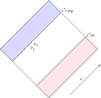
Figure 2: The points $p_{n}$, the TIF $\{x^{\mu}:x^{+}\geq\pi/\mu\}$ and the TIP $\{x^{\mu}:x^{+}\leq 0\}$ in the $x^{\pm}$ plane.

A sequence of points $p_{n}$ with $x^{+}(p_{n})=\pi/\mu$ and $x^{-}(p_{n})\rightarrow-\infty$ define PIFs $P_{n}^{*}=I^{+}(p_{n})$ which approach the TIF $T^{*}=\{x^{\mu}:x^{+}\geq\pi/\mu\}$. Using the result of the previous paragraph, the PIPs $P_{n}=I^{-}(p_{n})$ defined by this sequence each contain the TIP $T=\{x^{\mu}:x^{+}\leq 0\}$. Using an appropriately time-translated version of (10), in the limit $x^{-}(p_{n})\rightarrow-\infty$, the past of $p_{n}$ contains only points with $x^{+}\leq 0$. Thus, the $P_{n}$ approach $T$. Hence, we should identify $T$ and $T^{*}$. By time-translation, every TIF $\{x^{\mu}:x^{+}\geq x^{+}_{1}+\pi/\mu\}$ is identified with the TIP $\{x^{\mu}:x^{+}\leq x^{+}_{1}\}$. This completes the demonstration of the identification between TIPs and TIFs. Again we see that it is possible to pass beyond infinity and return to the original spacetime.

We can also use this to show that the line of TIPs is a null line in $\hat{M}$. There is a natural causal relationship between the IPs in $\hat{M}$, under which $P$ is to the causal past of $Q$ in $\hat{M}$ if $P\subset Q$. Under this causal relationship, the TIPs form a causal line; the TIP $P$ defined by $x^{+}\leq x^{+}_{P}$ is clearly to the past of the TIP $Q$ defined by $x^{+}\leq x^{+}_{Q}$ iff $x^{+}_{P}\leq x^{+}_{Q}$. Now two causally-separated points $P$ and $Q$ are null separated if there is a sequence of points $P_{n}$ which approaches $P$ but none of the points $P_{n}$ is causally separated from $Q$. Consider $x^{+}_{Q}=x^{+}_{P}+\epsilon$ for some small $\epsilon$. We have just demonstrated that the sequence of PIPs $I^{-}(p_{n})$ where $x^{+}(p_{n})=x^{+}_{P}+\pi/\mu$ approaches $P$, but $I^{-}(p_{n})$ contains points with $x^{+}=x^{+}_{P}+\pi/\mu-\delta$, which are not in $Q$. Hence the $P_{n}$ are not causally related to $Q$, and $P$ and $Q$ must be null separated.

As advertised, we have reconstructed the result that the set of ideal points is the null line $\cal I$ parametrised by $x^{+}$ together with the two points $i^{\pm}$. We will see below that this construction generalises readily to many other cases.

3 Homogeneous plane waves

For homogeneous plane waves, where the coefficient functions $\mu^{2}_{ij}$ in (1) are constants, the non-trivial components of the Weyl tensor are

$$C_{+i+j}=\mu^{2}_{ij}-{1\over n}\mu^{2}_{kk}\delta_{ij},$$ (11)

$i,j,k=1,\ldots,n$. Thus, the metric is conformally flat iff $\mu^{2}_{ij}=\mu^{2}\delta_{ij}$, that is, it is conformally flat only for the maximally symmetric case considered above (and a case with $\mu^{2}$ negative discussed below). There are many examples of particular interest to string theory which do not fall into this category; and for which it is therefore quite complicated to find an explicit Penrose-style conformal compactification. For instance, the maximally supersymmetric 11d plane wave [14], the Penrose limit of $AdS_{3}\times S^{3}\times M_{4}$ [24], and Penrose limits of less supersymmetric ten-dimensional geometries, such as the Pilch-Warner solution [19, 20, 21], are not conformally flat. (Other examples where different homogeneous plane waves arise as Penrose limits are discussed in [25, 26, 27]). Nevertheless, one can readily study the infinity of these spacetimes using the methods [23] just described. In this section, we will find the TIPs and TIFs for all homogeneous plane waves.

For almost all cases, the set of ideal points is identical to that found in the previous section, namely a single null line. This suggests that these more general examples might also have quantum-mechanical dual descriptions. This is the more surprising as the discussion includes cases where some of the eigenvalues of $\mu^{2}_{ij}$ are negative. The presence of such negative eigenvalues is believed to lead to an instability in the string sigma-model, as was discussed in [20]. Nevertheless, from the point of view of the asymptotic structure of spacetime, these examples behave in the same way as cases with all eigenvalues positive.

We consider a spacetime of the form (1). For arbitrary $\mu^{2}_{ij}$, we can make a rotation on the $x^{i}$ to make $\mu^{2}_{ij}$ diagonal. We assume there is at least one positive eigenvalue, and write the metric as

$$ds^{2}=-2dx^{+}dx^{-}-(\mu_{1}^{2}x_{1}^{2}+\ldots+\mu_{j}^{2}x_{j}^{2}-m_{1}^{2}y_{1}^{2}-\ldots-m_{n-j}^{2}y_{n-j}^{2})(dx^{+})^{2}+dx^{i}dx^{i}+dy^{a}dy^{a},$$ (12)

where $\mu_{1}\geq\mu_{2}\geq\ldots\geq\mu_{j}$. As in the previous discussion, the first step is to determine the TIPs and TIFs. As before, a future-directed timelike curve $\gamma$ must move in the direction of increasing $x^{+}$, so it will either extend to arbitrary values of $x^{+}$ or approach some constant value of $x^{+}$. Again, it will become clear below that a causal curve reaching arbitrarily large values of $x^{+}$ has the entire spacetime as its TIP. All other causal curves asymptote in the future to a constant value of $x^{+}$. Curves that asymptote to distinct values of $x^{+}$ have distinct TIPs, while we again claim that all curves asymptoting to the same value of $x^{+}$ have the same TIP. If $\mu^{2}_{ij}$ has all positive eigenvalues, the proof of this statement is as before: the curve will reach divergent $x^{-}$, and the past of any point is at least its past in the Minkowski metric. If some of the eigenvalues are negative, the statement is still true, but the proof is slightly more complicated than in the positive definite case and has been placed in appendix A. In particular, this appendix shows that the TIP of any causal curve asymptoting to $x^{+}=x^{+}_{1}$ consists exactly of those points with values of $x^{+}$ smaller than the $x_{1}^{+}$. Thus, the TIPs form a one dimensional line parametrised by $x^{+}$, together with the single point $i^{+}$ (which one may regard as the continuation of the line to $x^{+}=+\infty$). Similarly, the TIFs form a line parametrised by $x^{+}$, together with $i^{-}$ (at $x^{+}=-\infty$).

Finally, we need to determine the relation between TIPs and TIFs. The following curves are causal so long as $C(x^{+})$ is an increasing function and $A^{i},B^{i}$ are constants:

$$x^{i} = A^{i}\sin(\mu_{i}x^{+}),$$ (13)

$$y^{a} = B^{a}\sinh(m_{a}x^{+}),$$ (14)

$$x^{-} = \frac{1}{2}(x^{i}\partial_{+}x^{i}+y^{i}\partial_{+}y^{i})+C(x^{+})$$ (15)

$$= \frac{1}{2}\frac{(A^{i})2}{2}\mu_{i}\sin(\mu_{i}x^{+})\cos(\mu_{i}x^{+})+\frac{(B^{a})^{2}}{2}m_{a}\sinh(m_{a}x^{+})\cosh(m_{a}x^{+})+C(x^{+})$$ (16)

$$= \frac{\mu_{1}x_{1}^{2}}{2}\cot(\mu_{1}x^{+})+\ldots$$ (17)

Thus, the future of the origin ($x=0,y=0,x^{+}=0,x^{-}=0$) is exactly the set with

$$2x^{-}\geq\mu_{1}x_{1}^{2}\cot(\mu_{1}x^{+})+\ldots$$ (18)

until our family of null curves encounters the first caustic at $x^{+}=\pi/\mu_{1}$.

Now, take $x^{+}=\pi/\mu_{1}-\epsilon.$ By taking $\epsilon$ sufficiently small, we can arrange for (18) to be satisfied for any $x_{1}\neq 0$ (since, from the convention that $\mu_{1}$ is the largest eigenvalue, the terms not written explicitly will remain finite as $\epsilon\to 0$). Since the future is a closed set, we see that the origin is in the past of every point on the $x^{+}=\pi/\mu_{1}$ plane. By translation invariance, the past of any point with $x^{+}=x^{+}_{1}$ contains all points with $x^{+}\leq x^{+}_{1}-\pi/\mu_{1}$. In particular, it is now clear that the TIP of any curve reaching arbitrarily large values of $x^{+}$ is the entire spacetime. The remaining step of identifying future boundary points with past boundary points now follows just as in section 2 by arguing that the sequence of points $p_{n}$ such that $x^{+}=x^{+}_{1}$ and $x^{-}\to-\infty$ has PIFs $I^{+}(p_{n})$ approaching the TIF $\{x^{\mu}:x^{+}\geq x^{+}_{1}\}$ and by (18) has PIPs $I^{-}(p_{n})$ approaching the TIP $\{x^{\mu}:x^{+}\leq x^{+}_{1}-\pi/\mu_{1}\}$. Thus, this TIP and TIF are identified for each $x_{1}^{+}$. We can show as before that this is a null line.

To summarise, we have shown that for constant $\mu^{2}$ with at least one positive eigenvalue, the set of ideal points is a single null line parametrised by $x^{+}$, together with the two points $i^{\pm}$.

3.1 No positive eigenvalues

For completeness, we now mention the case of the plane wave with no positive eigenvalues. Leaving aside flat space ($\mu^{2}_{ij}=0$), these cases with negative eigenvalues are unphysical, as no such solution can arise in string theory (so long as we keep the symmetry associated with the Killing vector $\partial_{+}$, so the dilaton is constant). The point is that the non-vanishing Ricci tensor component, $R_{++}$, is essentially just the sum of the eigenvalues. However, negative $R_{++}$ in the Einstein frame violates the weak null energy condition. Hence, these backgrounds are not solutions to any known string theory.

Nevertheless, we will consider this case briefly, because it results in a different structure than the cases with positive eigenvalues. For simplicity, we will consider the special case where the metric is conformally flat, and take $\mu^{2}_{ij}=-\delta_{ij}$. The metric is then

$$ds^{2}=-2dx^{+}dx^{-}+y^{2}(dx^{+})^{2}+dy^{2}.$$ (19)

We can use the conformal boundary technique; simply apply the change of variables

$$v = x^{-}-(y^{2}/2)\tanh x^{+}$$ (20)

$$u = \tanh x^{+}$$ (21)

$$\tilde{y} = y/\cosh x^{+},$$ (22)

to obtain the metric

$$ds^{2}=(1-u^{2})^{-1}\left(-2dudv+d\tilde{y}^{2}\right),$$ (23)

with $-1<u<1.$ This shows explicitly that the spacetime (19) is conformally equivalent to a slice of Minkowski space bounded by two null planes.

As a result, the conformal boundary of (19) consists of null planes at $u=\pm 1$ and two null lines which represent the intersection of the region $-1<u<1$ with the past and future infinity of the Minkowski space described by the conformally rescaled metric $d\tilde{s}^{2}=-2dudv+d\tilde{y}^{2}.$ We see that this is qualitatively different from the other homogeneous plane waves.

4 General plane waves

We will now discuss the cases where $\mu^{2}_{ij}$ are functions of $x^{+}$. A particularly interesting example of this type is provided by the Penrose limits of near D$p$-brane spacetimes obtained in [20]. Since the near D$p$-brane geometries for $p\leq 4$ all have dual field theory descriptions [22], these cases may also lead to interesting insights into gauge/gravity connections. The resulting plane waves can have eigenvalues which become negative for some range of $x^{+}$.

When $\mu^{2}_{ij}$ is a function of $x^{+}$, there may be limitations on the range of $x^{+}$ (if the functions diverge at some finite $x^{+}$), and this can lead to interesting structures of TIPs associated with timelike curves which approach the maximum value. However, this structure will depend in a complicated way on the particular functions involved, and we are more interested in considering the effects on the one-dimensional line of ideal points parametrised by $x^{+}$ we previously considered. Therefore we will focus on the TIPs associated with causal curves which asymptotically approach some constant value of $x^{+}$ where $\mu^{2}_{ij}$ is not diverging. It is easy to extend the previous arguments to show that the TIP associated with such curves is again a region of the form $x^{+}\leq x^{+}_{1}$, so that there is a set of TIPs parametrised by $x^{+}$ (and similarly for TIFs). The details are given in the appendix. To see whether these TIPs and TIFs are identified, we need to consider specific examples, to which we now turn.

4.1 Limits of D$p$-branes

We want to consider the plane waves obtained from Penrose limits of near D$p$-branes for $p\leq 4$, as in [20]. Null geodesics in the near D$p$-brane spacetimes emerge from the brane singularity at a finite affine parameter in the past and return at a finite affine parameter in the future. As a result, the associated plane waves are singular with the eigenvalues of $\mu^{2}$ diverging at finite values of $x^{+}$, say $x^{+}=\pm x^{+}_{0}$. The divergence is of the form $\mu^{2}\rightarrow+\infty$ for $p=4$ and $\mu^{2}\rightarrow-\infty$ for $p=0,1,2.$

Due to the singularities at $x^{+}=\pm x^{+}_{0}$, it is clear that infinity is formed only from the TIPs and TIFs of causal curves that asymptote to null planes with $|x^{+}|<x^{+}_{0}$. As a result, the boundary will consist of the singular null planes together with a null line (or perhaps two) at infinity. It remains only to determine any identifications between past and future infinity.

Let us begin with the case $p=4$. Here, we see from equation (5.42) of [20] that the eigenvalues are always positive and diverge as $(x^{+}-x^{+}_{0})^{-2}$ at the singularities. Thus, the frequency of the harmonic oscillator diverges as $(x^{+}-x^{+}_{0})^{-1}$ and the oscillator oscillates infinitely many times before reaching the singularity. From our earlier discussion of the behaviour of light cones, it follows that each point on future infinity is thus identified with some point on past infinity, and vice versa. This is true even for the points close to the singularities.

Turning now to the cases $p=0,1,2,$ recall that the basic feature associated with identifications between past and future infinity is the existence of two values $x^{+}_{1},x^{+}_{2}$ of $x^{+}$ such that the future of any point on the plane $x^{+}=x^{+}_{1}$ contains every point on the plane with $x^{+}=x^{+}_{2}$. In particular, it contains points $(x^{-},x^{i},x^{+}=x^{+}_{2})$ with arbitrarily large and negative values of $x^{-}$. In section 3, such behaviour was the a result of a harmonic oscillator oscillating though half of a period.

Our strategy here is much the same as in the constant $\mu^{2}$ cases, though the treatment is necessarily less explicit. The reader may verify that the null cone of a point is again traced out by null geodesics satisfying

$$\partial_{+}^{2}x^{i} = -\mu^{2}_{ij}x^{j},$$ (24)

$$x^{-} = \frac{1}{2}x^{i}\partial_{+}x^{i}+C,$$ (25)

where $C$ is a constant. Points on past and future infinity will be identified only if there is some sequence of points on this null cone for which $x^{-}$ diverges while $x^{i}$ remains finite. It is clear that this in turn can happen only if the dimensionless ratio $x^{i}\partial_{+}x^{i}/x^{2}$ diverges toward negative infinity. Consulting [20], we see that for any $x^{+}$ the coordinate called $\phi$ in that reference is always associated with the largest eigenvalue of $\mu^{2}$, and thus the shortest period. As a result, it is sufficient to consider only this direction and to set the other coordinates to zero.

Because of the complicated dependence on $x^{+}$, the above expressions are difficult to analyse analytically. However, it is straightforward to solve the equations numerically with various initial data $\phi(0),\partial_{+}\phi(0)$. Of course, only the ratio $\frac{\partial_{+}\phi(0)}{\phi(0)}$ can effect the scale invariant quantity $x^{i}\partial_{+}x^{i}/x^{2}=\partial_{+}\phi/\phi$. If identifications occur, the ratio $x^{i}\partial_{+}x^{i}/x^{2}=\partial_{+}\phi/\phi$ evolves from positive infinity when the light cone is emitted to negative infinity when the identification occurs. In particular this ratio, and thus $\partial_{+}\phi$, goes through zero in between. If we wish to find identifications, it is to our advantage to choose a light cone which spends as much time as possible near $x^{+}=0$ where the harmonic oscillator frequencies are highest. As a result, it is best to choose the zero of $\partial_{+}\phi$ to occur at $x^{+}=0$.

Thus, one need only consider the initial data $\phi(0)=1,\partial_{+}\phi(0)=0.$ In each case ($p=0,1,2$), one finds that the ratio $\partial_{+}\phi/\phi$ is in fact bounded below. More specifically, at $x^{+}=0$ we have $\phi=1$, after which $\phi$ decreases to a positive minimum and then turns around and begins to increase. The coordinate $\phi$ is still increasing when the singularity is encountered. We therefore conclude that there are no identifications between past and future infinity in these spacetimes.

5 Discussion

We have discussed the asymptotic structure of plane waves using the approach to constructing ideal points based on past-sets as introduced in [23]. We first reconsidered the asymptotic structure of the maximally-supersymmetric ten-dimensional plane wave from this point of view. We showed that we can reproduce the results of [12], who constructed the Penrose diagram for this case. We believe the current approach offers some useful additional insight into the relation between bulk and boundary in this case; in particular, it emphasises the importance of the identifications between past and future boundaries, which are quite non-trivial in the original coordinate system. As is apparent form the conformal embedding of the BFHP wave into the Einstein static universe, these ideal points can also be reached by spacelike curves. While we have not addressed this explicitly, it is clear from our analysis that any spacelike curve which asymptotes to $x^{+}=x^{+}_{0}$ with sufficiently rapidly diverging $x^{-}$ reaches the same ideal point as do causal curves with the same asymptotics.

The real power of the approach of [23], however, is that it can easily be extended to more general metrics. We have shown that the general homogeneous plane wave has an identical causal boundary, with a one-dimensional line of ideal points, so long as there is at least one positive eigenvalue of $\mu^{2}_{ij}$. Surprisingly, the asymptotic structure is unchanged when we introduce negative eigenvalues, even though these will produce dramatic changes in the dynamical behaviour of both particles and strings in the spacetime. So long as there is at least one positive eigenvalue, there remains the possibility to pass beyond infinity and return to the original spacetime.

The most interesting direction for future work is to explore the consequences for possible holographic dual descriptions of these spacetimes. As in the previously-studied maximally supersymmetric case [12], the structure of the asymptotic boundary, and in particular the fact that it is both to the future and the past of regions of spacetime, can be viewed as evidence in favour of the existence of a quantum-mechanical dual description. For cases where a dual field theory description is expected to exist, such as the maximally supersymmetric 11d plane wave which arises in the Penrose limit of $AdS_{4}\times S^{7}$, this result is satisfying but perhaps unsurprising. However, we find that the relevant behaviour is far more general than this. It would be especially interesting if further evidence could be found for the existence of a holographic dual for the cases with some negative eigenvalues.

In the more general case where $\mu^{2}_{ij}$ are functions of $x^{+}$, the analysis is more complicated, but in many cases at least some of this structure will survive. We have explored in detail the asymptotic structure of the cases arising from Penrose limits of D$p$-branes, finding that there is a set of TIPs and TIFs which form a one-dimensional line segment parametrised by $x^{+}$; the TIPs and TIFs are identified for $p=4$ but not for $p=0,1,2$. It would be interesting to extend this further to investigate more time-dependent examples.

Figure 3: The asymptotic structure of a plane wave that has $\mu^{2}_{ij}=0$ before $x^{+}=x^{+}_{0}.$ The null plane $x^{+}=x^{+}_{0}$ intersects past infinity only at the marked point. Heavy line segments indicate potential identifications between past and future infinity.

One interesting case occurs when the matrix $\mu_{ij}^{2}$ remains diagonal but vanishes in, say, the asymptotic past. Suppose in particular that no harmonic oscillator oscillates more than some finite number of times in the past. In this case past infinity is essentially that of flat Minkowski space! The details become clear if we suppose that $\mu_{ij}^{2}$ is strictly zero before some $x^{+}=x^{+}_{0}$. The region to the past of $x^{+}_{0}$ is the part of Minkowski space below some null plane $P$, whose past boundary is that of Minkowski space except for a half line to the future of the point on past infinity where $x^{+}=x^{+}_{0}$ (see figure 3). Thus, whether and how this half line is identified with part of future infinity is determined by the behaviour of the harmonic oscillators to the future of $x^{+}_{0}$.

Another avenue for future development is to explore the asymptotic structure for pp-waves, where a more general dependence on $x^{i}$ is allowed. These are also exact backgrounds for string theory, at least to all orders of perturbations in $\alpha^{\prime}$. Specific examples have recently been considered in [28], where string propagation on such backgrounds was considered, and connections to two-dimensional integrable systems were noted. Finally, we plan to address detailed issues of the identifications that were suppressed here in a forthcoming paper.

Appendix A Appendix: TIPs of the general plane wave

In this appendix we show that the TIP of any causal curve asymptoting in the future to $x^{+}=x^{+}_{1}$ is given by $\{x^{\mu}:x^{+}\leq x^{+}_{1}\}$. In particular, all causal curves which asymptote to the same value of $x^{+}$ have the same TIP. We will consider the general metric (1), assuming only that the functions $\mu^{2}_{ij}(x^{+})$ are regular in an open neighbourhood of $x^{+}=x^{+}_{1}$.

The non-trivial step in showing that the TIP is the region $\{x^{\mu}:x^{+}\leq x^{+}_{1}\}$ is to show that the past of the curve includes all points on the surface $x^{+}=x^{+}_{1}-\delta$ for arbitrarily small $\delta$. The past of this null surface will clearly include all points with smaller $x^{+}$, so if we can show this, it will follow that the TIP contains the open set $\{x^{\mu}:x^{+}<x^{+}_{1}\}$. We also know that the TIP cannot contain any points with $x^{+}>x^{+}_{1}$, since no causal curve can move in the direction of decreasing $x^{+}$. Hence, since the TIP is a closed set, it will be precisely $\{x^{\mu}:x^{+}\leq x^{+}_{1}\}$.

We therefore need only consider the behaviour in a small neighbourhood of the surface $x^{+}=x^{+}_{1}$, so we may approximate the functions $\mu^{2}_{ij}(x^{+})$ by constants $\mu^{2}_{ij}(x^{+}_{1})$ and diagonalise this matrix in the neighbourhood of $x^{+}=x^{+}_{1}$ by a rotation on the $x^{i}$. The result is a metric of the form (12). We will also redefine the $x^{+}$ coordinate so that the surface to which the curve asymptotes is at $x^{+}=0$.

Let us now study the causal future of the origin of coordinates in the metric (12). Consider the new set of null curves given by

$$x^{i}=A_{i}\sinh(\mu_{i}x^{+}),\ \ y^{a}=B_{a}\sin(m_{a}x^{+}),\ \ x^{-}=(1/2)(\mu_{i}^{2}A_{i}^{2}+m_{a}^{2}B_{a}^{2})x^{+}.$$ (26)

(Note that these are different from the causal curves considered earlier; in particular, $\sin$ and $\sinh$ are interchanged.) These show us that all points satisfying

$$x^{-}\geq\frac{1}{2}x^{+}\left(\sum_{i}\left(\frac{\mu_{j}x^{j}}{\sinh(\mu_{j}x^{+})}\right)^{2}+\sum_{b}\left(\frac{m_{b}y_{b}}{\sin(m_{b}x^{+})}\right)^{2}\right)$$ (27)

are in the causal future of the origin. But for $x^{+}<\delta_{1}$ and small enough $\delta_{1}$, the Taylor expansions yield

$$x^{-} \geq \frac{x^{2}+y^{2}}{2x^{+}(1-\epsilon_{1})},\ \ \ {\rm or}$$ (28)

$$y^{2}+x^{2} \leq 2(1-\epsilon_{1})x^{-}x^{+}$$ (29)

for any $\epsilon_{1}$. More generally, for $\Delta x^{+}<\delta_{1}$ and small enough $\delta_{1}$, the future of the point $x^{i}=0,y^{i}=0,x^{-}=0,x^{+}=x^{+}_{0}$ contains all points satisfying

$$x^{2}+y^{2}\leq 2(1-\epsilon_{1})x^{-}\Delta x^{+}.$$ (30)

Let us call this region $R_{x^{+}_{0}}$.

Now consider any causal curve that asymptotes in the future to the surface $x^{+}=0$. We want to show that this enters the future of the point $x^{i}=0,y^{i}=0,x^{-}=0,x^{+}=x^{+}_{0}<0$ for small enough $|x^{+}_{0}|$. Explicitly, this future region $R_{x^{+}_{0}}$ is

$$y^{2}+x^{2}\leq 2(1-\epsilon_{1})x^{-}|x^{+}_{0}|.$$ (31)

Since any point can be brought to $x^{i}=0,y^{a}=0,x^{-}=0,x^{+}=x^{+}_{0}$ by a symmetry transformation that does not act on $x^{+}$, we will have shown that any causal curve which asymptotes to $x^{+}=0$ enters the future of any point having $x^{+}<0$.

Consider then an arbitrary causal curve that asymptotes to $x^{+}=0$. Below, we use dots to denote $d/dx^{+}$. Causality implies

$$2\dot{x}^{-}\geq(m_{a}^{2}y_{a}^{2}-\mu_{i}^{2}x_{i}^{2})+\dot{y_{a}}^{2}+\dot{x_{i}}^{2}\geq(-\mu_{i}^{2}x_{i}^{2})+\dot{y_{a}}^{2}+\dot{x_{i}}^{2}.$$ (32)

Now, some coordinate (and therefore some velocity) must diverge at $x^{+}=0$. If only $x^{-}$ diverges while $x_{i},y_{a}$ remain bounded, then it is clear that the curve enters $R_{x^{+}_{0}}$. If $x_{i}$ do not diverge, then some $y_{a}$ and $\dot{y_{a}}$ diverge, and close enough to $x^{+}=0$ we achieve

$$2\dot{x}^{-}\geq(1-\epsilon_{2})(\dot{x_{i}}^{2}+\dot{y_{a}}^{2}).$$ (33)

But if some $x_{i}$ diverge, then $\ln x_{i}$ and $\partial_{+}\ln x_{i}$ diverge, so that we have $\dot{x}_{i}\gg x_{i}$ and again we achieve $2\dot{x}^{-}\geq(1-\epsilon_{2})(\dot{x_{i}}^{2}+\dot{y_{a}}^{2}).$ We will use this relation below, and also the corollary that $x^{-}$ must diverge at $x^{+}=0$.

For the final step, let us introduce a new (fiducial and completely non-physical) metric

$$ds^{2}_{\rm fid}=-2dx^{+}dx^{-}+(1-\epsilon_{2})(dx^{2}+dy^{2}),$$ (34)

and note that sufficiently close to $x^{+}=0$ our curve is also causal with respect to this fiducial metric. So, if we choose any point $x^{i}_{1},y^{a}_{1},x^{-}_{1},x^{+}=-\epsilon_{3}$ close to $x^{+}=0$ on our causal curve, the curve remains in the fiducial future light cone of this point. That is, the curve satisfies

$$y^{2}+x^{2}\leq\frac{2}{1-\epsilon_{2}}(x^{-}-x^{-}_{1})\epsilon_{3}.$$ (35)

This controls the rate at which $x_{i}$ and $y_{a}$ can diverge with $x^{-}$. For $2\epsilon_{3}\leq(1-\epsilon_{2})(1-\epsilon_{1})|x^{+}_{0}|$, we see that our causal curve cannot run to large $x^{-}$ without entering the region

$$y^{2}+x^{2}\leq 2(1-\epsilon_{1})x^{-}|x^{+}_{0}|,$$ (36)

and thus the future of $x_{i}=0,y_{a}=0,x^{-}=0,x^{+}=x^{+}_{0}$. Hence any casual curve $\gamma$ asymptoting to $x^{+}=0$ has this point, and thus any point with $x^{+}<0$, in its causal past. This completes the proof that the TIP $I^{-}[\gamma]$ is $\{x^{\mu}:x^{+}\leq 0\}$.

- [1] M. W. Brinkmann, “On Riemann spaces conformal to Euclidean spaces,” Proc. Natl. Acad. Sci. U.S., 9 (1923) 1, see section 21.5.
- [2] H. Bondi, F.A.E. Pirani, and I. Robinson, “Gravitational waves in general relativity III: Exact plane waves,” Proc. Roy. Soc. Lond. A 251 (1959) 519.
- [3] J. Hély, Compt. rend. 249 (1959) 1867.
- [4] A. Peres, “Some Gravitational Waves,” Phys. Rev. Lett. 3, 571 (1959) [arXiv:hep-th/0205040].
- [5] J. Ehlers and W. Kundt, “Exact Solutions of the gravitational field equations” in Gravitation: An introduction to current research, ed. by L. Witten (Wiley, New York, 1962).
- [6] D. Kramer, H. Stephani, E. Herlt, M. MacCallum, and E. Schmutzer, Exact Solutions of Einstein’s field equations (Cambridge, 1979).
- [7] D. Amati and C. Klimcik, “Nonperturbative computation of the Weyl anomaly for a class of nontrivial backgrounds,” Phys. Lett. B 219 (1989) 443; G. T. Horowitz and A. R. Steif, “Space-Time Singularities In String Theory,” Phys. Rev. Lett. 64 (1990) 260.
- [8] R. R. Metsaev, “Type IIB Green-Schwarz superstring in plane wave Ramond-Ramond background,” Nucl. Phys. B 625, 70 (2002) [arXiv:hep-th/0112044].
- [9] R. Penrose, “Any geometry has a plane-wave limit”, in Differential Geometry and Relativity, ed. by Cahen and Flato (D. Reidel Publishing, Dordrecht-Holland, 1976).
- [10] D. Berenstein, J. M. Maldacena and H. Nastase, “Strings in flat space and pp waves from N = 4 super Yang Mills,” JHEP 0204, 013 (2002) [arXiv:hep-th/0202021].
- [11] M. Blau, J. Figueroa-O’Farrill, C. Hull and G. Papadopoulos, “A new maximally supersymmetric background of IIB superstring theory,” JHEP 0201 (2002) 047 [arXiv:hep-th/0110242].
- [12] D. Berenstein and H. Nastase, “On lightcone string field theory from super Yang-Mills and holography,” arXiv:hep-th/0205048.
- [13] E. Kiritsis and B. Pioline, “Strings in homogeneous gravitational waves and null holography,” arXiv:hep-th/0204004.
- [14] J. Kowalski-Glikman, “Vacuum States In Supersymmetric Kaluza-Klein Theory,” Phys. Lett. B 134 (1984) 194; J. Figueroa-O’Farrill and G. Papadopoulos, “Homogeneous fluxes, branes and a maximally supersymmetric solution of M-theory,” JHEP 0108 (2001) 036 [arXiv:hep-th/0105308].
- [15] M. Blau, J. Figueroa-O’Farrill, C. Hull and G. Papadopoulos, “Penrose limits and maximal supersymmetry,” Class. Quant. Grav. 19 (2002) L87 [arXiv:hep-th/0201081].
- [16] M. Cvetic, H. Lu and C. N. Pope, “Penrose limits, pp-waves and deformed M2-branes,” arXiv:hep-th/0203082; M. Cvetic, H. Lu and C. N. Pope, “M-theory pp-waves, Penrose limits and supernumerary supersymmetries,” arXiv:hep-th/0203229.
- [17] I. Bena and R. Roiban, “Supergravity pp-wave solutions with 28 and 24 supercharges,” arXiv:hep-th/0206195.
- [18] J. Michelson, “A pp-wave with 26 supercharges,” arXiv:hep-th/0206204.
- [19] R. Corrado, N. Halmagyi, K. D. Kennaway and N. P. Warner, “Penrose limits of RG fixed points and pp-waves with background fluxes,” arXiv:hep-th/0205314.
- [20] E. G. Gimon, L. A. Pando Zayas and J. Sonnenschein, “Penrose limits and RG flows,” arXiv:hep-th/0206033.
- [21] D. Brecher, C. V. Johnson, K. J. Lovis and R. C. Myers, “Penrose limits, deformed pp-waves and the string duals of N = 1 large N gauge theory,” arXiv:hep-th/0206045.
- [22] N. Itzhaki, J. M. Maldacena, J. Sonnenschein and S. Yankielowicz, “Supergravity and the large N limit of theories with sixteen supercharges,” Phys. Rev. D 58 (1998) 046004 [arXiv:hep-th/9802042].
- [23] R. Geroch, E. H. Kronheimer, and R. Penrose, “Ideal points in space-time”, Proc. Roy. Soc. Lond. A 327 (1972) 545.
- [24] M. Blau, J. Figueroa-O’Farrill and G. Papadopoulos, “Penrose limits, supergravity and brane dynamics,” arXiv:hep-th/0202111.
- [25] V. E. Hubeny, M. Rangamani and E. Verlinde, “Penrose limits and non-local theories,” arXiv:hep-th/0205258.
- [26] Y. Oz and T. Sakai, “Penrose limit and six-dimensional gauge theories,” arXiv:hep-th/0207223.
- [27] M. Alishahiha and A. Kumar, “PP-waves from nonlocal theories,” arXiv:hep-th/0207257.
- [28] J. Maldacena and L. Maoz, “Strings on pp-waves and massive two dimensional field theories,” arXiv:hep-th/0207284.