Loop Quantum Gravity and Ultra High Energy Cosmic Rays

Abstract

There are two main sets of data for the observed spectrum of ultra high energy cosmic rays (those cosmic rays with energies greater than $\sim 4\times 10^{18}$ eV), the High Resolution Fly’s Eye (HiRes) collaboration group observations, which seem to be consistent with the predicted theoretical spectrum (and therefore with the theoretical limit known as the Greisen-Zatsepin-Kuzmin cutoff), and the observations from the Akeno Giant Air Shower Array (AGASA) collaboration group, which reveal an abundant flux of incoming particles with energies above $1\times 10^{20}$ eV violating the Greisen-Zatsepin-Kuzmin cutoff. As an explanation of this anomaly it has been suggested that quantum-gravitational effects may be playing a decisive role in the propagation of ultra high energy cosmic rays. In this article we take the loop quantum gravity approach. We shall provide some techniques to establish and analyze new constraints on the loop quantum gravity parameters arising from both sets of data, HiRes and AGASA . We shall also study their effects on the predicted spectrum for ultra high energy cosmic rays. As a result we will state the possibility of reconciling the AGASA observations.

I Introduction

In this article we are concerned with the observation of ultra high energy cosmic rays (UHECR), i.e. those cosmic rays with energies greater than $\sim 4\times 10^{18}$ eV. Although not completely clear, it has been suggested that these high energy particles are possibly heavy nuclei exp1 ; Ave (we will assume here that they are protons) and, by virtue of the isotropic distribution with which they arrive to us, that they originate in extragalactic sources.

A detailed understanding of the origin and nature of UHECR is far from being achieved; the way in which the observed cosmic ray spectrum appears to us still is a mystery and a matter of great debate. A first subject of interest (faced with the lack of reasonable mechanisms) is how such energetic particles have been accelerated to energies well above $4\times 10^{18}$ eV by its sources. A second subject of interest is the study of their propagation in open space through the cosmic microwave background radiation (CMBR), whose presence necessarily produce a friction on UHECR making them release energy in the form of secondary particles and affecting their possibility to reach great distances. A first estimation of the characteristic distance that UHECR can reach before losing most of their energy was simultaneously made in 1966 by K. Greisen Greisen and G. T. Zatsepin & V. A. Kuzmin Zatsepin & Kuzmin , who showed that the observation of cosmic rays with energies greater than $4\times 10^{19}$ eV should be greatly suppressed. This energy ($4\times 10^{19}$ eV) is usually referred as to the GZK cutoff energy. Similarly and a few years later, F.W. Stecker Stecker calculated the mean life time for protons as a function of their energy, giving a more accurate perspective of the energy behavior of the cutoff and showing that cosmic rays with energies above $1\times 10^{20}$ eV should not travel more than $\sim 100$ Mpc. More detailed approaches to the GZK-cutoff feature have been made since these first estimations. For example V. Berezinsky & S.I. Grigorieva Berezinsky2 , V. Berezinsky et al. Berezinsky and S.T. Scully & F.W. Stecker Scully & Stecker have made progress in the theoretical study of the spectrum $J(E)$ (i.e. the flux of arriving particles as a function of the observed energy $E$) that UHECR should present. As a result, the GZK cutoff exists in the form of a suppression in the predicted flux of cosmic rays with energies above $\sim 8\times 10^{19}$ eV.

At present there are two main different sets of data for the observed flux $J(E)$ in its most energetic sector ($E>4\times 10^{18}$ eV). On one hand we have the observations from the High Resolution Fly’s Eye (HiRes) collaboration group HiRes , which seem to be consistent with the predicted theoretical spectrum and, therefore, with the presence of the GZK cutoff. Meanwhile, on the other hand, we have the observations from the Akeno Giant Air Shower Array (AGASA) collaboration group exp3 , which reveal an abundant flux of incoming cosmic rays with energies above $1\times 10^{20}$ eV. The appearance of these high energy events is greatly opposed to the predicted GZK cutoff, and a great challenge that has motivated a vast amount of new ideas and mechanisms to explain this phenomenon Tkachev 1 ; Tkachev 2 ; Tkachev 4 ; Monopoles ; Z-Burst1 ; Z-Burst2 ; Z-Burst3 ; Super-relic . If the AGASA observations are correct then, since there are no known active objects in our neighborhood (let us say within a radius $R\simeq 100$ Mpc) able to act as sources of such energetic particles and since their arrival is mostly isotropic (without any privileged local source), we are forced to conclude that these cosmic rays come from distances larger than $100$ Mpc. This is commonly referred as the Greisen-Zatsepin-Kuzmin (GZK) anomaly.

One of the interesting notions emerging from the possible existence of the GZK anomaly is that, since ultra high energy cosmic rays involve the highest energy events registered up to now, then a possible framework to understand and explain this phenomena could be of a quantum-gravitational nature KIFUNE ; Amelino-Piran1 ; Ellis ; Amelino-Piran2 ; Amelino ; Alfaro & Palma . This possibility is indeed very exciting if we consider the present lack of empirical support for the different approaches to the problem of gravity quantization. In the context of the UHECR phenomena, all these different approaches motivated by different quantum gravity formulations, have usually converged on a common path to solve and explain the GZK anomaly: the introduction of effective models for the description of high energy particle propagation. These effective models, pictures of the yet unknown full quantum gravity theory, offer the possibility to modify conventional physics through new terms in the equations of motion (now effective equations of motion), leading to the eventual breakup of fundamental symmetries such as Lorentz invariance (expected to be preserved at the fundamental level). These Lorentz symmetry breaking mechanisms are usually referred as Lorentz invariance violations (LIV’s) if the break introduce a privileged reference frame, or Lorentz invariance deformations (LID’s), if such a reference frame is absent Amelino2 ; Magueijo+Smolin ; Kowalski-Glikman . Its appearance on theoretical as well as phenomenological grounds (such as high energy astrophysical phenomena) has been widely studied, and offers a large and rich amount of new signatures that deserve attention colladay1 ; colladay2 ; Amelino & Ellis ; bertolami1 ; bertolami2 ; Liberati1 ; Major ; Noncommutativity ; Liberati2 .

To deepen the above ideas, we have adopted the loop quantum gravity (LQG) theory LQG1 ; LQG2 , one of the proposed alternatives for the yet nonexistent theory of quantum gravity. It is possible to study LQG through effective theories that take into consideration matter-gravity couplings. In this line, in the works of J. Alfaro et al. Neutrinos ; Photons ; AMU , the effects of the loop structure of space at the Planck level are treated semiclassically through a coarse-grained approximation. An interesting feature of these methods is the explicit appearance of the Plank scale $l_{p}$ and the appearance of a new length scale $\mathcal{L}\gg l_{p}$ (called the “weave” scale), such that for distances $d\ll\mathcal{L}$ the quantum loop structure of space is manifest, while for distances $d\geqslant\mathcal{L}$ the continuous flat geometry is regained. The presence of these two scales in the effective theories has the consequence of introducing LIV’s to the dispersion relations $E=E(p)$ for particles with energy $E$ and momentum $p$. It can be shown that these LIV’s can significantly modify the kinematical conditions for a reaction to take place. For instance, as shown in detail in Coleman & Glashow , if the dispersion relation for a particle $i$ is (from here on, $\hbar=c=1$)

$$E_{i}^{2}=A_{i}^{2}p_{i}^{2}+m_{i}^{2}$$ (1)

(where $E_{i}$, $p_{i}$ and $m_{i}$ are the respective energy, momentum and mass of the $i$th particle, and $A_{i}$ is a LIV parameter that can be interpreted as the maximum velocity of the $i$th particle) then the threshold condition for a reaction to take place can be substantially modified if the difference $\delta A=A_{a}-A_{b}$ is non zero ($a$ and $b$ are two particles involved in the reaction leading to the mentioned threshold) Coleman & Glashow . An interesting consequence of the above situation —for the UHECR phenomenology— is that the kinematical conditions for a reaction between a primary cosmic ray and a CMBR photon can be modified, leading to new effects and predictions such as an abundant flux of cosmic rays well beyond the GZK cutoff energy (explaining in this way the AGASA observations).

The purpose of this paper is to provide some techniques to establish and analyze new constraints on the LQG parameters (or any other LIV parameters), that will confidently rise when the experimental situation is clarified in a reliably way up to a certain energy scale. In the present case, and for the practical purpose of this paper, we shall assume that such energy scale is currently $4\times 10^{19}$ eV. Also, we shall attempt to predict (under certain assumptions) a modified UHECR spectrum arising from the LQG corrections to the conventional theory, and consistent with the AGASA observations (though we shall analyze both, HiRes and AGASA sets of data, throughout this paper we will be more concerned with the possibility that the AGASA results are the correct one). To accomplish these goals, we have organized this article as follows: In section II, “Ultra high energy cosmic rays”, we shall give a brief self contained derivation of the conventional spectrum and briefly analyze it jointly with HiRes and AGASA observations. In section III, “Loop quantum gravity”, we will present a short outline of loop quantum gravity and its effective description of fermion and electromagnetic fields (relevant for the description of UHECR propagation). In section IV, “Threshold conditions”, we will analyze the effects of LQG corrections on the threshold conditions for the main reactions involved in the UHECR phenomena to take place. In section V, “Modified spectrum”, we will show how the modified kinematics can be relevant to the theoretical spectrum $J(E)$ of cosmic rays (we will present the obtained modified spectrum). Section VI, “Conclusions”, will be reserved for some final remarks.

II Ultra High Energy Cosmic Rays

In this section we will review the main steps in the derivation of the UHECR spectrum. This presentation will be useful and relevant for the description of the kinematical effects that LQG corrections can have on the predicted flux of cosmic rays. The following material is mainly contained in the works of F.W. Stecker Stecker , Berezinsky et al. Berezinsky and S.T. Scully & F.W. Stecker Scully & Stecker .

II.1 General Description

Two simple and commonly used assumptions for the development of the cosmic ray spectrum are: 1) that the sources are uniformly distributed in the Universe, and 2) that the generation flux $F(E_{g})$ of emitted cosmic rays from the sources is correctly described by a power law behavior of the form $F(E_{g})\propto E_{g}^{-\gamma_{g}}$, where $E_{g}$ is the energy of the emitted particle and $\gamma_{g}$ is the generation index.

One of the main quantities in the calculation of the UHECR spectrum is the energy loss $-E^{-1}dE/dt$. This quantity describes the rate at which a cosmic ray loses energy, and takes into consideration two chief contributions: the energy loss due to the redshift attenuation and the energy loss due to collisions with the CMBR photons. This last contribution depends, at the same time, on the cross sections $\sigma$ and the inelasticities $K$ of the interactions produced during the propagation of protons in the extragalactic medium, as well as on the CMBR spectrum. The most important reactions taking place in the description of proton’s propagation (and which produce the release of energy in the form of particles) are the pair creation

$$p+\gamma\rightarrow p+e^{-}+e^{+},$$ (2)

and the photo-pion production

$$p+\gamma\rightarrow p+\pi.$$ (3)

This last reaction happens through several channels (for example the baryonic $\Delta$ and $N$, and mesonic $\rho$ and $\omega$ resonance channels, just to mention some of them) and is the main reason for the appearance of the GZK cutoff.

II.2 Some Kinematics

To study the interaction between protons and the CMBR, it is useful to distinguish between three reference systems; the laboratory system $\mathcal{K}$ (which we identify with the Friedman Robertson Walker (FRW) co-moving reference system), the center of mass (c.m.) system $\mathcal{K}^{*}$, and the system where the proton is at rest $\mathcal{K}^{\prime}$. In terms of these systems, the photon energy will be expressed as $\omega$ in $\mathcal{K}$ and as $\epsilon$ in $\mathcal{K}^{\prime}$. The relation between both quantities is simply

$$\epsilon=\gamma\omega(1-\beta\cos\theta),$$ (4)

where $\gamma=E/m_{p}$ is the Lorentz factor relating $\mathcal{K}$ and $\mathcal{K}^{\prime}$, $E$ and $m_{p}$ are the energy and mass of the incident proton, $\beta=\sqrt{1-\gamma^{-2}}$, and $\theta$ is the angle between the momenta of the photon and the proton measured in the laboratory system $\mathcal{K}$.

To determine the total energy $E^{*}_{\mathrm{tot}}=E^{*}+\epsilon^{*}$ in the c.m. system, it is enough to use the invariant energy squared $s\equiv E_{\mathrm{tot}}^{2}-p_{\mathrm{tot}}^{2}$ (where $E_{\mathrm{tot}}=E+\omega$ and $p_{\mathrm{tot}}$ are the total energy and momentum in the laboratory system). In this way, we have

$$E^{*\,2}_{\mathrm{tot}}=s=m_{p}^{2}+2m_{p}\epsilon.$$ (5)

As a consequence, the Lorentz factor $\gamma_{c}$ which relates the $\mathcal{K}$ reference system with the $\mathcal{K}^{*}$ system, is

$$\gamma_{c}=\frac{E+\omega}{\sqrt{s}}\simeq\frac{E}{(m_{p}^{2}+2m_{p}\epsilon)^{1/2}}.$$ (6)

Let us consider the relevant case in which the reaction between the proton and the CMBR photon is of the type

$$p+\gamma\rightarrow a+b,$$ (7)

where $a$ and $b$ are two final particles of the collision. The final energies of these particles are easily determined by the conservation of energy-momentum. In the $\mathcal{K}^{*}$ system these are

$$E_{a,\,b}^{*}=\frac{1}{2\sqrt{s}}(s+m_{a,\,b}^{2}-m_{b,\,a}^{2}).$$ (8)

Transforming this quantity to the laboratory system, and averaging with respect to the angle between the directions of the final momenta, it is possible to find that the final average energy of $a$ (or $b$) in the laboratory system is

$$<E_{a,\,b}>=\frac{E}{2}\left(1+\frac{m_{a,\,b}^{2}-m_{b,\,a}^{2}}{s}\right).$$ (9)

The inelasticity $K$ of the reaction is defined as the average fractional difference $K=\Delta E/E$, where $\Delta E=E-E_{\mathrm{f}}$ is the difference between the initial energy $E$ and final energy $E_{\mathrm{f}}$ of the proton (in a single collision with the CMBR photons). For the particular case of the emission of an arbitrary particle $a$ (that is to say $p+\gamma\rightarrow p+a$), expression (9) allows us to write

$$K_{a}(s)=\frac{1}{2}\left(1+\frac{m_{a}^{2}-m_{p}^{2}}{s}\right),$$ (10)

where $K_{a}$ is the inelasticity of the described process. This is one of the main quantities involved in the study of the UHECR spectrum, in particular, when the emitted particle $a$ is a pion.

II.3 Mean Life $\tau(E)$

To derive the UHECR spectrum it is imperative to know the mean life $\tau(E)$ of the cosmic ray (or proton) with energy $E$ propagating in space, due to the attenuation of its energy by the interactions with the CMBR photons. The mean life $\tau(E)$ is defined through the relation

$$\tau(E)^{-1}=\left(-\frac{1}{E}\frac{dE}{dt}\right)_{\mathrm{col}},$$ (11)

where the label “col” refers to the fact that the energy loss is due to the collisions with the CMBR photons. To explicitly determine the form of $\tau(E)$, let us express (11) in terms of the microscopic collision-quantities:

$$\tau(E)^{-1}=\frac{\Delta E}{E}\frac{1}{\Delta t},$$ (12)

where $\Delta E$ is the difference between the initial and final energies of the proton before and after each collision, and $\Delta t$ is the characteristic time between collisions. Introducing the inelasticity through its definition $K=\Delta E/E$, and expressing the characteristic time in terms of the scattering cross section and density $\rho$ of the target photons, we can write then:

$$\tau(E)^{-1}=K\,\sigma\rho\,v_{\mathrm{rel}},$$ (13)

where $v_{\mathrm{rel}}$ is the relative velocity between the incident proton and the background. The above relation can be driven to a more accurate version if we consider that both $v_{\mathrm{rel}}$ and $\sigma$ are functions of the energy and direction of propagation of the CMBR photons relative to the incident proton. Considering these elements we are able to write

$$d\tau(E)^{-1}=K\,\sigma\,v_{\mathrm{rel}}\eta(\omega)d\omega\,d\Omega/4\pi,$$ (14)

where $\eta(\omega)d\omega$ is the CMBR density of photons with energies in the range $[\omega$, $\omega+d\omega]$, and $d\Omega/4\pi=\sin\theta\,d\theta d\phi/4\pi$ is the section of solid angle. With the above quantities, it is simple to rewrite $v_{\mathrm{rel}}$ through

$$v_{\mathrm{rel}}\,d\Omega/4\pi=\frac{\epsilon\,d\epsilon\,d\phi}{4\pi\gamma^{2}\omega^{2}},$$ (15)

with $\epsilon\in[0,2\gamma\omega]$ and $\phi\in[0,2\pi]$. Substituting equation (15) in (14) and using the fact that the CMBR density corresponds to a Planck distribution $\eta(\omega)d\omega=\omega^{2}d\omega/\pi^{2}(e^{\omega/kT}-1)$, it is finally possible to show that the mean life $\tau(E)$ can be written in the form

$$\tau(E)^{-1}=-\frac{kT}{2\pi^{2}\gamma^{2}}\!\int_{\epsilon_{\mathrm{th}}}^{\infty}\!\!\!\!d\epsilon\,\sigma(\epsilon)K(\epsilon)\epsilon\ln[1-e^{-\epsilon/2\gamma kT}].$$ (16)

II.4 Energy Loss and Spectrum

The energy loss suffered by a very energetic proton during its journey, from a distant source to our detectors, is not only produced by the collisions that it has with CMBR at a particular epoch. There will also be a decrease in its energy due to the redshift attenuation produced by the expansion of the Universe. At the same time, such expansion will affect the collision rate through the attenuation of the photon gas density, which can be understood as a cooling of the CMBR through the relation $T=(1+z)T_{0}$, where $z$ is the redshift and $T_{0}$ is the temperature of the background at the present time. To calculate the spectrum we need to consider the rate of energy loss during any epoch $z$ of the Universe.

For the present discussion, we shall assume that the Universe is well described by a matter dominated Friedman Robertson Walker (FRW) space-time, and that the ratio of density $\Omega_{0}=\rho/\rho_{c}$ (where $\rho$ is the energy density of the present Universe and $\rho_{c}$ is the critical energy density for the Universe to be flat) is such that $\Omega_{0}=1$. The above assumptions give rise to the following relation between the temporal coordinate $t$ (proper time in the co-moving system) and the redshift $z$:

$$dt=-\frac{dz}{H_{0}(1+z)^{5/2}},$$ (17)

where $H_{0}$ is the Hubble constant at present time. Since the momentum of a free particle in a FRW space behaves as $p\propto(1+z)$, we will have, with the additional consideration $p\gg m$ (where $m$ is the particle mass), that the energy loss due to redshift is

$$\left(-\frac{1}{E}\frac{dE}{dt}\right)_{\mathrm{cr}}=H_{0}(1+z)^{3/2}.$$ (18)

On the other hand, the energy loss due to collisions with the CMBR will evolve as the background temperature changes (recall $T=(1+z)T_{0}$). This evolution can be parameterized through $z$ and is given by

$$\left(-\frac{1}{E}\frac{dE}{dt}\right)_{\mathrm{col}}=(1+z)^{3}\tau([1+z]E)^{-1}.$$ (19)

The total energy loss can be expressed as the addition of the former contributions (using $z$ instead of $t$)

$$\frac{1}{E}\frac{dE}{dz}=(1+z)^{-1}+H_{0}^{-1}(1+z)^{1/2}\tau([1+z]E)^{-1}.$$ (20)

Equation (20) can be numerically integrated to give the energy $E_{g}(E,z)$ of a proton generated by the source in a $z$ epoch and that will be detected with a energy $E$ here on Earth. Let us designate this solution by the formal expression

$$E_{g}(E,z)=\lambda(E,z)E.$$ (21)

It is also possible to manipulate equation (20) to obtain an expression for the dilatation of the energy interval $dE_{g}/dE$. To accomplish this it is necessary to integrate (20) with respect to $z$ and then differentiate it with respect to $E$ to obtain an integral equation for $dE_{g}/dE$. The solution of such an equation is found to be

$$\frac{dE_{g}(z_{g})}{dE}=(1+z_{g})\qquad\qquad\qquad\qquad$$

$$\times\exp\left[\int^{z_{g}}_{0}\frac{dz}{H_{0}}(1+z)^{1/2}\frac{db(E^{\prime})}{dE^{\prime}}\right].$$ (22)

where $E^{\prime}=(1+z)\lambda(E,z)E$.

The total flux $dj(E)$ of emitted particles from a volume element $dV=R^{3}(z)r^{2}drd\Omega$, in the epoch $z$ and coordinate $r$, measured from Earth at present with energy $E$ is

$$dj(E)dE=\frac{F(E_{0},z)dE_{0}n(z)dV}{(1+z)4\pi R_{0}^{2}r^{2}},$$ (23)

where $j(E)$ is the particle flux per energy, $F(E_{0},z)dE_{0}$ the emitted particle flux within the range $(E_{0},E_{0}+dE_{0})$, and $n(z)$ the density of sources in $z$. As previously mentioned, it is convenient to study the emission flux with a power law spectrum of the type $F(E)\propto E^{-\gamma_{g}}$. It can be shown that with such assumption, the relation between the emission flux and the total luminosity $L_{p}$ of the source is $F(E)=(\gamma_{g}-2)L_{p}E^{-\gamma_{g}}$. To describe the evolution of the sources we shall also use a power law behavior. This will be done through the relation

$$L_{p}(z)n(z) = (1+z)^{(3+m)}L_{p}(0)n(0),$$ (24)

$$= (1+z)^{(3+m)}\mathcal{L}_{0},$$

in such a way that $m=0$ corresponds to the case in which sources do not evolve. If we consider that $R_{0}=(1+z)R(z)$ and $R(z)dr=dt$ for flat spaces (and $v\simeq 1$ for very energetic particles), using (17) to express all in terms of $z$ and, finally, integrating (23) from $z=0$ to some $z=z_{max}$ for which sources are not relevant for the phenomena, it is possible to obtain

$$j(E)=(\gamma_{g}-2)\frac{1}{4\pi}\frac{\mathcal{L}_{0}}{H_{0}}E^{-\gamma_{g}}\qquad\qquad$$

$$\times\int^{z_{\mathrm{max}}}_{0}\!\!\!\!\!\!dz_{g}(1+z_{g})^{m-5/2}\lambda^{-\gamma_{g}}(E,z_{g})\frac{dE_{g}(z_{g})}{dE}.$$ (25)

The above expression constitutes the spectrum of UHECR. It remains to fix (observationally) the volumetric luminosity $\mathcal{L}_{0}$ and the $\gamma_{g}$ and $m$ indices.

II.5 Ultra High Energy Cosmic Rays Spectrum

To accomplish the computation of the theoretical spectrum we need information about the dynamical processes taking place in the propagation of protons along the CMBR. As we already emphasized, the most important reactions taking place in the description of a proton’s propagation are, the pair creation $p+\gamma\rightarrow p+e^{-}+e^{+}$, and the photo-pion production $p+\gamma\rightarrow p+\pi$. This last reaction is mediated by several channels. The main channels are

$$p+\gamma \rightarrow N+\pi$$ (26)

$$\rightarrow \Delta+\pi$$ (27)

$$\rightarrow R$$ (28)

$$\rightarrow N+\rho(770)$$ (29)

$$\rightarrow N+\omega(782).$$ (30)

The total cross sections and inelasticities of these processes are well known and can be used in (16) to compute the main time life of protons as a function of their energy. Then, with the help of expressions (II.4) and (II.4), we can finally find the predicted spectrum for UHECR.

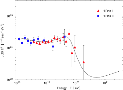
Figure 1: UHECR spectrum and HiRes observations. The figure shows the UHECR spectrum $J(E)$ multiplied by $E^{3}$, for uniform distributed sources, without evolution ($m=0$), generation index $\gamma_{g}=2.7$, and with a maximum generation energy $E_{\mathrm{max}}=\infty$. Also shown are the HiRes observed events.

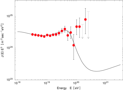
Figure 2: UHECR spectrum and AGASA observations. The figure shows the UHECR spectrum $J(E)$ multiplied by $E^{3}$, for uniform distributed sources, without evolution, and with a maximum generation energy $E_{\mathrm{max}}=\infty$. Also shown are the AGASA observed events. The best fit for the low energy sector ($E<4\times 10^{19}$ eV) corresponds to $\gamma_{g}=2.7$.

Fig.1 shows the obtained spectrum $J(E)$ of UHECR and the HiRes observed data (two detectors, HiRes-I and HiRes-II). In order to emphasize the appearance of the GZK-cutoff in the spectrum, we have selected the idealized case when the maximum generation energy $E_{\mathrm{max}}$ for the emitted particles from sources, is $E_{\mathrm{max}}=\infty$. To fit the HiRes data, the generation index for the theoretical spectrum shown in the figure is $\gamma_{g}=2.7$, while the evolution index is $m=0$. Additionally, the volumetric luminosity is $\mathcal{L}_{0}=2.96\times 10^{51}\mathrm{ergs}/\mathrm{Mpc}^{3}\mathrm{yr}$.

Fig.2 shows the obtained spectrum $J(E)$ of UHECR and the AGASA observed data. Again, we have selected for the theoretical spectrum $J(E)$ the idealized case $E_{\mathrm{max}}=\infty$. To reconcile the data of the low energy region ($E<4\times 10^{19}$ eV), where the pair creation dominates the energy loss, it is necessary to have a generation index $\gamma_{g}=2.7$ (with the additional supposition that sources do not evolve) and a volumetric luminosity $\mathcal{L}_{0}=4.7\times 10^{51}\mathrm{ergs}/\mathrm{Mpc}^{3}\mathrm{yr}$. It can be seen that for events with energies $E>4\times 10^{19}$ eV, where the energy loss is dominated by the photo-pion production, the predicted spectrum does not fit the data well. To have a statistical sense of the discrepancy between observation and theory, we can calculate the Poisson probability $P$ of an excess in the five highest energy bins. This is $P=1.1\times 10^{-8}$. Another statistical measure is provided by the Poisson $\chi^{2}$ given by PDG

$$\chi^{2}=\sum_{i}[2(N_{i}^{\mathrm{th}}-N_{i}^{\mathrm{obs}})+2N_{i}^{\mathrm{obs}}\ln(N_{i}^{\mathrm{obs}}/N_{i}^{\mathrm{th}})].$$ (31)

Computing this quantity for the eight highest energy bins, we obtain $\chi^{2}=29$. These quantities show how far the AGASA measurements are from the theoretical prediction given by the curve of Fig.2. Other more sophisticated models have also been analyzed in detail Berezinsky , nevertheless, it has turned out that conventional physics does not have the capacity to reproduce the observations from the AGASA collaboration group in a satisfactory way.

Whether HiRes or AGASA data are pointing in the right direction to describe the correct pattern present in the arrival of UHECR is still an open issue (see, for example, reference MBO for a detailed comparison between both experimental results). In the rest of the paper we shall focus our attention on the possibility of an absence of the GZK cutoff as a consequence of LQG effects. For this reason, we will later return to the AGASA observations in order to contrast the results of the following sections.

III Loop Quantum Gravity

Loop quantum gravity is a canonical approach to the problem of gravity quantization. It is based on the construction of a spin network basis, labelled by graphs embedded in a three dimensional insertion $\Sigma$ in space-time. A consequence of this approach is that the quantum structure of space-time will be of a polymer-like nature, highly manifested in phenomena involving the Planck scale $l_{p}$.

The above, and very brief outline of loop quantum gravity allows us to figure out how complicated a full treatment of a physical phenomena could be when the quantum nature of gravity is considered, even if the physical system is characterized by a flat geometry. It is possible, however, to introduce a loop state which approximates a flat 3-metric on $\Sigma$ at length scales greater than the length scale $\mathcal{L}\gg l_{p}$. For pure gravity, this state is referred to as the weave state $|W\rangle$, and the length scale $\mathcal{L}$ as the weave scale. A flat weave $|W\rangle$ will be characterized by $\mathcal{L}$ in such a way that for distances $d\ll\mathcal{L}$ the quantum loop structure of space is manifest, while for distances $d\geqslant\mathcal{L}$ the continuous flat geometry is regained. With this approach, for instance, the metric operator $\hat{q}_{ab}$ satisfies

$$\langle W|\hat{q}_{ab}|W\rangle=\delta_{ab}+\mathcal{O}(l_{p}/\mathcal{L}).$$ (32)

A generalization of the former idea, to include matter fields, is also possible. In this case, the loop state represents a matter field $\psi$ coupled to gravity. Such a state is denoted by $|W,\psi\rangle$ and, again, is simply referred to as the weave. As before, it will be characterized by the weave scale $\mathcal{L}$ and the hamiltonian operators $\hat{H}_{\psi}$ are expected to fulfill a relation analog to (32), that is, we shall be able to define an effective hamiltonian $H_{\psi}$ such that

$$H_{\psi}=\langle W,\psi|\hat{H}_{\psi}|W,\psi\rangle.$$ (33)

An approach to this task has been performed by J. Alfaro et al. Neutrinos ; Photons ; AMU for 1/2-spin fermions and the electromagnetic field. In this approach the effects of the loop structure of space at the Planck level are treated semiclassically through a coarse-grained approximation Gambini Pullin . This method leads to the natural appearance of LIV’s in the equations of motion derived from the effective hamiltonian. The key feature here is that the effective hamiltonian is constructed from expectation values of dynamical quantities from both the matter fields and the gravitational field. In this way, when a flat weave is considered, the expectation values of the gravitational part will appear in the equations of motion for the matter fields in the form of coefficients with dependence in both scales, $\mathcal{L}$ and $l_{p}$. When a flat geometry is considered, the expectation values can be interpreted as vacuum expectation values for the considered matter fields.

A significant discussion is whether the Lorentz symmetry is present in the full LQG theory (as in its classical counterpart) or not Thiemann1 . For the present work, we shall assume that Lorentz symmetry is indeed present in the full LQG theory. This assumption, jointly with the consideration that the new corrective coefficients are vacuum expectation values, leads us to consider that the Lorentz symmetry is spontaneously broken in the effective theory level.

In what follows we will briefly summarize the obtained equations of motion for both, 1/2-spin fermions and photons, as well as the obtained dispersion relations.

III.1 Fermions

The LQG effective equations of motion for a $1/2$-spin fermion field, coupled to gravity, are Neutrinos

$$\left[i\frac{\partial}{\partial t}-i\hat{A}\vec{\sigma}\cdot\nabla+\frac{\hat{B}}{2\mathcal{L}}\right]\xi(x)\qquad\qquad\qquad$$

$$-m(C-iD\vec{\sigma}\cdot\nabla)\chi(x)=0,$$ (34)

$$\left[i\frac{\partial}{\partial t}+i\hat{A}\vec{\sigma}\cdot\nabla-\frac{\hat{B}}{2\mathcal{L}}\right]\chi(x)\qquad\qquad\qquad$$

$$-m(C-iD\vec{\sigma}\cdot\nabla)\xi(x)=0,$$ (35)

where $\xi(x)$ and $\chi(x)$ are the spinor components for the Dirac field $\Psi(x)=(\xi(x),\chi(x))$ and the hermitian operators, $\hat{A}$ and $\hat{C}$, are given by the following expressions

$$\hat{A} = 1+\kappa_{1}\frac{l_{p}}{\mathcal{L}}+\kappa_{2}\left(\frac{l_{p}}{\mathcal{L}}\right)^{2}+\frac{\kappa_{3}}{2}l_{p}^{2}\nabla^{2},$$ (36)

$$\hat{B} = \kappa_{5}\frac{l_{p}}{\mathcal{L}}+\kappa_{6}\left(\frac{l_{p}}{\mathcal{L}}\right)^{2}+\frac{\kappa_{7}}{2}l_{p}^{2}\nabla^{2},$$ (37)

and the constants $C$ and $D$ are given by

$$C = 1+\kappa_{8}\frac{l_{p}}{\mathcal{L}},$$ (38)

$$D = \frac{\kappa_{9}}{2\hbar}l_{p}.$$ (39)

In the above expressions the $\kappa_{i}$ quantities are unknown coefficients of order 1 which need to be determined. In the case that $\Psi(x)$ is a Majorana field, the $\xi(x)$ and $\chi(x)$ spinors fulfill the reality condition:

$$\xi(x)=-i\sigma^{2}\,\chi^{*}(x)\quad\mathrm{and}\quad\chi(x)=i\sigma^{2}\,\xi^{*}(x).$$ (40)

With the help of this condition, equations (34) and (35) can be simplified to

$$\left[\frac{\partial}{\partial t}-\hat{A}\vec{\sigma}\cdot\nabla-\frac{i\hat{B}}{2\mathcal{L}}\right]\xi(x)\qquad\qquad\qquad$$

$$-m(C-iD\vec{\sigma}\cdot\nabla)\sigma^{2}\xi^{*}(x)=0.$$ (41)

Equations (34) and (35) are invariant under charge conjugation C and time inversion T, but not under parity conjugation P. As a consequence, the fermion equation of motion violates the CPT symmetry through P. The terms that produce the P violation are those related with $\hat{B}$ and $D$.

Some comments need to be made at this stage. Of specially importance to the development of the above effective equations of motion is that they are only valid in a homogenous and isotropic system. From the point of view of a spontaneous symmetry breakup such a system is unique and, therefore, a privileged reference frame). It is possible then to put the equations of motion (and therefore the dispersion relations) in a covariant form through the introduction of a four-velocity vector explicitly denoting the existence of a preferred system. From the cosmological point of view, such a privileged system does exist, and corresponds to the CMBR co-moving reference system. For that reason, we shall assume that the preferred system denoted by the presence of LIV’s is the same CMBR co-moving reference frame, and will use it as the laboratory system.

The dispersion relation for fermions can be easily obtained through the development of the Klein-Gordon-like equation. The obtained dispersion relation is

$$E_{\pm}^{2}=(Ap\pm\frac{B}{2\mathcal{L}})^{2}+m^{2}(C\pm Dp)^{2}$$ (42)

where the $\pm$ signs correspond to the helicity state of the described particle (note that these signs are produced by the parity violation coefficients), and where now we have

$$A = 1+\kappa_{1}\frac{l_{p}}{\mathcal{L}}+\kappa_{2}\left(\frac{l_{p}}{\mathcal{L}}\right)^{2}+\frac{\kappa_{3}}{2}l_{p}^{2}p^{2},$$

$$B = \kappa_{5}\frac{l_{p}}{\mathcal{L}}+\kappa_{6}\left(\frac{l_{p}}{\mathcal{L}}\right)^{2}+\frac{\kappa_{7}}{2}l_{p}^{2}p^{2},$$

$$C = 1+\kappa_{8}\frac{l_{p}}{\mathcal{L}},$$

$$D = \frac{\kappa_{9}}{2}l_{p}.$$ (43)

For our purposes, it will be sufficient to consider the lower contributions in both scales, $l_{p}$ and $\mathcal{L}$ Alfaro & Palma

$$E^{2}_{\pm}=p^{2}+2\alpha p^{2}+\eta p^{4}\pm 2\lambda p+m^{2},$$ (44)

where we have defined the new set of corrections $\alpha$, $\eta$ and $\lambda$ depending on the scales $\mathcal{L}$ and $l_{p}$ in the following way:

$$\alpha = \kappa_{\alpha}(l_{p}/\mathcal{L})^{2}$$ (45)

$$\eta = \kappa_{\eta}\,l_{p}^{2}$$ (46)

$$\lambda = \kappa_{\lambda}\,l_{p}/2\mathcal{L}^{2},$$ (47)

being $\kappa_{\alpha}$, $\kappa_{\eta}$ and $\kappa_{\lambda}$ adimensional parameters of order 1.

III.2 Photons

For the electromagnetic sector of the theory we have the following set of effective equations

$$A(\nabla\times\vec{B})-\frac{1}{c}\frac{\partial\vec{E}}{\partial t}+2l_{p}^{2}\theta_{3}\nabla^{2}(\nabla\times\vec{B})$$

$$-2\theta_{8}l_{p}\nabla^{2}\vec{B}+4\theta_{4}\mathcal{L}^{2}\left(\frac{\mathcal{L}}{l_{p}}\right)^{2\Upsilon}l_{p}^{2}\nabla\times(\vec{B}^{2}\vec{B})=0,$$ (48)

$$A(\nabla\times\vec{E})+\frac{1}{c}\frac{\partial\vec{B}}{\partial t}+2l_{p}^{2}\theta_{3}\nabla^{2}(\nabla\times\vec{E})$$

$$-2\theta_{8}l_{p}\nabla^{2}\vec{E}=0,$$ (49)

where

$$A=1+\theta_{7}\left(\frac{l_{p}}{\mathcal{L}}\right)^{2+2\Upsilon}.$$ (50)

To calculate a dispersion relation for photons we need to consider only the linear part of equations (48) and (49), and try solutions of the type $\vec{E}=\vec{E}_{0}e^{i(\vec{k}\cdot\vec{x}-\omega t)}$ and $\vec{B}=\vec{B}_{0}e^{i(\vec{k}\cdot\vec{x}-\omega t)}$, for the electric and magnetic fields. In this way, the obtained dispersion relation between the energy $\omega$ and the momentum $k$ of photons is

$$\omega_{\pm}=k[A_{\gamma}-\theta_{3}(l_{p}k)^{2}\pm\theta_{8}l_{p}k],$$ (51)

where

$$A_{\gamma} = 1+\kappa_{\gamma}\left(\frac{l_{p}}{\mathcal{L}}\right)^{2+2\Upsilon}.$$ (52)

In the previous expression the $\kappa_{\gamma}$ and $\theta_{i}$ coefficients are adimensional parameters of order 1. As before, the $\pm$ signs refer to the helicity state of the described photons. The $\Upsilon$ quantity is a free parameter that measures a possible non-canonical scaling of the gravitational expectation values in the semiclassical state (let us note that the presence of $\Upsilon$ in the fermionic sector was not considered in Neutrinos ). To be consistent with the dispersion relation of fermions, we shall consider only possibilities $\Upsilon$ = -1/2, 0, 1/2, 1, etc., in such a way that $A_{\gamma}\sim 1+\mathcal{O}[(l_{p}/\mathcal{L})^{n}]$, where $n=2+2\Upsilon$ is a positive natural number. With this supposition, we can find a tentative value for $\Upsilon$, through the bound of the lower order correction $\delta A\sim\mathcal{O}[(l_{p}/\mathcal{L})^{n}]$ (where $\delta A=A_{\gamma}-A_{a}$, being $a$ another particle).

Considering the lower order contributions in both scales, $l_{p}$ and $\mathcal{L}$, we are able to simplify the photon dispersion relation to

$$\omega^{2}_{\pm}=k^{2}+2\alpha_{\gamma}k^{2}\pm 2\theta_{\gamma}l_{p}k^{3},$$ (53)

where $\alpha_{\gamma}$ is defined by the relation $A_{\gamma}=1+\alpha_{\gamma}=1+\kappa_{\gamma}\,(l_{p}/\mathcal{L})^{2+2\Upsilon}$.

III.3 Other Particles

We have so far examined the dispersion relations coming from LQG for both $1/2$-spin fermions and photons. A relevant issue for the following developments is the establishment of a valid extension of the former results for other particles. In particular, we are interested in counting with dispersion relations for 3/2-spin fermions and 0-spin massive bosons. A precise and rigorous procedure would require a complete calculation of effective field equations of motion coming from LQG for each particle flavor in which we are interested. For present purposes we will assert that the valid dispersion relation for more general fermions is simply

$$E^{2}_{\pm}=p^{2}+2\alpha p^{2}+\eta p^{4}\pm 2\lambda p+m^{2},$$ (54)

This assertion preserves the basic symmetries and assumptions that have lead to the obtention of the equations of motion for 1/2-spin fermions.

On the other hand, in the case of bosonic 0-spin particles, we will assert that the valid dispersion relation consists of

$$E^{2}=p^{2}+2\alpha p^{2}+\eta p^{4}+m^{2}.$$ (55)

This assertion is based on the fact that the symmetries involved in the construction of the effective hamiltonian for 0-spin bosons would prevent the appearance of terms like $\lambda$ (which depends on the helicity).

To conclude, let us mention that the dispersion relation (54) will be used for the physical description of electrons, protons, neutrons, and $\Delta$ and $N$ baryonic resonances. Meanwhile, the dispersion relation (55) will be used for mesons $\pi$, $\rho$ and $\omega$.

IV Threshold Conditions

A useful discussion around the effects that LIV’s can have on the propagation of UHECR can be raised through the study of the threshold conditions for the reactions to take place Coleman & Glashow . To simplify our subsequent discussions, let us use the following notation for the modified dispersion relations

$$E^{2}=p^{2}+f(p)+m^{2},$$ (56)

where $f(p)$ is the deformation function of the momentum $p$.

A decay reaction is kinematically allowed when, for a given value of the total momentum $\vec{p}_{0}=\sum_{\mathrm{initial}}\vec{p}=\sum_{\mathrm{final}}\vec{p}$, one can find a total energy value $E_{0}$ such that $E_{0}\geqslant E_{\mathrm{min}}$. Here $E_{\mathrm{min}}$ is the minimum value attainable by the total energy of the decaying products for a given total momentum $\vec{p}_{0}$. To find $E_{\mathrm{min}}$, it is enough to take the individual decay product momenta to be collinear with respect to the total momentum $\vec{p}_{0}$ and with the same direction. To see this, we can variate $E_{0}$ with the appropriate restrictions

$$E_{0}=\sum_{i}E_{i}(p_{i})+\xi_{j}(p_{0}^{\,j}-\sum_{i}p_{i}^{\,j}),$$ (57)

where $\xi_{j}$ are Lagrange multipliers, the $i$ index specifies the $i$th particle and the $j$ index the $j$th vectorial component of the different quantities. Doing the variation, we obtain

$$\frac{\partial E_{i}}{\partial p_{i}^{j}}\equiv v_{i}^{j}=\xi_{j}.$$ (58)

That is to say, the velocities of all the final produced particles must be equal to $\xi$. Since the dispersion relations that we are treating are monotonously increasing in the range of momenta $p>\lambda$, the momenta can be taken as being collinear and with the same direction of the initial quantity $\vec{p}_{0}$.

In this work, we will focus on those cases in which two particles (say $a$ and $b$) collide to subsequently decay in the aforementioned final states. For the present discussion, particles $a$ and $b$ have momenta $\vec{p}_{a}$ and $\vec{p}_{b}$ respectively, and the total momentum of the system is $\vec{p}_{0}$. It is easy to see from the dispersion relations that we are considering, that the total energy of the system will depend only on $p_{a}=|\vec{p}_{a}|$ and $p_{b}=|\vec{p}_{b}|$. Therefore, to obtain the threshold condition for the mentioned kind of process, we must find the maximum possible total energy $E_{\mathrm{max}}$ of the initial configuration, given the knowledge of $p_{a}$ and $p_{b}$. To accomplish this, let us fix $\vec{p}_{a}$ and variate the incoming direction of $\vec{p}_{b}=\hat{n}p_{b}$ in

$$E_{0} = E_{a}(\vec{p}_{0}-p_{b}\hat{n})+E_{b}(p_{b})+\chi(\hat{n}^{2}-1).$$ (59)

Varying (59) with respect to $\hat{n}$ ($\chi$ is a Lagrange multiplier), we find

$$\hat{n}^{i}=\frac{v_{a}^{i}p_{b}}{2\chi}.$$ (60)

In this way we obtain two extremal situations $\chi=\pm v_{a}p_{b}/2$, or simply

$$\hat{n}^{i}=\pm\frac{v_{a}^{i}}{v_{a}}.$$ (61)

A simple inspection shows that for the dispersion relations that we are considering, the maximum energy is given by $\hat{n}^{i}=-v_{a}^{i}/v_{a}$, or in other words, when a frontal collision takes place.

Summarizing the threshold condition for a two particle ($a$ and $b$) collision and subsequent decay, can be expressed through the following requirements:

$$E_{a}+E_{b}\geqslant\sum_{\mathrm{final}}E_{f},$$ (62)

with all final particles having the same velocity ($v_{i}=v_{j}$ for any to final particles $i$ and $j$), and

$$p_{a}-p_{b}=\sum_{\mathrm{final}}p_{f},$$ (63)

where the sign of the momenta $\sum_{\mathrm{final}}p_{f}$ is given by the direction of the highest momentum magnitude of the initial particles.

Our interest in the next subsections is the study of the reactions involved in high energy cosmic ray phenomena through the threshold conditions. To accomplish this goal through simple expressions that are easy-to-manipulate, we shall further use, for the equal velocities condition, the simplification

$$E_{b}m_{a}=E_{a}m_{b},$$ (64)

valid for the study of parameters coming from the region $f(p)\ll m^{2}$. This simplification will allow the achievement of bounds over the order of magnitude of the different parameters involved in the modified dispersion relations, which are precisely our main concern.

In the following subsections we will study the kinematical effects of LIV’s through the threshold conditions for the reactions involved in the propagation of UHECR. Since, in this phenomena, photons are present in the form of low energy particles (the soft photons of the CMBR), the LQG corrections in the electromagnetic sector of the theory can be ignored. LQG corrections to the electromagnetic sector, however, have already been studied for other high energy reactions such as the Mkn 501 $\gamma$-rays Alfaro & Palma .

IV.1 Photo-Pion Production $\gamma+p\rightarrow p+\pi$

Let us begin with the photo-pion production $\gamma+p\rightarrow p+\pi$. Considering the corrections provided in the dispersion relations (44) and (55) for fermions and bosons, we note that, for the photo-pion production to proceed, the following condition must be satisfied

$$2\,\delta\alpha\,E_{\pi}^{2}+\left(\delta\eta+3\eta_{p}\frac{m_{p}(m_{p}+m_{\pi})}{m_{\pi}^{2}}\right)E_{\pi}^{4}$$

$$+2E_{\pi}(|\lambda_{p}|\pm\lambda_{p})+4E_{\pi}\omega\geqslant\frac{m_{\pi}^{2}(2m_{p}+m_{\pi})}{m_{p}+m_{\pi}},$$ (65)

where $E_{\pi}$ is the energy of the emergent pion, $\delta\alpha=\alpha_{p}-\alpha_{\pi}$ and $\delta\eta=\eta_{p}-\eta_{\pi}$. In expression (IV.1), the $\pm$ signs refer to the helicity of the incident proton. Since there will necessarily be a proton helicity that can minimize the term associated with $\lambda_{p}\,$ and, therefore, minimize the energy configuration for the threshold condition, we must insert, in (IV.1), the following equality

$$2E_{\pi}(|\lambda_{p}|\pm\lambda_{p})=0.$$ (66)

In addition, we are assuming that the difference between $\kappa$ parameters from different particles are of order 1 ($\delta\kappa\sim 1$). Therefore, if not null, we can take $\eta_{p}$ to dominate over $\delta\eta$ in (IV.1). With these considerations in mind, we are left with

$$2\,\delta\alpha\,E_{\pi}^{2}+168\eta_{p}E_{\pi}^{4}+4E_{\pi}\omega\geqslant\frac{m_{\pi}^{2}(2m_{p}+m_{\pi})}{m_{p}+m_{\pi}}.$$ (67)

Note that in the absence of LQG corrections, the threshold condition is simply

$$4E_{\pi}\omega\geqslant\frac{m_{\pi}^{2}(2m_{p}+m_{\pi})}{m_{p}+m_{\pi}}.$$ (68)

IV.2 Resonant Production $\gamma+p\rightarrow\Delta$

The main channel involved in the photo-pion production is the resonant production of the $\Delta(1232)$. It can be shown that the threshold condition for the resonant $\Delta(1232)$ decay reaction to occur, is

$$2\,\delta\alpha\,E_{p}^{2}+\delta\eta\,E_{p}^{4}+2\left[(\pm)_{p}\,\lambda_{p}+|\lambda_{\Delta}|\,\right]E_{p}$$

$$+4\omega E_{p}\geqslant m_{\Delta}^{2}-m_{p}^{2}\,,$$ (69)

where $E_{p}$ is the incident proton energy, $\delta\alpha=\alpha_{p}-\alpha_{\Delta}$ and $\delta\eta=\eta_{p}-\eta_{\Delta}$. Additionally, $(\pm)_{p}$ refers to the incident proton helicity. In the absence of LQG corrections, the conventional threshold condition is naturally reobtained:

$$E_{p}\geqslant\frac{m_{\Delta}^{2}-m_{p}^{2}}{4\omega}.$$ (70)

IV.3 Pair Creation $\gamma+p\rightarrow p+e^{+}+e^{-}$

Pair creation, $\gamma+p\rightarrow p+e^{+}+e^{-}$, is greatly abundant in the sector previous to the GZK limit. When the dispersion relations for fermions are considered for both protons and electrons, it is possible to find

$$\delta\alpha\frac{m_{e}}{m_{p}+2m_{e}}E^{2}\qquad\qquad\qquad\qquad\qquad\qquad\qquad$$

$$+2\left(\delta\eta+\frac{3}{4}\eta_{p}\frac{m_{p}(m_{p}+2m_{e})}{m_{e}^{2}}\right)\left(\frac{m_{e}}{m_{p}+2m_{e}}\right)^{3}E^{4}$$

$$+E\omega+|\lambda_{e}|E+\frac{1}{2}(|\lambda_{p}|\pm\lambda_{p})E\geqslant m_{e}(m_{p}+m_{e}),$$ (71)

with $\delta\alpha=\alpha_{p}-\alpha_{e}$ and $\delta\eta=\eta_{p}-\eta_{e}$.

As in the case of photo-pion production, there will always be an incident proton helicity which can minimize the inequality (IV.3). Therefore, to study the production of the electron-positron pair under its threshold condition, we shall set $|\lambda_{p}|\pm\lambda_{p}=0$. On the other hand, since our intention is to estimate an order of magnitude for the value of the diverse parameters present in the theory, let us ignore the $\delta\eta$ term, since the presence of $\eta_{p}$ is of greater relevance (recall that we are considering that $\mathcal{O}(\eta)=\mathcal{O}(\delta\eta)$). With these considerations, we obtain

$$\delta\alpha\,\frac{m_{e}}{m_{p}}E^{2}+\frac{3}{2}\eta\frac{m_{e}}{m_{p}}E^{4}+|\lambda_{e}|E$$

$$+E\omega\geqslant m_{e}(m_{p}+m_{e}),$$ (72)

where we have also used $m_{p}+m_{e}\simeq m_{p}$, to simplify the above expression.

Finally, if no corrections are present at all, the threshold condition would be reduced to the conventional one,

$$E\omega\geqslant m_{e}(m_{p}+m_{e}).$$ (73)

IV.4 Bounds

In order to study the threshold conditions (67), (IV.2) and (IV.3), in the context of the GZK anomaly, we must establish some criteria.

Firstly, as we have seen in section II, the conventionally obtained theoretical spectrum provides a very good description of the phenomena up to an energy $\sim 4\times 10^{19}$ eV. The main reaction taking place in this well described region is the pair creation $\gamma+p\rightarrow p+e^{+}+e^{-}$ and, therefore, no modifications are present for this reaction up to $\sim 4\times 10^{19}$ eV. As a consequence, and since threshold conditions offer a measure of how modified kinematics is, we will require that the threshold condition (IV.3) for pair creation not be substantially altered by the new corrective terms.

Secondly, we have the GZK anomaly itself, which we are committed to explain. Since for energies greater than $\sim 8\times 10^{19}$ eV the conventional theoretical spectrum does not fit the experimental data well, we shall require that LQG corrections be able to offer a violation of the GZK-cutoff. The dominant reaction in the violated $E>8\times 10^{19}$ region is the photo-pion production and, therefore, we shall require further that the new corrective terms present in the kinematical calculations be able to shift the threshold significantly to preclude the reaction.

As a last possibility, we shall also examine the bounds arising for the case in which no GZK anomaly (and therefore no violations to the threshold and kinematics) really exists. Since the HiRes data have reached the $\sim 1.8\times 10^{20}$ eV, we will consider the scenario in which no violation at all is confirmed by the data up to a reference energy $E_{\mathrm{ref}}=2\times 10^{20}$ eV.

In order to study the different corrections, given that we don’t have a detailed knowledge of the deviation parameters, we shall take account of them independently. Naturally, there will always exist the possibility of having an adequate combination of these parameter values that could affect the threshold conditions simultaneously. However, as shall soon be evident, each one of these parameters will be significant at different energy ranges.

IV.4.1 $\alpha$ Correction

We shall begin our analysis with correction $\alpha$ and the consideration of the threshold condition for pair production. In this case we have

$$\delta\alpha\,\frac{m_{e}}{m_{p}}E^{2}+E\omega\geqslant m_{e}(m_{p}+m_{e}),$$ (74)

with $\delta\alpha=\alpha_{p}-\alpha_{e}$. As is clear from the above condition, the minimum soft-photon energy $\omega_{\mathrm{min}}$ for the pair production to occur, is

$$\omega_{\mathrm{min}}=\frac{m_{e}}{E}(m_{p}+m_{e})-\delta\alpha\,\frac{m_{e}}{m_{p}}E.$$ (75)

It follows therefore that the condition for a significant increase or decrease in the threshold energy for pair production becomes $|\delta\alpha|\geqslant m_{p}(m_{p}+m_{e})/E^{2}$. In this way, if we do not want kinematics to be modified up to a reference energy $E_{\mathrm{ref}}=3\times 10^{19}$, we must impose the following constraint

$$|\alpha_{p}-\alpha_{e}|<\frac{(m_{p}+m_{e})m_{p}}{E_{\mathrm{ref}}^{2}}=9.8\times 10^{-22}.$$ (76)

Similar treatments can be found for the analysis of other astrophysical signals like the Mkn 501 $\gamma$-rays Stecker & Glashow , when the absence of anomalies is considered.

Let us now consider the threshold condition for the photo-pion production. Taking only the $\alpha$ correction, we have

$$2\,\delta\alpha\,E_{\pi}^{2}+4E_{\pi}\omega\geqslant\frac{m_{\pi}^{2}(2m_{p}+m_{\pi})}{m_{p}+m_{\pi}}.$$ (77)

It is possible to find that for the above condition to be violated for all energies $E_{\pi}$ of the emerging pion, and therefore no reaction to take place, the following inequality must hold

$$\alpha_{\pi}-\alpha_{p}>\frac{2\omega^{2}(m_{p}+m_{\pi})}{m_{\pi}^{2}(2m_{p}+m_{\pi})}=3.3\times 10^{-24}\left[\omega/\omega_{0}\right]^{2}.$$ (78)

where $\omega_{0}=KT=2.35\times 10^{-4}$ eV is the thermal CMBR energy. If we repeat these steps for the $\Delta(1232)$ resonant decay, we obtain the following condition

$$\alpha_{\Delta}-\alpha_{p}>\frac{2\omega^{2}}{m_{\Delta}^{2}-m_{p}^{2}}=1.7\times 10^{-25}\left[\omega/\omega_{0}\right]^{2}.$$ (79)

To estimate a range for the weave scale $\mathcal{L}$, let us use as a reference energy $\omega_{\mathrm{ref}}=\omega_{\mathrm{min}}$, where $\omega_{\mathrm{min}}$ is the minimum energy for the reaction to take place, in inequality (77), when the condition for a significant increase in the threshold condition is taken into account (for a primordial proton reference energy $E_{\mathrm{ref}}=2\times 10^{20}$, this is $\omega_{\mathrm{min}}\sim 2.9\times\omega_{0}$), and join the results deduced from the mentioned requirements. Assuming that the $\kappa_{\alpha}$ parameters are of order 1, as well as the difference between them for different particles, we can estimate —for the weave scale $\mathcal{L}$— the preferred range

$$2.6\times 10^{-18}\,\,\,\mathrm{eV}^{-1}\lesssim\mathcal{L}\lesssim 1.6\times 10^{-17}\,\,\,\mathrm{eV}^{-1},$$ (80)

where the lefthand and righthand sides come from bounds (76) and (78) respectively (since the $\Delta$(1232) is just one channel of the photo-pion production, we shall not consider it to set any bound).

If no GZK anomaly is confirmed in future experimental observations, then we should state a stronger bound for the difference $\alpha_{\pi}-\alpha_{p}$. Using the same assumptions to set the restriction (76) when the primordial proton reference energy is $E_{\mathrm{ref}}=2\times 10^{20}$ eV, it is possible to find

$$|\alpha_{\pi}-\alpha_{p}|<2.3\times 10^{-23}.$$ (81)

In terms of the length scale $\mathcal{L}$, this last bound may be read as

$$\mathcal{L}\gtrsim 1.7\times 10^{-17}\,\,\mathrm{eV}^{-1},$$ (82)

which is a stronger bound over $\mathcal{L}$ than (76), offered by pair creation.

IV.4.2 $\eta$ Correction

Let us now turn our attention to the $\eta$ parameter. The threshold condition for the pair production, when only the $\eta$ parameter is considered, is

$$\frac{3}{2}\eta\frac{m_{e}}{m_{p}}E^{4}+E\omega\geqslant m_{e}(m_{p}+m_{e}).$$ (83)

Repeating the same analysis we did for the $\alpha$ parameter, it is possible to find the following constraint

$$|\eta|<\frac{2}{3}\frac{m_{p}}{E_{\mathrm{ref}}^{4}}(m_{p}+m_{e})=1.6\times 10^{-60}\,\,\mathrm{eV}^{-2}.$$ (84)

Recalling that $\eta=\kappa_{\eta}l_{p}^{2}$, result (84) can be reexpressed in the form

$$|\kappa_{\eta}|\lesssim 2.4\times 10^{-4},$$ (85)

which is, of course, a strong bound over a parameter of order 1.

Since the basis of the effective LQG methods which we have developed rely on the fact that the coefficients $\kappa$ are of order 1, we must conclude that a reaction of the type $\eta$ should be discarded, in opposition to the expectations of our previous work Alfaro & Palma , when only photo-pion production was analyzed.

IV.4.3 $\lambda$ Correction

Finally we have to consider the $\lambda$ correction. In our previous work Alfaro & Palma , having studied the photo-pion production through the $\Delta(1232)$ channel decay, we emphasized the possibility of a helicity dependent violation. For this effect to take place, the following configuration must be satisfied (using again $\omega_{\mathrm{ref}}=\omega_{\mathrm{min}}$)

$$|\lambda_{p}|\geqslant|\lambda_{\Delta}|+1.3\times 10^{-3}\,\,\mathrm{eV}.$$ (86)

However, when pair production is analyzed (in the same way as with $\alpha$ and $\eta$), the following condition emerges for $\lambda_{e}$:

$$|\lambda_{e}|<1.6\times 10^{-5}\,\,\mathrm{eV},$$ (87)

which is more than 1 order of magnitude stronger than the required value for protons in (86). This weakens the possibility of a limit violation through helicity dependent effects.

Another stronger bound can be found in Carmona Cortes , where a dispersion relation of the type

$$E^{2}=p^{2}+\lambda p+m^{2}$$ (88)

is analyzed, and it is found that the case $\lambda\geqslant 1\times 10^{-7}$ eV should be discarded because of the highly sensitive measurements of the Lamb shift.

IV.5 The Cubic Correction

A commonly studied correction which has appeared in several recent works Amelino ; Ellis ; Liberati1 , and which deserves our attention, is the case of a cubic correction of the form

$$E^{2}=p^{2}+m^{2}+\xi\,p^{3},$$ (89)

(where $\xi$ is an arbitrary scale). It is interesting to note that strong bounds can be placed over deformation $f(p)=\xi\,p^{3}$. We will assume in this section, that $\xi$ is an universal parameter (an assumption followed by most of the works in this field).

¿From dispersion relation (89), the threshold condition for the photo-pion production is

$$4\,\omega E+2\,\xi\frac{m_{\pi}m_{p}}{(m_{p}+m_{\pi})^{2}}E^{3}\geqslant m_{\pi}(2m_{p}+m_{\pi}).$$ (90)

Clearly, when $\xi$ is negative, it can be observed from (90) that the threshold energy for photo-pion production can be easily shifted, preventing the reaction to take place for high energies. The condition for this to be the case is

$$-\xi > \frac{128}{27}\frac{\omega_{0}^{3}}{m_{\pi}^{3}m_{p}}\left(\frac{m_{p}+m_{\pi}}{2m_{p}+m_{\pi}}\right)^{2}[\omega/\omega_{0}]^{3}$$ (91)

$$=7.75\times 10^{-45}\,[\omega/\omega_{0}]^{3}\,\,\mathrm{eV}^{-1}.$$

It can be seen therefore that in the particular case of $\xi=-l_{p}$ ($l_{p}=8.3\times 10^{-29}$ eV^-1), the reaction can be considerably suppressed.

Let us note, however, that the pair production $p+\gamma\rightarrow p+e^{+}+e^{-}$ imposes strong restrictions over a negative $\xi$ parameter. Following the methods that we have used up to now, it is possible to find that the threshold condition for the pair production is

$$\omega E+\xi\frac{m_{e}m_{p}}{(m_{p}+2m_{e})^{2}}E^{3}\geqslant m_{e}(m_{p}+m_{e}).$$ (92)

Since we cannot infer modifications in the description of pair production in the cosmic ray spectra up to energies $E\sim 4\times 10^{19}$ eV, we must at least impute the following inequality

$$|\xi| < \frac{(m_{p}+m_{e})(m_{p}+2m_{e})^{2}}{m_{p}\,E_{\mathrm{ref}}^{3}}$$ (93)

$$=3.26\times 10^{-41}\,\,\mathrm{eV}^{-1}$$

$$(=3.98\times 10^{-13}\,l_{p}),$$

where we have used $E_{\mathrm{ref}}=3\times 10^{19}$ eV. This last result shows the strong suppression over $\xi\,$. As a consequence, the particular case $|\xi|=l_{p}=8\times 10^{-28}$ eV^-1 should be discarded. A bound like (93) seems to have been omitted up to now for the GZK anomaly analysis.

V Modified Spectrum

In this section we shall show how the only surviving LQG correction from our previous analysis in section IV, $A=1+\alpha$, can affect the prediction of the theoretical cosmic ray spectrum. Our approach will be centered on the supposition that the LQG corrections to the main quantities for the calculation —such as cross sections and inelasticities of processes— are, in a first instance, kinematical corrections, and that the Lorentz symmetry is spontaneously broken. These assumptions will allow us to introduce the adequate corrections when a modified dispersion relation is known.

V.1 Kinematics

When having a spontaneous Lorentz symmetry breaking, we can use the still valid Lorentz transformations to express physical quantities observed in one reference system, in another one. This is possible since, under a spontaneous symmetry breaking, the group representations of the broken group preserves its transformation properties. In particular, it will be possible to relate the observed 4-momenta in different reference systems through the usual rule

$$p_{\mu}^{\prime}=\Lambda_{\mu}^{\,\,\,\nu}p_{\nu},$$ (94)

where $p_{\mu}=(-E,\vec{p})$ is an arbitrary 4-momentum expressed in a given reference system $\mathcal{K}$, $p_{\mu}^{\prime}$ is the same vector expressed in another given system $\mathcal{K}^{\prime}$, and $\Lambda_{\mu}^{\,\,\,\nu}$ is the usual Lorentz transformation connecting both systems. Such a transformation will keep invariant the scalar product

$$p^{\mu}p_{\mu}=-E^{2}+p^{2},$$ (95)

as well as any other product.

Let us illustrate, for transformation (94), the situation in which $\mathcal{K}^{\prime}$ is a reference system with the same orientation of $\mathcal{K}$ and which represents an observer with velocity $\vec{\beta}$ with respect to $\mathcal{K}$. In this case $\Lambda_{\mu}^{\,\,\,\nu}$ shall correspond to a boost in the $\hat{\beta}=\vec{\beta}/|\beta|$ direction, and expression (94) will be reduced to

$$E^{\prime} = \gamma(E-\vec{\beta}\cdot\vec{p}),$$ (96)

$$\vec{p}\,\,^{\prime} = \gamma(\vec{p}-\vec{\beta}E),$$ (97)

where $\gamma=(1-\beta^{2})^{-1/2}$. A particular case of this transformation will be that in which $\vec{\beta}$ has the same direction as $\vec{p}$, and $\mathcal{K}^{\prime}$ corresponds to the c.m. reference system, that is to say, the system in which $\vec{p}\,\,^{\prime}=0$. In such a case we will have $\vec{\beta}=\vec{p}/E$ and $\gamma=E/(E^{2}-p^{2})^{-1/2}$, jointly with the relation

$$E^{\prime}=E/\gamma=(E^{2}-p^{2})^{1/2}.$$ (98)

In other words, the c.m. energy of a particle with energy $E$ and momentum $\vec{p}$ in $\mathcal{K}$ will correspond to the invariant $(E^{2}-p^{2})^{1/2}$. Furthermore, such energy is the minimum measurable energy by an arbitrary observer; this can be confirmed by solving equation $\partial E^{\prime}/\partial\beta=0$ from the relation (96) and by verifying that the solution is $\beta=p/E$. This allows us to interpret $E^{\prime}=(E^{2}-p^{2})^{1/2}$ as the rest energy of the given particle. To simplify the notation and the ensuing discussions, let us introduce the variable $s=(E^{\prime})^{2}$, where $E^{\prime}$ is given by (98).

So far in our analysis, relativistic kinematics has not been modified. Nevertheless, a difference with the conventional kinematical frame is that in the present theory the product (95) will not be independent of the particle’s energy; conversely, we will have the general expression

$$p^{\mu}p_{\mu}=-f_{a}(E,\vec{p})-m_{a}^{2},$$ (99)

where $f_{a}(E,\vec{p})$ is a function of the energy and the momentum, that represents the LIV provided by the LQG effective theories. Let us note that expression (99) is just the modified dispersion relation

$$E^{2}=p^{2}+f_{a}(E,\vec{p})+m_{a}^{2}.$$ (100)

To be consistent $f_{a}(E,\vec{p})$ must be invariant under Lorentz transformations and, therefore, can be written as a scalar function of the energy and the momentum.

We have already made mention of the fact that LIV’s inevitably introduce the appearance of a privileged system; in the present discussion we will choose as such a system the isotropic system (which by assumption is the co-moving CMBR system), and will express $f_{a}(E,\vec{p})$ in terms of $E$ and $\vec{p}$ measured in that system. As may be expected in this situation, $f_{a}$ will be a function only of the energy $E$ and the momentum norm $p=|\vec{p}|$, since no trace of a vectorial field could be allowed when isotropy is imposed. For example, in the particular case of the dispersion relation for a fermion, the function $f_{a}(E,\vec{p})$ depends uniquely on the momentum, and can be written as

$$f_{a}(p)=2\alpha_{a}p^{2}+\eta_{a}p^{4}\pm 2\lambda_{a}p.$$ (101)

For simplicity, we shall continue using $f_{a}(p)$ instead of $f_{a}(E,\vec{p})$.

Through the recently introduced notation and the use of expression (98), the c.m. energy of an $a$ particle with mass $m_{a}$ and deformation $f_{a}(p)$ will be

$$s_{a}^{1/2}=\sqrt{f_{a}(p)+m_{a}^{2}}.$$ (102)

Of course, the validity of this interpretation will be subordinate to those cases in which

$$s_{a}=f_{a}(p)+m_{a}^{2}>0,$$ (103)

or, equivalent, to those states with a time-like 4-momentum. In the converse, particles with energies and corrections such that $s_{a}=f_{a}(p)+m_{a}^{2}\leqslant 0$ will be described by light-like physical states if the equality holds, or space-like physical states if the inequality holds.

A new effect provided by LIV’s is that, if a reference system where $p=0$ exists, then in that system the particle will not be generally at rest. To understand this it is sufficient to verify that in general the velocity follows

$$v=\frac{\partial E}{\partial p}\neq\frac{p}{E},$$ (104)

and therefore does not vanish at $p=0$. Returning to equations (96) and (97), we can see that when $\beta=v=\partial E/\partial p$, the following result is produced

$$\frac{\partial E^{\prime}}{\partial p^{\prime}}=\gamma_{v}\left(\frac{\partial E}{\partial p}-v\right)\frac{\partial p}{\partial p^{\prime}}=0,$$ (105)

where $\gamma_{v}=(1-v^{2})^{-1/2}$. Result (105) shows that the velocity of the system where the particle is at rest is effectively $v$. There emerges, then, an important distinction between the phase velocity $\beta=p/E$ of the c.m. system of a particle, and the group velocity $v=\partial E/\partial p$ of the same particle.

The above results, for a single particle, can be easily generalized to a system of many particles. For instance, the total 4-momentum of a system of many particles $p_{\mathrm{tot}}^{\,\mu}=\sum_{i}p_{i}^{\,\mu}$ will transform through the rule (94), and the scalar product $(p^{\,\mu}p_{\mu})_{\mathrm{tot}}$ will be an invariant under Lorentz transformations (as well as any other product). As in the case of individual particles, we define $\sqrt{s}$ as the total rest energy measured in the system of c.m. That is to say:

$$s=E_{\mathrm{tot}}^{2}-p_{\mathrm{tot}}^{2}.$$ (106)

In the case in which we have a system composed of a proton with energy $E$ and momentum $p$, and a photon (from the CMBR) with energy $\omega$ and momentum $k$ (all these quantities are measured in the laboratory isotropic system $\mathcal{K}$), the $s$ quantity shall acquire the form

$$s = (E+\omega)^{2}-(\vec{p}+\vec{k})^{2}$$ (107)

$$= (E^{\prime}+\omega^{\prime})^{2}-(\vec{p}\,^{\prime}+\vec{k})^{2},$$

where the $E^{\prime}$ and $p^{\prime}$ quantities are measured in an arbitrary reference system. In particular we are interested in the system where the proton momentum $\vec{p}\,^{\prime}$ is null; that is to say, the system in which $E^{\prime}=\sqrt{s_{p}}\,$. If $\epsilon$ is the photon energy in such a system, then

$$s = (\sqrt{s_{p}}+\epsilon)^{2}-\epsilon^{2}$$ (108)

$$= 2\sqrt{s_{p}}\,\,\epsilon+s_{p}\,,$$

where we have used the dispersion relation $\omega=k$ (or $\epsilon=k\,^{\prime}$) for the CMBR photons. These results will allow us to express the main kinematical quantities in term of $\epsilon$ and $s_{p}=f_{p}(p)+m_{p}^{2}\,$. For example, the Lorentz factor that connects the $\mathcal{K}$ system with the $\mathcal{K}^{\prime}$ system where $p\,^{\prime}=0$, will be

$$\gamma=\frac{E}{\sqrt{s_{p}}}\,.$$ (109)

Meanwhile, the Lorentz factor connecting $\mathcal{K}$ with the c.m. system (that in which $\vec{p}\,^{\prime}+\vec{k}=0$), will be

$$\gamma_{c} = \frac{E+\omega}{s_{p}+2\sqrt{s_{p}}\,\,\epsilon}$$ (110)

$$\simeq \frac{E}{s_{p}+2\sqrt{s_{p}}\,\,\epsilon}.$$

As a last comment, let us note that to the first order in the expansion of the dispersion relations in terms of the scales $\mathcal{L}$ and $l_{p}$, when we consider high energy processes such that $p^{2}\gg f(p)+m^{2}$ we can freely interchange the momentum $p$ by the energy $E$ in the deviation function $f(p)$. That is to say, we may consider as a valid relation the following expression

$$E^{2}=p^{2}+f(E)+p^{2},$$ (111)

where we have made the replacement $f(p)\rightarrow f(E)$. This procedure will greatly simplify the next discussions.

V.2 Modified Inelasticity: $p+\gamma\rightarrow p+x$

Following the same methods of section II, let us obtain a modified inelasticity $K$ for a process of the type $p+\gamma\rightarrow p+x$, where $x$ is an emitted particle that, in the present physical problem in which we are interested, can be a $\pi$, $\rho$ or $\omega$ meson. We note that the dispersion relation for the emerging proton (after a collision with a photon) can be written in the form:

$$E_{p}^{2}-p_{\,p}^{2}=f_{p}(E_{p})+m_{p}^{2},$$ (112)

where $E_{p}$ is the final proton energy. Since the left side of (112) is invariant under Lorentz transformations, we can write

$$(E_{p}^{*})^{2}-(p_{\,p}^{*})^{2}=f_{p}(E_{p})+m_{p}^{2},$$ (113)

where the * denotes the quantities measured in the c.m. system. On the other hand, in such a system, the following conservation relations of energy and momentum are satisfied:

$$E_{p}^{*}+E_{x}^{*}=\sqrt{s}$$ (114)

and

$$(p_{p}^{*})^{2}=(p_{x}^{*})^{2}.$$ (115)

Substituting both quantities in relation (112), we can obtain

$$2\sqrt{s}E_{p}^{*}=s+f_{p}(E_{p})-f_{x}(E_{x})+m_{p}^{2}-m_{x}^{2},$$ (116)

or, in a more convenient form

$$2\sqrt{s}E_{p}^{*}=s+s_{p}(E_{p})-s_{x}(E_{x}).$$ (117)

In the same way, we also have the energy conservation relation in the laboratory system:

$$E_{p}+E_{x}=E_{\mathrm{tot}}.$$ (118)

Using the definition for the inelasticity $K_{x}=\Delta E/E$ for a process, where $\Delta E=E_{i}-E_{f}\simeq E_{\mathrm{tot}}-E_{f}$, it is possible to rewrite (118) in terms of $K_{x}$ through expressions

$$E_{x} = K_{x}E,$$ (119)

$$E_{p} = (1-K_{x})E,$$ (120)

where $E$ is the initial energy of the initial proton. Having done this, equation (117) now acquires the form:

$$2\sqrt{s}E_{p}^{*}=s+s_{p}[(1-K_{x})E]-s_{x}[K_{x}E].$$ (121)

To simplify the development of the inelasticity, let us write the former relation as $E_{p}^{*}=F(E,K_{x})$, where $F=F(E,K_{x})$ is defined through

$$F=\frac{1}{2\sqrt{s}}(s+s_{p}[(1-K_{x})E]-s_{x}[K_{x}E]).$$ (122)

On the other side, the Lorentz transformation rules give us the relation between the proton energies in the laboratory system and the c.m. system respectively. This relation is

$$E_{p} = \gamma_{c}(E_{p}^{*}+\beta_{c}p_{p}^{*}\cos\theta)$$ (123)

$$= \gamma_{c}\left(E_{p}^{*}+\beta_{c}\sqrt{E_{p}^{*2}-s_{p}(E_{p})}\cos\theta\right).$$

Joining (122) and (123), it is possible to find the general equation for $K_{x}$:

$$(1-K_{x})\sqrt{s}=\Big{(}F(E,K_{x})\qquad\qquad\qquad\qquad$$

$$+\sqrt{F^{2}(E,K_{x})-s_{p}[(1-K_{x})E]}\cos\theta\Big{)}.$$ (124)

It should be noted, however, that the solution for $K_{x}$ from (V.2) will depend in the $\theta$ angle. For this reason, once this last equation is resolved, it is convenient to define the total inelasticity $K$ as the average of $K_{x}$ with respect to the $\theta$ angle. That is to say

$$K=\frac{1}{\pi}\int_{0}^{\pi}K_{x}\,d\theta.$$ (125)

It is relevant to mention that now, as opposed to result (10), the inelasticity $K$ will be a function of both, the energy $E$ of the initial proton and the energy $\epsilon$ of the CMBR photon.

V.3 The $m_{a}^{2}\rightarrow s_{a}=m_{a}^{2}+f_{a}(E)$ Prescription

Let us recall our interpretation relative to the fact that $s_{a}^{1/2}=(f_{a}(E_{a})+m_{a}^{2})^{1/2}$ can be understood as the rest energy of a particle $a$, as a function of the energy $E_{a}$ that it has in the laboratory system $\mathcal{K}$. As we have already emphasized, such an interpretation will be valid for particles with time like 4-momenta.

In the reactions given between high energy protons and the photons of the CMBR, the whole scenario consists of the collision between two particles, $p$ and $\gamma$, with the subsequent production of a certain number of final particles. Let us suppose that $a$ is one of these particles in the final state. The knowledge of the inelasticity $K$ for the reaction will allow us to estimate the average energy $<E_{a}>$ with which such a particle emerges (since $K$ provides the average fraction of energy with which such a particle is produced). That is to say, on average, the rest energy of the final particle $a$ will be $s_{a}^{1/2}=[f_{a}(<E_{a}>)+m_{a}^{2}]^{1/2}$. Moreover, the knowledge of the inelasticity $K$ will allow us to express $s_{a}$ as a function of the energy $E$ of the initial proton:

$$s_{a}=s_{a}(E).$$ (126)

Following our previous interpretation, we can view the recently described process as a reaction between a proton with mass $s_{p}^{1/2}$, which loses energy emitting particles $a$ with mass $s_{a}^{1/2}$ calculated in the previous form. This idealized reasoning gives us a clear prescription to kinematically modify those dynamical quantities with which we must work and where energy conservation is involved. This prescription is:

$$m_{a}^{2}\rightarrow s_{a}(E)=f_{a}(E)+m_{a}^{2},$$ (127)

where we have expressed correction $f_{a}$ as a function of the initial energy of the incident proton.

Prescription (127) establishes the notion of an effective mass which is dependent on the initial energetic content of a reaction. As a consequence, given the explicit knowledge of the dependence that a cross section has on the masses and energies of the involved states, to obtain the modified version, it will be appropriate to use the discussed prescription.

Let us note, however, that an important weakness of the present method is the inability to determine whether $m_{p}$ comes from the initial state proton (with an initial energy $E$), or the final state proton (with a final energy $E_{p}=(1-K)E$); specially since that distinction gives rise to different values for $s_{p}$. To overcome this difficulty, and therefore any ambiguity in the prescription, we shall restrict our treatment to the case $\alpha_{p}=0$.

V.4 Redshift

Another important problem related to the introduction of LIV’s in the dispersion relations is whether the redshift relation for the propagation of particles in a FRW universe is modified. This could be of great relevance because of the large distances involved in cosmic ray propagation and, therefore, the possible cumulative effects. We shall examine this issue through the study of a classical point-like particle propagating in a FRW space-time.

The most general action for a point particle in a given space-time is

$$S=\int_{a}^{b}\Lambda\,d\tau,$$ (128)

with $\tau$ an affine parameter chosen to accomplish $d\tau=\sqrt{-g_{\mu\nu}dx^{\mu}dx^{\nu}}$ (we are using the mostly plus signature $(-,+,+,+)$). The variation of the action can be realized through two separated terms:

$$\delta S=\int_{a}^{b}\Lambda\,\delta d\tau+\int_{a}^{b}\delta\Lambda\,d\tau.$$ (129)

Starting with the first term, it is possible to write $\delta d\tau$ in the following way (using $u^{\mu}=dx^{\mu}/d\tau$ and identifying the free torsion connections $\Gamma_{\mu\sigma}^{\nu}$):

$$\delta d\tau = -g_{\mu\nu}\frac{dx^{\mu}}{d\tau}\delta dx^{\nu}-\Gamma_{\mu\sigma}^{\nu}u^{\mu}u_{\nu}\,d\tau\,\delta x^{\sigma}.$$ (130)

Naturally, in the above expression we can allow $\delta dx^{\mu}=d(\delta x^{\mu})$ and $\delta d\tau=d(\delta\tau)$. The variation of the second term in (129) can be developed through

$$\delta\Lambda=\frac{\partial\Lambda}{\partial x^{\sigma}}\delta x^{\sigma}+\frac{\partial\Lambda}{\partial u^{\sigma}}\delta u^{\sigma}.$$ (131)

For the $\delta u^{\mu}$ variation we must proceed carefully since there will be constraints between $\delta u^{\mu}$ and $\delta x^{\mu}$. We have $\delta u^{\mu}=u^{\prime\mu}-u^{\mu}$, where $u^{\prime\mu}=dx^{\prime\mu}/d\tau^{\prime}$, with $dx^{\prime\mu}=dx^{\mu}+\delta x^{\mu}$ and $d\tau^{\prime}=d\tau+\delta\tau$. In this way, to the first order in the variations, it is possible to find the following constraint between $\delta u^{\mu}$ and $\delta x^{\mu}$ (where we have used equation (130) to work out the relation):

$$(\delta u^{\mu})d\tau = d(\delta x^{\mu})+u^{\mu}[g_{\eta\nu}u^{\eta}\delta dx^{\nu}$$ (132)

$$+\Gamma_{\mu\sigma}^{\nu}u_{\nu}\,d\tau\,\delta x^{\sigma}].$$

Using the former relations, the complete expression for the variation of the action is

$$\delta S=\left[\frac{\partial\Lambda}{\partial u^{\mu}}+\Delta u_{\mu}\right]\delta x^{\mu}\bigg{|}_{a}^{b}+\int_{a}^{b}\bigg{[}\frac{\partial\Lambda}{\partial x^{\mu}}\qquad$$

$$+\Delta\Gamma_{\mu\nu}^{\eta}u_{\eta}u^{\nu}-\frac{d}{d\tau}\left(\frac{\partial\Lambda}{\partial u^{\mu}}+\Delta u_{\mu}\right)\bigg{]}d\tau\delta x^{\mu},$$ (133)

where we have defined $\Delta\equiv(\partial\Lambda/\partial u^{\sigma})u^{\sigma}-\Lambda$. Let us now define the momenta $p_{\mu}$ as follows

$$p_{\mu}\equiv\frac{\delta S}{\delta x^{\mu}}\bigg{|}_{b}=\frac{\partial\Lambda}{\partial u^{\mu}}+\Delta u_{\mu}.$$ (134)

This definition is concomitant with the canonical approach and allow us to write the equations of motion in a very simple and convenient way:

$$dp_{\mu}=\left[\frac{\partial\Lambda}{\partial x^{\mu}}+\Delta\Gamma^{\eta}_{\mu\nu}u_{\eta}u^{\nu}\right]d\tau.$$ (135)

We are interested in obtaining an expression for the redshift relation having as a starting point the equations of motion (135) deduced from the $S$ action. For this we must consider the FRW metric

$$g_{\mu\nu}=\mathrm{diag}\left[-1,\frac{R^{2}(t)}{1-kr^{2}},R^{2}(t)r^{2},R^{2}(t)r^{2}\sin^{2}{\theta}\right].$$ (136)

To accomplish our goal, let us calculate the variation of $p^{2}=g^{ij}p_{i}p_{j}$ through a path parameterized by $\tau$:

$$\frac{d}{d\tau}p^{2} = \frac{d}{d\tau}(g^{ij}p_{i}p_{j})$$ (137)

$$= (\frac{d}{d\tau}g^{ij})p_{i}p_{j}+2g^{ij}p_{i}\frac{dp_{j}}{d\tau}.$$

Note that inn the preceding expression, $dp_{j}$ is given by the dynamical equations (135). Using these equations to simplify equation (137), it is possible to deduce that

$$\frac{d}{d\tau}(pR)=\frac{R}{p}g^{ij}p_{i}\,\Omega_{j},$$ (138)

where $\Omega_{j}$ is defined through

$$\Omega_{i}\equiv\left(\frac{\partial\Lambda}{\partial x^{i}}-u^{j}\Gamma^{k}_{ij}\frac{\partial\Lambda}{\partial u^{k}}\right),$$ (139)

and the $\Gamma^{k}_{ij}$ are the FRW spatial connections given by

$$\Gamma^{k}_{ij} = \frac{1}{2}g^{kl}(g_{il,j}+g_{jl,i}-g_{ij,l}).$$ (140)

To conclude, we now turn our attention to $\Omega_{i}$. If we want to be loyal to the spirit of the FRW space-time formulation, we must impose isotropy and homogeneity on the Lagrangian $\Lambda$, when expressed in the co-moving FRW frame (a characteristic present in our previous development of LIV’s). That is to say, $\Lambda=\Lambda(u^{2},t)$, where $u^{2}=g_{ij}u^{i}u^{j}$. In this way, the spatial dependence will be through $g_{ij}$. If we differentiate $\Lambda$ with respect to $x^{k}$ then

$$\frac{\partial\Lambda}{\partial x^{k}} = \frac{\partial\Lambda}{\partial u^{2}}\frac{\partial u^{2}}{\partial x^{k}}$$ (141)

$$= \frac{\partial\Lambda}{\partial u^{2}}u^{i}u^{j}\frac{\partial g_{ij}}{\partial x^{k}},$$

which implies that

$$\frac{\partial\Lambda}{\partial x^{k}} = \frac{\partial\Lambda}{\partial u^{i}}u^{j}\Gamma^{i}_{jk}.$$ (142)

Note that this in turn will mean that $\Omega_{i}=0$. So, as a general result, the usual redshift relation is reobtained:

$$\frac{d}{d\tau}(pR)=0.$$ (143)

V.5 Spectrum and Results

Introducing the above modifications to the different quantities involved in the propagation of protons (like the cross section $\sigma$ and inelasticity $K$), we are able to find a modified version for the UHECR energy loss due to collisions. Since the only relevant correction for the GZK anomaly is $\alpha$, we focused our analysis on the particular case $f(p)=2\alpha p^{2}$. To simplify our model we restricted our treatment to the case $\alpha>0$ (consistent with the effective mass interpretation) and used only $\alpha_{m}\neq 0$, where $\alpha_{m}$ is assumed to have the same value for mesons $\pi$, $\rho$ and $\omega$.

Fig.3 shows the modified energy loss $\tau(E)$ for UHECR obtained for different values of $\alpha_{m}$. These are, curve 1: $\alpha_{m}=9\times 10^{-23}$ ($\mathcal{L}\simeq 8.6\times 10^{-18}$ eV^-1); curve 2: $\alpha_{m}=5\times 10^{-23}$ ($\mathcal{L}\simeq 1.2\times 10^{-17}$ eV^-1); and curve 3: $\alpha_{m}=0$ which corresponds to the case without modifications given by the conventional theory.

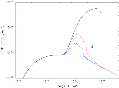
Figure 3: Modified energy loss for UHECR due to collisions. The figure shows the case $\alpha_{m}\neq 0$, for three different values of the weave scale $\mathcal{L}$. Curve 1: $\alpha_{m}=9\times 10^{-23}$ ($\mathcal{L}\simeq 8.6\times 10^{-18}$ eV^-1); curve 2: $\alpha_{m}=5\times 10^{-23}$ ($\mathcal{L}\simeq 1.2\times 10^{-17}$ eV^-1); curve 3: $\alpha_{m}=0$ (without modifications).

It can be seen therefore how the corrections can affect the main life time of protons propagating through the CMBR, allowing a strong improvement in the distances that protons can reach before loosing their characteristic energy (for energies greater than $1\times 10^{20}$ eV). The effects that the LQG corrections have on the propagation of UHECR are manifest through a decay of the energy loss in the range $E\sim 1\times 10^{20}$ eV. To understand this, recall relation (77) for the threshold condition of photo-pion production:

$$2\,\delta\alpha\,E_{\pi}^{2}+4E_{\pi}\omega\geqslant\frac{m_{\pi}^{2}(2m_{p}+m_{\pi})}{m_{p}+m_{\pi}}.$$ (144)

As we saw in section IV, the condition for a significant increase or decrease in the energy threshold can be calculated as $|\delta\alpha|\geqslant(2m_{p}+m_{\pi})(m_{p}+m_{\pi})/2E^{2}$. Therefore, for a given value of $\delta\alpha>0$, the energy at which the LIV effects start to take place is

$$E^{2}=\frac{1}{2\delta\alpha}(2m_{p}+m_{\pi})(m_{p}+m_{\pi}).$$ (145)

In the case $\alpha_{m}=9\times 10^{-23}$ (curve 1 of Fig.3), this energy is $E=1.1\times 10^{20}$ eV, while in the case $\alpha_{m}=5\times 10^{-23}$ (curve 2) this corresponds to $E=1.5\times 10^{20}$ eV. Beyond these energy scales, at about $E\sim 2\times 10^{20}$ eV, a sharp decay is observed in the behavior of the curve. This is due to the fact that the modified inelasticity $K$ will strongly constraint the energy-momentum phase space accessible to the final states depending on the initial energy $E$ that the primary proton carries (recall that now $K$ is a function of the energy $E$ of the incident proton and the energy $\epsilon$ of the CMBR photon).

We can also find the modified version of the UHECR spectrum for $\alpha_{m}\neq 0$. Fig.4 shows the AGASA observations and the predicted UHECR spectrum in the case $\alpha_{m}=1.5\times 10^{-22}$ ($\mathcal{L}\simeq 6.7\times 10^{-18}$ eV^-1) for three different maximum generation energies $E_{\mathrm{max}}$. These are, curve 1: $5\times 10^{20}$ eV; curve 2: $1\times 10^{21}$ eV; and curve 3: $3\times 10^{21}$ eV.

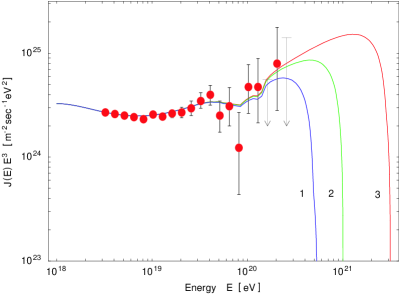
Figure 4: Modified UHECR spectrum and AGASA observations. The figure shows the modified spectrum $J(E)$ multiplied by $E^{3}$, for uniform distributed sources and without evolution, for the case $\alpha_{m}=1.5\times 10^{-22}$ ($\mathcal{L}\simeq 6.7\times 10^{-18}$ eV^-1). Three different maximum generation energies $E_{\mathrm{max}}$ are shown. These are, curve 1: $5\times 10^{20}$ eV; curve 2: $1\times 10^{21}$ eV; and curve 3: $3\times 10^{21}$ eV.

The Poisson probabilities of an excess in the five highest energy bins for the three curves are $P_{1}=3.6\times 10^{-4}$, $P_{2}=2.6\times 10^{-4}$ and $P_{3}=2.3\times 10^{-4}$. The Poisson $\chi^{2}$ for the eight highest energy bins are $\chi^{\,\,2}_{1}=10$, $\chi^{\,\,2}_{2}=10.9$ and $\chi^{\,\,2}_{3}=11.2$ respectively. The possibility of reconciling the data with finite maximum generation energies is significant given that conventional models require infinite maximum generation energies $E_{\mathrm{max}}$ for the best fit. For the lower part of the spectrum (under $E=4\times 10^{19}$ eV), the parameters under consideration leave the spectrum completely unaffected. This is due to the fact that in such a region the dominant reaction is the pair production, which has not being modified to obtain the spectrum. A more accurate study on this issue would require the computation of a modified inelasticity for the pair creation. Meanwhile, we must content ourself with the semiqualitative criteria given in section IV to rule out the parameters.

VI Conclusions

The scientific challenge that represents the search for new empirical backgrounds to test quantum gravity theories is at the embryonic stage. In this context, the possibility that ultra high energy cosmic rays could be experiencing quantum gravity effects places us in a very challenging situation which deserve attention. Nevertheless, the present stage of UHECR observations demands that we proceed with caution and patience.

We have seen how the kinematical analysis of the different reaction taking place in the propagation of ultra high energy protons can set strong bounds on the parameters to the theory. In comparison with our previous work, we have eliminated some previously open possibilities by the particular study of the pair creation $p+\gamma\rightarrow p+e^{+}+e^{-}$, in the energy region where this reaction dominates the proton’s interactions with the CMBR. In this way, the only possibility still open (for the corrective terms considered in the expansion (54) for the dispersion relations) and favored by the LQG scales, is the correction $\alpha$. If this is the case, a favored region for the scale length $\mathcal{L}$ estimated through the threshold analysis would be

$$2.6\times 10^{-18}\,\,\,\mathrm{eV}^{-1}\lesssim\mathcal{L}\lesssim 1.6\times 10^{-17}\,\,\,\mathrm{eV}^{-1}.$$

Similarly, the kinematical corrections can be studied in more detail when their effects are considered in the theoretical spectrum. In this regard, we have seen how to develop a modified version of the inelasticity for the photo-pion production, and its implications in the mean life time of a high energy proton as well as on the spectrum. To accomplish this last task we have only assumed a spontaneous Lorentz symmetry break up in the effective equations of motion, allowing the use of Lorentz transformations on the dispersion relations. Therefore, result (V.2) can be used in a more general context than the special case offered by the LQG framework.

Special mention must be made of a recent development AMU , where the dispersion relations for fermions and bosons are generalized to include the extra factor $\Upsilon$. It should be noted that this new factor always appears in the dispersion relations in the form $\left(l_{p}/\mathcal{L}\right)^{\Upsilon}$, such that the parameter $\alpha$ in our equation (44) gets an extra factor $\left(l_{p}/\mathcal{L}\right)^{\Upsilon-1}$. This freedom can be used to move the scale $\cal L$ down if needed, so that the cosmic ray momentum $p$ always satisfies the bound $p\,\mathcal{L}\leqslant 1$, without changing our prediction of the UHECR spectrum.

Future experimental developments like the Auger array, the Extreme Universe Space Observatory (EUSO) and Orbiting Wide-Angle Light Collectors (OWL) satellite detectors, will increase the precision and phenomenological description of UHECR. On the more theoretical side, progress in the direction of a full effective theory, with a systematic method to compute any correction with a known value for each coefficient, is one of the next steps in the “loop” quantization programme Thiemann2 ; Thiemann3 . Therefore, it is important to trace a phenomenological understanding of the possible effects that could arise as well as the constraints on LQG, in the high and low energy regimens (for other phenomenological studies of LQG effects, see for example SUV and Lambiase ).

References

- (1) D.J. Bird et al., Phys. Rev. Lett. 71, 3401 (1993).
- (2) M. Ave et al., Phys. Rev. Lett. 85, 2244 (2000).
- (3) K. Greisen, Phys. Rev. Lett. 16, 748 (1966).
- (4) G.T. Zatsepin and V.A. Kuzmin, Zh. Eksp. Teor. Fiz., Pisma Red. 4, 114 (1966).
- (5) F.W. Stecker, Phys. Rev. Lett. 21, 1016 (1968).
- (6) V. Berezinsky and S.I. Grigorieva, Astron. Atroph. 199, 1 (1988).
- (7) V. Berezinsky, A.Z. Gazizov and S.I. Grigorieva, hep-ph/0107306; hep-ph/0204357.
- (8) S.T. Scully and F.W. Stecker, Astropart. Phys. 16, 271 (2002).
- (9) T. Abu-Zayyad, astro-ph/0208243.
- (10) M. Takeda et al., Phys. Rev. Lett. 81, 1163 (1998). For an update see M. Takeda et al., Astrophys. J. 522, 225 (1999).
- (11) O.E. Kalashev, V.A. Kuzmin, D.V. Semikoz and I.L. Tkachev, astro-ph/0107130.
- (12) P.G. Tinyakov and I.I. Tkachev, astro-ph/0102476.
- (13) D.S. Gorbunov, P.G. Tinyakov, I.I. Tkachev and S.V. Troitsky, astro-ph/0204360.
- (14) T.W. Kephart and T.J. Weiler, Astropart. Phys. 4, 271 (1996).
- (15) D. Fargion, B. Mele, A. Salis, Astrophys. J. 517, 725 (1999).
- (16) T.J. Weiler, Astropart. Phys. 11, 303 (1999).
- (17) Z. Fodor, S.D. Katz, A. Ringwald, Phys. Rev. Lett. 88, 171101 (2002).
- (18) V. Berezinsky, M. Kachelriess and V. Vilenkin, Phys. Rev. Lett. 79, 4302 (1997).
- (19) T. Kifune, Astroph. J. Lett. 518, 21 (1999).
- (20) G. Amelino-Camelia and T. Piran, Phys. Lett. B 497, 265 (2001).
- (21) J. Ellis, N.E. Mavromatos and D.V. Nanopoulos, Phys. Rev. D 63, 124025 (2001).
- (22) G. Amelino-Camelia and T. Piran, Phys. Rev. D 64, 036005 (2001).
- (23) G. Amelino-Camelia, Phys. Lett. B 528, 181 (2002).
- (24) J. Alfaro and G. Palma, Phys. Rev. D 65, 103516 (2002).
- (25) G. Amelino-Camelia, Int. Journ. Mod. Phys. D 11, 35 (2002).
- (26) J. Magueijo and L. Smolin, Phys. Rev. Lett. 88, 190403 (2002).
- (27) J. Kowalski-Glikman, Mod. Phys. Lett. A 17, 1 (2002).
- (28) D. Colladay and V.A. Kostelecky, hep-ph/9703464.
- (29) D. Colladay and V.A. Kostelecky, hep-ph/9809521.
- (30) G. Amelino-Camelia, J. Ellis, N.E. Mavromatos, D.V. Nanopoulos, and S. Sarkar, Nature 393, 763 (1998).
- (31) O. Bertolami and C.S. Carvalho, Phys. Rev. D 61, 103002 (2000).
- (32) O. Bertolami, Nucl. Phys. Proc. Suppl. 88, 49 (2000).
- (33) S. Liberati, T.A. Jacobson, D. Mattingly, hep-ph/0110094.
- (34) T.J. Konopka and S.A. Major, New J. Phys. 4, 57.1 (2002).
- (35) J.M. Carmona, J.L. Cortés, J. Gamboa and F. Méndez, hep-th/0207158.
- (36) S. Liberati, T.A. Jacobson, D. Mattingly, hep-ph/0209264.
- (37) M. Gaul and C. Rovelli, Lect. Notes Phys. 541, 277 (2000).
- (38) Thiemann, gr-qc/0210094.
- (39) J. Alfaro, H.A. Morales-Técotl and L.F. Urrutia, Phys. Rev. Lett. 84, 2318 (2000).
- (40) J. Alfaro, H.A. Morales-Técotl and L.F. Urrutia, Phys. Rev. D 65, 103509 (2002).
- (41) J. Alfaro, H.A. Morales-Técotl and L.F. Urrutia, hep-th/0208192.
- (42) S. Coleman & S.L. Glashow, Phys. Rev. D 59, 116008 (1999).
- (43) K. Hagiwara et al., Phys. Rev. D 66, 010001 (2002).
- (44) D. De Marco, P. Blasi, A.V. Olinto, astro-ph/0301497.
- (45) R. Gambini and J. Pullin, Phys. Rev. D 59, 124021 (1999).
- (46) T. Thiemann, Class. Quant. Grav. 15, 1281 (1998).
- (47) F.W. Stecker and S.L. Glashow, Astropart.Phys. 16, 97 (2001).
- (48) J.M. Carmona and J.L. Cortés, Phys. Rev. D 65, 025006 (2002).
- (49) H. Sahlmann and T. Thiemann, gr-qc/0207030.
- (50) H. Sahlmann and T. Thiemann, gr-qc/0207031.
- (51) D. Sudarsky, L. Urrutia and H. Vucetich, gr-qc/0204027.
- (52) G. Lambiase, gr-qc/0301058.