Complex singularities of the critical potential in the large-$N$ limit

Abstract

We show with two numerical examples that the conventional expansion in powers of the field for the critical potential of 3-dimensional $O(N)$ models in the large-$N$ limit, does not converge for values of $\phi^{2}$ larger than some critical value. This can be explained by the existence of conjugated branch points in the complex $\phi^{2}$ plane. Padé approximants $[L+3/L]$ for the critical potential apparently converge at large $\phi^{2}$. This allows high-precision calculation of the fixed point in a more suitable set of coordinates. We argue that the singularities are generic and not an artifact of the large-$N$ limit. We show that ignoring these singularities may lead to inaccurate approximations.

I Introduction

Since the early days of the renormalization group (RG) method[1], 3-dimensional scalar models have been identified as an important laboratory to discuss the existence of non-trivial fixed points and the large cut-off (or small lattice spacing) limit of field theory models. In the case of $N$-components models with an $O(N)$ invariant Lagrangian, the RG transformation becomes particularly simple in the large-$N$ limit [2]. The construction of the effective potential for these models is discussed in Refs. [3, 4, 5]. Later, motivated by perturbative results indicating the existence of an UV stable tricritical fixed point for $N$ large enough[6], a new mechanism allowing spontaneous breakdown of scale invariance and dynamical mass generation was found in the large-$N$ limit[7]. In the following, we call this mechanism the “BMB mechanism”. It was argued[8] that the BMB mechanism is compatible with a zero vacuum energy and a better understanding of this question might suggest a solution to the cosmological constant problem. Spontaneous breaking of scale invariance is also discussed [9] with related methods in four-dimensional models of clear interest in the context of particle physics. However, doubts were cast[10] about the fact that the BMB mechanism is generic and it is commonly believed that it disappears at finite $N$.

In this article we report results which force us to reconsider the way we think about non-trivial fixed points. We usually think of the RG flows as taking place in a space of bare couplings or more generally in a space of functions. The necessity for this more general point of view appears quite clearly in exact renormalization group equations [11]. Unfortunately, it seems impossible to decide a-priori which space of functions should be considered to study the RG flows. It is clear from perturbation theory that near the Gaussian fixed point, low dimensional polynomial approximations of the local potential should be adequate. However, it is not clear that this kind of approximation should be valid far away from the Gaussian fixed point and in particular near non-trivial fixed points.

In the following, we concentrate on the non-trivial fixed point found numerically in the case $N=1$ by K. Wilson [1]. This fixed point is located on a hypersurface of second order phase transition which separates the symmetric phase from the broken symmetry phase. In the following we call this fixed point the Heisenberg fixed point (HFP for short) as in Ref. [10]. It should not be confused with the fixed point relevant for the BMB mechanism and which is not studied in detail here. The main result of the article is that the bare potential corresponding to the HFP has singularities in the complex plane and that ignoring these singularities may lead to inaccurate approximations. These claims are based on explicit calculations performed in the large-$N$ limit for two $O(N)$ invariant models reviewed in section II. These two models are: 1) a model with a $k^{2}$ kinetic term together with a sharp cut-off, the sharp cut-off model (SCM) for short; 2) Dyson’s hierarchical model (HM)[12, 13].

Before entering into technical details, three points should be clear. First, all the results presented here are based on the analysis of long numerical series and no attempt is made to give rigorous proofs. Second, in order to understand some of the statements made below, the reader should be aware that even though, at leading order in the large-$N$ approximation, the critical exponents take $N$-independent values, the same approximation provides finite $N$ approximate HFP which are $N$-dependent. A more precise formulation of this statement can be found in Sections II and VI. Third, we only work in 3 dimensions. The precise meaning of this statement for the hierarchical model is explained at the end of section II.

In section III, we review the basic equations [2, 10] defining the HFP for the SCM. We then show that the definition can be extended naturally for the HM. The correctness of this definition is verified later in the paper. In section IV, we present the methods used to calculate the critical potential expanded as a Taylor series in $\phi^{2}$. The coefficients of this expansion are called the critical couplings. The main conclusion that we can infer from our numerical results is that the Taylor series is inadequate for large values of $\phi^{2}$. First of all, one half of the critical couplings are negative. If we truncate the Taylor series at an order such that the coefficient of the highest order is negative, we obtain an ill-defined functional integral. In addition, the absolute value of the critical couplings grows exponentially with the order and the expansion has a finite radius of convergence. Consequently, the idea that the critical potential associated with the HFP can be approximated by polynomials should be reconsidered.

It is nevertheless possible to define the critical theory by using Padé approximants for the critical potential. In section V, we show that sequences of approximants converge toward the expected function in a way very reminiscent of the case of the anharmonic oscillator were the convergence can be proven rigorously [14]. In addition, the zeroes and the poles of these approximants are located far away from the real positive axis and follow patterns that strongly suggest the existence of two complex conjugated branch points.

The complex singularities of the critical potential should not be interpreted as a failure of the RG approach but rather as an artifact of the system of coordinates used. In section VI, we present consistent arguments showing that in a different system of coordinates [15, 16], the function associated with the HFP is free of singularities. In this system of coordinates, finite dimensional truncation is a meaningful procedure which, in the case of the HM, allows comparison with independent numerical calculations at finite $N$. An example of such a calculation is presented in the case $N=5$.

In section VII, we discuss the errors associated with two approximate procedures that can be used to deal with the singularities. The first procedure which is justified in the context of perturbation theory and does not require an understanding of the singularities, consists in truncating the potential at order $(\phi^{2})^{3}$. The second procedure consists in restricting the range of integration of $\phi^{2}$ to the radius of convergence of the critical potential. If the range of integration is large enough, this second procedure generates small errors [17]. As far as the calculation of the HFP in the system of coordinates of Section VI is concerned, both procedures have a low accuracy for both models considered. In the conclusions, we explain why we believe that the singularities persist at finite $N$ and we discuss implications of the existence of these singularities for other problems.

II Models

We consider lattice models defined by the partition function

$$Z(\vec{J})=\prod_{x}\int d^{N}\phi_{x}{\rm e}^{-S+\sum_{x}\vec{J}_{x}\vec{\phi}_{x}}\ ,$$ (1)

with

$$S=-{1\over 2}\sum_{xy}\vec{\phi}_{x}\Delta_{xy}\vec{\phi}_{y}+\sum_{x}V_{o}(\phi^{2}_{x})\ .$$ (2)

We use the notation $\phi^{2}_{x}\equiv\vec{\phi}_{x}.\vec{\phi}_{x}$ and $\Delta_{xy}$ is a symmetric matrix with negative eigenvalues, such as discrete versions of the Laplacian. For the simplicity of the presentation, we will assume that $\sum_{x}\Delta_{xy}=0$. If it is not the case, one can always subtract the zero mode from $\Delta$ and compensate it with a new term in $V$.

Defining the rescaled potential

$$V_{0}(X)=NU_{0}({X\over N})\ ,$$ (3)

and performing a Legendre transform from the source $\vec{J}$ to the external classical field $\vec{\phi}_{c}$, one can show that in the large $N$ limit[10] that $M^{2}\equiv 2\partial V_{eff}/\partial\phi^{2}_{c}$ obeys the self-consistent equation

$$2U_{0}^{\prime}(\phi_{c}^{2}+f_{\Delta}(M^{2}))=M^{2}\ ,$$ (4)

where $f_{\Delta}(M^{2})$ is the one-loop integral corresponding to the quadratic form $\Delta$ and a mass term $M^{2}$. The prime denotes the derivative with respect to the $O(N)$ invariant argument. The explicit form of $f$ for the two models discussed in the following are given in Eqs. (7-8). Precise definitions of $\phi^{2}_{c}$ and the effective potential $V_{eff}$ are given in [10].

Up to now, all the quantities introduced are dimensionless. They can be interpreted as dimensionful quantities expressed in cut-off units. Let us consider two models, the first one with a rescaled potential $U_{0}$, a UV cutoff $\Lambda$ and a quadratic form $\Delta$ and a second model with a rescaled potential $U_{0,S}$, a UV cutoff $\Lambda/S$ and a quadratic form $\Delta_{S}$. For $D=3$ and in the large-$N$ limit, the two models have the same dimensionful zero-momentum Green’s functions provided that:

$$U {}^{\prime}_{0,S}(\phi^{2})=$$ (5)

$$S {}^{2}U_{0}^{\prime}\biggl{(}\bigl{(}\phi^{2}-f_{\Delta_{S}}(2U^{\prime}_{0,S}(\phi^{2})\bigr{)}/S+f_{\Delta}\bigl{(}(2/S^{2})U^{\prime}_{0,S}(\phi^{2})\bigr{)}\biggr{)}$$ (6)

In two special cases, the dimensionless expression for the one-loop diagram is independent of the cut-off. In other words, $f_{\Delta}=f_{\Delta_{S}}\equiv f$ and the fixed point equation becomes very simple [2, 10].

We now discuss the two models where this simplification occurs. In the SCM, $\Delta$ becomes $k^{2}$ in the momentum representation (Fourier modes). The momentum cutoff is sharp: $k^{2}\leq 1$ (in cut-off units). This is why we call this model the sharp cutoff model. The non-renormalization of the kinetic term is justified in the large-$N$ limit [10]. For this model,

$$f_{SCM}(z)=\int_{|k|\leq 1}{{d^{3}k}\over{(2\pi)^{3}}}{1\over{k^{2}+z}}\ .$$ (7)

By construction [13], the kinetic term of Dyson’s hierarchical model (HM) is not renormalized and we have

$$f_{HM}(z)=\sum_{n=0}^{\infty}{{2^{-n-1}}\over{b(c/2)^{n}+z}}\ ,$$ (8)

with $c=2^{1-2/D}$ and $b$=${\beta c\over{2-c}}$. The inverse temperature $\beta$ and the parameter $c$ appear in the hamiltonian of the HM in a way that is explained in section II of Ref. [18]. The parameter $c$ is related to the dimension $D$ by considering the scaling of a massless Gaussian field. In the following we will consider the case $c=2^{1/3}$ ($D=3$) exclusively. In addition, $\beta$ will be set to 1 as in other fixed point calculations [18]. Different values of $\beta$ can be introduced by a trivial rescaling. Note also that the cutoff cannot be changed continuously for the HM, because the invariance of $f$ is only valid when we integrate the degrees of freedom of a the largest momentum shell (corresponding to the hierarchically nested blocks in configuration space) all at the same time. For the HM, the density of sites is reduced by a factor 2 at each RG transformation. The linear dimension (“lattice spacing”) is thus increased by by a factor $2^{1/D}$ and the cutoff decreased by the same factor. Consequently, for the HM, Eq. (5) should be understood only with $S=2^{q/D}=2^{q/3}$ and $q$ integer.

III The HFP

In this section, we review the construction of the HFP for the SCM, and we show that the construction can be extended in a natural (but non-trivial) way for the HM. The first step consists in finding all the fixed points of the RG Eq. (5). Following Refs. [2, 10], we introduce the inverse function:

$$F(2U^{\prime}_{0}(\phi^{2}))=\phi^{2}\ ,$$ (9)

and the function $H(z)\equiv F(z)-f(z)$ , where the one-loop function $f$ has been defined in the previous section for the two models considered. With these notations, the fixed point equation corresponding to Eq. (5) is simply

$$H(z)=SH(z/S^{2})\ .$$ (10)

For the SCM, $S$ is allowed to vary continuously in Eq. (10) and the general solution is

$$F(z)=f_{SCM}(z)+Kz^{1/2}\ .$$ (11)

For the HM, $S$ can only be an integer power of $2^{1/3}$ and the general solution has an infinite number of free parameters:

$$F(z)=f_{HM}(z)+\sum_{q}K_{q}z^{1/2+iq\omega}\ ,$$ (12)

with

$$\omega\equiv{3\pi\over{{\rm ln}2}}\simeq 13.6\ ,$$ (13)

and $q$ runs over positive and negative integers. The only restriction on the constants $K$ and $K_{q}$ is that $F$ should have a well defined inverse which is real when $F(=\phi^{2})$ is real and positive.

It is clear from Eqs. (7) and (8) that for both models $f(z)$ has singularities along the negative real axis and that, in general, $F(z)$ cannot be defined for $z$ real and negative. This imposes restrictions on the choice of the constants $K$ and $K_{q}$. For instance, in the case of the SCM, when $K$ takes a large positive value, it is impossible to reach small values of $F=\phi^{2}$ when $z\geq 0$ and the fixed point has no obvious physical interpretation. However, there is a special positive value of $K$ for which the singularity of $f_{SCM}$ is exactly canceled and an analytic continuation for $z<0$ is possible. Its exact value can be calculated [10] by decomposing $f_{SCM}$ into a regular part $f_{SCM,reg.}$ and a singular part $f_{SCM,sing.}$. Using elementary trigonometric identities, one finds

$$f_{SCM,reg.}(z)={1\over{2\pi^{2}}}(1+z^{1/2}{\rm Arctan}(z^{1/2}))\ ,$$ (14)

and

$$f_{SCM,sing.}(z)=-{1\over{4\pi}}z^{1/2}\ .$$ (15)

Consequently, if we choose $K={1\over{4\pi}}$, $F$ reduces to $f_{SCM,reg.}$.

A more detailed analysis [10], shows that this value of $K$ is the only positive value of $K$ for which $U^{\prime}$ can be defined for any real positive $\phi^{2}$. On the other hand, for negative $K$, one obtains a line of fixed points ending (for $K=0$) at the fixed point relevant for the BMB mechanism. Given the isolation of the fixed point with $K={1\over{4\pi}}$, it is easy to identify it with the HFP. We denote the corresponding inverse function by $F^{\star}_{SCM}(z)=f_{SCM,reg.}(z)$. As promised this function is analytical in a neighborhood of the origin and has a Taylor expansion:

$$F^{\star}_{SCM}(z)={1\over{2\pi^{2}}}(1+z-{z^{2}\over 3}+{z^{3}\over 5}+\dots)$$ (16)

This expansion has a radius of convergence equal to 1 due to a logarithmic singularity at $z=-1$. However, as we will see in section IV, this expansion allows us to construct an inverse power series and $U_{0}$.

In the case of the HM, the decomposition into a regular and singular part is more tedious. Fortunately, this problem is a particular case of a problem solved in section 5 of Ref. [19] where Eq. (5.6) with $A=c^{2}$, $B=c^{-1}$ and $f(z)=G(z/b)$ yields

$$f_{HM,sing.}(z)=-{\omega\over{4b}}\sum_{q}{\bigl{(}{z/b}\bigr{)}^{1/2+iq\omega}\over{\rm sin}(\pi(1/2+iq\omega))}\ ,$$ (17)

with $b$ and $c$ defined in section II.

If we compare this expression with the general solution of the fixed point equation (12), we see that in both expressions, the power $z^{1/2+iq\omega}$ appears for all positive and negative integer values of $q$. There exists a unique choice of the $K_{q}$ in Eq. (12) which cancels exactly the singular part of $f_{HM}$. We call the corresponding fixed point the HFP of the HM. The numerical closeness with the finite $N$ HFP discussed in section VI confirms the validity of this analogic definition. We call the corresponding inverse function $F_{HM}^{\star}$. Using Eq. (5.5) of Ref. [19], we find

$$F_{HM}^{\star}(z)=f_{HM,reg.}={1\over{2b}}\sum_{l=0}^{\infty}\biggl{(}{-z\over b}\biggr{)}^{l}{1\over{1-c^{2l-1}}}\ .$$ (18)

This expansion has a radius of convergence $bc^{2}=2.7024\dots$ for the choice of parameters used here.

It is possible to check the accuracy of the expansion given in Eq. (18) by using the identity $F_{HM}^{\star}(z)=f_{HM}(z)-f_{HM,sing.}$. Note that the two terms of the r.h.s. cannot be defined separately on the negative real axis. On the real positive axis, $f_{HM,sing.}$ is dominated by the $q=0$ term. Numerically,

$$K_{0}={3\pi\over{4b^{3/2}{\rm ln}2}}=1.530339\dots.$$ (19)

The terms with $q=\pm 1$ produce log-periodic oscillations of amplitude $1.7\times 10^{-18}$. The terms with larger $|q|$ have a much smaller amplitude. These findings are consistent with the log-periodic oscillations found numerically in HT expansions [20, 19]. The oscillatory terms are very small along the positive real axis. However, in the complex plane, if we write $z=r{\rm e}^{i\theta}$, the amplitude is multiplied by ${\rm e}^{-q\omega\theta}$ which compensates the suppression of the denominators in Eq. (17), if $\theta\rightarrow+\pi(-\pi)$ when $q<0$ ($q>0$). In conclusion, along the real positive axis, we can use the approximation

$$F_{HM}^{\star}(z)\simeq f_{HM}(z)+K_{0}z^{1/2}\ ,$$ (20)

with an accuracy of 18 significant digits, but this approximation is certainly not valid near the negative real axis.

IV Calculation of the critical potential $U_{0}^{\star}$

In the previous section, we have provided power series for the inverse function $F(z)$ corresponding to the HFP of the SCM and the HM. We can use these series to define $F(z)$ on the negative real axis. In both cases, as we move toward more negative values of $z$, $F$ becomes zero within the radius of convergence of the expansion. The situation is illustrated in Fig. 1 for the HM.

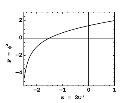
FIG. 1.: $F_{HM}^{\star}(z)$ versus $z$

Numerically, we have $F_{HM}^{\star}(-1.5107\dots)=0$ and $F_{SCM}^{\star}(-0.6948\dots)=0$. We then reexpand the series about that value of $z$ (which corresponds to $F=\phi^{2}=0$) and invert it. The resulting series is an expansion of $2U_{0}^{\star}$’ in $\phi^{2}$. After integration, and up to an arbitrary constant $u_{0}$, we obtain a Taylor series for the critical potential $U_{0}^{\star}$ corresponding to the HFP. We denote the expansion as

$$U_{0}^{\star}(\phi^{2})=\sum_{n=0}^{\infty}u_{n}(\phi^{2})^{n}\ .$$ (21)

The precise determination of the zero of $F$ is obtained by Newton’s method with a large order polynomial expansion. This expansion is then reexpanded about the zero and the large order coefficients in the original expansion have an effect on the low order coefficients of the reexpanded series. We have checked that the order was sufficiently large to stabilize the results presented hereafter.

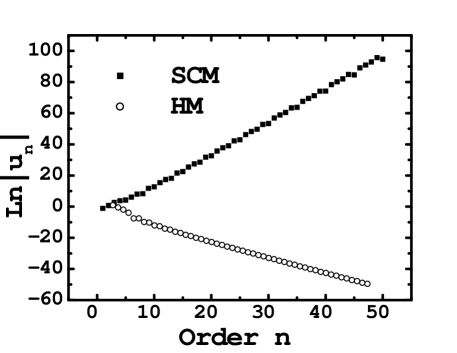
FIG. 2.: Natural Logarithm of the absolute value of the coefficients $u_{n}$ of the critical potential $U_{0}^{\star}$ defined in Eq. (21) for the SCM (filled squares) and the HM (empty circles).

The absolute values of the first 50 coefficients of both models are shown in Fig. 2. In both cases, it appears clearly that the absolute value grows at an exponential rate. Linear fits of the right part of Fig. 2 suggest a radius of convergence of order 0.11 for the SCM and 2.5 for the HM. The signs of both series follow the periodic pattern: + - - + + - + + - - for the SCM and + + - - for the HM. This suggests singularities in the complex plane at an angle ${k\pi\over 5}$ with respect to the positive real axis ($k=$ 1, 3, 7, 9) for the SCM and along the imaginary axis for the HM. This analysis is confirmed by an analysis of the poles of Padé approximants presented in the next section.

V Padé approximants of $U_{0}^{\star}$

At this point, our series expansion of the critical potential does not allows us to define the critical theory as a functional integral. As $\phi^{2}$ exceeds the critical values estimated in the previous section, the power series is unable to reproduce the expected function $U_{0}^{\star}$. The situation is illustrated in Fig. 3 for the HM.

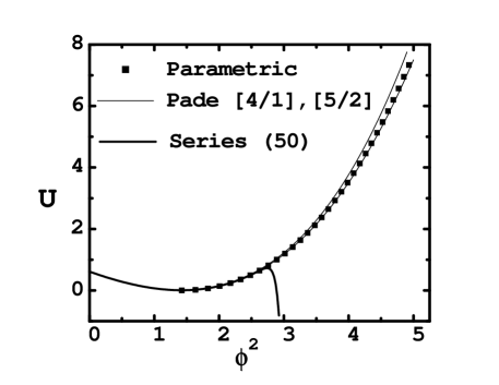
FIG. 3.: $U_{0}^{\star}(\phi^{2})$ for the HM with a parametric plot (filled squares), the series truncated at order 50 (thick solid line) and Padé approximants [4/1] (thin line slightly above the squares) and [5/2] (thin line closer to the squares). The constant has been fixed in such a way that the value at the minimum is zero.

The numerical values of $U_{0}^{\star}$ in Fig. 3 have been calculated using a parametric representation (with $z$ as the parameter). We have calculated pairs of values

$$\left(F^{\star}(z),{1\over 2}\bigl{(}zF^{\star}(z)-\int_{0}^{z}dz^{\prime}F^{\star}(z^{\prime})\bigr{)}\right)\ ,$$ (22)

for various real positive values of $z$. A simple graphical analysis performed by representing $U_{0}^{\star}$ as a surface on Fig. 1 shows that each pair of values in in Eq. (22) corresponds to a pair $(\phi^{2},U_{0}^{\star}(\phi^{2}))$ with the arbitrary constant in $U_{0}^{\star}$ fixed in such a way that $U_{0}^{\star}$ vanishes at its minimum. We have calculated $F^{\star}$ by using the independent but approximate Eq. (20). As explained in section III, the approximate expression is only valid for $z$ real and positive and should give 18 correct significant digits. In Fig. 3, we have used the values $z=2U^{\prime}_{0}=0,\ 0.25,0.5,\dots$. This is why the filled squares only appear when the derivative of $U_{0}^{\star}$ is positive. Unlike Eq. (18) which has a radius of convergence 1, the approximate expression Eq. (20) remains valid for large positive values of $z$. It is thus possible to check if Padé approximants can be used to represent the critical potential beyond the radius of convergence of its Taylor expansion. Fig. 3 shows that low order approximants are close to the parametric curve. As the order increases, the curves coalesce with the parametric curve and a more refined description is necessary.

In Fig. 4, we give the accuracy reached by various approximants for the HM with a broad range of $\phi^{2}$ (more than 4 times the radius of convergence). As the order of the approximants increase the accuracy increases but at a rate which is slower for larger values of $\phi^{2}$. The figure is very similar to sequences of Padé approximants obtained for the ground state of the anharmonic oscillator (see Fig. 1 of Ref. [17]), where the convergence can be proven rigorously [14]. Note that the slow convergence at large $\phi^{2}$ is not a serious problem, since the contributions for large $\phi^{2}$ are exponentially suppressed in the functional integral. The choice of $[L+3/L]$ approximants is discussed in more detail below. Up to now, we only discussed the HM. Following the same procedure for the SCM, we obtain very similar figures (with a different $\phi^{2}$ scale) which we have not displayed.

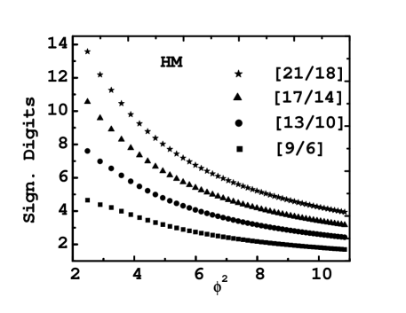
FIG. 4.: Number of correct significant digits obtained with Padé approximants [9/6], [13/10], [17/14] and [21/18] for various values of $\phi^{2}$ for the HM.

The singularities of $U_{0}^{\star}$ in the complex $\phi^{2}$ plane can be inferred from the location of the zeroes and poles of the Padé approximants. As $L$ becomes large, regular patterns appear. Examples are shown in Fig. 5 for the SCM and Fig. 6 for the HM. In both cases, the zeroes and poles approximately alternate along two lines ending where singularities were expected from the analysis of coefficients in Section IV. This pattern suggests [21] the existence of two complex conjugated branch points at the end of these lines.

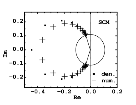
FIG. 5.: Real and imaginary parts of the roots of the denominator (filled squares) and numerator (crosses) of a [26/23] Padé approximant for the SCM The solid circle has a radius 0.11 and the two solid lines make angles $\pm{3\pi\over 5}$ with respect to the positive real axis.

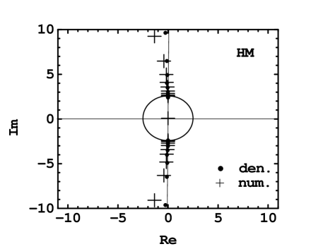
FIG. 6.: Real and imaginary parts of the roots of the denominator (filled circles) and numerator (crosses) of a [26/23] Padé approximant for the HM. The solid circle has a radius 2.5. Two roots farther away on the imaginary axis and one root farther away near the negative real axis are not displayed.

The choice of $[L+3/L]$ approximants is easily justified for the SCM. At large $|z|$, $f_{SCM}(z)\propto 1/z$ and and $F^{\star}_{SCM}(z)\simeq{1\over{4\pi}}z^{1/2}$. For large $|\phi^{2}|$, $U_{0}^{\star}$’$\simeq 8\pi^{2}(\phi^{2})^{2}$ and $U_{0}^{\star}\simeq{8\pi^{2}\over{3}}(\phi^{2})^{3}$. Consequently a $[L+3/L]$ approximant should have the correct asymptotic behavior. More precisely, if $a_{L+3}$ and $b_{L}$ are the leading coefficients of the numerator and denominator of a Padé $[L+3/L]$ respectively, we expect that when $L$ is large

$${a_{L+3}\over b_{L}}\rightarrow{8\pi^{2}\over 3}$$ (23)

Defining a quantity

$$E_{L}\equiv 1-{{3a_{L+3}}\over{8\pi^{2}b_{L}}}\ ,$$ (24)

that measures the departure from the expected asymptotic behavior, we see from Fig. 7 that as $L$ increases, the discrepancy diminishes exponentially.

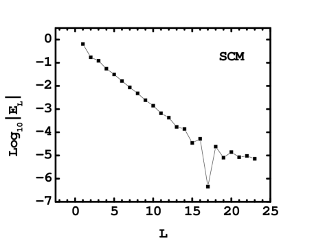
FIG. 7.: Log$|E_{L}|$ versus $L$.

In the case of the HM, the situation is more intricate. From Eq. (20), we may be tempted to conclude that the two cases are similar. Unfortunately, Eq. (20) is a real equation not a complex one. In the complex plane, the terms with $q\neq 0$ become important near the negative real axis and no simple simple limit as in Eq. (23) applies. However, if we need $U_{0}^{\star}$ only along the real positive axis, Fig. 4 justifies the use of the $[L+3/L]$ sequence of approximants.

VI The HFP in a convenient set of coordinates

As explained in the introduction we can think that the RG flows move in a space of functions. The system of coordinates for this space can be chosen in a way which is convenient to make approximations. A particularly convenient system of coordinates for the HM consists in considering the Fourier transform of the local measure of integration [15, 16]. In this system of coordinates and at leading order in the $1/N$ expansion, the HFP for a given $N$ reads:

$$R^{\star}(\vec{k})\propto\int d^{N}\phi{\rm e}^{-{b\over 2}\phi^{2}-NU_{0}^{\star}(\phi^{2}/N)+i\vec{k}.\vec{\phi}}\ .$$ (25)

The quadratic term proportional to $b$ is due to the fact that the quadratic form $\Delta$ for the HM has a zero mode. We then Taylor expand

$$R^{\star}(\vec{k})=1+\sum_{n=1}^{\infty}a_{n}(k^{2})^{n}\ ,$$ (26)

and consider the $a_{n}$ as the our new set of coordinates. The advantage of this representation is that it is possible to make very accurate calculations by using polynomial approximations [15, 16, 18] of the infinite sum in Eq. (26). In this section and the next section, we discuss the details of the calculations for the HM. The case of the SCM shares many similarities with the HM and is discussed briefly at the end of each section.

We have performed a numerical calculation of the $a_{n}$ of the HM using Eq. (25) in the particular case $N=5$. The study of the ratios of successive coefficients displayed in Fig. 8 indicates that the $|a_{n}|$ decay faster than $1/n!$ and that $R^{\star}(\vec{k})$ is analytical over the entire complex $k^{2}$ plane in contrast to $U_{0}^{\star}(\phi^{2})$ which has a finite radius of convergence in the complex $\phi^{2}$ plane.

The good convergence of $R^{\star}(\vec{k})$ can be explained by an approximate calculation. The $\phi$ integral that is performed in the calculation of the $a_{n}$ has a positive integrand with a peak moving to larger values of $|\phi|$ when $n$ increases. For sufficiently large values of $n$, we can replace $U_{0}^{\star}$ by its asymptotic behavior on the positive real $\phi^{2}$ axis which can be derived from the approximate Eq. (20) for the HM:

$$R^{\star}(\vec{k})\sim\int d^{N}\phi{\rm e}^{-(1/(6N^{2}K_{0}^{2}))(\phi^{2})^{3}+i\vec{k}.\vec{\phi}}\ .$$ (27)

With this approximation, the $a_{n}$ can be expressed exactly in terms of gamma functions and a simple calculation yields

$$-{a_{n}\over{a_{n-1}}}\simeq{{(6N^{2}K_{0}^{2})^{1/3}\Gamma((N+2n)/6)}\over{4n(n-1+N/2)\Gamma((N+2(n-1))/6)}}\ .$$ (28)

Note that there are no free parameters in this formula. Fig. 8 shows that Eq. (28) is a very good approximation of the ratios obtained numerically from Eq. (25).

We have also calculated the $a_{n}$ corresponding to the HFP for $N=5$ using the numerical method developed in the case $N=1$ in Ref. [18] and which can be extended easily for arbitrary $N$. In brief, it consists of finding the stable manifold by fine tuning the temperature and then iterating the RG transformation in order to get rid of the irrelevant directions. This procedure is very accurate and completely independent of the approximations made in this article. Remarkably, we found that even though $N=5$ is not a large number, the first coefficients obtained in the leading order in the $1/N$ approximation coincide with about two significant digits with the accurate values found numerically with $N=5$. As the order increases, the accuracy degrades slowly. This is explained in more detail below. However, the ratios of successive coefficients still follows closely the asymptotic prediction obtained from Eq. (28). This strongly suggests that the $(\phi^{2})^{3}$ asymptotic behavior of the critical potential persists at finite $N$.

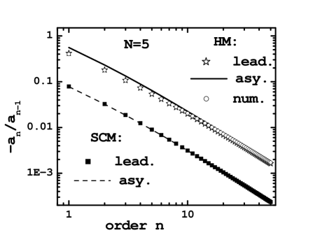
FIG. 8.: Ratios of successive coefficients for the HM, using the leading order Eq. (25) (stars), the asymptotic formula Eq. (28) (continuous line) and the numerical fixed point (empty circles). Same results for the SCM: leading order (filled squares) and asymptotic (dashed line). In all cases, $N=5$.

Except for the comparison with independent numerical calculations at finite $N$, the same calculations can be performed for the SCM with minor changes ($b\rightarrow 0$ and $K_{0}\rightarrow K$). The results are also shown in Fig. 8 where one can see that the agreement with the asymptotic formula is very good even at low order.

VII Discussion of alternate procedures

In section V, we have shown that the Padé approximants provide accurate values of $U_{0}^{\star}$ far beyond its radius of convergence. In order to estimate the error on the new coordinates $a_{n}$ due to the use of approximants for $U_{0}^{\star}$, we can vary the range of integration and change the approximants. For instance the values of $a_{n}$ of the HM used in Fig. 8 have been calculated using a range of integration $|\phi|<20$ and a [26/23] Padé approximant. For the values of $n$ considered here, changing the range of integration has effects smaller than the errors due to numerical integration (which has an accuracy of about 11 significant digits in our calculation) provided that we include values up to $|\phi|\simeq 4.9$. Restricting the range of integration to smaller values produces sizable effects. As an example, the small effects due a restriction to $|\phi|<4.4$ are shown in Fig. 9. Similarly, the values of $a_{n}$ are not very sensitive to small changes in the Padé approximants. Sizable effects are obtained by changing the order of the numerator and denominator by approximately 10. For instance, the effects of using a [14/11] approximant are shown in Fig. 9.

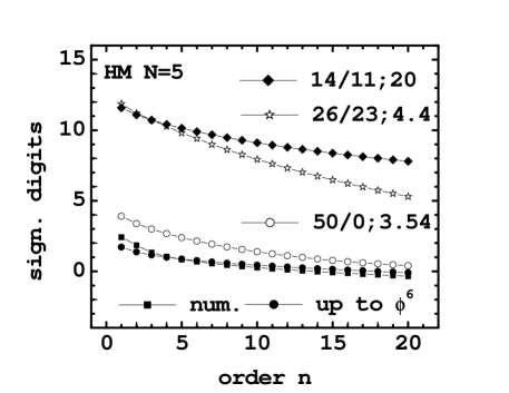
FIG. 9.: Number of significant digits common with our best estimate for the $a_{n}$ obtained for the HM from Eq. (25) with $n$ (the order) going from 1 to 20. The alternate procedure are the truncation at order $(\phi^{2})^{3}$ (filled circles), the $N=5$ accurate numerical result (filled square), no Padé approximants but a truncation of the range of integration close to the radius of convergence (empty circles), a restriction of the range of integration for $\phi<4.4$ (stars), and a [14/11] Padé (diamonds).

Having demonstrated that we can calculate the first 20 coefficients $a_{n}$, at leading order in the $1/N$ expansion, with at least 10 significant digits, we can now discuss the errors associated with other procedures mentioned in the introduction. The first procedure consists in truncating $U_{0}^{\star}$ keeping only the terms up to order $(\phi^{2})^{3}$. This is procedure inspired by perturbation theory amounts to keep only the relevant and marginal directions near the Gaussian fixed point. From Fig. 9, we see that this procedure generates errors which are of the same order as the errors due to the use of the leading $1/N$ approximation. Consequently, this procedure is quite unsuitable to study the correction to this approximation. Slightly better results are obtained by keeping as many terms as possible in the expansion (up to 50 in our calculation) but restricting the range of integration in such way that we stay within the radius of convergence. Given the rescaling of Eq. (3) this means that for $N=5$, we need to restrict the integration to $|\phi|<\sqrt{5\times 2.5}\simeq 3.54$ which is substantially smaller than the acceptable field cutoff 4.9 mentioned above. As one can see from Fig. 9, this creates errors which are between one and two orders of magnitude smaller than the $1/N$ corrections. This is better but it compares poorly with what can reached with Padé approximants.

Again, except for the comparison with independent numerical calculations at finite $N$, the same calculations can be performed for the SCM with minor changes. Results very similar to those shown in Fig. 9 for the HM can be produced. Since it contains essentially the same information, it has not been displayed. It should however be noted that the number of significant digits obtained with the two alternate procedures are lower than in the case of the HM. In the case of the truncation of the range of integration, we need to restrict to $|\phi|<\sqrt{5\times 0.11}\simeq 0.74$ while a range of about 2 is required in order to obtain an accuracy consistent with the method of numerical integration.

VIII Conclusions

We have shown in two differents models where the critical potential can be calculated at leading order in the $1/N$ expansion that these potentials have finite radii of convergence due to singularities in the complex plane. Do such a results persist at finite $N$? In the case of the HM, the behavior of the ratios at finite $N$ shown in Fig. 8 strongly suggests that at large real positive $\phi^{2}$, the critical potential still grows like $(\phi^{2})^{3}$. Can an infinite sum converging over the entire complex plane have this kind of behavior? This is certainly not impossible (e.g., $(\phi^{2})^{3}+{\rm e}^{-\phi^{2}}$), however it requires cancellations that we judge unlikely to happen. Consequently, we conjecture that the singularities observed are generic rather than being an artifact of the large-$N$ limit.

We have observed that in a system of coordinates where the HFP can be approximated by polynomials, the procedure which consists in considering bare potential truncated at order $(\phi^{2})^{3}$ describes the HFP with a low accuracy. We are planning to investigate if similar problems appear near tricritical fixed points. In particular, reconsidering the RG flows in a larger space of bare parameters may affect the generic dimension of the intersections of hypersurface of various codimensions and help us finding a more general realization of spontaneous breaking of scale invariance with a dynamical generation of mass.

Our results have qualitative similarities common with those of Refs. [22]: we found some “pathologies” which force us to look at the RG transformations in a more open-minded way. We are planning [23] to compare in more detail, the leading order results presented here with finite $N$ results, as suggested in Ref. [24] for the local potential approximation. Another issue regarding the $O(N)$ models and which would deserve a more detailed investigation is the question of first order phase transitions[25, 26].

REFERENCES

- [1] K. Wilson, Phys. Rev. D 6, 419 (1972).
- [2] E. Ma, Rev. Mod. Phys. 45, 589 (1973).
- [3] S. Coleman, R. Jackiw and H. Politzer, Phys. Rev. D 10 2491 (1974).
- [4] P. Townsend, Phys. Rev. D 14 1715 (1976).
- [5] T. Appelquist and U. Heinz, Phys. Rev. D 24 2169 (1981).
- [6] R. Pisarski, Phys. Rev. Lett. 48, 574 (1982).
- [7] W. Bardeen, M. Moshe and M. Bander, Phys. Rev. Lett. 52, 1188 (1984).
- [8] D. Amit and E. Rabinovici, Nucl. Phys. B 257, 371 (1985).
- [9] W. Bardeen, C. Leung and S. Love, Phys. Rev. Lett. 56, 1230 (1986); W. Bardeen and M. Moshe, Phys. Rev. D 34, 1229 (1986); W. Bardeen, Fermilab preprint CONF-88/149-T (1988).
- [10] F. David, D. Kessler and H. Neuberger, Phys. Rev. Lett. 53, 2071 (1984); F. David, D. Kessler and H. Neuberger, Nucl. Phys. B 257, 695 (1985).
- [11] There is a large literature on this question. Extensive lists of references can be found in two recent reviews: C. Bagnuls and C. Bervillier, Phys. Reports 348, 91 (2001); J. Berges, N. Tetradis and C. Wetterich, Phys. Reports 362, 223 (2002).
- [12] F. Dyson, Comm. Math. Phys. 12, 91 (1969).
- [13] G. Baker, Phys. Rev. B5, 2622 (1972).
- [14] J. Loeffel, A. Martin, B. Simon, and A. Wightman, Phys. Lett. B 30, 656 (1969).
- [15] H. Koch and P. Wittwer, Comm. Math. Phys. 164, 627 (1994).
- [16] J. Godina, Y. Meurice, and M. Oktay, Phys. Rev. D 57, 6326 (1998).
- [17] Y. Meurice, Phys. Rev. Lett. 88, 141601 (2002).
- [18] J. Godina, Y. Meurice, and M. Oktay, Phys. Rev. D 57, R6581 (1998); J. Godina, Y. Meurice, and M. Oktay, Phys. Rev. D 59, 096002 (1999).
- [19] Y. Meurice, G. Ordaz and S. Niermann, J. Stat. Phys. 87, 363 (1997).
- [20] Y. Meurice, G. Ordaz and V. G. J. Rodgers, Phys. Rev. Lett. 75, 4555 (1995).
- [21] G. Baker and P. Graves-Morris, Padé Approximants (Cambridge University Press, Cambridge, 1996).
- [22] A. van Enter, R. Fernandez and A. Sokal, J. Stat. Phys. 72, 879 (1993); A. van Enter and R. Fernandez, Phys. Rev. E 59, 5165 (1999).
- [23] J. J. Godina, L. Li, Y. Meurice and B. Oktay, work in progress.
- [24] J. Comellas and A. Travesset, Nucl. Phys. B 498, 539 (1997).
- [25] P. Hasenfratz and A. Hasenfratz, Nucl. Phys. B 295, 1 (1988).
- [26] A. van Enter and S. Shlosman, cond-mat/0205455.