hep-th/0208178
AEI 2002-061

Correlation functions in perturbative $\mathcal{N}=4$ supersymmetric Yang-Mills theory are examined in the Berenstein-Maldacena-Nastase (BMN) limit. We demonstrate that non-extremal four-point functions of chiral primary fields are ill-defined in that limit. This lends support to the assertion that only gauge theoretic two-point functions should be compared to pp-wave strings. We further refine the analysis of the recently discovered non-planar corrections to the planar BMN limit. In particular, a full resolution to the genus one operator mixing problem is presented, leading to modifications in the map between BMN operators and string states. We give a perturbative construction of the correct operators and we identify their anomalous dimensions. We also distinguish symmetric, anti-symmetric and singlet operators and find, interestingly, the same torus anomalous dimension for all three. Finally, it is discussed how operator mixing effects modify three point functions at the classical level and, at one loop, allow us to recover conformal invariance.

1 Introduction and overview

Recently, a very interesting proposal for taking a novel kind of large $N$ limit in a gauge theory was made [1]. The proposal is to consider correlation functions of gauge invariant operators with a large SO(2) charge $J$ in $\mathcal{N}=4$ Super Yang-Mills theory, where SO(2) is a subgroup of the full SO(6) R-symmetry group of this gauge theory. This Berenstein-Maldacena-Nastase (BMN) limit is then

$$N\to\infty~{}~{}{\rm and}~{}~{}J\to\infty~{}~{}{\rm with}~{}~{}\frac{J^{2}}{N}~{}~{}{\rm fixed},~{}~{}g_{\scriptscriptstyle\mathrm{YM}}~{}~{}{\rm fixed}$$ (1.1)

where $N$ is the rank of the U$(N)$ gauge group. It appears, but has not been rigorously proven, that the limit is insensitive to the difference between SU$(N)$ and U$(N)$. The limit is interesting in its own right, as a large $N$ limit different from the usual ‘t Hooft limit. The difference is that the latter takes $g_{\scriptscriptstyle\mathrm{YM}}$ to zero while holding $\lambda=g_{\scriptscriptstyle\mathrm{YM}}^{2}N$ fixed. In the BMN limit we are instructed to not take $g_{\scriptscriptstyle\mathrm{YM}}$ to zero. Let us stress that therefore the BMN limit is also a priori inequivalent to taking the strong coupling limit $\lambda\rightarrow\infty$ of the ‘t Hooft limit together with $J\sim\sqrt{\lambda}$. Naively, the BMN limit would not be expected to be meaningful in the quantum gauge theory since every quantum correction involves an extra factor of $\lambda=g_{\scriptscriptstyle\mathrm{YM}}^{2}N$, which diverges in the limit (1.1). This objection trivially does not apply to protected operators. These are given, in the scalar field sector, by SO(6) symmetric and traceless combinations of the scalar fields. A crucial insight led the authors of [1] to consider operators which violate this symmetry in a small, controlled fashion. For these BMN operators, with large SO(2) charge $J$, quantum corrections were argued to instead be proportional to

$$\lambda^{\prime}=\frac{\lambda}{J^{2}}=\frac{g_{\scriptscriptstyle\mathrm{YM}}^{2}N}{J^{2}}$$ (1.2)

which is finite in the limit (1.1). This was first shown in [1] for the one-loop two-point function of BMN operators; the analysis was later extended to two loops [2], supporting arguments to all orders in perturbation theory were presented in [1, 2], and a proof was proposed in [3]. The planar one-loop correction to certain three-point functions of BMN operators was obtained in [4], and again shown to be proportional to $\lambda^{\prime}$ instead of $\lambda$.

Apart from its intrinsic interest as a non-‘t Hooftian large $N$ limit the excitement created by the work of [1] is mainly due to the proposal that the correlators of BMN operators are related, via duality, to type IIB superstrings quantized on a pp-wave space-time background. The hope is that one can go far beyond the usual AdS/CFT correspondence: Firstly, the pp-wave background looks simpler than the space AdS${}_{5}\times$S⁵ and is actually obtained from the latter by taking a limit [5]. In particular string quantization becomes feasible [6, 7]. Secondly, the BMN prescription relates perturbative gauge theory results to the spectrum of massive states on the string side.

It is natural to go beyond just comparing the spectrum and to try to relate string scattering amplitudes to gauge theory correlators. An apparent puzzle is that the BMN limit (1.1) takes $N$ to infinity, which, following ’t Hooft, appears to suppress non-planar diagrams. One might thus wonder how to extract string interactions, which should be proportional to $1/N$. The resolution of this puzzle is intriguing: The limit (1.1) is such that the $1/N^{2}$ suppression of non-planar contributions is precisely balanced by corresponding factors of $J^{4}$ [8, 9, 10]. Therefore an effective parameter $g_{2}$ appears

$$g_{2}=\frac{J^{2}}{N}$$ (1.3)

such that a genus $h$ amplitude in the gauge theory is weighted by a factor $g_{2}^{2h}$. This phenomenon is suggestive. However, finding the precise “dictionary” relating in detail pp-strings and gauge fields has so far proved to be difficult and remains controversial in the literature. In [10] as well as [11] it has been proposed that the true string coupling constant corresponds, on the gauge side, not to (1.3), but to the parameter

$$g_{2}~{}\sqrt{\lambda^{\prime}}=\frac{J}{\sqrt{N}}~{}g_{\scriptscriptstyle\mathrm{YM}}$$ (1.4)

According to this logic, applying the correct dictionary, factors of $g_{2}$ should always be accompanied with matching factors of $\sqrt{\lambda^{\prime}}$ in all quantities dual to a string theory amplitude. Whether such a dictionary can really be built is a highly non-trivial open question. A second controversial issue concerns the following basic question: How does one extract string interaction amplitudes from the gauge theory. Here the just cited proposals [10] and [11] substantially differ: Constable et.al. [10] give a somewhat ad hoc prescription that relates the string-vertex to a gauge theory three-point function. In turn, Verlinde [11] argues that only Yang-Mills two-point functions have a string interpretation, and multi-string amplitudes should be extracted from the two-point functions of appropriately defined multi-trace operators. Resolving these conflicting scenarios is difficult since, despite recent progress [12, 13, 14, 15, 16, 17, 18, 19, 20, 21], finding the string amplitudes from string field theory proceeds slowly. Using first-quantized string theory techniques appears to be complicated as well: The light-cone gauge quantization of [6, 7] yields beautiful results for the spectrum, but a vertex operator formalism for computing scattering amplitudes appears difficult to establish.

Here we will not take a firm stand on any of these controversial issues. Instead, we will push ahead the analysis of correlation functions of BMN operators. A thorough understanding on the gauge theory side will surely become part of the left-hand side of the pages of the sought “dictionary”.

The present paper is organized as follows: We first study four-point functions at the classical and one-loop level (chapter 2). Then we consider genus one, classical and one loop two-point functions (chapter 3). We end by briefly discussing planar three-point functions (chapter 4). This logic is dictated by the following findings: We study planar four-point functions of protected BMN operators and find curious discontinuities already at the classical level. Considering then the one-loop corrections to the four-point functions (such corrections are expected even for protected operators) we find them to be divergent in the BMN limit. This does not exclude that an interesting interpretation for four-point functions, possibly involving a refinement of the original BMN procedure, will eventually be found. However, in our opinion our result strengthens the proposal of Verlinde [11] that string interactions should be extracted from two-point functions as opposed to multi-point functions (see discussion above). This motivates us to take a fresh look at the torus-level two-point functions of BMN operators with impurities. It turns out that the existing treatment [8, 10] is incomplete. In fact, one needs to take into account operator mixing between single-trace and double-trace operators, as was first proposed in the literature by Bianchi et.al. in [22] (page 19). After implementation of these effects we are able to derive the correct anomalous dimension $\Delta_{n}$ of the (redefined) BMN operators. The final result (up to ${\cal O}(1/N^{2})$) for the $n$-th two-impurity BMN operator of charge J reads

$$\Delta_{n}=J+2+\frac{\lambda^{\prime}}{8\pi^{2}}\left(8\pi^{2}n^{2}+g_{2}^{2}\left(\frac{1}{6}+\frac{35}{16\pi^{2}n^{2}}\right)\right),$$ (1.5)

where $n\neq 0$. In addition, we extend the definition of BMN operators with two defects by distinguishing symmetric, anti-symmetric and singlet operators. The same torus anomalous dimension (1.5) is found for all three types of operators. We should mention in passing that the expression eq.(1.5) does not quantitatively agree with the result obtained in [11].

The fact that the original, single trace BMN operators have to be modified by double trace operators also has an interesting influence on three-point functions, as will be discussed in the final chapter. Three-point functions of impurity BMN operators were first considered classically in [10] and, for special cases, at one-loop in [4]. Actually, for the general one-loop three-point function of the original BMN operators one finds that the result is inconsistent with conformal invariance. As we shall show this problem is resolved by using the redefined operators. Interestingly, this obligatory redefinition of operators not only changes the result at one-loop, but also at the classical level. The planar, free three-point functions of [10], while being quite important as an auxiliary tool for finding the correct operator mixing, are therefore seen to lack physical significance. As a consequence, the reported agreement of these “bare” three-point functions with string field theory calculations [10, 15, 17] seems to indicate that the latter have to be reconsidered as well.

2 Four-point functions in the BMN limit

2.1 General remarks

So far the existence of the BMN limit has only been tested in the literature for various two- and three-point functions of the operators proposed by [1]. However, in [11] it was argued, from a slightly different point of view, that only gauge theory two-point functions possess an interpretation on the string theory side. Indeed, comparing the string quantization in a pp-wave background to the gauge theory limit, one immediately faces a puzzle, even before embarking on any concrete calculations of multi-point functions: pp-strings in light-cone gauge are confined in the eight transverse directions by harmonic oscillator potentials and, therefore, propagating transverse zero-modes do not exist. However, if we were allowed to place BMN operators on arbitrary space-time points we would expect such translationally invariant zero-modes. Space-time seems to have disappeared in the BMN limit! This problem can be (and has been) ignored for two- and three-point functions: The functional form of such correlators is fixed by conformal invariance, and involves only powers of the distances between points. For two-point functions, these powers are used to extract scaling dimensions (which are then related to the energies of the corresponding string states) but the space-time factor is ignored otherwise. For three-point functions, a similar, heuristic [10] procedure relates the string interaction vertex to the numerical coefficient of the Yang-Mills correlation function, while the space time factors are simply dropped. It is well-known that conformal invariance no longer fixes the space-time form of four- and higher-point correlation functions: These depend, in a priori complicated ways, on conformal ratios of the space-time differences. In [24] it has been suggested that gauge theory correlators should nevertheless be related to $n$-string amplitudes by taking short-distance (pinching) limits of the gauge theory $n$-point functions. However, this procedure appears to assume, firstly, certain analytic properties of the amplitudes, such as continuity as one brings space-time points together, and, secondly, the existence of the BMN limit of the multi-point function for separated, if close, points.

We will now study these issues in the simplest non-trivial setting: The (non-extremal), connected correlation function of four chiral primary operators. In the course of the analysis, we shall, interestingly, find that both of the above assumptions (continuity and existence) fail in this setting. The operators to be studied are [1]

$${\cal O}^{J}(x)=\frac{1}{\sqrt{J}}\,\left(\frac{8\pi^{2}}{g_{\scriptscriptstyle\mathrm{YM}}^{2}N}\right)^{J/2}\,\mathop{\mathrm{Tr}}\,Z^{J}(x),$$ (2.1)

where $Z=\frac{1}{\sqrt{2}}(\phi_{5}+i\phi_{6})$ is the complex superposition of two of the six real scalar fields of the model. For details of our notation see appendix A.1. They are, to leading, i.e. planar order, conjectured to correspond to the ground states $|0,p^{+}\rangle$ of the light-cone pp-string. We shall consider the connected four-point function

$$G^{J_{1}J_{2},K_{1}K_{2}}_{x_{1}x_{2},y_{1}y_{2}}=\bigl{\langle}{\cal O}^{J_{1}}(x_{1}){\cal O}^{J_{2}}(x_{2})\bar{\cal O}^{K_{1}}(y_{1})\bar{\cal O}^{K_{2}}(y_{2})\bigr{\rangle}_{\mathrm{conn}}$$ (2.2)

with $J_{1}+J_{2}=J=K=K_{1}+K_{2}$. One may, without loss of generality, assume $0<J_{1}\leq K_{1},K_{2}\leq J_{2}$. We will begin by studying this correlator in the planar limit, first classically and then including one-loop radiative corrections. Finally we will present and discuss the double-scaled free field theory result for eq.(2.2).

2.2 Planar, free field theory result

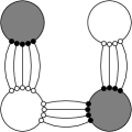
1 perm.

4 perm.

4 perm.

Figure 1: Spherical diagrams for the four-point correlator. The charges of the depicted operators are $J_{1}=4$, $J_{2}=9$, $K_{1}=5$, $K_{2}=8$. In the left diagram the number of lines, $a=2$, between $J_{1}$ and $K_{1}$ is not fixed. In the middle diagram the distribution of lines between $J_{2}$ and $K_{2}$ is not fixed. The right diagram is unique. Furthermore, permutations of the four operators must be taken into account.

Unlike the case of two- or three-point functions, the space-time dependence of eq.(2.2) is no longer fixed by conformal invariance. This can already be seen in free field theory. Consider fig. 1, which illustrates the three distinct types of possible planar Wick contractions of the four operators. It is clear that we have to sum over the number $a$ of contractions connecting the operators ${\cal O}^{J_{1}}(x_{1})$ and $\bar{\cal O}^{K_{1}}(y_{1})$. The corresponding space-time weight factor is

$$D^{J_{1}J_{2},K_{1}K_{2};a}_{x_{1}x_{2},y_{1}y_{2}}=\frac{1}{(x_{1}-y_{1})^{2a}(x_{1}-y_{2})^{2J_{1}-2a}(x_{2}-y_{1})^{2K_{1}-2a}(x_{2}-y_{2})^{2J_{2}-2K_{1}+2a}}$$ (2.3)

which can be also be written as

$$D^{J_{1}J_{2},K_{1}K_{2};a}_{x_{1}x_{2},y_{1}y_{2}}=D^{J_{1}J_{2},K_{1}K_{2};0}_{x_{1}x_{2},y_{1}y_{2}}~{}q^{a}$$ (2.4)

where

$$q=q_{x_{1}x_{2},y_{1}y_{2}}=\frac{(x_{1}-y_{2})^{2}(x_{2}-y_{1})^{2}}{(x_{1}-y_{1})^{2}(x_{2}-y_{2})^{2}}.$$ (2.5)

For the first class of diagrams in fig. 1 there is one way to distribute the lines for a given $a$, so the contribution is

$$\sum_{a=1}^{J_{1}-1}D^{J_{1}J_{2},K_{1}K_{2};a}_{x_{1}x_{2},y_{1}y_{2}}=D^{J_{1}J_{2},K_{1}K_{2};0}_{x_{1}x_{2},y_{1}y_{2}}\sum_{a=1}^{J_{1}-1}q^{a}=D^{J_{1}J_{2},K_{1}K_{2};0}_{x_{1}x_{2},y_{1}y_{2}}\,\frac{q^{J_{1}}-q}{q-1}$$ (2.6)

or $(J_{1}-1)D^{J_{1}J_{2},K_{1}K_{2};0}_{x_{1}x_{2},y_{1}y_{2}}$ for $q=1$. For the second class $a$ must be either $0$ or $J_{1}$ and there are $K_{2}-J_{1}$ or $K_{1}-J_{1}$ lines, respectively, to be distributed on two multi-lines. The contribution is thus (making use of $J_{1}+J_{2}=K_{1}+K_{2}$)

$$(J_{2}-K_{1}-1)~{}D^{J_{1}J_{2},K_{1}K_{2};0}_{x_{1}x_{2},y_{1}y_{2}}+(J_{2}-K_{2}-1)~{}D^{J_{1}J_{2},K_{1}K_{2};J_{1}}_{x_{1}x_{2},y_{1}y_{2}}.$$ (2.7)

The third class contributes a single diagram for $a=0$ and $a=J_{1}$, i.e. $D^{J_{1}J_{2},K_{1}K_{2};0}_{x_{1}x_{2},y_{1}y_{2}}+D^{J_{1}J_{2},K_{1}K_{2};J_{1}}_{x_{1}x_{2},y_{1}y_{2}}$. Furthermore, there are overall factors of $J_{1}$, $J_{2}$, $K_{1}$, $K_{2}$ to account for the different ways to connect the lines to the $Z$s inside the traces. Putting everything together, we find, for finite $J$, and to leading order in $N$ and $g_{\scriptscriptstyle\mathrm{YM}}^{2}$, the correlator $G^{J_{1}J_{2},K_{1}K_{2}}_{x_{1}x_{2},y_{1}y_{2}}$ to equal

$$\frac{\sqrt{J_{1}J_{2}K_{1}K_{2}}}{N^{2}}\,\left(\frac{q^{J_{1}}-q}{q-1}+(J_{2}-K_{1})+(J_{2}-K_{2})~{}q^{J_{1}}\right)D^{J_{1}J_{2},K_{1}K_{2};0}_{x_{1}x_{2},y_{1}y_{2}}.$$ (2.8)

We can now take the large $J$ limit, keeping the space-time structure fixed, as originally proposed in [1]. Here we must distinguish the cases $q<1$, $q=1$ and $q>1$ due to the exponential $q^{J_{1}}$. For $q\leq 1$ we take $D^{J_{1}J_{2},K_{1}K_{2};0}_{x_{1}x_{2},y_{1}y_{2}}$ as the space-time factor, for $q\geq 1$ we take $D^{J_{1}J_{2},K_{1}K_{2};J_{1}}_{x_{1}x_{2},y_{1}y_{2}}$ to absorb the divergent terms $q^{J_{1}}$, for $q=1$ both factors actually match. The large $J$ limit is

$$G^{J_{1}J_{2},K_{1}K_{2}}_{x_{1}x_{2},y_{1}y_{2}}=\frac{\sqrt{J_{1}J_{2}K_{1}K_{2}}}{N^{2}}\begin{cases}\hfill(J_{2}-K_{1})~{}D^{J_{1}J_{2},K_{1}K_{2};0}_{x_{1}x_{2},y_{1}y_{2}}&\mbox{for }q<1,\\ \hfill J_{2}~{}D^{J_{1}J_{2},K_{1}K_{2};0}_{x_{1}x_{2},y_{1}y_{2}}&\mbox{for }q=1,\\ \hfill(J_{2}-K_{2})~{}D^{J_{1}J_{2},K_{1}K_{2};J_{1}}_{x_{1}x_{2},y_{1}y_{2}}&\mbox{for }q>1.\\ \end{cases}$$ (2.9)

Note that the result for the correlator depends on whether the conformal ratio $q=q_{x_{1}x_{2},y_{1}y_{2}}$, which is a continuous function of the four positions $x_{1}$,$x_{2}$,$y_{1}$,$y_{2}$, is smaller, equal or larger than one. Moreover, this dependence is non-analytic, and actually discontinuous. In particular, this discontinuity is seen if we consider the pinching limit $x_{1}\rightarrow x_{2}$, $y_{1}\rightarrow y_{2}$. Nevertheless the discontinuity is not only seen when pinching: E.g. one has $q=1$ when the four points are located at the four corners of a perfect tetrahedron. Upon slightly dislocating any single one of the operators the correlation will jump. We did not investigate the free, planar four-point functions of BMN operators with impurities. However, we believe that the above discontinuities will plague these operators as well.

2.3 Planar, one-loop radiative corrections

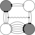
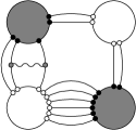
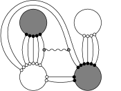
Figure 2: Planar diagrams of four-point correlators with leading radiative corrections. The wiggly line represents the sum of all radiative contributions within a face of the diagram, as explained in detail in appendix A. Diagrams like the ones on the top line contribute while diagrams on the bottom line do not.

Here we will investigate the leading ${\cal O}(g_{\scriptscriptstyle\mathrm{YM}}^{2})$ quantum corrections to the above four-point functions of chiral primary operators, at the planar level and in the BMN limit. This is interesting since it is well known that, even though the operators (2.1) are “protected”, quantum corrections are only absent at the level of two- and three-point functions. Four-point functions of such operators are, generically, not protected. The reason is that unprotected operators appear in intermediate channels of the correlation functions. Of course one might have hoped that such corrections are suppressed in the BMN limit. This will turn out to be not the case. Worse, we shall find that the quantum corrections are infinite in the BMN limit.

To compute the planar one-loop correction to the free, planar four-point correlator eq.(2.8) we have to “decorate” the diagrams of fig. 1 with either one one-loop self-energy insertion, one scalar four-point interaction, or one scalar-scalar gluon exchange. Planarity allows to reorganize the diagrammatics such that an effective “gluon” interaction, containing the combined effect of all these diagrams, affects all scalar lines bounding a face of the free diagram. The details of this calculation are deferred to appendix A. It is then demonstrated that only the first class of diagrams in fig. 1 has non-vanishing radiative corrections, which result from the effective interaction of the two quadrangles (four-gons) of the box-type diagrams. The effective interactions for all two-gons, as well as those for all faces of the other two classes of diagrams in fig. 1, vanish. The situation is schematically illustrated in fig. 2. The result for the quantum correction to the free correlator eq.(2.8) (cf appendix A) reads

$$\delta G^{J_{1}J_{2},K_{1}K_{2}}_{x_{1}x_{2},y_{1}y_{2}}=-\frac{\sqrt{J_{1}J_{2}K_{1}K_{2}}}{N^{2}}\,\frac{g_{\scriptscriptstyle\mathrm{YM}}^{2}N}{8\pi^{2}}\,\frac{q^{J_{1}}-q}{q-1}\,\mathnormal{\Phi}(r,s)\,D^{J_{1}J_{2},K_{1}K_{2};0}_{x_{1}x_{2},y_{1}y_{2}}~{}$$ (2.10)

where $D^{J_{1}J_{2},K_{1}K_{2};0}_{x_{1}x_{2},y_{1}y_{2}}$ is given, as before, by eq.(2.3) (with $a=0$) and the conformal ratio $q$ by eq.(2.5). The function $\mathnormal{\Phi}(r,s)$, whose explicit form is given in appendix A, is a complicated but finite function of the remaining conformal ratios $r,s$ (only two of the three ratios $q,r,s$ are independent):

$$r=r_{x_{1}x_{2},y_{1}y_{2}}=\frac{(x_{1}-y_{1})^{2}(x_{2}-y_{2})^{2}}{(x_{1}-x_{2})^{2}(y_{1}-y_{2})^{2}},\quad s=s_{x_{1}x_{2},y_{1}y_{2}}=\frac{(x_{1}-y_{2})^{2}(x_{2}-y_{1})^{2}}{(x_{1}-x_{2})^{2}(y_{1}-y_{2})^{2}}.$$ (2.11)

Now we are ready to investigate the the BMN limit $J\rightarrow\infty$ of this leading radiative correction. As for the free case we find a discontinuity at $q=1$:

$$\delta G^{J_{1}J_{2},K_{1}K_{2}}_{x_{1}x_{2},y_{1}y_{2}}=-\frac{\sqrt{J_{1}J_{2}K_{1}K_{2}}}{N^{2}}\,\frac{g_{\scriptscriptstyle\mathrm{YM}}^{2}}{8\pi^{2}}\,\mathnormal{\Phi}(r,s)~{}N\begin{cases}\frac{q}{1-q}~{}D^{J_{1}J_{2},K_{1}K_{2};0}_{x_{1}x_{2},y_{1}y_{2}}&\mbox{for }q<1,\\ \,\,\,J_{1}~{}D^{J_{1}J_{2},K_{1}K_{2};0}_{x_{1}x_{2},y_{1}y_{2}}&\mbox{for }q=1,\\ \frac{1}{q-1}~{}D^{J_{1}J_{2},K_{1}K_{2};J_{1}}_{x_{1}x_{2},y_{1}y_{2}}&\mbox{for }q>1.\\ \end{cases}$$ (2.12)

Actually, the discontinuity is now even worse since the power of $J$ changes in a discrete fashion as $q\rightarrow 1$. Furthermore, we see that the quantum correction $\delta G^{J_{1}J_{2},K_{1}K_{2}}_{x_{1}x_{2},y_{1}y_{2}}$ diverges relative to the classical contribution $G^{J_{1}J_{2},K_{1}K_{2}}_{x_{1}x_{2},y_{1}y_{2}}$ in the BMN limit: The extra power of $N$ in eq.(2.12) scales as $N\sim J^{2}$. For $q=1$ the divergence is therefore quadratic in $J$, while for $q\neq 1$ it is linear in $J$.

It is interesting to check the “double-pinching” limit $x_{1}\rightarrow x_{2}$, $y_{1}\rightarrow y_{2}$ of eq.(2.10) before taking the BMN limit: In this case the function $\mathnormal{\Phi}(r,s)$ vanishes, and there are no quantum corrections at all. This is easy to understand, since we then effectively compute a two-point function of protected double-trace operators $\bigl{\langle}{\cal O}^{J_{1}}{\cal O}^{J_{2}}(x_{1})\bar{\cal O}^{K_{1}}\bar{\cal O}^{K_{2}}(y_{1})\bigr{\rangle}$.

One expects the above result to also hold for BMN operators with impurities. We conclude that the BMN limit of $\mathcal{N}=4$ perturbative Super Yang-Mills theory does not appear to be meaningful for general correlation functions of BMN operators. The above discontinuity and divergence properties cast some doubts on attempts to relate Yang-Mills $n$-point functions to $n$-string amplitudes. This is consistent with the picture proposed in [11] that one should only compare two-point functions of multi-trace operators to multi-string amplitudes. We feel that our result also questions the validity of the proposal of [10] that relates the Yang-Mills three-point function to the string three-vertex: The information obtained from the three-field correlator of BMN operators can also be obtained by pinching the three-point function before taking the BMN limit and subsequently extracting the amplitude from the resulting two-point function. This is again in accordance with the proposal of [11].

2.4 Double-scaled free field theory result (at $q=1$)

So far we have only considered the correlation function eq.(2.2) in the strict planar limit, as in [1], exposing two types of obstructions to a meaningful BMN limit for four-point functions. For completeness, we would like to discuss the structure of free, non-planar contributions to these correlators. As originally shown in [8], these are generically finite and non-vanishing in the BMN limit. This remains true for the four-point function eq.(2.2). Indeed, using the methods of [8], it is straightforward to work out the non-planar, free-field corrections to eq.(2.9). E.g. the torus correction reads

$$\delta_{\frac{1}{N^{2}}}G^{J_{1}J_{2},K_{1}K_{2}}_{x_{1}x_{2},y_{1}y_{2}}=G^{J_{1}J_{2},K_{1}K_{2}}_{x_{1}x_{2},y_{1}y_{2}}~{}\frac{1}{24N^{2}}\begin{cases}\frac{J(K_{1}^{4}-K_{2}^{4})+2J_{1}J_{2}(K_{1}^{3}-K_{2}^{3})}{K_{1}-K_{2}}&\mbox{for }q\neq 1\\ J_{1}^{2}J^{2}+J_{2}^{2}(K_{1}^{2}+K_{2}^{2})&\mbox{for }q=1.\\ \end{cases}$$ (2.13)

We observe that the intriguing discontinuities found above continue to be present at ${\cal O}(\frac{1}{N^{2}})$. For $q=1$ we can, extending our results in [8], go further and find, using matrix model techniques, the complete $\frac{1}{N}$ expansion of the free-field contribution to the four-point function. The result (see appendix B) reads

$$G^{J_{1}J_{2},K_{1}K_{2}}_{x_{1}x_{2},y_{1}y_{2}}\Big{|}^{q=1}_{{\rm free}}=D^{J_{1}J_{2},K_{1}K_{2};0}_{x_{1}x_{2},y_{1}y_{2}}\,\frac{4J}{\sqrt{J_{1}J_{2}K_{1}K_{2}}}\,\frac{\sinh\frac{JJ_{1}}{2N}\,\sinh\frac{J_{2}K_{1}}{2N}\,\sinh\frac{J_{2}K_{2}}{2N}}{\frac{J^{2}}{2N}}.$$ (2.14)

The result shows that the “scaling functions”, discovered in [8], also appear in the description of the free field limit of non-extremal four-point functions of chiral primaries to all orders in the effective coupling constant $g_{2}=\frac{J^{2}}{N}$. A puzzling question is whether all-genus expressions such as eq.(2.14) have an interpretation on the string side. According to [10, 11] this should not be the case: These authors argue that the true string interactions always come with a factor $\sqrt{\lambda^{\prime}}\frac{J^{2}}{N}$ where $\lambda^{\prime}=g_{\scriptscriptstyle\mathrm{YM}}^{2}\frac{N}{J^{2}}$, and that the above free non-planar corrections should be absorbed in the gauge-string dictionary. For chiral operators, this dictionary seems to be highly non-unique if we allow for general operator mixing (see section 3.5); we feel that the issue should be understood much better.

3 Two-point functions, operator mixing and one-loop toroidal anomalous dimensions

3.1 General remarks

In the previous chapter we demonstrated that the quantum corrections to the generic space-time correlation function of the chiral primary operators ${\cal O}^{J}=\frac{1}{\sqrt{J}}\bigl{(}\frac{8\pi^{2}}{g_{\scriptscriptstyle\mathrm{YM}}^{2}N}\bigr{)}^{J/2}\mathop{\mathrm{Tr}}Z^{J}$, $Z=\frac{1}{\sqrt{2}}(\phi_{5}+i\phi_{6})$, defined in eq.(2.1) are divergent in the BMN limit (1.1), in line with naive expectation. This problem does not appear at the level of two- and three-point functions of these operators, which are protected against quantum corrections. An interesting slight modification of the operators ${\cal O}^{J}$ was invented in [1]: If one inserts two “defect fields”, e.g. two of the scalar fields $\phi_{i}$ ($i=1,2,3,4$) not appearing in eq.(2.1), at two arbitrary positions inside the trace, the resulting operators ($i\neq j$)

$${\cal O}^{J,p}_{ij}=\left(\frac{8\pi^{2}}{g_{\scriptscriptstyle\mathrm{YM}}^{2}N}\right)^{J/2+1}\mathop{\mathrm{Tr}}(\phi_{i}Z^{p}\phi_{j}Z^{J-p})\qquad{\rm with}\qquad p=0,1,\ldots,J$$ (3.1)

are no longer protected; however, for very large $J$ one could expect the resulting quantum effects to be small. In free field theory, and in the planar limit, the operators (3.1) are orthonormal. Computing their planar two-point function at one loop this is no longer the case, since interactions can exchange the positions of the fields $\phi_{i}$ and the adjacent fields $Z$, leading to operator mixing between the fields ${\cal O}^{J,p}_{ij}$. However, by a linear transformation the fields can be diagonalized at the planar and one-loop level, resulting in the BMN operators [1]:

$${\cal O}^{J}_{ij,n}(x)=\frac{1}{\sqrt{J}}\sum_{p=0}^{J}e^{2\pi ip\,n/J}~{}{\cal O}^{J,p}_{ij}(x).$$ (3.2)

After ensuring orthogonality of the operators one may extract their scaling dimension $\Delta_{n}$ from the two-point function

$$\bigl{\langle}{\cal O}^{J}_{ij,m}(x)\,\bar{\cal O}^{J}_{ij,n}(0)\bigr{\rangle}=\frac{\delta_{mn}}{|x|^{2\Delta_{n}}}.$$ (3.3)

It is anomalous since for $n\neq 0$ it deviates in the quantum theory by $(\delta\Delta_{n})$ from the classical dimension $J+2$:

$$\Delta_{n}=J+2+(\delta\Delta_{n}).$$ (3.4)

At one loop, and in the planar limit, one has [1]

$$(\delta\Delta_{n})=\lambda^{\prime}n^{2}$$ (3.5)

where $\lambda^{\prime}$ is finite in the BMN limit, see (1.1),(1.2). The orthogonalization (3.2) appears to be valid, at large $J$, and at the planar level, to all orders in the coupling, and the exact planar anomalous dimension is believed to be known [1, 2, 3]. Technically, the one-loop anomalous dimension is obtained as follows. Computing in one-loop perturbation theory the correction to the free result one finds

$$\bigl{\langle}{\cal O}^{J}_{ij,m}(x)\,\bar{\cal O}^{J}_{ij,n}(0)\bigr{\rangle}=\frac{\delta_{mn}}{|x|^{2J+4}}\,\bigl{(}1+(\delta\Delta_{n})~{}L\bigr{)}$$ (3.6)

where $L=\log(x\Lambda)^{-2}$. Clearly $L$ reproduces the expected $x$-dependence when expanding the definition eq.(3.3), using eq.(3.4); $\log\Lambda^{2}$ is a divergent constant (depending on the regularization scheme employed) that sets the scale. More details can be found in appendix C.

For the remainder of this chapter we will shorten the notation by omitting the $x$-dependence of the correlators as well as the multiplicative factors $\frac{g_{\scriptscriptstyle\mathrm{YM}}^{2}}{8\pi^{2}}$ from the scalar propagators and operator normalizations in (3.1). In these conventions eq.(3.6) compactly reads

$$\bigl{\langle}{\cal O}^{J}_{ij,m}\bar{\cal O}^{J}_{ij,n}\bigr{\rangle}=\delta_{mn}~{}\bigl{(}1+(\delta\Delta_{n})~{}L\bigr{)}.$$ (3.7)

It is natural to ask for the non-planar corrections to the anomalous dimensions eq.(3.5). Important steps in this direction were undertaken in [8, 10], where the genus one classical and one-loop quantum corrections to the correlator eq.(3.7) were computed. The result reads, putting e.g. $i=1,j=2$

$$\bigl{\langle}{\cal O}^{J}_{12,m}\,\bar{\cal O}^{J}_{12,n}\bigr{\rangle}\mathrel{} = \mathrel{}\delta_{mn}\left(1+\frac{\lambda^{\prime}L}{8\pi^{2}}\,8\pi^{2}m^{2}\right)$$ (3.8)

$$\mathord{}+g_{2}^{2}\,\left(M^{1}_{mn}+\frac{\lambda^{\prime}L}{8\pi^{2}}\left(8\pi^{2}mnM^{1}_{mn}+{\mathcal{D}^{1}_{mn}}\right)\right)$$

$$\mathord{}+\mathcal{O}(g_{2}^{4})$$

where the matrices $M^{1}_{mn}$, ${\mathcal{D}^{1}_{mn}}$ can be found in appendix E (the notation is the one of [8], except for the additional upper index $1$ on the matrices in the present paper). As was already discussed in detail in [8, 10], on the torus the operators eq.(3.2) are no longer orthogonal classically: The matrix $M^{1}_{mn}$ is not diagonal. By a linear transformation we could proceed to (i) orthonormalize the classical contribution in eq.(3.8) and (ii) subsequently diagonalize the quantum contribution by an orthogonal transformation; this would not affect the classical part which would be already proportional to the unit matrix $\delta_{mn}$ after step (i). This is nevertheless not correct. The reason is easy to understand pictorially: Considering the torus correction to a two-point function, we see from fig. 3 that double-trace operators appear in intermediate channels. And indeed, as we shall find in the next section, the overlap between such double-trace operators and the single-trace BMN operators is of ${\cal O}(g_{2})$. It therefore affects the ${\cal O}(g_{2}^{2})$ anomalous dimension upon diagonalization. We conclude that the calculations of [8, 10] are not quite complete, and we will now proceed to derive the correct dimensions.

Figure 3: Cutting the torus of a correlator between two single trace operators yields double trace operators. The two impurities can either be on the same branch or on different branches corresponding to ${\cal T}^{J,r}_{ij,n}$ and ${\cal T}^{J,r}_{ij}$ of (3.10), respectively.

3.2 Operator definitions

Let us recapitulate and slightly extend the definitions of the properly normalized BMN operators with, respectively, zero, one and two impurities:

$${\cal O}^{J}\mathrel{} = \mathrel{}\frac{1}{\sqrt{J\,N^{J}}}\,\mathop{\mathrm{Tr}}\,Z^{J},$$

$${\cal O}^{J}_{i}\mathrel{} = \mathrel{}\frac{1}{\sqrt{N^{J+1}}}\,\mathop{\mathrm{Tr}}\bigl{(}\phi_{i}\,Z^{J}\bigr{)},$$ (3.9)

$${\cal O}^{J}_{ij,n}\mathrel{} = \mathrel{}\frac{1}{\sqrt{J\,N^{J+2}}}\left(\sum_{p=0}^{J}e^{2\pi ip\,n/J}\mathop{\mathrm{Tr}}\bigl{(}\phi_{i}\,Z^{p}\,\phi_{j}\,Z^{J-p}\bigr{)}-\delta_{ij}\mathop{\mathrm{Tr}}\bigl{(}\bar{Z}Z^{J+1}\bigr{)}\right).$$

Recall that we shortened the notation by omitting the $x$-dependence of the operators and correlators, and by setting all multiplicative factors $\frac{g_{\scriptscriptstyle\mathrm{YM}}^{2}}{8\pi^{2}}$ to one. Both dependencies are trivially restored if needed, cf section 3.1. The last operator has been slightly generalized as compared to eq.(3.2) in order to also allow for the insertions of two impurities of the same kind (i.e. $i=j$). This was derived in detail in [25]. As we just argued we should also include double-trace operators (see also [22]). The ones we need (see fig. 3) are defined as

$${\cal T}^{J,r}\mathrel{} = \mathrel{}{\cal O}^{r\cdot J}\,{\cal O}^{(1-r)\cdot J},$$

$${\cal T}^{J,r}_{i}\mathrel{} = \mathrel{}{\cal O}^{r\cdot J}_{i}\,{\cal O}^{(1-r)\cdot J},$$

$${\cal T}^{J,r}_{ij,n}\mathrel{} = \mathrel{}{\cal O}^{r\cdot J}_{ij,n}\,{\cal O}^{(1-r)\cdot J},$$

$${\cal T}^{J,r}_{ij}\mathrel{} = \mathrel{}{\cal O}^{r\cdot J}_{i}\,{\cal O}^{(1-r)\cdot J}_{j}.$$ (3.10)

Here $r=\frac{J^{\prime}}{J}$ where $J^{\prime}$ is taken in the range $J^{\prime}=1,\ldots,J-1$. In the BMN limit $r$ can be thought of as a real number in the range $r\in(0,1)$.

The operators ${\cal O}^{J}$ and ${\cal T}^{J,r}$ are SO(4) singlets and the operators ${\cal O}^{J}_{i}$ and ${\cal T}^{J,r}_{i}$ are SO(4) vectors. Operators containing two scalar defects should be decomposed into the SO(4) irreps $\mathbf{9}+\mathbf{6}+\mathbf{1}$. They correspond to the symmetric-traceless, anti-symmetric and singlet representations:

$${\cal O}^{J}_{(ij),n}\mathrel{} = \mathrel{}{\textstyle\frac{1}{2}}\bigl{(}{\cal O}^{J}_{ij,n}+{\cal O}^{J}_{ji,n}\bigr{)}-{\textstyle\frac{1}{4}}\,\delta_{ij}{\textstyle\sum}_{k}{\cal O}^{J}_{kk,n},$$

$${\cal O}^{J}_{[ij],n}\mathrel{} = \mathrel{}{\textstyle\frac{1}{2}}\bigl{(}{\cal O}^{J}_{ij,n}-{\cal O}^{J}_{ji,n}\bigr{)},\qquad\qquad$$

$${\cal O}^{J}_{{\mathbf{1}},n}\mathrel{} = \mathrel{}{\textstyle\frac{1}{2}}{\textstyle\sum}_{k}{\cal O}^{J}_{kk,n}.$$ (3.11)

Note that due to the identity ${\cal O}^{J}_{ij,-n}={\cal O}^{J}_{ji,n}$ the operators in (3.11) with negative mode number $-n$ equal the operators with positive mode number $n$ up to a sign for the anti-symmetric operator

$${\cal O}^{J}_{(ij),-n}={\cal O}^{J}_{(ij),n},\quad{\cal O}^{J}_{[ij],-n}=-{\cal O}^{J}_{[ij],n},\quad{\cal O}^{J}_{{\mathbf{1}},-n}={\cal O}^{J}_{{\mathbf{1}},n}.$$ (3.12)

Clearly the zero-mode operators exist only in the symmetric-traceless and singlet representations, they are protected half BPS operators. Nevertheless, we prefer not to implement the decomposition into symmetric and anti-symmetric parts in the course of our calculation: This would lead to Fourier-sine and Fourier-cosine series instead of the more convenient ordinary Fourier series. We therefore continue to work with ${\cal O}^{J}_{12,n}$ to capture the anomalous dimension of the (redefined) $\mathbf{9}+\mathbf{6}$ operators (section 3.3) according to

$$\bigl{\langle}\bar{\cal O}^{J}_{12,n}\,{\cal O}^{J}_{12,m}\bigr{\rangle}=\delta_{mn}+\delta_{mn}\frac{\delta\Delta_{n}^{\mathbf{9}}+\delta\Delta_{n}^{\mathbf{6}}}{2}\,L+\delta_{m,-n}\frac{\delta\Delta_{n}^{\mathbf{9}}-\delta\Delta_{n}^{\mathbf{6}}}{2}\,L.$$ (3.13)

The singlet operator ${\cal O}^{J}_{{\mathbf{1}},n}$ needs to be considered separately (section 3.4).

3.3 Symmetric and anti-symmetric BMN operators

Next one computes the two-point functions of one- and two-trace operators at the tree and one-loop level, up to ${\cal O}(g_{2}^{2})$. These computations are efficiently performed using the techniques of appendices C or D, which reduce the problem to a purely combinatorial one. We already stated the known result for the overlap of single-trace operators, eq.(3.8). The analogous expressions for double-trace operators are only needed to leading order in $g_{2}$ and are therefore simpler:

$$\bigl{\langle}{\cal T}^{J,r}_{12}\,\bar{\cal T}^{J,s}_{12}\bigr{\rangle}\mathrel{} = \mathrel{}\delta_{rs}+\mathcal{O}(g_{2}^{2}),$$

$$\bigl{\langle}{\cal T}^{J,r}_{12,m}\,\bar{\cal T}^{J,s}_{12,n}\bigr{\rangle}\mathrel{} = \mathrel{}\delta_{rs}\delta_{mn}\left(1+\frac{\lambda^{\prime}L}{8\pi^{2}}\,\frac{8\pi^{2}m^{2}}{r^{2}}\right)+\mathcal{O}(g_{2}^{2}),$$

$$\bigl{\langle}{\cal T}^{J,r}_{12,m}\,\bar{\cal T}^{J,s}_{12}\bigr{\rangle}\mathrel{} = \mathrel{}\mathcal{O}(g_{2}^{2}).$$ (3.14)

The overlaps between single- and double-trace operators turn out to be

$$\bigl{\langle}{\cal T}^{J,r}_{12,m}\,\bar{\cal O}^{J}_{12,n}\bigr{\rangle}\mathrel{} = \mathrel{}\frac{g_{2}\,r^{3/2}\sqrt{1-r}\sin^{2}(\pi nr)}{\sqrt{J}\,\pi^{2}(m-nr)^{2}}$$

$$\mathord{}\qquad\qquad\times\left(1+\frac{\lambda^{\prime}L}{8\pi^{2}}\,\frac{8\pi^{2}(m^{2}-mnr+n^{2}r^{2})}{r^{2}}\right)+\mathcal{O}(g_{2}^{3}),$$

$$\bigl{\langle}{\cal T}^{J,r}_{12}\,\bar{\cal O}^{J}_{12,n}\bigr{\rangle}\mathrel{} = \mathrel{}\frac{g_{2}}{\sqrt{J}}\left(\delta_{n,0}\,r-\frac{\sin^{2}(\pi nr)}{\pi^{2}\,n^{2}}\right)\left(1+\frac{\lambda^{\prime}L}{8\pi^{2}}\,8\pi^{2}n^{2}\right)+\mathcal{O}(g_{2}^{3}).$$

The classical parts were already found in [10] and the one-loop results for the special case $m=0$ were presented in [4]. As we mentioned above these overlaps are of $\mathcal{O}(g_{2})$. To correctly diagonalize we have to remove the overlap by a redefinition of the single and double trace operators

$${\cal O}^{\prime\,J}_{12,m}\mathrel{} = \mathrel{}{\cal O}^{J}_{12,m}-\sum_{k,r}\frac{g_{2}\,r^{3/2}\sqrt{1-r}\,\sin^{2}(\pi mr)\,k}{\sqrt{J}\,\pi^{2}(k-mr)^{2}(k+mr)}\,{\cal T}^{J,r}_{12,k},$$

$${\cal T}^{\prime\,J,r}_{12,m}\mathrel{} = \mathrel{}{\cal T}^{J,r}_{12,m}-\sum_{k}\frac{g_{2}\,r^{3/2}\sqrt{1-r}\,\sin^{2}(\pi kr)\,kr}{\sqrt{J}\,\pi^{2}(m-kr)^{2}(m+kr)}\,{\cal O}^{J}_{12,k},$$

$${\cal T}^{\prime\,J,r}_{12}\mathrel{} = \mathrel{}{\cal T}^{J,r}_{12}-\sum_{k}\frac{g_{2}}{\sqrt{J}}\left(\delta_{k,0}\,r-\frac{\sin^{2}(\pi kr)}{\pi^{2}k^{2}}\right){\cal O}^{J}_{12,k}$$ (3.16)

where the sums go over all integers $k$ and all $r=J^{\prime}/J$ with $1\leq J^{\prime}\leq J-1$; i.e. the redefinitions are chosen such that

$$\bigl{\langle}{\cal T}^{\prime\,J,r}_{12,m}\,\bar{\cal O}^{\prime\,J}_{12,n}\bigr{\rangle}\mathrel{} = \mathrel{}\mathcal{O}(g_{2}^{3}),$$

$$\bigl{\langle}{\cal T}^{\prime\,J,r}_{12}\,\bar{\cal O}^{\prime\,J}_{12,n}\bigr{\rangle}\mathrel{} = \mathrel{}\mathcal{O}(g_{2}^{3}).$$ (3.17)

The eqs.(3.16) are unique since we need to eliminate both the leading ${\cal O}(g_{2})$ classical as well as the leading ${\cal O}(g_{2}\lambda^{\prime}L)$ one-loop overlaps, cf eq.(LABEL:double-single).

The redefined single trace correlator receives corrections from the double trace part

$$\bigl{\langle}{\cal O}^{\prime\,J}_{12,m}\bar{\cal O}^{\prime\,J}_{12,n}\bigr{\rangle}$$

$$= \mathrel{}\delta_{mn}\left(1+\frac{\lambda^{\prime}L}{8\pi^{2}}\,8\pi^{2}m^{2}\right)+g_{2}^{2}\left(M_{mn}^{1}+\frac{\lambda^{\prime}L}{8\pi^{2}}\left(8\pi^{2}mnM^{1}_{mn}+\mathcal{D}^{1}_{mn}\right)\right)$$

$$\mathord{}-g_{2}^{2}\sum_{k,r}\frac{r^{3}(1-r)\sin^{2}(\pi mr)\sin^{2}(\pi nr)\,k}{J\pi^{4}(k-mr)^{2}(k+mr)(k-nr)^{2}(k+nr)}$$

$$\mathord{}\qquad\times\left(k+mr+nr+\frac{\lambda^{\prime}L}{8\pi^{2}r^{2}}\,8\pi^{2}\left(k^{3}+m^{3}r^{3}+n^{3}r^{3}\right)\right)$$

$$= \mathrel{}\delta_{mn}\left(1+\frac{\lambda^{\prime}L}{8\pi^{2}}\,8\pi^{2}m^{2}\right)+g_{2}^{2}\left(M_{mn}+\frac{\lambda^{\prime}L}{8\pi^{2}}\,\left(8\pi^{2}mnM_{mn}+\mathcal{D}_{mn}\right)\right)$$

where we have defined

$$M_{mn}=M^{1}_{mn}+M^{2}_{mn},\qquad\mathcal{D}_{mn}=\mathcal{D}^{1}_{mn}+\mathcal{D}^{2}_{mn},$$ (3.18)

and where the matrix elements $M^{2}_{mn}$, $\mathcal{D}^{2}_{mn}$ are derived by computing the above double sum in the BMN limit. Their detailed form can be found in appendix E. Care has to be taken to correctly treat the special cases $|m|=|n|$, which are the ones that are directly relevant to the numerical values of the toroidal anomalous dimensions. The off-diagonal pieces are, however, needed as well. They are part of the precise dictionary since we have to work with an orthonormal set of operators in order to read off the one-loop correction to the anomalous dimension, cf the discussion around eq.(3.6). We therefore linearly redefine the ${\cal O}^{\prime\,J}_{12,n}$ once more, employing the off-diagonal elements:

$${\cal O}^{\prime\prime\,J}_{12,m}={\cal O}^{\prime\,J}_{12,m}+g_{2}^{2}\,\sum_{k}T_{mk}\,{\cal O}^{\prime\,J}_{12,k}$$ (3.19)

with (here $|n|\neq|k|$)

$$T_{nn}=-\frac{M_{nn}}{2},\quad T_{n,-n}=-\frac{M_{n,-n}}{2},\quad T_{nk}=-\frac{nM_{nk}}{n+k}+\frac{\mathcal{D}_{nk}}{8\pi^{2}(n^{2}-k^{2})}.$$ (3.20)

This redefinition is chosen in order to remove the overlap between impurity operators ${\cal O}^{\prime\prime\,J}_{12,m}$ and $\bar{\cal O}^{\prime\prime\,J}_{12,n}$ with $|n|\neq|m|$:

$$\bigl{\langle}{\cal O}^{\prime\prime\,J}_{12,m}\bar{\cal O}^{\prime\prime\,J}_{12,n}\bigr{\rangle}=\mathcal{O}(g_{2}^{4})\qquad\mbox{if }|m|\neq|n|$$ (3.21)

As was discussed above, a priori only the symmetric and anti-symmetric combinations ${\cal O}^{\prime\prime\,J}_{(12),n}$ and ${\cal O}^{\prime\prime\,J}_{[12],n}$ of eq.(3.11) are expected to have definite anomalous dimensions; therefore we should have $\bigl{\langle}{\cal O}^{\prime\prime\,J}_{12,n}\bar{\cal O}^{\prime\prime\,J}_{12,-n}\bigr{\rangle}\neq 0$. Surprisingly, we find, using eq.(3.18) and the results of appendix E,

$$\frac{\delta\Delta^{\mathbf{9}}_{n}-\delta\Delta^{\mathbf{6}}_{n}}{2}\,L=\bigl{\langle}{\cal O}^{\prime\prime\,J}_{12,n}\bar{\cal O}^{\prime\prime\,J}_{12,-n}\bigr{\rangle}=\frac{g_{2}^{2}\lambda^{\prime}}{8\pi^{2}}~{}(\mathcal{D}_{n,-n}-16\pi^{2}n^{2}M_{n,-n})L=0.$$ (3.22)

This involves a delicate conspiracy between the matrix elements $M_{n,-n}$ and $\mathcal{D}_{n,-n}$, which are, respectively, obtained from rather different calculations. It means that ${\cal O}^{\prime\prime\,J}_{(12),n}$ and ${\cal O}^{\prime\prime\,J}_{[12],n}$ have degenerate anomalous dimensions, and the operators ${\cal O}^{\prime\prime\,J}_{12,n}$ are completely one-loop orthogonal up to order $g_{2}^{2}$

$$\bigl{\langle}{\cal O}^{\prime\prime\,J}_{12,m}\bar{\cal O}^{\prime\prime\,J}_{12,n}\bigr{\rangle}\mathrel{} = \mathrel{}\delta_{mn}\left(1+\frac{\lambda^{\prime}L}{8\pi^{2}}\left(8\pi^{2}m^{2}+g_{2}^{2}~{}\mathcal{D}_{mm}\right)\right)$$ (3.23)

$$= \mathrel{}\delta_{mn}\Bigg{(}1+\frac{\lambda^{\prime}L}{8\pi^{2}}\bigg{(}8\pi^{2}m^{2}+g_{2}^{2}\Big{(}\frac{1}{6}+\frac{35}{16\pi^{2}m^{2}}\Big{)}\bigg{)}\Bigg{)},$$

(we used $\mathcal{D}_{mm}=\mathcal{D}^{1}_{mm}+\mathcal{D}^{2}_{mm}$ and appendix E) allowing us, in view of eqs.(3.4),(3.7), to read off their anomalous dimensions

$$\Delta^{\mathbf{9}}_{n}=\Delta^{\mathbf{6}}_{n}=J+2+\frac{\lambda^{\prime}}{8\pi^{2}}\left(8\pi^{2}n^{2}+g_{2}^{2}\left(\frac{1}{6}+\frac{35}{16\pi^{2}n^{2}}\right)\right)\quad(n\neq 0).$$ (3.24)

Put differently, operators in the SO(4) representations $\mathbf{9}$ and $\mathbf{6}$ possess degenerate anomalous dimensions. From the field theory point of view there is a priori no reason to believe that operators belonging to different representations should have equal anomalous dimensions. On the sphere it might have been a coincidence that the dimensions match, but on the torus it is a remarkable result. It would be interesting to understand the symmetry reason for this result.

3.4 Singlet BMN operators

Let us now turn to the determination of the anomalous dimension of the SO(4) singlet BMN operator with two impurities. Again the mixing of one- and two-trace operators needs to be taken into account. Here the computations are somewhat more involved as contributions from the “K-terms” of (C.14) coupling to traces need to be dealt with, see appendices C and D for details. Note, that now the inclusion of the $\mathop{\mathrm{Tr}}(\bar{Z}Z^{J+1})$ term for the diagonal operator ${\cal O}_{ii,n}^{J}$ of (3.9) is crucial: It precisely cancels terms violating the BMN scaling limit originating from the first “naive” piece of the operator ${\cal O}_{ii,n}^{J}$ in (3.9). We then find

$$\bigl{\langle}{\cal O}^{J}_{{\mathbf{1}},m}\,\bar{\cal O}^{J}_{{\mathbf{1}},n}\bigr{\rangle}\mathrel{} = \mathrel{}\bigl{\langle}{\cal O}^{J}_{12,m}\,\bar{\cal O}^{J}_{12,n}\bigr{\rangle}+\bigl{\langle}{\cal O}^{J}_{12,m}\,\bar{\cal O}^{J}_{12,-n}\bigr{\rangle}-\frac{\lambda^{\prime}L}{8\pi^{2}}\,2g_{2}^{2}\mathcal{D}^{1}_{mn}+\mathcal{O}(g_{2}^{4}),$$

$$\bigl{\langle}{\cal T}^{J,r}_{{\mathbf{1}},m}\,\bar{\cal O}^{J}_{{\mathbf{1}},n}\bigr{\rangle}\mathrel{} = \mathrel{}\bigl{\langle}{\cal T}^{J,r}_{12,m}\,\bar{\cal O}^{J}_{12,n}\bigr{\rangle}+\bigl{\langle}{\cal T}^{J,r}_{12,m}\,\bar{\cal O}^{J}_{12,-n}\bigr{\rangle}$$

$$\mathord{}-\,\frac{\lambda^{\prime}L}{8\pi^{2}}\,\frac{16g_{2}\sqrt{1-r}\sin^{2}(\pi nr)}{\sqrt{Jr}}+\mathcal{O}(g_{2}^{3}),$$

$$\bigl{\langle}{\cal T}^{J,r}_{{\mathbf{1}}}\,\bar{\cal O}^{J}_{{\mathbf{1}},n}\bigr{\rangle}\mathrel{} = \mathrel{}2\,\bigl{\langle}{\cal T}^{J,r}_{12}\,\bar{\cal O}^{J}_{12,n}\bigr{\rangle}+\frac{\lambda^{\prime}L}{8\pi^{2}}\,\frac{16g_{2}\sin^{2}(\pi nr)}{\sqrt{J}}+\mathcal{O}(g_{2}^{3}),$$

$$\bigl{\langle}{\cal T}^{J,r}_{{\mathbf{1}}}\,\bar{\cal T}^{J,s}_{{\mathbf{1}}}\bigr{\rangle}\mathrel{} = \mathrel{}\bigl{\langle}{\cal T}^{J,r}_{12}\,\bar{\cal T}^{J,s}_{12}\bigr{\rangle}+\bigl{\langle}{\cal T}^{J,r}_{12}\,\bar{\cal T}^{J,1-s}_{12}\bigr{\rangle}+\mathcal{O}(g_{2}^{2}),$$

$$\bigl{\langle}{\cal T}^{J,r}_{{\mathbf{1}},m}\,\bar{\cal T}^{J,s}_{{\mathbf{1}},n}\bigr{\rangle}\mathrel{} = \mathrel{}\bigl{\langle}{\cal T}^{J,r}_{12,m}\,\bar{\cal T}^{J,s}_{12,n}\bigr{\rangle}+\bigl{\langle}{\cal T}^{J,r}_{12,m}\,\bar{\cal T}^{J,s}_{12,-n}\bigr{\rangle}+\mathcal{O}(g_{2}^{2}),$$

$$\bigl{\langle}{\cal T}^{J,r}_{{\mathbf{1}},m}\,\bar{\cal T}^{K,s}_{{\mathbf{1}}}\bigr{\rangle}\mathrel{} = \mathrel{}\mathcal{O}(g_{2}^{2}).$$ (3.25)

where the contributions from $V_{F}$ arising from (C.14) reside in the correlator expressions in the right hand sides of the above and the contributions from the $V_{K}$ sector have been spelled out explicitly to the order needed. Making use of (3.8),(3.14) and (LABEL:double-single) one has

$$\bigl{\langle}{\cal O}^{J}_{{\mathbf{1}},m}\,\bar{\cal O}^{J}_{{\mathbf{1}},n}\bigr{\rangle}\mathrel{} = \mathrel{}\bigl{(}\delta_{mn}+\delta_{m,-n}\bigr{)}\left(1+\frac{\lambda^{\prime}L}{8\pi^{2}}\,8\pi^{2}m^{2}\right)$$

$$\mathord{}+g_{2}^{2}\,\left(M^{1}_{mn}+M^{1}_{m,-n}+\frac{\lambda^{\prime}L}{8\pi^{2}}8\pi^{2}mn\left(M^{1}_{mn}-M^{1}_{m,-n}\right)\right)$$

$$\mathord{}+\mathcal{O}(g_{2}^{4}),$$

$$\bigl{\langle}{\cal T}^{J,r}_{{\mathbf{1}},m}\,\bar{\cal O}^{J}_{{\mathbf{1}},n}\bigr{\rangle}\mathrel{} = \mathrel{}\frac{g_{2}\,r^{3/2}\sqrt{1-r}\sin^{2}(\pi nr)}{\sqrt{J}\,\pi^{2}(m-nr)^{2}}\left(1+\frac{\lambda^{\prime}L}{8\pi^{2}}\,\frac{8\pi^{2}mn}{r}\right)$$

$$\mathord{}+\frac{g_{2}\,r^{3/2}\sqrt{1-r}\sin^{2}(\pi nr)}{\sqrt{J}\,\pi^{2}(m+nr)^{2}}\left(1-\frac{\lambda^{\prime}L}{8\pi^{2}}\,\frac{8\pi^{2}mn}{r}\right)+\mathcal{O}(g_{2}^{3}),$$

$$\bigl{\langle}{\cal T}^{J,r}_{{\mathbf{1}}}\,\bar{\cal O}^{J}_{{\mathbf{1}},n}\bigr{\rangle}\mathrel{} = \mathrel{}\frac{2g_{2}}{\sqrt{J}}\left(\delta_{n,0}\,r-\frac{\sin^{2}(\pi nr)}{\pi^{2}\,n^{2}}\right)+\mathcal{O}(g_{2}^{3}),$$

$$\bigl{\langle}{\cal T}^{J,r}_{{\mathbf{1}}}\,\bar{\cal T}^{J,s}_{{\mathbf{1}}}\bigr{\rangle}\mathrel{} = \mathrel{}\delta_{rs}+\delta_{r,1-s}+\mathcal{O}(g_{2}^{2}),$$

$$\bigl{\langle}{\cal T}^{J,r}_{{\mathbf{1}},m}\,\bar{\cal T}^{J,s}_{{\mathbf{1}},n}\bigr{\rangle}\mathrel{} = \mathrel{}\delta_{rs}\bigl{(}\delta_{mn}+\delta_{m,-n}\bigr{)}\left(1+\frac{\lambda^{\prime}L}{8\pi^{2}}\,\frac{8\pi^{2}m^{2}}{r^{2}}\right)+\mathcal{O}(g_{2}^{2}),$$

$$\bigl{\langle}{\cal T}^{J,r}_{{\mathbf{1}},m}\,\bar{\cal T}^{J,s}_{{\mathbf{1}}}\bigr{\rangle}\mathrel{} = \mathrel{}\mathcal{O}(g_{2}^{2}).$$ (3.26)

Again to correctly diagonalize the singlet operators we need to remove the overlap with double trace operators by a redefinition through

$${\cal O}^{\prime\,J}_{{\mathbf{1}},m}\mathrel{} = \mathrel{}{\cal O}^{J}_{{\mathbf{1}},m}-\sum_{k,r}\frac{g_{2}\,r^{3/2}\sqrt{1-r}\,\sin^{2}(\pi mr)\,mr}{\sqrt{J}\,\pi^{2}(k-mr)^{2}(k+mr)}\,{\cal T}^{J,r}_{{\mathbf{1}},k}$$

$$\mathord{}-\sum_{r}\frac{g_{2}}{\sqrt{J}}\left(\delta_{m,0}r-\frac{\sin^{2}(\pi mr)}{\pi^{2}m^{2}}\right)\,{\cal T}^{J,r}_{{\mathbf{1}}},$$

$${\cal T}^{\prime\,J,r}_{{\mathbf{1}},m}\mathrel{} = \mathrel{}{\cal T}^{J,r}_{{\mathbf{1}},m}-\sum_{k}\frac{g_{2}\,r^{3/2}\sqrt{1-r}\,\sin^{2}(\pi kr)\,m}{\sqrt{J}\,\pi^{2}(m-kr)^{2}(m+kr)}\,{\cal O}^{J}_{{\mathbf{1}},k},$$

$${\cal T}^{\prime\,J,r}_{{\mathbf{1}}}\mathrel{} = \mathrel{}{\cal T}^{J,r}_{{\mathbf{1}}}\,.$$ (3.27)

This redefinition is such that

$$\bigl{\langle}{\cal T}^{\prime\,J,r}_{{\mathbf{1}},m}\,\bar{\cal O}^{\prime\,J}_{{\mathbf{1}},n}\bigr{\rangle}\mathrel{} = \mathrel{}\mathcal{O}(g_{2}^{3}),$$

$$\bigl{\langle}{\cal T}^{\prime\,J,r}_{{\mathbf{1}}}\,\bar{\cal O}^{\prime\,J}_{{\mathbf{1}},n}\bigr{\rangle}\mathrel{} = \mathrel{}\mathcal{O}(g_{2}^{3})$$ (3.28)

as before. Proceeding, one obtains for the modified single trace correlator (where $m\neq 0\neq n$)

$$\bigl{\langle}{\cal O}^{\prime\,J}_{{\mathbf{1}},m}\,\bar{\cal O}^{\prime\,J}_{{\mathbf{1}},n}\bigr{\rangle}$$ (3.29)

$$= \mathrel{}\bigl{(}\delta_{mn}+\delta_{m,-n}\bigr{)}\left(1+\frac{\lambda^{\prime}L}{8\pi^{2}}\,8\pi^{2}m^{2}\right)$$

$$\mathord{}+g_{2}^{2}\,\left(M^{1}_{mn}+M^{1}_{m,-n}+\frac{\lambda^{\prime}L}{8\pi^{2}}8\pi^{2}mn\left(M^{1}_{mn}-M^{1}_{m,-n}\right)\right)$$

$$\mathord{}-\sum_{k,r}\frac{g_{2}^{2}\,r^{3}(1-r)\,\sin^{2}(\pi mr)\sin^{2}(\pi nr)\,}{J\,\pi^{4}(k-mr)^{2}(k+mr)(k-nr)^{2}(k+nr)}$$

$$\mathord{}\qquad\times\left(kmr+knr+nmr^{2}+\frac{\lambda^{\prime}L}{8\pi^{2}}\,8\pi^{2}kmn(k+mr+nr)\right)$$

$$\mathord{}-\sum_{k,r}\frac{g_{2}^{2}\,r^{3}(1-r)\,\sin^{2}(\pi mr)\sin^{2}(\pi nr)\,}{J\,\pi^{4}(k-mr)^{2}(k+mr)(k+nr)^{2}(k-nr)}$$

$$\mathord{}\qquad\times\left(kmr-knr-nmr^{2}-\frac{\lambda^{\prime}L}{8\pi^{2}}\,8\pi^{2}kmn(k+mr-nr)\right)$$

$$\mathord{}-\sum_{r}\frac{2g_{2}^{2}\,\sin^{2}(\pi mr)\,\sin^{2}(\pi nr)}{J\pi^{4}m^{2}n^{2}}$$

$$= \mathrel{}\bigl{(}\delta_{mn}+\delta_{m,-n}\bigr{)}\left(1+\frac{\lambda^{\prime}L}{8\pi^{2}}\,8\pi^{2}m^{2}\right)$$

$$\mathord{}+g_{2}^{2}\,\left(M^{\prime}_{mn}+M^{\prime}_{m,-n}+\frac{\lambda^{\prime}L}{8\pi^{2}}8\pi^{2}mn\left(M^{\prime}_{mn}-M^{\prime}_{m,-n}\right)\right)$$

where we have defined

$$M^{\prime}_{mn}=M^{1}_{mn}+M^{3}_{mn}=-{\textstyle\frac{1}{2}}M^{1}_{mn}.$$ (3.30)

The matrix elements $M^{3}_{mn}=-\frac{3}{2}M^{1}_{mn}$ are derived by evaluating the above sums. Curiously, here there is no analogue of the matrix ${\cal D}_{mn}$ appearing. Just as in the discussion of the previous subsection on the symmetric and anti-symmetric BMN operators another linear redefinition of singlet operator ${\cal O}^{\prime\,J}_{{\mathbf{1}},n}$ is needed in order to read off the one-loop correction to the anomalous dimension:

$${\cal O}^{\prime\prime\,J}_{{\mathbf{1}},m}={\cal O}^{\prime\,J}_{{\mathbf{1}},m}+g_{2}^{2}\,\sum_{k}T^{\prime}_{mk}\,{\cal O}^{\prime\,J}_{{\mathbf{1}},k}$$ (3.31)

with (here $|n|\neq|k|$)

$$T^{\prime}_{nn}=-\frac{M^{\prime}_{nn}}{2},\quad T^{\prime}_{n,-n}=-\frac{M^{\prime}_{n,-n}}{2},\quad T^{\prime}_{nk}=-\frac{nM^{\prime}_{nk}}{n+k}$$ (3.32)

in great similarity to (3.20). This second redefinition removes the overlap between singlet operators ${\cal O}^{\prime\prime\,J}_{{\mathbf{1}},m}$ and $\bar{\cal O}^{\prime\prime\,J}_{{\mathbf{1}},n}$ with $|n|\neq|m|$:

$$\bigl{\langle}{\cal O}^{\prime\prime\,J}_{{\mathbf{1}},m}\bar{\cal O}^{\prime\prime\,J}_{{\mathbf{1}},n}\bigr{\rangle}=\mathcal{O}(g_{2}^{4})\qquad\mbox{if }|m|\neq|n|$$ (3.33)

Turning to the case $|n|=|m|$ one finds

$$\bigl{\langle}{\cal O}^{\prime\prime\,J}_{{\mathbf{1}},|n|}\bar{\cal O}^{\prime\prime\,J}_{{\mathbf{1}},|n|}\bigr{\rangle}=1+\lambda^{\prime}\,L\Bigl{(}n^{2}-2g_{2}^{2}\,n^{2}\,M^{\prime}_{n,-n}+\mathcal{O}(g_{2}^{4})\,\Bigr{)}$$ (3.34)

which upon making use of the formulas of appendix E for $M^{\prime}_{n,-n}=-{\textstyle\frac{1}{2}}M^{1}_{n,-n}$ leads to the surprising result ($n,m\neq 0$)

$$\bigl{\langle}{\cal O}^{\prime\prime\,J}_{{\mathbf{1}},m}\bar{\cal O}^{\prime\prime\,J}_{{\mathbf{1}},n}\bigr{\rangle}=(\delta_{m,n}+\delta_{m,-n})\,\Bigg{(}1+\frac{\lambda^{\prime}L}{8\pi^{2}}\bigg{(}8\pi^{2}m^{2}+g_{2}^{2}\Big{(}\frac{1}{6}+\frac{35}{16\pi^{2}m^{2}}\Big{)}\bigg{)}\Bigg{)}$$ (3.35)

manifesting our claim that the singlet BMN operators carry the same anomalous dimension $\Delta^{\mathbf{1}}_{n}=\Delta^{\mathbf{6}}_{n}=\Delta^{\mathbf{9}}_{n}$ of (3.24) as the BMN operators in the SO(4) representations $\mathbf{9}$ and $\mathbf{6}$. Note that the delta-function structure in (3.35) originates from the identity ${\cal O}^{\prime\prime\,J}_{{\mathbf{1}},n}={\cal O}^{\prime\prime\,J}_{{\mathbf{1}},-n}$. This observed toroidal degeneracy of all two impurity SO(4) BMN operators is rather remarkable. It would be very desirable to understand it from the dual string perspective.

3.5 Operator mixing for chiral primaries

The redefinition of the original BMN impurity operators eqs.(3.16) is uniquely determined by demanding that the overlap eqs.(3.17) between redefined single and double trace operators vanishes to order $g_{2}$. For protected operators, such as ${\cal O}^{J}$, ${\cal O}^{J}_{i}$ and ${\cal O}^{J}_{ij,0}$, the one-loop correction vanishes automatically. Therefore, there are much less constraints on the operator mixing. It thus seems that the dictionary relating pp-strings and gauge theory is highly non-unique as far as massless string modes and the corresponding protected operators are concerned. This appears to render string-scattering involving “graviton” states $|0,p^{+}\rangle$ ambiguous. It is not clear to us how to fix the large freedom in defining the constants $a_{J,r}$,$b_{J,r}$:

$$|0,p^{+}\rangle\leftrightarrow{\cal O}^{\prime\,J}\mathrel{} = \mathrel{}{\cal O}^{J}-\frac{g_{2}}{\sqrt{J}}\sum_{r}a_{J,r}~{}{\cal T}^{J,r}+{\cal O}(g_{2}^{2}),$$

$$|0,p^{+}_{1}\rangle\otimes|0,p^{+}_{2}\rangle\leftrightarrow{\cal T}^{\prime\,J,r}\mathrel{} = \mathrel{}{\cal T}^{J,r}-\frac{g_{2}}{\sqrt{J}}~{}b_{J,r}~{}{\cal O}^{J}+{\cal O}(g_{2}^{2}).$$ (3.36)

Given arbitrary constants $a_{J,r}$, we can always solve for $b_{J,r}$ in order to satisfy $\bigl{\langle}{\cal T}^{\prime\,J,r}\,\bar{\cal O}^{\prime\,J}\bigr{\rangle}=\mathcal{O}(g_{2}^{3})$. In fact, for every set of operators with equal scaling dimensions and quantum numbers the freedom to redefine the operators by an orthogonal transformation remains. Here, the freedom is manifested in the undetermined parameters $a_{J,r}$.

3.6 Further comments

Clearly numerous extensions of the above calculations are possible, if tedious. In particular, it would be extremely interesting to use our effective vertex procedure and continue the above one-loop diagonalization to higher genus. As was discussed already in the introduction, see discussion surrounding eq.(1.4), if it is true [10, 11] that string interactions have to be identified with $\sqrt{\lambda^{\prime}}g_{2}$ as opposed to just $g_{2}$, we should find that eq.(3.24) is the exact one-loop anomalous dimension to all orders in $\frac{1}{N^{2}}$! The double torus, i.e. ${\cal O}(g_{2}^{4})$ should only contribute at the two-loop (${\cal O}(\lambda^{\prime\,2})$) level. From the point of view of the gauge theory this would be a miracle. Two- and higher loop calculations are also desirable; it would be very interesting to work out the effective vertices for these cases and investigate whether a simple all-orders pattern exists.

4 Three-point functions and BMN operator mixing

4.1 General remarks

In chapter 2 we analyzed four-point functions in the BMN limit and found them to be affected by two kinds of pathologies: Space-time discontinuities at the classical level, and bad large $J$ scaling at the quantum level. It would be very interesting if a procedure could be found that renders them meaningful and/or allows them to become part of the gauge theory-string dictionary. On a technical level, these results are maybe not too surprising. Clearly these pathologies are intimately related, respectively, to the fact that the space-time form of four point functions is not determined by conformal invariance, and to the fact that non-protected operators appear in their double-operator product expansion (see e.g. [22, 26] and references therein). But these explanations immediately suggest that three-point functions might nevertheless be consistent in the BMN limit: On the one hand, their space-time structure is fixed, and on the other no unprotected fields appear in intermediate channels. And indeed one finds that the above pathologies are not present for various classical and quantum calculations involving BMN three-point functions [8, 10, 4]. However, it turns out that a different pathology nevertheless affects the one-loop quantum corrections of three-point functions of impurity BMN operators. Due to the conformal symmetry, a three point function of conformal operators ${\cal O}_{i}(x)$ with scaling dimensions $\Delta_{i}$ has to be of the form

$$\bigl{\langle}{\cal O}_{i}(x_{1}){\cal O}_{j}(x_{2}){\cal O}_{k}(x_{3})\bigr{\rangle}=C_{ijk}~{}F^{\Delta_{1}\Delta_{2}\Delta_{3}}_{x_{1}x_{2}x_{3}},$$ (4.1)

where ($x_{ij}=x_{i}-x_{j}$)

$$F^{\Delta_{1}\Delta_{2}\Delta_{3}}_{x_{1}x_{2}x_{3}}=\frac{1}{|x_{12}|^{\Delta_{1}+\Delta_{2}-\Delta_{3}}\,|x_{23}|^{\Delta_{2}+\Delta_{3}-\Delta_{1}}\,|x_{31}|^{\Delta_{3}+\Delta_{1}-\Delta_{2}}}.$$ (4.2)

If one computes the one-loop contribution to $\bigl{\langle}\bar{\cal O}^{J}_{ij,n}(x_{1}){\cal O}^{r\cdot J}_{ij,m}(y_{1}){\cal O}^{(1-r)\cdot J}(y_{2})\bigr{\rangle}$ for e.g. the two-impurity operators in eq.(3.9) for $m,n\neq 0$ one finds (see footnote 4 on page 4) that the result cannot be brought into the form of eqs.(4.1),(4.2) (in the special case of $m=0$ this problem does not occur, as has been shown in [4]). This puzzle has a beautiful resolution, as will be shown in the next section. Three-point functions are down by one factor of $\frac{1}{N}$ w.r.t. two-point functions. Considering the operator mixing equations eqs.(3.16),(3.27) we see that the three-point functions receive corrections: Each single trace operator inside a three-point correlator is modified at ${\cal O}(\frac{1}{N})$ by a double trace operator. The latter potentially can, due to large $N$ factorization, combine with the remaining single trace operators to give an overall ${\cal O}(\frac{1}{N})$ contribution, which is therefore actually of equal importance as compared to the bare (i.e. before mixing) correlator. This effect restores conformal invariance. It means, once again, that the gauge theory, quite independent from the requirements imposed by building a pp-string dictionary, imposes on us the operator mixing eqs.(3.16),(3.27) discussed previously.

However, the most suprising result found below is that even the structure constants $C_{ijk}$ are modified, and no longer agree with the classical three-point functions of the original BMN operators in eq.(3.9), as originally worked out in [10], section 3.2. As a consequence, some doubt is cast onto the proposal of [10] which relates the string-field theory light-cone interaction vertex to the $C_{ijk}$ (cf eq.(5.4) in [10]). We feel, in support of the ideas presented in [11], that it is an open question whether the gauge theory three-point functions will become part of the BMN dictionary.

4.2 Three-point functions of redefined BMN operators

Let us then compute the three-point function of the redefined, diagonalized BMN operators of eqs.(3.19),(3.31), up to one-loop and at the leading (${\cal O}(g_{2})$) order in topology. From eqs.(4.1),(4.2) we expect

$$\bigl{\langle}\bar{\cal O}^{\prime\prime\,J}_{ij,n}(x)\,{\cal O}^{\prime\prime\,r\cdot J}_{kl,m}(y_{1})\,{\cal O}^{(1-r)\cdot J}(y_{2})\bigr{\rangle}\mathrel{} = \mathrel{}C^{J,r}_{ij,n;kl,m}\,F^{\Delta^{J}_{n}\Delta^{rJ}_{m}\Delta^{(1-r)J}}_{xy_{1}y_{2}},$$

$$\bigl{\langle}\bar{\cal O}^{\prime\prime\,J}_{ij,n}(x)\,{\cal O}^{r\cdot J}_{k}(y_{1})\,{\cal O}^{(1-r)\cdot J}_{l}(y_{2})\bigr{\rangle}\mathrel{} = \mathrel{}C^{J,r}_{ij,n;kl}\,F^{\Delta^{J}_{n}\Delta^{rJ+1}\Delta^{(1-r)J+1}}_{xy_{1}y_{2}},$$ (4.3)

where $F$ contains the space-time dependence. The one-loop conformal scaling dimensions on the sphere are $\Delta^{J}=J$, $\Delta^{rJ}_{n}=J+2+\lambda^{\prime}n^{2}/r^{2}$. We again decompose the correlators into the $\mathbf{9}$, $\mathbf{6}$ and $\mathbf{1}$ parts. Actually only the double trace correction to the barred operators $\bar{\cal O}^{\prime\prime\,J}_{ij,n}$ contributes. One finds

$$C_{ij,n;kl,m}^{J,r}\mathrel{} = \mathrel{}\frac{2g_{2}\sqrt{1-r}\,\sin^{2}(\pi nr)}{\sqrt{Jr}\,\pi^{2}(n^{2}-m^{2}/r^{2})^{2}}\left(1-\frac{\lambda^{\prime}\left(n^{2}-m^{2}/r^{2}\right)}{2}\right)$$

$$\mathord{}\qquad\left(\delta_{i(k}\delta_{l)j}\,\,n^{2}+\delta_{i[k}\delta_{l]j}\,\frac{nm}{r}+{\textstyle\frac{1}{4}}\delta_{ij}\delta_{kl}\,\frac{m^{2}}{r^{2}}\right),$$

$$C_{ij,n;kl}^{J,r}\mathrel{} = \mathrel{}\frac{2g_{2}}{\sqrt{J}}\left(\delta_{n,0}\,r-\frac{\sin^{2}(\pi nr)}{\pi^{2}n^{2}}\right)\left(1-\frac{\lambda^{\prime}n^{2}}{2}\right)\delta_{i(k}\delta_{l)j}.$$ (4.4)

The classical calculation proceeds by the technique employed previously, and the quantum correction requires an analysis similar to the one in appendices A, C and D. As we stressed above, it is reassuring that the quantum correction is consistent with the space-time structure imposed by conformal invariance. As we claimed above, these structure constants differ from the ones for the original BMN operators, cf eqs.(3.10),(3.11) in [10].

Note added in proof: The $\lambda^{\prime}$ contribution to the structure constants in (4.2) actually cannot be fixed at this point due to possible redefinitions of the operators proportional to $\lambda^{\prime}$. In the same way as operator mixing at one-loop modifies the leading $\mathcal{O}(\lambda^{\prime\,0})$ result, mixing at two-loops may modify (4.2) at $\mathcal{O}(\lambda^{\prime})$.

Acknowledgments

We would like to thank Gleb Arutyunov, Massimo Bianchi, Chong-Sun Chu, Dan Freedman, Jakob Langgaard Nielsen, and Herman Verlinde for interesting discussions. C. Kristjansen acknowledges the support of the EU network on “Discrete Random Geometry”, grant HPRN-CT-1999-00161.

Appendix A Four-point functions at one-loop

In this section we treat the computation of four-point functions of operators ${\cal O}^{J}(x)=\mathop{\mathrm{Tr}}Z^{J}(x)$ up to one-loop order. Calculations for $J=2$ have been performed previously in [27, 28, 29, 30]. First, we introduce and discuss some functions that play a central role in the computations. Next, we present the correlators of the fields $Z(x)$ and finally we show how to construct from these the correlators of the operators ${\cal O}^{J}(x)$.

A.1 Notation

The field content of $\mathcal{N}=4$ SYM in four dimensions are the scalars, $\phi_{i}(x)$, $i\in\{1,\ldots,6\}$ which transform under the R-symmetry group SO(6), $A_{\mu}(x)$ with $\mu\in\{1,\ldots,4\}$ which is a space-time vector and $\psi(x)$ which is a sixteen component spinor. These fields are Hermitean $N\times N$ matrices and can be expanded in terms of the generators $T^{a}$ of the gauge group U($N$) as

$$\phi_{i}(x)=\sum_{a=0}^{N^{2}-1}\phi^{(a)}_{i}(x)T^{a},\quad A_{\mu}(x)=\sum_{a=0}^{N^{2}-1}A_{\mu}^{(a)}(x)T^{a},\quad\psi(x)=\sum_{a=0}^{N^{2}-1}\psi^{(a)}(x)T^{a}.$$ (A.1)

The conventions for the generators are

$$\mathop{\mathrm{Tr}}(T^{a}T^{b})=\delta^{ab},\quad\sum_{a=0}^{N^{2}-1}(T^{a})^{\alpha}{}_{\beta}(T^{a})^{\gamma}{}_{\delta}=\delta^{\alpha}_{\delta}\delta^{\gamma}_{\beta}.$$ (A.2)

Our Euclidean action of $\mathcal{N}=4$ supersymmetric Yang-Mills theory reads

$$S\mathrel{} = \mathrel{}\frac{2}{g_{\scriptscriptstyle\mathrm{YM}}^{2}}\int d^{4}x\mathop{\mathrm{Tr}}\Big{(}{\textstyle\frac{1}{4}}F_{\mu\nu}F_{\mu\nu}+{\textstyle\frac{1}{2}}D_{\mu}\phi_{i}D_{\mu}\phi_{i}-{\textstyle\frac{1}{4}}[\phi_{i},\phi_{j}][\phi_{i},\phi_{j}]+$$ (A.3)

$$\mathord{}\qquad\qquad\qquad\qquad+{\textstyle\frac{1}{2}}\bar{\psi}\mathnormal{\Gamma}_{\mu}D_{\mu}\psi-{\textstyle\frac{i}{2}}\bar{\psi}\mathnormal{\Gamma}_{i}[\phi_{i},\psi]\Big{)}$$

where $F_{\mu\nu}=\partial_{\mu}A_{\nu}-\partial_{\nu}A_{\mu}-i[A_{\mu},A_{\nu}]$ and the covariant derivative is $D_{\mu}\phi=\partial_{\mu}\phi_{i}-i[A_{\mu},\phi_{i}]$. Furthermore, $(\mathnormal{\Gamma}_{\mu},\mathnormal{\Gamma}_{i})$ are the ten-dimensional Dirac matrices in the Majorana-Weyl representation. All our computation are done in the Feynman gauge.

A.2 Some functions

We introduce the scalar propagator and some fundamental tree functions

$$I_{12}\mathrel{} = \mathrel{}\frac{1}{(2\pi)^{2}(x_{1}-x_{2})^{2}},$$

$$Y_{123}\mathrel{} = \mathrel{}\int d^{4}w\,I_{1w}I_{2w}I_{3w},$$

$$X_{1234}\mathrel{} = \mathrel{}\int d^{4}w\,I_{1w}I_{2w}I_{3w}I_{4w},$$

$$H_{12,34}\mathrel{} = \mathrel{}\int d^{4}u\,d^{4}v\,I_{1u}I_{2u}I_{uv}I_{3v}I_{4v}.$$ (A.4)

We have put the space-time points as indices to the function to make the expressions more compact. These functions are all finite except in certain limits. For example $Y$, $X$ and $H$ diverge logarithmically when $x_{1}\to x_{2}$. The functions $X$ and $Y$ can be evaluated explicitly [31]

$$X_{1234}\mathrel{} = \mathrel{}\mathrel{}\frac{\pi^{2}\mathnormal{\Phi}(r,s)}{(2\pi)^{8}(x_{1}-x_{3})^{2}(x_{2}-x_{4})^{2}},$$

$$\mathord{}\qquad r=\frac{(x_{1}-x_{2})^{2}(x_{3}-x_{4})^{2}}{(x_{1}-x_{3})^{2}(x_{2}-x_{4})^{2}},\quad s=\frac{(x_{2}-x_{3})^{2}(x_{4}-x_{1})^{2}}{(x_{1}-x_{3})^{2}(x_{2}-x_{4})^{2}},$$

$$Y_{123}\mathrel{} = \mathrel{}\lim_{x_{4}\to\infty}(2\pi)^{2}x_{4}^{2}X_{1234}.$$ (A.5)

In the euclidean region ($\sqrt{r}+\sqrt{s}\geq 1$, $|\sqrt{r}-\sqrt{s}|\leq 1$) $\mathnormal{\Phi}$ can be written in a manifestly real fashion as

$$\mathnormal{\Phi}(r,s)\mathrel{} = \mathrel{}\frac{1}{A}\mathop{\mathrm{Im}}\left(\mathop{\mathrm{Li}}\nolimits_{2}\frac{e^{i\varphi}\sqrt{r}}{\sqrt{s}}+\ln\frac{\sqrt{r}}{\sqrt{s}}\,\ln\frac{\sqrt{s}-e^{i\varphi}\sqrt{r}}{\sqrt{s}}\right)$$

$$= \mathrel{}\frac{|\ln r|}{\sqrt{s}}+\frac{|\ln s|}{\sqrt{r}}\quad(\mbox{for }|\sqrt{r}\pm\sqrt{s}|=1),$$

$$e^{i\varphi}\mathrel{} = \mathrel{}i\sqrt{-\frac{1-r-s-4iA}{1-r-s+4iA}},\qquad A={\textstyle\frac{1}{4}}\sqrt{4rs-(1-r-s)^{2}}.$$ (A.6)

It is positive everywhere, vanishes only in the limit $r,s\to\infty$ and has the hidden symmetry $\mathnormal{\Phi}(r,s)=\mathnormal{\Phi}(1/r,s/r)/r$. The combinations $A$ and $\varphi$ can be interpreted geometrically: By a conformal transformation move the point $x_{4}$ of $X$ to infinity and scale such that $|x_{1}-x_{3}|=1$. The points $x_{1},x_{2},x_{3}$ span a triangle with area $A$ and angle $\varphi$ at $x_{2}$.

There seems to be no analytic expression for the function $H$, yet. However, we need it only in the combination

$$F_{12,34}\mathrel{} = \mathrel{}\frac{(\partial_{1}-\partial_{2})\mathord{\cdot}(\partial_{3}-\partial_{4})H_{12,34}}{I_{12}I_{34}}$$

$$= \mathrel{}\frac{X_{1234}}{I_{13}I_{24}}-\frac{X_{1234}}{I_{14}I_{23}}+G_{1,34}-G_{2,34}+G_{3,12}-G_{4,12},$$

$$G_{1,34}\mathrel{} = \mathrel{}\frac{Y_{134}}{I_{14}}-\frac{Y_{134}}{I_{13}}.$$ (A.7)

The equality of the two expressions can be shown by transforming them to momentum space and writing the inverse propagators as derivatives on the momenta, i.e. $1/I_{12}=(2\pi)^{2}(x_{1}-x_{2})^{2}=-(2\pi)^{2}(\partial_{p_{1}}-\partial_{p_{1}})^{2}$.

A.3 Scalar correlators

At one-loop we need radiative corrections to the propagators and $4$-point connected Green functions. These are the scalar self-energy, gluon exchange and scalar potential interactions. The scalar propagator with self-energy corrections can be written as

$$\bigl{\langle}Z^{a}(x_{1})\bar{Z}^{b}(x_{2})\bigr{\rangle}$$ (A.8)

$$= \mathrel{}{\textstyle\frac{1}{2}}g_{\scriptscriptstyle\mathrm{YM}}^{2}I_{12}\left(\mathop{\mathrm{Tr}}T^{a}T^{b}-g_{\scriptscriptstyle\mathrm{YM}}^{2}(N\mathop{\mathrm{Tr}}T^{a}T^{b}-\mathop{\mathrm{Tr}}T^{a}\mathop{\mathrm{Tr}}T^{b})\frac{Y_{112}+Y_{122}}{I_{12}}\right).\qquad$$

Note, that the momentum space representation $\int d^{4}k/(2\pi)^{4}p^{2}k^{2}(p-k)^{2}$ of $Y_{112}$ is just the sum of contributions from the scalar-gluon loop and the scalar tadpole. The function $Y_{123}$ diverges logarithmically when two of the points approach each other and $Y_{112}$ thus contains a logarithmic infinity. The connected four-point function can be written as multiplicative corrections to the free, disconnected propagators

$$\bigl{\langle}Z^{a}(x_{1})Z^{b}(x_{2})\bar{Z}^{c}(x_{3})\bar{Z}^{d}(x_{4})\bigr{\rangle}_{\mathrm{conn}}$$ (A.9)

$$= \mathrel{}{\textstyle\frac{1}{4}}g_{\scriptscriptstyle\mathrm{YM}}^{4}I_{13}I_{24}\times(-{\textstyle\frac{1}{2}}g_{\scriptscriptstyle\mathrm{YM}}^{2})\mathop{\mathrm{Tr}}[T^{a},T^{c}][T^{b},T^{d}]\left(\frac{X_{1234}}{I_{13}I_{24}}+F_{13,24}\right)$$

$$\mathord{}+{\textstyle\frac{1}{4}}g_{\scriptscriptstyle\mathrm{YM}}^{4}I_{14}I_{23}\times(-{\textstyle\frac{1}{2}}g_{\scriptscriptstyle\mathrm{YM}}^{2})\mathop{\mathrm{Tr}}[T^{a},T^{d}][T^{b},T^{c}]\left(\frac{X_{1234}}{I_{14}I_{23}}+F_{14,23}\right).$$

The scalar interaction is contained in $X$ and the gluon exchange in $F$.

A.4 Insertion into diagrams

The radiative corrections are obtained by decorating the free theory diagrams with $\mathcal{O}(g_{\scriptscriptstyle\mathrm{YM}}^{2})$ corrections. Decoration means for every line insert the self-energy and for every pair of lines insert a gluon exchange. The scalar vertex and gluon exchange in (A.9) have the same algebraic structure and we refer to them collectively as gluon exchange. Note that, when the radiative corrections are treated in this way, the genus of a diagram might be changed due to a gluon line crossing a scalar.

$$\mathord{\parbox[c]{57.47469pt}{\centering\includegraphics{Mixing.VerGl1.eps}\@add@centering}}-\mathord{\parbox[c]{57.47469pt}{\centering\includegraphics{Mixing.VerGl2.eps}\@add@centering}},\qquad\mathord{\parbox[c]{43.2483pt}{\centering\includegraphics{Mixing.VerSE1.eps}\@add@centering}}-\mathord{\parbox[c]{43.2483pt}{\centering\includegraphics{Mixing.VerSE2.eps}\@add@centering}}$$

Figure 4: Algebraic structure of gluon vertex and scalar self-energy.

Two scalars couple to a gluon by an effective vertex which is proportional to $\mathop{\mathrm{Tr}}[Z,\bar{Z}]G=\mathop{\mathrm{Tr}}Z\bar{Z}G-\mathop{\mathrm{Tr}}\bar{Z}ZG$ (fig. 4). This means a gluon can couple to the left or right hand side of a scalar line and both possibilities are distinct and differ in sign.

$\mathord{\parbox[c]{79.6678pt}{\centering\includegraphics{Mixing.GlIns1.eps}\@add@centering}}-\mathord{\parbox[c]{79.6678pt}{\centering\includegraphics{Mixing.GlIns2.eps}\@add@centering}}-\mathord{\parbox[c]{79.6678pt}{\centering\includegraphics{Mixing.GlIns3.eps}\@add@centering}}+\mathord{\parbox[c]{79.6678pt}{\centering\includegraphics{Mixing.GlIns4.eps}\@add@centering}}$
$\mathord{\parbox[c]{79.6678pt}{\centering$N$\@add@centering}}\mathbin{\phantom{-}}\mathord{\parbox[c]{79.6678pt}{\centering$1/N$\@add@centering}}\mathbin{\phantom{-}}\mathord{\parbox[c]{79.6678pt}{\centering$1/N$\@add@centering}}\mathbin{\phantom{+}}\mathord{\parbox[c]{79.6678pt}{\centering$1/N$\@add@centering}}$

Figure 5: Gluon exchange between two scalar lines.

If a gluon line is inserted between two edges of a face of the diagram, there is one way to insert the gluon without crossing scalar lines and three ways where the gluon has to cross the scalar lines, see fig. 5. The planar insertion adds a face to the diagram and thus has a factor of $N$, the non-planar insertions require an additional handle and have a factor of $1/N$. As two of four insertions have a positive sign and two have a negative sign, the sum of the four possibilities is $\pm(N-1/N)$. If the gluon line is inserted between lines which are not edges of a common face, however, all four gluon insertions require an additional handle and cancel. Thus, gluons can only be exchanged between the edges of a face, and we will only draw the planar insertion to represent the sum of all four. The effective vertex for the self-energy is $N\mathop{\mathrm{Tr}}Z\bar{Z}-\mathop{\mathrm{Tr}}Z\mathop{\mathrm{Tr}}\bar{Z}$, see fig. 4 The first part of this vertex does not change the graph, the second one breaks a line and joins two faces. The sum of both has the combinatorial factor $N-1/N$.

To be more precise we now state the correction with space-time dependence and prefactors. Assume we have a free theory diagram with value $A$. We insert a gluon exchange (A.9) between the edges $x_{1}\to x_{2}$ and $x_{3}\to x_{4}$ of a face of the diagram. The correction due to this gluon exchange diagram is

$$A^{\prime}=\pm\frac{g_{\scriptscriptstyle\mathrm{YM}}^{2}(N^{2}-1)A}{2N}\left(\frac{X_{1234}}{I_{12}I_{34}}+F_{12,34}\right).$$ (A.10)

The sign is negative if the two lines have the same direction on the boundary of the face and positive otherwise. The self-energy (A.8) on the line $x_{1}\to x_{2}$ is actually the same as a gluon exchange between the line $x_{1}\to x_{2}$ and itself, i.e. (A.10) with $x_{3}=x_{1}$ and $x_{4}=x_{2}$. This can be seen by taking the limit $x_{3}\to x_{1}$ and $x_{4}\to x_{2}$ of $F_{12,34}$ in (A.2). In that limit some terms are cancelled by the fact that $1/I_{12}$ vanishes quadratically at $x_{1}\to x_{2}$ while $X_{1234}$ and $Y_{123}$ only have logarithmic divergences.

Corrections to a face.

$\frac{1}{2}\mathord{\parbox[c]{85.92743pt}{\centering\includegraphics{Mixing.GlFace1.eps}\@add@centering}}-\mathord{\parbox[c]{85.92743pt}{\centering\includegraphics{Mixing.GlFace2.eps}\@add@centering}}+\mathord{\parbox[c]{85.92743pt}{\centering\includegraphics{Mixing.GlFace3.eps}\@add@centering}}$
$\mathord{\phantom{\frac{1}{2}}}\mathord{\parbox[c]{85.92743pt}{\centering 4 perm\@add@centering}}\mathbin{\phantom{-}}\mathord{\parbox[c]{85.92743pt}{\centering 4 perm\@add@centering}}\mathbin{\phantom{+}}\mathord{\parbox[c]{85.92743pt}{\centering 2 perm\@add@centering}}$

Figure 6: Radiative corrections to a quadrangle.

We now sum up all radiative corrections within a face of a free diagram $A$, see fig. 6. The face is a $2n$-gon with vertices $x_{0},x_{1},\ldots,x_{2n}$, $x_{0}=x_{2n}$, of alternating conjugation type. The total radiative correction is

$$A^{\prime}=-\frac{g_{\scriptscriptstyle\mathrm{YM}}^{2}(N^{2}-1)A}{4N}\sum_{k=1}^{2n}\sum_{l=1}^{2n}\left(F_{(k-1)k,(l-1)l}+(-1)^{k+l}\frac{X_{(k-1)k(l-1)l}}{I_{(k-1)k}I_{(l-1)l}}\right).$$ (A.11)

Note that the alternating sign of (A.10) is compensated by the anti-symmetry of $F_{12,34}$ in $x_{1},x_{2}$ and $x_{3},x_{4}$. The gluon exchanges between different sides appear twice within the double sum, which is compensated by a factor of ${\textstyle\frac{1}{2}}$ the prefactor. The self-energies appear once in the double sum, but on two different faces, therefore the factor of ${\textstyle\frac{1}{2}}$ is correct here as well. The contribution of the $G$s (A.2) cancels in the sum because the sum telescopes and is cyclic. We can therefore write the correction as

$$A^{\prime}\mathrel{} = \mathrel{}-{\textstyle\frac{1}{4}}g_{\scriptscriptstyle\mathrm{YM}}^{2}N(1-N^{-2})A\sum_{k=1}^{2n}\sum_{l=1}^{2n}$$

$$\qquad\left(\frac{X_{(k-1)k(l-1)l}}{I_{(k-1)(l-1)}I_{kl}}-\frac{X_{(k-1)k(l-1)l}}{I_{(k-1)l}I_{k(l-1)}}+(-1)^{k+l}\frac{X_{(k-1)k(l-1)l}}{I_{(k-1)k}I_{(l-1)l}}\right).$$

The result is manifestly conformally invariant and finite. For a bigon, $n=1$, the sum vanishes and for a quadrangle, $n=2$, the expression simplifies to

$$A^{\prime}=-(1-N^{-2})g_{\scriptscriptstyle\mathrm{YM}}^{2}N\,\frac{X_{1234}}{I_{13}I_{24}}\,A=-(1-N^{-2})\,\frac{g_{\scriptscriptstyle\mathrm{YM}}^{2}N\mathnormal{\Phi}(r,s)}{(4\pi)^{2}}\,A.$$ (A.13)

Special cases.

The above discussion was not completely honest for two cases.

Gluon corrections contribute only if they are between two edges of a common face. Sometimes, it may happen that a they are also edges of another face. In that case, two of the four insertions of gluons between the lines are planar and two are non-planar. They add up to a factor of $2(N-1/N)$ allowing for one normal gluon line in each face.

There are diagrams with the following two equivalent properties. There is a line that, when removed, reduces the genus of the diagram. The left and the right hand side of a (this) line can be connected by a gluon without crossing the other lines. For such a diagram two things happen. In the above construction this line was considered as two distinct sides of a face. The double-counting of gluons connecting this line to some other line is correct, because the gluon couples to both sides of the line. However, a gluon connecting the right and left side of this line should not have been taken into account. Furthermore, the self-energy was claimed to have a group factor of $N-1/N$. In this special case this is not so. The broken line part $-\mathop{\mathrm{Tr}}Z\mathop{\mathrm{Tr}}\bar{Z}$ of the effective vertex does not contribute $-1/N$ here, but rather $-N$, because one handle of the surface can be removed. Thus, the self-energy should not be considered either and the two erroneous contributions cancel.

In these two special cases the result is obtained in the same way as described above.

Example: Extremal correlators.

We consider the case of all operators of one kind at the same space-time point. This is called an extremal correlator [32]. Due to non-renormalization of extremal correlators they must not receive radiative corrections. It is easily seen that the summands in (A.4) vanish for coinciding points of the same color confirming non-renormalization at one-loop order.

Appendix B Matrix model results on four-point functions

Extremal correlators of chiral primaries of the type $\mbox{Tr}Z^{J}$ can be calculated for instance by using the result of Ginibre [33], as used already in [8]. For the four-point function the result reads (with $0<J_{1},J_{2},J_{3},J_{1}+J_{2}+J_{3}<N$)

$$\langle{\rm Tr}Z^{J_{1}}{\rm Tr}Z^{J_{2}}{\rm Tr}Z^{J_{3}}{\rm Tr}\bar{Z}^{J_{1}+J_{2}+J_{3}}\rangle$$ (B.1)

$$= \mathrel{}\frac{1}{J+1}\left\{\frac{\mathnormal{\Gamma}(N+J_{1}+J_{2}+J_{3}+1)}{\mathnormal{\Gamma}(N)}-\frac{\mathnormal{\Gamma}(N+J_{2}+J_{3}+1)}{\mathnormal{\Gamma}(N-J_{1})}\right.$$

$$\mathord{}-\frac{\mathnormal{\Gamma}(N+J_{1}+J_{3}+1)}{\mathnormal{\Gamma}(N-J_{2})}-\frac{\mathnormal{\Gamma}(N+J_{1}+J_{2}+1)}{\mathnormal{\Gamma}(N-J_{3})}+\frac{\mathnormal{\Gamma}(N+J_{1}+1)}{\mathnormal{\Gamma}(N-J_{2}-J_{3})}$$

$$\mathord{}\left.+\frac{\mathnormal{\Gamma}(N+J_{2}+1)}{\mathnormal{\Gamma}(N-J_{1}-J_{3})}+\frac{\mathnormal{\Gamma}(N+J_{3}+1)}{\mathnormal{\Gamma}(N-J_{1}-J_{2})}-\frac{\mathnormal{\Gamma}(N+1)}{\mathnormal{\Gamma}(N-J_{1}-J_{2}-J_{3})}\right\}.\qquad$$

Based on the cases $n=2$ [8, 10], $n=3$ [8] and $n=4$ it is natural to conjecture that the general $n$-point function of this type takes the form (with $J\equiv\sum_{i=1}^{n}J_{i}$)

$$\langle{\rm Tr}Z^{J_{1}}{\rm Tr}Z^{J_{2}}\ldots{\rm Tr}Z^{J_{n}}{\rm Tr}\bar{Z}^{J}\rangle$$ (B.2)

$$= \mathrel{}\frac{1}{J+1}\left\{\frac{\mathnormal{\Gamma}(N+J+1)}{\mathnormal{\Gamma}(N)}-\sum_{i=1}^{n}\frac{\mathnormal{\Gamma}(N+J-J_{i}+1)}{\mathnormal{\Gamma}(N-J_{i})}\right.$$

$$\mathord{}+\sum_{1\leq i_{1}<i_{2}\leq n}\frac{\mathnormal{\Gamma}(N+J-J_{i_{1}}-J_{i_{2}}+1)}{\mathnormal{\Gamma}(N-J_{i_{1}}-J_{i_{2}})}-\cdots\left.+(-)^{n}\frac{\mathnormal{\Gamma}(N+1)}{\mathnormal{\Gamma}(N-J)}\right\}.\qquad$$

Taking the double scaling limit of the expression (B.1) we obtain

$$\langle{\rm Tr}Z^{J_{1}}{\rm Tr}Z^{J_{2}}{\rm Tr}Z^{J_{3}}{\rm Tr}\bar{Z}^{J_{1}+J_{2}+J_{3}}\rangle$$ (B.3)

$$\longrightarrow 4N^{J}J\cdot\frac{\sinh\left(\frac{J_{1}J}{2N}\right)\sinh\left(\frac{J_{2}J}{2N}\right)\sinh\left(\frac{J_{3}J}{2N}\right)}{\frac{J^{2}}{2N}}.$$

The double scaling limit of the conjectured formula (B.2) reads

$$\langle{\rm Tr}Z^{J_{1}}{\rm Tr}Z^{J_{2}}\ldots{\rm Tr}Z^{J_{n}}{\rm Tr}\bar{Z}^{J}\rangle\longrightarrow 2^{n-1}(N^{J}J)\,\frac{\prod_{i=1}^{n}\sinh\left(\frac{J_{i}J}{2N}\right)}{\frac{J^{2}}{2N}}.$$ (B.4)

The non-extremal four-point function of chiral primaries of the type ${\rm Tr}Z^{J}$ is harder to obtain entirely by matrix model calculations. However, for special configurations of space time points this four-point function can be expressed in terms of a matrix model correlator which can be evaluated exactly, namely (with $0<{J_{1}},{J_{2}},{K_{1}},K_{2}={J_{1}}+{J_{2}}-{K_{1}}<N$)

$$\langle{\rm Tr}Z^{{J_{1}}}{\rm Tr}Z^{{J_{2}}}{\rm Tr}\bar{Z}^{{K_{1}}}{\rm Tr}\bar{Z}^{K_{2}}\rangle_{\mathrm{conn}}=$$ (B.5)

$$\frac{1}{{J_{1}}+{J_{2}}+1}\left\{\frac{(N+{J_{1}}+{J_{2}})!}{(N-1)!}\right.$$

$$+\frac{(N+\mathrm{Min}[{J_{1}},{J_{2}},{K_{1}},K_{2}])!}{(N-\mathrm{Max}[{J_{1}},{J_{2}},{K_{1}},K_{2}]-1)!}$$

$$-\frac{(N+\mathrm{Max}[{J_{1}},{J_{2}},{K_{1}},K_{2}])!}{(N-\mathrm{Min}[{J_{1}},{J_{2}},{K_{1}},K_{2}]-1)!}$$

$$\left.-\frac{N!}{(N-{J_{1}}-{J_{2}}-1)!}\right\}$$

$$-\sum_{\mathrm{Max}[0,{K_{1}}-{J_{1}}]}^{\mathrm{Min}[{J_{2}},{K_{1}}]-1}\frac{(N+m)!}{(N+m-{J_{2}})!}\frac{(N+m+{J_{1}}-{K_{1}})!}{(N+m-{K_{1}})!}$$

$$-\sum_{\mathrm{Max}[0,{K_{1}}-{J_{2}}]}^{\mathrm{Min}[{J_{1}},{K_{1}}]-1}\frac{(N+m)!}{(N+m-{J_{1}})!}\frac{(N+m+{J_{2}}-{K_{1}})!}{(N+m-{K_{1}})!}.$$

From this expression it is straightforward to derive the genus expansion. Assuming ${J_{1}}\leq{J_{2}},{K_{1}}<K_{2}$ one finds

$$\langle{\rm Tr}Z^{{J_{1}}}{\rm Tr}Z^{{J_{2}}}{\rm Tr}\bar{Z}^{{K_{1}}}{\rm Tr}\bar{Z}^{K_{2}}\rangle_{\mathrm{conn}}=$$ (B.6)

$$N^{{J_{1}}+{J_{2}}}\sum_{p=0}^{\infty}\frac{1}{N^{p}}\left(\alpha_{p+1}-2\sum_{i=0}^{p}\sum_{m=0}^{{J_{1}}-1}\beta_{i}(m)\,\gamma_{p-i}(m)\right)$$

where

$$\alpha_{p}\mathrel{} = \mathrel{}\frac{1}{{J_{1}}+{J_{2}}+1}\,\sum_{0\leq i_{1}<\ldots<i_{p}\leq{J_{1}}+{J_{2}}}\left[(1-(-1)^{p})\prod_{q=1}^{p}i_{q}\right.$$ (B.7)

$$\mathord{}\hskip 34.14322pt\left.+\prod_{q=1}^{p}(i_{q}-{J_{2}})+\prod_{q=1}^{p}(i_{q}-{J_{1}})\right],\hskip 14.22636ptp\geq 1$$

and

$$\beta_{0}(m)\mathrel{} = \mathrel{}\gamma_{0}(m)=1,$$

$$\beta_{p}(m)\mathrel{} = \mathrel{}\sum_{0\leq i_{1}<\ldots<i_{p}\leq{J_{1}}-1}\left[\prod_{q=1}^{p}(m-i_{q})\right],\hskip 14.22636ptp\geq 1,$$

$$\gamma_{p}(m)\mathrel{} = \mathrel{}\frac{1}{2}\,\sum_{0\leq i_{1}<\ldots<i_{p}\leq{J_{2}}-1}\left[\prod_{q=1}^{p}(m+{K_{1}}-{J_{1}}-i_{q})\right.$$ (B.8)

$$\mathord{}\qquad\left.+\prod_{q=1}^{p}(m+{J_{2}}-{K_{1}}-i_{q})\right],\hskip 14.22636ptp\geq 1.$$

From here we can generate explicit expressions for (in principle) any term in the genus expansion. For lower genera this results in

$$\langle{\rm Tr}Z^{{J_{1}}}{\rm Tr}Z^{{J_{2}}}{\rm Tr}\bar{Z}^{{K_{1}}}{\rm Tr}\bar{Z}^{K_{2}}\rangle_{\mathrm{conn}}=$$

$$N^{{J_{1}}+{J_{2}}-2}{J_{1}}{J_{2}}{K_{1}}K_{2}({J_{2}}-1)\left\{1+\frac{1}{24N^{2}}\left[{J_{1}}^{4}+2{J_{1}}^{3}({J_{2}}-3)\right.\right.$$

$$+{J_{1}}^{2}(11+2({J_{2}}-5){J_{2}})+2{J_{1}}({J_{2}}-3)({J_{2}}^{2}+2{K_{1}}-{J_{2}}(2+{K_{1}})-1)$$

$$\left.\left.+({J_{2}}-3)({J_{2}}-2)({J_{2}}({J_{2}}-1)-2-2{J_{2}}{K_{1}}+2{K_{1}}^{2})\right]+{\cal O}\left(\frac{1}{N^{4}}\right)\right\}.$$

Likewise, we can easily take our double scaling limit and we get

$$\langle{\rm Tr}Z^{J_{1}}{\rm Tr}Z^{J_{2}}{\rm Tr}\bar{Z}^{K_{1}}{\rm Tr}\bar{Z}^{K_{2}}\rangle_{\mathrm{conn}}$$

$$\longrightarrow 4N^{{J_{1}}+{J_{2}}}({J_{1}}+{J_{2}})\frac{\sinh\left(\frac{({J_{1}}+{J_{2}}){J_{1}}}{2N}\right)\sinh\left(\frac{{J_{2}}{K_{1}}}{2N}\right)\sinh\left(\frac{{J_{2}}K_{2}}{2N}\right)}{\frac{({J_{1}}+{J_{2}})^{2}}{2N}}.$$

The above results can alternatively be derived by character expansion techniques [35, 36], as in [8]. It is interesting to note that for the non-extremal correlator eq.(B.1) one needs to consider double-hook Young diagrams, as opposed to the single-hook diagrams sufficient for extremal, free correlators.

Appendix C Effective vertices for one-loop two-point functions

We would like to turn the calculation of U($N$) $\mathcal{N}=4$ SYM two-point functions of BMN operators into a matrix model problem. For that we denote the scalar fields at the space-time points $0$ and $x$ by $\phi^{-}_{i}:=\phi_{i}(0)$ and $\phi^{+}_{i}:=\phi_{i}(x)$, respectively. The free SYM correlators are

$$\bigl{\langle}\phi^{-(a)}_{i}\phi^{+(b)}_{j}\bigr{\rangle}=\frac{g_{\scriptscriptstyle\mathrm{YM}}^{2}\,\delta_{ij}\delta^{ab}}{8\pi^{2}x^{2}},\qquad\bigl{\langle}\phi^{-(a)}_{i}\phi^{-(b)}_{j}\bigr{\rangle}=\bigl{\langle}\phi^{+(a)}_{i}\phi^{+(b)}_{j}\bigr{\rangle}=0,$$ (C.1)

the latter two giving rise to tadpoles which are zero in dimensional regularization. With these rules one can compute free correlators $\langle O_{1}^{-}O_{2}^{+}\rangle$ of the operators $O_{1}^{-}:=O_{1}(0)$ and $O_{2}^{+}:=O_{2}(x)$ consisting of SYM scalars. As each scalar field $\phi^{-}_{i}$ must be contracted with a field $\phi^{+}_{j}$, the number of factors of $g_{\scriptscriptstyle\mathrm{YM}}^{2}/8\pi^{2}x^{2}$ is known and will be dropped for the sake of simplicity. What remains is a canonically normalized Gaussian matrix model with the U($N$) contraction rules

$$\bigl{(}\mathop{\mathrm{Tr}}(\phi^{-}_{i}A)\mathop{\mathrm{Tr}}(\phi^{+}_{j}B)\bigr{)}_{\phi^{-}_{i}\,\leftrightarrow\,\phi^{+}_{j}}\mathrel{} = \mathrel{}\delta_{ij}\,\mathop{\mathrm{Tr}}AB,$$

$$\bigl{(}\mathop{\mathrm{Tr}}(\phi^{-}_{i}A\phi^{+}_{j}B)\bigr{)}_{\phi^{-}_{i}\,\leftrightarrow\,\phi^{+}_{j}}\mathrel{} = \mathrel{}\delta_{ij}\,\mathop{\mathrm{Tr}}A\mathop{\mathrm{Tr}}B,$$ (C.2)

and all other contractions zero.

SYM interactions can be included in the matrix model by adding effective vertices, which represent the combinatorial structure of the SYM interactions. The space-time integrals of the interactions, however, need to be computed by hand and appear in the coupling constant of the effective vertex.

At one-loop, there are three kinds of interactions of interest, scalar self-energies, gluon-exchanges and scalar vertices. The scalar interaction term of $\mathcal{N}=4$ SYM (cf the action in eq.(A.3))

$$U=-\frac{1}{2g_{\scriptscriptstyle\mathrm{YM}}^{2}}\mathop{\mathrm{Tr}}[\phi_{i},\phi_{j}][\phi_{i},\phi_{j}].$$ (C.3)

couples to either of the operators at $0$ or $x$. We therefore set $\phi_{i}=\phi^{+}_{i}+\phi^{-}_{i}$ and isolate the part with two $\phi^{-}$ and two $\phi^{+}$

$$U=-\frac{1}{g_{\scriptscriptstyle\mathrm{YM}}^{2}}\left(\mathop{\mathrm{Tr}}[\phi^{+}_{i},\phi^{-}_{j}][\phi^{+}_{i},\phi^{-}_{j}]+\mathop{\mathrm{Tr}}[\phi^{+}_{i},\phi^{-}_{j}][\phi^{-}_{i},\phi^{+}_{j}]+\mathop{\mathrm{Tr}}[\phi^{+}_{i},\phi^{+}_{j}][\phi^{-}_{i},\phi^{-}_{j}]\right)$$ (C.4)

as we are interested only in those interactions that preserve the number of fields. Using a Jacobi identity the potential can be split up into three parts

$$U\mathrel{} = \mathrel{}\frac{2}{g_{\scriptscriptstyle\mathrm{YM}}^{2}}(V_{D}+V_{F}+V_{K}),$$

$$V_{D}\mathrel{} = \mathrel{}{\textstyle\frac{1}{2}}\mathop{\mathrm{Tr}}[\phi^{+}_{i},\phi^{-}_{i}][\phi^{+}_{j},\phi^{-}_{j}],$$

$$V_{F}\mathrel{} = \mathrel{}-\mathop{\mathrm{Tr}}[\phi^{+}_{i},\phi^{+}_{j}][\phi^{-}_{i},\phi^{-}_{j}],$$

$$V_{K}\mathrel{} = \mathrel{}-{\textstyle\frac{1}{2}}\mathop{\mathrm{Tr}}[\phi^{+}_{i},\phi^{-}_{j}][\phi^{+}_{i},\phi^{-}_{j}].$$ (C.5)

The coupling constant of the corresponding effective vertices is given by

$$-\frac{g_{\scriptscriptstyle\mathrm{YM}}^{4}x^{4}}{(8\pi^{2})^{2}}\int\frac{d^{4}z}{(x-z)^{4}\,z^{4}}=\frac{g_{\scriptscriptstyle\mathrm{YM}}^{4}L}{32\pi^{2}}.$$ (C.6)

where it is understood that we have scaled away the tree-level $x$-dependence of correlators. In regularization by dimensional reduction we have

$$L=\log x^{-2}-\left(\frac{1}{\epsilon}+\gamma+\log\pi+2\right).$$ (C.7)

Clearly $\log\Lambda^{2}=\left(\frac{1}{\epsilon}+\gamma+\log\pi+2\right)$ is a (divergent) constant setting the scale, see discussion around eq.(3.6). The effective vertex for the scalar interaction is

$$\frac{g_{\scriptscriptstyle\mathrm{YM}}^{2}L}{16\pi^{2}}\bigl{(}\mathopen{:}V_{D}\mathclose{:}+\mathopen{:}V_{F}\mathclose{:}+\mathopen{:}V_{K}\mathclose{:}\bigr{)}.$$ (C.8)

The vertices for scalar self-energy

$$\frac{g_{\scriptscriptstyle\mathrm{YM}}^{2}(L+1)}{8\pi^{2}}\bigl{(}N\mathopen{:}\mathop{\mathrm{Tr}}(\phi^{-}_{i}\phi^{+}_{i})\mathclose{:}-\mathopen{:}\mathop{\mathrm{Tr}}\phi^{-}_{i}\,\mathop{\mathrm{Tr}}\phi^{+}_{i}\mathclose{:}\bigr{)}$$ (C.9)

and gluon-exchange

$$\frac{g_{\scriptscriptstyle\mathrm{YM}}^{2}(L+2)}{32\pi^{2}}\bigl{(}\mathopen{:}\mathop{\mathrm{Tr}}[\phi^{+}_{i},\phi^{-}_{i}][\phi^{+}_{j},\phi^{-}_{j}]\mathclose{:}\bigr{)},$$ (C.10)

are obtained in a similar fashion.

Cancellation of D-terms.

The term $V_{D}$ in the scalar interaction cancels against the gluon-exchanges and the scalar self-energies. This fact was already efficiently used in [10]. The proof goes as follows. The sum of these terms can be written without normal-orderings in the following way

$$\frac{g_{\scriptscriptstyle\mathrm{YM}}^{2}(L+1)}{8\pi^{2}}\left({\textstyle\frac{1}{2}}\mathop{\mathrm{Tr}}[\phi^{+}_{i},\phi^{-}_{i}][\phi^{+}_{j},\phi^{-}_{j}]-N\mathop{\mathrm{Tr}}\phi^{+}_{j}\phi^{-}_{j}+\mathop{\mathrm{Tr}}\phi^{+}_{j}\,\mathop{\mathrm{Tr}}\phi^{-}_{j}\right).$$ (C.11)

It is easy to see that $\phi^{+}_{i}$ in the above vertex cannot be contracted with an arbitrary trace of scalars $\phi^{-}_{i_{k}}$

$$\left(\mathop{\mathrm{Tr}}([\phi^{+}_{i},\phi^{-}_{i}][\phi^{+}_{j},\phi^{-}_{j}])\mathop{\mathrm{Tr}}(\phi^{-}_{i_{1}}\phi^{-}_{i_{2}}\cdots\phi^{-}_{i_{n}})\right)_{\phi^{+}_{i}\leftrightarrow\phi^{-}_{i_{k}}}$$ (C.12)

$$= \mathrel{}\mathop{\mathrm{Tr}}\bigl{(}\big{[}\phi^{-}_{i_{1}},[\phi^{+}_{j},\phi^{-}_{j}]\big{]}\phi^{-}_{i_{2}}\cdots\phi^{-}_{i_{n}}\bigr{)}+\mathop{\mathrm{Tr}}\bigl{(}\phi^{-}_{i_{1}}\big{[}\phi^{-}_{i_{2}},[\phi^{+}_{j},\phi^{-}_{j}]\big{]}\cdots\phi^{-}_{i_{n}}\bigr{)}+\ldots$$

$$= \mathrel{}-\mathop{\mathrm{Tr}}\bigl{(}[\phi^{+}_{j},\phi^{-}_{j}]\phi^{-}_{i_{1}}\phi^{-}_{i_{2}}\cdots\phi^{-}_{i_{n}}\bigr{)}+\mathop{\mathrm{Tr}}\bigl{(}\phi^{-}_{i_{1}}\phi^{-}_{i_{2}}\cdots\phi^{-}_{i_{n}}[\phi^{+}_{j},\phi^{-}_{j}]\bigr{)}=0.$$

due to a telescoping sum and cyclicity of the trace. Furthermore, terms resulting from contracting the $\phi_{i}^{+}$ with one of the $\phi^{-}$ inside the same vertex cancel against the remaining terms in (C.11). Thus the combination (C.11) does not give any contribution to two-point correlators of scalar fields.

F and K terms.

The F-terms couple to anti-symmetric pairs of scalars and the K-terms couple to traces. Hence symmetric traceless operators do not couple to F and K terms and do not receive radiative corrections at $\mathcal{O}(g_{\scriptscriptstyle\mathrm{YM}}^{2})$. We combine $\phi^{5}$ and $\phi^{6}$ to the complex field $Z=(\phi_{5}+i\phi_{6})/\sqrt{2}$ and assume for $\phi_{i}$ that $i\leq 4$

$$V_{F}\mathrel{} = \mathrel{}-\mathop{\mathrm{Tr}}[\phi^{+}_{i},\phi^{+}_{j}][\phi^{-}_{i},\phi^{-}_{j}]-2\mathop{\mathrm{Tr}}[Z^{+},\bar{Z}^{+}][\bar{Z}^{-},Z^{-}]$$

$$\mathord{}\qquad\mathord{}-2\mathop{\mathrm{Tr}}[Z^{+},\phi^{+}_{i}][\bar{Z}^{-},\phi^{-}_{i}]-2\mathop{\mathrm{Tr}}[\bar{Z}^{+},\phi^{+}_{i}][Z^{-},\phi^{-}_{i}]$$

$$V_{K}\mathrel{} = \mathrel{}-{\textstyle\frac{1}{2}}\mathop{\mathrm{Tr}}[\phi^{+}_{i},\phi^{-}_{j}][\phi^{+}_{i},\phi^{-}_{j}]$$ (C.13)

$$\qquad\mathord{}-\mathop{\mathrm{Tr}}[Z^{+},\phi^{-}_{i}][\bar{Z}^{+},\phi^{-}_{i}]-\mathop{\mathrm{Tr}}[\phi^{+}_{i},Z^{-}][\phi^{+}_{i},\bar{Z}^{-}]$$

$$\mathord{}\qquad\mathord{}-\mathop{\mathrm{Tr}}[Z^{+},Z^{-}][\bar{Z}^{+},\bar{Z}^{-}]-\mathop{\mathrm{Tr}}[Z^{+},\bar{Z}^{-}][\bar{Z}^{+},Z^{-}].$$

The one-loop expectation value of a two-point correlator is obtained by gluing in the effective scalar interaction

$$\delta_{g_{\scriptscriptstyle\mathrm{YM}}^{2}}\langle O_{1}(0)O_{2}(x)\rangle=\frac{g_{\scriptscriptstyle\mathrm{YM}}^{2}L}{16\pi^{2}}\,\bigl{\langle}(\mathopen{:}V_{F}\mathclose{:}+\mathopen{:}V_{K}\mathclose{:})\,O_{1}^{-}O_{2}^{+}\bigr{\rangle}.$$ (C.14)

For calculations of two-point functions we may set $L=\log x^{-2}$, as the remaining divergent and finite parts are always the same and can be absorbed into redefinitions of the fields [2].

Appendix D Diagrammatic computation of correlators

Free Correlators.

In this section we present a diagrammatic way to determine correlators of BMN operators and the diagrams involved in the evaluation of eqs.(3.8),(3.14),(LABEL:double-single). It is similar to methods applied in [10, 4].

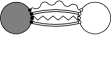
Figure 7: Free correlator of BMN operators. The first diagram on the top line is the sphere of $\langle\bar{\cal O}^{J}_{12,n}{\cal O}^{J}_{12,m}\rangle$, the middle two are $\langle\bar{\cal O}^{J}_{12,n}{\cal T}^{J,r}_{12,m}\rangle$ and the last one is $\langle\bar{\cal O}^{J}_{12,n}{\cal T}^{J,r}_{12}\rangle$. The diagrams on the bottom line are the torus of $\langle\bar{\cal O}^{J}_{12,n}{\cal O}^{J}_{12,m}\rangle$ on a periodic square.

We represent the traces of an operator by circles, the empty circles are composed mostly of $Z$s, the shaded ones mostly of $\bar{Z}$s. In the free theory the fields in the traces are connected by lines. Plain lines connect $Z$s to $\bar{Z}$s, wiggly or zigzag lines connect two impurities $\phi_{1}$ or $\phi_{2}$, respectively. The majority of lines are plain lines and on surfaces of low genus most of these lines run parallel to another. To make the diagrams more concise we draw a bunch of parallel plain lines (see fig. 1) as one double line. The number of constituent lines will be denoted by $a_{k}$ where $k$ is the label of the double line determined as follows: We consider the leftmost circle and label the double lines starting at the top in clockwise order from $1$ to the number of double lines. The value of a diagram is the sum over all possible sizes $a_{k}$ of double lines weighted with the phase factors of the BMN operators. For each circle the total number of lines must equal the number of fields on the trace, this is achieved by inserting a Kronecker delta into the sum. Furthermore, for an operator with two impurities, charge $J$ and mode number $n$ we insert the phase $\exp(2\pi ibn/J)$, where $b$ is the distance from the wiggly to the zigzag line in clockwise direction. Finally, we have to multiply by the normalization factors from the definition of the operators eqs.(3.9),(3.10). For example the third torus diagram in fig. 7 has the value

$$\frac{1}{J}\sum_{a_{1},\ldots,a_{6}=1}^{J}\delta_{a_{1}+\ldots+a_{6},J}\,\exp\frac{2\pi in(a_{2}+a_{3})}{J}\,\exp\frac{2\pi im(a_{1}+a_{4})}{J}.$$ (D.1)

This expression has the correct leading $J$ behavior, we can therefore transform the sum into an integral

$$\frac{1}{J}\int_{0}^{J}d^{6}a\,\delta(a_{1}+\ldots+a_{6}-J)\,\exp\frac{2\pi in(a_{2}+a_{3})}{J}\,\exp\frac{2\pi im(a_{1}+a_{4})}{J},$$ (D.2)

as we are not interested in $\mathcal{O}(1/J)$ corrections in this work. It turns out that for all relevant diagrams the corresponding sums can be approximated by integrals in the BMN limit. All diagrams that contribute to the correlators in eqs.(3.8),(3.14),(LABEL:double-single) are shown in fig. 7.

Radiative Corrections.

$+$ $-$ $-$ $+$

Figure 8: F-term interactions in $\langle\bar{\cal O}^{J}_{12,n}{\cal O}^{J}_{12,m}\rangle$ on the sphere. Another four diagrams have the two impurities interchanged.

The radiative corrections to the correlators are obtained by inserting the effective vertex eq.(C.14) into the matrix model correlator. The F-terms couple anti-symmetrically to an operator while the K-terms couple only to SO(6) traces. Only the singlet BMN operator has an SO(6) trace and the extra contributions will be calculated later. For the time being we would like to concentrate on the F-term. The relevant part of the $F$-term effective vertex is $(-g_{\scriptscriptstyle\mathrm{YM}}^{2}L/8\pi^{2})\mathop{\mathrm{Tr}}[\bar{Z}^{+},\phi_{i}^{+}][Z^{-},\phi_{i}^{-}]$. The trace can be separated into two traces linked by a line $\mathop{\mathrm{Tr}}[\bar{Z}^{+},\phi_{i}^{+}]T^{a}\,\mathop{\mathrm{Tr}}[Z^{-},\phi_{i}^{-}]T^{a}$. Graphically we thus represent the four-point scalar interactions by two three-point interactions joined by a dashed line. We will suppress the factor $(-g_{\scriptscriptstyle\mathrm{YM}}^{2}L/8\pi^{2})$ at intermediate stages and put it back in the end.

First of all, we will consider the sphere of the correlator of two BMN operators, $\langle\bar{\cal O}^{J}_{12,n}{\cal O}^{J}_{12,m}\rangle$, see fig. 8. In the first two diagrams the distance between the wiggly and zigzag line is $a_{1}$ and $a_{1}+1$, respectively. Furthermore, the two diagrams receive different signs from the effective vertex, a plus for the first, a minus for the second. Therefore the sum of both diagrams receives the effective phase factor

$$\exp\frac{2\pi ia_{1}n}{J}-\exp\frac{2\pi i(a_{1}+1)n}{J}=-2i\exp\frac{2\pi i(a_{1}+{\textstyle\frac{1}{2}})n}{J}\,\sin\frac{\pi n}{J}$$ (D.3)

from the left operator with mode number $n$. In the BMN limit this simplifies to

$$-\frac{2\pi in}{J}\exp\frac{2\pi ia_{1}n}{J}.$$ (D.4)

This can be generalised: When adjacent plain and zigzag lines connect a BMN operator with mode number $n$ and charge $J$ to an F-term vertex, the sum of the two possible contributions is $-2\pi in/J$ times the contribution where the zigzag line comes first in clockwise order. For the interactions between plain and wiggly lines the factor is $+2\pi in/J$. The sum of the four depicted diagrams is thus $(-2\pi in/J)(-2\pi im/J)$ times the free result. Together with the four diagrams where the wiggly line interacts and the prefactor $(-g_{\scriptscriptstyle\mathrm{YM}}^{2}L/8\pi^{2})$ the total one-loop result is $\lambda^{\prime}Lnm$ times the free result.

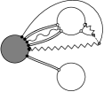
Figure 9: F-term interactions in correlators of BMN operators. The first three belong to the correlator $\langle\bar{\cal O}^{J}_{12,n}{\cal T}^{J,r}_{12,m}\rangle$, the next one to $\langle\bar{\cal O}^{J}_{12,n}{\cal T}^{J,r}_{12}\rangle$ and the last three to the torus of $\langle\bar{\cal O}^{J}_{12,n}{\cal O}^{J}_{12,m}\rangle$ on a periodic square.

Fig. 9 contains the diagrams that contribute to the remaining correlators in eqs.(3.8),(3.14),(LABEL:double-single). We have shown only representative diagrams, there are several other diagrams with different positions of the impurities and different orientations of inserted vertices. The first depicted diagrams on both lines contribute $\lambda^{\prime}Lnm$ times the free result of the corresponding correlator for the same reason as before. The other diagrams can also be shown to be proportional to the free result except the last one on the torus. As an example we will write down the phase factor from this particular diagram in the case $n=m$

$$-\exp\frac{2\pi i(a_{2}+a_{3})n}{J}\,\exp\frac{2\pi i(a_{1}+a_{3}+a_{4})n}{J}$$ (D.5)

where the two phases can be combined to $2\pi a_{3}n/J$. Adding the three diagrams where the zigzag line is interchanged with the plain lines on the interaction we get

$$-\exp\frac{2\pi ia_{3}n}{J}\left|1-\exp\frac{2\pi ia_{4}n}{J}\right|^{2}.$$ (D.6)

Then we add the cases where the wiggly line sits on one of the other two edges formed by double lines

$$-\left|1-\exp\frac{2\pi i(a_{3}+a_{4})n}{J}\right|^{2}-\exp\frac{-2\pi ia_{1}n}{J}\left|1-\exp\frac{2\pi ia_{4}n}{J}\right|^{2}.$$ (D.7)

This we must multiply by $2$ for interchange of impurities, the prefactor $(-g_{\scriptscriptstyle\mathrm{YM}}^{2}L/8\pi^{2})$ and the normalization $1/J$. After integration over the $a_{k}$ we get

$$\frac{g_{2}^{2}\lambda^{\prime}L}{8\pi^{2}}\left(\frac{2}{3}+\frac{5}{\pi^{2}n^{2}}\right)=\frac{g_{2}^{2}\lambda^{\prime}L}{8\pi^{2}}\mathcal{D}^{1}_{nn}.$$ (D.8)

Singlet Operators and K-term Interactions.

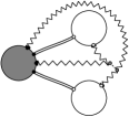
Figure 10: K-term interactions of singlet BMN operators. They contribute to $\langle\bar{\cal O}^{J}_{{\mathbf{1}},n}{\cal T}^{J,r}_{{\mathbf{1}},m}\rangle$, $\langle\bar{\cal O}^{J}_{{\mathbf{1}},n}{\cal T}^{J,r}_{{\mathbf{1}}}\rangle$ and the torus of $\langle\bar{\cal O}^{J}_{{\mathbf{1}},n}{\cal O}^{J}_{{\mathbf{1}},m}\rangle$.

For the singlet operator ${\cal O}^{J}_{{\mathbf{1}},n}$ there are additional contributions at one-loop due to the K-term interaction which couples to SO(6) traces. Assume the distance between the $\phi_{k}$ is $b$. Then the associated phase factor is $4\cos 2\pi inb/J$ explained as follows: The definition of the singlet operator involves a factor of ${\textstyle\frac{1}{2}}$. There is a contribution from each of the $4$ scalar flavors. Furthermore, there is no distinction between the two impurities and we must add up two conjugate complex phases giving a $2\cos$. Our definition of the singlet operator, however, involves also the piece $-\mathop{\mathrm{Tr}}\bar{Z}Z^{J+1}$ (a line between $\bar{Z}$ and $Z$ in the opposite direction is drawn as a curly line). The strength of this contribution was adjusted to add $-4$ to the above phase factor which gives the total effective phase factor

$$-4+4\cos\frac{2\pi inb}{J}=-8\sin^{2}\frac{\pi nb}{J}.$$ (D.9)

This immediately shows that there is no interaction for nearby impurities, $b=0$, due to the K-term and this reduces the number of contributing diagrams.

The only contributions to the correlators under consideration are due to the diagrams in fig. 10. Let us consider the first diagram. There is a phase factor of $-8\sin^{2}\pi nb/J$ from the coupling to $\bar{\cal O}^{J}_{{\mathbf{1}},n}$. The vertex couples to ${\cal T}^{J,r}_{{\mathbf{1}},m}$ only with $\bar{Z}$ and $Z$ which gives a factor of $-4$. Then, there is a crossed diagram with a different orientation of the dashed line which gives the same contribution. Finally this needs to be multiplied by the effective vertex prefactor $(-g_{\scriptscriptstyle\mathrm{YM}}^{2}L/32\pi^{2})$ and the total prefactor is $-16\lambda^{\prime}L/8\pi^{2}$ as in eqs.(3.25). The prefactor for the second diagram is the same, except that the effective vertex couples to the two $\phi_{k}$ of ${\cal T}^{J,r}_{{\mathbf{1}}}$ instead of $Z$ and $\bar{Z}$ of ${\cal T}^{J,r}_{{\mathbf{1}},m}$ and this amounts to a relative sign.

Appendix E Matrix elements

The matrix elements that appear in the computation of correlators. $M^{1}_{mn}$ and $\mathcal{D}^{1}_{mn}$ were already calculated in [8, 10]. Assume $|m|\neq|n|$, $m\neq 0$, $n\neq 0$.

$$M^{1}_{nn}\mathrel{} = \mathrel{}\frac{1}{60}-\frac{1}{24\pi^{2}n^{2}}+\frac{7}{16\pi^{4}n^{4}}$$

$$M^{1}_{n,-n}\mathrel{} = \mathrel{}\frac{1}{48\pi^{2}n^{2}}+\frac{35}{128\pi^{4}n^{4}}$$

$$M^{1}_{mn}\mathrel{} = \mathrel{}\frac{1}{12\pi^{2}(n-m)^{2}}-\frac{1}{8\pi^{4}(n-m)^{4}}$$

$$\mathord{}+\frac{1}{4\pi^{4}m^{2}n^{2}}+\frac{1}{8\pi^{4}mn(n-m)^{2}}$$

$$M^{2}_{nn}\mathrel{} = \mathrel{}-\frac{1}{40}+\frac{1}{12\pi^{2}n^{2}}-\frac{49}{128\pi^{4}n^{4}}$$

$$M^{2}_{n,-n}\mathrel{} = \mathrel{}-\frac{1}{96\pi^{2}n^{2}}-\frac{35}{256\pi^{4}n^{4}}$$

$$M^{2}_{mn}\mathrel{} = \mathrel{}-\frac{1}{8\pi^{2}(m-n)^{2}}+\frac{3}{16\pi^{4}(m-n)^{4}}+\frac{1}{8\pi^{4}(m+n)^{2}(m-n)^{2}}$$

$$\mathord{}-\frac{3}{16\pi^{4}m^{2}n^{2}}-\frac{3}{16\pi^{4}mn(m-n)^{2}}$$

$$\mathcal{D}^{1}_{nn}=\mathcal{D}^{1}_{n,-n}\mathrel{} = \mathrel{}\displaystyle\frac{2}{3}+\frac{5}{\pi^{2}n^{2}}$$

$$\mathcal{D}^{1}_{mn}\mathrel{} = \mathrel{}\frac{2}{3}+\frac{2}{\pi^{2}m^{2}}+\frac{2}{\pi^{2}n^{2}}$$

$$\mathcal{D}^{2}_{nn}=\mathcal{D}^{2}_{n,-n}\mathrel{} = \mathrel{}\displaystyle-\frac{1}{2}-\frac{45}{16\pi^{2}n^{2}}$$

$$\mathcal{D}^{2}_{mn}\mathrel{} = \mathrel{}-1-\frac{3}{2\pi^{2}n^{2}}-\frac{3}{2\pi^{2}m^{2}}+\frac{3}{4\pi^{2}(n-m)^{2}}+\frac{3}{4\pi^{2}(n+m)^{2}}$$

References

- [1] D. Berenstein, J. M. Maldacena and H. Nastase, “Strings in flat space and pp waves from 4 Super Yang Mills”, JHEP 04 (2002) 013, hep-th/0202021.
- [2] D. J. Gross, A. Mikhailov and R. Roiban, “Operators with large R charge in 4 Yang-Mills theory”, Annals Phys. 301 (2002) 31, hep-th/0205066.
- [3] A. Santambrogio and D. Zanon, “Exact anomalous dimensions of 4 Yang-Mills operators with large R charge”, Phys. Lett. B545 (2002) 425, hep-th/0206079.
- [4] C.-S. Chu, V. V. Khoze and G. Travaglini, “Three-point functions in 4 Yang-Mills theory and pp-waves”, JHEP 06 (2002) 011, hep-th/0206005.
- [5] M. Blau, J. Figueroa-O’Farrill, C. Hull and G. Papadopoulos, “Penrose limits and maximal supersymmetry”, Class. Quant. Grav. 19 (2002) L87, hep-th/0201081.
- [6] R. R. Metsaev, “Type IIB Green-Schwarz superstring in plane wave Ramond-Ramond background”, Nucl. Phys. B625 (2002) 70, hep-th/0112044.
- [7] R. R. Metsaev and A. A. Tseytlin, “Exactly solvable model of superstring in plane wave Ramond-Ramond background”, Phys. Rev. D65 (2002) 126004, hep-th/0202109.
- [8] C. Kristjansen, J. Plefka, G. W. Semenoff and M. Staudacher, “A new double-scaling limit of 4 super Yang-Mills theory and PP-wave strings”, Nucl. Phys. B643 (2002) 3, hep-th/0205033.
- [9] D. Berenstein and H. Nastase, “On lightcone string field theory from super Yang-Mills and holography”, hep-th/0205048.
- [10] N. R. Constable, D. Z. Freedman, M. Headrick, S. Minwalla, L. Motl, A. Postnikov and W. Skiba, “PP-wave string interactions from perturbative Yang-Mills theory”, JHEP 07 (2002) 017, hep-th/0205089.
- [11] H. Verlinde, “Bits, matrices and 1/N”, hep-th/0206059.
- [12] M. Spradlin and A. Volovich, “Superstring interactions in a pp-wave background”, Phys. Rev. D66 (2002) 086004, hep-th/0204146.
- [13] R. Gopakumar, “String interactions in pp-waves”, hep-th/0205174.
- [14] Y. Kiem, Y. Kim, S. Lee and J. Park, “PP-wave/Yang-Mills correspondence: An explicit check”, Nucl. Phys. B642 (2002) 389, hep-th/0205279.
- [15] M.-X. Huang, “Three point functions of 4 Super Yang Mills from light cone string field theory in pp-wave”, Phys. Lett. B542 (2002) 255, hep-th/0205311.
- [16] P. Lee, S. Moriyama and J. Park, “Cubic interactions in pp-wave light cone string field theory”, Phys. Rev. D66 (2002) 085021, hep-th/0206065.
- [17] M. Spradlin and A. Volovich, “Superstring interactions in a pp-wave background. II”, hep-th/0206073.
- [18] I. R. Klebanov, M. Spradlin and A. Volovich, “New effects in gauge theory from pp-wave superstrings”, Phys. Lett. B548 (2002) 111, hep-th/0206221.
- [19] M.-X. Huang, “String interactions in pp-wave from 4 Super Yang Mills”, Phys. Rev. D66 (2002) 105002, hep-th/0206248.
- [20] U. Gürsoy, “Vector operators in the BMN correspondence”, hep-th/0208041.
- [21] C.-S. Chu, V. V. Khoze, M. Petrini, R. Russo and A. Tanzini, “A note on string interaction on the pp-wave background”, hep-th/0208148.
- [22] M. Bianchi, B. Eden, G. Rossi and Y. S. Stanev, “On operator mixing in 4 SYM”, Nucl. Phys. B646 (2002) 69, hep-th/0205321.
- [23] G. Arutyunov and E. Sokatchev, “Conformal fields in the pp-wave limit”, JHEP 08 (2002) 014, hep-th/0205270.
- [24] C.-S. Chu, V. V. Khoze and G. Travaglini, “pp-wave string interactions from n-point correlators of BMN operators”, JHEP 09 (2002) 054, hep-th/0206167.
- [25] A. Parnachev and A. V. Ryzhov, “Strings in the near plane wave background and AdS/CFT”, JHEP 10 (2002) 066, hep-th/0208010.
- [26] G. Arutyunov, S. Penati, A. C. Petkou, A. Santambrogio and E. Sokatchev, “Non-protected operators in 4 SYM and multiparticle states of AdS(5) SUGRA”, Nucl. Phys. B643 (2002) 49, hep-th/0206020.
- [27] F. Gonzalez-Rey, I. Y. Park and K. Schalm, “A note on four-point functions of conformal operators in 4 Super-Yang-Mills”, Phys. Lett. B448 (1999) 37, hep-th/9811155.
- [28] B. Eden, P. S. Howe, C. Schubert, E. Sokatchev and P. C. West, “Four-point functions in 4 supersymmetric Yang-Mills theory at two loops”, Nucl. Phys. B557 (1999) 355, hep-th/9811172.
- [29] B. Eden, P. S. Howe, C. Schubert, E. Sokatchev and P. C. West, “Simplifications of four-point functions in 4 supersymmetric Yang-Mills theory at two loops”, Phys. Lett. B466 (1999) 20, hep-th/9906051.
- [30] M. Bianchi, S. Kovacs, G. Rossi and Y. S. Stanev, “On the logarithmic behavior in 4 SYM theory”, JHEP 08 (1999) 020, hep-th/9906188.
- [31] N. I. Ussyukina and A. I. Davydychev, “An approach to the evaluation of three and four point ladder diagrams”, Phys. Lett. B298 (1993) 363.
- [32] E. D’Hoker, D. Z. Freedman, S. D. Mathur, A. Matusis and L. Rastelli, “Extremal correlators in the AdS/CFT correspondence”, hep-th/9908160.
- [33] J. Ginibre, “Statistical ensembles of complex, quaternion and real matrices”, J. Math. Phys. 6 (1965) 440, see also [37].
- [34] K. Okuyama, “4 SYM on and pp-wave”, hep-th/0207067.
- [35] I. K. Kostov and M. Staudacher, “Two-dimensional chiral matrix models and string theories”, Phys. Lett. B394 (1997) 75, hep-th/9611011.
- [36] I. K. Kostov, M. Staudacher and T. Wynter, “Complex matrix models and statistics of branched coverings of 2D surfaces”, Commun. Math. Phys. 191 (1998) 283, hep-th/9703189.
- [37] M. L. Mehta, “Random matrices”, second edition, Academic Press, 1990.