Lab/UFR-HEP/0209
NC Effective Gauge Model for
Multilayer FQH States

Abstract

We develop an effective field model for describing FQH states with rational filling factors that are not of Laughlin type. These kinds of systems, which concern single layer hierarchical states and multilayer ones, were observed experimentally; but have not yet a satisfactory non commutative effective field description like in the case of Susskind model. Using $D$ brane analysis and fiber bundle techniques, we first classify such states in terms of representations characterized, amongst others, by the filling factor of the layers; but also by proper subgroups of the underlying $U\left(n\right)$ gauge symmetry. Multilayer states in the lowest Landau level are interpreted in terms of systems of $D2$ branes; but hierarchical ones are realized as Fiber bundles on $D2$ which we construct explicitly. In this picture, Jain and Haldane series are recovered as special cases and have a remarkable interpretation in terms of Fiber bundles with specific intersection matrices. We also derive the general NC commutative effective field and matrix models for FQH states, extending Susskind theory, and give the general expression of the rational filling factors as well as their non abelian gauge symmetries.

Keywords   : Multilayer and FQH hierarchies; Branes and fiber bundles on branes, NC non abelian Chern Simons gauge theory, Matrix model

1 Introduction

Susskind proposal [1] that Non-Commutative (NC) Chern-Simons gauge theory on the $(2+1)$ space provides a natural framework to study the Laughlin state of filling factor $\nu_{L}=\frac{1}{k}$, $k$ a positive odd integer. This proposal  has opened a new way to deal with the effective field models of Fractional Quantum Hall (FQH) fluids and offered possible interpretations in terms of $D$ brane solitons of type $II$ superstring theory [2, 3, 4]. Since this important development, an intensive interest has been given to explore further this remarkable issue and several basic results has been derived. A regularized version of the Susskind NC effective field theory using finite dimensional matrix model techniques has been introduced in [5] to study FQH droplets. There, it has been shown that consistency requires  the introduction of an extra field, the polychronakos field, which is a regulator field playing an important role at the quantum level [6, 8]. Along with these developments, it has been also conjectured that a specific assembly of a system of $D0$, $D2$ and $D6$ branes and $F1$ strings, stretching between $D2$ and $D6$, has a low energy dynamics similar to the fundamental state of FQH systems [9, 10]. For other applications and issues see [11, 12].

In Susskind NC model, the non commutativity parameter $\theta$ of the co-moving plane coordinates is related to the filling factor $\nu_{L}$ and then to the Chern-Simon effective field coupling $\lambda_{CS}$ as $\theta\mathcal{B}_{ex}\nu_{L}=\nu_{L}\lambda_{CS}=1$; where $\mathcal{B}_{ex}$ is the external magnetic field. This relation, which get quantum corrections, shifting the level $k$ of the CS gauge theory [6, 7, 13], has been used in [14, 15, 16] to approach a specific class of states that are not of Laughlin kind; that is FQH states with rational values type $\nu_{2}^{\left(h\right)}=\frac{k_{1}+k_{2}}{k_{1}k_{2}}$ with $k_{1}$and $k_{2}$ positive odd integers. These kinds of states, which are just the leading elements of general ones having the filling factor taking general rational values, belong to two kinds of FQH systems: (1) multilayer FQH systems in the ground state and beyond and (2) generic levels of the so called hierarchical series.

Like for the Laughlin ground state, FQH states with general rational values of the filling factor, such as, the well known $\frac{2}{5}$, $\frac{2}{3}$,$\frac{3}{7}$,…; were observed experimentally several years ago; but are not covered by the Susskind NC theory which, due to quantization and unitarity conditions, requires that $1/\nu$ should be positive integer.

In [14], see also [15, 16], an extension of Susskind NC field model to cover hierarchical states has been approached by noting that some FQH hierarchical states, at given levels $n$, can be usually decomposed as a particular sum over $n$ Laughlin states built in a recurrent manner. In Haldane hierarchy, this splitting feature was first noted on the leading elements of the series such as $\frac{2}{5}$ and $\frac{3}{7}$, which have the remarkable decomposition

$$\frac{2}{5} = \frac{1}{3}+\frac{1}{15},$$

$$\frac{3}{7} = \frac{1}{3}+\frac{1}{15}+\frac{1}{35},$$ (1.1)

allowing to interpret them as bounds of Laughlin states. Here we will show that this splitting is in fact valid at any level $n$ and follows due to a remarkable exact mathematical result of the continuous fraction $\left[p_{1}...p_{n}\right]$; which ensures that the level $n$ of Haldane series $\nu_{n}^{\left(Hal\right)}$ can be usually brought to the form

$$\mathrm{\nu}_{n}^{\left(Hal\right)}=\frac{1}{k_{1}}+\frac{1}{k_{2}}+...+\frac{1}{k_{n}},$$ (1.2)

where $k_{i}$ are some specific odd integers to be computed explicitly in section 5. Similarly, Jain hierarchical series may, roughly speaking, be also thought of as given by the special decomposition,

$$\mathrm{\nu}_{n}^{\left(Jain\right)}=\frac{1}{2np\pm 1}+\frac{1}{2np\pm 1}+...+\frac{1}{2np\pm 1}.$$ (1.3)

Analogous analysis may be written down as well for this sequence; for details see section 5 eqs(5.13-17). What interest us from this brief presentation is note that in both decompositions (1.1-.2) and (1.3), one sees that the level $n$ of hierarchy is also the number of filled lowest Landau levels, (LL${}_{1},...,$LL_n for short) and moreover each LL_i behaves as a kind of Laughlin state with filling factor $1/k_{i}$; $k_{i}$ odd integer.

Despite these partial results and others established in recent literature [15, 16, 17, 18, 19, 20], there are however basic questions, regarding states with rational filling factors, that remain without convincing answers. Besides the non commutative non abelian $U\left(n\right)$ Chern Simons gauge model describing multilayer states with filling factors

$$\mathrm{\nu}_{U\left(n\right)}=n/k,$$ (1.4)

where $k$ is the level of the Chern Simons model, no consistent NC field theoretical construction extending Susskind NC model has been obtained neither for hierarchical states, nor for multilayer systems. To this lack, one should also add an other notable one concerning the classification of FQH states with rational value. For example, if one considers state with $\mathrm{\nu}=2/5$ and try to list all possible FQH systems in which it can appear, one sees that there is a variety of possibilities: To write down this list, note first of all that such states may appear into two kinds of system: (1) multilayer system and (2) single layer hierarchical states, offering by the occasion the first ingredient in the classification.

Multilayer states

If one focuses on the state $\mathrm{\nu}=2/5$ and considers that the two layers $\mathcal{L}_{1}$ and $\mathcal{L}_{2}$ of the system are taken in the ground state; then we have the following natural representations:

(a) The state $\mathrm{\nu}=2/5$ realized as an irreducible representation; like in NC non abelian $U\left(2\right)$ Chern Simons gauge model with a level $k=5$. Here, the two layers $\mathcal{L}_{1}$ and $\mathcal{L}_{2}$ should be completely symmetric.

(b) As a reducible state $1/5+1/5$ like in uncoupled NC abelian $U\left(1\right)\times U\left(1\right)$ Chern Simons model with equal levels $k_{1}=k_{2}=5$. This model is expected to be obtained from the previous representation after breaking of the $U\left(2\right)$ gauge symmetry and integrating out massive modes.

(c) As a reducible state $1/3+1/15$ like in uncoupled NC abelian $U\left(1\right)\times U\left(1\right)$ Chern Simons model with different levels; i.e $k_{1}=3$ and $k_{2}=15$. Here the quantum properties of the two layers $\mathcal{L}_{1}$ and $\mathcal{L}_{2}$ are different and this representation seems to have nothing to do with the original NC non abelian $U\left(2\right)$ Chern Simons model. One expects then to get multilayer effective field realizations other than the NC non abelian Chern Simon gauge model. We will show later on, that at level $n=2$ for instance, a possible generalization $\mathrm{\nu}_{U\left(1\right)^{2}}$ of eq(1.4) is,

$$\mathrm{\nu}_{U\left(1\right)^{2}}=\frac{k_{1}+k_{2}}{k_{1}k_{2}-l^{2}}$$ (1.5)

For $k_{1}\neq k_{2}$, this equation corresponds to the $U\left(1\right)^{2}$ model describing two parallel layers with different individual filling factors; $1/k_{1}$and $1/k_{2}$, with $k_{1}$ and $k_{2}$ odd integers. Interactions between layers shift the inverse of the free filling factor by the amount $l^{2}/k_{1}k_{2}$. Moreover, this relation allows to recover the Jain sequence, which is obtained from (1.5), by looking for integer solutions of the following eq

$$l=\frac{1}{2}\sqrt{\left[2k_{1}-\left(4p+1\right)\right]\left[2k_{2}-\left(4p+1\right)\right]-\left(4p+1\right)^{2}};\quad l\in Z^{+}$$ (1.6)

where the integer $p$ is as in eq(1.3). The formula (1.5) we have given above is in fact the second simplest example of a more general result to be established in subsection 3.1, eq(3.46); expressing the filling fraction $\mathrm{\nu=Tr}\left[\mathrm{\kappa}^{-1}\right]$ of multilayer FQH states in terms of the inverse of a hermitian matrix $\mathrm{\kappa}$ of $GL\left(n;\mathbf{Z}^{+}\right)$ with odd integer diagonal terms. It permits to recover all possible picture including the non abelian model which correspond to the solutions of the constraint eq $U\mathrm{\kappa=\kappa}U$, where $U$ is are $n\times n$ matrix describing the gauge transformations.

Single Layer hierarchical states

In the case of a single layer $\mathcal{L}$ and considering usually the state $\mathrm{\nu}=2/5$, one may also write down a list of possible realizations;

(d) The state $\mathrm{\nu}=2/5$ realized as an irreducible representation $2/5$, like in the Lopez and Fradkin model [21],

(e) As a reducible state $1/5+1/5$ like in Jain series eq(1.3),

(f) As a reducible state $1/3+1/15$ like Haldane series decomposition (1.1-2).

In addition to these list of representations, one should also add those hierarchical states with rational values of filling factors living on multilayer systems; that is systems with several layers taken outside the ground state.

In this paper, we present a unified effective field model for studying FQH states with rational filling fraction that come either from multilayer systems, hierarchical states of a single layer or again hierarchical states in multilayer systems. Our way of doing is mainly motivated by similarities between FQH liquids and $D$ brane systems of type $II$ string theory [22]. Using these tools and others geometric ones, we develop a general effective field model for FQH states with rational filling factors. More precisely, we use ideas borrowed from $D$ brane physics [23] and fiber bundles, F$\left(\cup D2\right)$ on a set of $D2$ branes, to study FQH liquids with rational filling factors. As a result, we obtain the general NC effective field and matrix theories modeling FQH states with generic rational filling factors. The generating functional action of our effective field model, which has different sectors, reads formally, as

$$\mathcal{Z}\left[A\right]=\int\prod_{\text{{\small massive fields}}}\mathcal{D}\left[A\right]\exp-i\left(\int d^{3}y\sum_{\mathcal{L}_{a}}\sum_{{LL}_{i_{a}}}\mathrm{L}\left(A\right)\right),$$ (1.7)

where $\left\{\cup_{a=1}^{n}\mathcal{L}_{a}\right\}$ stands for a system of $n$ layers $\mathcal{L}_{a}$ interpreted as a set of  n parallel $D2$ branes, and where $\left\{\cup_{i_{a}=1}^{m_{a}}{LL}_{i_{a}}\right\}$ is the set of the $m_{a}$ filled lowest Landau level associated with the $a-th$ layer $\mathcal{L}_{a}$. In this relation, $\mathrm{L}\left(A\right)$ is a lagrangian density which reads, for $U\left(n\right)$ gauge invariant model, as in eq(7.6-7) and, in the case $n=1$ and $m_{1}=1$, reduces to the well known Susskind NC field model for Laughlin state. This functional action exhibits, amongst others, the following features.

• Extends, to multilayer states and hierarchical ones, the original Susskind NC field theory and the Susskind-Polychronakos regularized matrix model initially obtained for the case of a single layer in the ground state. Our model is general; it contains as well the single layer states belonging to Jain and Haldane series as particular ones.

• Answers remarks made in [21], regarding consistency of Wen-Zee ( WZ) model for hierarchy [29, 30, 31]; in particular the point concerning the stability of the WZ conserved currents. Though, we support the arguments given in [21], we give nevertheless validity conditions under which WZ effective field approach works. We also work out explicitly the NC field and matrix models generalizing such ideas.

• Presents a framework where single layer hierarchical states with rational filling factors and the ground configuration of multilayers as well as multilayer hierarchical states are treated in a unified way, in perfect agreement with Susskind basic idea [1] and non abelian symmetries of parallel branes.

The presentation of this paper is as follows: In section 2, we describe, in two subsections, FQH states with rational filling factors, belonging to multilayer systems on one hand and on the other hand to a single layer hierarchical states. The multilayer system is viewed as represented by $n$ parallel $D2$ branes located at the positions $y^{3}=d_{a}$, in the direction of the external magnetic field $\mathcal{B}_{ex}$. The single layer hierarchical states are interpreted as fiber bundles on $D2$ branes. Here also, we fix some terminology and convention notations. In section 3, we study commutative effective field models for multilayer states in the lowest Landau levels. We distinguish between several gauge fields models with abelian and non abelian gauge symmetries. In this regards, we show that only layers with same filling factor; say $k_{1}=k_{2}=...=k_{n}=k$; which can lead to a $U\left(n\right)$ non abelian symmetry; otherwise the $U\left(n\right)$ symmetry is broken down to subgroups depending on the number of equal $k_{a}$’s one has. In case where all $k_{i}$’s are different, the effective $U\left(1\right)^{n}$ abelian gauge field models we obtain are of two types: (i) either without interactions; i.e $k_{ab}=0$ for $a\neq b$, and then the total filling factor is given by the sum of the individual filling factors or (ii) having interactions; i.e $k_{ab}\neq 0$ for $a\neq b$, as in Wen-Zee theory for single layer hierarchical states. In this case, the filling factor have a general form given by eq(3.46), which contain Haldane and Jain series as special cases. We also use this occasion to give a classification of the various type of the generalizations of Laughlin wave functions one encounters in FQH literature and take the opportunity to complete some partial results in this matter. In section 4, we study the NC non abelian effective gauge field and matrix models for multilayers states where the usual NC non abelian $U\left(n\right)$ Chern Simons gauge theory appears as just the most symmetric representation. The other less symmetric representations are also studied. In section 5, we study the Wen-Zee effective field theory for single layer states with rational filling factors and review some aspects regarding Jain and Haldane hierarchies, which are now viewed as two special fiber bundles whose explicit realizations are given in subsections 5.2 and 5.3. In section 6, we give the NC gauge fields and matrix models for single layer hierarchical states and in section 7, we give a discussion concerning hierarchy in multilayer systems and make a conclusion..

2 FQH Hierarchies and Mutilayer Systems

Experiments on Hall systems showed the existence of stable states at critical values of filling factor $\nu$ taking in general rational values; the familiar $\mathrm{\nu}=\frac{1}{3},$ $\frac{2}{5}$, $\frac{3}{7}$ are examples amongst many others. Laughlin constructed an explicit trial wave function to explain QH state partially filled with $\mathrm{\nu}=\frac{1}{m}$ where $m$ odd integer. He argued that the elementary excitations from the stable states are quasiparticles with fractional electric charge $q=\pm\nu e$ and obey a generalized statistics. In this scheme, electrons are thought of as a kind of condensate of $m$ quasiparticles and occupy the lowest Landau level ( LLL ). Recently Susskind completed this model by showing that the right $\left(1+2\right)$ dimension effective field theory that describe Laughlin state is a NC Chern Simons $U\left(1\right)$ gauge model on Moyal surfaces.

To describe the states with general values of the filing factor; say of the form $\mathrm{\nu}=\frac{n}{p}$, there is no standard method to follow; but rather different approaches one can use to study such states. These ways have a common denominator; as all of them are based on the Laughlin model. Motivated by the recent developments [14, 15, 16] based on Susskind model; its regularized finite dimensional matrix formulation as well as results on hierarchical states using exact algebraic feature on the continuous fraction, we explore in this section the main representations of FQH systems that lead to rational values of the filling fraction. We also fix our terminology regarding the correspondence between layers and $D2$ branes, on one hand, and Landau levels and fiber bundles on the other hand.

2.1 Multilayer Representation

The multilayer FQH states with rational filling factors, we will be considering here are obtained from a system of $\mathcal{N}_{e}=\left(N_{1}+...+N_{n}\right)$ electrons moving in a set of $n$ parallel layers $\mathcal{L}_{a}$ in presence of an external  constant and orthogonal magnetic field $\mathcal{B}_{ex}$ with a constant flux $\int\mathcal{B}_{ex}=\mathcal{N}_{\phi}$. As a convention of notation, we will denote this system as,

$$\left\{n\mathcal{L}\equiv\cup_{a=1}^{n}\mathcal{L}_{a};\quad\mathcal{L}_{a}\|\mathcal{L}_{b}\right\}.$$ (2.1)

Note that parallelism of layers should be understood as a local condition. If we let $\left\{\mathcal{O}_{a}^{I};\quad I=1,2,...\right\}$ be topological basis of local open sets covering the $\mathcal{L}_{a}$ layers

$$\mathcal{L}_{a}=\cup_{I\geq 1}\mathcal{O}_{a}^{I};\quad\mathcal{O}_{a}^{I}\cap\mathcal{O}_{a}^{I}\neq\emptyset,$$

then $\mathcal{L}_{a}$ is said parallel to $\mathcal{L}_{b}$ should be thought of as an open set $\mathcal{O}_{a}^{I}$ of $\mathcal{L}_{a}$ is parallel to an open set $\mathcal{O}_{b}^{J}$ of $\mathcal{L}_{b}$. In this paper, we will simplify the presentation by focusing our analysis directly on layers. Moreover since the $N_{a}$ electrons on the layer $\mathcal{L}_{a}$ may be sitting in different Landau levels $\left\{{LL}_{i}\right\},$ we will add, when necessary, an extra index to implement this feature into the formalism. Thus $\mathcal{L}_{a}^{i_{a}}$ denote a FQH configuration of electrons in $i_{a}-th$ Landau levels of the layer $\mathcal{L}_{a}$. Later on, we will give a representation of this configuration in terms of a fiber bundle on $\mathcal{L}_{a}$; that is,

$$\mathcal{L}_{a}^{i_{a}}\equiv\left({LL}_{i_{a}}{;}\mathcal{L}_{a}\right)\equiv{F}_{i_{a}}\left(\mathcal{L}_{a}\right)$$ (2.2)

For the moment let us fix our attention on the lowest Landau level and suppose that all layers $\mathcal{L}_{a}$ of the system are of Laughlin type; i.e with filling factors $\nu_{a}=1/k_{a}$. Since the FQH ( patches of ) layers are mainly two dimensional real surfaces, it is natural to assimilate the $\left\{n\mathcal{L}\right\}$ system to an assembly of $n$ parallel $D2$ branes parameterized by the local ( patches ) coordinates

$$nD2 \sim \left\{y_{a}^{\mu}=\left(y^{1},y^{2},y^{3}=d_{a}\right);\quad a=1,...,n\right\};$$

$$\mathcal{B}_{ex} = \varepsilon^{3\alpha\beta}\text{ }\partial_{\alpha}\mathcal{A}_{\beta}\equiv\varepsilon^{30\alpha\beta}\text{ }\partial_{\alpha}\mathcal{A}_{\beta},$$ (2.3)

where $\left|d_{a}-d_{b}\right|$ is the distance separating the pair of layers $\left(\mathcal{L}_{a},\mathcal{L}_{b}\right)$, $\varepsilon^{3\alpha\beta}$ the completely three dimension antisymmetric tensor and where $\mathcal{A}_{\beta}$ is the external vector potential; see figure 1. Since electrons moving in this system have intra an inter layers interactions, one may use the $\left|d_{a}-d_{b}\right|$ layers inter-distances and D branes symmetries to classify the various possible models.

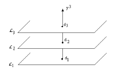
Figure 1: This figure represents a system of $n$ $\left(n=3\right)$ parallel layers $\left\{\mathcal{L}_{a}\right\}$ normal to the external magnetic field $\mathcal{B}_{ex}=\varepsilon^{3\mu\nu}\partial_{\mu}\mathcal{A}_{\nu}$.  These layers are represented by $n$ parallel $D2$ branes filling the plane $(y^{1},y^{2})$ located at the positions $y^{3}=d_{c};$ $c=1,...,n;$  with spacings $d_{ab}=d_{a}-d_{b}$. These layers may be either distant enough from each others as in  $U(1)^{n}$  gauge theory for instance or very close, eventually coincident. They may also have different filling factors.

According to the values of $\left|d_{a}-d_{b}\right|$, one can show that the number of configurations of $\left\{n\mathcal{L}\right\}$ is linked to the subgroups of the $U\left(n\right)$ symmetry. Two special configurations of the layers are those associated with the two following extreme cases: (i) the case where all $D2$ branes are distant enough from each others; i.e,

$$\left|d_{a}-d_{b}\right|>>>1,\quad\forall a,b=1,...,n.$$ (2.4)

In this situation, layers interactions carried by massive modes may be ignored and, roughly speaking, the underlying symmetry of the effective Chern Simons model describing the FQH multilayer system is $U\left(1\right)^{n}$. (ii) The other extreme case deals with the situation where all $D2$ branes coincide, ie

$$\left|d_{a}-d_{b}\right|<<<1,\quad\forall a,b=1,...,n.$$ (2.5)

This FQH configuration is described by an effective Chern Simons model with a non abelian $U\left(n\right)$ gauge invariance. The remaining situations correspond to the various systems with gauge invariances given by subgroups of $U\left(n\right)$.

2.2 Hierarchical Representation

We start by noting that there are two kinds of hierarchical FQH states; those involving several lowest Landau levels $\left\{\cup_{i=1}^{m}{LL}_{i}\right\}$ of a given single layer $\mathcal{L}$ in the sense of the decompositions eqs(1.1-3); and those implying various Landau levels $\left\{\cup_{a=1}^{n}\cup_{i_{a}=1}^{m_{a}}{LL}_{i_{a}}\right\}$ of a multilayer system $\left\{\cup_{a=1}^{n}\mathcal{L}_{a}\right\}$.  The second are naturally more general. Here we shall describe the first kind of states; but later on we shall give the general result.

2.2.1 Case of a single Layer

As we have said, FQH states with filling factor that are not of Laughlin type exist also for the case of one layer $\mathcal{L}$. This is the case for instance of the so called hierarchical states belonging to Jain and Haldane series. In the picture; one layer $\mathcal{L}$ $\longleftrightarrow$ one $D2$ brane,

$$\mathcal{L}\longleftrightarrow\mathcal{D}2,$$ (2.6)

where one has only one gauge field describing the displacement of the fluid, it seems a priori not obvious to describe such kind of states using Chern Simons $U\left(1\right)$ gauge field model as also noted in [21]. In this section we want to present two scenarios to overcome this difficulty. The first one is based on: (1) abandoning the correspondence; one layer $\mathcal{L}$ $\longleftrightarrow$ one $D2$ brane in profit of one Landau level ${LL}$ $\longleftrightarrow$ one $D2$ brane,

$${LL}\longleftrightarrow D2.$$ (2.7)

In this way of viewing things, the problem is solved since we have several gauge fields at hand and so the brane multilayer representation $\left\{\cup_{a=1}^{n}\mathcal{L}_{a}\right\}$ considered in subsection 2.1, translates completely to a multi Landau levels representation $\left\{\cup_{a=1}^{n}{LL}_{a}\right\}$.  The results one gets are quite similar to those one obtains for the multilayer system; it suffices to make the substitution

$$\mathcal{L}_{a}\rightarrow{LL}_{a}.$$ (2.8)

This idea has been used in [14] to study Haldane hierarchical states. We will skip the details here and goes to the second realization which interest us in this paper.

The second scenario, for studding single layer hierarchical states, at level $k$, is based on the physical idea that, instead of having only the first Landau level occupied like in Laughlin model; one can have as well other neighboring Landau levels occupied by electrons. This is mainly the content of the idea behind hierarchical models involving several kinds of quasi-particles like in Haldane case, eq(1.2); see figures 2.

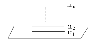
Figure 2: This figure illustrates a single layer $\mathcal{L}$  where the first $n$ Landau levels are occupied. We suppose that all levels are of Laughlin type as in the decompositions eqs(1.1-3). The way in which these Landau levels are occupied depends on the model one is considering. In general one may have different filling factors as in eq(1.2) and possible interactions between the various Levels.

This scheme may be also be interpreted as describing $k$ branches of FQH liquid as in the case of hydrodynamic droplets and edge excitations of systems with boundaries [21]. From the mathematical view, both of the bulk and edge levels can be implemented in terms of fiber bundles idea; see figures 3.

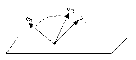
Figure 3: This figure represents a D2 brane and n dimensional fiber above a point on D2. Each direction $\alpha_{i},i=1,...,n;$  of this fiber is associated with the i-th Landau level of the FQH layer realized here by the D2 brane. From this view point, Laughlin model with filling factor $1/p$ is then associated with a one dimensional fiber bundle generated by the $\alpha_{1}$  vector with a norm equal to the odd integer p.

In the fiber bundle picture, one insists on having the correspondence (2.6); while the $i-th$ Landau Level ${LL}_{i}$ is thought of as a fiber Fⁱ above the $\mathcal{D}2$ brane which now plays the role of a base manifold $B$;

$$\left({LL}_{k};\mathcal{L}\right)\longleftrightarrow{F}^{k}\left({\large B}\right)\longleftrightarrow\left({V}_{k}{;}\mathcal{D}2\right),$$ (2.9)

where ${V}_{k}$ is a $k$ dimension vector space on the set of integers and is defined globally on the base. In this way, one has at hand various $U\left(1\right)$ gauge fields components $A_{\mu}^{i}\left(y\right)$; i.e,

$$A_{\mu}\left({LL}_{i};\mathcal{L}\right)\longleftrightarrow A_{\mu}^{i}\left(\mathcal{L}\right),$$ (2.10)

to describe the various $\left\{{LL}_{i}\right\}$ Landau levels. The effective field theory one expects is a Chern Simons gauge field model on the fiber bundle F$\left(B\right)$, which we want to build now.

The single layer $\mathcal{L}$, viewed now as a $\mathcal{D}2$ brane, has world volume parameterized by the $\left\{y=\left(y^{\mu}\right)\right\}$ coordinates. Fiber bundles ${F}\left(\mathcal{L}\right)$ based on $\mathcal{L}$ are generally given by the union of  fibers ${F}_{y}$ based on each point $y$ of the base.

$${F}\left(\mathcal{L}\right)=\cup_{y}{F}_{y}\left(\mathcal{L}\right)$$ (2.11)

Each fiber ${F}_{y}$ is a vector space parameterized by $\left(\alpha_{i};y\right)$, where $\alpha_{i}$ are some linearly independent vectors defining the vector basis of ${F}_{y}$. Since in our present case, the $\alpha_{i}$’s are $y$ independent, the fibers ${F}_{y}$ are the same every where on the base; this is why we shall drop the $y$ index on ${F}_{y}$ which now on will be denoted as ${V}\left(\mathcal{L}\right)$. Moreover since the level $k$ of the hierarchy can be any positive integer, ${V}\left(\mathcal{L}\right)$ should be a priori an infinite dimensional vector space which we endow with the orthonormal canonical basis.

$$\left\{\mathbf{e}_{i};\quad\mathbf{e}_{i}\cdot\mathbf{e}_{i}=\delta_{ij};\quad i,j\in\mathbf{Z}\right\}.$$ (2.12)

Though we will deal only with finite $m$ dimension proper subspaces ${V}_{m}\left(\mathcal{L}\right)$ of ${V}\left(\mathcal{L}\right)$ since generally one is interested to the few leading terms of the hierarchy; one can address the mathematical structure of ${V}\left(\mathcal{L}\right)$ in its general form. Problem induced by the infinite series one my encounters, such as the convergence of trace on infinite matrices for instance, may be regularized as in [25, 26]. Furthermore, as hierarchy at generic levels is described in a recurrent manner, namely

$$\text{level }1\subset\text{level }2\subset...\subset\text{level }\left(n-1\right)\subset\text{level }n\subset...$$ (2.13)

we demand that the proper subspaces ${V}_{n}\left(\mathcal{L}\right)$ of ${V}\left(\mathcal{L}\right)$ have to verify,

$${V}_{1}\left(\mathcal{L}\right)\subset{V}_{2}\left(\mathcal{L}\right)\subset...\subset{V}_{n}\left(\mathcal{L}\right)\subset...\subset{V}\left(\mathcal{L}\right).$$ (2.14)

Note that a generic proper subspace ${V}_{m}\left(\mathcal{L}\right)$ has a canonical basis induced from the mother space ${V}\left(\mathcal{L}\right)$. However, because of the physics we are looking to describe, we will introduce the special $\left\{\alpha_{i};1\leq i\leq m\right\}$ vectors basis of ${V}_{m}\left(\mathcal{L}\right)$ with the property of having non zero intersection matrix; that is the $\alpha_{i}$’s form a non orthogonal basis taken as,

$$\alpha_{i}\cdot\alpha_{j}=\mathrm{G}_{ij}$$ (2.15)

The matrix $\mathrm{G}_{ij}$ appearing in this relation is a hermitian and invertible $m\times m$ matrix; it will be interpreted as the matrix appearing in the Wen-Zee effective fields model [38, 39, 40, 41, 42, 43]. So we shall refer to this basis as Wen-Zee one and then to the fiber bundle as Wen-Zee fiber. We will also see later on, when we study NC effective field models for hierarchical states going beyond the NC Susskind model; that it is useful to extend the sequence (2.14) by introducing a one dimension bundle ${V}_{0}\left(\mathcal{L}\right)$ associated with the constant background appearing in the Susskind map that led to the discovery of NC Chern Simons model for Laughlin states. As such, we have

$${V}_{0}\left(\mathcal{L}\right)\subset{V}_{1}^{\prime}\left(\mathcal{L}\right)\subset{V}_{2}^{\prime}\left(\mathcal{L}\right)\subset...\subset{V}_{n}^{\prime}\left(\mathcal{L}\right)\subset...\subset{V}\left(\mathcal{L}\right),$$ (2.16)

where now ${V}_{m}^{\prime}\left(\mathcal{L}\right)$ have $\left(m+1\right)$ dimensions. The new vector basis is then $\left\{\alpha_{i};0\leq i\leq m\right\}$ and the previous $\mathrm{G}_{ij}$ intersection matrix now becomes a $\left(m+1\right)\times\left(m+1\right)$ matrix.

$$\mathrm{S}_{ij}=\left(\begin{array}[]{cc}\mathrm{G}_{00}&\mathrm{G}_{0j}\\ \mathrm{G}_{i0}&\mathrm{G}_{ij}\end{array}\right)$$ (2.17)

Besides the useful choice $\mathrm{S}_{00}=1$ we will make later, we require that this generalized matrix is hermitian and invertible as well.

2.2.2 Case of Multilayers

Hierarchical states of multilayer system are described by a general fiber bundle $\left({V};B\right)$ whose base B$=\left\{n\mathcal{D}2\right\}$ and fiber V$=\left\{\cup_{a=1}^{n}\cup_{i_{a}=1}^{m_{a}}{LL}_{i_{a}}\right\}$. The positive integer indices $m_{a}$ define the levels of hierarchy in each layer $\mathcal{L}_{a}$; while $n$ is the number of parallel layers.

$$\left\{\cup_{a=1}^{n}\mathcal{L}_{a}\right\} \longleftrightarrow n\mathcal{D}2\longleftrightarrow\text{ base {\large B}},$$

$$\left\{\cup_{a=1}^{n}\cup_{i_{a}=1}^{m_{a}}{LL}_{i_{a}}\right\} \longleftrightarrow \left(\text{{V;}}n\mathcal{D}2\right)\longleftrightarrow\text{ fiber {V }over{\ \ }{\large B}}$$ (2.18)

In this correspondence, the gauge fields components $A_{\mu}\left(y\right)$, describing the displacement of the hierarchical Hall fluid, carry a non abelian $U\left(n\right)$ structure, inherited from the symmetry of the base $B$, and behave as a vector as in (2.10); i.e,

$$A_{\mu}\left[\cup_{a=1}^{n}\left(\cup_{i_{a}=1}^{m_{a}}{LL}_{i_{a}};\mathcal{L}_{a}\right)\right]\longleftrightarrow\left(A_{\mu}\right)_{ab}^{i};\quad a,b,1,...,n;\quad i=1,...,m\text{,}$$ (2.19)

where $m=\left(m_{1}+...+m_{n}\right)$. Note that the $a$ and $b$ indices carried by this gauge fields refer to the interaction between electrons moving in layers $\mathcal{L}_{a}$ and $\mathcal{L}_{b}$ while the index $i$ encodes interactions between electrons sitting in Landau levels of the whole FQH system. Here also there is an analogue of the intersection matrices (2.15) and (2.17); the only difference is that now the dimension $m$ is given by the sum over the $m_{a}$ dimensions. For practical reasons, we shall often use the canonical decomposition of the $U\left(n\right)$ hermitian gauge fields $\mathbf{A}_{\mu}$ of this system as,

$$\mathbf{A}_{\mu}=\sum_{a,b=1}^{n}\mathbf{A}_{\mu}^{ab}\text{{u}}_{ab};\quad\text{{u}}_{ab}=|a><b|$$ (2.20)

Since this gauge field is also a vector under hierarchy, one can also expanded it as a linear combination using the $\alpha_{i}$ vector basis as,

$$\mathbf{A}_{\mu}=\sum_{i=1}^{m_{1}+...+m_{n}}A_{\mu}^{i}\text{ }\alpha_{i}$$ (2.21)

Each component $\mathbf{A}_{\mu}^{ab}$ of the expansion (2.20) of the matrix gauge field $\mathbf{A}_{\mu}$ has as well a decomposition of the type (2.21).

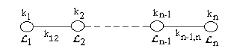
Figure 4: This is a geometric representation of a multilayer FQH state. Each a-th node, of the diagram $\left\{\cup_{b=1}^{n}{\mathcal{L}}_{b}\right\}$,  describes a layer ${\mathcal{L}}_{a}$; viewed as a spherical $D2$ brane with filling factor $k_{a}$.  Nodes are associated with the a-th projector $\pi_{a}$  on the $n$ dimensional basis vector $|a>$  and the filling factor $k_{a}$.  Interactions between layers are restricted to the closest ones $\left(\mathcal{L}_{a},\mathcal{L}_{a\pm 1}\right)$ and are encoded in the links $u_{ab}=|a><b|$ with integral coefficients $k_{ab}$.  Such diagram, which is of the ordinary $A_{n-1}$  type classification, has a formal similarity with the geometric engineering of the Coulomb branch of N=2 supersymmetric theories [34, 35].

Having fixed our terminology and convention notations, we now turn to study the effective field models for multilayer states occupying the first Landau level of the system; but also those general states occupying several Landau levels.

3 FQH Effective Field Model

As we have several situations depending on the number of layers as well as the number of Landau levels on the layers represented by the fiber bundles $\left\{\cup_{a=1}^{n}\left\{\cup_{i_{a}=1}^{m_{a}}{LL}_{i_{a}};\mathcal{L}_{a}\right\}\right\}$, one may distinguish different kinds of interactions coming from:

(i) the internal structure of the base manifold B$=\cup_{a=1}^{n}\mathcal{L}_{a}$, which in the case of coincident layers lead a priori non abelian symmetries generated by $\left\{|a><b|\right\}$ as in we usually have in Brane systems.

(ii) couplings of the fibers F=$\cup_{i_{a}=1}^{m_{a}}{LL}_{i_{a}}$ living on the base manifold. In the case where all layers are in the Laughlin ground states for instance; that is a fiber bundle of the form $\cup_{a=1}^{n}\left\{{LL}_{1};\mathcal{L}_{a}\right\}$; fbers interactions are encoded in the intersection matix $\alpha_{a}.\alpha_{b}=\mathrm{G}_{ab}$.

(iii) both from the base B and the fiber F.

We will then adopt the following strategy in studying the effective field model for the multilayer systems. First we suppose that all layers of the system are of Laughlin type and describe the commutative field approach. Then, we study its non commutative extension using Susskind method. Once this done, we consider the case a single layer; but with several Landau levels. Here also we study first the commutative field model; and then we analyze its non commutative extension. Finally, we consider the case of several layers and several Landau levels.

3.1 Multilayer Commutative Field Model

To get the generalized effective field model describing multilayer FQH states, one should specify the condition on $\left|d_{a}-d_{b}\right|$ spacings. The point is that the $A_{\mu}$ gauge fields on the multilayers have, in addition to the $n\times n$ matrix structure, a dependence on the $y_{a}^{\mu}=\left(y^{1},y^{2},y^{3}=d_{a}\right)$ coordinates of the $n$ layers, viewed as parallel $D2$ branes. According to the values of $\left|d_{a}-d_{b}\right|$, one distinguishes several cases lying between the completely abelian model with a $U\left(1\right)^{n}$ gauge symmetry and the largest non abelian $U\left(n\right)$ invariance.

3.1.1 Abelian model

If for example, one supposes that $\left|d_{a}-d_{b}\right|>>>1,\quad\forall a,b=1,...,n$; that is all layers are very distant from each others, then layers interactions may be ignored and one is left with a $U\left(1\right)^{n}$ model.

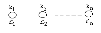
Figure 5: This figure represents a system of $\mathit{n}$ parallel layers very distant from each others. They describe $n$ uncoupled FQH states with filling factor $\nu_{a}=1/k_{a}$. The gauge field are given by the diagonal terms and the gauge symmetry is $U(1)^{n}$. The total filling factor of the system is just the sum.

In this system, each one of the layers ( $D2$ brane ), partially filled with $\nu_{a}$ of the form $\frac{1}{k_{a}}$, $k_{a}$ odd integer, describes an electronic system with a conserved number $\mathcal{N}_{a}$ of particles,

$$\frac{d\mathcal{N}_{a}}{dt}=0,$$ (3.1)

In effective field theory, the number $\mathcal{N}_{a}$ of electrons moving on the layer may be also expressed as an integral over the density electron number par surface unit;

$$\mathcal{N}_{a}=\int_{\mathcal{L}_{a}}d^{2}y\text{ }\mathcal{J}_{a}^{0}\left(y,d_{a}\right),$$ (3.2)

where $\mathcal{J}_{a}^{0}\left(y,d_{a}\right)=\partial^{2}\mathcal{N}_{a}/\partial^{2}y$. The condition of conservation (3.1) is ensured by the introduction of a $\left(1+2\right)$ conserved current $\mathcal{J}_{a}^{\mu}$; i. e $\partial_{\mu}\mathcal{J}_{a}^{\mu}=\partial_{0}\mathcal{J}_{a}^{0}+\partial_{i}\mathcal{J}_{a}^{i}=0$ leading to

$$\frac{d\mathcal{N}_{a}}{dt} = -\int_{\mathcal{L}_{a}}d^{2}y\partial_{i}\mathcal{J}_{a}^{i}$$ (3.3)

$$= -\frac{1}{2\pi}\oint_{\partial\mathcal{L}_{a}}dl_{i}A_{i}^{a},$$ (3.4)

which vanishes provided the boundary $\partial\mathcal{L}_{a}$ of the layer is zero, or the $A_{a}^{i}$ field vanishes on $\partial\mathcal{L}_{a}$ or again due to the existence of some periodicity features. The equality of eq(3.4), using the hypothesis $\mathcal{J}_{a}^{i}=\frac{1}{2\pi}\varepsilon^{0ij}\partial_{i}A_{j}^{a}$, reflects just the Chern Simons field realization of the $\mathcal{J}_{a}^{\mu}$ conserved current, which reads as,

$$\mathcal{J}_{a}^{\mu}\left(y,d_{a}\right)=\frac{1}{2\pi}\varepsilon^{\mu\nu\sigma}\partial_{\nu}A_{\sigma}^{a};\quad a=1,...,n,$$ (3.5)

Since the layers $\mathcal{L}_{a}$ are partially filled with filling factor$1/\mathrm{k}_{a}$, we should have the remarkable relations,

$$\mathrm{k}_{a}\mathcal{N}_{a}=\mathcal{N}_{\phi};\quad a=1,...,n,$$ (3.6)

which, in the framework of the Chern Simons model, this is just the equation of motion of the time component of the gauge fields; that is

$$\mathrm{k}_{a}\frac{1}{2\pi}\varepsilon^{0\nu\sigma}\partial_{\nu}A_{\sigma}^{a}=\frac{1}{2\pi}\varepsilon^{0\nu\sigma}\partial_{\nu}\mathcal{A}_{\sigma},$$ (3.7)

without summation on the repeated index $a$. The original formal action, invariant under the gauge changes $\delta A_{\mu}^{a}=\partial_{\mu}\lambda^{a}$, and leading to the above eq of motion is,

$$S\left[A_{\mu}^{a},\mathcal{A}_{\mu}\right] = \frac{\mathrm{1}}{4\pi}\int d^{3}y\varepsilon^{\mu\nu\sigma}\sum_{a=1}^{n}\mathrm{k}_{a}A_{\mu}^{a}\partial_{\nu}A_{\sigma}^{a}$$ (3.8)

$$-\frac{\mathrm{1}}{2\pi}\int d^{3}y\varepsilon^{\mu\nu\sigma}\left(\sum_{a=1}^{n}A_{\mu}^{a}\right)\partial_{\nu}\mathcal{A}_{\sigma}.$$

Note that the right way one should think about this action is in terms of the field diagonal matrices,

$$A_{\mu}=\sum_{a=1}^{n}A_{\mu}^{a}\pi_{a};\quad\pi_{a}=|a><a|,$$ (3.9)

where $\pi_{a}$’s are the projectors on the layers. In terms of these matrices, the previous action may be rewritten in a more interesting form as,

$$S\left[A_{\mu}^{a},\mathcal{A}_{\mu}\right]=\frac{\mathrm{1}}{4\pi}\int d^{3}y\varepsilon^{\mu\nu\sigma}\left[Tr\left(\mathrm{\kappa}A_{\mu}\partial_{\nu}A_{\sigma}-2A_{\mu}\partial_{\nu}\mathcal{A}_{\sigma}\right)\right],$$ (3.10)

Here $\mathrm{\kappa}$ is the coupling matrix, itself a $n\times n$ diagonal matrix,

$$\mathrm{\kappa=}\sum_{a=1}^{n}\mathrm{k}_{a}\pi_{a}.$$ (3.11)

By help of the $A_{\sigma}$ and $\mathrm{\kappa}$ matrices, the new eq of motion following from the action(3.10) is,

$$\mathrm{\kappa}\frac{1}{2\pi}\varepsilon^{0\nu\sigma}\partial_{\nu}A_{\sigma}=\frac{1}{2\pi}\varepsilon^{0\nu\sigma}\partial_{\nu}\mathcal{A}_{\sigma},$$ (3.12)

which, upon integration over $d^{2}y$, gives the $n\times n$ matrix eq

$$\mathrm{\kappa}\mathcal{N}\mathrm{=}\mathcal{N}_{\phi}I;\quad\quad\mathcal{N}\mathrm{=}\mathcal{N}_{a}\pi_{a}$$ (3.13)

Taking the trace over this relation, one gets the total filling factor

$$\mathrm{\nu} = Tr\left(\mathrm{\kappa}^{-1}\right)$$

$$= \sum_{a=1}^{n}\frac{1}{\mathrm{k}_{a}}.$$

Remember the first term of this relation; we shall see that it is also valid in presence of interactions and whether the gauge symmetry is abelian or not. Note that the appearance of the $\mathrm{\kappa}$ coupling matrix seems a little bit strange. In fact this is a very special point inherent to the $U\left(1\right)^{n}$ abelian symmetry generated by the projectors $\pi_{a}$. In the non abelian case, the coupling should, under some conditions to be specified in subsubsection 3.1.2 when studying the second kind of solutions, be an integer. Before that let us first derive the appropriate constraint eqs linking gauge symmetry and filling factors and then return to complete the comment regarding eq(3.1.1).

3.1.2 Non abelian Case

Non abelian FQH systems appear in presence of interactions between the $\mathcal{L}_{a}$ layers of the system $\left\{\cup_{a=1}^{n}\mathcal{L}_{a}\right\}$, as in the special case where all layers are quasi coincident; i.e all parameters $d_{a}\sim d_{1}$; i.e

$$\left|d_{a}-d_{b}\right|<<<1,\quad\forall a,b=1,...,n,$$ (3.15)

or more generally as in cases where subsets $\left\{\cup_{a_{s}=1}^{r}\mathcal{L}_{a_{s}};r<n\right\}$ of the layers are closed enough to each others while the remaining others $\left\{\cup_{a_{s}=r+1}^{n}\mathcal{L}_{a_{s}};\right\}$ are far away;

$$\left|d_{a_{s}}-d_{b_{s}}\right|<<<1,\quad a_{s},b_{s}\in J_{r}\subset\left[1,n\right].$$ (3.16)

In this case, the $N_{a}$ numbers are no longer constants of motion since particles can travel from a given layer $\mathcal{L}_{a}$ to an other closed $\mathcal{L}_{b}$ one. To illustrate this feature more explicitly, let $\mathcal{N}$ denote the total number of electrons moving in the multilayer system,

$$\mathcal{N}=\sum_{a=1}^{n}N_{a}.$$ (3.17)

Because of interaction between layers, this number can usually written as the trace over a $n\times n$ matrix $\mathbf{N=}\left(\mathbf{N}_{ab}\right)$, in complete harmony with the previous case where interactions were ignored,

$$\mathcal{N}=Tr\mathbf{N=}\sum_{a=1}^{n}N_{a}$$ (3.18)

In fact the effective number $\widetilde{N}_{a}$ of electrons moving on a given layer $\mathcal{L}_{a}$, at a given time, is the sum of three terms; namely the initial number $N_{a}$ plus the number $N_{ab}$ of electrons leaving the $\left(n-1\right)$ layers $\mathcal{L}_{b}$ of the system and landing on $\mathcal{L}_{a}$ minus the number $N_{ba}$ of electrons leaving $\mathcal{L}_{a}$ for the other $\mathcal{L}_{b}$ layers,

$$\widetilde{N}_{a}=N_{a}+\sum_{b=1,b\neq a}^{n}N_{ab}-\sum_{b=1,b\neq a}^{n}N_{ba};\quad a=1,...,n,$$ (3.19)

This relation may be also rewritten, by adding and subtracting the numbers $N_{a}\equiv N_{aa}$, as follows

$$\widetilde{N}_{a}=N_{a}+\sum_{b=1}^{n}\left(N_{ab}-N_{ba}\right);\quad a=1,...,n,$$ (3.20)

Summing over all $\widetilde{N}_{a}$’s, one discovers the following conserved quantity,

$$\mathcal{N}=\sum_{a=1}^{n}\widetilde{N}_{a}=\sum_{a=1}^{n}N_{a}$$ (3.21)

To get the effective field model describing the multilayer FQH states with interactions; we shall follow the method we have developed above by expressing the constant of motion $\mathcal{N}$ as an integral over a density $\mathcal{\rho}$ of a conserved current $\mathcal{J}^{\mu}$; that is

$$\mathcal{N} = \int_{\cup\mathcal{L}_{a}}d^{2}y\text{ }\mathcal{\rho};$$ (3.22)

$$0 = \partial_{0}\mathcal{\rho}+\partial_{i}\mathcal{J}^{i}.$$ (3.23)

Since the FQH system $\left\{\cup_{a=1}^{n}\mathcal{L}_{a}\right\}$ has interactions one expects, from the similarity between $\left\{\cup_{a=1}^{n}\mathcal{L}_{a}\right\}$ and the assembly of $n$ parallel $D2$ branes, that the underlying theory is, roughly speaking, a non abelian Chern Simons $U\left(n\right)$ gauge model. This is indeed what one gets if one does not worry about the details of FQH physics on each layer and insists on $U\left(n\right)$ gauge symmetry. Indeed having $U\left(n\right)$ gauge invariance requires coincident $D2$ branes but moreover the same filling factor. To get the point let us set the problem in its general form and work out explicitly the link between gauge invariance and layers filling factors.

• Constraint Eqs

Since the total number $\mathcal{N}$ of electrons is a constant of motion following from the existence of a Noether conserved current $\mathcal{J}^{\mu}$ and since $\mathcal{N}$ has the form of a trace (3.18), let us write $\mathcal{J}^{\mu}$ as

$$\mathcal{J}^{\mu}=\mathrm{Tr}\mathbf{J}^{\mu},$$ (3.24)

where $\mathbf{J}^{\mu}$ is a $n\times n$ hermitian matrix. Moreover, since it is the trace $\mathrm{Tr}\mathbf{J}^{\mu}$ that should be conserved and not necessary the matrix $\mathbf{J}^{\mu}$; one may in general realize this matrix field in terms of the non abelian Chern Simons potential as,

$$\mathbf{J}^{\mu}=\frac{1}{2\pi}\varepsilon^{\mu\nu\sigma}\left(\mathbf{P.}\partial_{\nu}\mathbf{A}_{\sigma}+i\mathbf{Q.}\left[\mathbf{A}_{\nu},\mathbf{A}_{\sigma}\right]\right),$$ (3.25)

where the couplings $\mathbf{P}$ and $\mathbf{Q}$ are a priori arbitrary invertible and hermitian $n\times n$ matrices with integer entries; that is $\mathbf{P,Q\in}Gl\left(n,Z\right)$. Although the idea of taking $\mathbf{P}$ and $\mathbf{Q}$ couplings as matrices seems going against what is established in non abelian Chern Simons gauge theory; it is however a physical argument extending eq(3.11) which allows us to get the constraint eqs between gauge invariance and the filling factors of the layers. So $\mathbf{P}$ and $\mathbf{Q}$ as matrices is dictated by the fact that we want to insert in the effective gauge field model, we looking to build, the fact that layers may have different filling factors. Requiring non abelian gauge invariance, which acts as,

$$\mathbf{A}^{\prime} = \mathbf{U}^{-1}\left(\mathbf{A}-\partial\right)\mathbf{U};$$

$$\mathbf{J}^{\mu\prime} = \mathbf{U}^{-1}\mathbf{J}^{\mu}\mathbf{U,}$$ (3.26)

where $\mathbf{U}$ is a $n\times n$ matrix defining the gauge transformations as well as the condition of current conservation $\partial_{\mu}\mathcal{J}^{\mu}=0$, we get the following constraint eqs,

$$\mathbf{U}^{-1}\mathbf{PU} = \mathbf{P,}$$ (3.27)

$$\mathbf{U^{-1}QU} = \mathbf{Q,}$$ (3.28)

and

$$\frac{1}{2\pi}\varepsilon^{\mu\nu\sigma}\partial_{\mu}\mathrm{Tr}\left(\mathbf{P.}\partial_{\nu}\mathbf{A}_{\sigma}+i\mathbf{Q.}\left[\mathbf{A}_{\nu},\mathbf{A}_{\sigma}\right]\right)=0,$$ (3.29)

The two first constraint eqs (3.27,3.28) reflect the fact that $\mathbf{P}$ and $\mathbf{Q}$ should be gauge invariant in order to be interpreted as physical coupling constants; while the third one (3.29) implies that the total number of particles is a constant of motion. Since $\mathbf{U}$ is an arbitrary gauge transformation matrix, these constraint eqs impose a severe restriction on the kind of $\mathbf{P}$ and $\mathbf{Q}$ matrices one can have. Let us explore the possible solutions on illustrating examples.

• Solutions

(1) Solution I: Non Abelian $U\left(n\right)$ Chern Simons model

If we insist on having $U\left(n\right)$ gauge invariance, that is $\mathbf{U}$ an arbitrary $n\times n$ unitary matrix, then there is a unique solution that commute with all $U\left(n\right)$ matrix elements. This solution is proportional to the identity as required by the Schur lemma; that is a number $\mathrm{k}$ times the identity operator

$$\mathbf{P=}\mathrm{k}^{\prime}\text{ }\mathbf{\mathrm{I;\quad}Q=}\mathrm{k}^{\prime\prime}\text{{\ }}\mathbf{\mathrm{I}}\text{,}$$ (3.30)

Unitarity require moreover that k=$\mathrm{k}^{\prime}/\mathrm{k}^{\prime\prime}$ should be positive integer. In this case the solution for $\mathbf{J}^{\mu}$ in terms of the $U\left(n\right)$ gauge potentials $\mathbf{A}_{\mu}$ reads, after setting $\mathrm{k}^{\prime\prime}=1$ or absorbing it in the gauge field ( $\mathbf{A\rightarrow}\mathrm{k}^{\prime}\mathbf{A}$ ), as

$$\mathbf{J}^{\mu} = \frac{\mathrm{k}}{2\pi}\varepsilon^{\mu\nu\sigma}\left(\partial_{\nu}\mathbf{A}_{\sigma}+i\left[\mathbf{A}_{\nu},\mathbf{A}_{\sigma}\right]\right),$$ (3.31)

$$\mathbf{J}^{0} = \frac{\mathrm{k}}{2\pi}\varepsilon^{0\nu\sigma}\left(\partial_{\nu}\mathbf{A}_{\sigma}+i\left[\mathbf{A}_{\nu},\mathbf{A}_{\sigma}\right]\right)$$ (3.32)

Note that though non abelian, the $\mathbf{J}^{0}$ time component may also be put in the useful form,

$$\mathbf{J}^{0}=\frac{\mathrm{k}}{2\pi}\mathbf{B}$$ (3.33)

where now the $n\times n$ matrix $\mathbf{B}$ is the curl of the non abelian gauge potential field $\mathbf{A}_{\mu}$. Observe in passing that while $\mathcal{J}^{\mu}=\mathrm{Tr}\mathbf{J}^{\mu}$ is conserved due to the obvious property $\mathrm{Tr}\left[\mathbf{A}_{\nu},\mathbf{A}_{\sigma}\right]=0$, the $\mathbf{J}^{\mu}$ vector field is not conserved in the usual sense since in general $\partial_{\mu}\left(\varepsilon^{\mu\nu\sigma}\left[\mathbf{A}_{\nu},\mathbf{A}_{\sigma}\right]\right)$ is different from zero. This property reflects the fact that the numbers $N_{a}$ of particles on  each layer $\mathcal{L}_{a}$ are not constants of motion in the usual sense. The $\mathbf{J}^{\mu}$ current obeys however a covariantly conserved relation namely,

$$D_{\mu}\mathbf{J}^{\mu}=\partial_{\mu}\mathbf{J}^{\mu}-i\left[\mathbf{A}_{\mu},\mathbf{J}^{\mu}\right]=0.$$ (3.34)

Moreover, from the identity $\mathcal{N}=\nu\mathcal{N}_{\phi}$, or again by equating the current densities, we have,

$$\frac{\mathrm{k}}{2\pi}\mathbf{B}=\frac{\mathrm{1}}{2\pi}\mathcal{B}_{ex}.\mathrm{I}$$ (3.35)

This relation reads in terms of the non abelian $\mathbf{A}$ gauge fields and the $\varepsilon^{0\nu\sigma}$ antisymmetric tensor as,

$$\frac{\mathrm{k}}{2\pi}\varepsilon^{0\nu\sigma}\left(\partial_{\nu}\mathbf{A}_{\sigma}+i\left[\mathbf{A}_{\nu},\mathbf{A}_{\sigma}\right]\right)=\frac{\mathrm{1}}{2\pi}\varepsilon^{0\nu\sigma}\partial_{\nu}\mathcal{A}_{\sigma}.\mathrm{I,}$$ (3.36)

This way of writing shows that one is dealing just with the equation of motion of the time component $\mathbf{A}_{0}$ of the gauge field $\mathbf{A}_{\mu}$. This eq together with the two remaining others recovered under $SO\left(1,2\right)$ covariance, follow from the action the non abelian $U\left(n\right)$ Chern Simons gauge field theory,

$$S\left[A_{\mu},\mathcal{A}_{\mu}\right] = \frac{\mathrm{k}}{4\pi}\int d^{3}y.\varepsilon^{\mu\nu\sigma}\mathrm{Tr}\left(\mathbf{A}_{\mu}\partial_{\nu}\mathbf{A}_{\sigma}+\frac{2i}{3}\mathbf{A}_{\mu}\left[\mathbf{A}_{\nu},\mathbf{A}_{\sigma}\right]\right)$$ (3.37)

$$-\frac{\mathrm{1}}{2\pi}\int d^{3}y.\varepsilon^{\mu\nu\sigma}\mathrm{Tr}\left(\mathbf{A}_{\mu}\partial_{\nu}\mathcal{A}_{\sigma}\right)$$

The filling fraction of the multilayer system is

$$\mathrm{\nu}=\frac{1}{\mathrm{k}}\mathrm{Tr}\left(\mathbf{I}\right)\mathrm{=}\frac{n}{\mathrm{k}}.$$ (3.38)

This result, which was expected from general features of non abelian Chern Simons gauge theory and branes physics, may be exploited to derive the general expression of the filling factors  associated with FQH multilayer states having a gauge symmetry contained in $U\left(n\right)$. The general result relating the filling factor to the $U\left(n\right)$ gauge subgroups is summarized in the following table.

Gauge Group $$U\left(1\right)^{n}$$

Filling factor

(3.39)

From this table we learn, amongst others , that the filling fraction of a FQH  $n$ layers state with gauge symmetry $U\left(n-m\right)\times U\left(m\right)$ reads in general as

$$\mathrm{\nu}=\frac{n-m}{k_{1}}+\frac{m}{k_{2}}.$$ (3.40)

This relation tells us that the multilayer system is made of $\left(n-m\right)$ coincident layers with individual filling factor $1/k_{1}$ and $m$ coincident layers with individual filling factor $1/k_{2}$. A necessary condition to have $U\left(n\right)$ gauge invariance is then $k_{1}=k_{2}$; that is layers with same filling factors. If one insists of having layers with different filling factors; $U\left(n\right)$ gauge symmetry is automatically broken down to $U\left(n\right)$ subgroups. This property can be learnt on the way we solve the constraint eqs. Let us comment a little bit this important point by explicit computation of the second type of solutions.

(2) Solution II : Non abelian $U\left(n\right)$ Chern Simons model broken down to a subgroup $G$

If one is not interested in having an exact $U\left(n\right)$ invariance, the constraint equations (3.27,3.28) may be solved by restricting to $\mathbf{U}$ gauge transformations in subgroups of $U\left(n\right)$.

(a) Case $G=U\left(1\right)^{n}\subset U\left(n\right)$

In case where all layers have different filling factors, the underlying $U\left(n\right)$ gauge group is broken down to $U\left(1\right)^{n}$; see figure 6. In this configuration, the $n\times n$ unitary matrix transformation $\mathbf{U}$ have the following diagonal form,

$$\mathbf{U=}\left(\begin{array}[]{cccc}\exp i\phi_{1}&&&\\ &.&&\\ &&.&\\ &&&\exp i\phi_{n}\end{array}\right),$$

and so eqs(3.27,3.28) are automatically fulfilled. However, the current conservation condition (3.29), although does not affect the $\mathbf{P}$ matrix, still requires that the $\mathbf{Q}$ matrix should satisfy,

$$\frac{1}{2\pi}\varepsilon^{\mu\nu\sigma}\partial_{\mu}\mathrm{Tr}\left(\mathbf{Q.}\left[\mathbf{A}_{\nu},\mathbf{A}_{\sigma}\right]\right)=0,$$ (3.41)

which is filled if and only if the matrix $\mathbf{Q}$ is proportional to the identity. In this case, the current density $\mathbf{J}^{0}$ may be solved, by setting $\mathbf{Q=I}$ and $\mathbf{P=}$ $\mathrm{\kappa}$, as

$$\mathbf{J}^{0}=\frac{1}{2\pi}\varepsilon^{0\nu\sigma}\left[\mathrm{\kappa}\left(\partial_{\nu}\mathbf{A}_{\sigma}+i\mathrm{\kappa}^{-1}\left[\mathbf{A}_{\nu},\mathbf{A}_{\sigma}\right]\right)\right],$$ (3.42)

and the the relation $\mathcal{N}=\mathcal{\nu N}_{\phi}$ as well as its $SO\left(1,2\right)$ covariance give

$$\frac{1}{2\pi}\varepsilon^{\mu\nu\sigma}\left[\mathrm{\kappa}\left(\partial_{\nu}\mathbf{A}_{\sigma}+i\mathrm{\kappa}^{-1}\left[\mathbf{A}_{\nu}\mathbf{,A}_{\sigma}\right]\right)\right]=\frac{1}{2\pi}\varepsilon^{\mu\nu\sigma}\partial_{\nu}\mathcal{A}_{\sigma}.\mathrm{I,}$$ (3.43)

which is nothing but the equation of motion one gets from the following action

$$S\left[A_{\mu},\mathcal{A}_{\mu}\right]=\frac{\mathrm{1}}{4\pi}\int d^{3}y.\varepsilon^{\mu\nu\sigma}\mathrm{Tr}\left(\mathrm{\kappa}\mathbf{A}_{\mu}D_{\nu}\mathbf{A}_{\sigma}\mathbf{-}2\mathbf{A}_{\mu}\mathbf{D}_{\nu}\mathcal{A}_{\sigma}\right)$$ (3.44)

where we have set $D_{\nu}=\mathrm{I.}\partial_{\nu}+\frac{2i}{3}\mathrm{\kappa}^{-1}\left[\mathbf{A}_{\nu},\right]$. Under a $U\left(1\right)\subset U\left(n\right)$ gauge transformation

$$\mathbf{A}_{\sigma}^{\prime}=\mathbf{A}_{\sigma}+\partial_{\sigma}\lambda.\mathrm{I;\quad\quad}\left[\mathbf{A}_{\nu},\partial_{\sigma}\lambda.\mathrm{I}\right]=0$$ (3.45)

the terms appearing in the above action, namely $D_{v}\mathbf{A}_{\sigma}$ and $\mathbf{A}_{\mu}D_{\nu}\mathbf{A}_{\sigma}$, transform as

$$D_{v}^{\prime}\mathbf{A}_{\sigma}^{\prime} = D_{v}\mathbf{A}_{\sigma}+\mathrm{I.}\partial_{\nu}\partial_{\sigma}\lambda,$$

$$\mathbf{A}_{\mu}^{\prime}D_{\nu}^{\prime}\mathbf{A}_{\sigma}^{\prime} = \mathbf{A}_{\mu}D_{\nu}\mathbf{A}_{\sigma}+\mathrm{I.}\partial_{\mu}\partial_{\nu}\partial_{\sigma}\lambda,$$ (3.46)

and so invariance of the functional eq(3.44) is ensured by the completely antisymmetric factor $\varepsilon^{\mu\nu\sigma}$. The filling fraction formula

$$\mathrm{\nu}=\mathrm{Tr}\left(\mathrm{\kappa}^{-1}\right)$$ (3.47)

for the $U\left(1\right)^{n}$ model with interaction is similar to the one we have got earlier in the case of the multilayer system without interactions. But one should note that while $\mathrm{\kappa}$ is diagonal in the last case; it is however not for the first one allowing extra contributions; see figure 6.

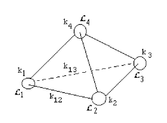
Figure 6:  This figure represents a system of $n=4$ layers with mutual interactions. The general graph on gets is a simplex of four vertices and six edges. The coupling matrix has in general ten free integers $k_{ab}=k_{ba}$  and the filling fraction is given by eq(3.47). Subsystems of this configuration are obtained by making choices on the integers $k_{ab}$  such as for instance identifying the quantum numbers carried by two vertices and their link.

(b)  General Case $G\subset U\left(n\right)$

To see how the solution of the constraint eqs (3.27,3.28,3.29) for generic subgroups of $U\left(n\right)$, let us consider the example where $U\left(n\right)$ is broken down to $U\left(2\right)\times U\left(1\right)^{n-2}$. In this case, the $n\times n$ unitary matrix transformation $\mathbf{U}$ have the following diagonal form

$$\mathbf{U=}\left(\begin{array}[]{cccccc}u_{11}&u_{12}&0&&&0\\ u_{21}&u_{22}&0&&&0\\ 0&0&\exp i\phi_{1}&&&\\ &&&.&&\\ &&&&.&\\ 0&0&&&&\exp i\phi_{n-2}\end{array}\right),$$

where $u_{ij}$, $\left|u_{11}u_{22}-u_{12}u_{21}\right|=1$, are elements of $U\left(2\right)$ and $\phi_{a}$ phase of $U\left(1\right)^{n-2}$. While the matrix $\mathbf{Q}$ is usually proportional to the identity, the matrix $\mathbf{P=}$ $\mathrm{\kappa}$ should the form

$$\mathrm{\kappa=}\left(\begin{array}[]{ccc}k&0&k_{1a}\\ 0&k&k_{2a}\\ k_{1a}&k_{2a}&\mathrm{\kappa}^{\prime}\end{array}\right)$$

where $\mathrm{\kappa}^{\prime}$ is a $\left(n-2\right)\times\left(n-2\right)$ hermitian matrix. By repeating this analysis, one gets all possible configurations. For the special case where $k_{1a}=k_{2a}=0$, one has a reducible diagram.

• Examples

To illustrate the prediction of broken $U\left(n\right)$ gauge models, let us consider two examples; the first one concerns two layers FQH states and the second one involves three layers.

(a) Two layers States

In the example of two coupled layers $\mathcal{L}_{1}$ and $\mathcal{L}_{2}$ with the hermitian coupling matrix $\mathrm{\kappa}$, reads as

$$\mathrm{\kappa=}\left(\begin{array}[]{cc}k_{1}&l\\ l&k_{2}\end{array}\right)$$ (3.48)

where $k_{1}$, $k_{2}$ are odd integers and, a priori, $l$ is any positive integer; see figure 7

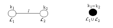
Figure 7: This is the quiver diagram of two layers FQH states. For different values of $k_{1}$ and $k_{2}$ and the field model has a $U(1)^{2}$ abelian symmetry  the total filling factor of the system is given by eq(3.48). Non abelian $U(2)$  model is obtained for $k_{1}=k_{2}=k$ and $k_{12}=0$.

In this case filling factor $\mathrm{\nu}$, that follows from eq(3.47), is given by the following three integer series,

$$\mathrm{\nu}=\frac{k_{1}+k_{2}}{k_{1}k_{2}-l^{2}}$$ (3.49)

This is a general relation containing as special cases known results on FQH states with two levels. Setting $l=0$, one gets the familiar relation $\mathrm{\nu}=1/k_{1}+1/k_{2}$ of uncoupled $U\left(1\right)^{2}$ FQH states which gets an enhanced $U\left(2\right)$ symmetry for $k_{1}=k_{2}=k$. One may also recover the Jain series $2/\left(4p\pm 1\right)$ at level two by taking

$$k_{1}=k_{2}=k;\quad l^{2}=nk;\quad k-n=4p\pm 1$$ (3.50)

As an explicit example, one sees that the solutions for the state $\mathrm{\nu}=2/5$ reproduce all known results. Expressing $l$ in terms of $k_{1}$ and $k_{2}$, one gets a constraint relation on the values of $l$ integers one should have for $\mathrm{\nu}=2/5$,

$$l=\frac{1}{2}\sqrt{\left(2k_{1}-5\right)\left(2k_{2}-5\right)-25};\quad l\in Z^{+}.$$ (3.51)

The solutions are as follows: (i) $k_{1}=k_{2}=k$ and $l=\sqrt{k\left(k-5\right)}$ which is fulfilled for $l=0$ and $k=5$ ; but also $l=6$ and $k=9$. The first solution corresponds to the multilayer system$\left(550\right)$ in terms of the conventional classification made in [29]; while the second corresponds to $\left(332\right)$. (ii) There is also an other solution for $k_{1}=3$, $k_{2}=15$ and $l=0$ in a complete agreement with Haldane result, to be discussed later on. The same is also valid for $\mathrm{\nu}=2/3$ where the integrality condition on $l$ reads as

$$l=\frac{1}{2}\sqrt{\left(2k_{1}-3\right)\left(2k_{2}-3\right)-9};\quad l\in Z^{+}.$$ (3.52)

A general result can be written down for all terms of the Jain sequence; see eq(1.6).

(b) Three layers States

For the case of three layers, the matrix $\mathrm{\kappa}$ has in general three odd $k_{a}$ integers associated with self interactions and three other integers $l$, $m$, $t$ associated with the three kinds of couplings; see figure 8.

$$\mathrm{\kappa=}\left(\begin{array}[]{ccc}k_{1}&l&m\\ l&k_{2}&t\\ m&t&k_{3}\end{array}\right).$$ (3.53)

This is a real symmetric matrix whose diagonal elements $k_{a}$ are positive odd integers giving the filling factors of the layers in lowest Landau level configuration. The off diagonal entries encode layers interactions.

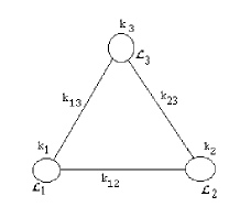
Figure 8: Here we give the diagram for FQH states involving three layers in the first Landau level. The filling fraction is given by eq(3.53). For $k_{a}\neq k_{b}\neq k_{c}$ and $k_{ab}=k_{ac}=k_{bc}=0$  we have an abelian $U(1)^{3}$ symmetry without layers interactions. In the other cases there are interactions and in general the symmetry may be non abelian. In the case $k_{a}=k_{b}=k_{c}$ and $k_{ab}=k_{ac}=k_{bc}=0$, we have the largest symmetric $U(3)$ non abelian gauge model.

This matrix depends on $\left(3+3\right)=6$ integers allowing to classify the three kinds of effective field models one has in this case; see figure 9.

$\left(\alpha\right)$ Model with $U\left(1\right)^{3}$ symmetry.

Here, the $k_{a}$ integers are different and $l$, $m$ and $t$ are generally non zero. The filling factor one gets depends then on $\left(3+3\right)$ integers and reads in general as,

$$\mathrm{\nu}=\frac{\left(k_{2}k_{3}+k_{1}k_{3}+k_{1}k_{2}\right)-\left(l^{2}+m^{2}+t^{2}\right)}{k_{1}k_{2}k_{3}+2lmt-\left(k_{1}t^{2}+l^{2}k_{3}+m^{2}k_{2}\right)}$$ (3.54)

Special cases may be also considered here; like for instance retaining only couplings dealing with closer neighboring layers by setting $m=0$ or again by setting $l=t$ and $m=0$.

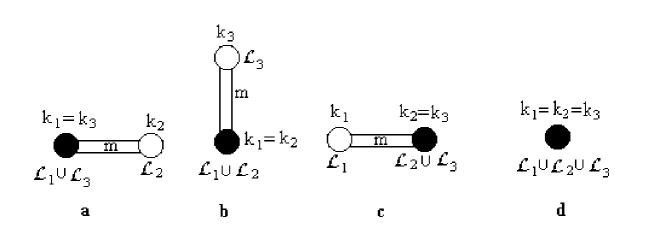
Figure 9: Figures 9a, 9b and 9c are obtained from figure 8 by coinciding two nodes giving then a enhanced $U\left(2\right)$ symmetry. For the case $k_{a}=k_{b}\neq k_{c}$, $U\left(2\right)$ symmetry requires $k_{ab}=0$ but $k_{ac}=k_{bc}$. In figure 9d, the three nodes are coincident and the symmetry is $U\left(3\right)$.

$\left(\beta\right)$ Models with $U\left(1\right)\times U\left(2\right)$ symmetry.

Here, two of the three $k_{a}$ integers are equal and one of the $l$, $m$ and $t$ integers is zero and the remaining two others are equal. For instance, we can have $k_{1}=k_{2}=k$ and $l=0$ together with $m=t$. In this configuration, which is associated with the diagram of figure 9b, the filling factor one gets depends then on $3$ integers $k$, $k_{3}$ and $m$ and reads in general as,

$$\mathrm{\nu}=\frac{k^{2}-2m^{2}+2kk_{3}}{k^{2}k_{3}-2km^{2}}=\mathrm{\nu}_{U\left(2\right)}+\mathrm{\nu}_{U\left(1\right)}$$ (3.55)

This relation may also be decomposed as $\mathrm{\nu}=\mathrm{\nu}_{U\left(2\right)}+\mathrm{\nu}_{U\left(1\right)}$ with,

$$\mathrm{\nu}_{U\left(2\right)} = \frac{2k_{3}}{kk_{3}-2m^{2}}$$

$$\mathrm{\nu}_{U\left(1\right)} = \frac{k^{2}-2m^{2}}{k^{2}k_{3}-2km^{2}}$$ (3.56)

In absence of layer interactions; that is for m=0; the above eqs reduce to the standard situation where one of the layers is far away and the other two are coincident. The last configuration one can also have corresponds to the special case where $k_{1}=k_{2}=k_{3}=k$ and $l=m=t=0$; see figure 9d. The symmetry of this FQH state is the full $U\left(3\right)$ gauge invariance.

Having given the main idea on the commutative effective field of multilayer FQH states with rational values, we pass now to make some comments regarding the wave function approach, a matter of having a global view on the connection between gauge symmetry, the various generalizations of the Laughlin wave functions and their filling factors.

3.2 Wave functions

Here we give the generalizations of the Laughlin wave function for uncoupled and coupled layers using the correspondence layer $\mathcal{L}\longleftrightarrow D2$ brane and the classification in terms of subgroups of $U\left(n\right)$ gauge symmetry.

3.2.1 Uncoupled Layers: $U\left(1\right)^{n}$ model I

For the case where the $n$ layers are enough distant from each others, $\left|d_{a+1}-d_{a}\right|\equiv\epsilon_{a}>>0$, that is in absence of layer interactions, the total wave function $\Psi_{f}$ describing the ground state of the multilayer system is given by the antisymmetric product of individual Laughlin trial waves $\Psi_{La}=\Psi_{L}\left(z_{\alpha_{a}}\right)$

$$\Psi_{f}=\prod_{a=1}^{n}\Psi_{La},$$ (3.57)

where the $\Psi_{La}$ factors are given by,

$$\Psi_{La}=\prod\limits_{\alpha_{a}<\beta_{a}=1}^{N_{a}}\left(z_{\alpha_{a}}-z_{\beta_{a}}\right)^{k_{a}}\exp\left(-\frac{\mathcal{B}_{ex}}{4}\sum_{\gamma_{a}=1}^{N_{a}}\left|z_{\gamma_{a}}\right|^{2}\right),$$ (3.58)

and where $z_{\alpha_{a}}$, $\alpha_{a}=1,...,N_{a}$ are the complex coordinates of electrons on the $a-th$  Laughlin layer $\mathcal{L}_{a}$. Note that antisymmetry of the wave function $\Psi_{f}$ under the change of any pair of electrons requires that all $k_{a}$’s to be odd integer. In this case the filling factor is $\mathrm{\nu}=1/k_{1}+...+1/k_{n}$. The quiver diagram describing this abelian $U\left(1\right)^{n}$ model is given by figure 5.

3.2.2 Coupled Layers:

According to the $\left|d_{b}-d_{a}\right|$ distances between layers $\mathcal{L}_{a}$ and $\mathcal{L}_{b}$,  one can write down different kinds of generalized Laughlin wave function for multilayer system. Here we give the two special ones associated with the field models eqs(3.43) and (3.37). The same reasoning applies to the other configurations. From the analysis of subsection 3.1, we distinguish, amongst others, the following particular models

(1) $U\left(1\right)^{n}$ model II: Layers with different filling factors.

For small distances between the layers; that is for $\mathrm{\epsilon=}\left|d_{b}-d_{a}\right|<<1$, layer couplings are no longer negligible and the generalized Laughlin wave function $\Psi_{coupled}$ describing the ground state of the multilayer system takes a more complicated form. Since the filling factors are not equal, $k_{1}\neq k_{2}\neq...\neq k_{n}$, the $U\left(n\right)$ gauge symmetry, which exist in case where all $k$’s are equal, is now broken down to $U\left(1\right)^{n}$; see figures 6 for illustration.

This model involves, besides the diagonal terms, monomials type $\left(z_{\alpha_{a}}-z_{\beta_{b}}\right)^{\mathrm{k}_{ab}}$ with $a\neq b$ and $\mathrm{k}_{ab}$ some integers. The general form of $\Psi_{coupled}$ extending the Laughlin wave function read then as,

$$\Psi_{coupled}=\prod\limits_{a\leq b=1}^{n}\prod\limits_{\alpha_{a}<\beta_{a}=1}^{N_{a}}\left(z_{\alpha_{a}}-z_{\beta_{b}}\right)^{\mathrm{k}_{ab}}\exp\left(-\frac{B}{4}\sum_{a=1}^{n}\sum_{\gamma_{a}=1}^{N_{a}}\left|z_{\gamma_{a}}\right|^{2}\right)$$ (3.59)

As the layers are closed to each others, electrons may travel from a layer $\mathcal{L}_{a}$ to an other $\mathcal{L}_{b}$ and so antisymmetry, of the wave function under the change of any pair $\left(z_{\alpha_{a}},z_{\beta_{b}}\right)$ of electron coordinates, is no longer a constraint since layers are different. Therefore, the matrix entries $\mathrm{k}_{ab}$ are not required to be odd integers and the total filling factor is given by eq( 3.47). In $n\times n$ matrix notation, the coordinates variables $z_{\alpha_{a}}$ on the $a-th$ layer $\mathcal{L}_{a}$ may be thought of as the $\left(a,a\right)$ diagonal element of $n\times n$ matrix $\mathbf{Z}_{\alpha},$

$$z_{\alpha_{a}}=<a|\mathbf{Z}_{\alpha}\mathbf{|}a\mathbf{>}$$

while the coordinates $z_{\alpha_{ab}}$ of particles traveling from $\mathcal{L}_{a}$ to $\mathcal{L}_{b}$ are just,

$$z_{\alpha_{ab}}=<b|\mathbf{Z}_{\alpha}\mathbf{|}a\mathbf{>}$$

One can use this property to study the cases where the generalized Laughlin wave functions have non abelian symmetries containing the underlying $U\left(n\right)$ gauge symmetry of the coincident $D2$ branes. In what follows, we shall give details for the case of FQH states with full $U\left(n\right)$ symmetry.

(2) Non Abelian $U\left(n\right)$ model

This happens in the case where all layers $\mathcal{L}_{a}$, viewed as $D2$ branes, have the same filling factor $1/k$, $k$ odd integer, the total number $\mathcal{N}$ of electrons moving on $\left\{\cup_{a}\mathcal{L}_{a}\right\}$ may, at a given time, be partitioned into $N_{a}$ particles moving on $\mathcal{L}_{a}$, plus $N_{ab}$ particles leaving $\mathcal{L}_{a}$ for $\mathcal{L}_{b}$ and $N_{ba}$ electrons coming from $\mathcal{L}_{b}$ and landing on $\mathcal{L}_{a}$. These particles form together a $n\times n$ matrix $\mathbf{N}$ with positive integer entries,

$$\mathbf{N}=\left(N_{ab}\right)$$ (3.60)

Note that the total number $\mathcal{N}$ of electrons is given by the trace of this matrix, namely $\mathcal{N}=\mathrm{Tr}\left(\mathbf{N}\right)=N_{1}+...+N_{n}$; see also eqs (3.18-3.21). Moreover as the layers have the same filling factor $1/k$; it follows from $U\left(n\right)$ invariance that, at any time, $N_{1}=...=N_{n}=N$; and so $\mathcal{N}=nN$.

Since on a given layer $\mathcal{L}_{a}$ each electron has a coordinate $z_{\alpha_{a}}$, one can parameterize collectively these particles in a more convenient way by using $n\times n$ matrices. To get the $U\left(n\right)$ invariant Laughlin wave function, we start from eq(3.58) with $k_{1}=...=k_{n}=k$. Then instead of diagonal matrices, we consider a system of $N$ matrices matrices $\left\{\mathbf{Z}_{\alpha}\right\}$ with general entries

$$\mathbf{Z}_{\alpha}=\left(z_{\alpha_{ab}}\right);\qquad a,b=1,...,n$$ (3.61)

where in addition to $z_{\alpha_{aa}}$, the complex coordinates of electrons moving on $\mathcal{L}_{a};$ we have also $z_{\alpha_{ab}}$ and $z_{\alpha_{ba}}$ variables describing respectively the coordinates of the electrons leaving $\mathcal{L}_{a}$ for $\mathcal{L}_{b}$ and the particles coming from $\mathcal{L}_{b}$ to $\mathcal{L}_{a}$. The generalized wave function, taking into account multilayers interactions and invariance under $U\left(n\right)$ symmetry, reads as,

$$\Psi_{U\left(n\right)}=\prod\limits_{\alpha<\beta=1}^{N}\left[\det\left(\mathbf{Z}_{\alpha}-\mathbf{Z}_{\beta}\right)\right]^{\mathrm{k}}\exp\left(-\frac{\mathcal{B}_{ex}}{4}\sum_{\gamma=1}^{N}\mathrm{Tr}\left(\mathbf{Z}_{\gamma}\mathbf{Z}_{\gamma}^{\dagger}\right)\right).$$ (3.62)

Acting by the following $U\left(n\right)$ gauge transformations,

$$\mathbf{Z}_{\alpha}^{\prime}=\mathbf{U}^{-1}\mathbf{Z}_{\alpha}\mathbf{U},$$ (3.63)

invariance of eq(3.62) follows naturally from the global action of the transformations as well as the cyclic property of $\mathrm{det}$ and $\mathrm{trace}$. The filling factor is, in this special case, given by $\mathrm{\nu}=n/k.$

4 NC effective field and matrix models for Multilayer States

We first review briefly the Susskind idea for the case of a single layer with filling factor $1/k$; then we study its extension to the case of the multilayer system in lowest energy configuration. Hierarchies in multilayer states based on non commutative geometry which will be discussed in section 7.

4.1 General on Susskind NC theory

To begin consider an electric charged particle, say an electron, moving in the real plane in presence of an external constant magnetic field $\mathcal{B}_{ex}$. Classically this particle is parameterized by its position $x^{i}(t);\ i=1,2$ and velocity $v^{i}=\partial_{t}{\ x^{i}}$. For a $\mathcal{B}_{ex}$ field strong enough, the dynamics of the particle is mainly governed by the coupling

$$S[x]=\frac{e\mathcal{B}_{ex}}{2}\int dt{\ \varepsilon_{ij}v^{i}x^{j}},$$ (4.1)

which is just the angular momentum of the system, induces at the quantum level a non commutative structure on the real plane; i.e

$$[x^{i},x^{j}]\propto\epsilon^{ij}/\mathcal{B}_{ex}.$$ (4.2)

If we suppose that the total number of electrons $\mathcal{N}_{e}$ is a constant of motion; see footnote 4, thing that we shall use everywhere here, one can write it, in the large $\mathcal{N}_{e}$ limit, as,

$$\mathcal{N}_{e}=\int d^{2}x\mathrm{\rho}=\int d^{2}y\text{ }\mathrm{\rho}_{0},$$ (4.3)

where $\mathrm{\rho}$ and $\mathrm{\rho}_{0}$

$$\mathrm{\rho}_{0}=\left|\frac{\partial^{2}\left(x^{1},x^{2}\right)}{\partial^{2}\left(y^{1},y^{2}\right)}\right|\mathrm{\rho}$$ (4.4)

are the densities of particles in the $\left\{x^{i}\right\}$ and $\left\{y^{i}\right\}$ frames respectively.

In the case of $\mathcal{N}_{e}$ classical particles, without mutual interactions, parameterized by the coordinates $x_{a}^{i}(t)$ and velocities $v_{a}^{i}$, the dynamics is dominated by the $B-x(t)$ couplings extending eq(4.1) as

$$\frac{e\mathcal{B}_{ex}}{2}\int dt\varepsilon_{ij}\ \Sigma_{a=1}^{N}v_{a}^{i}x_{a}^{j},$$ (4.5)

and describing a typical strongly correlated system of electrons showing a quantum Hall effect with filling fraction

$$\mathrm{\nu}=\frac{\mathcal{N}_{e}}{\mathcal{N}_{\phi}};\quad\mathrm{\nu}.\mathcal{N}_{\phi}=\mathcal{N}_{e}.$$ (4.6)

Expressing the number $\mathcal{N}_{\phi}$ of quantum flux, by using the external magnetic field, as

$$\mathcal{N}_{\phi}=\frac{1}{2\pi}\int_{\mathcal{L}}d^{2}y\text{ }\mathcal{B}_{ex}=\frac{1}{2\pi}\oint_{\partial\mathcal{L}}\mathcal{A}^{ex}dl$$ (4.7)

where $\mathcal{B}_{ex}=\varepsilon^{3\mu\nu}\partial_{\mu}\mathcal{A}_{\nu}^{ex}$ and using eq(4.6), one gets relation the density $\mathrm{\rho}_{0}$ of electrons and quantum fluxes, namely $\mathrm{\rho}_{0}=\mathrm{\nu}\frac{\mathcal{B}_{ex}}{2\pi}$.

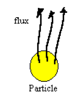
Figure 10: In the Laughlin picture, each electron is coupled with k quantum fluxes as shown on the figure with k=3 . The relation $\nu{\mathcal{N}_{\phi}}={\mathcal{N}_{e}}$ reflects the identity between the densities of electrons and quantum fluxes. As such the conservation of the total number of electrons may be thought of as the charge of the Noether conserved current generating the diffeomorphism symmetry of the y plane or equivalently the gauge symmetry of the Susskind NC effective field model.

Quantum mechanically, there are different field theoretical methods to approach the quantum states of this system, either by using techniques of non relativistic quantum mechanics [36], methods of conformal field theory especially for the study of droplets and edge excitations [31, 32] or again by using the CS effective field model [33] describing the limit $\mathcal{N}\rightarrow\infty$ of electrons where now the Hall system is viewed as a liquid of particles. In this case, the Chern Simons theory in the $(2+1)$ dimensional space modeling the FQH Laughlin state of filling fraction $\nu=\frac{1}{k}$ is obtained by interpreting the $\mathrm{\rho}_{0}$ density as

$$\mathrm{\rho}_{0}=\mathcal{J}^{0}\left(y\right),$$ (4.8)

the time component of a $\left(1+2\right)$ conserved Noether current $\mathcal{J}^{\mu}\left(y\right)$, which is realized, in terms of $\left(1+2\right)$ Chern Simons gauge field $A_{\sigma}$,

$$\mathcal{J}^{\mu}\left(y\right)=\frac{\mathrm{1}}{2\pi}\varepsilon^{\mu\nu\sigma}\partial_{\nu}A_{\sigma},$$ (4.9)

In terms of this gauge field representation, the number of electrons reads as,

$$\mathcal{N}=\int_{\mathcal{L}}B=\frac{1}{2\pi}\oint_{\partial\mathcal{L}}Adl,$$ (4.10)

where now $B$ is the gauge invariant two form field associated with the CS gauge potential $A$. In terms of this $A$ field, the action describing electrons in presence of the external potential $\mathcal{A}^{ex}$ reads then as,

$$S[A]=\frac{\mathrm{k}}{4\pi}\int d^{3}y\text{ }\varepsilon^{\mu\nu\rho}\partial_{\mu}A_{\nu}A_{\rho}-\frac{1}{2\pi}\int d^{3}yJ^{\mu}\mathcal{A}_{\mu},$$ (4.11)

Variation of this action functional with respect to $A_{\rho}$, one gets

$$\mathrm{k}\epsilon^{\mu\nu\rho}\partial_{\mu}A_{\nu}=\epsilon^{\mu\nu\rho}\partial_{\mu}\mathcal{A}_{\nu},$$ (4.12)

which, after integration of the time component  of this eq over the layer, one discovers the relation (4.6) between the numbers $\mathcal{N}$ and $\mathcal{N}_{\phi}$.

The link between this field action and FQH fluids dynamics has been studied in details and most of the results in this direction has been established several years ago [33, 37, 38, 39, 40, 41, 42]. However an interesting observation has been made few years ago by Susskind [1] and further considered in [44, 45, 46, 47, 48, 51, 49, 50, 52, 53]. The novelty brought by the study made in [1] is that: (1) Because of the $\mathcal{B}_{ex}$-field, level $\mathrm{k}$ NC Chern-Simons $U(1)$ gauge theory may provide a description of the Laughlin theory at filling fraction $\nu_{L}=\frac{1}{\mathrm{k}}$. In this vision, Eq(4.11) appears then just as the leading term of a more general theory which reads as:

$$S[A] = \frac{1}{4\pi\mathrm{\nu}}\int d^{3}y\epsilon^{\mu\nu\rho}[\partial_{\mu}A_{\nu}\ast A_{\rho}+\frac{2i}{3}A_{\mu}\ast A_{\nu}\ast A_{\rho}]$$

$$-\frac{1}{2\pi}\int d^{3}yJ^{\mu}\mathcal{A}_{\mu},$$

where $\ast$ stands for the usual star operation of non commutative field theory [54]. (2) The above NC Chern Simons $U(1)$ action is in fact the $\mathcal{N}\rightarrow\infty$ of the following finite dimension matrix model action:

$$S\left[Z,\Psi,A\right] = {\frac{\mathrm{k}}{4\theta}}\int dtTr\left(i{\bar{Z}}DZ-\omega Z{\bar{Z}}\right)+\ hc$$

$$\frac{i}{2}\int dt\Psi^{\dagger}D\Psi+\frac{\mathrm{k}}{2}\int dtTr\mathrm{A}+\ hc.$$

In this relation $Z=X^{1}+iX^{2}$, $\Psi$ is the Polychronakos field which play the role of a regulator; but has a remarkable interpretation in brane language, and $\mathrm{A}$ is a Lagrange field multiplier carrying the constraint of the system. The potential $\omega Z{\bar{Z}}$ is introduced in order to keep the electrons near the origin; but in our present study one may ignore it. In the large $\mathcal{N}$ limit the variable fields $x\left(t\right)$ are mapped to $\left(1+2\right)$ ones $X\left(y\right)$; which upon substituting the following Susskind mapping,

$$X^{i} = y^{i}+\theta\varepsilon^{ij}A_{j},$$ (4.15)

$$[y^{i},y^{j}] = i\theta\varepsilon^{ij}.$$ (4.16)

into eq(4.5), one discovers the leading order of the $\theta$ expansion of eq (4.1).

The analysis we have given here above concerns the Laughlin state; the ground state configuration of FQH systems. In what follows we want to generalize this analysis for the case of FQH states with rational filling factor.

4.2 Extension for Multilayer States

One of the key points in the NC Chern Simons effective field approach of the Laughlin ground state is the Susskind map, which reads, for the case of single layer system, as in eq(4.15), where $\theta$ is the usual NC parameter of the Moyal plane. In the multilayer case where we have $n$ parallel $D2$ branes, the above map should be thought of as,

$$x_{1}^{i}=y_{1}^{i}+\theta_{1}\varepsilon^{ij}\mathrm{A}_{j}^{1}\left(y\right),$$ (4.17)

the map associated with the layer $\mathcal{L}_{1}$ parameterized by the real coordinates.

$$\mathcal{L}_{1}:\left\{y_{1}^{1},y_{1}^{2};\quad y^{3}=d_{1}\right\}$$ (4.18)

In complex notations $z_{1}=x_{1}^{1}+ix_{1}^{2}$ and $w_{1}=\left(y_{1}^{1}+iy_{1}^{2}\right)$, this splitting reduces to a more simple form

$$z_{1}=w_{1}+\theta_{1}\mathrm{A}_{\overline{w}}^{1}$$ (4.19)

where $\mathrm{A}_{\overline{w}}^{1}\sim\left(\mathrm{A}_{1}^{1}-i\mathrm{A}_{2}^{1}\right)$. In the case of a FQH system $\left\{\cup_{a}\mathcal{L}_{a}\right\}$ with $n$ layers parameterized by $\left\{w_{a};\quad y^{3}=d_{a}\right\}$; the general form extending the Susskind map, one may write down, is

$$z_{a} = w_{a}+\sum_{b=1}^{n}\theta_{ab}\mathrm{A}_{\overline{w}}^{ba}$$ (4.20)

$$x^{3} = y^{3}=d_{a}$$

where now the extra index $a$ refers to the $n$ parallel layers of the system and where the CS gauge fields $\mathrm{A}_{\overline{w}}^{ba}$ carry a dependence on the layer spacing $d_{a}$ moduli; that is,

$$\mathrm{A}_{\overline{w}}^{ba}=\mathrm{A}_{\overline{w}}^{ba}\left(w,\overline{w},y^{3}\right).$$ (4.21)

Since layers are parallel, one may here also distinguish different configurations in one to one correspondence with the $U\left(n\right)$ symmetry subgroups. These configurations correspond also to the various possibilities one has regarding the choices of the NC $\theta_{ab}$ parameters. A natural way to link $\theta_{ab}$ and $k_{ab}$ integers  is as,

$$\left[w_{a},\overline{w}_{b}\right]=-2\theta_{ab}=2i\frac{k_{ab}}{B}.$$ (4.22)

We have already studied the general case where $k_{ab}$ is an invertible matrix; in particular the link with subgroups of $U\left(n\right)$; here we shall focus our attention on the more symmetric case where the $z_{a}$ and $w_{a}$ variables are realized as,

$$z_{a}=z.\mathbf{\pi}_{a};\quad w_{a}=w.\mathbf{\pi}_{a},$$ (4.23)

with $\mathbf{\pi}_{a}$ are the projectors on the $a-th$ states introduced in section 3 eq(3.9). This representation satisfies

$$\left[w.\mathbf{\pi}_{a},\overline{w}.\mathbf{\pi}_{a}\right]=-2\theta.\mathbf{\pi}_{a}=2i\frac{k}{B}\mathbf{\pi}_{a}$$ (4.24)

where $k$ is an odd integer.

Moreover as the layers are identified with $D2$ branes, one may think about the generalized Susskind map fluctuations $\mathrm{A}_{\overline{w}}^{ba}\left(w,\overline{w},y^{3}\right)$ of eq(4.20) as describing quantum fluctuations of fundamental strings stretching between $\mathcal{L}_{a}$ and $\mathcal{L}_{b}$ layers. As such, one can represent collectively the $n^{2}$ functions $\mathrm{A}_{\overline{w}}^{ba}\left(w,\overline{w},y^{3}\right)$ in terms of $n\times n$ hermitian matrix as,

$$\mathrm{A}_{\overline{w}}\left(w,\overline{w},d_{b}\right)\sim\mathbf{\pi}_{a}\sum_{a}\mathrm{b}_{\overline{w}}^{a}\left(w,\overline{w}\right)+\frac{1}{1+\frac{d_{b}-d_{a}}{d_{a}}}\text{ }\mathbf{u}_{ba}\text{ }\mathrm{b}_{\overline{w}}^{ba}\left(w,\overline{w};d_{a}\right)$$ (4.25)

where $\mathbf{u}_{ab}=|a><b|$. To have an idea on the way we have derived this approximation for the layers gauge fields; set $y^{3}=\tau$, the fields $\mathrm{b}_{\overline{w}}^{a}\left(w,\overline{w},d_{a}\right)=F\left(\tau\right)$,

$$F\left(\tau\right)=\int\frac{dp}{2\pi}\widetilde{F}\left(p\right)\exp ip\tau;$$ (4.26)

and $d_{a}=\tau_{a}$, ordered as

$$0=\tau_{1}\leq\tau_{1}\leq...\leq\tau_{n}.$$ (4.27)

Then use the limit $\tau_{ab}$ small and the Heisenberg incertainty relation, $p\tau\sim 1$, to expand $F\left(\tau\right)$ as

$$F\left(\tau_{n}\right)\sim\left(1-\frac{\tau_{n}-\tau_{n-1}}{\tau_{n-1}}\right)F\left(\tau_{n-1}\right)\sim\left(1-\varepsilon\right)F\left(\tau_{n-1}\right),$$ (4.28)

where $\varepsilon$ is a small fluctuation. Note that this approximation, which is valid for $\tau_{n}-\tau_{n-1}<<<1$, may be prolonged to the region  $\tau_{n}-\tau_{n-1}>>>1$ just by thinking about $\left(1-\varepsilon\right)$ as coming from the expansion of the

$$\frac{1}{1+\varepsilon}\sim 1-\varepsilon+0\left(2\right)$$ (4.29)

Using this heuristic argument, eq(4.28) can also be thought of as

$$F\left(\tau_{n}\right)\sim\left(1+\frac{\tau_{n}-\tau_{n-1}}{\tau_{n-1}}\right)^{-1}F\left(\tau_{n-1}\right)$$ (4.30)

Doing the same with $F\left(\tau_{n-1}\right)$, one gets by iteration, the following expression,

$$F\left(\tau_{m}\right)\sim F\left(\tau_{1}\right)\prod_{j=1}^{m-1}\left(1+\frac{\tau_{j+1}-\tau_{j}}{\tau_{j}}\right)^{-1}$$ (4.31)

Note also that the $d_{a}$ dependence is in the prefactor of the second term of the right hand of eq(4.25) allows to cover all possible layer configurations. For example, in the particular case where $d_{b}-d_{a}=0$ $\forall a,b=1,...,n$, the masses of the gauge field components are all of them zero and the $\mathrm{A}_{\overline{w}}=\mathrm{b}_{\overline{w}}^{a}\left(w,\overline{w}\right)\mathbf{\pi}_{a}+\mathrm{b}_{\overline{w}}^{ba}$ $\mathbf{u}_{ba}$ gauge field is then in the adjoint representation of $U\left(n\right)$. The effective field theory one gets is a non commutative non abelian $U\left(n\right)$ Chern Simons model in $\left(1+2\right)$ dimensions with level $k$. For the other special case where $d_{b}-d_{a}>>>0$ $\forall a\neq b=1,...,n$, the $\mathrm{A}_{\overline{w}}$ gauge field reduces to the massless components $\mathrm{b}_{\overline{w}}^{a}\left(w,\overline{w}\right)\mathbf{\pi}_{a}$ valued in the $U\left(1\right)^{n}$ Cartan subgroup. Due to their masses, the other gauge components have heavy dynamics and so decouple.

4.2.1 NC $U\left(n\right)$ effective field model

Using the partition relation of the identity in terms of the projectors, $\mathrm{I}_{n}=\sum_{a=1}^{n}\mathbf{\pi}_{a}$, one can express the generalized Susskind map for the case of a $U\left(n\right)$ configuration for the layers, with filling factor $1/k$,

$$z\mathrm{I}=w\mathrm{I}+\theta\mathrm{A,}$$ (4.32)

where now $\mathrm{A}_{\overline{w}}$ is in the adjoint of $U\left(n\right)$. Following the same lines as in subsection 4.2, the NC Chern Simons effective field model for the system of coincident layers, $\left|d_{b}-d_{a}\right|<<<1$, with filling factor $\frac{1}{k}$, is given by the following $U(1)^{n}$ NC Chern Simons theory;

$$S[\mathrm{A}_{\mu}] = \frac{k}{4\pi}\int d^{3}y\text{ }\epsilon^{\mu\nu\rho}\mathrm{Tr}[\mathrm{\partial}_{\mu}\mathrm{A}_{\nu}\mathrm{\ast A}_{\rho}\mathrm{+}\frac{2i}{3}\mathrm{A}_{\mu}\mathrm{\ast A}_{\nu}\mathrm{\ast A}_{\rho}-\frac{2}{k}\mathrm{\partial}_{\mu}\mathrm{A}_{\nu}\mathrm{\ast}\mathcal{A}_{\rho}]$$ (4.33)

$$-\frac{1}{2\pi}\int d^{3}y\text{ }\epsilon^{\mu\nu\rho}\mathrm{Tr}[\left(\mathrm{\partial}_{\mu}\mathrm{A}_{\nu}\mathrm{\ast}\mathcal{A}_{\rho}\right)$$

To get the free filling factor $\mathrm{\nu}$ from the above field action, it is enough to remember the expression $\theta\sim 1/\left(\mathrm{\nu}\mathcal{B}_{ex}\right)$ which shows that the NC parameter depends on $\mathrm{\nu}$ ; but also on the magnitude of the external magnetic field. In the limit $\mathcal{B}_{ex}$ very large and so $\theta$ small, one can expand the previous action in powers of $\left(1/\mathcal{B}_{ex}\right)$. At the leading order, the above action reduces to the usual commutative non abelian $U\left(n\right)$ Chern Simons model and so $\mathrm{\nu=n/k}$. This result is in fact valid to all orders in $\left(1/\mathcal{B}_{ex}\right)$ as in the Susskind NC $U\left(1\right)$ model with filling factor $\mathrm{1/k}$. Note that a more complete derivation for the filling fraction is also possible; it suffices to note that the total number of particles $\mathcal{N}_{e}$ of the whole system is a conserved quantity, which in the present field realization reads as,

$$\mathcal{N}_{e}=\int_{\cup\mathcal{L}_{a}}d^{2}y\text{ }\mathcal{J}_{nc}^{0}\text{,}$$ (4.34)

where now $\mathcal{J}_{nc}^{0}$ is the density of a conserved current $\mathcal{J}_{nc}^{\mu}$ on the NC space. Since the conserved current associated to $\mathcal{N}_{\phi}$ is just $\mathcal{J}_{nc}^{\mu}$ times the filling fraction $\mathrm{\nu}$, one sees that $\mathrm{\nu}$ appears as a global factor which does not depend on the way the calculations are handled.

4.2.2 NC $U\left(n\right)$ Matrix model for multilayer states

The analysis we have developed so far applies as well to get the matrix formulation of the generalization of the Susskind-Polychronakos regularized matrix model originally obtained for the case of single layer. As $U\left(n\right)$ gauge symmetry requires that all layers should be similar; that is with same filling factor $1/k$, it follows that the numbers $N_{a}$ of particles on $\mathcal{L}_{a}$ should, at any time, be the same; i.e $N_{1}=...=N_{n}$, and so the total number is $\mathcal{N}=nN$. Keeping this feature in mind,  let us proceed as if the numbers $N_{a}$ were different; in the end we shall set the condition $\mathcal{N}=nN$.

Before going ahead recall that in the original Susskind-Polychronakos matrix model, corresponding to $n=1$ in our present study, the coordinates $z_{\alpha}\left(t\right)$, of system of $M$ electrons moving on the plane are thought of as described by a $M\times M$ matrix field $Z\left(t\right)$ in the adjoint of $U\left(M\right)$, with an action given by eq(4.1). In the case of the FQH multilayer system we have been considering here, the diagonal coordinates $z_{\alpha_{aa}}\left(t\right)$ are represented by $N_{a}\times N_{a}$ square matrix fields $Z_{aa}\left(t\right)$ while the $z_{\alpha_{ab}}\left(t\right)$ non diagonal one are represented by $N_{a}\times N_{b}$  “ rectangular ” matrix fields $Z_{ab}\left(t\right)$.

$$z_{\alpha_{aa}} \rightarrow Z_{aa};\quad a=b$$

$$z_{\alpha_{ab}} \rightarrow Z_{ab};\quad a\neq b$$ (4.35)

The matrix field of the $U\left(n\right)$ model for multilayers is then given by the $\mathcal{N}\times\mathcal{N}$ matrix $Z\left(t\right)$ transforming in the adjoint of $U\left(\mathcal{N}\right)$ and may be expanded in different ways by using either the $\mathbf{C}^{\mathcal{N}}$ basis or the $\mathbf{C}^{n}$ one. In the second case, the expansion reads as,

$$Z\left(t\right)=\sum_{a,b=1}^{n}Z_{ab}|a><b|;$$ (4.36)

where $\mathcal{N}=N_{1}+...+N_{n}$ is the total number of particles of $\left\{\cup_{a}\mathcal{L}_{a}\right\}$. Each component $Z_{ab}$ is in the bifundamental $\left(\mathbf{N}_{a},\overline{\mathbf{N}}_{b}\right)$ of the $U\left(N_{a}\right)\times U\left(N_{b}\right)$ group. Along with this matrix field and in addition to the auxiliary Lagrange field $\mathrm{A}$ of similar algebraic nature as $Z$, one has also a generalized Polychronakos field $\Psi$ in the fundamental of $U\left(\mathcal{N}\right)$, which can also be expanded as,

$$\Psi=\sum_{a=1}^{n}\Psi_{a}|a>;$$ (4.37)

where each component $\Psi_{a}$ is a polychronakos type field in the fundamental of $U\left(N_{a}\right)$. The action of the regularized matrix model for multilayers generalizing the Susskind Polychronakos one reads then as,

$$S\left[Z,\Psi,A\right] = {\frac{k}{4\theta}}\int dt\mathrm{Tr}_{U\left(\mathcal{N}\right)}\left(i{\bar{Z}}DZ-\omega Z{\bar{Z}}\right)+\ hc$$ (4.38)

$$+\frac{i}{2}\int dt\Psi^{\dagger}D\Psi+\frac{k}{2}\int dt\mathrm{Tr}_{U\left(\mathcal{N}\right)}\mathrm{A}+\ hc,$$

where $DZ=\partial_{t}Z+i\left[A,Z\right]$ and $D\Psi=\left(\partial_{t}+iA\right)\Psi$. Eliminating the $\mathrm{A}$ auxiliary field, one gets the following constraint eq

$$\left[Z,{\bar{Z}}\right]+\frac{2i\theta}{k}\Psi^{\dagger}\Psi=\mathrm{I}_{\mathcal{N}}$$ (4.39)

Taking the trace $\mathrm{Tr}_{U\left(\mathcal{N}\right)}$ of this relation, one obtains $\mathrm{Tr}_{U\left(\mathcal{N}\right)}\left[\frac{2i\theta}{k}\Psi^{\dagger}\Psi\right]=\mathcal{N}$. Since $\mathcal{N}=\mathrm{n}N$ and as $N=\mathcal{N}_{\phi}/\mathrm{k}$, one discovers that the filling factor of the $U\left(\mathrm{n}\right)$ regularized matrix model is $n/k$. Moreover knowing that quantum corrections induce a shift of the level $\mathrm{k}$ by one, we end with the following quantum formula,

$$\mathrm{\nu}=\frac{\mathrm{n}}{\mathrm{k}+1}$$ (4.40)

With this relation, we conclude the multilayer representation for FQH states with rational filling factors and turn now to describe the hierarchical ones.

5 Hierarchical Buildings

FQH states with filling factor that are not of Laughlin type exist also for the case of a single layer $\mathcal{L}$; that is a FQH system with a unique $D2$ brane. This is the case for instance for the so called hierarchical states falling in Jain sequence [55]

$$\nu_{n}^{\left(Jain\right)}=\frac{n}{2np\pm 1}$$ (5.1)

and Haldane series [halseri],

$$\nu_{n}^{\left(Hal\right)}=\frac{1}{p_{1}-\frac{1}{p_{2}-...\frac{1}{p_{n}}}}$$ (5.2)

In the picture; one layer $\mathcal{L}$ $\longleftrightarrow$ one $D2$ brane, where one has only one $U\left(1\right)$ gauge field, it seems a priori not obvious to describe such kind of states using Chern Simons effective field model, which require rather a kind of non abelian symmetry as it has been done in [14]. There, one is lead to impose extra constraint eqs to recover the Wen-Zee effective field model for hierarchy [29]. In this section we want to develop an other issue which has the advantage of being natural, based on a powerful mathematical structure and does not need imposing constraint eqs. The main idea of this method is based on having the correspondences; one layer $\mathcal{L}$ $\longleftrightarrow$ one $D2$ brane, and the ${LL}$ Landau Levels as a fiber bundles F above the $\mathcal{D}2$ brane which plays the role of a base manifold as exposed in subsection 2.2; see figures 2 and 3.

In this picture, hierarchical states with rational filling factors are described by a Chern Simons effective field model on a fiber bundle F$\left(B\right)$ whose base $B$ is identified with the layer $\mathcal{L}$ ( $\mathcal{D}2$ brane ) and fiber F given by a vector space V, whose vector basis are associated with the Landau levels $\left\{{LL}_{i}\right\}$. Before giving details, let us first review some general aspects of FQH states, belonging to Jain and Haldane hierarchies, that are useful for our later analysis.

5.1 Effective Field Model

In the Wen-Zee effective field theory approach on a single layer, hierarchical FQH states with rational filling factors are described by a $(2+1)$ dimension gauge system of  several $U\left(1\right)$ coupled Chern-Simons fields $\mathrm{b}_{\nu}^{I}$ carrying fractional electric charge. In this approach, the usual Laughlin state with $\nu_{L}=1/k$ is viewed as just the leading term $\nu_{L}=\nu\left(n=1\right)$ of a series $\nu\left(n\right)$, $n=1,2,...$, of FQH states for which general rational values of $\nu$ appears starting from the level two of the hierarchy. In this picture, rational values of $\nu\left(n\right)$ emerge in a natural way and are interpreted as due to successive particle condensations leading to FQH states occupying several lowest Landau levels LL_i. At a generic level $n$, that is for the $n-th$ Landau level, Wen-Zee model is based on the following action with $n$ Chern Simons fields coupled as follows [29, 30],

$$S\left[\mathrm{b},\mathcal{A}^{ex},\mathrm{C}_{\mu}^{ex}\right] = \frac{1}{4\pi}\int d^{3}y\ \epsilon^{\mu\nu\rho}\mathrm{G}_{ij}\partial_{\mu}\mathrm{b}_{\nu}^{i}\mathrm{b}_{\rho}^{j}$$

$$-\frac{1}{2\pi}\int d^{3}y\ \left(\epsilon^{\mu\nu\rho}\mathrm{q}_{i}\partial_{\mu}\mathrm{b}_{\nu}^{i}\mathcal{A}_{\sigma}^{ex}+l_{i}\mathrm{b}_{\mu}^{i}\mathrm{C}_{ex}^{\mu}\right),$$

where $l_{i}$ is an integer and $\mathrm{C}_{ex}^{\mu}$ is an external source which has been interpreted in [8, 14] as the gauge potential associated with the magnetic $D6$ brane. We will not consider this term here and so ignore about it.

In the above functional, $\mathrm{G}_{ij}$ is a $n\times n$ matrix, with specific integer entries, mainly defining the underlying $U\left(1\right)^{n}$ symmetry group of this action and $\mathrm{q}_{i}$ is the electromagnetic charge vector. Recall in passing that, in addition to the electomagnetic invariance $U_{em}\left(1\right)$, this action has an extra manifest $U\left(1\right)^{n}$ symmetry acting as

$$\mathrm{b}_{\mu}^{i\prime}=\mathrm{b}_{\mu}^{i}+\mathrm{\partial}_{\mu}\mathrm{\lambda}^{i};\quad i=1,...,n,$$ (5.4)

where $\mathrm{\lambda}^{i}$ are $n$ gauge parameters. Invariance under these transformations is mainly ensured by the antisymmetric property of $\epsilon^{\mu\nu\rho}$ tensor and the conservation of the external source $\partial_{\mu}\mathrm{C}_{ex}^{\mu}=0$. Note also that $\mathrm{G}_{ij}$ and $\mathrm{q}_{i}$ are interpreted in Wen-Zee model as order parameters that classify the various FQH states. Their link with the filling factor is given by the relation,

$$\mathrm{\nu}=\mathrm{q}_{i}\mathrm{G}_{ij}^{-1}\mathrm{q}_{j},$$ (5.5)

allowing to distinguish between the various hierarchies. At level $n=2$ for instance, the Jain and Haldane order parameters $\mathrm{G}_{ij}$ and $\mathrm{q}_{i}$ are different; the first ones are given by,

$$\mathrm{G}_{ij} = \left(\begin{array}[]{cc}2p+1&2p\\ 2p&2p+1\end{array}\right),$$ (5.8)

$$\mathrm{q}_{i} = \left(1,1\right),\quad\nu_{2}^{\left(Jain\right)}=\frac{2}{4p+1},$$ (5.9)

with $p$ an integer, while for Haldane model we have

$$\mathrm{G}_{ij} = \left(\begin{array}[]{cc}p_{1}&-1\\ -1&p_{2}\end{array}\right),$$ (5.12)

$$\mathrm{q}_{i} = \left(1,0\right),\quad\nu_{2}^{\left(Hald\right)}=\frac{p_{2}}{p_{1}p_{2}-1}$$ (5.13)

where $p_{1}$ odd integer and $p_{2}$ is even. One of the interesting feature of the Wen-Zee effective field theory eq(5.1), is that it reduces to the usual CS effective field theory of the Laughlin state with filling fraction $\nu_{L}$ given by the fraction $\mathrm{G}_{11}^{-1}=1/\left(2p+1\right)$. An other property, is that this effective field model allows the description of FQH states with rational filling factor as shown on eqs(5.6-7) for the specific case of level two. In what follows, we want to show that, in general, there is one to one correspondence between the level of the hierarchy and the number of occupied Landau levels $\left\{{LL}_{i}\right\}$ of the layer $\mathcal{L}$.  This property is at the basis of fiber bundle description we have described in subsection 2.2.

5.2 More on Jain Hierarchy

Jain’s FQH states concerns a FQH layer involving the $n$ lowest Landau levels. Its filling factor $\mathrm{\nu}_{n}\left(p\right)=\frac{n}{2np+1}$ follows from a hierarchical matrix $\mathrm{G}=\mathrm{I}_{n\times n}+2p\mathrm{C}$

$$\mathrm{\nu}_{n}\left(p\right)=\mathrm{q}^{T}\mathrm{G.q}$$ (5.14)

where $\mathrm{C}$ is a $n\times n$ matrix with all elements equal to one and where $\mathrm{q}$ is the electric $n$-vector charge equal to $\left(1,...,1\right)$. From the structure of the Jain hierarchical matrix $\mathrm{G}$, which we prefer to decompose as

$$\mathrm{G}=\left(1+2p\right)\left(\mathrm{I}_{n\times n}+\frac{2p}{2p+1}\mathrm{E}\right)$$ (5.15)

where now $\mathrm{E}\$satisfies,

$$\mathrm{E}^{2}=\left(n-1\right)\mathrm{I}+\left(n-2\right)\mathrm{E,}$$ (5.16)

one sees that the total filling factor $\mathrm{\nu}_{n}^{\left(Jain\right)}\left(p\right)=\mathrm{q}^{T}\mathrm{G}^{-1}\mathrm{q}$ may be split as the sum of two terms, one diagonal $\mathrm{\nu}_{n}^{\left(d\right)}\left(p\right)$ and the other $\mathrm{\nu}_{n}^{\left(nd\right)}\left(p\right)$ non diagonal,

$$\mathrm{\nu}_{n}^{\left(Jain\right)}\left(p\right)=\mathrm{\nu}_{n}^{\left(d\right)}\left(p\right)+\mathrm{\nu}_{n}^{\left(nd\right)}\left(p\right).$$ (5.17)

In absence of interactions between Landau levels; i.e in case where the $\mathrm{G}$ matrix is restricted to the form $\mathrm{G}=\left(1+2p\right)\mathrm{I}_{n\times n}$, then the free filling factors of the system is given by the sum over the factors of each ${LL}_{i}$. that is,

$$\mathrm{\nu}_{n}^{\left(free\right)}\left(p\right)=\frac{n}{2p+1}$$ (5.18)

where $n$ is also the result of the product $\mathrm{q}^{T}\mathrm{q}$. In presence of interactions, the filling factor gets extra contributions induced by couplings. To have an explicit expression of these contributions, let us rewrite the splitting (5.17) as,

$$\mathrm{\nu}_{n}^{\left(Jain\right)}\left(p\right)=\sum_{i=1}^{n}\nu_{n}^{\left(ii\right)}+2\sum_{i\leq j=1}^{n}\nu_{n}^{\left(ij\right)},$$ (5.19)

where the diagonal term is

$$\mathrm{\nu}_{n}^{\left(d\right)}\left(p\right)=\sum_{i=1}^{n}\nu_{n}^{\left(ii\right)}.$$

As the inverse of the hierarchical matrix is $\mathrm{G}^{-1}=\left[1-2p/\left(1+2pn\right)\right]I-2p/\left(1+2pn\right)E$, one can easily compute the explicit expressions of the diagonal $\nu_{n}^{\left(ii\right)}$ and non diagonal $\nu_{n}^{\left(ij\right)}$ component terms. We find

$$\nu_{n}^{\left(ii\right)} = \frac{1+2p\left(n-1\right)}{1+2pn},$$

$$\nu_{n}^{\left(ij\right)} = \frac{-2p}{1+2pn},\quad i<j$$ (5.20)

Summing over the $n$ Landau layers LL_i, one gets

$$\sum_{i=1}^{n}\nu_{n}^{\left(ii\right)} = \frac{\left[1+2p\left(n-1\right)\right]n}{1+2pn},$$

$$2\sum_{i<j=1}^{n}\nu_{n}^{\left(ij\right)} = \frac{-2pn\left(n-1\right)}{1+2pn},\quad i<j$$ (5.21)

Denoting by

$$\widetilde{\nu}_{eff}^{\left(i\right)}=\sum_{j=1}^{n}\nu_{n}^{\left(ij\right)},$$ (5.22)

the filling factor of the $i-th$ lowest ${LL}_{i}$ of an effective FQH system of $n$ lowest $\left\{\cup_{i=1}^{n}{LL}_{i}\right\}$; but now without interactions, and using eqs(5.14), one finds

$$\widetilde{\nu}_{eff}^{\left(i\right)}=\frac{1}{1+2pn}$$ (5.23)

As a result Jain series may be viewed as describing $n$ decoupled effective lowest $\widetilde{{LL}}_{i}$ levels with filling factor given by eq(5.17). Each effective level is of Laughlin type. In Wen-Zee gauge field approach, the decomposition (5.22) is equivalent to diagonalize the $\mathrm{G}_{ij}\partial_{\mu}\mathrm{b}_{\nu}^{i}\mathrm{b}_{\rho}^{j}$ quadratic form.

5.3 More on Haldane Hierarchy

Haldane hierarchy concerns a FQH layer with filling factor $\nu_{n}^{\left(Hal\right)}$; that is not of the Laughlin type. At a generic level $n$ of the hierarchy, the filling factor $\nu_{n}^{\left(Hal\right)}=\nu_{n}\left(p_{1},...,p_{n}\right)$,

$$\nu_{n}^{\left(Hald\right)}=\frac{1}{p_{1}-\frac{1}{p_{2}-...\frac{1}{p_{n}}}},$$ (5.24)

is a series dependent on $n$ integers and exhibits very special features basically inherited from those of the continuous fraction,

$$\nu_{n}^{\left(Cont\right)}=\left[p_{1},...,p_{n}\right]$$ (5.25)

This series has a quite similar interpretation to the Jain one in the sense that it describes an effective system of $n$ lowest $\left\{\cup_{i=1}^{n}{LL}_{i}\right\}$ of Laughlin type; but now with different effective filling factors

$$\widetilde{\nu}_{eff}^{\left(i\right)} = \sum_{j=1}^{n}\nu_{n}^{\left(ij\right)},$$

$$\widetilde{\nu}_{eff}^{\left(1\right)} \neq \widetilde{\nu}_{eff}^{\left(2\right)}\neq...\neq\widetilde{\nu}_{eff}^{\left(n\right)}.$$ (5.26)

The point is that the continuous fraction above exhibits very remarkable features which allows to bring Haldane states into a system quite similar the Jain one. Indeed, it is not difficult to check that eq(5.18) can be usually put into the unique expansion form,

$$\nu_{n}^{\left(h\right)}=\sum_{i=0}^{n-1}\frac{1}{1+2q_{i+1}}.$$ (5.27)

where the $q_{i+1}$ integers are given by,

$$q_{i+1}=\frac{m_{i}m_{i+1}-1}{2}$$ (5.28)

In these relations the $m_{i}$ are odd integers related to the Haldane $p_{i}$’s by help of the following recurrent formula as,

$$m_{0}=1,\quad m_{1}=p_{1}$$ (5.29)

together with,

$$m_{i}=p_{i}m_{i-1}-m_{i-2};\qquad 2\leq i\leq n$$ (5.30)

Since in Haldane hierarchy $p_{i}$ is even for $2\leq i\leq n$, it follows that all integers $m_{i}$ are odd and so is the $m_{i}m_{i+1}$ product. Thus, the filling factor $\nu_{n}^{\left(Hald\right)}$ in the Haldane hierarchy may be thought as the sum over $n$ effective Laughlin type states with filling factor $\frac{1}{m_{i}m_{i+1}}$; but built one on the top of the other as in Fiber bundle theory. With this picture in mind, we propose now to revisit Wen-Zee field model using the geometric fiber bundle representation.

6 Wen-Zee Effective Field Model  revisited

Here above we have shown that a single layer hierarchical states at level $n$ may be thought of as FQH states filling the $n$ leading Landau levels. Here, we use the result of subsection 2.2 to give interpretation of the Wen-Zee model in terms of vector fiber bundles. Such analysis will allows us to give, amongst others, a geometric interpretation to Jain and Haldane sequences; but also permits us to build their non commutative field theory extension. Our construction answers some questions raised in the literature concerning the Wen-Zee effective field model especially the point regarding the conserved quantities of the model [21].

6.1 Fiber Bundles Approach: Commutative Case

Wen-Zee approach to fractional quantum Hall hierarchies on a layer $\mathcal{L}$ and its non commutative extension may be given a nice geometric interpretation in terms of vector fiber bundles ${F}$ on $\mathcal{D}2$ brane. We first reconsider the original Wen-Zee effective field model and then we study its non commutative extension.

Commutative Case
The layer $\mathcal{L}$, viewed as a $\mathcal{D}2$ brane, has world volume parameterized by the $\left\{y=\left(y^{\mu}\right)\right\}$ coordinates. Fiber bundles ${F}\left(\mathcal{L}\right)=\cup_{y}{F}_{y}\left(\mathcal{L}\right)$ are parameterized by $\left(\alpha_{i};y\right)$ where $\alpha_{i}$ are some linearly independent vectors globally defined on $\mathcal{L}$. Each fiber ${F}_{y}\left(\mathcal{L}\right)$ above the $y$ point, which we have denoted as ${V}\left(\mathcal{L}\right)$, is an infinite dimensional vector space with a canonical basis eq(2.12), and has proper finite $n$ dimension subspaces ${V}_{n}\left(\mathcal{L}\right)$ generated by $\left\{\alpha_{i};1\leq i\leq n\right\}$ and satisfying the embedding (2.14), as a manifestation of the fact that $\left\{\cup_{i=1}^{m}{LL}_{i}\right\}\subset\left\{\cup_{i=1}^{m+1}{LL}_{i}\right\}$.

Given a level of the Wen-Zee hierarchy, say $n$, the intersection matrix $\alpha_{i}\cdot\alpha_{j}$ of the vector basis of the fiber bundle is identified with the matrix $\mathrm{G}_{ij}$;

$$\alpha_{i}\cdot\alpha_{j}=\mathrm{G}_{ij},\quad 1\leq i\leq n$$ (6.1)

where $\mathrm{G}_{ij}$ is exactly the matrix appearing in the fields model ( 5.1). To get the point, let us illustrate the analysis on the familiar Haldane and Jain examples.

6.1.1 Haldane bundle

Since in Haldane hierarchy, the intersection matrix $\mathrm{G}_{ij}$ depends on $n$ integers $p_{1}$,$...$, $p_{n}$, we shall characterize the Haldane bundle by these quantum numbers. At a generic level $n$, the corresponding fiber ${V}_{n}\left(\mathcal{L}\right)$ will be denoted as

$${V}_{n}\left(\mathcal{L}\right)\equiv{V}_{n}^{\left\{p_{1},...,p_{n}\right\}}\left(\mathcal{L}\right),$$ (6.2)

This bundle can be obtained explicitly by solving eq(6.1) in terms of the canonical basis eq(2.12). To illustrate further the method, let us construct the two first leading fibers and then give the general result.

• Laughlin Fiber: ${V}_{1}^{\left\{p_{1}\right\}}\left(\mathcal{L}\right)$ 

Since $\mathrm{G}_{11}=p_{1}$, the unique vector $\alpha_{1}$ may solved in terms of the vector basis (2.12) as follows,

$$\alpha_{1}=\eta\left(\mathbf{e}_{1}+\mathbf{e}_{2}+...+\mathbf{e}_{p_{1}}\right)$$ (6.3)

where $\eta$ is a number. Taking the norm of this vector; i.e

$$\alpha_{1}\cdot\alpha_{1}=p_{1}$$ (6.4)

one sees that $\eta$ may be set to $\pm 1$;. we will choose $\eta=1$. The choice of the plus sign in front of each $\mathbf{e}_{i}$ is due to the hypothesis requiring a complete symmetry under permutations between the $\mathbf{e}_{i}$ canonical vectors. Note in passing, though we suspect that the $\mathbf{e}_{i}$’s might have some link with the number of quantum fluxes per surface unit, namely $p_{1}$; we have not yet succeeded to figure out convincing arguments valid at all levels of the hierarchy.

• Fiber: ${V}_{2}^{\left\{p_{1},p_{2}\right\}}\left(\mathcal{L}\right)$ 

As we have said, this fiber describes the level two of the Haldane hierarchy. Using the result (6.3) and putting  back into eq(6.1), one can solve the expression of $\alpha_{2}$. This solution, which can be chosen as,

$$\alpha_{2}=-\mathbf{e}_{p_{1}}-\left(\mathbf{e}_{p_{1}+1}+...+\mathbf{e}_{p_{2}-1}\right).$$ (6.5)

is however not unique since the role of $\mathbf{e}_{p_{1}}$ can be played by any vector $\mathbf{e}_{k}$, with $1\leq k\leq p_{1}$. In other words, the above expression has the manifest symmetry

$$\alpha_{2}\rightarrow\alpha_{2}+\left(\mathbf{e}_{p_{1}}-\mathbf{e}_{k}\right),1\leq k\leq p_{1}$$ (6.6)

preserving the norm $\left\|\alpha_{2}\right\|^{2}=p_{2}$ and leaving $\alpha_{1}\cdot\alpha_{2}=-1$. Thus, the choice eq(6.5) corresponds to a fixing of the symmetry $\alpha_{2}\rightarrow\alpha_{2}+\left(\mathbf{e}_{p_{1}}-\mathbf{e}_{k}\right)$ of the Haldane matrix.

The gauge field $\mathbf{A}_{\mu}$ describing the effective field dynamics of the electrons moving in this bundle depends on both the coordinate point $y$ and the two directions $\alpha_{1}$ and $\alpha_{2}$ of the fiber ${V}_{2}^{\left\{p_{1},p_{2}\right\}}$. In other words, the gauge field $\mathbf{A}_{\mu}$ should be thought of as

$$\mathbf{A}_{\mu}\left(y\right)=\alpha_{1}\mathrm{b}_{\mu}^{1}\left(y\right)+\alpha_{2}\mathrm{b}_{\mu}^{2}\left(y\right)$$ (6.7)

overcoming by the occasion the apparent difficulty figuring on the original Wen-Zee effective field model. With this field realization, the Wen-Zee idea follows naturally from the following universal action

$$S\left[\mathbf{A}_{\mu},\mathcal{A}_{\mu}^{ex}\right]=\frac{\mathrm{1}}{4\pi}\int d^{3}y\varepsilon^{\mu\nu\sigma}\left[\mathbf{A}_{\mu}\partial_{\nu}\mathbf{A}_{\sigma}-2\mathbf{q}.\mathbf{A}_{\mu}\partial_{\nu}\mathcal{A}_{\sigma}^{ex}\right],$$ (6.8)

where the $\mathbf{q}$ vector charge is such that $\mathbf{q.}\alpha_{1}=1$ and $\mathbf{q.}\alpha_{2}=0$.

• Generic Levels

The general result for the realization of the $\alpha_{i}$’s in terms of the canonical vectors eq(2.12) is,

$$\alpha_{r}=\left(-\right)^{r+1}\left(\mathbf{e}_{p_{r-1}}+\sum_{r=1}^{p_{r}-1}\mathbf{e}_{p_{r+j}}\right).$$ (6.9)

Here also the $\alpha_{i}$’s are invariant under permutations of the canonical vectors corresponding to each LL_i and may be expressed into different; but equivalent, ways as noted before. In this case the gauge field bundle decomposition leading to the Wen-Zee effective field model at a level $n$ is given by,

$$\mathbf{A}_{\mu}\left(y\right)=\sum_{i=1}^{n}\alpha_{i}\mathrm{b}_{\mu}^{i}\left(y\right),$$ (6.10)

while the $\mathbf{q}$ vector charge is such that $\mathbf{q.}\alpha_{1}=1$ and $\mathbf{q.}\alpha_{i}=0$ for $i\geq 2$.

6.1.2 Jain Bundle

The intersection matrix $\mathrm{G}_{ij}$ of Jain hierarchy depends on two quantum numbers $n$ and $p$ as shown on eq(5.6). At a generic level $n$, the corresponding Jain fiber ${V}_{n}\left(\mathcal{L}\right)$ denoted as

$${V}_{n}\left(\mathcal{L}\right)\equiv{V}_{n}^{\left\{p\right\}}\left(\mathcal{L}\right),$$ (6.11)

is obtained by solving eq(6.1). To illustrate the method, note first that ${V}_{1}^{\left\{2p+1\right\}}\left(\mathcal{L}\right)$ is the same as in Haldane hierarchy eq(6.3). For the generic case where $n$ and $p$ are arbitrary positive integers, a solution for the Jain matrix, $\mathrm{G=I}_{n\times n}\mathrm{+}\left(\mathrm{p}_{1}-1\right)\mathrm{C}$, is given by the following $\alpha_{i}$ vectors

$$\alpha_{i}=\beta_{0}+\mathbf{e}_{i};\qquad 1\leq i\leq n$$ (6.12)

where $\beta_{0}$ is a fixed vector of norm $\left\|\beta_{0}\right\|=\left(p_{1}-1\right)$, realized as,

$$\beta_{0}=\sum_{k=1}^{p_{1}-1}\mathbf{e}_{-k}$$ (6.13)

The $\alpha_{i}$ vectors have norms $\left\|\alpha_{i}\right\|^{2}=p_{1}$ and their intersection matrix $\mathrm{G}=\left(\mathbf{\alpha}_{i}\cdot\mathbf{\alpha}_{j}\right)$ for $i\neq j$ is equal to $\left(\mathrm{p}_{1}-1\right)\mathrm{C}$ and for $i=j$ is indeed $\mathrm{I}_{n\times n}\mathrm{+}\left(\mathrm{p}_{1}-1\right)\mathrm{C}$. The Wen-Zee effective theory follows naturally from the action (6.8) by using eqs(6.10) and the relation (6.1).

6.2 Non Commutative Case

Here we describe the non commutative extension of Wen-Zee effective field model for hierarchical FQH states by using the Fiber bundle approach. This construction goes beyond the Susskind NC model and deals with FQH states, living in more than one lowest Landau level; that is states which are not of Laughlin type. This fiber bundle construction seems to us as the more natural framework to study NC extension of Wen-Zee effective field model on a single layer. To get the key point of our procedure, we have judged useful to first derive what is the classical description behind Wen-Zee model; that is the classical description where one is dealing with a finite number of classical particles moving on plane. Then we turn to study the non commutative extension of Wen-Zee field and regularized matrix models

6.2.1 Classical analysis

Since the order $n$ of the hierarchy is also the number of lowest Landau level $\left\{{LL}_{i}\right\}$ of the FQH layer $\mathcal{L}$ that are occupied by electrons, let $N_{i};\quad i=1,...,n$, denote the number of electrons, at a given time, in ${LL}_{i}$ and $\mathcal{N}_{e}$ the total number of electrons moving in the layer. Of course these $N_{i}$ numbers are in general not conserved quantities; only their sum $\mathcal{N}_{e}$ which does,

$$\mathcal{N}_{e} = N_{1}+...+N_{n}$$ (6.14)

$$\frac{d\mathcal{N}_{e}}{dt} = 0;\quad\mathcal{N}_{e}=\nu\mathcal{N}_{\phi},$$

where $\mathcal{N}_{\phi}$ is as used before. Let also $x_{I_{i}}^{\mu}\left(t\right)$; $\mu=1,2$, $I_{i}=1,...,N_{i}$; $i=1,...,n$, denote the space positions of the electrons moving in $\mathcal{L}$ and $v_{I_{i}}^{\mu}\left(t\right)=\partial_{t}x_{I_{i}}^{\mu}\left(t\right)$ their velocities. With help of the fiber bundle description we have introduced above, these variables can be put into the following compact form,

$$\mathbf{x}_{I}^{\mu}\left(t\right) = \sum_{i=1}^{n}\alpha_{i}x_{I_{i}}^{\mu}\left(t\right);\quad I=1,...,\mathcal{N}_{e}$$

$$\mathbf{v}_{I}^{\mu}\left(t\right) = \sum_{i=1}^{n}\alpha_{i}v_{I_{i}}^{\mu}\left(t\right)$$ (6.15)

Taking n=1, one discovers the usual simplest case associated with Susskind and Susskind-Polykronakos models [1, 5]. Like in the standard case, the classical dynamics of this system of charged particles in presence of a strong enough external magnetic field $\mathcal{B}_{ex}$ is mainly governed by the following action,

$$S[\mathbf{x,v}]=\frac{e\mathcal{B}_{ex}}{2}\int dt{\ \varepsilon_{0\mu\nu}}\sum_{I=1}^{\mathcal{N}_{e}}\mathbf{v}_{I}^{\mu}\mathbf{x}_{I}^{\nu}\left(t\right),$$ (6.16)

or equivalently by substituting $\mathbf{v}_{I}^{\mu}$ and $\mathbf{x}_{I}^{\nu}$ by their initial expressions,

$$S\left[x,v\right]=\frac{e\mathcal{B}_{ex}}{2}\int dt{\ \varepsilon_{0\mu\nu}}\left(\sum_{i,j=1}^{n}\mathrm{G}_{ij}\text{ }\partial_{t}x_{I_{i}}^{\mu}x_{I_{j}}^{\nu}\right),$$ (6.17)

where $\mathrm{G}_{ij}$ is as in eq(6.1). In the thermodynamic limit where $\mathcal{N}_{e}$ goes to infinity, the one dimensional vectors $\mathbf{x}_{I}^{\mu}\left(t\right)$; $\mu=1,2$, are maps to a $\left(1+2\right)$-dimensional vector fields $\mathbf{X}_{I}^{\mu}\left(t,y^{1},y^{2}\right)=\alpha_{i}X_{I_{i}}^{\mu}\left(t,y^{1},y^{2}\right)$ and the condition of conservation of the total number of particles (6.14) is mapped to a condition of existence of a $\left(1+2\right)$ conserved current $\mathcal{J}^{\mu}$,

$$\partial_{\mu}\mathcal{J}^{\mu}=\frac{\partial\mathrm{\rho}_{0}}{\partial t}+\partial_{i}\mathcal{J}^{i}=0$$ (6.18)

The current density $\mathcal{J}^{0}=\mathrm{\rho}$ is just the density of electrons per surface unit of the layer $\mathcal{L}$ and so

$$\mathcal{N}_{e}=\int_{\mathcal{L}}d^{2}y.\mathrm{\rho}_{0}\mathrm{;\quad}\frac{d\mathcal{N}_{e}}{dt}=\int_{\mathcal{L}}d^{2}y\frac{\partial\mathrm{\rho}_{0}}{\partial t}.$$ (6.19)

There are different ways to handle such relation; a way to do is to take the simple scenario where $\mathrm{\rho}_{0}$ is time independent and the flux of particles is conserved; i.e

$$\frac{\partial\mathrm{\rho}_{0}}{\partial t}=\partial_{i}\mathcal{J}^{i}=0$$ (6.20)

A furthermore simple choice is to suppose that, in addition to the above relations, the density $\mathrm{\rho}_{0}$ is uniform as well like in Susskind formulation for Laughlin states;

$$\frac{\partial\mathrm{\rho}_{0}}{\partial t}=\frac{\partial\mathrm{\rho}_{0}}{\partial y^{i}}=0,$$ (6.21)

This is the choice we will adopt in this discussion. Note that under diffeomorphisms of the plane, i.e $y^{\prime}=y^{\prime}\left(y\right)$, the total number $\mathcal{N}_{e}$ of electrons in $\left\{\left(\cup_{i}{LL}_{i};\mathcal{L}\right)\right\}$ is invariant and so one has

$$\mathrm{\rho}_{0}=\mathrm{\rho}^{\prime}\left|\frac{\partial^{2}\left(y^{\prime}\right)}{\partial^{2}\left(y\right)}\right|^{2}.$$ (6.22)

This relation implies, amongst others, that in the large $\mathcal{N}_{e}$ limit, the discrete sum and integral over the coordinates of $\mathcal{L}$ are related as

$$\sum_{I=1}^{\mathcal{N}_{e}}...\longleftrightarrow\int_{\mathcal{L}}d^{2}y.\mathrm{\rho}_{0}\mathrm{,}$$ (6.23)

Note in passing that like in multilayer system, the total number $\mathcal{N}_{e}$ of particles in $\left\{\cup_{i}{LL}_{i}\right\}$, at any time, should be thought of as given by a sum over the $N_{i}$ numbers of particles in the Landau levels ${LL}_{i}$ but also on the $N_{ij}$ numbers of particles traveling between the Landau levels. This property which goes along with the natural identity,

$$\sum_{I=1}^{\mathcal{N}_{e}}...=\sum_{i=1}^{n}\sum_{I_{i}=1}^{N_{i}}...$$ (6.24)

suggests that, at any time, the total density $\mathrm{\rho}_{0}$ is in fact given a sum over the $\mathrm{\rho}_{0}^{\left(ij\right)}$ densities; $n$ densities of particles $\mathrm{\rho}_{0}^{\left(i\right)}$ concerning the Landau levels ${LL}_{i}$; but also densities $\mathrm{\rho}_{0}^{\left(ij\right)}$ concerning those particles traveling between Landau levels. As such we have;

$$\mathrm{\rho}_{0}=\sum_{i,j=1}^{n}\mathrm{\rho}_{0}^{\left(ij\right)}.$$ (6.25)

which may also be expressed, in terms of the $\alpha_{i}$ vector basis of the fiber bundle, as

$$\mathrm{\rho}_{0}=\sum_{i,j=i}^{n}\alpha_{i}.\alpha_{i}\text{ }\mathrm{\eta}_{ij}.$$ (6.26)

In the present generalized Susskind analysis, we will not need eqs(6.25-26); and so forget about them for the moment. Putting the correspondence eq(6.23) in eq(6.16), one gets the following $\left(1+2\right)$ dimension field action

$$S[\mathbf{X,V}]=\frac{e\mathcal{B}_{ex}}{2}\int_{\mathcal{L}}d^{3}y{\ }\text{\ }{\mathrm{\rho}}_{0}\text{{\ \ }}{\varepsilon_{0\mu\nu}}\mathbf{V}^{\mu}\mathbf{X}^{\nu},$$ (6.27)

This is a constrained system; the conjugate momentum $\Pi_{\mu}$ of the field variable $\mathbf{X}^{\mu}$, which reads, as

$$\Pi_{\mu}=\frac{e\mathcal{B}_{ex}}{2}{\mathrm{\rho}}_{0}\text{{\ \ }}{\varepsilon_{0\mu\nu}}\mathbf{X}^{\nu},\quad\mu=0,1,2,$$ (6.28)

has a vanishing time component and so the action can also rewritten as

$$S[\mathbf{X,}\Pi]=-\int_{\mathcal{L\times R}}d^{3}y{\ }\Pi_{\mu}.\mathbf{X}^{\mu}$$ (6.29)

Since the following change under area preserving diffeomorphisms of the plane

$$\delta\mathbf{X}^{\nu}=\varepsilon^{0\alpha\beta}\partial_{\alpha}\mathbf{X}^{\nu}\partial_{\beta}\lambda,$$ (6.30)

where $\lambda$ is the parameter of the group, is a symmetry of the action, the quantity

$$\mathcal{N}_{\phi}=\int_{\mathcal{L}}d^{2}y{\ }.\varepsilon^{0\alpha\beta}\partial_{\beta}\Pi_{\nu}\partial_{\alpha}\mathbf{X}^{\nu}=\oint_{\Gamma}\Pi_{\nu}\delta\mathbf{X}^{\nu},$$ (6.31)

is a constant of motion, that is $d\mathcal{N}_{\phi}/dt=0$ which implies in turns that

$$\partial_{t}\left(\varepsilon^{0\alpha\beta}\partial_{\beta}\Pi_{\nu}\partial_{\alpha}\mathbf{X}^{\nu}\right)=-\partial_{\beta}\left(j^{\beta}\right).$$ (6.32)

This eq is naturally solved for $j^{\alpha}=\varepsilon^{0\alpha\beta}\Pi_{\nu}\partial_{\alpha}\mathbf{X}^{\nu}$. In absence of vortices, the charge density $\varepsilon^{0\alpha\beta}\partial_{\beta}\Pi_{\mu}\partial_{\alpha}\mathbf{X}^{\nu}$ of the quantum number flux can also be written, up to a multiplicative global factor $e\mathcal{B}_{\phi}{\mathrm{\rho}}_{0}$, as

$$\frac{1}{2}{\varepsilon_{0\nu\mu}}\varepsilon^{0\alpha\beta}\partial_{\beta}\mathbf{X}^{\mu}\partial_{\alpha}\mathbf{X}^{\nu}=\frac{1}{2}{\varepsilon_{0\mu\nu}}\left\{\mathbf{X}^{\mu},\mathbf{X}^{\nu}\right\}=1,$$ (6.33)

where $\left\{f\left(y\right),g\left(y\right)\right\}=\varepsilon^{0\alpha\beta}\partial_{\alpha}f\partial_{\beta}g$ stands for the usual Poisson bracket. Such constraint eq, which reflects just the link between the two constant of motion $\mathcal{N}_{\phi}$ and $\mathcal{N}_{e}$,

$$\mathrm{\nu}\mathcal{N}_{\phi}=\mathcal{N}_{e},$$ (6.34)

has a very remarkable structure and deep consequences. By using the usual star product $\ast$ of NC geometry on the Moyal plane, eq(6.33) can be rewritten in a more suggestive form as follows

$$\mathbf{X}^{\mu}\ast\mathbf{X}^{\nu}-\mathbf{X}^{\nu}\ast\mathbf{X}^{\mu}=\theta\varepsilon^{0\mu\nu}+0\left(\theta^{2}\right)$$ (6.35)

where the non commutative $\theta=\frac{1}{2\pi{\mathrm{\rho}}_{0}}=\frac{1}{e\mathcal{B}_{\phi}\mathrm{\nu}}$. Moreover as $\mathbf{X}^{\mu}\ast\mathbf{X}^{\nu}=\mathrm{G}_{ij}X_{i}^{\mu}\ast X_{j}^{\nu}$, one discovers that the $\theta$ non commutative parameter is in fact given by the following trace

$$\mathrm{\theta}=\mathrm{G}_{ij}\mathrm{\theta}^{ij},$$ (6.36)

in agreement with ${\mathrm{\rho}}_{0}=\mathrm{G}_{ij}{\mathrm{\eta}}^{\left(ij\right)}$eq(6.26), and the Susskind observation regarding Laughlin states.

As usual, the constraint relation(6.33) can be implemented into the action (6.27), by introducing a Lagrange parameter $\Lambda_{0}$. The result is

$$S[\mathbf{X,}\Lambda_{0}]=\frac{e{\mathrm{\rho}}_{0}\mathcal{B}_{ex}}{2}\int_{\mathcal{L}}d^{3}y{\ .\varepsilon_{0\mu\nu}}\left[\left(\partial_{0}\mathbf{X}^{\mu}-\mathrm{\theta}\left\{\mathbf{X}^{\mu},\Lambda_{0}\right\}\right)\mathbf{X}^{\nu}+\mathrm{\theta}\varepsilon^{0\mu\nu}\Lambda_{0}\right].$$ (6.37)

At this level, one may derive directly the analogue of Susskind Polychronakos matrix model of Laughlin states to the case of hierarchical ones; let us give this result in our path for the quest for the general effective field model for FQH states with rational filling factors.

6.2.2 Matrix model for Hierarchical states

Using the correspondence (6.23), and viewing now $\mathbf{X}^{\mu}$ as  $\mathcal{N}_{e}\times\mathcal{N}_{e}$ hermitian matrix with an expansion as in eq(6.10), where the $\mathcal{N}_{e}\times\mathcal{N}_{e}$ component matrices $X_{i}^{\mu}$ have only $N_{i}$ non zero diagonal elements corresponding to the number of electrons on the Landau levels LL_i. For instance the $X_{1}^{\mu}$ matrix is as follows,

$$\left(X_{1}^{\mu}\right)_{II} \neq 0\text{ \ \ \ for \ \ }1\leq I\leq N_{1}$$

$$\left(X_{1}^{\mu}\right)_{II} = 0\text{ \ \ \ for \ \ }\left(N_{1}+1\right)\leq I\leq\mathcal{N}_{e}\text{.}$$ (6.38)

More generally, we have for $i=1,...,n$, the following matrix representation

$$\left(X_{i}^{\mu}\right)_{II} \neq 0\text{ \ \ \ for \ \ }\left(N_{i-1}+1\right)\leq I\leq N_{i}$$

$$\left(X_{1}^{\mu}\right)_{II} = 0\text{ \ \ \ Otherwise for.}$$ (6.39)

The way in which the $X_{i}^{\mu}$’s couple to each others is given by the explicit form of the $\mathrm{G}_{ij}$ intersection matrix of the fiber bundle. Setting

$$\mathbf{Z}=\mathbf{X}^{1}+i\mathbf{X}^{2};\quad\overline{\mathbf{Z}}=\mathbf{X}^{1}-i\mathbf{X}^{2},$$ (6.40)

together with the expansion

$$\mathbf{Z=}\sum_{i=1}^{n}\alpha_{i}\mathbf{Z}_{i};\quad\overline{\mathbf{Z}}=\sum_{i=1}^{n}\alpha_{i}\overline{\mathbf{Z}}_{i}$$ (6.41)

the regularized finite $\mathcal{N}_{e}$ version of the continuous action eq(6.37) reads as

$$S\left[\mathbf{Z},\mathbf{\Psi},\Lambda\right] = {\frac{1}{4\mathrm{\nu}\theta}}\int dt\mathrm{Tr}\left(i\mathbf{\bar{Z}}D\mathbf{Z}-\omega\mathbf{Z\bar{Z}}\right)+hc$$ (6.42)

$$\frac{i}{2}\int dt\mathbf{\Psi}^{\dagger}D\mathbf{\Psi}+\frac{1}{2\mathrm{\nu}}\int dtTrA+\ hc.$$

where $A$ is a time component gauge field playing the role of a Lagrange matrix field parameter and $D$ is the usual time covariant derivative. Finally $\mathbf{\Psi}$ is a kind of generalized Polychronakos field playing the role of a regulator; it has an expansion type eq(6.10). Variation under the Lagrange parameter leads to the constraint equation,

$$\left[\mathbf{Z},\mathbf{\bar{Z}}\right]+2i\theta\mathrm{\nu}\mathbf{\Psi}^{\dagger}\mathbf{\Psi}=\mathrm{I}_{\mathcal{N}_{e}}$$ (6.43)

or equivalently, up on taking the trace and using the fiber bundle expansion,

$$\mathrm{Tr}\mathbf{\Psi}_{i}^{\dagger}\mathbf{\Psi}_{j}=-i\frac{\mathcal{N}_{e}}{2\theta\mathrm{\nu}}\mathrm{G}_{ij}^{-1}\text{.}$$ (6.44)

6.2.3 NC extension of Wen-Zee field Model

Following Susskind idea, the NC extension of the Wen-Zee gauge field model may be obtained by starting from eq(6.27) and making the change of variables,

$$\mathbf{X}^{\mu}\left(y\right)=\varepsilon^{0\mu\nu}\mathbf{H}_{\nu}\left(y\right),\quad\mu=1,2$$ (6.45)

where $\mathbf{H}_{\nu}\left(y\right)$ are taken as,

$$\mathbf{H}_{\nu}\left(t,y\right) = \sum_{i=0}^{n}\mathbf{\theta}_{i}\mathrm{b}_{\nu}^{i}\left(t,y\right)=\mathbf{\theta}_{o}\mathrm{b}_{\nu}^{0}+\sum_{i=1}^{n}\mathbf{\theta}_{i}\mathrm{b}_{\nu}^{i}$$ (6.46)

$$= \theta\sum_{i=0}^{n}\alpha_{i}\mathrm{b}_{\nu}^{i}=\theta\mathbf{b}_{\nu}.$$ (6.47)

In this expansion, $\theta$ is a dimensionful parameter scaling as $\left(lenght\right)^{2}$ and $\mathrm{b}_{\nu}^{i}$ scale are gauge fields. These are fluctuations around the time independent background $y^{\mu}=\varepsilon^{0\mu\nu}\theta\mathrm{b}_{\nu}^{0}$. The missing time component $\mathrm{b}_{0}^{i}$, will be generated later on from the constraint eqs. Putting this change in the action (6.27), one gets

$$S[\mathbf{b}]=-\frac{e{\mathrm{\rho}}_{0}\theta^{2}\mathcal{B}_{ex}}{2}\int_{\mathcal{L}}d^{3}y{\ }\text{\ }\varepsilon^{0\alpha\beta}\text{ }\partial_{0}\mathbf{b}_{\alpha}\mathbf{b}_{\beta},$$ (6.48)

which reduces to sums over $i$ an $j$ starting from $1$ to $n$,

$$S[\mathrm{b}]=-\frac{e{\mathrm{\rho}}_{0}\theta^{2}\mathcal{B}_{ex}}{2}\int_{\mathcal{L}}d^{3}y{\ .}\varepsilon^{0\mu\nu}\sum_{i,j=1}^{n}\alpha_{i}.\alpha_{j}\partial_{0}\mathrm{b}_{\mu}^{i}\mathrm{b}_{\nu}^{j},$$ (6.49)

where we have used the property $\partial_{0}\mathrm{b}_{\mu}^{0}=0$. Doing the same thing for the constraint eq(6.33),

$$\frac{\theta^{2}}{2}\varepsilon^{0\mu\sigma}\left\{\mathbf{b}_{\mu},\mathbf{b}_{\sigma}\right\}=\frac{\theta^{2}}{2}\varepsilon^{0\mu\sigma}\sum_{i,j=0}^{n}\alpha_{i}.\alpha_{j}\left\{\mathrm{b}_{\mu}^{i},\mathrm{b}_{\nu}^{j}\right\}=1$$ (6.50)

or equivalently by setting $\alpha_{0}.\alpha_{0}=1$ and using the identity used $\left\{y^{n},\mathrm{h}\right\}=\varepsilon^{nm}\partial_{m}\mathrm{h}$,

$$\varepsilon^{0\mu\nu}\left(\sum_{i=1}^{n}\alpha_{0}.\alpha_{i}\partial_{[\nu}\mathrm{b}_{\mu]}^{i}-\theta\sum_{i,j=1}^{n}\alpha_{i}.\alpha_{j}\left\{\mathrm{b}_{\mu}^{i},\mathrm{b}_{\nu}^{j}\right\}\right)=0,$$ (6.51)

Setting $\mathrm{G}_{0i}=\mathbf{\alpha}_{0}\cdot\mathbf{\alpha}_{i}$, this constraint eq may be rewritten in a more condensed form as,

$$\varepsilon^{0\mu\nu}\left(\mathrm{G}_{0i}\partial_{[\nu}\mathrm{b}_{\mu]}^{i}-\theta\mathrm{G}_{ij}\left\{\mathrm{b}_{\mu}^{i},\mathrm{b}_{\nu}^{j}\right\}\right)=0.$$ (6.52)

Note that due to this constraint eq, the original Wen-Zee $n\times n$ matrix $\mathrm{G}_{ij}$ is now extended to a $\left(n+1\right)\times\left(n+1\right)$ matrix $\mathrm{S}_{ij}$ of the form; see also eq(2.17),

$$\mathrm{G}_{ij}=\left(\begin{array}[]{cc}\mathrm{1}&\mathrm{G}_{0j}\\ \mathrm{G}_{i0}&\mathrm{G}_{ij}\end{array}\right)$$ (6.53)

Injecting this constraint eq into the action (6.49) by help of a Lagrange field multiplier $\Lambda$, we get the following

$$S\left[\mathrm{b}\right] = -\frac{e{\mathrm{\rho}}_{0}\theta^{2}\mathcal{B}_{ex}}{2}\int_{\mathcal{L}}d^{3}y{\ .}\varepsilon^{0\mu\nu}\left[\mathrm{G}_{ij}\partial_{0}\mathrm{b}_{\mu}^{i}\mathrm{b}_{\nu}^{j}\right]$$

$$+\frac{e{\mathrm{\rho}}_{0}\theta^{2}\mathcal{B}_{ex}}{2}\int_{\mathcal{L}}d^{3}y{\ .}\varepsilon^{0\mu\nu}\left[\mathrm{\Lambda}\left(\mathrm{G}_{0i}\partial_{[\nu}\mathrm{b}_{\mu]}^{i}-\theta\mathrm{G}_{ij}\left\{\mathrm{b}_{\mu}^{i},\mathrm{b}_{\nu}^{j}\right\}\right)\right].$$

Then introducing the time component gauge fields $\mathrm{b}_{0}^{i}\left(y\right)$ by setting

$$\mathrm{\Lambda G}_{0j}=-\mathrm{G}_{ij}\mathrm{b}_{0}^{i}$$ (6.55)

or equivalently

$$\mathrm{\Lambda}=-\mathrm{G}_{ij}\mathrm{G}_{j0}^{-1}\mathrm{b}_{0}^{i};\quad\mathrm{b}_{0}^{i}=-\mathrm{\Lambda G}_{0j}\mathrm{G}_{ji}^{-1}$$ (6.56)

one can bring the action (6.2.3) into the more familiar form,

$$S\left[\mathrm{b}\right]=\frac{1}{4\pi}\int_{\mathcal{L}}d^{3}y{\ .}\varepsilon^{\mu\nu\sigma}\left[\mathrm{L}_{ij}\partial_{\mu}\mathrm{b}_{\nu}^{i}\mathrm{b}_{\sigma}^{j}-\frac{\theta}{3}\mathrm{C}_{ijk}\left\{\mathrm{b}_{\mu}^{i},\mathrm{b}_{\nu}^{j}\right\}\mathrm{b}_{\sigma}^{k}\right],$$ (6.57)

where

$$\mathrm{L}_{ij} = e\theta\mathcal{B}_{ex}\mathrm{G}_{ij};\qquad i,j=1,...,n$$

$$\mathrm{C}_{ijk} = \frac{e\theta\mathcal{B}_{ex}}{3}\mathrm{G}_{(ij}\mathrm{G}_{k)l}\mathrm{G}_{l0}^{-1}.$$ (6.58)

In deriving this relation, we have used the antisymmetry and the associativity $\left\{\mathrm{b}_{\mu}^{i},\mathrm{b}_{\nu}^{j}\right\}\mathrm{b}_{0}^{k}=\mathrm{b}_{\mu}^{i}\left\{\mathrm{b}_{\nu}^{j},\mathrm{b}_{0}^{k}\right\}$ properties of the Poisson braket as well as the cyclicity identity $\mathrm{C}_{ijk}=\mathrm{C}_{jki}=\mathrm{C}_{kij}$. Note that the presentation we have given above may be also expressed in a more condensed form by using fiber bundle vector basis. In this way of doing, the constraint reduces to

$$\varepsilon^{0\mu\nu}\left(\mathbf{\partial}_{[\nu}\mathbf{b}_{\mu]}-\theta\left\{\mathbf{b}_{\mu},\mathbf{b}_{\nu}\right\}\right)=0,$$ (6.59)

where we have set,

$$\mathbf{\partial}_{\nu}\mathbf{=\gamma}\text{ }\partial_{\nu},$$ (6.60)

and where the $\mathbf{\gamma}$ vector is built in terms of the $\alpha_{l}$’s as,

$$\mathbf{\gamma=}\left(\alpha_{l}.\alpha_{0}\right)^{-1}\alpha_{l};\qquad\mathbf{\gamma.}\alpha_{0}=1$$ (6.61)

This relation is dictated from eqs(6.55-56), which shows the the Larange field parameter $\Lambda$ can also be written as

$$\Lambda=-\mathbf{\gamma.b}_{0}$$ (6.62)

Now using eqs(6.60-62), the effective field action reads, at an any order of $\theta$, as follows

$$S\left[\mathbf{b}_{\mu},\mathcal{A}_{\mu}^{ex}\right] = \frac{\mathrm{1}}{4\pi}\int d^{3}y\varepsilon^{\mu\nu\sigma}\left[\mathbf{b}_{\mu}\ast\left(\alpha_{0}\mathbf{\partial}_{\nu}+\frac{2i}{3}\mathbf{\gamma.b}_{\nu}\right)\ast\mathbf{b}_{\sigma}\right]$$ (6.63)

$$-\frac{\mathrm{1}}{2\pi}\int d^{3}y\varepsilon^{\mu\nu\sigma}\left[\mathbf{q}.\mathbf{b}_{\mu}\ast\alpha_{0}\mathbf{\partial}_{\nu}\mathcal{A}_{\sigma}^{ex}\right]$$

where $\ast$ is the usual Moyal product.

7 Discussion and Conclusion

So far we have studied the NC effective field and matrix models for FQH states with rational filling factors. These states come either from: (1) a multilayer system $\left\{\cup_{a}\mathcal{L}_{a}\right\}$ of Laughlin type; that is the $\mathcal{L}_{a}$’s have individual filling factors $1/k_{a}$ or (2) as a singular layer hierarchical states. The latter were interpreted as describing branches of the Hall fluid and were realized in terms of fiber bundles on the layer $\mathcal{L}$. What remains to do is to complete this study by giving the case where FQH states with rational filling factors that come from multilayer hierarchical systems; see figure 11. This is not a problem since we have all the necessary tools to study this question.

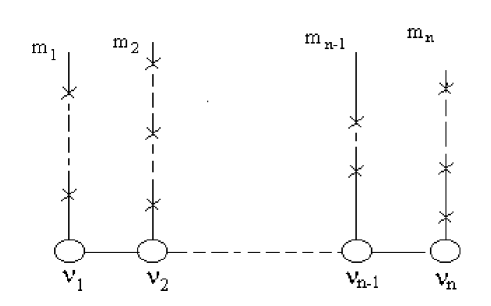
Figure 11: This figure represents a specific FQH system of $n$ parallel layers $\{\mathcal{L}_{a}\}$ with closest interactions. Each layer $\mathcal{L}_{a}$ has $m_{a}$ occupied Landau levels. The filling factor is usually given by a formula type eq(3.53). For layers with different individual filling factors $\nu_{a}$; the symmetry of the model is $U\left(1\right)^{n}$; while for the case where some of the $\nu_{a}$’s are equal, one may have non abelian subgroups of $U\left(n\right)$. More general FQH states involve obviously more complicated simplex.

To that purpose, we start from eq(6.63) describing the effective field model for a single layer hierarchical states and implement the non abelian structure induced from the base B consisting of $n$ $D2$ branes. In the special case where $\left|d_{b}-d_{a}\right|$ goes to zero and moreover all individual hierarchical states of the layers are identical,

$$\mathrm{\nu}_{m_{1}}=\mathrm{\nu}_{m_{2}}=...=\mathrm{\nu}_{m_{n}}=\mathrm{\nu}_{m}$$ (7.1)

one has an exact non abelian $U\left(n\right)$ symmetry and so the NC effective field gauge action follows by substituting the single layer vector bundle $\mathbf{b}_{\mu}$ field by the following $n\times n$ matrix,

$$\mathbf{B}_{\mu}=\sum_{a,b=1}^{n}\mathbf{u}_{ab}\text{ }\mathbf{B}_{\mu}^{ab}$$ (7.2)

where $\mathbf{u}_{ab}$ is as in eq(2.20) and where $\mathbf{B}_{\mu}^{ab}$ are gauge fields connecting layers. These fields are also vectors of the fiber bundle and have the decomposition

$$\mathbf{B}_{\mu}=\sum_{i=1}^{nm}\alpha_{i}\text{ }\mathbf{B}_{\mu}^{i}$$ (7.3)

where $\alpha_{i}$ is the vector basis of the fiber bundle F$\left(B\right)$ based on $\left\{\cup_{a}\mathcal{L}_{a}\right\}$. Taking into account both the decompositions (7.2-3), we can also expand $\mathbf{B}_{\mu}$ as

$$\mathbf{B}_{\mu}=\sum_{a,b=1}^{n}\sum_{i=1}^{nm}\alpha_{i}\text{ }b_{\mu}^{iab}\text{\ }\mathbf{u}_{ab}$$ (7.4)

where $b_{\mu}^{iab}$ are the gauge components on the vector bundle F$\left(\cup_{a=1}^{n}\mathcal{L}_{a}\right)$, see eq(2.19). The generalized intersection matrix extending the single layer matrix of eq(6.1), which correspond to setting $n=m=1$, reads as

$$\alpha_{i}.\alpha_{j}=\widetilde{\mathrm{G}}_{ij};\quad i,j=1,...,nm$$ (7.5)

With these fields and intersection matrix, one can write down the generalized NC effective gauge field model for hierarchical states living on the multilayer system. In the case all layers have the same filling factor, the action of the model has a non abelian $U\left(n\right)$ gauge invariance and reads in terms of the $\mathbf{B}_{\mu}^{i}$ component fields as

$$S\left[\mathbf{B}_{\sigma}^{m},\mathcal{A}_{\mu}^{ex}\right] = \frac{\mathrm{1}}{4\pi}\int d^{3}y\varepsilon^{\mu\nu\sigma}\text{ }\widetilde{\mathrm{G}}_{ij}\mathrm{Tr}_{U\left(n\right)}\left[\mathbf{B}_{\mu}^{i}\ast\partial_{\nu}\mathbf{B}_{\sigma}^{j}+\frac{2i}{3}\widetilde{\mathrm{G}}_{0l}^{-1}\widetilde{\mathrm{G}}_{lk}\text{ }\mathbf{B}_{\mu}^{i}\ast\mathbf{B}_{\nu}^{k}\ast\mathbf{B}_{\sigma}^{j}\right]$$ (7.6)

$$-\frac{\mathrm{1}}{2\pi}\int d^{3}y\varepsilon^{\mu\nu\sigma}\mathrm{Tr}_{U\left(n\right)}\left[\mathbf{q}_{i}.\mathbf{B}_{\mu}^{i}\ast\alpha_{0}\mathbf{\partial}_{\nu}\mathcal{A}_{\sigma}^{ex}\right]$$

Like for eq(6.63), this action may be rewritten in a more condensed form, without using the expansion (7.3), as

$$S\left[\mathbf{B}_{\mu},\mathcal{A}_{\mu}^{ex}\right] = \frac{\mathrm{1}}{4\pi}\int d^{3}y\varepsilon^{\mu\nu\sigma}\mathrm{Tr}_{U\left(n\right)}\left[\mathbf{B}_{\mu}\ast\left(\alpha_{0}\mathbf{\partial}_{\nu}+\frac{2i}{3}\mathbf{\gamma.B}_{\nu}\right)\ast\mathbf{B}_{\sigma}\right]$$ (7.7)

$$-\frac{\mathrm{1}}{2\pi}\int d^{3}y\varepsilon^{\mu\nu\sigma}\mathrm{Tr}_{U\left(n\right)}\left[\mathbf{q}.\mathbf{B}_{\mu}\ast\alpha_{0}\mathbf{\partial}_{\nu}\mathcal{A}_{\sigma}^{ex}\right],$$

where $\mathbf{\partial}_{\nu}$ and $\mathbf{\gamma}$ are as in eqs(6.60-62). Since in the above $U\left(n\right)$ symmetric model, all layer have same individual filling factor $\mathrm{\nu}_{m}$, the total filling factor of this system is,

$$\mathrm{\nu}_{tat}=n\mathrm{\nu}_{m}.$$ (7.8)

It extends naturally the case $\mathrm{\nu}_{tat}=n\mathrm{\nu}_{1}=n/k$ eq(1.4), where all the layers of the system are in the first Landau level; that is of Laughlin type. Along with this $U\left(n\right)$ maximal symmetric situation, one can also derive the other phases of the multilayer system corresponding to the situations where the maximal $U\left(n\right)$ gauge group is broken down to subgroups. Though a little bit cumbersome, these phases are easily computed by following the same lines of the analysis that we have given in sections 3 and 4.

To conclude, we have studied in this paper NC effective field and matrix models for FQH states with rational filling factors. After having given a classification of such states, we have presented our way in handling multilayer and hierarchical states with rational filling factors by using the correspondences: one layer $\mathcal{L}_{a}\longleftrightarrow$ one $D2$ brane and thinking about Landau levels $\left\{{LL}_{i}\right\}$ as fiber bundles on these $D2$ branes; i.e

$$\mathcal{L}_{a} \longleftrightarrow D2\longleftrightarrow{\large B}=\text{Base manifold,}$$

$${LL}_{i} \longleftrightarrow {F}\left(D2\right)\longleftrightarrow{V}=\text{ Fiber bundle}$$ (7.9)

Then, we have studied several representations of FQH states with rational filling factors. These realizations are mainly given by the three following:

(a) Multilayer FQH states where all layers are taken in the first Landau levels. Here we have shown that solutions preserving gauge invariance constraint eqs are specified by the $\left|d_{b}-d_{a}\right|$ distances separating branes; but also by the individual filling factors $\mathrm{\nu}_{a}$. Although the distances $\left|d_{b}-d_{a}\right|$ go to zero $\forall a,b$, $U\left(n\right)$ invariance is not automatic; it requires moreover that all individual filling factors $\mathrm{\nu}_{a}$ have to be equal. This remarkable property has allowed us to distinguish between various kinds of effective fields models; in particular those having abelian gauge symmetries with and without interactions. In section 3, we have studied examples of these solutions and derived new kinds of series, such that

$$\mathrm{\nu}=\frac{k_{1}+k_{2}}{k_{1}k_{2}-l^{2}};\quad k_{1},k_{2}\text{ odd integers,}$$ (7.10)

containing as special cases the level two Jain and Haldane sequences.

This study has also permitted us to shed more light on the varieties of generalizations of Haldane wave functions one encounters in FQH literature. We have taken the opportunity to propose a classification of the generalizations of Laughlin wave function. To our knowledge neither the wave function generalizing the Laughlin wave function with maximal $U\left(n\right)$ gauge symmetry we have obtained in the present study eq(3.61), nor the classification of their generalizations had been known before. Commun results in this matter are naturally covered in our present analysis.

(b) Motivated by the natural correspondence (7.9), we have revisited Wen-Zee effective field model used to describe hierarchical states. First we have shown explicitly that the level of the hierarchy is also the number of the lowest Landau levels $\left\{{LL}_{i}\right\}$ and, as far as Haldane and Jain series are considered, each level of the hierarchy may be though of as described by a kind of Laughlin type state. Though this property is quite manifest on the Jain models; it is however no so obvious for Haldane states. In this regards, we have shown, using an exact mathematical result, that Haldane series may be usually decomposed as a sum over Laughlin type states. To our knowledge such a feature was checked only through specific examples such as $2/5=1/3+1/15$ and $3/7=2/5+1/35$. In subsection 5.3, we have given the exact result to any order; see equations (5.21-24). After having built explicit realizations of Jain and Haldane fiber bundles and shown, amongst others, that Wen-Zee gauge field model follows in straightforward way using fibration ideas, we have studied NC effective field and matrix models extending the Wen-Zee commutative one and recovering the Susskind NC field and Susskind Polychronakos matrix models as special cases.

(c) Combining single layer hierarchy and multilayer states representations, one gets the general situation of FQH fluids. We have also studied this representation and have shown that there are several cases depending on the layers spacings, gauge symmetry and individual filling factors. The most $U\left(n\right)$ symmetric solution one can imagine, has been discussed in the beginning of this section. The general result for subgroups of $U\left(n\right)$ follows naturally from the discussion we have given in this section and the study made in sections 3, 4 and 6.

References

- [1] Leonard Susskind, The Quantum Hall fluid and Noncommutative Chern-Simons Theory. hep-th/0101029.
- [2] Bogdan Morariu, Alexios P. Polychronakos, Finite Noncommutative Chern-Simons with a Wilson Line and the Quantum Hall Effect, hep-th/0106072
- [3] Alexios P. Polychronakos, Quantum Hall states on the cylinder as unitary matrix Chern-Simons theory, hep-th/0106011
- [4] Simeon Hellerman, Mark Van Raamsdonk, Quantum Hall Physics = Noncommutative Field Theory ,hep-th/0103179 Noncommutative Chern-Simons Solitons
- [5] Alexios P. Polychronakos;Quantum Hall states as matrix Chern-Simons theory ; hep-th/0103013; JHEP 0104 (2001) 011.
- [6] Simeon Hellerman, Leonard Susskind; Realizing the Quantum Hall System in String Theory,hep-th/0107200
- [7] Eduardo Fradkin, Vishnu Jejjala and Robert G. Leigh; cond-mat/0205653
- [8] Yuko Kobashi, Bhabani Prasad Mandal, Akio Sugamoto, Exciton in Matrix Formulation of Quantum Hall Effect, hep-th/0202050.
- [9] John H. Brodie (SLAC), L. Susskind, N. Toumbas, How Bob Laughlin Tamed The Giant Graviton From TAUB - NUT SPACE, JHEP 0102:003,2001 and hep-th/0010105
- [10] Dimitra Karabali, Quantum hall Effect in higher dimensions, hep-th/0203264.
- [11] V.P. Nair and A.P. Polychronakos, Phys.Rev.Lett.87:030403,2001, hep-th/0102181.
- [12] Steven S. Gubser, Mukund Rangamani,D-Brane Dynamics and the Qunatum Hall Effect. JHEP 0105:041,2001; hep-th/0012155
- [13] O. Bergman, J. Brodie, Y. Okawa;The Stringy Quantum Hall Fluid, hep-th/0107178
- [14] A.El Rhalami, E.M. Sahraoui, E.H.Saidi; NC Branes and Hierarchies in Quantum Hall Fluids; JHEP 0205 (2002) 004; hep-th/0108096
- [15] Ahmed Jellal, El Hassan Saidi , Hendrik B. Geyer; A Matrix Model for Fractional Quantum Hall States; . hep-th/0204248.
- [16] Michal Fabinger, JHEP 0205 (2002) 037, hep-th/0201016.
- [17] P. A. Horváthy, proceedings of the International Workshop, Nonlinear Physics: Theory and Experiment II. Gallipoli, (Lecce, Italy), to be published by World Scientific. hep-th/0207075
- [18] B. Andrei Bernevig, Chyh-Hong Chern, Jiang-Ping Hu, Nicolaos Toumbas, Shou-Cheng Zhang, Effective field theory description of the higher dimensional quantum Hall liquid, cond-mat/0206164
- [19] Yi-Xin Chen, Bo-Yu Hou, Bo-Yuan Hou, Nucl.Phys. B638 (2002) 220-242, hep-th/0203095
- [20] J.L.F. Barbon, A. Paredes, Noncommutative Field Theory and the Dynamics of Quantum Hall Fluids, hep-th/0112185
- [21] Ana Lopez and Eduardo Fradkin, Universal structure of the edge states of FQH states; cond-mat/9810168
- [22] Joseph Polchinski, String Theory, Cambridge Univ Press 1998.
- [23] Amihay Hanany, Edward Witten, Nucl.Phys. B492 (1997) 152-190, hep-th/9611230.
- [24] L. Feher, L. O’raifeartaigh, P. Ruelle, I. Tsutsui, A. Wipf, On the General Structure of Hamiltonian Reductions of the WZNW Theory; hep-th/9112068.
- [25] V.G. Kac and A.K. Raina, Adv.Ser.Math.Phys.2:1-145,1987;
- [26] E.H. Saidi, M. Zakkari ; Phys.Lett.B281:67-71,1992 and refs therin.
- [27] E.H. Saidi , W A(N-1 / N-1)(1) Miura transformation: Analysis and Applications; IC-92-181, Jul 1992. 46pp.
- [28] Niclas Wyllard, Nucl.Phys.B491:461-476,1997, hep-th/9609125 .
- [29] X.G. Wen and A. Zee ,Phys.Rev.B46(1992)2290.
- [30] X.G. Wen, Adv.Phys.44,405, (1995).
- [31] Xiao-Gang Wen, Topological Orders and Edge Excitations in FQH States. PRINT-95-148, (MIT),cond-mat/9506066.
- [32] I. Benkaddour, A. EL Rhalami, E.H. Saidi :Eur.Phys.J. C21 (2001) 735-747, hep-th/0007142.
- [33] Safi Bahcall and Leonard Susskind , Fluid Dynamics, Chern-Simons Theory and the Quantum Hall Effect; Int.J.Mod.Phys.B5:2735-2750,1991 35
- [34] S. Katz, P. Mayr and C. Vafa; Adv.Theor.Math.Phys.1:53-114,1998, hep-th/9706110.
- [35] A. Belhaj, A. Elfallah, E.H. Saidi; Class.Quant.Grav.16:3297-3306,1999; Class.Quant.Grav.17:515-532,2000; : hep-th/0012131 .
-
[36]
R.B.Laughlin, Phys.rev.Lett. 50(1983)1395.
- [37] E.Fradkin, Field Theories of Condensed Matter Systems, Lecture Note Series V82(1991)
- [38] D.Arovas, J.R.Schrieffer and F.Wilczek: Fractional Statistics in the Quantum Hall Effect,Phys.Rev.Lett.53(1984)722-723;
- [39] N.Read,Phys.Rev.Lett. 65,(1990)1502.
- [40] R.E.Prange and S.M. Girvin, The Quantum Hall effect(Springer, New York, 1987).
- [41] Hendrik.B.Geyer; Field Theory, Topology and Condensed matter Physics,Proceedings of the Ninth Chris Engelbrecht Summer School in theoretical Physics. Held at:Storms River Mouth, Tsitsikamma National Parkc, South africa, 17-28 January 1994.Springer 1995. (see) A.Zee,Quatum Hall Fluid
- [42] Steven M. Girvin,(Indiana University), ”The Quantum Hall Effect: Novel Excitations and Broken Symmetries”,cond-mat/9907002.
- [43] L Susskind; Letures given at the workshop on String theory and Quantum Gravity (2002), Stellenbosch; South Africa.
- [44] Dongsu Bak, Sung Ku Kim, Kwang-Sup Soh, Jae Hyung Yee Phys.Rev. D64 (2001) 025018
- [45] Avinash Khare, M. B.Paranjape, JHEP 0104 (2001) 002
- [46] Alexios P. Polychronakos, JHEP 0106 (2001) 070, hep-th/0106011.
- [47] R. Jackiw, S.-Y. Pi, A.P. Polychronakos, hep-th/0206014.
- [48] I. Benkaddour, A. EL Rhalami, E.H. Saidi :Fractional Quantum Hall Excitations as RdTS Highest Weight State, hep-th/0101188
- [49] Ben Freivogel, Leonard Susskind, Nicolaos Toumbas, A Two Fluid Description of the Quantum Hall Soliton, hep-th/0108076.
- [50] Ahmed Jellal, Hendrik B. Geyer; hep-th/0201203.
- [51] Dimitra Karabali, Bunji Sakita, Phys.Rev. B64 (2001) 245316, Phys.Rev. B65 (2002) 075304.
- [52] O.F. Dayi, A. Jellal; Phys.Lett. A287 (2001) 349-355; cond-mat/0103562.
- [53] Dimitra Karabali, V.P. Nair, Quantum Hall Effect in Higher Dimensions; hep-th/0203264.
- [54] N.Seiberg and E.Witten, JHEP 9909:032,1999, hep-th/9908142
- [55] J.K. Jain; Phys Rev Lett 63 (1989) 199.
- [56] D.M. Haldane, Fractional Quantization of the Hall Effect: A Hierarchy of Incompressible Quantum Fluid States. Phys.Rev.Lett.51:605-608,1983.