CERN-TH/2002-196

hep-th/0208141

Notes on Orientifolds of Rational Conformal Field Theories
Ilka Brunner^∗ and Kentaro Hori^†

^∗Theory Division, CERN, CH-1211 Geneva 23, Switzerland
^†Institute for Advanced Study, Princeton, New Jersey 08540, U.S.A.
and
University of Toronto, Toronto, Ontario M5S 1A7, Canada

We review and develop the construction of crosscap states associated with parity symmetries in rational conformal field theories. A general method to construct crosscap states in abelian orbifold models is presented. It is then applied to rational $U(1)$ and parafermion systems, where in addition we study the geometrical interpretation of the corresponding parities.

CERN-TH/2002-196

August 2002

1 Introduction

Four-dimensional string compactifications with ${\mathcal{N}}=1$ supersymmetry allowing non-abelian gauge symmetries and chiral matter contents are phenomenologically appealing. Recently, D-branes on Calabi–Yau threefolds were studied extensively, partly because one may obtain ${\mathcal{N}}=1$ supersymmetry in four dimensions if the D-branes extend in the dimensions transverse to the Calabi-Yau. However, consistency conditions require either the Calabi–Yau to be non-compact or the tadpoles to be cancelled by some other objects. In the former case, we are left with four-dimensional theories where gravity is essentially decoupled. Although such systems are interesting in their own right, our main concern is the theory in four dimensions with a finite Newton’s constant. Thus, we need to consider compact internal spaces. The only known candidates to cancel the tadpoles while maintaining ${\mathcal{N}}=1$ supersymmetry are orientifold planes.

Orientifolding means to gauge a parity symmetry of the worldsheet theory. The basic example is the gauging of the worldsheet orientation reversal $\Omega$ of the Type IIB superstring, resulting in the Type I superstring. One is free, however, to consider more general parity actions where $\Omega$ is combined with some action on space-time with a necessary consistency condition that this combination is a symmetry of the underlying theory [2, 3, 4, 5, 6] (see [7] for a recent review). The fixed-point sets of the space-time action, called orientifold planes, can carry tension and RR charges opposite to those of D-branes and can be used for tadpole cancellation. A crosscap state is associated to each parity symmetry, just as a boundary state is associated with a boundary condition or D-brane [8, 9]. These crosscap states encode the physical data, such as tension and RR charges of the orientifold planes.

One approach to study orientifolds of Calabi–Yau manifolds is to consider special points in the moduli space where the worldsheet theory is exactly solvable. One class of such models are toroidal orbifolds, which have been extensively studied [10, 11, 12]. Another important class of systems are Gepner models whose basic building blocks are rational ${\mathcal{N}}=2$ superconformal field theories (see [13, 14] for earlier work on orientifolds of Gepner models). However, general methods to study parity symmetries and orientifolds of such models are not developed to the same extent as in the case of D-branes.

The purpose of the present paper is to collect and review the known techniques to study orientifolds of rational conformal field theories (RCFTs) and further develop them. We present a coherent method to construct parity symmetries and the corresponding crosscap states in RCFTs and their orbifolds. The method is then applied to two simple examples, the rational $U(1)$ and the parafermions $SU(2)/U(1)$. This serves as a warm-up to the ${\mathcal{N}}=2$ models, which will be reported in a forthcoming paper [15]. Along the way, we also find the geometrical interpretation of the parity symmetries of these examples.

In Section 2 we describe boundary and crosscap states and the corresponding parities in RCFTs. We review the construction of a universal crosscap state by Pradisi–Sagnotti–Stanev (PSS) [16], which applies in any RCFT with the charge conjugation modular invariant. The corresponding parities can be combined with the discrete symmetries of the system, giving rise to the class of crosscap states considered in [17]. These crosscap states, as well as the rational boundary states constructed by Cardy, preserve the diagonal subalgebra ${\cal A}$ of the full symmetry algebra ${\cal A}\otimes{\cal A}$.

We then proceed to study parity symmetries of orbifold models and provide a general new method to construct the crosscap states. The emerging picture is much cleaner than the construction of boundary states, which suffers from the fixed-point resolution problem. Our method can be used to explain the result of an earlier paper [18], which also studied the same subject (see [19, 20] for earlier work concerning various special cases).

In the last subsection, we consider D-branes and parities preserving the subalgebra ${\cal A}$ embedded into the symmetry algebra ${\cal A}\otimes{\cal A}$ through an automorphism $\omega$ of ${\cal A}$: $W\mapsto A\otimes 1+1\otimes\omega(W)$, in particular the mirror automorphism that acts as charge conjugation. Extending the terminology of the ${\mathcal{N}}=2$ supersymmetry algebra [21, 15], we call them B-branes/B-parities while the ones preserving the ordinary diagonal subalgebra shall be called A-branes/A-parities. Sometimes, an orbifold model is the mirror of the original model. In such cases, B-branes and B-parities can be obtained by applying the mirror map to A-branes/A-parities of the mirror, which are constructed using orbifold techniques.

Sections 3, 4, 5 and 6 are devoted to examples. In Section 3 we revisit the free boson compactified on a circle of arbitrary radius, including an extension of the standard construction [8, 9] to non-involutive parities. We prove that the orientifold corresponding to the parity where the target space action consists of a half-period shift of the circle is T-dual to the orientifold associated to the reflection $X\rightarrow-X$ of the circle coordinate with one $SO$- and one $Sp$-type orientifold plane (see [7] for a recent related discussion). Section 4 is concerned with the special case that the radius of the circle is $R=\sqrt{k}$, $k$ a positive integer. In this case, the theory becomes rational and one can apply the method of Section 2. It is instructive to see how the RCFT data encodes geometrical and physical information of the orientifolds in this simple case.

Our second example is the parafermion system, which is discussed in Sections 5 and 6. This model has a lagrangian description in terms of a $SU(2)_{k}$ mod $U(1)_{k}$ gauged WZW model that is particularly well adapted to a study of the geometrical interpretation of parity actions. Geometrically, the parafermion theory can be understood as a sigma-model with a disk target space parametrized by a complex coordinate $z$ with $|z|\leq 1$. D-branes in this model have been studied in [22]. A-type parities act as antiholomorphic involutions of the target geometry, the basic example being $z\rightarrow\bar{z}$. It is possible to combine this with an element of the ${\bf Z}_{k}$ symmetry of the theory, which acts as a phase multiplication on the target space coordinate. Accordingly, the corresponding orientifold planes are located along diameters of the disk. B-type parities act holomorphically on the target space, the fundamental B-type parity being $z\rightarrow z$. This involution leaves the whole disk fixed and therefore corresponds to an orientifold 2-plane. Combining this with phase rotations leads generically to non-involutive parities, which we also consider. In the case where the level $k$ of the parafermion theory is even, there is a second involutive parity, $z\rightarrow-z$, which leaves only the center of the disk fixed and hence describes an orientifold 0-plane. Finally we discuss the same model purely in terms of rational conformal field theory and give a detailed map of RCFT results to geometrical properties. The questions discussed in Section 6 have been partially addressed in [23], but we disagree with some of the results in that paper. In particular, we find that the geometric interpretation of the PSS crosscap states is different.

2 Crosscaps in RCFT

We begin by describing the construction of boundary and crosscap states of rational conformal field theories. A review and extension of previous work in [24, 25, 16, 17, 18, 26, 27, 28, 29] is followed by developing new techniques to construct crosscap states in orbifolds.

We consider a quantum field theory in $1+1$ dimensions. Let ${\mathcal{H}}_{g}$ be the space of states of the system formulated on a circle with the $g$-twisted periodic boundary condition, where $g$ is an internal symmetry. Let ${\mathcal{H}}_{\alpha_{1},\alpha_{2}}$ be the space of states on a segment with the boundary conditions $\alpha_{1}$ and $\alpha_{2}$ at the left and the right ends. We denote by $|\Scr{B}_{\alpha}\rangle$ and $|\Scr{C}_{P}\rangle$ the boundary and crosscap states corresponding to a boundary condition $\alpha$ and a parity symmetry $P=\tau\Omega$ . The cylinder, Klein bottle (KB), and Möbius strip (MS) amplitudes are expressed in two ways

$${\rm Tr}\!\!\mathop{}_{{\mathcal{H}}_{\alpha_{1},\alpha_{2}}}g\,{\rm e}^{-\beta H_{o}(L)}=\mathop{}_{g}\!\langle\Scr{B}_{1}|\,{\rm e}^{-LH_{c}(\beta)}|\Scr{B}_{2}\rangle\!\!\mathop{}_{g},$$ (2.1)

$${\rm Tr}\!\!\mathop{}_{{\mathcal{H}}_{P_{1}P_{2}^{-1}}}\!\!P_{2}\,{\rm e}^{-\beta H_{c}(L)}=\langle\Scr{C}_{1}|\,{\rm e}^{-{L\over 2}H_{c}(2\beta)}|\Scr{C}_{2}\rangle,$$ (2.2)

$${\rm Tr}\!\!\mathop{}_{{\mathcal{H}}_{\alpha,P(\alpha)}}\!\!P\,{\rm e}^{-\beta H_{o}(L)}=\mathop{}_{P^{2}}\!\langle\Scr{B}_{\alpha}|\,{\rm e}^{-{L\over 2}H_{c}(2\beta)}|\Scr{C}_{P}\rangle.$$ (2.3)

Here $H_{c}(\ell)$ and $H_{o}(\ell)$ are the Hamiltonians of the system on a circle of circumference $\ell$ and segment of length $\ell$ respectively. (The Hilbert spaces and boundary/crosscap states also depend on the lengths which are omitted for notational simplicity.) The subscripts of the boundary states show the periodicity of the boundary circle. For instance, $|\Scr{B}_{2}\rangle_{g}$ consists of elements in ${\mathcal{H}}_{g}$. Note that $|\Scr{C}_{P}\rangle$ has a periodicity determined by $P^{2}$. (Eq (2.2) makes sense only if $P_{1}^{2}=P_{2}^{2}$.) In (2.3), $P(\alpha)$ stands for the $P$-image of the boundary condition $\alpha$. The left and the right hand sides of (2.1)–(2.3) may be referred to as loop channel and tree channel expressions respectively.

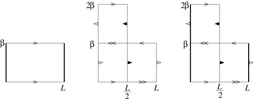
Figure 1: Cylinder, Klein Bottle and Möbius Strip

In what follows, we will consider conformally invariant quantum field theories and study boundary conditions and parity symmetries that preserve the conformal invariance. In such a theory, one can rescale the lengths $(L,\beta)\rightarrow(\lambda L,\lambda\beta)$ without changing the amplitudes. It is customary to choose the circumference of the closed string to be $2\pi$ and the length of the open string to be $\pi$. Suppose we choose $(L,\beta)=(\pi,-2\pi i\tau),(2\pi,-2\pi i\tau),(\pi,-2\pi i\tau)$ in the loop channel expressions of (2.1), (2.2), (2.3) respectively, where $\tau$ is a complex number on the positive imaginary axis. Then in the tree-channel expressions, we take $(L,\beta)=(-\pi i/\tau,2\pi),(-\pi i/\tau,\pi),(-\pi i/2\tau,\pi)$. In string theory, Eqs. (2.1)-(2.3) are referred to as loop/tree channel duality and have played an important role (see e.g. [10]).

The System We Consider

We consider an RCFT based on a chiral algebra ${\mathcal{A}}=\{W_{n}^{(r)}\}$ with a set of representations $\{\Scr{H}_{i}\}$. We primarily consider the model ${\mathcal{C}}$ with the Hilbert space of states

$${\mathcal{H}}^{\mathcal{C}}=\bigoplus_{i}\Scr{H}_{i}\otimes\Scr{H}_{\overline{\imath}}.$$ (2.4)

where $\overline{\imath}$ is the BPZ conjugate of $i$. This model has ${\mathcal{A}}\otimes{\mathcal{A}}$ symmetry algebra generated by $W^{(r)}=W^{(r)}\otimes 1$ and $\widetilde{W}^{(r)}=1\otimes W^{(r)}$. For each representation $i$, we fix an antiunitary operator $U:\Scr{H}_{i}\rightarrow\Scr{H}_{\overline{\imath}}$ such that

$$UW_{n}^{(r)}U^{-1}=(-1)^{s_{r}}{W_{-n}^{(r)}}^{{\dagger}}\quad\forall r,$$ (2.5)

where $s_{r}$ is a spin of the current $W^{(r)}$.

2.1 Symmetry-Preserving D-branes/Orientifolds

We first study D-branes and orientifolds that preserve a diagonal subalgebra of the ${\mathcal{A}}\otimes{\mathcal{A}}$ symmetry. On the Minkowski worldsheet with time and space coordinates $(t,x)$, “symmetry-preserving” means the following: for D-branes the associated boundary conditions (say, at $x=0$) are such that $W^{(r)}(t,0)=\widetilde{W}^{(r)}(t,0)$, while orientifolds should be associated with parity symmetries that map $W^{(r)}(t,x)$ to $\widetilde{W}^{(r)}(t,-x)$.

2.1.1 Constraints on Boundary/Crosscap Coefficients

A Wick rotation followed by a 90^∘ rotation show that the boundary and crosscap states obey

$$(W^{(r)}_{n}-(-1)^{s_{r}}\widetilde{W}^{(r)}_{-n})|\Scr{B}\rangle=0,$$ (2.6)

$$(W^{(r)}_{n}-(-1)^{s_{r}+n}\widetilde{W}^{(r)}_{-n})|\Scr{C}\rangle=0.$$ (2.7)

The basic set of solutions to these equations was found by Ishibashi [25]. Let us denote by $\{|i,N\rangle\}_{N}$ an orthonormal basis of the representation $\Scr{H}_{i}$. Equations (2.6) and (2.7) are solved respectively by

$$|\Scr{B},i\rangle\!\rangle:=\sum_{N}|i,N\rangle\otimes U|i,N\rangle,$$ (2.8)

$$|\Scr{C},i\rangle\!\rangle:=\,{\rm e}^{\pi i(L_{0}-h_{i})}|\Scr{B},i\rangle\!\rangle.$$ (2.9)

It follows from the definition that

$$\langle\!\langle\Scr{B},i|\,{\rm e}^{2\pi i\tau H_{c}}|\Scr{B},j\rangle\!\rangle=\delta_{i,j}\chi_{i}(2\tau),$$ (2.10)

$$\langle\!\langle\Scr{C},i|\,{\rm e}^{2\pi i\tau H_{c}}|\Scr{C},j\rangle\!\rangle=\delta_{i,j}\chi_{i}(2\tau),$$ (2.11)

$$\langle\!\langle\Scr{B},i|\,{\rm e}^{2\pi i\tau H_{c}}|\Scr{C},j\rangle\!\rangle=\delta_{i,j}\widehat{\chi}_{i}(2\tau),$$ (2.12)

where $H_{c}=L_{0}+\widetilde{L}_{0}-c/12$ and $\widehat{\chi}_{i}(\tau)=\,{\rm e}^{-\pi i(h_{i}-c/24)}\chi_{i}(\tau+{1\over 2})$. The actual boundary and crosscap states are linear combinations of these Ishibashi-states:

$$|\Scr{B}_{\alpha}\rangle=\sum_{i}n_{\alpha i}|\Scr{B},i\rangle\!\rangle,$$ (2.13)

$$|\Scr{C}_{\mu}\rangle=\sum_{i}\gamma_{\mu i}|\Scr{C},i\rangle\!\rangle.$$ (2.14)

Here $\alpha$ and $\mu$ are the labels for the boundary conditions and parity symmetries. We first assume that the parity symmetries are involutive $P_{\mu}^{2}=1$. (We will later treat those that are not involutive.) A set of constraints on the coefficients $n_{\alpha b}$ and $\gamma_{\mu b}$ are found by using the loop/tree channel duality (2.1)–(2.3):

$${\rm Tr}\!\!\mathop{}_{{\mathcal{H}}_{\alpha,\beta}}\!\,{\rm e}^{2\pi i\tau H_{o}}=\langle\Scr{B}_{\alpha}|\,{\rm e}^{-{\pi i\over\tau}H_{c}}|\Scr{B}_{\beta}\rangle,$$ (2.15)

$${\rm Tr}\!\!\mathop{}_{{\mathcal{H}}_{g_{\mu\nu}}}\!\!P_{\nu}\,{\rm e}^{2\pi i\tau H_{c}}=\langle\Scr{C}_{\mu}|\,{\rm e}^{-{\pi i\over 2\tau}H_{c}}|\Scr{C}_{\nu}\rangle,$$ (2.16)

$${\rm Tr}\!\!\mathop{}_{{\mathcal{H}}_{\alpha,\mu(\alpha)}}\!\!P_{\mu}\,{\rm e}^{2\pi i\tau H_{o}}=\langle\Scr{B}_{\alpha}|\,{\rm e}^{-{\pi i\over 4\tau}H_{c}}|\Scr{C}_{\mu}\rangle,$$ (2.17)

where $g_{\mu\nu}$ is the internal symmetry $P_{\mu}P_{\nu}^{-1}$ that commutes with the chiral algebra ${\mathcal{A}}\otimes{\mathcal{A}}$, and $\mu(\alpha)$ is the $P_{\mu}$-image of the boundary condition $\alpha$.

Since the diagonal symmetry ${\mathcal{A}}$ is preserved by the boundary conditions $\alpha$ and $\beta$, open string states fall into a sum of irreducible representations

$${\mathcal{H}}_{\alpha,\beta}=\bigoplus_{i}n_{\alpha\beta}^{i}\Scr{H}_{i}$$ (2.18)

on which $H_{o}$ acts as $L_{0}-{c\over 24}$, where $n_{\alpha\beta}^{i}$ are non-negative integers. Using (2.10), (2.15) is expressed as

$$\sum_{i}n_{\alpha\beta}^{i}\chi_{i}(\tau)=\sum_{i}n_{\alpha i}^{*}n_{\beta i}\chi_{i}(-1/\tau).$$ (2.19)

For a symmetry $g$ that commutes with the chiral algebra ${\mathcal{A}}\otimes{\mathcal{A}}$, the space ${\mathcal{H}}_{g}$ of $g$-twisted closed string states can be decomposed into the representations of ${\mathcal{A}}\otimes{\mathcal{A}}$,

$${\mathcal{H}}_{g}=\bigoplus_{ij}h^{ij}_{g}\Scr{H}_{i}\otimes\Scr{H}_{j},$$ (2.20)

where $h^{ij}_{g}$ are non-negative integers. Note that $P_{\nu}$ transforms the $g$-twisted boundary condition into the $\tau_{\nu}g^{-1}\tau_{\nu}^{-1}$-twisted boundary condition. Since $P_{\nu}$ is a symmetry-preserving parity, $P_{\nu}W_{n}^{(r)}=\widetilde{W}_{n}^{(r)}P_{\nu}$, it acts on the closed string states essentially by the exchange of the left and right factors. To be more precise, it maps the subspace $h^{ij}_{g}\Scr{H}_{i}\otimes\Scr{H}_{j}$ of ${\mathcal{H}}_{g}$ to a subspace of ${\mathcal{H}}_{\tau_{\nu}g^{-1}\tau_{\nu}^{-1}}$ as

$$P_{\nu}:\xi\otimes u\otimes v\in{\bf C}^{h^{ij}_{g}}\otimes\Scr{H}_{i}\otimes\Scr{H}_{j}\mapsto K_{\nu}^{ij}(g)\xi\otimes v\otimes u\in{\bf C}^{h^{ji}_{\tau_{\nu}g^{-1}\tau_{\nu}^{-1}}}\otimes\Scr{H}_{j}\otimes\Scr{H}_{i},$$ (2.21)

where $K_{\nu}^{ij}(g)$ is a matrix acting on the multiplicity space ${\bf C}^{h^{ij}_{g}}\cong{\bf C}^{h^{ji}_{\tau_{\nu}g^{-1}\tau_{\nu}^{-1}}}$. (Note that it has to be the case that $h^{ij}_{g}=h^{ji}_{\tau_{\nu}g^{-1}\tau_{\nu}^{-1}}$.) $P_{\nu}^{2}=1$ requires $K_{\nu}^{ji}(\tau_{\nu}g^{-1}\tau_{\nu}^{-1})K_{\nu}^{ij}(g)=1$. In particular, $K_{\nu}^{ii}(g_{\mu\nu})$ is a matrix that squares to 1 and therefore its eigenvalues must be $\pm 1$. Thus, using (2.11), (2.16) is expressed as

$$\sum_{i}k_{\mu\nu}^{i}\chi_{i}(2\tau)=\sum_{i}\gamma_{\mu i}^{*}\gamma_{\nu i}\chi_{i}(-1/2\tau),$$ (2.22)

where $k_{\mu\nu}^{i}={\rm tr}K_{\nu}^{ii}(g_{\mu\nu})$. Since $K_{\nu}^{ii}(g_{\mu\nu})$ squares to $1$, the number $k_{\mu\nu}^{i}$ must be an integer such that $|k_{\mu\nu}^{i}|\leq h^{ii}_{g_{\mu\nu}}$ and $k_{\mu\nu}^{i}\equiv h^{ii}_{g_{\mu\nu}}$ mod 2.

Let us next consider the action of $P_{\mu}$ on open string states. Since it exchanges the left and right boundaries of the string, the symmetry-preserving condition becomes $P_{\mu}W_{n}^{(r)}=(-1)^{n}W_{n}^{(r)}P_{\mu}$. It therefore has to transform the subspace $\Scr{H}_{i}^{\oplus n_{\alpha\beta}^{i}}$ of ${\mathcal{H}}_{\alpha,\beta}$ to a subspace of ${\mathcal{H}}_{\mu(\beta),\mu(\alpha)}$ as

$$P_{\mu}:\eta\otimes u\in{\bf C}^{n_{\alpha\beta}^{i}}\otimes\Scr{H}_{i}\mapsto M_{\alpha\beta,\mu}^{i}\eta\otimes\,{\rm e}^{\pi i(L_{0}-h_{a})}u\in{\bf C}^{n_{\mu(\beta)\mu(\alpha)}^{i}}\otimes\Scr{H}_{i},$$

where $M_{\alpha\beta,\mu}^{i}$ is a matrix acting on ${\bf C}^{n_{\alpha\beta}^{i}}$. (Note that $n_{\alpha\beta}^{i}$ must be equal to $n_{\mu(\beta)\mu(\alpha)}^{i}$ for any $i$.) $P_{\mu}^{2}=1$ requires $M_{\mu(\beta)\mu(\alpha)}^{i}M_{\alpha\beta,\mu}^{i}=1$. In particular, the eigenvalues of the matrix $M_{\alpha\mu(\alpha)}^{i}$ have to be $\pm 1$. Using this, we can rewrite (2.17) as

$$\sum_{i}m_{\alpha,\mu}^{i}\widehat{\chi}_{i}(\tau)=\sum_{i}n_{\alpha i}^{*}\gamma_{\mu i}\widehat{\chi}_{i}(-1/4\tau),$$ (2.23)

where $m_{\alpha\mu}^{i}={\rm tr}M_{\alpha\mu(\alpha),\mu}^{i}$. For $P_{\mu}^{2}=1$, the number $m_{\alpha\mu}^{i}$ must be an integer such that $\pm m_{\alpha\mu}^{i}\leq n_{\alpha\mu(\alpha)}^{i}$ and $m_{\alpha\mu}^{i}\equiv n_{\alpha\mu(\alpha)}^{i}$ mod 2.

We have found the constraints (2.19), (2.22) and (2.23). At this stage, we use the modular transformation property of characters

$$\chi_{j}(-1/\tau)=\sum_{i}\chi_{i}(\tau)S_{ij},$$

$$\chi_{j}(\tau+1)=\sum_{i}\chi_{i}(\tau)T_{ij},$$

$$\widehat{\chi}_{j}(-1/4\tau)=\sum_{i}\widehat{\chi}_{i}(\tau)P_{ij},$$

where

$$P=\sqrt{T}ST^{2}S\sqrt{T},$$ (2.24)

in which $\sqrt{T}_{ij}=\delta_{i,j}\,{\rm e}^{\pi i(h_{i}-{c\over 24})}$. Here we are in the standard convention, $STS=T^{-1}ST^{-1}$. The three constraints can then be rewritten as

$$n_{\alpha\beta}^{i}=\sum_{j}n_{\alpha j}^{*}n_{\beta j}S_{ij},$$ (2.25)

$$k_{\mu\nu}^{i}=\sum_{j}\gamma_{\mu j}^{*}\gamma_{\nu j}S_{ij},$$ (2.26)

$$m_{\alpha\mu}^{i}=\sum_{j}n_{\alpha j}^{*}\gamma_{\mu j}P_{ij},$$ (2.27)

where $n_{\alpha\beta}^{i}$, $k_{\mu\nu}^{i}$ and $m_{\alpha\mu}^{i}$ are integers such that

$$\begin{array}[]{l}\bullet\,\,\,\,n_{\alpha\beta}^{i}\geq 0,\\ \bullet\,\,\,\,-h^{ii}_{g_{\mu\nu}}\leq k_{\mu\nu}^{i}\leq h^{ii}_{g_{\mu\nu}},\quad k_{\mu\nu}^{i}\equiv h^{ii}_{g_{\mu\nu}}\,\,(\mbox{mod 2}),\\ \bullet\,\,\,\,-n_{\alpha\mu(\alpha)}^{i}\leq m_{\alpha\mu}^{i}\leq n_{\alpha\mu(\alpha)}^{i},\quad m_{\alpha\mu}^{i}\equiv n_{\alpha\mu(\alpha)}^{i}\,\,(\mbox{mod 2}),\\ \end{array}$$ (2.28)

where $h_{g}^{ij}$ is the multiplicity of $\Scr{H}_{i}\otimes\Scr{H}_{j}$ in the space ${\mathcal{H}}_{g}$ of the $g$-twisted closed string states.

2.1.2 Cardy–PSS Solution

A simple solution to the above constraints that applies to all RCFTs has been found by Cardy [24] for boundary states and by Pradisi–Sagnotti–Stanev [16] for a crosscap state.

Cardy’s boundary conditions carry the same labels as the representations $\{i\}$. The coefficients $n_{ij}$ and the multiplicities $n_{ij}^{k}$ are given in terms of the modular $S$-matrix and the fusion coefficients:

$$n_{ij}={S_{ij}\over\sqrt{S_{0j}}},$$ (2.29)

$$n_{ij}^{k}=N_{\overline{\imath}j}^{\overline{k}}.$$ (2.30)

The constraints (2.25) translate into the Verlinde formula [30].

PSS have found a crosscap state that corresponds to a parity symmetry transforming the Cardy boundary states as

$$P_{0}:i\mapsto\overline{\imath}.$$ (2.31)

We label this state by “0” for a reason that will become clear shortly. The coefficients $\gamma_{0i}$ and the numbers $k_{00}^{i}$, $m_{i0}^{j}$ are given by

$$\gamma_{0i}={P_{0i}\over\sqrt{S_{0i}}},$$ (2.32)

$$k_{00}^{i}=Y_{i0}^{0},$$ (2.33)

$$m_{i0}^{j}=Y_{\overline{\imath}0}^{\overline{\jmath}},$$ (2.34)

where $Y_{ij}^{k}$ is defined by

$$Y_{ij}^{k}=\sum_{l}{S_{il}P_{jl}P_{kl}^{*}\over S_{0l}}.$$ (2.35)

It is straightforward to show that the constraints (2.26) and (2.27) are satisfied for the PSS crosscap state. To see that they obey (2.28), we first note that $g_{00}=1$ and therefore $h^{ii}_{g_{00}}=h^{ii}=\delta_{i,\overline{\imath}}$ because ${\mathcal{H}}_{1}={\mathcal{H}}=\oplus_{i}\Scr{H}_{i}\otimes\Scr{H}_{\overline{\imath}}$. The conditions (2.28) therefore require $k_{00}^{i}=\pm\delta_{i,\overline{\imath}}$. Also, since $n_{iP(i)}^{j}=n_{i\overline{\imath}}^{j}=N_{\overline{\imath}\overline{\imath}}^{\overline{\jmath}}$, the number $m_{i0}^{j}$ must be an integer such that $|m_{i0}^{j}|\leq N_{\overline{\imath}\overline{\imath}}^{\overline{\jmath}}$ and $m_{i0}^{j}\equiv N_{\overline{\imath}\overline{\imath}}^{\overline{\jmath}}$ (mod 2). These constraints are obeyed by the above solution because of

Bantay’s Relation [27]

$$\begin{array}[]{l}|Y_{i0}^{j}|\leq N_{ii}^{j},\\ Y_{i0}^{j}\equiv N_{ii}^{j}\quad\mbox{mod 2}.\end{array}$$ (2.36)

Indeed the condition on $m_{i0}^{j}=Y_{\overline{\imath}0}^{\overline{\jmath}}$ is nothing but Bantay’s relation. The condition on $k_{00}^{i}=Y_{i0}^{0}$ also follows from this since $N_{ii}^{0}=\delta_{i,\overline{\imath}}$.

The number $Y_{i0}^{0}$ (which is $\pm 1$ if $i=\overline{\imath}$ and 0 otherwise) is a CFT analog of the Frobenius–Schur indicator for the theory of group representations .

2.1.3 Dressing by Discrete Symmetries

If an RCFT has a discrete symmetry of a certain type, one can find additional parity symmetries together with the corresponding crosscap states.

Let $\Scr{G}$ be the finite abelian group generated by the simple currents $\{g\}$. We recall that a simple current $g$ is a representation such that the fusion product of $g$ with any representation $i$ contains only one representation, which we denote by $g(i)$. Let us introduce the number

$$Q_{g}(i)=h_{i}+h_{g}-h_{g(i)}\quad\mbox{mod 1}.$$ (2.37)

The map $g\mapsto\,{\rm e}^{2\pi iQ_{g}(i)}$ defines for each $i$ a homomorphism $\Scr{G}\rightarrow U(1)$ (some of the properties of $Q_{g}(i)$ are summarized in Appendix B). We can thus define a representation of $\Scr{G}$ on the Hilbert space ${\mathcal{H}}$ in such a way that $g$ acts by the phase multiplication $\,{\rm e}^{2\pi iQ_{g}(i)}\times$ on the subspace $\Scr{H}_{i}\otimes\Scr{H}_{\overline{\imath}}$. The Cardy state $|\Scr{B}_{i}\rangle$ is mapped by $g$ as

$$|\Scr{B}_{i}\rangle=\sum_{j}{S_{ij}\over\sqrt{S_{0j}}}|\Scr{B},j\rangle\!\rangle\stackrel{{\scriptstyle g}}{{\mapsto}}\sum_{j}{S_{ij}\over\sqrt{S_{0j}}}\,{\rm e}^{2\pi iQ_{g}(j)}|\Scr{B},j\rangle\!\rangle=\sum_{j}{S_{g(i)j}\over\sqrt{S_{0j}}}|\Scr{B},j\rangle\!\rangle=|\Scr{B}_{g(i)}\rangle,$$ (2.38)

where we have used $S_{g(i)j}=\,{\rm e}^{2\pi iQ_{g}(j)}S_{ij}$.

We now find new parity symmetries $P_{g}$ that act on ${\mathcal{H}}$ as $g\circ P_{0}$. It follows from (2.31) and (2.38), that these parities should map the Cardy branes as

$$P_{g}:i\mapsto g(\overline{\imath}).$$ (2.39)

The crosscap coefficients and the numbers $k_{g_{1}g_{2}}^{i}$, $m_{ig}^{j}$ are given by

$$\gamma_{gi}={P_{gi}\over\sqrt{S_{0i}}},$$ (2.40)

$$k_{g_{1}g_{2}}^{i}=Y_{ig_{2}}^{g_{1}}$$ (2.41)

$$m_{ig}^{j}=Y_{\overline{\imath}g}^{\overline{\jmath}}.$$ (2.42)

It is easy to show that this solves the constraints (2.26) and (2.27) [16, 17]. The Y-tensors can be rewritten as

$$Y_{ig_{2}}^{g_{1}}=\,{\rm e}^{\pi i(\hat{Q}_{g_{2}}(g_{2}^{-1}g_{1})-2Q_{g_{2}}(i))}Y_{i0}^{g_{2}^{-1}g_{1}},\quad Y_{\overline{\imath}g}^{\overline{\jmath}}=\,{\rm e}^{\pi i(\hat{Q}_{g}(g^{-1}(\overline{\jmath}))-2Q_{g}(\overline{\imath}))}Y_{\overline{\imath}0}^{g^{-1}(\overline{\jmath})},$$ (2.43)

where $\hat{Q}_{g}(i):=h_{i}+h_{g}-h_{g(i)}$ (not just modulo integers). Since $\,{\rm e}^{\pi i(\hat{Q}_{g}(b)-2Q_{g}(a))}=\pm 1$ if $Y_{a0}^{b}\neq 0$, the integrality of $k_{g_{1}g_{2}}^{i}$ and $m_{ig}^{j}$ is also satisfied.

In order to show that the last constraint (2.28) is satisfied, we need to find the multiplicities $h_{g_{12}}^{ii}$ and $n_{iP_{g}(i)}^{j}$, where $g_{12}=P_{1}P_{2}^{-1}=g_{1}g_{2}^{-1}$ and $P_{g}(i)=g(\overline{\imath})$ by (2.39). The space of $g$-twisted closed string states is given by ${\mathcal{H}}_{g}=\oplus_{i}\Scr{H}_{i}\otimes\Scr{H}_{g(\overline{\imath})}$ (see Appendix C.1), and therefore $h_{g}^{ii}=\delta_{i,g(\overline{\imath})}$. Thus, (2.28) requires $k_{g_{1}g_{2}}^{i}=\pm\delta_{i,g_{1}g_{2}^{-1}(\overline{\imath})}$. We note that $N_{ii}^{g_{2}^{-1}g_{1}}=N^{0}_{ig_{1}^{-1}g_{2}(i)}=\delta_{\overline{\imath},g_{1}^{-1}g_{2}(i)}=\delta_{i,g_{1}g_{2}^{-1}(\overline{\imath})}$, and hence $Y_{i0}^{g_{2}^{-1}g_{1}}=\pm\delta_{i,g_{1}g_{2}^{-1}(\overline{\imath})}$ using Bantay’s relation (2.36). This indeed shows that $k_{g_{1}g_{2}}^{i}=Y_{ig_{2}}^{g_{1}}=\pm Y_{i0}^{g_{2}^{-1}g_{1}}=\pm\delta_{i,g_{1}g_{2}^{-1}(\overline{\imath})}$. On the other hand, the open string multiplicity is $n_{ig(\overline{\imath})}^{j}=N_{\overline{\imath}g(\overline{\imath})}^{\overline{\jmath}}=N_{\overline{\imath}\overline{\imath}}^{g^{-1}(\overline{\jmath})}$. Then the claimed solution $m_{ig}^{i}=\pm Y_{\overline{\imath}0}^{g^{-1}(\overline{\jmath})}$ obeys the last condition of (2.28), again due to Bantay’s relation (2.36).

2.1.4 Summary

We have found D-branes $\Scr{B}_{i}$ and parity symmetries $P_{g}$ ($g\in\Scr{G}$), which preserve the diagonal symmetry ${\mathcal{A}}\subset{\mathcal{A}}\otimes{\mathcal{A}}$. The corresponding boundary and crosscap states are given by

$$|\Scr{B}_{i}\rangle=\sum_{j}{S_{ij}\over\sqrt{S_{0j}}}|\Scr{B},j\rangle\!\rangle,$$ (2.44)

$$|\Scr{C}_{P_{g}}\rangle=\sum_{i}{P_{gj}\over\sqrt{S_{0j}}}|\Scr{C},j\rangle\!\rangle.$$ (2.45)

The cylinder, Klein bottle and Möbius strip amplitudes are given by

$${\rm Tr}\!\mathop{}_{{\mathcal{H}}_{i,i^{\prime}}}\!\,{\rm e}^{2\pi i\tau H}=\langle\Scr{B}_{i}|\,{\rm e}^{-{\pi i\over\tau}H}|\Scr{B}_{i^{\prime}}\rangle=\sum_{j}N_{\overline{\imath}i^{\prime}}^{\overline{\jmath}}\chi_{j}(\tau),$$ (2.46)

$${\rm Tr}\!\mathop{}_{{\mathcal{H}}_{gh^{-1}}}\!P_{h}\,{\rm e}^{2\pi i\tau H}=\langle\Scr{C}_{g}|\,{\rm e}^{-{\pi i\over 2\tau}H}|\Scr{C}_{h}\rangle=\sum_{j}Y_{jh}^{g}\chi_{j}(2\tau),$$ (2.47)

$${\rm Tr}\!\mathop{}_{{\mathcal{H}}_{i,g(\overline{\imath})}}\!P_{g}\,{\rm e}^{2\pi i\tau H}=\langle\Scr{B}_{i}|\,{\rm e}^{-{\pi i\over 4\tau}H}|\Scr{C}_{g}\rangle=\sum_{j}Y_{\overline{\imath}g}^{\overline{\jmath}}\widehat{\chi}_{j}(\tau),$$ (2.48)

where a shorthand notation $|\Scr{C}_{g}\rangle$ for $|\Scr{C}_{P_{g}}\rangle$ has been used. We can simplify expression (2.46) by using $N_{\overline{\imath}i^{\prime}}^{\overline{\jmath}}=N_{i^{\prime}j}^{i}$. Also, taking the complex conjugate of (2.48) and using $(Y_{\overline{\imath}g}^{j})^{*}=Y_{ij}^{g}$, we have

$${\rm Tr}\!\mathop{}_{{\mathcal{H}}_{g(\overline{\imath}),i}}\!P_{g}\,{\rm e}^{2\pi i\tau H}=\langle\Scr{C}_{g}|\,{\rm e}^{-{\pi i\over 4\tau}H}|\Scr{B}_{i}\rangle=\sum_{j}Y_{ij}^{g}\widehat{\chi}_{j}(\tau).$$ (2.49)

This can also be obtained from (2.48) by replacing $i\rightarrow g(\overline{\imath})$ and using $Y_{\overline{g(\overline{\imath})}g}^{\overline{\jmath}}=Y_{ij}^{g}$, which can be derived by using $P_{\overline{\jmath}k}^{*}=P_{jk}$ and $\,{\rm e}^{-2\pi iQ_{g}(k)}P_{gk}=P_{gk}^{*}$.

2.2 Crosscaps in Orbifolds

We have constructed parity symmetries together with the crosscap states for the charge-conjugate modular invariant ${\mathcal{C}}$. We now turn to the orbifold model ${\mathcal{C}}/G$ where $G$ is a group of simple currents, $G\subset\Scr{G}$. To define a consistent orbifold theory, $G$ must have a symmetric bilinear form $q(g_{1},g_{2})$ with values in ${\bf R}/{\bf Z}$ such that

$$Q_{g_{1}}(g_{2})=2q(g_{1},g_{2})\qquad\mbox{mod 1},$$ (2.50)

and $q(g,g)=-h_{g}$. The orbifold model we consider has modular invariant partition function

$$Z^{{\mathcal{C}}/G}={1\over|G|}\sum_{i,g_{1},g_{2}}\,{\rm e}^{2\pi i(Q_{g_{2}}(i)-q(g_{2},g_{1}))}\chi_{i}(\tau)\overline{\chi_{g_{1}^{-1}(i)}(\tau)}.$$ (2.51)

We will find $|\Scr{G}|$ symmetry preserving parities/crosscaps in 1-to-1 correspondence to the number $|\Scr{G}|$ of simple currents, just as in the original model ${\mathcal{C}}$.

Let us first present the basic idea behind the construction of a crosscap state in the orbifold model ${\mathcal{C}}/G$ for the parity symmetry that is induced by a parity $P$ of the original model ${\mathcal{C}}$. The twisted partition function with respect to the induced parity, denoted again by $P$, is expressed as

$${\rm Tr}\!\!\mathop{}_{{\mathcal{H}}^{{\mathcal{C}}/G}}Pq^{H}=\sum_{g_{1}\in G}{\rm Tr}\!\!\mathop{}_{{\mathcal{H}}_{g_{1}}}\left(\Bigl{(}{1\over|G|}\sum_{g_{2}\in G}g_{2}\Bigr{)}\,Pq^{H}\right),$$ (2.52)

where the first sum is over the $G$-twisted spaces and ${1\over|G|}\sum_{g_{2}\in G}g_{2}$ is the projection onto the subspace of $G$-invariant states. Let us rearrange the sum as $(1/|G|)\sum_{g_{1},g_{2}}{\rm Tr}_{{\mathcal{H}}_{g_{1}}}g_{2}Pq^{H}$, and make a replacement $g_{1}\rightarrow g_{1}g_{2}^{-1}$. At this point we recall from (2.2) that

$${\rm Tr}\!\!\mathop{}_{{\mathcal{H}}_{g_{1}g_{2}^{-1}}}(g_{2}Pq^{H})={}^{\mathcal{C}}\!\langle\Scr{C}_{g_{1}P}|q_{t}^{H}|\Scr{C}_{g_{2}P}\rangle^{\!{\mathcal{C}}},$$

where the superscript shows that the state $|-\rangle^{\mathcal{C}}$ is in the theory ${\mathcal{C}}$. Then, we find

$${\rm Tr}\!\!\mathop{}_{{\mathcal{H}}^{{\mathcal{C}}/G}}Pq^{H}={1\over|G|}\sum_{g_{1},g_{2}}{}^{\mathcal{C}}\!\langle\Scr{C}_{g_{1}P}|q_{t}^{H}|\Scr{C}_{g_{2}P}\rangle^{\!{\mathcal{C}}}.$$ (2.53)

This implies that the crosscap state for the induced parity $P$ is given by

$$|\Scr{C}_{P}\rangle^{\!{\mathcal{C}}/G}={1\over\sqrt{|G|}}\sum_{g\in G}|\Scr{C}_{gP}\rangle^{\!{\mathcal{C}}}.$$ (2.54)

2.2.1 PSS Parities Induced on Orbifold Models

We would like to apply this construction by identifying $P$ as one of the parity symmetries of ${\mathcal{C}}$ obtained in the previous section, say the original PSS parity $P_{0}$. We know that $gP_{0}$ is equal to $P_{g}$ at least in the action on the untwisted states ${\mathcal{H}}^{\mathcal{C}}$ and we know the crosscap states for all $P_{g}$. Thus, (2.54) appears to be an ideal formula for constructing a crosscap state in the orbifold theory. However, one has to be careful when identifying $P_{0}$ as $P$ and $P_{g}$ as $gP_{0}$. The subtleties are:
(i) $P$ may differ from $P_{0}$ in the action on the twisted Hilbert space ${\mathcal{H}}_{g}$ by a $g$ dependent phase.
(ii) $P_{g}$ and $g\circ P_{0}$ may differ in the action on the twisted Hilbert space ${\mathcal{H}}_{g^{\prime}}$ by a $g$ and $g^{\prime}$ dependent phase.
Let us first examine (ii). Using $k_{g_{1}g_{2}}^{i}$ in (2.41) and the $g_{2}$-action on ${\mathcal{H}}_{g_{1}}$ in (C.7), it is straightforward to find

$$P_{g_{2}}=\,{\rm e}^{\pi i(\hat{Q}_{g_{2}}(g_{1})-2q(g_{2},g_{1}))}g_{2}P_{0}\qquad\mbox{on ${\mathcal{H}}_{g_{1}}$}.$$ (2.55)

To accommodate the possibility (i) we suppose that $P$ and $P_{0}$ are related as

$$P=\,{\rm e}^{\pi i\theta(g)}P_{0}\qquad\mbox{on ${\mathcal{H}}_{g}$}.$$ (2.56)

Then the above procedure is modified as follows

$${\rm Tr}\!\!\mathop{}_{{\mathcal{H}}^{{\mathcal{C}}/G}}Pq^{H} = {1\over|G|}\sum_{g_{1},g_{2}}{\rm Tr}\!\!\mathop{}_{{\mathcal{H}}_{g_{1}}}g_{2}Pq^{H}$$ (2.57)

$$= {1\over|G|}\sum_{g_{1},g_{2}}\,{\rm e}^{\pi i\theta(g_{1})}\,{\rm e}^{-\pi i(\hat{Q}_{g_{2}}(g_{1})-2q(g_{2},g_{1}))}{\rm Tr}\!\!\mathop{}_{{\mathcal{H}}_{g_{1}}}P_{g_{2}}q^{H}$$

$$= {1\over|G|}\sum_{g_{1},g_{2}}\,{\rm e}^{\pi i\theta(g_{1})}\,{\rm e}^{-\pi i(\hat{Q}_{g_{2}}(g_{1})-2q(g_{2},g_{1}))}{}^{\mathcal{C}}\!\langle\Scr{C}_{P_{g_{1}g_{2}}}|q_{t}^{H}|\Scr{C}_{P_{g_{2}}}\rangle^{\!{\mathcal{C}}}.$$

We would like the phase on the RHS to be of the form $\,{\rm e}^{-i\omega_{g_{1}g_{2}}+i\omega_{g_{2}}}$, so that the partition function can be expressed as $\langle-|q_{t}^{H}|-\rangle$, where

$$|-\rangle={1\over\sqrt{|G|}}\sum_{g}\,{\rm e}^{i\omega_{g}}|\Scr{C}_{P_{g}}\rangle^{\mathcal{C}}.$$

Thus, we need to have

$$\,{\rm e}^{\pi i(\theta(g_{1})-\hat{Q}_{g_{2}}(g_{1})+2q(g_{2},g_{1}))}=\,{\rm e}^{-i\omega_{g_{1}g_{2}}+i\omega_{g_{2}}}.$$

Setting $g_{2}=1$ we find $\,{\rm e}^{\pi i\theta(g)}=\,{\rm e}^{-i\omega_{g}+i\omega_{1}}$. Inserting this relation, we find the constraint on $\theta(g)$:

$$\theta(g_{1}g_{2})=\theta(g_{1})+\theta(g_{2})-\hat{Q}_{g_{2}}(g_{1})+2q(g_{2},g_{1})\qquad\mbox{mod 2}.$$ (2.58)

For each solution $\theta(g)$ to this constraint, we find the crosscap state

$$|\Scr{C}_{P^{\theta}}\rangle^{\!{\mathcal{C}}/G}={\,{\rm e}^{i\omega_{1}}\over\sqrt{|G|}}\sum_{g\in G}\,{\rm e}^{-\pi i\theta(g)}|\Scr{C}_{P_{g}}\rangle^{\!{\mathcal{C}}}.$$ (2.59)

Let us count the number of solutions to (2.58). If we find one solution, $\theta_{*}(g)$, the other solutions take the form $\theta_{*}(g)+{\mit\Delta}\theta(g)$, where ${\mit\Delta}\theta(g)$ obey the homogeneous equation ${\mit\Delta}\theta(g_{1}g_{2})={\mit\Delta}\theta(g_{1})+{\mit\Delta}\theta(g_{2})$ mod 2. Note that $g\rightarrow\,{\rm e}^{i\pi{\mit\Delta}\theta(g)}$ defines a representation of the group $G$ into $U(1)$. Since there are $|G|$ such representations, we find that Eq. (2.58) has $|G|$ solutions.

We could have chosen another $P$ in this construction. In the above, $P$ was equal to $P_{0}$ when acting on the untwisted Hilbert space. Replacing $P_{0}$ here by $P_{g_{1}}$ does nothing new if $g_{1}\in G$, since the average over $G$ will be taken. However, replacing $P_{0}$ by $P_{g^{\prime}}$ with $g^{\prime}\in\Scr{G}\setminus G$ will make a difference. Repeating the above procedure, we find parity symmetries of the orbifold theory induced from such a $P$. There are $|G|$ of them: one for each solution $\theta(g)$ of (2.58) which acts on the states as

$$P^{\theta}_{g^{\prime}}=\,{\rm e}^{\pi i(\theta(g)-\hat{Q}_{g^{\prime}}(g))}P_{g^{\prime}}\qquad\mbox{on ${\mathcal{H}}_{g}$},$$ (2.60)

and has the crosscap state

$$|\Scr{C}_{P^{\theta}_{g^{\prime}}}\rangle^{\!{\mathcal{C}}/G}={\,{\rm e}^{i\omega_{g^{\prime}}}\over\sqrt{|G|}}\sum_{g\in G}\,{\rm e}^{-\pi i(\theta(g)-\hat{Q}_{g^{\prime}}(g))}|\Scr{C}_{P_{gg^{\prime}}}\rangle^{\!{\mathcal{C}}}.$$ (2.61)

Again, replacing $g^{\prime}$ by $g^{\prime}g_{1}$ with $g_{1}\in G$ makes no difference.

To summarize, for each $P$ we find $|G|$ parities from the choice of solutions to (2.58), and there are $|\Scr{G}/G|$ choices for $P$ itself. Thus, we have found as many parity symmetries as

$$|G|\times|\Scr{G}/G|=|\Scr{G}|.$$

The square of $P_{g^{\prime}}^{\theta}$

The parity symmetries obtained this way are not necessarily involutive. Since $P_{g^{\prime}}$ is involutive, the square of $P^{\theta}_{g^{\prime}}$ is given by

$$(P^{\theta}_{g^{\prime}})^{2}=\,{\rm e}^{2\pi i(\theta(g)-Q_{g^{\prime}}(g))}\times\qquad\mbox{on ${\mathcal{H}}_{g}$}.$$ (2.62)

We note that $\theta(g)$ obeys $\theta(g_{1}g_{2})=\theta(g_{1})+\theta(g_{2})$ modulo 1, since $\hat{Q}_{g_{1}}(g_{2})-2q(g_{1},g_{2})$ is an integer. Note also that $Q_{g^{\prime}}(g_{1}g_{2})=Q_{g^{\prime}}(g_{1})+Q_{g^{\prime}}(g_{2})$ modulo 1. Thus, we find that $g\mapsto\,{\rm e}^{2\pi i(\theta(g)-Q_{g^{\prime}}(g))}$ is a homomorphism of $G$ to $U(1)$, namely a character of $G$. Therefore, $(P^{\theta}_{g^{\prime}})^{2}$ is a quantum symmetry of the orbifold model. In particular, the crosscap state $|\Scr{C}_{P_{g^{\prime}}^{\theta}}\rangle$ must be a state on the circle with the boundary condition twisted by this quantum symmetry. This means, as shown in Appendix C.4, that the state must transform under the action of $g$ as

$$|\Scr{C}_{P_{g^{\prime}}^{\theta}}\rangle\,\stackrel{{\scriptstyle g}}{{\longmapsto}}\,\,{\rm e}^{2\pi i(\theta(g)-Q_{g^{\prime}}(g))}|\Scr{C}_{P_{g^{\prime}}^{\theta}}\rangle,$$ (2.63)

which can also be confirmed by a direct computation.

2.2.2 Boundary States in Orbifolds

An idea to obtain D-branes in the orbifold model is to pick a D-brane $i$ in the original system and to take the “average” over the image branes $g(i)$, $g\in G$. The corresponding boundary states are given by

$$|\Scr{B}_{[i]}\rangle^{{\mathcal{C}}/G}={1\over\sqrt{|G|}}\sum_{g\in G}|\Scr{B}_{g(i)}\rangle^{\mathcal{C}}.$$ (2.64)

The normalization factor $1/\sqrt{|G|}$ is required for the open string partition function to count the $i$-$g(i)$ string just once. (A more careful treatment is required if $g(i)=i$ for some $g\neq{\rm id}$, see below.) Since $g|\Scr{B}_{i}\rangle=|\Scr{B}_{g(i)}\rangle$ (2.38), the state $|\Scr{B}_{[i]}\rangle^{{\mathcal{C}}/G}$ is $G$-invariant and belongs to the Hilbert space ${\mathcal{H}}^{{\mathcal{C}}/G}$. Obviously the brane $\Scr{B}_{[i]}$ is the same as $\Scr{B}_{[g(i)]}$.

Since the parities $P_{g^{\prime}}^{\theta}$ are not involutive, but square to quantum symmetries (2.62), one is motivated to consider the boundary states on the circle with twisted boundary condition. Let $g_{\rho}$ be the quantum symmetry associated with the character $g\mapsto\,{\rm e}^{2\pi i\rho(g)}$. We claim that the $g_{\rho}$-twisted boundary state for the brane $\Scr{B}_{[i]}$ takes the form

$$|\Scr{B}_{[i]}\rangle_{g_{\rho}}^{{\mathcal{C}}/G}={\,{\rm e}^{i\lambda}\over\sqrt{|G|}}\sum_{g\in G}\,{\rm e}^{-2\pi i\rho(g)}|\Scr{B}_{g(i)}\rangle^{\mathcal{C}}.$$ (2.65)

Indeed, $g\in G$ transforms it as

$$|\Scr{B}_{[i]}\rangle_{g_{\rho}}^{{\mathcal{C}}/G}\stackrel{{\scriptstyle g}}{{\longmapsto}}{\,{\rm e}^{i\lambda}\over\sqrt{|G|}}\sum_{g^{\prime}\in G}\,{\rm e}^{-2\pi i\rho(g^{\prime})}|\Scr{B}_{gg^{\prime}(i)}\rangle^{\mathcal{C}}=\,{\rm e}^{2\pi i\rho(g)}|\Scr{B}_{[i]}\rangle_{g_{\rho}}^{{\mathcal{C}}/G}.$$ (2.66)

As shown in Appendix C.4, this means that $|\Scr{B}_{[i]}\rangle_{g_{\rho}}^{{\mathcal{C}}/G}$ is a state on the $g_{\rho}$-twisted circle.

As mentioned above, when $g(i)\neq i$ if $g\neq 1$ for some $i$, the argument has to be further refined. This is known as “the fixed-point problem”. Resolved boundary states have been constructed in [18, 31, 32, 33]. In this paper, we do not try to reproduce a general solution, but will revisit the resolutions in the concrete models we consider later.

2.2.3 Constraints on Discrete Torsion

In general, there can be more than one models of orbifold ${\mathcal{C}}/G$. We have chosen a particular one with the partition function (2.51), but one could change the model by turning on a “discrete torsion” [34]. This means adding an extra phase factor $\,{\rm e}^{2\pi ie(g_{2},g_{1})}$ for each summand of (2.51), where $e(g_{2},g_{1})$ is an antisymmetric bilinear form of $G$ with values in ${\bf R}/{\bf Z}$ such that $e(g,g)=0$. Let us see how this modifies the above story.

The discrete torsion shifts the bilinear form $q$ as

$$q(g_{2},g_{1})\rightarrow q(g_{2},g_{1})-e(g_{2},g_{1}).$$

The argument above goes through without modification until (2.58), at which point one has to be careful. We note that $\hat{Q}_{g_{2}}(g_{1})=h_{g_{2}}+h_{g_{1}}-h_{g_{1}g_{2}}$ is symmetric under the exchange $g_{1}\leftrightarrow g_{2}$. Thus, (2.58) is possible only if $2(q(g_{2},g_{1})-e(g_{2},g_{1}))$ is symmetric (mod 2). Since $q(g_{2},g_{1})$ is already symmetric, we find that $2e(g_{2},g_{1})$ has to be symmetric modulo 2, or $e(g_{2},g_{1})$ has to be symmetric modulo 1. Since $e(g_{2},g_{1})$ is antisymmetric at the same time, it may appear that no discrete torsion is allowed. However, since $-{1\over 2}\equiv{1\over 2}$ mod ${\bf Z}$, a symmetric form with $0$ or ${1\over 2}$ entries is at the same time antisymmetric modulo 1. Thus, special types of discrete torsion are indeed allowed. We shall call them ${\bf Z}_{2}$ discrete torsions.

Remark 1. In general, choices are involved in finding a symmetric bilinear form $q(g_{1},g_{2})$ such that $2q(g_{1},g_{2})=Q_{g_{1}}(g_{2})$ mod 1 and $q(g,g)=-h_{g}$. A different choice corresponds exactly to the modification by a ${\bf Z}_{2}$ discrete torsion.
Remark 2. The restriction on the discrete torsion in orientifold models is not new, if one recalls that the discrete torsion is a kind of $B$-field: Type I string theory projects out the NS-NS B-field modes [36]. Furthermore, it is also known that special kinds of B-fields (with period $\pi$) are allowed [37]. (See also [38])
Remark 3. It may appear natural to relate the ${\bf Z}_{2}$ discrete torsions to the group cohomology classes $\alpha\in H^{2}(G,{\bf Z}_{2})$ in the standard way: $\,{\rm e}^{2\pi ie(g,h)}=\alpha(g,h)\alpha(h,g)^{-1}$. However, unlike the ordinary case where both $\,{\rm e}^{2\pi ie(g,h)}$ and $\alpha(g,h)$ take values in $U(1)$, it is not always true that the map $\alpha\mapsto\,{\rm e}^{2\pi ie}$ is one-to-one . Thus, just from the above consideration, one cannot conclude that $H^{2}(G,{\bf Z}_{2})$ characterizes the ${\bf Z}_{2}$ discrete torsion. However, there is a claim [39] that this is indeed the case in certain models.

2.3 New Crosscaps from Mirror Symmetry

2.3.1 Twisting the Symmetry by Automorphisms

Let $\omega$ be an automorphism of the chiral algebra ${\mathcal{A}}$ that acts trivially on the Virasoro subalgebra $\{L_{n}\}$. The space $\Scr{H}_{i}$ acted on by ${\mathcal{A}}$ through $\omega$, $W:v\rightarrow\omega(W)v$, can be viewed as another representation $\Scr{H}_{\omega(i)}$ of ${\mathcal{A}}$. In other words, there is a unitary isomorphism

$$V_{\omega}:\Scr{H}_{i}\rightarrow\Scr{H}_{\omega(i)},$$ (2.67)

such that $\omega(W)=V_{\omega}^{-1}WV_{\omega}$.

The algebra ${\mathcal{A}}$ can be embedded into the symmetry algebra ${\mathcal{A}}\otimes{\mathcal{A}}$ as $W\mapsto W\otimes 1+1\otimes\omega(W)$. We can then consider D-branes and orientifolds that preserve such “$\omega$-diagonal” subalgebras [29, 40]. They are associated with boundary conditions such that $W^{(r)}(t,0)=\omega\widetilde{W}^{(r)}(t,0)$ and parity symmetries that map $W^{(r)}(t,x)$ to $\omega\widetilde{W}^{(r)}(t,-x)$. The conditions on the corresponding boundary and crosscap states are twisted accordingly: $\widetilde{W}_{-n}^{(r)}$ in (2.6) and (2.7) are replaced by $\omega(\widetilde{W}_{-n}^{(r)})$. The linear basis of solutions is given by the “$\omega$-type Ishibashi states”

$$|\Scr{B},i\rangle\!\rangle_{\omega}=(V_{\omega}\otimes{\rm id})|\Scr{B},\omega^{-1}(i)\rangle\!\rangle,$$ (2.68)

$$|\Scr{C},i\rangle\!\rangle_{\omega}=(V_{\omega}\otimes{\rm id})|\Scr{C},\omega^{-1}(i)\rangle\!\rangle=\,{\rm e}^{\pi i(L_{0}-h_{i})}|\Scr{B},i\rangle\!\rangle_{\omega},$$ (2.69)

which are sums of elements in $\Scr{H}_{i}\otimes\Scr{H}_{\overline{\omega^{-1}(i)}}$. These states have the same mutual inner-products as the ordinary Ishibashi states (2.10)-(2.12). Inner products of states with different $\omega$’s (say $\omega=1$ and $\omega\neq 1$) are given in terms of so-called “twining characters”. For instance,

$$\langle\!\langle\Scr{B},j|q^{H}|\Scr{B},i\rangle\!\rangle_{\omega} = \sum_{N,M}\langle j,N|V_{\omega}q^{L_{0}-\frac{c}{24}}\left|\omega^{-1}(i),M\right\rangle\langle j,N|q^{L_{0}-{c\over 24}}\left|\omega^{-1}(i),M\right\rangle^{{\dagger}}$$

$$= \delta_{i,j}\delta_{i,\omega(i)}\ {\rm tr}_{{\cal H}_{i}}V_{\omega}q^{2L_{0}-\frac{c}{12}}=\delta_{i,j}\delta_{i,\omega(i)}\ \chi_{j}^{(0)}(2\tau).$$

Boundary and crosscap states are linear combinations of the $\omega$-type Ishibashi-states. For boundary states, there is a long list of works that aim at determining the appropriate linear combinations. For crosscaps, the same amount of investigation has not been done. Here, we do not attempt to determine the appropriate combinations in full generality. However, we will find that this can be done in the case where an orbifold is “mirror” to the original (in the sense described below). The knowledge on the crosscaps for orbifolds turns out useful here.

2.3.2 Mirror Symmetry

An automorphism $\omega$ that conjugates the representations $\omega(i)=\overline{\imath}$ (any $i$) is called a mirror automorphism. Two CFTs of symmetry algebra ${\mathcal{A}}\otimes{\mathcal{A}}$ are said to be mirror to each other when they are equivalent as 2d quantum field theories and the action of $W\otimes W^{\prime}\in{\mathcal{A}}\otimes{\mathcal{A}}$ in one theory is mapped to the action of $\omega(W)\otimes W^{\prime}\in{\mathcal{A}}\otimes{\mathcal{A}}$ in the other. Namely, if ${\mathcal{H}}_{1}$ and ${\mathcal{H}}_{2}$ are the Hilbert spaces of states of the two theories and $\Psi$ is the isomorphism between them, the following diagram commutes

$$\begin{array}[]{ccc}{\mathcal{H}}_{1}&\smash{\mathop{\hbox to28.45274pt{\rightarrowfill}}\limits^{\Psi}}&{\mathcal{H}}_{2}\\ \Big{\downarrow}\hbox to0.0pt{\hss$\vbox{\hbox{$\scriptstyle W\otimes W^{\prime}\,\,\,$}}$}&&\Big{\downarrow}\hbox to0.0pt{$\vbox{\hbox{$\scriptstyle\omega(W)\otimes W^{\prime}\,$}}$\hss}\\ {\mathcal{H}}_{1}&\smash{\mathop{\hbox to28.45274pt{\rightarrowfill}}\limits^{\Psi}}&{\mathcal{H}}_{2}\end{array}$$ (2.71)

On each ${\mathcal{A}}\otimes{\mathcal{A}}$-irreducible subspace, the isomorphism $\Psi$ acts as $V_{\omega}^{-1}\otimes{\rm id}$ times a constant. The two basic modular invariants — the charge conjugation modular invariant ${\mathcal{H}}^{\mathcal{C}}=\oplus_{i}\Scr{H}_{i}\otimes\Scr{H}_{\overline{\imath}}$ and the diagonal modular invariant ${\mathcal{H}}^{\mathcal{D}}=\oplus_{i}\Scr{H}_{i}\otimes\Scr{H}_{i}$ — are mirror to each other.

A typical example of mirror symmetry is T-duality. The sigma model on the circle of radius $R=\sqrt{k_{1}/k_{2}}$ and the model of radius $1/R=\sqrt{k_{2}/k_{1}}$, with $k_{1},k_{2}$ integers, are both RCFTs with chiral algebra $U(1)_{k_{1}k_{2}}$. T-duality between them is a mirror symmetry. Another example is the level $k$ $SU(2)/U(1)$ gauged WZW model, which is the charge-conjugate modular invariant of the level $k$ parafermion algebra, and its orbifold by a ${\bf Z}_{k}$ symmetry group, which is the diagonal modular invariant. These examples will be studied in detail later in this paper. A related example is the level $k$ $SU(2)/U(1)$ supersymmetric gauged WZW model (Kazama-Suzuki model), which is the charge-conjugate modular invariant of the level $k$ superparafermion algebra, and its orbifold by a ${\bf Z}_{k+2}\times{\bf Z}_{2}$ symmetry group, which is the diagonal modular invariant. This last example will be studied in detail in [15]. In fact, in this example, the two theories are mirror in the standard sense: the isomorphism of the Hilbert spaces acts on the $(2,2)$ supersymmetry algebra via the standard mirror automorphism.

2.3.3 A-branes/B-branes and A-parities/B-parities

In what follows, D-branes and parities that preserve the ordinary diagonal symmetry ${\mathcal{A}}\subset{\mathcal{A}}\otimes{\mathcal{A}}$ shall be referred to as A-branes and A-parities. Cardy branes and PSS parities are therefore A-branes and A-parities. For a mirror automorphism $\omega$, D-branes and parities that preserve the $\omega$-diagonal symmetry shall be referred to as B-branes and B-parities. A-branes and B-branes are exchanged under mirror symmetry, and so are A- and B-parities. Let $\Psi:{\mathcal{H}}_{1}\rightarrow{\mathcal{H}}_{2}$ be a mirror isomorphism as above. If $|\Scr{B}\rangle_{2}$ and $|\Scr{C}\rangle_{2}$ are the boundary and crosscap states corresponding to an A-brane and an A-parity in “theory 2”, then $\Psi^{-1}|\Scr{B}\rangle_{2}$ and $\Psi^{-1}|\Scr{C}\rangle_{2}$ correspond to a B-brane and a B-parity in “theory 1”. (The terminology of “A-type” and “B-type” is the extension of the one used for ${\mathcal{N}}=2$ supersymmetric theories [21, 15]. Mirror symmetry for orientifolds is used in [41] in that context.)

An RCFT ${\mathcal{C}}$ is sometimes mirror to one of its orbifold models, ${\mathcal{C}}/G$, as in the three examples mentioned above — rational $U(1)$, $SU(2)/U(1)$ coset model, and supersymmetric $SU(2)/U(1)$ model. In such a case, one can construct B-branes/B-parities in the model ${\mathcal{C}}$ by applying the mirror isomorphism $\Psi^{-1}$ to the A-branes/A-parities of the orbifold model, which are in turn obtained by applying the orbifold technique developed in the literature and in Section 2.2.

To be specific, let ${\mathcal{C}}$ be the charge-conjugate modular invariant and ${\mathcal{C}}/G$ be the mirror diagonal modular invariant. ${\mathcal{C}}/G$ has A-parities $P_{g^{\prime}}^{\theta}$ with crosscap (2.61), labelled by the solutions $\theta$ to (2.58) and $g^{\prime}\in\Scr{G}/G$. Thus, ${\mathcal{C}}$ has B-parities $P_{B}^{\theta,g^{\prime}}$ whose crosscap states are given by

$$|\Scr{C}_{P_{B}^{\theta,g^{\prime}}}\rangle=\Psi^{-1}|\Scr{C}_{P_{g^{\prime}}^{\theta}}\rangle^{{\mathcal{C}}/G}.$$ (2.72)

($\Psi^{-1}$ acts as $V_{\omega}\otimes 1$, up to a phase multiplication.) B-parities obtained this way are not in general involutive. We recall from (2.62) that the square of $P_{g^{\prime}}^{\theta}$ is the multiplication by $\,{\rm e}^{2\pi i(\theta(g)-Q_{g^{\prime}}(g))}$ on ${\mathcal{H}}_{g}=\oplus_{i}\Scr{H}_{i}\otimes\Scr{H}_{g(\overline{\imath})}$. Since the orbifold model is the diagonal modular invariant, only the subspaces with $g(\overline{\imath})=i$ remain in the spectrum of ${\mathcal{C}}/G$. Thus, $(P_{g^{\prime}}^{\theta})^{2}=\,{\rm e}^{2\pi i(\theta(g)-Q_{g^{\prime}}(g))}$ on $\Scr{H}_{i}\otimes\Scr{H}_{i}$ such that $g(\overline{\imath})=i$, or on $\Scr{H}_{\overline{\imath}}\otimes\Scr{H}_{\overline{\imath}}$ such that $g(i)=\overline{\imath}$. Since the mirror isomorphism $\Psi^{-1}$ maps $\Scr{H}_{\overline{\imath}}\otimes\Scr{H}_{\overline{\imath}}$ to $\Scr{H}_{i}\otimes\Scr{H}_{\overline{\imath}}$, we find

$$(P_{B}^{\theta,g^{\prime}})^{2}=\,{\rm e}^{2\pi i(\theta(g)-Q_{g^{\prime}}(g))}\quad\mbox{on $\Scr{H}_{i}\otimes\Scr{H}_{\overline{\imath}}\subset{\mathcal{H}}^{\mathcal{C}}$ such that $g(i)=\overline{\imath}$.}$$ (2.73)

Here we are assuming that $g(i)=\overline{\imath}$ uniquely fixes $g$. However, this is not always the case if there are simple current fixed points. In such a case, we need to trace back in order to see from which twisted sector comes the subspace $\Scr{H}_{\overline{\imath}}\otimes\Scr{H}_{\overline{\imath}}$ in the orbifold theory.

3 Circle of Radius $R$

The sigma model whose target space is $S^{1}$ of radius $R$ is described by a periodic scalar field $X\equiv X+2\pi R$. The algebra of oscillator modes $\alpha_{n}$ and $\widetilde{\alpha}_{n}$ of $X$ acts on the space of states

$${\mathcal{H}}=\bigoplus_{l,m\in{\bf Z}}{\mathcal{H}}_{l,m},$$ (3.1)

where the labels $l$ and $m$ on the Fock space ${\mathcal{H}}_{l,m}$ correspond to the momentum and winding number, respectively. We denote by $|l,m\rangle\in{\mathcal{H}}_{l,m}$ the lowest energy state annihilated by the modes $\alpha_{n}$ and $\widetilde{\alpha}_{n}$ with $n>0$. The energy of this state is ${1\over 2}(({l\over R})^{2}+(Rm)^{2})-{1\over 12}$. There are two $U(1)$ symmetries

$$g_{{}_{{\mit\Delta}x}}:|l,m\rangle\mapsto\,{\rm e}^{-il{\mit\Delta}x/R}|l,m\rangle,\quad\widetilde{g}_{{}_{{\mit\Delta}a}}:|l,m\rangle\mapsto\,{\rm e}^{-imR{\mit\Delta}a}|l,m\rangle.$$ (3.2)

We interpret $g_{{}_{{\mit\Delta}x}}$ as the rotation of the circle, $X\rightarrow X+{\mit\Delta}x$. Under T-duality, the sigma model on the circle of radius $R$ is mapped to the model on the circle of radius $1/R$. The states and operators are mapped as follows

$$|l,m\rangle\rightarrow|m,l\rangle,\quad\alpha_{n}\rightarrow-\alpha_{n},\quad\widetilde{\alpha}_{n}\rightarrow\widetilde{\alpha}_{n}.$$ (3.3)

The operation $\widetilde{g}_{{}_{{\mit\Delta}a}}$ is interpreted as the rotation of the T-dual circle $X^{\prime}\rightarrow X^{\prime}+{\mit\Delta}a$.

3.1 D-Branes

There are two kinds of D-branes — D1-branes and D0-branes associated with the Neumann and Dirichlet boundary conditions on $X$ respectively. We denote by $N_{a}$ the D1-brane with Wilson line $a$, and by $D_{x}$ the D0-brane located at $X=x$.

The Heisenberg algebra $[\alpha_{r},\alpha_{r^{\prime}}]=r\delta_{r+r^{\prime},0}$ acts on open string states, where $r\in{\bf Z}$ for N–N and D–D strings and $r\in{\bf Z}+{1\over 2}$ for D–N and N–D strings. The $N_{a_{1}}$–$N_{a_{2}}$ string states are labelled by the momentum $l\in{\bf Z}$ and the state $|l\rangle_{a_{1},a_{2}}$ annihilated by $\alpha_{n>0}$ has the lowest energy $({l\over R}+{a_{2}-a_{1}\over 2\pi})^{2}-{1\over 24}$. We assume the identification $|l\rangle_{a_{1},a_{2}}=|l+p_{1}-p_{2}\rangle_{a_{1}+{2\pi\over R}p_{1},a_{2}+{2\pi\over R}p_{2}}$ for integers $p_{1},p_{2}$. The $D_{x_{1}}$–$D_{x_{2}}$ string states are labelled by the winding number $m\in{\bf Z}$ and the state $|m\rangle_{x_{1},x_{2}}$ annihilated by $\alpha_{n>0}$ has the lowest energy $(Rm+{x_{2}-x_{1}\over 2\pi})^{2}-{1\over 24}$. We assume the identification $|m\rangle_{x_{1},x_{2}}=|m+q_{1}-q_{2}\rangle_{x_{1}+2\pi Rq_{1},x_{2}+2\pi Rq_{2}}$ for $q_{1},q_{2}\in{\bf Z}$.

Computing the partition function and performing the modular transform, we find the boundary states for these branes:

$$|N_{a}\rangle=\sqrt{R\over\sqrt{2}}\sum_{m\in{\bf Z}}\,{\rm e}^{-iRam}\exp\left(-\sum_{n=1}^{\infty}{1\over n}\alpha_{-n}\widetilde{\alpha}_{-n}\right)|0,m\rangle,$$ (3.4)

$$|D_{x}\rangle=\sqrt{1\over R\sqrt{2}}\sum_{l\in{\bf Z}}\,{\rm e}^{-i{x\over R}l}\exp\left(\sum_{n=1}^{\infty}{1\over n}\alpha_{-n}\widetilde{\alpha}_{-n}\right)|l,0\rangle$$ (3.5)

The D1-brane wrapped on a circle and the D0-brane in the dual circle are mapped to each other under T-duality (3.3), where the Wilson line of a D1-brane is mapped to the location of the D0-brane.

The rotation symmetries (3.2) act on the branes and the open string states as

$$g_{{}_{{\mit\Delta}x}}:\left\{\begin{array}[]{l}N_{a}\rightarrow N_{a};\quad|l\rangle_{a_{1},a_{2}}\mapsto\,{\rm e}^{-i{\mit\Delta}x({l\over R}+{a_{2}-a_{1}\over 2\pi})}|l\rangle_{a_{1},a_{2}},\\ D_{x}\rightarrow D_{x+{\mit\Delta}x};\quad|m\rangle_{x_{1},x_{2}}\mapsto|m\rangle_{x_{1}+{\mit\Delta}x,x_{2}+{\mit\Delta}x},\end{array}\right.$$ (3.8)

$$\widetilde{g}_{{}_{{\mit\Delta}a}}:\left\{\begin{array}[]{l}N_{a}\rightarrow N_{a+{\mit\Delta}a};\quad|l\rangle_{a_{1},a_{2}}\mapsto|l\rangle_{a_{1}+{\mit\Delta}a,a_{2}+{\mit\Delta}a},\\ D_{x}\rightarrow D_{x};\quad|m\rangle_{x_{1},x_{2}}\mapsto\,{\rm e}^{-i{\mit\Delta}a(Rm+{x_{2}-x_{1}\over 2\pi})}|m\rangle_{x_{1},x_{2}}.\end{array}\right.$$ (3.11)

The extra phases, such as $\,{\rm e}^{-i{a_{2}-a_{1}\over 2\pi}{\mit\Delta}x}$ in (3.11), come from the parallel transport of the open string boundary. Note that $g_{2\pi R}$ and $\widetilde{g}_{2\pi\over R}$ act as the identity on the closed string states, but not on the open string states for generic values of Wilson lines and positions. As a consequence, the symmetry group is no longer $U(1)\times U(1)$ but ${\bf R}\times{\bf R}$.

3.2 ${\bf Z}_{2}$ Orientifolds

Let us consider the parities

$$\Omega:X(t,\sigma)\rightarrow X(t,-\sigma),$$ (3.12)

$$s\Omega:X(t,\sigma)\rightarrow X(t,-\sigma)+\pi R.$$ (3.13)

These act on the states and branes as

$$\Omega:\left\{\begin{array}[]{l}|l,m\rangle\rightarrow|l,-m\rangle\\ N_{a}\rightarrow N_{-a};\quad|l\rangle_{a_{1},a_{2}}\rightarrow|l\rangle_{-a_{2},-a_{1}}\\ D_{x}\rightarrow D_{x};\quad|m\rangle_{x_{1},x_{2}}\rightarrow|-m\rangle_{x_{2},x_{1}}\end{array}\right.$$ (3.17)

$$s\Omega:\left\{\begin{array}[]{l}|l,m\rangle\rightarrow(-1)^{l}|l,-m\rangle\\ N_{a}\rightarrow N_{-a};\quad|l\rangle_{a_{1},a_{2}}\rightarrow\,{\rm e}^{-\pi i(l+{R(a_{1}+a_{2})\over 2\pi})}|l\rangle_{-a_{2},-a_{1}}\\ D_{x}\rightarrow D_{x+\pi R};\quad|m\rangle_{x_{1},x_{2}}\rightarrow|-m\rangle_{x_{2}+\pi R,x_{1}+\pi R}\end{array}\right.$$ (3.21)

The parity $s\Omega$ acts in the same way as $g_{\pi R}\Omega$ on the closed string states as well as the DD string states, but differs from it by an overall phase $\,{\rm e}^{-iRa_{1}}$ in the action on the NN string states. This is to make $s\Omega$ involutive (note that $(g_{\pi R}\Omega)^{2}=g_{2\pi R}\neq 1$ on NN string states). Computing the partition functions and making the modular transform, we find the following expressions for the crosscap states

$$|\Scr{C}_{\Omega}\rangle=\sqrt{R\sqrt{2}}\sum_{m^{\prime}\in{\bf Z}}\exp\left(-\sum_{n=1}^{\infty}{(-1)^{n}\over n}\alpha_{-n}\widetilde{\alpha}_{-n}\right)|0,2m^{\prime}\rangle,$$ (3.22)

$$|\Scr{C}_{s\Omega}\rangle=\sqrt{R\sqrt{2}}\sum_{m^{\prime}\in{\bf Z}}\exp\left(-\sum_{n=1}^{\infty}{(-1)^{n}\over n}\alpha_{-n}\widetilde{\alpha}_{-n}\right)|0,2m^{\prime}+1\rangle.$$ (3.23)

Applying T-duality to (3.17),(3.21) and (3.22),(3.23) in the system of radius $1/R$, we find two other parity symmetries

$$I\Omega:\left\{\begin{array}[]{l}|l,m\rangle\rightarrow|-l,m\rangle\\ N_{a}\rightarrow N_{a};\quad|l\rangle_{a_{1},a_{2}}\rightarrow|-l\rangle_{a_{2},a_{1}}\\ D_{x}\rightarrow D_{-x};\quad|m\rangle_{x_{1},x_{2}}\rightarrow|m\rangle_{-x_{2},-x_{1}}\end{array}\right.$$ (3.27)

$$I^{\prime}\Omega:\left\{\begin{array}[]{l}|l,m\rangle\rightarrow(-1)^{m}|-l,m\rangle\\ N_{a}\rightarrow N_{a+{\pi\over R}};\quad|l\rangle_{a_{1},a_{2}}\rightarrow|-l\rangle_{a_{2}+{\pi\over R},a_{1}+{\pi\over R}}\\ D_{x}\rightarrow D_{-x};\quad|m\rangle_{x_{1},x_{2}}\rightarrow\,{\rm e}^{-\pi i(m+{x_{1}+x_{2}\over 2\pi R})}|m\rangle_{-x_{2},-x_{1}}\end{array}\right.$$ (3.31)

with the crosscap states

$$|\Scr{C}_{I\Omega}\rangle=\sqrt{\sqrt{2}\over R}\sum_{l^{\prime}\in{\bf Z}}\exp\left(\sum_{n=1}^{\infty}{(-1)^{n}\over n}\alpha_{-n}\widetilde{\alpha}_{-n}\right)|2l^{\prime},0\rangle,$$ (3.32)

$$|\Scr{C}_{I^{\prime}\Omega}\rangle=\sqrt{\sqrt{2}\over R}\sum_{l^{\prime}\in{\bf Z}}\exp\left(\sum_{n=1}^{\infty}{(-1)^{n}\over n}\alpha_{-n}\widetilde{\alpha}_{-n}\right)|2l^{\prime}+1,0\rangle.$$ (3.33)

We see that they both correspond to the involution

$$X(t,\sigma)\rightarrow-X(t,-\sigma).$$ (3.34)

There are two orientifold fixed points of $X\rightarrow-X$; one at $X=0$ and another one at $X=\pi R$. The difference between $I\Omega$ and $I^{\prime}\Omega$ arises, for instance, in the ${\bf R}{\rm P}^{2}$ diagram: $\langle 0|\Scr{C}_{I\Omega}\rangle=\sqrt{R\sqrt{2}}$ whereas $\langle 0|\Scr{C}_{I^{\prime}\Omega}\rangle=0$. In a full string model that contains the circle as one of the compactified dimensions, taking this overlap corresponds to determining the total tension of the orientifold planes. The fact that the overlap for $I^{\prime}\Omega$ vanishes means that the tensions of the orientifold planes located at the two fixed points have opposite signs and cancel out. In string theory language, the orientifold located at one of the fixed points is a ${\cal O}^{+}$-plane, the one at the other a ${\cal O}^{-}$-plane. For $I\Omega$ the tensions add up and the two orientifold planes are of the same type.

This can be confirmed by comparing the action on the open strings stretched between D0-branes. We consider D0-branes at the fixed points. The state $|0\rangle_{0,0}$ is a state of the string ending on the D0-brane at $X\equiv 0$ without winding, whereas $|1\rangle_{\pi R,-\pi R}$ is a state of the string ending on the D0-brane at $X\equiv\pi R$ without winding. The action of the two parities on these open string states are

$$I\Omega:\left\{\begin{array}[]{l}|0\rangle_{0,0}\rightarrow|0\rangle_{0,0},\\ |1\rangle_{\pi R,-\pi R}\rightarrow|1\rangle_{\pi R,-\pi R}\end{array}\right.\quad I^{\prime}\Omega:\left\{\begin{array}[]{l}|0\rangle_{0,0}\rightarrow|0\rangle_{0,0},\\ |1\rangle_{\pi R,-\pi R}\rightarrow-|1\rangle_{\pi R,-\pi R}\end{array}\right.$$ (3.35)

We see that the action of $I\Omega$ on the two string states is identical, while $I^{\prime}\Omega$ acts on them with opposite signs. For $I\Omega$ orientifold, the orientifold planes at $X=0$ and $X=\pi R$ are both of $SO$-type. For the $I^{\prime}\Omega$ orientifold, the orientifold plane at $X=0$ is of $SO$-type and the one at $X=\pi R$ is of $Sp$-type.

Since $I^{\prime}\Omega$ is obtained from T-duality applied to $s\Omega$, we have proved that the $s\Omega$ orientifold is T-dual to the orientifold with $Sp/SO$ mixture. This was observed in the context of superstring theory in [42].

3.3 Combination with Rotations I: Involutive Parities

One can combine the parity symmetries considered above and the rotation symmetries $g_{{}_{{\mit\Delta}x}}$ and $\widetilde{g}_{{}_{{\mit\Delta}a}}$. We first consider the combinations of the form $gPg^{-1}$. They are involutive so that the crosscap states belong to the ordinary space of states ${\mathcal{H}}$. In fact, in order to find the crosscap state we can use the recipe given in Appendix D: $g|\Scr{C}_{P}\rangle=|\Scr{C}_{gPg^{-1}}\rangle$.

Let us first consider the parity $g_{{}_{{\mit\Delta}x\over 2}}I\Omega g_{{}_{{\mit\Delta}x\over 2}}^{-1}$, which is actually the same as $g_{{}_{{\mit\Delta}x}}I\Omega$. The crosscap state is obtained by applying $g_{{}_{{\mit\Delta}x/2}}$ to $|\Scr{C}_{I\Omega}\rangle$:

$$|\Scr{C}_{g_{{}_{{\mit\Delta}x}}I\Omega}\rangle=\sqrt{\sqrt{2}\over R}\sum_{l^{\prime}\in{\bf Z}}\,{\rm e}^{-il^{\prime}{\mit\Delta}x/R}\exp\left(\sum_{n=1}^{\infty}{(-1)^{n}\over n}\alpha_{-n}\widetilde{\alpha}_{-n}\right)|2l^{\prime},0\rangle.$$ (3.36)

One can also consider $g_{{}_{{\mit\Delta}x\over 2}}I^{\prime}\Omega g_{{}_{{\mit\Delta}x\over 2}}^{-1}$. It is the same as $g_{{}_{{\mit\Delta}x}}I^{\prime}\Omega$ in the action on the closed string and N–N strings, but differs from it in the action on the D–D strings. We therefore denote it as $\widetilde{g_{{}_{{\mit\Delta}x}}I^{\prime}\Omega}$.

$$|\Scr{C}_{\widetilde{g_{{}_{{\mit\Delta}x}}I^{\prime}\Omega}}\rangle=\sqrt{\sqrt{2}\over R}\sum_{l^{\prime}\in{\bf Z}}\,{\rm e}^{-i(l^{\prime}+{1\over 2}){\mit\Delta}x/R}\exp\left(\sum_{n=1}^{\infty}{(-1)^{n}\over n}\alpha_{-n}\widetilde{\alpha}_{-n}\right)|2l^{\prime}+1,0\rangle,$$ (3.37)

Both $g_{{}_{{\mit\Delta}x}}I\Omega$ and $\widetilde{g_{{}_{{\mit\Delta}x}}I^{\prime}\Omega}$ act on the free boson as

$$X(t,\sigma)\rightarrow-X(t,-\sigma)+{\mit\Delta}x.$$

This action has two fixed points at $X={{\mit\Delta}x\over 2}$ and $X={{\mit\Delta}x\over 2}+\pi R$. If we move ${\mit\Delta}x$ from $0$ to $2\pi R$, under which the two fixed points are exchanged, the crosscap for $I\Omega$ comes back to itself but the one for $I^{\prime}\Omega$ comes back with a sign flip. This is because the two orientifold planes are of the same type for $I\Omega$ (both $SO$-type), while they are of the opposite type for $I^{\prime}\Omega$ (one is $SO$-type and the other is $Sp$-type).

We next consider the parity symmetries $\widetilde{g}_{{}_{{\mit\Delta}a}}\Omega=\widetilde{g}_{{}_{{\mit\Delta}a\over 2}}\Omega\widetilde{g}_{{}_{{\mit\Delta}a\over 2}}^{-1}$ and $\widetilde{\widetilde{g}_{{}_{{\mit\Delta}a}}s\Omega}:=\widetilde{g}_{{}_{{\mit\Delta}a\over 2}}s\Omega\widetilde{g}_{{}_{{\mit\Delta}a\over 2}}^{-1}$. The crosscap states for these parities are

$$|\Scr{C}_{\widetilde{g}_{{}_{{\mit\Delta}a}}\Omega}\rangle=\sqrt{R\sqrt{2}}\sum_{m^{\prime}\in{\bf Z}}\,{\rm e}^{-im^{\prime}R{\mit\Delta}a}\exp\left(-\sum_{n=1}^{\infty}{(-1)^{n}\over n}\alpha_{-n}\widetilde{\alpha}_{-n}\right)|0,2m^{\prime}\rangle,$$ (3.38)

$$|\Scr{C}_{\widetilde{\widetilde{g}_{{}_{{\mit\Delta}a}}s\Omega}}\rangle=\sqrt{R\sqrt{2}}\sum_{m^{\prime}\in{\bf Z}}\,{\rm e}^{-i(m^{\prime}+{1\over 2})R{\mit\Delta}a}\exp\left(-\sum_{n=1}^{\infty}{(-1)^{n}\over n}\alpha_{-n}\widetilde{\alpha}_{-n}\right)|0,2m^{\prime}+1\rangle.\qquad$$ (3.39)

We note that $\widetilde{g}_{{}_{{\mit\Delta}a}}\Omega$ as well as $\widetilde{\widetilde{g}_{{}_{{\mit\Delta}a}}s\Omega}$ change the Wilson line as $a\rightarrow-a+{\mit\Delta}a$.

The symmetry $\widetilde{g}_{{}_{{\mit\Delta}a}}$ commutes with the parities $I\Omega$ and $I^{\prime}\Omega$, whereas $g_{{}_{{\mit\Delta}x}}$ commutes with $\Omega$ and $s\Omega$. Thus, there is no dressing of the form $gPg^{-1}$ other than the ones considered above.

3.4 Combination with Rotation II: Non-involutive Parities

We can also consider parities that are not involutive. An example is $g_{{}_{{\mit\Delta}x}}\Omega:X(t,\sigma)\rightarrow X(t,\sigma)+{\mit\Delta}x$, where $(g_{{}_{{\mit\Delta}x}}\Omega)^{2}=g_{{}_{2{\mit\Delta}x}}$. The crosscap states for such a parity $P$ are not in the ordinary space of states but in the space of states with twisted boundary condition determined by $P^{2}$. We note that the effect of the twisting by $g_{{}_{{\mit\Delta}x}}$ and $\widetilde{g}_{{}_{{\mit\Delta}a}}$ is just to shift the momentum and winding number by $-{R{\mit\Delta}a\over 2\pi}$ and $-{{\mit\Delta}x\over 2\pi R}$:

$${\mathcal{H}}_{g_{{}_{{\mit\Delta}x}}\widetilde{g}_{{}_{{\mit\Delta}a}}}=\bigoplus_{l\in{\bf Z}-{R{\mit\Delta}a\over 2\pi},m\in{\bf Z}-{{\mit\Delta}x\over 2\pi R}}{\mathcal{H}}_{l,m}.$$ (3.40)

The Wilson line of a D1-brane is preserved under the rotation $g_{{}_{{\mit\Delta}x}}$, while the position of a D0-brane is preserved by $\widetilde{g}_{{}_{{\mit\Delta}a}}$. Thus one can consider the $g_{{}_{{\mit\Delta}x}}$-twisted boundary state for $N_{a}$ and the $\widetilde{g}_{{}_{{\mit\Delta}a}}$-twisted boundary state for $D_{x}$. Computing the twisted partition function and making the modular transform, we obtain the following expressions for these twisted boundary states:

$$|N_{a}\rangle_{g_{{}_{{\mit\Delta}x}}}=\sqrt{R\over\sqrt{2}}\sum_{m\in{\bf Z}}\,{\rm e}^{-iRam}\exp\left(-\sum_{n=1}^{\infty}{1\over n}\alpha_{-n}\widetilde{\alpha}_{-n}\right)|0,m-\mbox{${\mit\Delta}x\over 2\pi R$}\rangle,$$ (3.41)

$$|D_{x}\rangle_{\widetilde{g}_{{}_{{\mit\Delta}a}}}=\sqrt{1\over R\sqrt{2}}\sum_{l\in{\bf Z}}\,{\rm e}^{-i{x\over R}l}\exp\left(\sum_{n=1}^{\infty}{1\over n}\alpha_{-n}\widetilde{\alpha}_{-n}\right)|l-\mbox{$R{\mit\Delta}a\over 2\pi$},0\rangle.$$ (3.42)

Note that these states change by a phase under ${\mit\Delta}x\rightarrow{\mit\Delta}x+2\pi R$ and ${\mit\Delta}a\rightarrow{\mit\Delta}a+{2\pi\over R}$ because of the parallel transport involved in the action of $g_{{}_{{\mit\Delta}x}}$ and $\widetilde{g}_{{}_{{\mit\Delta}a}}$.

The crosscap state for $g_{{}_{{\mit\Delta}x}}\Omega$ consists of states in ${\mathcal{H}}_{g_{{}_{2{\mit\Delta}x}}}$ and is given by

$$|\Scr{C}_{g_{{}_{{\mit\Delta}x}}\Omega}\rangle=\sqrt{R\sqrt{2}}\sum_{m^{\prime}\in{\bf Z}}\exp\left(-\sum_{n=1}^{\infty}{(-1)^{n}\over n}\alpha_{-n}\widetilde{\alpha}_{-n}\right)|0,2m^{\prime}-\mbox{${{\mit\Delta}x\over\pi R}$}\rangle.$$ (3.43)

The crosscap state for $\widetilde{g}_{{}_{{\mit\Delta}a}}I\Omega$ is a sum of states in ${\mathcal{H}}_{\widetilde{g}_{{}_{2{\mit\Delta}a}}}$:

$$|\Scr{C}_{\widetilde{g}_{{}_{{\mit\Delta}a}}I\Omega}\rangle=\sqrt{\sqrt{2}\over R}\sum_{l^{\prime}\in{\bf Z}}\exp\left(\sum_{n=1}^{\infty}{(-1)^{n}\over n}\alpha_{-n}\widetilde{\alpha}_{-n}\right)|2l^{\prime}-\mbox{${R{\mit\Delta}a\over\pi}$},0\rangle.$$ (3.44)

(3.43) interpolates between the ${\Omega}$ crosscap and the $s\Omega$ crosscap. Recall that $g_{\pi R}\Omega$ and $s\Omega$ are the same except for the difference in the action on N–N string states by an overall phase. The same can be said of (3.44).

One can also consider the parities $g_{{}_{{\mit\Delta}x}}\widetilde{g}_{{}_{{\mit\Delta}a}}\Omega$ or $g_{{}_{{\mit\Delta}x}}\widetilde{g}_{{}_{{\mit\Delta}a}}I\Omega$. The crosscap states are given by

$$|\Scr{C}_{g_{{}_{{\mit\Delta}x}}\widetilde{g}_{{}_{{\mit\Delta}a}}\Omega}\rangle=\sqrt{R\sqrt{2}}\sum_{m^{\prime}\in{\bf Z}}\,{\rm e}^{-iR{\mit\Delta}am^{\prime}}\exp\left(-\sum_{n=1}^{\infty}{(-1)^{n}\over n}\alpha_{-n}\widetilde{\alpha}_{-n}\right)|0,2m^{\prime}-\mbox{${{\mit\Delta}x\over\pi R}$}\rangle,\qquad$$ (3.45)

$$|\Scr{C}_{g_{{}_{{\mit\Delta}x}}\widetilde{g}_{{}_{{\mit\Delta}a}}I\Omega}\rangle=\sqrt{\sqrt{2}\over R}\sum_{l^{\prime}\in{\bf Z}}\,{\rm e}^{-i{{\mit\Delta}x\over R}l^{\prime}}\exp\left(\sum_{n=1}^{\infty}{(-1)^{n}\over n}\alpha_{-n}\widetilde{\alpha}_{-n}\right)|2l^{\prime}-\mbox{${R{\mit\Delta}a\over\pi}$},0\rangle.$$ (3.46)

The crosscap for $g_{{}_{{\mit\Delta}x}}\widetilde{g}_{{}_{{\mit\Delta}a}}\Omega$ is obtained by applying $\widetilde{g}_{{}_{{\mit\Delta}a\over 2}}$ to $|\Scr{C}_{g_{{}_{{\mit\Delta}x}}\Omega}\rangle$ and multiplying by the phase $\,{\rm e}^{-i{{\mit\Delta}a{\mit\Delta}x\over 2\pi}}$. The application of $\widetilde{g}_{{}_{{\mit\Delta}a\over 2}}$ is because $g_{{}_{{\mit\Delta}x}}\widetilde{g}_{{}_{{\mit\Delta}a}}\Omega=\widetilde{g}_{{}_{{\mit\Delta}a\over 2}}g_{{}_{{\mit\Delta}x}}\Omega\widetilde{g}_{{}_{{\mit\Delta}a\over 2}}^{-1}$. The extra phase arises because $\widetilde{g}_{{}_{{\mit\Delta}a}}|N_{a}\rangle_{g_{{}_{{\mit\Delta}x}}}$ is not just $|N_{a+{\mit\Delta}a}\rangle_{{g_{{}_{{\mit\Delta}x}}}}$ but has an extra phase $\,{\rm e}^{i{{\mit\Delta}a{\mit\Delta}x\over 2\pi}}\,\,$ . The same can be said of $|\Scr{C}_{g_{{}_{{\mit\Delta}x}}\widetilde{g}_{{}_{{\mit\Delta}a}}I\Omega}\rangle$.

4 Rational $U(1)$

Let us consider the case $R=\sqrt{k}$ for a positive integer $k$. We can now use two approaches to construct D-branes and orientifolds: on the one hand, we can insert the special value of $R$ in the formulae worked out in the previous section. On the other hand, the boson at this particular radius is described by a rational conformal theory, so that the methods developed in Section 2 can be applied. Needless to say, the two approaches lead to the same results.

Let us briefly review the basic structure of the rational conformal field theory description, and in particular collect the ingredients for the construction of Section 2. At the radius $R=\sqrt{k}$, the system has two copies of chiral algebra ${\mathcal{A}}=U(1)_{k}$. One copy is generated by the spin 1 and spin $k$ currents

$$J=\sqrt{k}(\partial_{t}-\partial_{\sigma})X\,\,\,\,{\rm and}\,\,\,\,W_{\pm}=\,{\rm e}^{\pm 2i\sqrt{k}X_{R}},$$

while the other copy is generated by

$$\widetilde{J}=-\sqrt{k}(\partial_{t}+\partial_{\sigma})X\,\,\,\,{\rm and}\,\,\,\,\widetilde{W}_{\pm}=\,{\rm e}^{\mp 2i\sqrt{k}X_{L}}.$$

Since $W_{\pm}$ has $J$-charge $\pm 2k$, the representation of $U(1)_{k}$ is labelled by a modulo $2k$ integer, $n$, and the representation space is denoted by $\Scr{H}_{n}$. Note that the state $|l,m\rangle$ of momentum $l$ and winding number $m$ has $(J,\widetilde{J})$-charge $(l-km,-l-km)$. Thus, one may relabel the states as

$$|l,m\rangle=|l-km\rangle\otimes|-l-km\rangle=|n+2kp\rangle\otimes|-n-2k\tilde{p}\rangle,$$

where we have made the reparametrization $l=n+k(p+\tilde{p})$ and $m=-p+\tilde{p}$. If $l$ and $m$ run over integers, then $(n,p,\tilde{p})$ runs over ${\bf Z}_{2k}\oplus{\bf Z}\oplus{\bf Z}$. Thus, the space of states is given by

$${\mathcal{H}}=\bigoplus_{l,m}{\mathcal{H}}_{l,m}=\bigoplus_{n\in{\bf Z}_{2k}}\Scr{H}_{n}\otimes\Scr{H}_{-n}.$$

The primary states are labelled by a mod $2k$ integer, $n\in{\bf Z}_{2k}$, and the fusion rules are simply given by the addition modulo $2k$. We choose the range $n=-k+1,\dots,k$ as a fundamental domain for ${\bf Z}_{2k}$. For any integer $n$, we denote by $\hat{n}$ the representative in this fundamental domain. We also denote the addition of two labels $n,m$ mod $2k$ by $\hat{+}$, such that $n\hat{+}m\in\{-k+1,\dots,k\}$. The conformal weight of the primary field with label $n$ is

$$h_{n}=\frac{\hat{n}^{2}}{4k}.$$

Modular Matrices

The modular $T$ and $S$ matrices are

$$T_{nn^{\prime}}=\delta_{n,n^{\prime}}\,{\rm e}^{\frac{\pi in^{2}}{2k}-\frac{i\pi}{12}},\qquad S_{nn^{\prime}}=\frac{1}{\sqrt{2k}}e^{-\frac{i\pi nn^{\prime}}{k}}.$$ (4.1)

For orientifold constructions one needs in addition the $P=\sqrt{T}ST^{2}S\sqrt{T}$ and $Y$ matrices. In order to compute them, it is convenient to introduce related matrices that do not involve $\sqrt{T}$:

$$Q=ST^{2}S$$ (4.2)

and

$$\tilde{Y}_{ab}^{c}=\sum_{d}\frac{S_{ab}Q_{bd}Q^{*}_{cd}}{S_{0d}}=\sqrt{\frac{T_{c}}{T_{b}}}\ Y_{ab}^{c}.$$ (4.3)

The absence of $\sqrt{T}$ makes the computation easier, and we find

$$Q_{nn^{\prime}}=\frac{1}{\sqrt{k}}\,{\rm e}^{\pi i\over 12}\,{\rm e}^{-\frac{i\pi}{4k}(n+n^{\prime})^{2}}\ \delta^{(2)}_{n+n^{\prime}+k},$$

$$\tilde{Y}_{nn^{\prime}}^{n^{\prime\prime}}=\,{\rm e}^{-\frac{\pi i}{4k}(-{n^{\prime\prime}}^{2}+{n^{\prime}}^{2})}\ \delta^{(2)}_{n^{\prime}+n^{\prime\prime}}\ \left(\delta^{(2k)}_{n+\frac{n^{\prime}-n^{\prime\prime}}{2}}+(-1)^{n^{\prime}+k}\ \delta^{(2k)}_{n+\frac{n^{\prime}-n^{\prime\prime}}{2}+k}\right).$$

The $P$-matrix and $Y$-tensor are then found to be

$$P_{nn^{\prime}}=\delta_{k+n+n^{\prime}}^{(2)}{1\over\sqrt{k}}\,{\rm e}^{-\pi i{\hat{n}\hat{n}^{\prime}\over 2k}},$$ (4.4)

$$Y_{nn^{\prime}}^{n^{\prime\prime}}=\delta^{(2)}_{n^{\prime}+n^{\prime\prime}}\ \left(\delta^{(2k)}_{n+\frac{\hat{n}^{\prime}-\hat{n}^{\prime\prime}}{2}}+(-1)^{n^{\prime}+k}\ \delta^{(2k)}_{n+\frac{\hat{n}^{\prime}-\hat{n}^{\prime\prime}}{2}+k}\right).$$ (4.5)

Discrete Symmetry

The group of simple currents is the group of primaries itself, $\Scr{G}={\bf Z}_{2k}$. The charge $Q_{n}(n^{\prime})$ is given by

$$Q_{n}(n^{\prime})={n^{2}\over 4k}+{(n^{\prime})^{2}\over 4k}-{(n+n^{\prime})^{2}\over 4k}=-{nn^{\prime}\over 2k}\qquad\mbox{mod 1}.$$

Thus, we find a discrete symmetry group ${\bf Z}_{2k}$ generated by an element $g$ that acts on $\Scr{H}_{n}\otimes\Scr{H}_{-n}$ by phase multiplication $\,{\rm e}^{-\pi i{n\over k}}\times$. In terms of the symmetries $g_{{\mit\Delta}x}$ and $\widetilde{g}_{{\mit\Delta}a}$, this generator can be expressed as

$$g=g_{\pi R\over k}\widetilde{g}_{\pi\over R},$$ (4.6)

where $R=\sqrt{k}$ is understood. One can also show that among $g_{{\mit\Delta}x}\widetilde{g}_{{\mit\Delta}a}$ the symmetries that commute with the algebra $U(1)_{k}\otimes U(1)_{k}$ are of the form $g_{\pi Rn\over k}\widetilde{g}_{\pi n\over R}=g^{n}$ for some $n\in{\bf Z}_{2k}$.

T-duality

The T-dual model has radius $1/R=1/\sqrt{k}=R/k$, and can actually be regarded as the orbifold by the group $G={\bf Z}_{k}$ generated by $g_{2\pi R/k}=g^{2}$. As a representation of the $U(1)_{k}\otimes U(1)_{k}$ algebra, the space of states is given by the diagonal modular invariant

$${\mathcal{H}}^{\rm T-dual}=\bigoplus_{n}\Scr{H}_{n}\otimes\Scr{H}_{n}.$$

T-duality induces the mirror automorphism $M:\alpha_{n}\rightarrow-\alpha_{n}$, and the map of states $\Psi:{\mathcal{H}}\rightarrow{\mathcal{H}}^{\rm T-dual}$ is given by $|l,m\rangle_{R}\mapsto|m,l\rangle_{1\over R}$, which reads in the RCFT language as

$$\Psi=V_{M}\otimes 1:|q\rangle\otimes|\widetilde{q}\rangle\mapsto|-q\rangle\otimes|\widetilde{q}\rangle.$$

4.1 A-parities

A-branes and A-parities correspond to the Cardy states and the PSS crosscaps

$$|\Scr{B}_{n}\rangle={1\over(2k)^{1\over 4}}\sum_{n^{\prime}\in{\bf Z}_{2k}}\,{\rm e}^{-\pi i{nn^{\prime}\over k}}|\Scr{B},n^{\prime}\rangle\!\rangle,$$ (4.7)

$$|\Scr{C}_{n}\rangle={(2k)^{1\over 4}\over\sqrt{k}}\sum_{n^{\prime}\in{\bf Z}_{2k}}\,{\rm e}^{-\pi i{\hat{n}\hat{n}^{\prime}\over 2k}}\delta^{(2)}_{n+n^{\prime}+k}|\Scr{C},n^{\prime}\rangle\!\rangle.$$ (4.8)

To find out the geometrical meaning of these branes and parities, we express these states in terms of the basis $|l,m\rangle$ labelled by momentum and winding number. We first re-express Ishibashi states:

$$|\Scr{B},n\rangle\!\rangle=\sum_{p\in{\bf Z}}\,{\rm e}^{\sum{1\over m}\alpha_{-m}\widetilde{\alpha}_{-m}}|n+2kp\rangle\otimes|-n-2kp\rangle=\sum_{p\in{\bf Z}}\,{\rm e}^{\sum{1\over m}\alpha_{-m}\widetilde{\alpha}_{-m}}|n+2kp,0\rangle,\quad$$

$$|\Scr{C},n\rangle\!\rangle=\,{\rm e}^{\pi i(L_{0}-h_{n})}|\Scr{B},n\rangle\!\rangle=\,{\rm e}^{-\pi ih_{n}}\sum_{p\in{\bf Z}}\,{\rm e}^{\sum{(-1)^{m}\over m}\alpha_{-m}\widetilde{\alpha}_{-m}}\,{\rm e}^{\pi i{(n+2kp)^{2}\over 4k}}|n+2kp,0\rangle.$$

Then, the Cardy states are expressed as

$$|\Scr{B}_{n}\rangle = {1\over(2k)^{1\over 4}}\sum_{n^{\prime}\in{\bf Z}_{2k}}\,{\rm e}^{-\pi i{nn^{\prime}\over k}}\sum_{p\in{\bf Z}}\,{\rm e}^{\sum{1\over m}\alpha_{-m}\widetilde{\alpha}_{-m}}|n^{\prime}+2kp,0\rangle$$ (4.9)

$$= {1\over(2k)^{1\over 4}}\sum_{l\in{\bf Z}}\,{\rm e}^{-\pi i{nl\over k}}\,{\rm e}^{\sum{1\over m}\alpha_{-m}\widetilde{\alpha}_{-m}}|l,0\rangle$$

$$= |D_{\pi R{n\over k}}\rangle.$$

Thus, the $n$-th Cardy state is identified as the D0-brane located at the point $X=2\pi R{n\over 2k}$ of the circle. To express the PSS crosscaps, it is convenient to use the $Q$-matrices,

$$|\Scr{C}_{n}\rangle = \,{\rm e}^{\pi i(h_{n}-{1\over 12})}\sum_{n^{\prime}}{Q_{nn^{\prime}}\over\sqrt{S_{0n^{\prime}}}}\,{\rm e}^{\pi iL_{0}}|\Scr{B},n^{\prime}\rangle\!\rangle$$ (4.12)

$$= \,{\rm e}^{\pi i(h_{n}-{n^{2}\over 4k})}\left({2\over k}\right)^{1\over 4}\sum_{l^{\prime\prime}\in{\bf Z}}\,{\rm e}^{-\pi i{n\over k}(l^{\prime\prime}+{n+k\over 2})}\,{\rm e}^{\sum{(-1)^{m}\over m}\alpha_{-m}\widetilde{\alpha}_{-m}}|2l^{\prime\prime}+n+k,0\rangle$$

$$= \left\{\begin{array}[]{ll}|\Scr{C}_{g_{\pi Rn\over k}I\Omega}\rangle&\mbox{$(n+k)$ even}\\ |\Scr{C}_{\widetilde{g_{\pi R\hat{n}\over k}I^{\prime}\Omega}}\rangle&\mbox{$(n+k)$ odd}\end{array}\right.$$

In the last step, we used the crosscap formulae (3.36) and (3.37) for the parity symmetries studied in Section 3. We see that the PSS parities are associated with reflections of the circle. The $n$-th PSS parity has orientifold fixed points at the diametrically opposite points, $X=2\pi R\frac{n}{4k}$ and $X=2\pi R\frac{n}{4k}+\pi R$. For $n$ even, the location of the orientifold points coincides with the location of the Cardy branes $\Scr{B}_{n/2}$ and $\Scr{B}_{n/2+k}$. For $n$ odd, the fixed points are halfway between possible locations of Cardy branes. Furthermore, the two orientifold points are both of the same type for $n+k$ even, whereas they are of the opposite type for $n+k$ odd.

We will now see how this information is encoded in the $Y$ tensor of the RCFT. Using (4.5) it is straightforward to write down the A-type Möbius strips:

$$\langle\Scr{C}_{n}|q_{t}^{H}|\Scr{B}_{m}\rangle = \sum_{n^{\prime}}Y_{mn^{\prime}}^{n}\widehat{\chi}_{n^{\prime}}(\tau)=\pm\widehat{\chi}_{n-2m}(\tau);$$

$$\pm = \left\{\begin{array}[]{ll}1&\mbox{if $\widehat{n-2m}=\hat{n}-2m$ mod $4k$}\\ (-1)^{n+k}&\mbox{if $\widehat{n-2m}=\hat{n}-2m+2k$ mod $4k$}.\end{array}\right.$$ (4.15)

Since $\langle\Scr{B}_{m^{\prime}}|q_{t}^{H}|\Scr{B}_{m}\rangle=\sum_{n^{\prime}}N_{n^{\prime}m}^{m^{\prime}}\chi_{n^{\prime}}(\tau)=\chi_{m^{\prime}-m}(\tau)$, we see that the $P_{n}$-image of the Cardy brane $\Scr{B}_{m}$ is $\Scr{B}_{n-m}$. (Actually, this also follows from the general rule (2.39).) In particular, for $n$ even, the Cardy branes $\Scr{B}_{n/2}$ and $\Scr{B}_{n/2+k}$ are left invariant, confirming that these branes are located at the orientifold fixed points. The two cases in (4.1) are interchanged under the shift $m\rightarrow m+k$. In particular, the amplitude flips its sign under the exchange $\Scr{B}_{m}\leftrightarrow\Scr{B}_{m+k}$ if and only if $n+k$ is odd. We note that the Cardy branes $\Scr{B}_{m}$ and $\Scr{B}_{m+k}$ are located at diametrically opposite points. In this way, the RCFT data encode the fact that the crosscaps with $n+k$ odd lead to orientifold projections of different types at the two fixed points, whereas crosscaps for $n+k$ even give rise to the same projection.

For completeness, let us also write the Klein bottles, which are

$$\langle\Scr{C}_{n}\left|\Scr{C}_{l}\right\rangle=\sum_{m}\delta^{(2)}_{n+l}\ \left(\delta^{(2k)}_{m+\frac{n-l}{2}}+(-1)^{k+n}\ \delta^{(2k)}_{m+\frac{n-l}{2}+k}\right)\chi_{m}$$ (4.16)

4.2 B-parities

We next study B-parities. To find B-crosscaps in our model, we first find A-crosscaps in the mirror ${\bf Z}_{k}$-orbifold model, and then bring them back by the mirror map.

To find the A-crosscaps in the orbifold model, we apply the method of Section 2.2. The bilinear form $q$ of the group $G={\bf Z}_{k}$ is uniquely fixed by the requirement $q(n,n)=-h_{n}=-{n^{2}\over 4k}$ (mod 1) and is given by

$$q(n,m)=-{nm\over 4k},\quad n,m\,\,\mbox{even}.$$ (4.17)

Note that it is well-defined, namely invariant (mod 1) under $2k$ shifts of $n$ and $m$ since both of them are even. Note also that $2q(n,m)=-nm/2k=Q_{n}(m)$ (mod 1) as required. To write down the Eq. (2.58) for $\theta$, we first note that

$$-\hat{Q}_{n}(m)+2q(n,m) = -{\hat{n}^{2}\over 4k}-{\hat{m}^{2}\over 4k}+{(n\hat{+}m)^{2}\over 4k}-{nm\over 2k}$$ (4.18)

$$= {(n\hat{+}m)^{2}\over 4k}-{(\hat{n}+\hat{m})^{2}\over 4k}={n\hat{+}m\over 2}-{\hat{n}+\hat{m}\over 2}\quad\,\,\mbox{mod 2}.\,\,\,\,\,\,\,$$

Thus, the equation is $\theta(n+m)=\theta(n)+\theta(m)+{n\hat{+}m\over 2}-{\hat{n}+\hat{m}\over 2}$ and the solutions are

$$\theta_{l}(n)={\hat{n}\over 2}+{nl\over k},\qquad l\in{\bf Z}/k{\bf Z}.$$ (4.19)

Then, the crosscap states (2.59) and (2.61) are given by

$$|\Scr{C}_{P^{\theta_{l}}_{0}}\rangle={\,{\rm e}^{i\omega_{0}}\over\sqrt{k}}\sum_{n:{\rm even}}\,{\rm e}^{-\pi i({\hat{n}\over 2}+{nl\over k})}|\Scr{C}_{n}\rangle=\,{\rm e}^{i\omega_{0}}(2k)^{1\over 4}|\Scr{C},-2l-k\rangle\!\rangle.$$

$$|\Scr{C}_{P^{\theta_{l}}_{1}}\rangle={\,{\rm e}^{i\omega_{1}}\over\sqrt{k}}\sum_{n:{\rm even}}\,{\rm e}^{-\pi i({\hat{n}\over 2}+{nl\over k}-Q_{1}(n))}|\Scr{C}_{n+1}\rangle=\,{\rm e}^{i\omega_{1}+\pi i{\widehat{2l+1+k}\over 2k}}(2k)^{1\over 4}|\Scr{C},-2l-1-k\rangle\!\rangle.$$

In the latter we have chosen $n^{\prime}=1$ as the representative of the non-trivial element of $\Scr{G}/G={\bf Z}_{2k}/{\bf Z}_{k}={\bf Z}_{2}$. The phases $\,{\rm e}^{i\omega_{0}}$ and $\,{\rm e}^{i\omega_{1}}$ can be tuned so that no phases appear in front of the Ishibashi states.

B-parities in the original model are obtained from these by the mirror map. We denote the mirror images of $P_{0}^{\theta_{l}}$ and $P_{1}^{\theta_{l}}$ by $P_{B}^{2l+k}$ and $P_{B}^{2l+1+k}$ respectively. Since the mirror map $\Psi^{-1}$ sends the Ishibashi states $|\Scr{C},-n\rangle\!\rangle$ to B-type Ishibashi states $|\Scr{C},n\rangle\!\rangle_{B}$, we find that the crosscap states are given by

$$|\Scr{C}_{P_{B}^{n}}\rangle=(2k)^{1\over 4}|\Scr{C},n\rangle\!\rangle_{B}.$$ (4.20)

These parities are not necessarily involutive. Applying formula (2.73) we find that

$$(P_{B}^{n})^{2}=g^{2n}.$$ (4.21)

The crosscap state (4.20) belongs to the space $\Scr{H}_{n}\otimes\Scr{H}_{n}$. Since $n=2n+(-n)=g^{2n}(\bar{n})$, $\Scr{H}_{n}\otimes\Scr{H}_{n}=\Scr{H}_{n}\otimes\Scr{H}_{g^{2n}(\bar{n})}$ is a space of states with $g^{2n}$-twisted boundary condition. Namely, $|\Scr{C}_{P_{B}^{n}}\rangle$ is a $g^{2n}$-twisted state, which is consistent with (4.21).

Next, let us examine the geometrical interpretation of these parity symmetries. To this end, we express the Ishibashi states in terms of the $|l,m\rangle$ basis.

$$|\Scr{B},n\rangle\!\rangle_{B}=(V_{M}\otimes 1)|\Scr{B},-n\rangle\!\rangle=(V_{M}\otimes 1)\sum_{p\in{\bf Z}}\,{\rm e}^{\sum{1\over m}\alpha_{-m}\widetilde{\alpha}_{-m}}|-n+2kp\rangle\otimes|n-2kp\rangle$$

$$\qquad\qquad=\sum_{p\in{\bf Z}}\,{\rm e}^{-\sum{1\over m}\alpha_{-m}\widetilde{\alpha}_{-m}}|n-2kp\rangle\otimes|n-2kp\rangle=\sum_{p\in{\bf Z}}\,{\rm e}^{-\sum{1\over m}\alpha_{-m}\widetilde{\alpha}_{-m}}|0,2p-\mbox{$n\over k$}\rangle,$$

$$|\Scr{C},n\rangle\!\rangle_{B}=\,{\rm e}^{\pi i(L_{0}-h_{n})}|\Scr{B},n\rangle\!\rangle_{B}=\,{\rm e}^{\pi i({n^{2}\over 4k}-h_{n})}\sum_{p\in{\bf Z}}\,{\rm e}^{-\pi i(n+k)p}\,{\rm e}^{-\sum{(-1)^{m}\over m}\alpha_{-m}\widetilde{\alpha}_{-m}}|0,2p-\mbox{$n\over k$}\rangle.$$

Comparing the latter with the formula (3.45), we find that

$$|\Scr{C}_{\widetilde{g}_{{\pi(n+k)\over R}}g_{\pi Rn\over k}\Omega}\rangle=\,{\rm e}^{-\pi i({n^{2}\over 4k}-h_{n})}(2k)^{1\over 4}|\Scr{C},n\rangle\!\rangle_{B}.$$ (4.22)

The crosscap state (4.20) is equal to (4.22), up to an overall sign, which is $+$ if we choose $n=\hat{n}$. Thus, we conclude that the RCFT parities are interpreted as

$$P_{B}^{n}=g_{\pi R\hat{n}\over k}\tilde{g}_{\pi(\hat{n}+k)\over R}\Omega.$$ (4.23)

If $n+k$ is even, $P_{B}^{n}$ is equal to $g_{\pi R\hat{n}\over k}\Omega$, which is simply the worldsheet orientation reversal $\Omega$ followed by the $n/2k$ rotation of the circle. If $n+k$ is odd, $\widetilde{g}_{\pi(n+k)\over R}$ is non-trivial, and $P_{B}$ is not just $\Omega$ followed by the $n/2k$ rotation, but it acts by extra sign multiplication on odd-winding states. Note that $g_{\pi Rn\over k}\tilde{g}_{\pi(n+k)\over R}=g^{n}\tilde{g}_{\pi k\over R}$ and hence $P_{B}^{n}=g^{\hat{n}}\tilde{g}_{\pi k\over R}\Omega$. Since $(\tilde{g}_{\pi k\over R}\Omega)^{2}=1$, this also explains (4.21).

4.2.1 Klein Bottles

We record here the Klein bottle amplitudes:

$${\rm Tr}\!\mathop{}_{{\mathcal{H}}}\!P_{B}^{n}q^{H} = \langle\Scr{C}_{P_{B}^{n}}|\,{\rm e}^{-{\pi i\over 2\tau}H}|\Scr{C}_{P_{B}^{n}}\rangle=\sqrt{2k}\chi_{n}(-1/2\tau)$$ (4.24)

$$= \sum_{m}\,{\rm e}^{-\pi i{mn\over k}}\chi_{m}(2\tau)=\sum_{m}\,{\rm e}^{2\pi iQ_{n}(m)}\chi_{m}(2\tau).$$

This indeed shows that $P_{B}^{n}=g^{n}P_{B}^{0}$ on the closed string states. One could also consider $\langle\Scr{C}_{P_{B}^{n+k}}|q_{t}^{H}|\Scr{C}_{P_{B}^{n}}\rangle$, which is interpreted as ${\rm Tr}_{{\mathcal{H}}_{g^{k}}}P_{B}^{n}q^{H}$. This vanishes.

4.2.2 Möbius Strips

Let us compute the Möbius strip amplitudes. Since $P_{B}^{n}$ are not in general involutive (4.21), we need to find the boundary states on a circle with $g^{2n}$-twisted boundary condition. They are obtained via mirror symmetry from the twisted boundary states for the A-branes in the orbifold model ${\mathcal{C}}/G$.

To find the A-brane boundary states in the orbifold model, we use the method developed in Section 2.2.2. The symmetry $g^{2n}$ in the original model is mapped to the quantum symmetry in the orbifold model associated with the character $\rho_{n}$ of $G$ defined by $\rho_{n}(m)=mn/2k$ ($m$ even). Applying formula (2.65) with $i=n^{\prime}=0,1$, we find

$$|\Scr{B}_{[n^{\prime}]}\rangle^{{\mathcal{C}}/G}_{\rho_{n}}=\,{\rm e}^{i\lambda+{\pi inn^{\prime}\over k}}\left({k\over 2}\right)^{1\over 4}(|\Scr{B},-n\rangle\!\rangle+(-1)^{n^{\prime}}|\Scr{B},-n-k\rangle\!\rangle).$$ (4.25)

We choose the phase $\lambda$ so that $\,{\rm e}^{i\lambda+{\pi inn^{\prime}\over k}}=1$. The (twisted) boundary states for B-branes in the original model are obtained by applying the mirror map $\Psi^{-1}$ to these states:

$$|\Scr{B}^{B}_{[n^{\prime}]}\rangle_{g^{2n}}=\left({k\over 2}\right)^{1\over 4}(|\Scr{B},n\rangle\!\rangle_{B}+(-1)^{n^{\prime}}|\Scr{B},n+k\rangle\!\rangle_{B}),\qquad n^{\prime}=0,1.$$ (4.26)

To find the geometrical meaning, we express them in terms of the $|l,m\rangle$ basis. Using the expression for $|\Scr{B},n\rangle\!\rangle_{B}$ obtained above, we find

$$|\Scr{B}^{B}_{[0]}\rangle_{g^{2n}}=\sqrt{\sqrt{k}\over\sqrt{2}}\sum_{r\in{\bf Z}}\,{\rm e}^{-\sum{1\over m}\alpha_{-m}\widetilde{\alpha}_{-m}}|0,r-\mbox{${n\over k}$}\rangle=|N_{0}\rangle_{g_{2\pi Rn\over k}},$$ (4.27)

$$|\Scr{B}^{B}_{[1]}\rangle_{g^{2n}}=\sqrt{\sqrt{k}\over\sqrt{2}}\sum_{r\in{\bf Z}}(-1)^{r}\,{\rm e}^{-\sum{1\over m}\alpha_{-m}\widetilde{\alpha}_{-m}}|0,r-\mbox{${n\over k}$}\rangle=|N_{\pi\over R}\rangle_{g_{2\pi Rn\over k}}.$$ (4.28)

Thus, $\Scr{B}^{B}_{[0]}$ is the D1-brane wrapped on $S^{1}$ with trivial Wilson line, while $\Scr{B}^{B}_{[1]}$ is the D1-brane with Wilson line $\pi$ along the $S^{1}$. Using the action of $\Omega$, $g_{{\mit\Delta}x}$ and $\widetilde{g}_{{\mit\Delta}a}$ on the D-branes studied in Section 3, we see that $P_{B}^{n}=g_{\pi R\hat{n}\over k}\tilde{g}_{\pi(\hat{n}+k)\over R}\Omega$ maps the brane $N_{a}$ to $N_{-a+{\pi(\hat{n}+k)\over R}}$. In particular, the B-branes $\Scr{B}^{B}_{[0]}$ and $\Scr{B}^{B}_{[1]}$ are invariant under $P_{B}^{n}$ with even $n+k$, while they are exchanged with each other under $P_{B}^{n}$ with odd $n+k$.

Let us see how the RCFT data encode this information. It is straightforward to compute the open string partition function ${\rm Tr}_{ab}(g^{2n}q^{H})={}_{g^{2n}}\langle\Scr{B}_{[a]}^{B}|q_{t}^{H}|\Scr{B}_{[b]}^{B}\rangle_{g^{2n}}$:

$${\rm Tr}_{00}(g^{2n}q^{H})={\rm Tr}_{11}(g^{2n}q^{H})=\sum_{m:\,{\rm even}}\,{\rm e}^{-\pi i{mn\over k}}\chi_{m}(\tau)$$

$${\rm Tr}_{01}(g^{2n}q^{H})={\rm Tr}_{10}(g^{2n}q^{H})=\sum_{m:\,{\rm odd}}\,{\rm e}^{-\pi i{mn\over k}}\chi_{m}(\tau).$$

This shows that 0–0 and 1–1 string states have even charges under $U(1)_{k}$ and 1-0 and 0-1 string states have odd charges. (Also, $g^{2n}$ acts on the charge $m$ representation as the phase multiplication by $\,{\rm e}^{-\pi i{nm\over k}}$.) On the other hand, the Möbius strip amplitudes are

$${}_{g^{2n}}\langle\Scr{B}_{[a]}^{B}|q_{t}^{H}|\Scr{C}_{P_{B}^{n}}\rangle=\left\{\begin{array}[]{ll}{\displaystyle\sum_{m:\,{\rm even}}\,{\rm e}^{-\pi i{\hat{n}\hat{m}\over 2k}}\widehat{\chi}_{m}(\tau)}&\mbox{$n+k$ even},\\[14.22636pt] {\displaystyle\sum_{m:\,{\rm odd}}\,{\rm e}^{-\pi i{\hat{n}\hat{m}\over 2k}}\widehat{\chi}_{m}(\tau)}&\mbox{$n+k$ odd},\end{array}\right.$$ (4.29)

for both $a=0,1$. They are to be identified with the twisted open string partition functions ${\rm Tr}_{[a],P_{B}^{n}[a]}(P_{B}^{n}q^{H})$. For $n+k$ even, only even charge states propagate, which means that the brane $\Scr{B}_{[a]}^{B}$ is preserved under the parity $P_{B}^{n}$. For odd $n+k$, only odd charge states propagate, which means that $\Scr{B}^{B}_{[0]}$ is exchanged with $\Scr{B}^{B}_{[1]}$.

5 Parity Symmetry of (gauged) WZW Models

In this section, we study Parity symmetry of the WZW model on a group manifold $G$, and the $G$ mod $H$ gauged WZW model in which the vectorial rotation $g\mapsto h^{-1}gh$ is gauged. We will focus on the case $G=SU(2)$, the group of $2\times 2$ unitary matrices of determinant 1, and its diagonal subgroup $H=U(1)$. We denote the Lie algebras of these groups as $\mathfrak{g}$ and $\mathfrak{h}$.

5.1 The Models

Let $\Sigma$ be a $1+1$ dimensional worldsheet. The level $k$ WZW action [43] for a map $g:\Sigma\rightarrow SU(2)$ in a background gauge field $A\in\Omega^{1}(\Sigma,\mathfrak{g})$ is given by

$$S_{k}(A,g) = {k\over 8\pi}\int_{\Sigma}{\rm tr}\left(g^{-1}D^{\mu}g\,g^{-1}D_{\mu}g\right){\rm d}^{2}x$$ (5.1)

$$+{k\over 12\pi}\int_{B}{\rm tr}\left(\tilde{g}^{-1}{\rm d}\tilde{g}\right)^{3}-{k\over 4\pi}\int_{\Sigma}{\rm tr}\left\{A(g^{-1}{\rm d}g+{\rm d}gg^{-1})+Ag^{-1}Ag\right\},$$

where $B$ is a 3-manifold bounded by the worldsheet, $\partial B=\Sigma$, $\tilde{g}$ is an extension to it, and $g^{-1}D_{\mu}g:=g^{-1}\partial_{\mu}g+g^{-1}A_{\mu}g-A_{\mu}$. Let us consider the chiral gauge transformation

$$\begin{array}[]{l}g\rightarrow h_{1}^{-1}gh_{2},\\ A_{+}\rightarrow h_{1}^{-1}A_{+}h_{1}+h_{1}^{-1}\partial_{+}h_{1},\\ A_{-}\rightarrow h_{2}^{-1}A_{-}h_{2}+h_{2}^{-1}\partial_{-}h_{2},\\ \end{array}$$ (5.2)

for any $h_{i}$ with values in $G$ or its complexification $G_{c}$. (Here we used the light-cone coordinate $x^{\pm}=t\pm\sigma$, with $\partial_{\pm}={\partial\over\partial x^{\pm}}={1\over 2}(\partial_{t}\pm\partial_{\sigma})$.) This changes the action according to the Polyakov–Wiegmann (PW) identity [44, 45]:

$$S_{k}(A,g)\rightarrow S_{k}(A^{h_{1},h_{2}},h_{1}^{-1}gh_{2})=S_{k}(A,g)-S_{k}(A,h_{1}h_{2}^{-1}).$$ (5.3)

In particular, it is invariant under the vectorial transformations $g\rightarrow h^{-1}gh,A\rightarrow h^{-1}Ah+h^{-1}{\rm d}h$. The action $S_{k}(A,g)$ can also be defined when $A$ is a connection of a topologically non-trivial $G/Z_{G}$-bundle on $\Sigma$ (where $Z_{G}$ is the center of $G$) and $g$ is a section of the associated adjoint bundle, so that the PW-identity still holds [46].

The level $k$ WZW model is the theory of the variable $g$ with the action $S_{k}(g)=S_{k}(0,g)$. As a consequence of the PW identity (5.3), the action $S_{k}(g)$ is invariant under

$$g\rightarrow h_{1}(x^{-})^{-1}gh_{2}(x^{+}).$$ (5.4)

The corresponding currents ($X\in\mathfrak{g}$),

$$J_{n}(X)={-k\over 2\pi i}\int_{0}^{2\pi}{\rm tr}\left(\partial_{-}gg^{-1}X\right)\,{\rm e}^{in(t-\sigma)}{\rm d}\sigma,$$ (5.5)

$$\widetilde{J}_{n}(X)={k\over 2\pi i}\int_{0}^{2\pi}{\rm tr}\left(g^{-1}\partial_{+}gX\right)\,{\rm e}^{in(t+\sigma)}{\rm d}\sigma,$$ (5.6)

obey the $SU(2)\times SU(2)$ current algebra relations at level $k$. The Hilbert space of states decomposes into the irreducible representations of this algebra $\widehat{\mathfrak{g}}\oplus\widehat{\mathfrak{g}}$. Only the integrable representations $\widehat{V}_{j}=\widehat{V}_{j}^{G,k}$ appear, where the spin $j$ ranges over the set ${\rm P}_{k}=\{0,{1\over 2},1,...,{k\over 2}\}$:

$${\cal H}^{G,k}=\bigoplus_{j\in{\rm P}_{k}}\widehat{V}_{j}\otimes\widehat{V}_{j}.$$ (5.7)

The system is a conformal field theory with $c={3k\over k+2}$. The spin $j\in{\rm P}_{k}$ representation $V_{j}$ of $SU(2)$ is included in $\widehat{V}_{j}$ as the space of Virasoro primary states with $h_{j}={j(j+1)\over k+2}$, and the matrix elements of $g$ in $V_{j}$ are the Virasoro primary fields corresponding to the states in $V_{j}\otimes V_{j}\subset\widehat{V}_{j}\otimes\widehat{V}_{j}$. In particular, for spin ${1\over 2}$ representation, we have the relation

$$g=\left(\begin{array}[]{cc}g_{11}&g_{12}\\ g_{21}&g_{22}\end{array}\right)\leftrightarrow\left(\begin{array}[]{cc}-|{1\over 2},-{1\over 2}\rangle\otimes|{1\over 2},{1\over 2}\rangle&-|{1\over 2},-{1\over 2}\rangle\otimes|{1\over 2},-{1\over 2}\rangle\\ |{1\over 2},{1\over 2}\rangle\otimes|{1\over 2},{1\over 2}\rangle&|{1\over 2},{1\over 2}\rangle\otimes|{1\over 2},-{1\over 2}\rangle\end{array}\right),$$ (5.8)

where $|j,m\rangle$ is the basis of $V_{j}$ with $\sigma_{3}/2=m$. The minus signs in (5.8) originate in the relation $v^{a}=\epsilon^{ab}v_{b}$ defining the isomorphism $V_{1\over 2}\cong V_{1\over 2}^{\vee}$. The relation for the higher spin representations can be obtained from this by using the realization $V_{j}={\rm Sym}^{2j}V_{1\over 2}$.

Gauged WZW Models

We next consider the $SU(2)$ mod $U(1)$ gauged WZW model. This is the model with the action $S_{k}(A,g)$ where $A$ also varies over $U(1)$ gauge fields. To be precise, the gauge group $H\cong U(1)$ is the diagonal subgroup of $SU(2)$ divided by the center ${\bf Z}_{2}=\{\pm 1\}$. The model is a conformal field theory with the central charge $c={3k\over k+2}-1$, which is known as the ${\bf Z}_{k}$ parafermion system. Let us decompose the representation $\widehat{V}_{j}$ of $\widehat{\mathfrak{g}}$ into the irreducible representations of the subalgebra $\widehat{\mathfrak{h}}$ generated by $J_{n}(\sigma_{3})$;

$$\widehat{V}_{j}=\bigoplus_{n}\Scr{H}_{j,n}\otimes\widehat{V}_{-n}.$$ (5.9)

The sum is over the eigenvalue of $-J_{0}(\sigma_{3})$, which are integers such that $2j+n$ is even. The space $\Scr{H}_{j,n}$ can be identified as the subspace of $\widehat{V}_{j}$ consisting of states obeying $J_{m}(\sigma_{3})=0$, $m\geq 1$, and $J_{0}(\sigma_{3})=-n$. The physical states of the $G$ mod $H$ model are the gauge invariant states of the WZW model, which satisfy

$$J_{m}(v)|{\rm phys}\rangle=\widetilde{J}_{m}(v)|{\rm phys}\rangle=0,\,\,\,m\geq 1,\,v\in\mathfrak{h},$$ (5.10)

$$\bigl{(}J_{0}(v)+\widetilde{J}_{0}(v)\bigr{)}|{\rm phys}\rangle=0,\,\,\,v\in\mathfrak{h}.$$ (5.11)

The subspace of $\widehat{V}_{j}\otimes\widehat{V}_{j}$ obeying this condition can be identified as $\oplus_{n}\Scr{H}_{j,n}\otimes\Scr{H}_{j,-n}$. However, the space of states is not the whole sum of these spaces. Since the gauge group has a non-trivial fundamental group $\pi_{1}(U(1))={\bf Z}$, there are large gauge transformations which relate the physical states, acting on the labels as $(j,n)\rightarrow({k\over 2}-j,n+k)\rightarrow(j,n+2k)\rightarrow\cdots$. The space of states is found by selecting one member from each orbit,

$${\cal H}^{G/H,k}=\bigoplus_{(j,n)\in{\rm PF}_{k}}\,\Scr{H}_{j,n}\otimes\Scr{H}_{j,-n},$$ (5.12)

where the sum is over

$${\rm PF}_{k}={\{(j,n)\in{\rm P}_{k}\times{\bf Z};2j+n\,{\rm even}\}\over\pi_{1}(U(1))}={\{(j,n)\in{\rm P}_{k}\times{\bf Z}_{2k};2j+n\,{\rm even}\}\over(j,n)\equiv({k\over 2}-j,n+k)}.$$

The $H$-valued chiral rotations $g\rightarrow h_{1}(x^{-})^{-1}gh_{2}(x^{+})$ commute with the gauge group and shift the action according to the PW-identity (5.3):

$$S_{k}(A,h_{1}^{-1}(x^{-})gh_{2}(x^{+}))=S_{k}(A,g)+{k\over 2\pi}\int_{\Sigma}{\rm tr}(F_{A}\log(h_{1}h_{2}^{-1})),$$ (5.13)

where $F_{A}={\rm d}A$ is the curvature of the gauge potential $A$. For the constant $h_{1},h_{2}$ with $h_{1}^{-1}=h_{2}=\exp(i\alpha\sigma_{3}/2)$, the shift is $-k\alpha\times{i\over 2\pi}\int{\rm tr}(F_{A}\sigma_{3})$. Since ${\rm tr}((\sigma_{3}/2)\sigma_{3})=1$, the integral ${i\over 2\pi}\int{\rm tr}(F_{A}\sigma_{3})$ is an integer on a compact space. Thus, the path-integral weight $\,{\rm e}^{iS_{k}(A,g)}$ is invariant if $k\alpha\in 2\pi{\bf Z}$. Therefore, the system has a symmetry generated by

$$a:g\rightarrow\,{\rm e}^{\pi i\sigma_{3}/k}g\,{\rm e}^{\pi i\sigma_{3}/k}.$$ (5.14)

This is an order $k$ symmetry since $(\,{\rm e}^{\pi i\sigma_{3}/k})^{k}=\,{\rm e}^{\pi i\sigma_{3}}=-1$ acts trivially on $g$. Thus the system has an axial ${\bf Z}_{k}$ symmetry. The “axial anomaly” $U(1)\rightarrow{\bf Z}_{k}$ can also be seen in the operator formulation. The axial rotation $g\rightarrow\,{\rm e}^{i\alpha\sigma_{3}/2}g\,{\rm e}^{i\alpha\sigma_{3}/2}$ acts on the $\Scr{H}_{j,n}\otimes\Scr{H}_{j,-n}$ subspace as a multiplication by $\,{\rm e}^{-i\alpha(-n)/2}\times\,{\rm e}^{i\alpha n/2}=\,{\rm e}^{i\alpha n}$. However, it is consistent with the field identification $(j,n)\equiv({k\over 2}-j,n+k)$ only if $\alpha k\in 2\pi{\bf Z}$. The rotation (5.14) acts on this subspace by multiplication by $\,{\rm e}^{2\pi in/k}$, which is indeed well-defined. The two reasonings are of course related since the field identification originates from large gauge transformations that produce topologically non-trivial gauge field configurations.

A geometric picture can be given to the model. We parametrize the group element and the gauge field by

$$g=\,{\rm e}^{i(\phi+t)\sigma_{3}/2}\,{\rm e}^{i\theta\sigma_{1}}\,{\rm e}^{i(\phi-t)\sigma_{3}/2}=\left(\begin{array}[]{cc}\,{\rm e}^{i\phi}\cos\theta&i\,{\rm e}^{it}\sin\theta,\\ i\,{\rm e}^{-it}\sin\theta&\,{\rm e}^{-i\phi}\cos\theta\end{array}\right),$$ (5.15)

and $A={i\over 2}\sigma_{3}a_{\mu}{\rm d}x^{\mu}$. The gauge transformation $h=\,{\rm e}^{i\lambda\sigma_{3}/2}$ acts on these variables as $t\rightarrow t-\lambda$, $a_{\mu}\rightarrow a_{\mu}+\partial_{\mu}\lambda$. Integrating out the gauge field $a_{\mu}$, we obtain the sigma model on the space with metric

$${\rm d}s^{2}=k\Bigl{[}\,({\rm d}\theta)^{2}+\cot^{2}\theta({\rm d}\phi)^{2}\,\Bigr{]}.$$ (5.16)

In terms of the complex coordinate $z=\,{\rm e}^{i\phi}\cos\theta$, it is the disk $|z|\leq 1$ with the metric ${\rm d}s^{2}=k|{\rm d}z|^{2}/(1-|z|^{2})$. As discussed in [22], the string coupling appears to diverge at the boundary $|z|=1$, but it is simply because of the choice of variables. The ${\bf Z}_{k}$ symmetry (5.14) acts on the coordinates as the shift $\phi\rightarrow\phi+2\pi/k$, or equivalently $z\rightarrow\,{\rm e}^{2\pi i/k}z$ — the rotation of the disk with angle $2\pi/k$.

5.2 Parity Symmetry of WZW Models

The WZW action $S_{k}(g)$ is not invariant under the simple Parity transformation

$$\Omega:t\rightarrow t,\,\,\,\sigma\rightarrow-\sigma,$$ (5.17)

since the WZ term $\int_{B}{\rm tr}(\tilde{g}^{-1}{\rm d}\tilde{g})^{3}$ flips its sign. However, if $\Omega$ is combined with the transformation

$${\cal I}:g\rightarrow g^{-1},$$ (5.18)

it is invariant because $g^{-1}{\rm d}g\rightarrow g{\rm d}g^{-1}\rightarrow-g(g^{-1}{\rm d}g)g^{-1}$ yields an extra minus sign to the WZ term. The kinetic term is of course invariant under both $\Omega$ and ${\cal I}$. Thus, WZW model has a Parity symmetry $P={\cal I}\Omega$. Under this symmetry, the currents (5.5) and (5.6) transform as

$$\begin{array}[]{l}J_{n}(X)\rightarrow\widetilde{J}_{n}(X),\\ \widetilde{J}_{n}(X)\rightarrow J_{n}(X).\end{array}$$ (5.19)

In particular, the right-moving highest weight state of spin $j$ is mapped to a left-moving highest weight state of spin $j$, and vice-versa. This shows that the Parity symmetry acts on the states as the right–left exchange $P:u\otimes v\mapsto\pm v\otimes u$, up to the sign that may depend on the spin $j$ of the state. To fix the sign, we recall the field-state correspondence (5.8). Since $g\rightarrow g^{-1}$ sends the spin ${1\over 2}$ matrix elements as $g_{11}\leftrightarrow g_{22},g_{12}\rightarrow-g_{12}$ and $g_{21}\rightarrow-g_{21}$, we find that the sign is $-1$ for $j={1\over 2}$. The sign for higher $j$ is $(-1)^{2j}$, since $V_{j}$ is realized as the symmetric product of $2j$ copies of $V_{1\over 2}$. Thus, we find that the action of $P$ is given by

$$P:u\otimes v\in\widehat{V}_{j}\otimes\widehat{V}_{j}\longmapsto(-1)^{2j}v\otimes u\in\widehat{V}_{j}\otimes\widehat{V}_{j}.$$ (5.20)

The partition function with $P$-twist is

$${\rm Tr}_{\cal H}(P\,{\rm e}^{2\pi i\tau H})=\sum_{j\in{\rm P}_{k}}(-1)^{2j}\chi_{j}(2\tau),$$ (5.21)

where $\tau$ is a positive imaginary number.

Variants of the above involution ${\cal I}$ can be considered. One is an involution

$${\cal I}^{-}:g\rightarrow-g^{-1}.$$ (5.22)

The model is invariant under $P^{-}={\cal I}^{-}\Omega$, and the currents transform in the same way as (5.19). Since $P^{-}$ is the composition of $P$ and multiplication by the center $-{\bf 1}_{2}$, which is represented as $(-1)^{2j}$ on $\widehat{V}_{j}$, it acts on the states as

$$P^{-}:u\otimes v\in\widehat{V}_{j}\otimes\widehat{V}_{j}\longmapsto v\otimes u\in\widehat{V}_{j}\otimes\widehat{V}_{j}.$$ (5.23)

The $P^{-}$-twisted partition function is given by

$${\rm Tr}_{\cal H}(P^{-}\,{\rm e}^{2\pi i\tau H})=\sum_{j\in{\rm P}_{k}}\chi_{j}(2\tau).$$ (5.24)

More general involutions are

$${\cal I}^{\pm}_{g_{0}}:g\rightarrow\pm g_{0}g^{-1}g_{0},$$ (5.25)

for any element $g_{0}$ of $G$. $P_{g_{0}}={\cal I}_{g_{0}}^{\pm}\Omega$ is also a Parity symmetry of the model. The currents transform as

$$\begin{array}[]{l}J_{n}(X)\rightarrow\widetilde{J}_{n}(g_{0}Xg_{0}^{-1}),\\ \widetilde{J}_{n}(X)\rightarrow J_{n}(g_{0}^{-1}Xg_{0}).\end{array}$$ (5.26)

Since $P_{g_{0}}$ is the composition of $P^{\pm}$ and $g\rightarrow g_{0}gg_{0}$ (where $P^{+}:=P$), it acts on the states as

$$P_{g_{0}}^{\pm}:u\otimes v\in\widehat{V}_{j}\otimes\widehat{V}_{j}\longmapsto(\mp 1)^{2j}g_{0}^{-1}v\otimes g_{0}u\in\widehat{V}_{j}\otimes\widehat{V}_{j}.$$ (5.27)

The twisted partition function is independent of $g_{0}$ and reduces to (5.21) for $P^{+}_{g_{0}}$ and (5.24) for $P^{-}_{g_{0}}$.

5.3 Parity Symmetry of Gauged WZW Models

Now, we study Parity symmetries of the $SU(2)$ mod $U(1)$ gauged WZW model.

Under the involution $g\rightarrow g^{-1}$, the covariant derivative is transformed as $g^{-1}D_{\mu}g\rightarrow-g(g^{-1}D_{\mu}g)g^{-1}$ with the gauge field $A$ fixed. Thus, the kinetic term is invariant under

$${\cal I}_{A}:(A,g)\rightarrow(A,g^{-1}).$$ (5.28)

On the other hand, the WZ term — second line of (5.1) — flips its sign under ${\cal I}_{A}$. Thus, $P_{A}={\cal I}_{A}\Omega$ is a Parity symmetry of the gauged WZW model. Note that $\Omega$ exchanges the $\pm$ components of the gauge field: $(\Omega A)_{\pm}(t,\sigma)=A_{\mp}(t,-\sigma)$. Another Parity is $P_{B}={\cal I}_{B}\Omega$ where

$${\cal I}_{B}:(A,g)\rightarrow(g_{*}^{-1}Ag_{*},g_{*}^{-1}g^{-1}g_{*}),$$ (5.29)

$$g_{*}:=i\sigma_{1}=\left(\begin{array}[]{cc}0&i\\ i&0\end{array}\right).$$ (5.30)

Conjugation by $g_{*}$ preserves the $U(1)$ subgroup, acting as $g_{*}^{-1}hg_{*}=h^{-1}$. Thus, a $U(1)$ bundle with connection $A$ is mapped to another $U(1)$ bundle with connection $-A$. By PW-identity (5.3), we have $kS(g_{*}^{-1}Ag_{*},g_{*}^{-1}gg_{*})=kS(A,g)$. Thus, $g_{*}$-conjugation is a symmetry of the system. The Parity $P_{B}$ is obtained by combining $P_{A}$ with this symmetry. Note that $g_{*}$ can be replaced by $g_{*}h_{1}$ for any $h_{1}\in H$ by a gauge transformation. The two involutions ${\cal I}_{A}$ and ${\cal I}_{B}$ act on the disk coordinate $z=\,{\rm e}^{i\phi}\cos\theta$ as

$${\cal I}_{A}:z\rightarrow\overline{z},$$ (5.31)

$${\cal I}_{B}:z\rightarrow z.$$ (5.32)

In fact, up to the ${\bf Z}_{k}$ axial rotations, these are the only Parity symmetry obtained by starting from the involutions of $SU(2)$ of the type $g\rightarrow\pm g_{0}g^{-1}g_{0}$.

These Parity symmetries act on the states as

$$P_{A}:u\otimes v\in\Scr{H}_{j,n}\otimes\Scr{H}_{j,-n}\longmapsto(-1)^{2j}v\otimes u\in\Scr{H}_{j,-n}\otimes\Scr{H}_{j,n},$$ (5.33)

$$P_{B}:u\otimes v\in\Scr{H}_{j,n}\otimes\Scr{H}_{j,-n}\longmapsto(-1)^{2j}g_{*}v\otimes g_{*}u\in\Scr{H}_{j,n}\otimes\Scr{H}_{j,-n}.$$ (5.34)

Here $g_{*}u\in\Scr{H}_{j,-n}$ for $u\in\Scr{H}_{j,n}$ is defined by considering $u$ as an element of $\widehat{V}_{j}$: if $u$ is a charge $n$ highest weight state with respect to $\widehat{\mathfrak{h}}$, then $g_{*}u$ is a charge $-n$ highest weight state which can be regarded as an element of $\Scr{H}_{j,-n}$.

One can check that (5.33) and (5.34) are consistent with the field identification. Let us start with $P_{A}$. The problem is trivial if $(j,n)$ is not equivalent to $(j,-n)$ since one can choose the phase of the states so that $P_{A}$ is compatible with the field identification. The cases with $(j,n)\equiv(j,-n)$ consist of $(j,n)=(j,0)$ and $(j,n)=({k\over 4},\pm{k\over 2})$. The case $(j,0)$ is trivial for an obvious reason. Non-trivial is the latter case. Let $u_{\pm}=|{k\over 4},\mp{k\over 4}\rangle\in V_{k\over 4}\subset\widehat{V}_{k\over 4}$ be the vector representing the primary state of $\Scr{H}_{{k\over 4},\pm{k\over 2}}$. The field identification identifies the states $u_{+}\otimes u_{-}\in\Scr{H}_{{k\over 4},{k\over 2}}\otimes\Scr{H}_{{k\over 4},-{k\over 2}}$ and $u_{-}\otimes u_{+}\in\Scr{H}_{{k\over 4},-{k\over 2}}\otimes\Scr{H}_{{k\over 4},{k\over 2}}$, up to a constant;

$$u_{+}\otimes u_{-}=\epsilon u_{-}\otimes u_{+}.$$ (5.35)

Then, $P_{A}$ maps these states as

$$\begin{array}[]{l}u_{+}\otimes u_{-}\mapsto(-1)^{k\over 2}u_{-}\otimes u_{+}=(-1)^{k\over 2}\epsilon^{-1}u_{+}\otimes u_{-},\\ u_{-}\otimes u_{+}\mapsto(-1)^{k\over 2}u_{+}\otimes u_{-}=(-1)^{k\over 2}\epsilon u_{-}\otimes u_{+}.\end{array}$$

These are indeed the same map, provided $\epsilon^{-1}=\epsilon$, or $\epsilon=\pm 1$. Let us next consider the action of $P_{B}$ on the ground state $|0,0\rangle\otimes|0,0\rangle$ in $\Scr{H}_{0,0}\otimes\Scr{H}_{0,0}$ which is identified with the state $|{k\over 2},{k\over 2}\rangle\otimes|{k\over 2},-{k\over 2}\rangle$ in $\Scr{H}_{{k\over 2},-k}\otimes\Scr{H}_{{k\over 2},k}$, up to some phase, say $c$. Now, $g_{*}$ sends $|j,m\rangle\rightarrow i^{2j}|j,-m\rangle$. Thus, $P_{B}$ maps these states as

$$|0,0\rangle\otimes|0,0\rangle \mapsto |0,0\rangle\otimes|0,0\rangle,$$

$$c|{k\over 2},{k\over 2}\rangle\otimes|{k\over 2},-{k\over 2}\rangle \mapsto \mbox{$c(-1)^{k}i^{k}|{k\over 2},{k\over 2}\rangle\otimes i^{k}|{k\over 2},-{k\over 2}\rangle$}.$$

Since $(-1)^{k}i^{k}i^{k}=1$, it is indeed compatible with the field identification.

Using (5.33)-(5.34), one can compute the twisted partition function. For $P_{A}$, only representations with $(j,-n)\equiv(j,n)$ contribute. As we have seen above, these are $(j,0)$ with even $j$ and $({k\over 4},{k\over 2})$ (the latter is possible only when $k$ is even). It is then easy to see that

$${\rm Tr}(P_{A}\,{\rm e}^{2\pi i\tau H})=\sum_{j:{\rm integer}}\chi_{j,0}(2\tau)+\delta_{k}^{(2)}\epsilon(-1)^{k\over 2}\chi_{{k\over 4},{k\over 2}}(2\tau),$$ (5.36)

where $\epsilon$ is the constant that appears in the field identification (5.35), which we learned to be a sign $\pm 1$. For $P_{B}$, all the representations contribute. The trace on the subspace $\Scr{H}_{j,n}\otimes\Scr{H}_{j,-n}$ is

$${\rm Tr}_{j,n}(P_{B}\,{\rm e}^{2\pi i\tau H}) = \sum_{N,M}\langle N|\otimes\langle M|q^{H}(-1)^{2j}g_{*}|M\rangle\otimes g_{*}|N\rangle$$

$$= \sum_{N,M}q^{E_{N}}(-1)^{2j}\langle N|g_{*}|M\rangle\langle M|g_{*}|N\rangle={\rm Tr}\!\!\mathop{}_{\Scr{H}_{j,n}}q^{2(L_{0}-{c\over 24})}(-1)^{2j}g_{*}^{2},$$

where $\{|N\rangle\}$ and $\{|M\rangle\}$ are the basis vectors of $\Scr{H}_{j,n}$ and $\Scr{H}_{j,-n}$. We note here that $g_{*}^{2}$ is equal to $-{\bf 1}_{2}$ and thus acts on the spin $j$ representation as $(-1)^{2j}$. Thus, this contribution is just $\chi_{j,n}(2\tau)$ and the total trace is the sum over $(j,n)\in{\rm PF}_{k}$.

One could also consider parities combined with the axial rotation symmetry $a^{\ell}$. Such parities map the state $u\otimes v\in\Scr{H}_{j,n}\otimes\Scr{H}_{j,-n}$ as $a^{\ell}P_{A}:u\otimes v\mapsto(-1)^{2j}\,{\rm e}^{-{2\pi i\ell n\over k}}v\otimes u$ and $a^{\ell}P_{B}:u\otimes v\mapsto(-1)^{2j}\,{\rm e}^{2\pi i\ell n\over k}g_{*}v\otimes g_{*}u$. Note that all $a^{\ell}P_{A}$ are involutive but $a^{\ell}P_{B}$ are not;

$$(a^{\ell}P_{A})^{2}=1,\qquad(a^{\ell}P_{B})^{2}=a^{2\ell}.$$ (5.37)

For $a^{\ell}P_{B}$, only the one with $\ell=0$ and $\ell={k\over 2}$ are involutive (the latter applies only when $k$ is even). This can also be understood from the geometrical point of view, $a^{\ell}{\mathcal{I}}_{A}:z\rightarrow\,{\rm e}^{2\pi i\ell\over k}\overline{z}$ and $a^{\ell}{\mathcal{I}}_{B}:z\rightarrow\,{\rm e}^{2\pi i\ell\over k}z$. The twisted partition functions are

$${\rm Tr}(a^{\ell}P_{A}\,{\rm e}^{2\pi i\tau H})=\sum_{j:{\rm integer}}\chi_{j,0}(2\tau)+\delta_{k}^{(2)}\epsilon(-1)^{k\over 2}(-1)^{\ell}\chi_{{k\over 4},{k\over 2}}(2\tau),$$ (5.38)

$${\rm Tr}(a^{\ell}P_{B}\,{\rm e}^{2\pi i\tau H})=\sum_{(j,n)\in{\rm PF}_{k}}\,{\rm e}^{2\pi i\ell n\over k}\chi_{j,n}(2\tau).$$ (5.39)

We recall that $\epsilon$ is some sign which has not been determined yet.

6 Parafermions: RCFT versus geometry

In this section, we describe the crosscap states of the $SU(2)/U(1)$ coset model following the general procedure given in Section 2. Comparison with some of the results in Section 5 will provide the geometric interpretation of the PSS and other parity symmetries. This is also confirmed by using localized wave packets.

As a warm-up and for later use, we briefly review orientifolds of $SU(2)_{k}$ [16, 26, 47, 48] and their geometrical interpretation.

6.1 Orientifolds of $SU(2)$: Summary of the RCFT

Following Section 2, we collect the basic RCFT data. The $S$-matrix of the $SU(2)$ theory is given by the well known expression

$$S_{jj^{\prime}}=\sqrt{\frac{2}{k+2}}\ \sin\pi\frac{(2j+1)(2j^{\prime}+1)}{k+2}.$$ (6.1)

From this and $\Delta_{j}=\frac{j(j+1)}{k+2}$ one computes the $P$-matrix

$$P_{jj^{\prime}}=\frac{2}{\sqrt{k+2}}\ \sin\pi\frac{(2j+1)(2j^{\prime}+1)}{2(k+2)}.\ \delta^{(2)}_{2j+2j^{\prime}+k}$$ (6.2)

With this, $k+1$ Cardy boundary states can be constructed, labelled by the integral highest weight representations. It is by now well known [49, 50, 51] that the Cardy boundary state $\left|\Scr{B}_{J}\right\rangle$ corresponds geometrically to a brane wrapping the conjugacy class $C_{J}$ of $SU(2)$ containing the group element $e^{2\pi iJ\sigma_{3}/k}$.

The simple current group of the model is ${\bf Z}_{2}$, and is generated by the sector labelled $k/2$. Fusing $k/2$ with itself yields the identity representation. Hence, one can construct two different crosscap states, the standard PSS state $\left|\Scr{C}\right\rangle$ and a simple current induced state $|\Scr{C}_{\frac{k}{2}}\rangle$. The geometrical interpretation of those crosscap states has been given in [53, 54, 52]: the standard PSS crosscap corresponds to the involution ${\cal I}:g\rightarrow g^{-1}$, whereas the simple current induced crosscap corresponds to ${\cal I}^{-}:g\rightarrow-g^{-1}$.

In terms of the RCFT data, the Klein bottle amplitudes are obtained as

$${\rm Tr}_{\cal H}(P\,{\rm e}^{2\pi i\tau H}) = \sum_{j\in{\rm P}_{k}}Y_{j0}^{0}\ \chi_{j}(2\tau)=\sum_{j\in{\rm P}_{k}}(-1)^{2j}\chi_{j}(2\tau)$$ (6.3)

$${\rm Tr}_{\cal H}(P^{-}\,{\rm e}^{2\pi i\tau H}) = \sum_{j\in{\rm P}_{k}}Y_{j\frac{k}{2}}^{\frac{k}{2}}\chi_{j}(2\tau)=\sum_{j\in{\rm P}_{k}}\chi_{j}(2\tau)$$

where we have used the fact that $Y_{j0}^{0}=(-1)^{2j}$ and that $Y_{j\frac{k}{2}}^{\frac{k}{2}}=1$ for all $j$.

To construct and interpret the Möbius strips, one needs to know that $Y_{J0}^{j}=(-1)^{j}(-1)^{2J}N_{JJ}^{j}$ and $Y_{J\frac{k}{2}}^{j}=N_{J\frac{k}{2}-J}^{j}$. With the help of these identities, one obtains

$$\langle\Scr{C}|\,{\rm e}^{-{\pi i\over 4\tau}H}\left|\Scr{B}_{J}\right\rangle = \sum_{j}Y_{J0}^{j}\ \widehat{\chi}_{j}(\tau)=\sum_{j}N_{JJ}^{j}\ (-1)^{2J}\ (-1)^{j}\ \widehat{\chi}_{j}(\tau)$$ (6.4)

$$\langle\Scr{C}_{k\over 2}|\,{\rm e}^{-{\pi i\over 4\tau}H}\left|\Scr{B}_{J}\right\rangle = \sum_{j}Y_{J\frac{k}{2}}^{j}\ \widehat{\chi}_{j}(\tau)=\sum_{j}N_{J\frac{k}{2}-J}^{j}\ \widehat{\chi}_{j}(\tau)$$

To make the connection to geometry for the first line, recall that ${\cal I}:g\rightarrow g^{-1}$ acts as the anti-podal map on the $S^{2}$ wrapped by the brane. In the classical limit, the primary fields living on the brane become functions on $S^{2}$. More precisely, the algebra of functions on $S^{2}$ is spanned by the spherical harmonics $Y_{j,m}$, $j\in{\bf Z}$. Under reflection they transform as $Y_{j,m}\rightarrow(-1)^{j}Y_{j,m}$. This is exactly the action of $P$ that one reads off from the Möbius amplitude.

For the second line, observe that the spectrum of open string states in the Möbius amplitude is exactly that of a brane $J$ and its image $\frac{k}{2}-J$ under ${\cal I}^{-}$.

In this way, the CFT data encodes the geometry of the orientifold.

6.2 Parafermions

We first review some basic facts on the $SU(2)/U(1)$ coset model, as a rational conformal field theory. The Hilbert space

$${\mathcal{H}}=\bigoplus_{(j,n)\in PF_{k}}\Scr{H}_{j,n}\otimes\Scr{H}_{j,-n},$$

decomposes into irreducible representations of the parafermion algebra. The conformal weight of the primary field with label $(j,n)$ is given by

$$h_{j,m}=\frac{j(j+1)}{(k+2)}-\frac{n^{2}}{4k}$$ (6.5)

if $(j,n)$ is in the range $j=0,\dots,k/2$ and $-2j\leq n\leq 2j$. We shall call the latter the standard range (abbreviated by S.R.). Any label $(j,n)$ can be reflected to the standard range by field identification $(j,n)\rightarrow({k\over 2}-j,n+k)$.

Modular matrices

The $S$ and $T$-matrices of the coset model have the factorized form

$$S_{(j,n)(j^{\prime},n^{\prime})}=2\ S_{jj^{\prime}}\ S^{*}_{nn^{\prime}},~{}~{}~{}T_{(j,n),(j^{\prime},n^{\prime})}=T_{jj^{\prime}}T^{*}_{nn^{\prime}},$$ (6.6)

where it is understood that the matrices with pure $j$ labels are those of the $SU(2)_{k}$ WZW model, and matrices with pure $n$ labels are those of $U(1)_{k}$. Using this factorization property, we find

$$N_{(j,n)(j^{\prime},n^{\prime})}^{\,\,\,(j^{\prime\prime},n^{\prime\prime})}=N_{jj^{\prime}}^{\,\,j^{\prime\prime}}\delta_{n+n^{\prime},n^{\prime\prime}}^{(2k)}+N_{jj^{\prime}}^{\,\,{k\over 2}-j^{\prime\prime}}\delta_{n+n^{\prime},n^{\prime\prime}+k}^{(2k)}.$$ (6.7)

We also need to determine $P$ and $Y$. As a first step, it is useful to consider instead the quantities $Q=ST^{2}S$ and $\tilde{Y}$ defined by (4.2) and (4.3). The computation is easy since $\sqrt{T}$ is not involved and one can use the factorization (6.6). The result is

$$Q_{(j,n)(j^{\prime},n^{\prime})}=Q_{jj^{\prime}}Q_{nn^{\prime}}^{*}+Q_{\frac{k}{2}-j,j^{\prime}}Q_{n+k,n^{\prime}}^{*},$$ (6.8)

$$\tilde{Y}_{(j,n)(j^{\prime},n^{\prime})}^{(j^{\prime\prime},n^{\prime\prime})}=\tilde{Y}_{jj^{\prime}}^{j}\ \overline{\tilde{Y}}_{nn^{\prime}}^{n^{\prime\prime}}+\tilde{Y}_{jj^{\prime}}^{\frac{k}{2}-j}\ \overline{\tilde{Y}}_{nn^{\prime}}^{n^{\prime\prime}+k}.$$ (6.9)

From this, one can compute $P=\sqrt{T}Q\sqrt{T}$ and $Y_{ab}^{c}=\sqrt{T_{b}/T_{c}}\tilde{Y}_{ab}^{c}$.

Discrete Symmetries

The group of simple currents of the model is ${\bf Z}_{k}$ generated by $(0,2)$. The monodromy charge of the field in the representation $(j,n)$ under the simple current $(0,2\ell)$ is

$$Q_{(0,2\ell)}(j,n)=\frac{\ell n}{k}.$$ (6.10)

Accordingly, there is a symmetry group ${\bf Z}_{k}$ acting on the states as

$$a^{\ell}:\psi_{(j,n)}\rightarrow\,{\rm e}^{\frac{2\pi i\ell n}{k}}\ \psi_{(j,n)}\quad{\rm for}\quad\psi_{(j,n)}\in\Scr{H}_{j,n}\otimes\Scr{H}_{j,-n},$$ (6.11)

where we denote the generator of the group by $a$. This is in fact equivalent to the ${\bf Z}_{k}$ axial rotation symmetry of the gauged WZW model (5.14).

Mirror symmetry

The orbifold by the full symmetry group ${\bf Z}_{k}$ has the Hilbert space of states

$${\cal H}^{M}=\bigoplus_{(j,n)\in PF_{k}}\Scr{H}_{j,n}\otimes\Scr{H}_{j,n},$$ (6.12)

and can be regarded as the mirror of the original model. The mirror map $\Psi:{\cal H}\rightarrow{\cal H}^{M}$ acts on states as $\Psi=V_{M}\otimes 1:\left|j,n\right\rangle\otimes\left|j,-n\right\rangle\rightarrow\left|j,-n\right\rangle\otimes\left|j,-n\right\rangle$.

6.3 A-type parities: RCFT and geometry

According to Section 2, there are Cardy branes (A-branes) $\Scr{B}_{j,n}$ labelled by the representation and PSS parities (A-parities) $P_{\ell}$ labelled by the simple currents. The branes are transformed under the parities as (2.39), which reads

$$P_{\ell}:\Scr{B}_{j,n}\rightarrow\Scr{B}_{j,2\ell-n}.$$ (6.13)

The crosscap state for the parity $P_{\ell}$ is

$$\left|\Scr{C}_{\ell}\right\rangle=\sum_{(j,n)\in PF_{k}}\frac{P_{(0,2\ell)(j,n)}}{\sqrt{S_{(0,0)(j,n)}}}\ |\Scr{C},j,n\rangle\!\rangle.$$ (6.14)

Explicit expressions for the A-type crosscap states can be found in the appendix. Of particular interest is the coefficient of the identity $(0,0)$, since in a full string model this coefficient would give rise to a contribution to the total tension of the orientifold plane. It is given by

$$T_{O^{A}_{\ell}}=\left\{\begin{array}[]{ll}\frac{1}{[(k+2)k]^{\frac{1}{4}}}\ \cot^{{1\over 2}}\!\left[\frac{\pi}{2(k+2)}\right]&k\ {\rm odd}\\ \frac{1}{[(k+2)k]^{\frac{1}{4}}}\ \left(\cot^{\frac{1}{2}}\!\left[\frac{\pi}{2(k+2)}\right]+(-1)^{\ell}\tan^{\frac{1}{2}}\!\left[\frac{\pi}{2(k+2)}\right]\right)&k\ {\rm even}\end{array}\right.$$ (6.15)

For $k$ odd, it is manifestly independent of $\ell$ — all the PSS orientifolds have the same tension. For $k$ even, there is an additional term that depends on $\ell$ mod $2$. The latter is consistent with the action of the ${\bf Z}_{k}$ generator $a$ on the crosscap states

$$a:\left|\Scr{C}_{\ell}\right\rangle\rightarrow\left|\Scr{C}_{\ell+2}\right\rangle;$$

which implies that orientifolds related by symmetry operations have the same mass, as required. In the geometric limit of infinite $k$, the $\ell$ dependence drops out and we get equal masses also for orientifolds that are not related by symmetry.

The Cardy formula yields the boundary states

$$\left|\Scr{B}_{j,n}\right\rangle=\sum_{(j^{\prime},n^{\prime})\in PF_{k}}\frac{S_{(j,n)(j^{\prime},n^{\prime})}}{\sqrt{S_{(0,0)(j^{\prime},n^{\prime})}}}\ |\Scr{B},(j^{\prime},n^{\prime})\rangle\!\rangle.$$ (6.16)

whose tension is

$$T_{\Scr{B}_{j,n}}=\frac{\sqrt{2}}{[k(k+2)]^{\frac{1}{4}}}\,\frac{\sin\frac{\pi(2j+1)}{k+2}}{\sqrt{\sin\pi\frac{1}{k+2}}},$$ (6.17)

which is $n$-independent.

6.3.1 The one-loop amplitudes

We next compute the cylinder, MS and KB amplitudes. Details are recorded in Appendix F.3. The cylinder amplitude are

$$\langle\Scr{B}_{j_{1},n_{1}}|\,{\rm e}^{-{\pi i\over\tau}H}\left|\Scr{B}_{j_{2},n_{2}}\right\rangle=\sum_{2j+n\,{\rm even}}N_{j_{1}j_{2}}^{j}\delta_{n_{2}-n_{1}+n}^{(2k)}\chi_{j,n}(\tau).$$ (6.18)

The Möbius strip with boundary condition $\Scr{B}_{j_{2},n_{2}}$ is

$$\langle\Scr{C}_{\ell}|\,{\rm e}^{-{\pi i\over 4\tau}H}|\Scr{B}_{j_{2},n_{2}}\rangle=\sum_{2j+n\,{\rm even}}N_{j_{2}j_{2}}^{j}\delta_{2n_{2}-2\ell+n}^{(2k)}\epsilon_{j,n}\widehat{\chi}_{j,n}(\tau),$$ (6.19)

where $\epsilon_{j,n}$ is a sign factor which is $(-1)^{2j+n\over 2},1,(-1)^{n}$ if $(j,n),({k\over 2}-j,n+k),({k\over 2}-j,n-k)$ is in the standard range, respectively. Comparison of (6.19) with (6.18) implies that the image brane of $\Scr{B}_{j_{2},n_{2}}$ is $\Scr{B}_{j_{2},2\ell-n_{2}}$, which is indeed correct (6.13). The Klein bottle amplitudes are

$$\langle\Scr{C}_{\ell_{1}}|\,{\rm e}^{-{\pi i\over 2\tau}H}|\Scr{C}_{\ell_{2}}\rangle=\sum_{2j+\ell_{1}-\ell_{2}\,{\rm even}}\chi_{j,\ell_{1}-\ell_{2}}(2\tau)+\delta_{k}^{(2)}\delta_{\ell_{1},\ell_{2}}^{(2)}(-1)^{\ell_{1}}\chi_{{k\over 4},{k\over 2}+\ell_{1}-\ell_{2}}(2\tau).$$ (6.20)

In particular, for $\ell_{1}=\ell_{2}$ we have

$$\langle\Scr{C}_{\ell}|\,{\rm e}^{-{\pi i\over 2\tau}H}|\Scr{C}_{\ell}\rangle=\sum_{j\,{\rm integer}}\chi_{j,0}(2\tau)+\delta_{k}^{(2)}(-1)^{\ell}\chi_{{k\over 4},{k\over 2}}(2\tau).$$ (6.21)

For $k$ odd, this is independent of $\ell$, whereas for $k$ even there is an $\ell$ dependent term, which plays only a role at finite $k$. This behavior was observed before, when we computed the tensions of the orientifolds.

6.3.2 Geometrical interpretation

As noted in Section 5, the model has a $\sigma$-model interpretation, where the target space is a disk $|z|\leq 1$. A geometrical interpretation of the Cardy boundary states in that geometry was provided by [22]. It was found that the Cardy states with $j=0$ correspond to D0-branes distributed at the $k$ symmetric points at the boundary of the disk: $\Scr{B}_{0,n}$ ($n$ even) is the D0-brane at the boundary point $z=\,{\rm e}^{\pi in\over k}$. The ${\bf Z}_{k}$ symmetry rotations act on the boundary states by shifting $n$. The branes with higher $j$ are D1 branes stretched between two special points separated by the angle $4\pi j/k$: $\Scr{B}_{j,n}$ ($2j+n$ even) is the D1-brane along the straight line connecting the points $z=\,{\rm e}^{{\pi i\over k}(n+2j)}$ and $z=\,{\rm e}^{{\pi i\over k}(n-2j)}$. Branes of a given $j$ are related by ${\bf Z}_{k}$ symmetry, just as in the case $j=0$.

The parity $P_{A}$ found in the gauged WZW model analysis acts on the disk as $z\rightarrow\overline{z}$, a reflection with respect to the diameter ${\rm Im}(z)=0$. Since it maps the special points as $z=\,{\rm e}^{{\pi i\over k}(n\pm 2j)}\mapsto\,{\rm e}^{-{\pi i\over k}(n\pm 2j)}$, it transform the Cardy branes as $P_{A}:\Scr{B}_{j,n}\rightarrow\Scr{B}_{j,-n}$. Also, the combination with the axial rotation symmetry $a^{\ell}$ would act on the branes as $a^{\ell}P_{A}:\Scr{B}_{j,n}\rightarrow\Scr{B}_{j,2\ell-n}$. Comparing with the rule (6.13), we find the relation of gauged WZW parities to the PSS parities:

$$P_{\ell}=a^{\ell}P_{A}.$$ (6.22)

Indeed, under this identification, the Klein bottle amplitude (6.21) is consistent with the partition function (5.38) in the gauged WZW model. The sign $\epsilon$ of the field identification is now determined to be $\epsilon=(-1)^{k\over 2}$. It would be interesting to examine this using the functional integral method.

6.3.3 Sketch of a shape computation

We now give an independent argument to determine the location of the orientifold planes. In [22] the location and geometry of D-branes was tested by scattering graviton wave packets from the D-branes and taking the classical limit. These computations have been repeated for orientifolds in [17, 23, 52]. Suitable graviton wave packets are localized $\delta$-functions, which are written down for parafermions in [22] appendix D. Since closed string states with $j\sim k$ are not well-localized, one only uses states with $j\ll k$ as part of the test wave function. This means that the shape of the brane is encoded in the couplings of the brane to bulk fields with $j\ll k$. From the above argument, it is expected that the orientifold planes in the parafermion theory are located along diameters of the disk. On the other hand, it is known that the D-branes $\Scr{B}_{\frac{k}{4},n}$ are also located along diameters. To compute the shape it is therefore not required to repeat the computation of [22], but to merely compare the coefficients of the crosscap state with the coefficients of the boundary states $|\Scr{B}_{\frac{k}{4},n}\rangle$. If the asymptotic behavior of the boundary and crosscap coefficients is the same, it can be concluded that their locations coincide. The D-brane couplings of the Cardy state $|\Scr{B}_{\frac{k}{4},n}\rangle$ to the ground states $\left|j,m\right\rangle$ are given by

$$B_{(\frac{k}{4},n)(j,m)}=\frac{\sqrt{2}}{[k(k+2)]^{\frac{1}{4}}}\ \frac{(-1)^{2j}\delta^{(2)}_{2j}}{\sqrt{\sin\pi\frac{2j+1}{k+2}}}\,e^{\frac{\pi inm}{k}}$$ (6.23)

and the couplings of the PSS-crosscap state (for $k$ even) are

$$\Gamma_{j,m}=\frac{\sqrt{2}}{[k(k+2)]^{\frac{1}{4}}}\ \delta^{(2)}_{2j}\,\frac{\sin\pi\frac{2j+1}{2(k+2)}\,+(-1)^{\frac{m+2j}{2}}\cos\pi\frac{2j+1}{2(k+2)}}{\sqrt{\sin\pi\frac{2j+1}{k+2}}}.$$ (6.24)

In the large $k$ limit, the contribution of the second term is dominant. In that limit, the orientifold-couplings behave exactly like those of the boundary state $\left|\Scr{B}_{k/4,k/2}\right\rangle$ and the conclusion is that the PSS crosscap is located along the same diameter as that brane. This matches with the earlier conclusion based on the brane transformation rule (6.13). The other crosscap states differ only in the $m$-dependence and hence correspond to rotated diameters.

6.4 B-type Parities: RCFT and geometry

As before, we construct B-type crosscap states by constructing A-type crosscaps in the mirror ${\bf Z}_{k}$ orbifold followed by an application of the mirror map.

To construct the crosscap states in the orbifold theory, we first need the bilinear form $q$ for the group $G={\bf Z}_{k}$. It is uniquely fixed by the requirement $q(g,g)=-h_{g}$ and is given by

$$q((0,n),(0,m)):=\frac{nm}{4k},\qquad\mbox{$n$, $m$ even}.$$ (6.25)

Note that it is well-defined (invariant under $2k$ shifts of $n$ and $m$) and obeys $2q(g_{1},g_{2})=Q_{g_{1}}(g_{2})$. We also need $\hat{Q}_{g}(h)$ defined modulo 2. For this, we note that

$$h_{(0,n)}=-\frac{n^{2}}{4k}+\frac{|n|}{2},\qquad\mbox{for $-k\leq n\leq k$}.$$ (6.26)

Then, we have (for $n$, $m$ even)

$$\hat{Q}_{(0,n)}((0,m)) = -\frac{n^{2}}{4k}-\frac{m^{2}}{4k}+\frac{(n\hat{+}m)^{2}}{4k}+\frac{|n|}{2}+\frac{|m|}{2}-\frac{|n\hat{+}m|}{2}$$

$$= \frac{n\hat{+}m-|n\hat{+}m|}{2}-\frac{n-|n|}{2}-\frac{m-|m|}{2}+\frac{nm}{2k}=\frac{nm}{2k}\quad{\rm mod}\ 2.$$

In the second step we used (4.18). In the last step we have used that ${n-|n|\over 2}$ is an even integer if $n$ is even. Thus, we arrive at the conclusion that $\hat{Q}=2q$ mod $2$. Therefore, Eq. (2.58) is homogeneous, $\theta(gh)=\theta(g)+\theta(h)$, and the general solution is given by

$$\theta_{r}(\ell)=-2\frac{r\ell}{k},\qquad r\in{\bf Z}/k{\bf Z}.$$ (6.27)

Following the procedure given in Section 2, we find B-parities $P^{r}_{B}$ parametrized by a mod-$k$ integer $r$, whose crosscaps are given by

$$|\Scr{C}^{B}_{r}\rangle={1\over\sqrt{k}}\sum_{\ell}\,{\rm e}^{2\pi ir\ell\over k}(V_{M}\otimes 1)|\Scr{C}_{\ell}\rangle,$$ (6.28)

where $V_{M}:\Scr{H}_{j,n}\rightarrow\Scr{H}_{j,-n}$ is the map induced from the mirror automorphism. More explicitly, they are expressed as

$$\left|\Scr{C}_{r}^{B}\right\rangle = \frac{k^{\frac{1}{4}}}{(k+2)^{\frac{1}{4}}}\Biggl{[}\sum_{j,(j,-2r)\in S.R.}(-1)^{j+r}\sqrt{\cot\mbox{$\frac{\pi(2j+1)}{2(k+2)}$}}\ |\Scr{C},(j,2r)\rangle\!\rangle_{B}$$ (6.29)

$$~{}~{}+\sum_{j,(j,-2r)\notin S.R.}\sqrt{\cot\mbox{$\frac{\pi(2j+1)}{2(k+2)}$}}|\Scr{C},(j,2r)\rangle\!\rangle_{B}\Biggr{]}.$$

The details of the computation are summarized in Appendix F.2. The square of the B-type involutions $P^{r}_{B}$ can be computed to be

$$(P^{r}_{B})^{2}=a^{2r}.$$ (6.30)

This is consistent with the crosscap $|\Scr{C}_{r}^{B}\rangle$ being a $a^{2r}$-twisted state (it belongs to $\oplus_{j}\Scr{H}_{j,2r}\otimes\Scr{H}_{j,2r}$, which is a subspace of $\oplus_{j,n}\Scr{H}_{j,n}\otimes\Scr{H}_{j,4r-n}={\mathcal{H}}_{a^{2r}}$). As before, the tensions of the orientifold planes can be determined as overlaps with the ground state. They are only non-vanishing for the involutive crosscaps $P_{B}^{0}$ and $P_{B}^{\frac{k}{2}}$ (the latter exists only for $k$ even). The result is

$$T_{\Scr{C}_{0}^{B}} = \frac{k^{\frac{1}{4}}}{(k+2)^{\frac{1}{4}}}\cot^{\frac{1}{2}}\!\left[\frac{\pi}{2(k+2)}\right]$$ (6.31)

$$T_{\Scr{C}_{\frac{k}{2}}^{B}} = \frac{k^{\frac{1}{4}}}{(k+2)^{\frac{1}{4}}}\tan^{\frac{1}{2}}\!\left[\frac{\pi}{2(k+2)}\right]$$ (6.32)

Note the different behavior of the tension as $k\rightarrow\infty$: the tension of the orientifold plane for$P^{0}_{B}$ becomes infinite, whereas that for $P^{\frac{k}{2}}_{B}$ goes to zero.

Boundary states for B-branes

In this section we write down the B-type boundary states, which are obtained by taking the average over the ${\bf Z}_{k}$-orbit of the A-type boundary states, followed by the action of the mirror map $\Psi^{-1}$. Since there is only one orbit for each $j$, they are parametrized by just $j$ (with the identification $j\equiv{k\over 2}-j$):

$$\left|\Scr{B}_{j}^{B}\right\rangle={1\over\sqrt{k}}\sum_{\ell}(V_{M}\otimes 1)\left|\Scr{B}_{j,n+2\ell}\right\rangle=(2k)^{1\over 4}\sum_{j^{\prime}\,{\rm integer}}{S_{jj^{\prime}}\over\sqrt{S_{0j^{\prime}}}}|\Scr{C},(j^{\prime},0)\rangle\!\rangle_{B},$$ (6.33)

where $n$ is an arbitrary integer such that $2j+n$ is even. For $j={k\over 4}$, which is possible only when $k$ is even, the ${\bf Z}_{k}$ action has a fixed point, $\ell={k\over 2}:({k\over 4},n)\mapsto({k\over 4},n+k)\equiv({k\over 4},n)$, and special care is needed in the construction of the boundary states. In fact, it splits into two B-branes distinguished by $\eta=\pm 1$ [22], with the boundary states

$$\left|\Scr{B}_{\frac{k}{4},\eta}^{B}\right\rangle=\frac{1}{2}\ (2k)^{\frac{1}{4}}\sum_{j\,{\rm integer}}\frac{S_{{k\over 4}j}}{\sqrt{S_{0j}}}|\Scr{B},(j,2r)\rangle\!\rangle_{B}+\frac{\eta}{2}\ [k(k+2)]^{\frac{1}{4}}\ |\Scr{B},\frac{k}{4},\frac{k}{2}\rangle\!\rangle_{B}$$ (6.34)

Under the symmetry $a^{\ell}$, these boundary states are transformed as $|\Scr{B}_{j}^{B}\rangle\rightarrow|\Scr{B}_{j}^{B}\rangle$ and $|\Scr{B}^{B}_{{k\over 4},\eta}\rangle\rightarrow|\Scr{B}^{B}_{{k\over 4},(-1)^{\ell}\eta}\rangle$. Thus, each of the ordinary B-branes $\Scr{B}_{j}^{B}$ ($j\not\equiv{k\over 4}$) is invariant under ${\bf Z}_{k}$, but the special B-branes $\Scr{B}^{B}_{{k\over 4},+}$ and $\Scr{B}^{B}_{{k\over 4},-}$ are exchanged under odd elements of ${\bf Z}_{k}$.

One can also consider boundary states on a circle with ${\bf Z}_{k}$ twisted boundary conditions, which can be used, for example, when we compute the Möbius strip amplitudes with respect to non-involutive parities. The twist adds an appropriate phase factor in the ${\bf Z}_{k}$-average, as explained in Section 2.2.2. For an ordinary B-brane $\Scr{B}_{j}^{B}$, since it is invariant under any element of ${\bf Z}_{k}$, one can consider the boundary state with any twist $a^{r}$. The symmetry $a^{r}$ is mapped under mirror symmetry to the quantum symmetry of the orbifold model, associated with the character $a^{\ell}\rightarrow\,{\rm e}^{-{2\pi ir\ell\over k}}$. Therefore, the relevant average is

$$\left|\Scr{B}_{j}^{B}\right\rangle_{a^{r}}={\,{\rm e}^{\pi irn\over k}\over\sqrt{k}}\sum_{\ell}\,{\rm e}^{2\pi ir\ell\over k}(V_{M}\otimes 1)\left|\Scr{B}_{j,n+2\ell}\right\rangle=(2k)^{1\over 4}\sum_{j^{\prime}\,{\rm integer}}{S_{jj^{\prime}}\over\sqrt{S_{0j^{\prime}}}}|\Scr{C},(j^{\prime},r)\rangle\!\rangle_{B}.$$ (6.35)

The overall phase $\,{\rm e}^{\pi irn\over k}$ is chosen so that $n$-dependence disappears in the final expression. The special ones $\Scr{B}_{{k\over 4},\pm}$ are invariant only under even elements $a^{2r}$. Thus we can only consider even twists:

$$\left|\Scr{B}_{\frac{k}{4},\eta}^{B}\right\rangle_{a^{2r}}=\frac{1}{2}\ (2k)^{\frac{1}{4}}\sum_{j\,{\rm integer}}\frac{S_{{k\over 4}j}}{\sqrt{S_{0j}}}|\Scr{B},(j,2r)\rangle\!\rangle_{B}+\frac{\eta}{2}\ [k(k+2)]^{\frac{1}{4}}\ |\Scr{B},\mbox{$(\frac{k}{4},\frac{k}{2}+2r)$}\rangle\!\rangle_{B}$$ (6.36)

6.4.1 The one loop amplitudes

We present here the cylinder, MS and KB amplitudes. When the average formulae (6.28), (6.35), etc, are available, the computation is easily done using the results (6.18), (6.19) and (6.20) for the A-type amplitudes. In this way we obtain

$${}_{a^{r}}\langle\Scr{B}_{j_{1}}^{B}|\,{\rm e}^{-{\pi i\over\tau}H}|\Scr{B}_{j_{2}}^{B}\rangle_{a^{r}}=\sum_{2j+n\,{\rm even}}N_{j_{1}j_{2}}^{\,\,j}\,{\rm e}^{\pi irn\over k}\chi_{j,n}(\tau).$$ (6.37)

$$\langle\Scr{C}_{r}^{B}|\,{\rm e}^{-{\pi i\over 4\tau}H}|\Scr{B}_{j^{\prime}}^{B}\rangle_{a^{2r}}=\sum_{2j+n\,{\rm even}}N_{j^{\prime}j^{\prime}}^{\,\,j}\,{\rm e}^{\pi irn\over k}\epsilon_{j,-n}\widehat{\chi}_{j,n}(\tau).$$ (6.38)

$$\langle\Scr{C}_{r}^{B}|\,{\rm e}^{-{\pi i\over 2\tau}H}|\Scr{C}_{r}^{B}\rangle=\sum_{(j,n)\in PF_{k}}\,{\rm e}^{2\pi irn\over k}\chi_{j,n}(2\tau).$$ (6.39)

Those involving the special B-branes may be computed independently.

$${}_{a^{2r}}\langle\Scr{B}^{B}_{\frac{k}{4},\eta}|\,{\rm e}^{-{\pi i\over\tau}H}|\Scr{B}^{B}_{\frac{k}{4},\eta^{\prime}}\rangle_{a^{2r}} = \frac{1}{4}\sum_{2j+n\,{\rm even}}\delta^{(2)}_{2j}\ (1+\eta\eta^{\prime}(-1)^{\frac{2j-n}{2}})\ \,{\rm e}^{\frac{2\pi irn}{k}}\ \chi_{j,n}$$ (6.40)

$$= \sum_{(j,n)\in PF_{k}\atop j\,{\rm integer}}{1\over 2}(1+\eta\eta^{\prime}(-1)^{2j+n\over 2})\,{\rm e}^{2\pi irn\over k}\chi_{j,n}(\tau).$$

The last step would fail if $2r$ were formally replaced by an odd integer, which is consistent with the boundary state for $\Scr{B}_{{k\over 4},\eta}$ not admitting odd twists. The Möbius strip with special boundary conditions is

$$\langle\Scr{C}_{r}^{B}|\,{\rm e}^{-{\pi i\over 4\tau}H}|\Scr{B}_{\frac{k}{4},\eta}^{B}\rangle_{a^{2r}} = \frac{1}{2}\sum_{2j+n\,{\rm even}}\,{\rm e}^{\frac{\pi irn}{k}}\epsilon_{j,-n}\widehat{\chi}_{j,n}(\tau)$$ (6.41)

$$= \sum_{(j,n)\not\in S.R.\atop j\,{\rm integer}}{1\over 2}(1+(-1)^{r}(-1)^{2j+n\over 2})\,{\rm e}^{\pi irn\over k}\widehat{\chi}_{j,n}(\tau).$$

$\epsilon_{j,-n}$ are evaluated in the last step.

Let us examine how the B-parities $P_{B}^{r}$ transform the B-branes. Comparing (6.38) and (6.37), one realizes that the $P_{B}^{r}$-image of $\Scr{B}_{j}^{B}$ is $\Scr{B}_{j}^{B}$ itself. Comparing (6.40) and (6.41), we see that the propagating modes in the loop channel are the same if $\eta\eta^{\prime}=(-1)^{r}$, namely if $r$ even and $\eta=\eta^{\prime}$ or $r$ odd and $\eta=-\eta^{\prime}$. This means that $P_{B}^{r}$ with even $r$ preserves each of the two special branes, $\Scr{B}_{{k\over 4},+}^{B}$ and $\Scr{B}_{{k\over 4},-}^{B}$, while $P_{B}^{r}$ with odd $r$ exchanges them.

6.4.2 Geometrical interpretation

To find the geometrical meaning of the parity symmetries, we first look at the Klein bottle amplitudes (6.39). Comparing this with the result (5.39) in the gauged WZW model, we find that the B-parities $P_{B}^{r}$ are identified as

$$P_{B}^{r}=a^{r}P_{B}.$$ (6.42)

This means that the RCFT parity $P_{B}^{r}$ is the orientation reversal $\Omega$ followed by the rotation $z\rightarrow\,{\rm e}^{2\pi ir\over k}z$ of the disk.

Let us next see how the Möbius amplitudes fit with this interpretation. The geometrical interpretation of B-type boundary states has already been given in [22]: the brane $\Scr{B}_{j=0}^{B}$ corresponds to a D0 sitting at the center of the disk, and the branes of higher $j<{k\over 4}$ are $D2$ branes on a disk whose radius depends on $j$. Each of these are invariant under the rotation $z\rightarrow\,{\rm e}^{2\pi ir\over k}z$, and hence also by $P_{B}^{r}$. This agrees with the conclusion from the cylinder and MS amplitudes. Moreover, the $r$-dependence of the MS amplitudes (6.38) resides only in the phase factor $\,{\rm e}^{\pi irn\over k}$, which is identified as the effect of the $a^{r}$-action, as can be seen from the cylinder amplitude (6.37). This supports the structure of (6.42). The special B-branes $\Scr{B}_{{k\over 4},\pm}$ are interpreted as D2-branes covering the whole disc. How the two are distinguished is not yet understood in a geometric way, but the boundary states show that they are exchanged under the unit axial rotation $a$ (or other odd rotations). The interpretation (6.42) is therefore consistent with the conclusion from the cylinder/MS comparison that the two are exchanged under $P_{B}^{r}$ with odd $r$ and preserved under $P_{B}^{r}$ with even $r$.

Finally we examine the tension formulae (6.31) and (6.32) from the geometric point of view. The orientifold fixed point set of the parity $P_{B}^{0}$ is the whole disk. This fits with the divergence of its tension in the geometric limit. The orientifold fixed point set of the other involutive parity $P_{B}^{k\over 2}$ (present only for even $k$) is just one point, the center of the disk. This is consistent with the fact that it becomes light in the geometric limit.

6.4.3 Sketch of a shape computation

The localized wave packets one uses to determine the shape of branes are naturally elements of the Hilbert space ${\cal H}$ (5.12). Hence, the scattering experiment makes sense only for crosscap states containing Ishibashi states in that space. These are the crosscap states leading to involutive parities.

From our previous considerations, we already know that the orientifold plane corresponding to $P_{B}^{0}$ extends over the whole disk. So does the D-brane $\Scr{B}_{\frac{k}{4},\eta}$, which exists for $k$ even. We can therefore independently confirm the location of $\Scr{C}_{P_{B}^{0}}$ by comparing its couplings $\Gamma_{(j,m)}$ to the closed string sector with the couplings of the brane $B_{\frac{k}{4},(j,m)}$. Explicitly

$$B_{\frac{k}{4}(j,m)} = \frac{\sqrt{2}k^{\frac{1}{4}}}{(k+2)^{\frac{1}{4}}}\ \delta^{(2k)}_{m}\ \delta^{(2)}_{2j}\ \frac{(-1)^{j}}{\sqrt{\sin\pi\frac{2j+1}{k+2}}}$$ (6.43)

$$\Gamma_{(j,m)} = \frac{\sqrt{2}k^{\frac{1}{4}}}{(k+2)^{\frac{1}{4}}}\ \delta^{(2k)}_{m}\ \delta^{(2)}_{2j}\ \frac{(-1)^{j}\,\cos\pi\frac{2j+1}{2(k+2)}}{\sqrt{\sin\pi\frac{2j+1}{k+2}}}.$$ (6.44)

In the large $k$ limit, these couplings do indeed agree, confirming that the crosscap and boundary state are located at the same place.

Similarly, we know that $P_{B}^{\frac{k}{2}}$ corresponds to a fixed point set consisting of the center of the disk. That is exactly the location of the boundary state with $J=0$. The closed string couplings of the boundary and crosscap state are given by

$$B_{0,(j,m)} = \frac{\sqrt{2}k^{\frac{1}{4}}}{(k+2)^{\frac{1}{4}}}\ \delta^{(2k)}_{m}\ \delta^{(2)}_{2j}\ \frac{\sin\pi\frac{2j+1}{k+2}}{\sqrt{\sin\pi\frac{2j+1}{k+2}}}$$ (6.45)

$$\Gamma_{(j,m)} = \frac{\sqrt{2}k^{\frac{1}{4}}}{(k+2)^{\frac{1}{4}}}\ \delta^{(2k)}_{m}\ \delta^{(2)}_{2j}\ \frac{\sin\pi\frac{2j+1}{2(k+2)}}{\sqrt{\sin\pi\frac{2j+1}{k+2}}}.$$ (6.46)

In the large $k$ limit we can (for small $j$) replace the $\sin$ by the angle, and notice that the two couplings have the same large $k$ behaviour. This confirms that in this case the orientifold is located at the center of the disk, just as the boundary state.

Appendix

A Conventions on Modular Matrices

Here we collect the conventions on the modular matrices that are used throughout the paper. For a representation $\Scr{H}_{i}$ of the chiral algebra ${\mathcal{A}}$ we define the character by

$$\chi_{i}(\tau,u):={\rm Tr}\!\mathop{}_{\Scr{H}_{i}}\left(\,{\rm e}^{2\pi i\tau(L_{0}-{c\over 24})}\,{\rm e}^{2\pi iJ_{0}(u)}\right),$$ (A.1)

where $\tau$ is in the upper half-plane and $J_{0}(u)$ is the zero mode of a spin 1 current (or sum of commuting spin 1 currents) in ${\mathcal{A}}$. We note that

$$\chi_{i}(\tau,u)=\chi_{\overline{\imath}}(\tau,-u),$$ (A.2)

and therefore, $i$ and its conjugate $\overline{\imath}$ can be distinguished by the introduction of $u$. We also note $\overline{\chi_{i}(\tau,u)}=\chi_{i}(-\overline{\tau},-\overline{u})=\chi_{\overline{\imath}}(-\overline{\tau},\overline{u})$. The parameter $u$ is usually suppressed in the main text, but its presence is always borne in mind. We encountered its importance already in the discussion of D-branes [55].

For an element $({a\,b\atop c\,d})$ of $SL(2,{\bf Z})$, the characters transform as

$$\chi_{i}\Bigl{(}{b+d\tau\over a+c\tau},{u\over a+c\tau}\Bigr{)}=\sum_{j}\chi_{j}(\tau,u)M_{ji}(\mbox{${a\,b\atop c\,d}$}).$$ (A.3)

$M({a\,b\atop c\,d})$ is $\tau$-independent at $u=0$. We define $S$, $T$, $C$ as $M({a\,b\atop c\,d})|_{u=0}$ for the $SL(2,{\bf Z})$ elements

$${\mathcal{S}}=\left(\begin{array}[]{cc}0&-1\\ 1&0\end{array}\right),\qquad{\mathcal{T}}=\left(\begin{array}[]{cc}1&1\\ 0&1\end{array}\right),\qquad{\mathcal{C}}=\left(\begin{array}[]{cc}-1&0\\ 0&-1\end{array}\right),$$ (A.4)

respectively. $S,T$ and $C$ are all unitary and obey the same algebraic relations as the above $SL(2,{\bf Z})$ elements, such as $[S,C]=[T,C]=0$, $S^{2}=C$, $(ST)^{3}=C$, $STS=T^{-1}ST^{-1}$. $C$ is the charge conjugation matrix, $C_{ij}=\delta_{j,\overline{\imath}}$, because of relation (A.2). $T$ is a diagonal matrix $T_{ij}=\delta_{i,j}\,{\rm e}^{2\pi i(h_{i}-{c\over 24})}=:\delta_{i,j}T_{i}$. More non-trivial is the fact that $S$ is a symmetric matrix, $S_{ij}=S_{ji}$ [56].

The modular transformation of the Möbius strip involves

$$\widehat{\chi}_{i}(\mbox{$-{1\over 4\tau},{u\over 2\tau}$}) = \sqrt{T_{i}}^{-1}\chi_{i}(\mbox{$-{1\over 4\tau}+{1\over 2},{u\over 2\tau}$})=\chi_{i}(\mbox{$-{1\over 4\tau}-{1\over 2},{u\over 2\tau}$})\sqrt{T_{i}}$$

$$= \sum_{k}\chi_{k}(\mbox{${4\tau\over 1+2\tau},{2u\over 1+2\tau}$})S_{ki}\sqrt{T_{i}}=\sum_{k}\chi_{k}(\mbox{$-{2\over 1+2\tau},{2u\over 1+2\tau}$})T_{k}^{2}S_{ki}\sqrt{T_{i}}$$

$$= \sum_{k,l}\chi_{l}(\mbox{$\tau+{1\over 2},u$})S_{lk}T_{k}^{2}S_{ki}\sqrt{T_{i}}=\sum_{l}\widehat{\chi}_{l}(\tau,u)(\sqrt{T}ST^{2}S\sqrt{T})_{li}.$$

This introduces the new matrix

$$P=\sqrt{T}ST^{2}S\sqrt{T}.$$ (A.5)

Using the properties of $S,T$ and $C$, we find that $P$ is a unitary, symmetric matrix such that $P^{2}=C$.

B Some properties of $Q_{g}(i)$

A simple current $g$ is a representation of the chiral algebra ${\mathcal{A}}$ such that the fusion product of $g$ with any representation $i$ is just one representation, which we denote by $g(i)$. The set of simple currents forms an abelian group $\Scr{G}$. Let us introduce the number (defined modulo $1$)

$$Q_{g}(i):=h_{g}+h_{i}-h_{g(i)}\qquad\mbox{mod 1}.$$ (B.1)

They obey the following properties:

(i) If $N_{ij}^{\,\,\,k}\neq 0$, then $Q_{g}(i)+Q_{g}(j)=Q_{g}(k)$.
(ii) $Q_{g_{1}}(i)+Q_{g_{2}}(i)=Q_{g_{1}g_{2}}(i)$.
(iii) $S_{g(i)j}=\,{\rm e}^{2\pi iQ_{g}(j)}S_{ij}$.
(iv) $g\mapsto\,{\rm e}^{2\pi iQ_{g}(i)}$ is a homomorphism $\Scr{G}\rightarrow U(1)$, as a consequence of (ii).
(v) $Q_{\bar{g}}(\overline{\imath})=Q_{g}(i)$.
(vi) $Q_{g}(\overline{\imath})=-Q_{g}(i)$, as a consequence of (ii) and (v).
(vii) $\,{\rm e}^{2\pi iQ_{g}(i)}=\pm 1$ if $i=\overline{\imath}$, as a consequence of (vi).
(viii) $Q_{g}(g)=-2h_{g}$.
(ix) $Q_{g_{1}}(g_{2}(i))-Q_{g_{1}}(i)=Q_{g_{1}}(g_{2})$, as a consequence of (i).

(i) follows from the operator product expansion of $g$, $i$, and $j$. Since $N_{g_{2}i}^{\,\,g_{2}(i)}\neq 0$ we find $Q_{g_{1}}(g_{2})+Q_{g_{1}}(i)=Q_{g_{1}}(g_{2}(i))$ by (i). This is in fact equivalent to (ii). (iii) is shown in [57, 58, 59]. (v) is because $h_{\overline{\imath}}=h_{i}$. (viii) is because $Q_{g}(g)=-Q_{g^{-1}}(g)=-h_{g^{-1}}-h_{g}+h_{1}=-2h_{g}$.

Let us consider $Q_{g_{1}}(g_{2})=h_{g_{1}}+h_{g_{2}}-h_{g_{1}g_{2}}$, which is symmetric under the exchange $g_{1}\leftrightarrow g_{2}$. By the property (ii) above, $(g_{1},g_{2})\mapsto Q_{g_{1}}(g_{2})$ is a symmetric bilinear form of $\Scr{G}$ with values in ${\bf R}/{\bf Z}$. There is not always a symmetric bilinear form $q(g_{1},g_{2})$ of $\Scr{G}$ such that

$$Q_{g_{1}}(g_{2})=2q(g_{1},g_{2})\qquad\mbox{mod $1$}.$$ (B.2)

However, for some subgroup $G$ of $\Scr{G}$, there can be such a symmetric bilinear form. The existence of such a form is the condition for the existence of an $G$-orbifold with modular invariant partition function (see Appendix C). For example let us consider a simple current $g$ of order $N$, $g^{N}=1$. Let us note from (ii) and (viii) that $Q_{g^{n}}(g^{m})=-2nmh_{g}$. For the group $G$ generated by $g$, a candidate bilinear form is thus $q(g^{n},g^{m})=-nmh_{g}$. However, this is well-defined (as a function with values in ${\bf R}/{\bf Z}$) if and only if $Nh_{g}$ is an integer.

Formulae involving $S$, $T$ and $P$

We record some formulae involving $S,T,P$. We first quote from [57, 58, 59] that

$$S_{g(i),j}=e^{2\pi iQ_{g}(j)}\,S_{ij}\quad,\quad T_{g(i)}=e^{2\pi i(h_{g}-Q_{g}(i))}\,T_{i}.$$ (B.3)

One can derive a similar relation for the $P$-matrix [53, 18]:

$$P_{g^{2m}(i),j}=\phi(2m,i)\,e^{2\pi imQ_{g}(j)}P_{ij},$$ (B.4)

where

$$\phi(2m,i):=e^{\pi i(h_{i}-h_{g^{2m}i}-2Q_{g^{m}}(g^{m}(i)))}.$$ (B.5)

We are particularly interested in the case that $i=0$. In that case, the expression in brackets in the exponent becomes $-h_{g^{2m}}-2Q_{g^{m}}(g^{m})=h_{g^{2m}}-4h_{g^{m}}$ mod $1$. This can be rewritten as $-Q_{g^{-m}}(g^{-m})-Q_{g^{m}}(g^{-m})$. Applying property (ii) above, one obtains that this is $0$ mod $1$. The conclusion is that $\phi(2m,0)$ is just a sign, and therefore

$$P_{g^{2m},j}=\pm e^{2\pi imQ_{g}(l)}\,P_{0,j}$$ (B.6)

C Orbifolds

We consider the model ${\mathcal{C}}$ with the Hilbert space of states ${\mathcal{H}}^{\mathcal{C}}=\oplus_{i}\Scr{H}_{i}\otimes\Scr{H}_{\overline{\imath}}$. Simple currents act on ${\mathcal{H}}^{\mathcal{C}}$ by

$$g:v\mapsto\,{\rm e}^{2\pi iQ_{g}(i)}v,\qquad v\in\Scr{H}_{i}\otimes\Scr{H}_{\overline{\imath}}.$$ (C.1)

This is a discrete symmetry of the system. We record and explain some known facts on orbifold by a group of simple currents.

C.1 $g$-Twisted Hilbert Space

Let us quantize the system on the circle $x\equiv x+1$ with $g$-twisted boundary condition. Namely, we impose the boundary condition $\phi(x)=g\phi(x+1)$ on the fields. We are interested in the wavefunctions of such a system, the $g$-twisted states. We show that the space of such states is given by

$${\mathcal{H}}_{g}=\bigoplus_{i}\Scr{H}_{i}\otimes\Scr{H}_{g(\overline{\imath})}.$$ (C.2)

The partition function ${\rm Tr}_{{\mathcal{H}}_{g}}q^{L_{0}-c/24}\overline{q}^{L_{0}-c/24}$ is realized as the path-integral on the torus $(x,y)\equiv(x+1,y)\equiv(x,y+1)$ (with complex coordinate $z=x+\tau y$) on which the fields are periodic in “time”, $\phi(x,y)=\phi(x,y+1)$, but obey the $g$-twisted boundary condition in “space” $\phi(x,y)=g\phi(x+1,y)$. One can switch the role of time and space by the coordinate transformation $(x,y)^{t}={\mathcal{S}}^{-1}(x^{\prime},y^{\prime})^{t}$ where ${\mathcal{S}}$ is the $SL(2,{\bf Z})$ matrix (A.4). Then, we have $\phi(x^{\prime},y^{\prime})=\phi(x^{\prime}+1,y^{\prime})=g\phi(x^{\prime},y^{\prime}+1)$. Thus, the partition function can be written as

$${\rm Tr}\!\!\mathop{}_{{\mathcal{H}}_{g}}q^{L_{0}-c/24}\overline{q}^{L_{0}-c/24} = {\rm Tr}\!\!\mathop{}_{{\mathcal{H}}}g{q^{\prime}}^{L_{0}-c/24}\overline{q^{\prime}}^{L_{0}-c/24}=\sum_{i}\,{\rm e}^{2\pi iQ_{g}(i)}\chi_{i}(\tau^{\prime})\overline{\chi_{i}(\tau^{\prime})}$$

$$= \sum_{ijk}\,{\rm e}^{2\pi iQ_{g}(i)}\chi_{j}(\tau)S^{-1}_{ji}\overline{\chi_{k}(\tau)S^{-1}_{ki}}$$

$$= \sum_{ijk}S^{-1}_{g^{-1}(j)i}\overline{S^{-1}_{ki}}\chi_{j}(\tau)\overline{\chi_{k}(\tau)},$$

where we have used $S_{g^{-1}(j)i}=\,{\rm e}^{-2\pi iQ_{g}(i)}S_{ji}$. Since $\sum_{i}S_{g^{-1}(j)i}^{-1}\overline{S^{-1}_{ki}}=\delta_{k,g^{-1}(j)}$ we find that the partition function equals

$${\rm Tr}_{{\mathcal{H}}_{g}}q^{L_{0}-c/24}\overline{q}^{L_{0}-c/24}=\sum_{j}\chi_{j}(\tau)\overline{\chi_{g^{-1}(j)}(\tau)}.$$

Since $\overline{g^{-1}(j)}=g(\overline{\jmath})$, this proves Eq. (C.2).

C.2 $g$ action on ${\mathcal{H}}_{g^{n}}$

We next show that the discrete symmetry $g^{m}$ acts on ${\mathcal{H}}_{g^{n}}$ by the phase multiplication

$$\,{\rm e}^{-2\pi i(Q_{g^{m}}(g^{n}(\overline{\imath}))+nmh_{g})}\times\quad\mbox{on the subspace}\quad\Scr{H}_{i}\otimes\Scr{H}_{g^{n}(\overline{\imath})}.$$ (C.3)

To find the action of $g$ on ${\mathcal{H}}_{g^{n}}$ we compute the partition function ${\rm Tr}_{{\mathcal{H}}_{g^{n}}}gq^{L_{0}-c/24}\overline{q}^{L_{0}-c/24}$. This is realized as the path-integral on the torus with boundary condition $\phi(x,y)=g^{n}\phi(x+1,y)=g\phi(x,y+1)$. Under the change of coordinates $(x,y)^{t}={\mathcal{S}}{\mathcal{T}}^{n}{\mathcal{S}}^{-1}(x^{\prime},y^{\prime})^{t}$, the boundary condition becomes $\phi(x^{\prime},y^{\prime})=\phi(x^{\prime}+1,y^{\prime})=g\phi(x^{\prime},y^{\prime}+1)$. Thus the partition function can be written as

$${\rm Tr}\!\!\mathop{}_{{\mathcal{H}}_{g^{n}}}gq^{L_{0}-c/24}\overline{q}^{L_{0}-c/24} = {\rm Tr}\!\!\mathop{}_{{\mathcal{H}}}g{q^{\prime}}^{L_{0}-c/24}\overline{q^{\prime}}^{L_{0}-c/24}=\sum_{i}\,{\rm e}^{2\pi iQ_{g}(i)}\chi_{i}(\tau^{\prime})\overline{\chi_{i}(\tau^{\prime})}$$ (C.4)

$$= \sum_{ijk}\,{\rm e}^{2\pi iQ_{g}(i)}\chi_{j}(\tau)(ST^{n}S^{-1})_{ji}\overline{\chi_{k}(\tau)(ST^{n}S^{-1})_{ki}}$$

$$= \sum_{jkl}\chi_{j}(\tau)S_{jg(l)}T_{g(l)}^{n}\overline{\chi_{k}(\tau)S_{kl}T_{l}^{n}}$$

We note here that $T_{g(l)}^{n}\overline{T_{l}^{n}}=\,{\rm e}^{2\pi in(h_{g(l)}-h_{l})}=\,{\rm e}^{2\pi iQ_{g^{-n}}(g(l))}\,{\rm e}^{-2\pi inh_{g}}$. Using $S_{jg(l)}\,{\rm e}^{2\pi iQ_{g^{-n}}(g(l))}=S_{g^{-n}(j)g(l)}=\,{\rm e}^{2\pi iQ_{g}(g^{-n}(j))}S_{g^{-n}(j)l}$, we find that the partition function is given by

$${\rm Tr}\!\!\mathop{}_{{\mathcal{H}}_{g^{n}}}gq^{L_{0}-c/24}\overline{q}^{L_{0}-c/24}=\sum_{j}\,{\rm e}^{2\pi i(Q_{g}(g^{-n}(j))-nh_{g})}\chi_{j}(\tau)\overline{\chi_{g^{-n}(j)}(\tau)}.$$ (C.5)

This shows the action of $g$ on ${\mathcal{H}}_{g^{n}}$. $g^{m}$ action (C.3) is obtained by iteration.

Remark. If $g$ is an order $N$ simple current, we find $Q_{g^{N}}(-)=0$ mod 1, by the property (ii) in Appendix B. Thus, $g^{N}$ acts on ${\mathcal{H}}_{g^{n}}$ by phase multiplication $\,{\rm e}^{-2\pi inNh_{g}}\times$. If we want $g$ to be order $N$ also in the action on the twisted states, we need $Nh_{g}$ to be an integer. This explains why we need $Nh_{g}\in{\bf Z}$ in order to have the orbifold of ${\mathcal{C}}$ by the group $G=\{g^{n}\}_{n=0}^{N-1}$.

C.3 $g_{1}$ action on ${\mathcal{H}}_{g_{2}}$

Suppose a group $G$ of simple currents has a symmetric bilinear form $q(g_{1},g_{2})\in{\bf R}/{\bf Z}$ obeying $Q_{g_{1}}(g_{2})=2q(g_{1},g_{2})$ mod $1$ such that $q(g,g)=-h_{g}$. Then, one can define a $G$-orbifold of ${\mathcal{C}}$ with the modular-invariant partition function

$$Z^{{\mathcal{C}}/G}={1\over|G|}\sum_{i,g_{1},g_{2}}\,{\rm e}^{2\pi i(Q_{g_{2}}(i)-q(g_{2},g_{1}))}\chi_{i}(\tau)\overline{\chi_{g_{1}^{-1}(i)}(\tau)}.$$ (C.6)

(Note that the phase can also be written as $\,{\rm e}^{-2\pi i(Q_{g_{2}}(g_{1}(\overline{\imath}))-q(g_{2},g_{1}))}$.) This shows that a $g_{2}$ action on ${\mathcal{H}}_{g_{1}}$ (for $g_{1},g_{2}\in G$) is given by

$$\,{\rm e}^{-2\pi i(Q_{g_{2}}(g_{1}(\overline{\imath}))-q(g_{2},g_{1}))}\times\quad\mbox{on the subspace}\quad\Scr{H}_{i}\otimes\Scr{H}_{g_{1}(\overline{\imath})}.$$ (C.7)

It is straightforward to show modular invariance of (C.6). Under $\tau\rightarrow\tau+1$, the extra phase $h_{i}-h_{g_{1}^{-1}(i)}=Q_{g_{1}^{-1}}(i)-h_{g_{1}}$ appears. At this point, we use $h_{g_{1}}=-q(g_{1},g_{1})=q(g_{1}^{-1},g_{1})$. Then, we see that the expression for $Z(\tau+1)$ is the same as (C.6) with $g_{2}$ replaced by $g_{2}g_{1}^{-1}$. On the other hand

$$Z\left(-{1\over\tau}\right)={1\over|G|}\sum\,{\rm e}^{2\pi i(Q_{g_{2}}(i)-q(g_{2},g_{1}))}\chi_{j}(\tau)S_{ji}\overline{\chi_{k}(\tau)}S^{-1}_{kg_{1}^{-1}(i)}.$$

We now use $\,{\rm e}^{2\pi iQ_{g_{2}}(i)}S_{ji}=S_{g_{2}(j)i}$ and $S^{-1}_{kg_{1}^{-1}(i)}=\,{\rm e}^{2\pi iQ_{g_{1}}(k)}S^{-1}_{ki}$, so that the sum over $i$ can be performed, $\sum_{i}S_{g_{2}(j)i}S^{-1}_{ki}=\delta_{k,g_{2}(i)}$. Noting $Q_{g_{1}}(g_{2}(j))-q(g_{2},g_{1})=Q_{g_{1}}(j)+q(g_{1},g_{2})$, we find that it is the same as (C.6) with $(g_{1},g_{2})$ replaced by $(g_{2}^{-1},g_{1})$.

The complete set of all simple current modular invariant partition functions is obtained in [60]. There are other modular invariants associated with the “discrete torsion” [34]. Addition of a discrete torsion corresponds to shifting $q(g_{2},g_{1})$ in (C.7) by an antisymmetric bilinear form of $G$ with values in ${\bf R}/{\bf Z}$ that vanishes on the diagonals $(g,g)$.

C.4 Quantum Symmetry

For each character $g\mapsto\,{\rm e}^{2\pi i\rho(g)}$ of $G$, there is a symmetry $g_{\rho}$ of the orbifold theory ${\mathcal{C}}/G$ that acts on the $g$-twisted sector states by the multiplication by the phase $\,{\rm e}^{2\pi i\rho(g)}$. This is called a quantum symmetry. The group of quantum symmetries is the character group $G^{\vee}$, which is isomorphic to $G$ itself.

Let us find out what the $g_{\rho}$-twisted states are in the orbifold theory. We recall that the untwisted states of the orbifold model are $G$-invariant states in $\oplus_{h\in G}{\mathcal{H}}_{h}$, the states obeying $g=1$, $\forall g\in G$. We claim that the $g_{\rho}$-twisted states are the states in $\oplus_{h\in G}{\mathcal{H}}_{h}$ obeying $g=\,{\rm e}^{2\pi i\rho(g)}$, $\forall g\in G$. Namely

$$({\mathcal{H}}^{{\mathcal{C}}/G})_{g_{\rho}}=\bigoplus_{j,h}\left.\Scr{H}_{i}\otimes\Scr{H}_{h(\overline{\imath})}\right|_{g=\,{\rm e}^{2\pi i\rho(g)},\forall g\in G}.$$ (C.8)

Since the action of $g$ on $\Scr{H}_{i}\otimes\Scr{H}_{h(\overline{\imath})}$ is given in (C.7), it is the sum of $\Scr{H}_{i}\otimes\Scr{H}_{h(\overline{\imath})}$ over those $(i,h)$ such that $\,{\rm e}^{-2\pi i(Q_{g}(h(\overline{\imath}))-q(g,h))}=\,{\rm e}^{2\pi i\rho(g)}$ for any $g\in G$.

This is shown as in Appendix C.1. The partition function on the $g_{\rho}$-twisted circle is the same as the partition function on the untwisted circle, but with a $g_{\rho}$ insertion in the evolution operator:

$$Z_{\rho}^{{\mathcal{C}}/G}={1\over|G|}\sum_{i,g_{1},g_{2}}\,{\rm e}^{2\pi i\rho(g_{1})}\,{\rm e}^{2\pi i(Q_{g_{2}}(i)-q(g_{2},g_{1}))}\chi_{i}(\tau^{\prime})\overline{\chi_{g_{1}^{-1}(i)}(\tau^{\prime})}.$$ (C.9)

After a manipulation similar to Appendix C.1, we find that it is equal to

$${1\over|G|}\sum_{j,g_{1},g_{2}}\,{\rm e}^{2\pi i\rho(g_{1})}\,{\rm e}^{2\pi i(Q_{g_{1}}(g_{2}(\overline{\jmath}))-q(g_{2},g_{1}))}\chi_{j}(\tau)\overline{\chi_{g_{2}^{-1}(j)}(\tau)}.$$ (C.10)

This shows the claim.

D Alternative Way of Dressing

For a crosscap state $|\Scr{C}_{P}\rangle$ and a symmetry $g$, what is $g|\Scr{C}_{P}\rangle$? We first note that

$$\langle\Scr{B}_{\alpha}|\,{\rm e}^{-{L\over 2}H_{c}(2\beta)}g|\Scr{C}_{P}\rangle = \langle\Scr{B}_{g^{-1}(\alpha)}|\,{\rm e}^{-{L\over 2}H_{c}(2\beta)}|\Scr{C}_{P}\rangle$$ (D.1)

$$= {\rm Tr}\!\!\mathop{}_{{\mathcal{H}}_{g^{-1}(\alpha),Pg^{-1}(\alpha)}}P\,{\rm e}^{-\beta H_{o}(L)}$$

$$= {\rm Tr}\!\!\mathop{}_{{\mathcal{H}}_{\alpha,gPg^{-1}(\alpha)}}gPg^{-1}\,{\rm e}^{-\beta H_{o}(L)}.$$

This suggests that $g|\Scr{C}_{P}\rangle$ is the crosscap state for the parity $gPg^{-1}$. Under this interpretation, $\langle\Scr{C}_{P^{\prime}}|q^{H_{c}}g|\Scr{C}_{P}\rangle$ can be regarded as $\langle\Scr{C}_{P^{\prime}}|q^{H_{c}}|\Scr{C}_{gPg^{-1}}\rangle$ as well as $\langle\Scr{C}_{g^{-1}P^{\prime}g}|q^{H_{c}}|\Scr{C}_{P}\rangle$. The two indeed agree because

$${\rm Tr}\!\!\mathop{}_{{\mathcal{H}}_{P^{\prime}gP^{-1}g^{-1}}}gPg^{-1}\,{\rm e}^{-\beta H_{c}}={\rm Tr}\!\!\mathop{}_{{\mathcal{H}}_{g^{-1}P^{\prime}gP^{-1}}}P\,{\rm e}^{-\beta H_{c}},$$ (D.2)

where we have used that $g$ maps ${\mathcal{H}}_{h}$ to ${\mathcal{H}}_{ghg^{-1}}$ (we have in mind $h=g^{-1}P^{\prime}gP^{-1}$). Thus, we conclude that

$$g|\Scr{C}_{P}\rangle=|\Scr{C}_{gPg^{-1}}\rangle.$$ (D.3)

If $P$ and $gP$ are both involutive (or more weakly if $(gP)^{2}=P^{2}$), then we find $gPg=P$ and hence

$$gPg^{-1}=g^{2}P.$$ (D.4)

Let us apply this to the case of $P=P_{0}$ and $g$ the symmetry associated with a simple current: The crosscap state for the parity $\widetilde{P}_{g}:=gP_{0}g^{-1}$ is $g|\Scr{C}_{P_{0}}\rangle$ with the coefficients

$$\widetilde{\gamma}_{gi}=\,{\rm e}^{2\pi iQ_{g}(i)}{P_{0i}\over\sqrt{S_{0i}}}.$$ (D.5)

Since $(gP_{0})^{2}=P_{0}^{2}=1$ on ${\mathcal{H}}$, we find $\widetilde{P}_{g}=g^{2}P_{0}$ on ${\mathcal{H}}$. Since the action of $\widetilde{P}_{g}$ and $P_{g^{2}}$ agree on ${\mathcal{H}}$, it is a natural question to ask whether they are the same parity symmetry. In fact, we found in Appendix B that

$$P_{g^{2}i}=\pm\,{\rm e}^{2\pi iQ_{g}(i)}P_{0i},$$ (D.6)

where the sign $\pm$ depends only on $g$ but not on $i$. Thus, we indeed see that the crosscap states $|\Scr{C}_{P_{g^{2}}}\rangle$ and $|\Scr{C}_{\widetilde{P}_{g}}\rangle$ agree up to a sign.

E Partition Functions of the Circle Sigma Model

We record here the cylinder, Klein bottle and Möbius strip amplitudes of the circle sigma model. This can be used to justify the formula for the boundary and crosscap states used in Section 3. To perform the modular transformation, we will make use of the Poisson resummation formula

$$\sum_{n\in{\bf Z}}\,{\rm e}^{-\pi\alpha n^{2}-2\pi i\beta n}={1\over\sqrt{\alpha}}\sum_{m\in{\bf Z}}\,{\rm e}^{-{\pi\over\alpha}(m+\beta)^{2}},$$

as well as the relations

$$f_{1}(\,{\rm e}^{-\pi/T})=\sqrt{T}f_{1}(\,{\rm e}^{-\pi T}),\quad\,f_{3}(\,{\rm e}^{-\pi/T})=f_{3}(\,{\rm e}^{-\pi T}),\quad\,f_{2}(\,{\rm e}^{-\pi/T})=f_{4}(\,{\rm e}^{-\pi T}),$$

among the functions

$$f_{1}(q)=q^{1\over 12}\prod_{n=1}^{\infty}(1-q^{2n}),\qquad f_{2}(q)=\sqrt{2}q^{1\over 12}\prod_{n=1}^{\infty}(1+q^{2n})$$,

$$f_{3}(q)=q^{-{1\over 24}}\prod_{n=1}^{\infty}(1+q^{2n-1}),\qquad f_{4}(q)=q^{-{1\over 24}}\prod_{n=1}^{\infty}(1-q^{2n-1})$$.

Note that $f_{1}(q)=\eta(q^{2})$.

The cylinder amplitudes are ($q=\,{\rm e}^{-2\pi T},q_{t}=\,{\rm e}^{-\pi/T}$):

$${\rm Tr}\!\!\mathop{}_{N_{a_{1}}N_{a_{2}}}(q^{H})={\sum_{l}q^{({l\over R}+{{\mit\Delta}a\over 2\pi})^{2}}\over\eta(q)}={R\over\sqrt{2}}{\sum_{m}q_{t}^{{1\over 2}(Rm)^{2}}\,{\rm e}^{-iR{\mit\Delta}am}\over\eta(q_{t}^{2})}=\langle N_{a_{1}}|q_{t}^{H}|N_{a_{2}}\rangle,\qquad$$ (E.1)

$${\rm Tr}\!\!\mathop{}_{D_{x_{1}}D_{x_{2}}}(q^{H})={\sum_{m}q^{(Rm+{{\mit\Delta}x\over 2\pi})^{2}}\over\eta(q)}={1\over R\sqrt{2}}{\sum_{l}q_{t}^{{1\over 2}({l\over R})^{2}}\,{\rm e}^{-i{{\mit\Delta}x\over R}l}\over\eta(q_{t}^{2})}=\langle D_{x_{1}}|q_{t}^{H}|D_{x_{2}}\rangle,$$ (E.2)

$${\rm Tr}\!\!\mathop{}_{DN}(q^{H})={q^{1\over 48}\over\prod_{n=1}^{\infty}(1-q^{n-{1\over 2}})}={1\over\sqrt{2}q_{t}^{1\over 12}\prod_{n=1}^{\infty}(1+q_{t}^{2n})}=\langle D|q_{t}^{H}|N\rangle.$$ (E.3)

Here ${\mit\Delta}a=a_{2}-a_{1}$ and ${\mit\Delta}x=x_{2}-x_{1}$.

The Klein bottle amplitudes are ($q=\,{\rm e}^{-2\pi T},q_{t}=\,{\rm e}^{-\pi/2T}$):

$${\rm Tr}\!\!\mathop{}_{\mathcal{H}}(\Omega q^{H})={\sum_{l}q^{l^{2}\over 2R^{2}}\over\eta(q^{2})}=R\sqrt{2}{\sum_{m}^{\rm even}q_{t}^{R^{2}m^{2}\over 2}\over\eta(q_{t}^{2})}=\langle\Scr{C}_{\Omega}|q_{t}^{H}|\Scr{C}_{\Omega}\rangle,$$ (E.4)

$${\rm Tr}\!\!\mathop{}_{\mathcal{H}}(s\Omega q^{H})={\sum_{l}(-1)^{l}q^{l^{2}\over 2R^{2}}\over\eta(q^{2})}=R\sqrt{2}{\sum_{m}^{\rm odd}q_{t}^{R^{2}m^{2}\over 2}\over\eta(q_{t}^{2})}=\langle\Scr{C}_{s\Omega}|q_{t}^{H}|\Scr{C}_{s\Omega}\rangle.$$ (E.5)

The Möbius strip amplitudes are: ($q=\,{\rm e}^{-2\pi T},q_{t}=\,{\rm e}^{-\pi/4T}$)

$${\rm Tr}\!\!\mathop{}_{N_{a}N_{-a}}(\Omega q^{H})={\sum_{l}q^{({l\over R}+{{\mit\Delta}a\over 2\pi})^{2}}\over q^{1\over 24}\prod(1-(-1)^{n}q^{n})}=R{\sum_{m}^{\rm even}q_{t}^{{1\over 2}(Rm)^{2}}\,{\rm e}^{-iR{\mit\Delta}am}\over q_{t}^{1\over 12}\prod(1-(-1)^{n}q_{t}^{2n})}=\langle N_{a}|q_{t}^{H}|\Scr{C}_{\Omega}\rangle,\qquad$$ (E.6)

$${\rm Tr}\!\!\mathop{}_{N_{a}N_{-a}}(s\Omega q^{H})={\sum_{l}(-1)^{l}q^{({l\over R}+{{\mit\Delta}a\over 2\pi})^{2}}\over q^{1\over 24}\prod(1-(-1)^{n}q^{n})}=R{\sum_{m}^{\rm odd}q_{t}^{{1\over 2}(Rm)^{2}}\,{\rm e}^{-iR{\mit\Delta}am}\over q_{t}^{1\over 12}\prod(1-(-1)^{n}q_{t}^{2n})}=\langle N_{a}|q_{t}^{H}|\Scr{C}_{s\Omega}\rangle,\qquad\quad$$ (E.7)

$${\rm Tr}\!\!\mathop{}_{D_{x}D_{x}}(\Omega q^{H})={1\over q^{1\over 24}\prod(1+(-1)^{n}q^{n})}={1\over q_{t}^{1\over 12}\prod(1+(-1)^{n}q_{t}^{2n})}=\langle D_{x}|q_{t}^{H}|\Scr{C}_{\Omega}\rangle,\qquad$$ (E.8)

$${\rm Tr}\!\!\mathop{}_{D_{x}D_{x-\pi R}}(s\Omega q^{H})=0=\langle D_{x}|q_{t}^{H}|\Scr{C}_{s\Omega}\rangle.$$ (E.9)

Here ${\mit\Delta}a=(-a)-a=-2a$. The last partition function vanishes because $s\Omega$ maps $|m\rangle_{x,x-\pi R}$ to $|-m\rangle_{x,x+\pi R}=|1-m\rangle_{x,x-\pi R}$, which cannot be the same as $|m\rangle_{x,x-\pi R}$ for integer $m$.

The cylinder with $g_{{\mit\Delta}x}$-twist is ($q=\,{\rm e}^{-2\pi T},q_{t}=\,{\rm e}^{-\pi/T}$)

$${\rm Tr}\!\!\mathop{}_{N_{a_{1}}N_{a_{2}}}(g_{{\mit\Delta}x}q^{H})={\sum_{l}q^{({l\over R}+{{\mit\Delta}a\over 2\pi})^{2}}\,{\rm e}^{-i{\mit\Delta}x({l\over R}+{{\mit\Delta}a\over 2\pi})}\over\eta(q)}={R\over\sqrt{2}}{\sum_{m}q_{t}^{{1\over 2}(Rm-{{\mit\Delta}x\over 2\pi})^{2}}\,{\rm e}^{-iR{\mit\Delta}am}\over\eta(q_{t}^{2})}$$

$$\qquad\qquad\qquad\qquad={}_{g_{{\mit\Delta}x}}\langle N_{a_{1}}|q_{t}^{H}|N_{a_{2}}\rangle_{g_{{\mit\Delta}x}},$$ (E.10)

where ${\mit\Delta}a=a_{2}-a_{1}$. Möbius strip with $g_{{\mit\Delta}x}$-twist is ($q=\,{\rm e}^{-2\pi T},q_{t}=\,{\rm e}^{-\pi/4T}$)

$${\rm Tr}\!\!\mathop{}_{N_{a}N_{-a}}(g_{{\mit\Delta}x}q^{H})={\sum_{l}q^{({l\over R}+{(-2a)\over 2\pi})^{2}}\,{\rm e}^{-i{\mit\Delta}x({l\over R}+{(-2a)\over 2\pi})}\over q^{1\over 24}\prod_{n=1}^{\infty}(1-(-1)^{n}q^{n})}=R{\sum_{m}^{\rm even}q_{t}^{{1\over 2}(Rm-{{\mit\Delta}x\over\pi})^{2}}\,{\rm e}^{iRam}\over q_{t}^{1\over 12}\prod_{n=1}^{\infty}(1-(-1)^{n}q_{t}^{2n})}$$

$$\qquad\qquad\qquad\qquad={}_{g_{2{\mit\Delta}x}}\langle N_{a}|q_{t}^{H}|\Scr{C}_{g_{{\mit\Delta}x}\Omega}\rangle.$$ (E.11)

F Formulae for $SU(2)/U(1)$

F.1 A-type crosscaps

We compute the explicit coefficients of the A-type crosscaps

$$\left|\Scr{C}_{\ell}\right\rangle=\sum_{(j,n)\in PF_{k}}\frac{P_{(0,2\ell)(j,n)}}{\sqrt{S_{(0,0)(j,n)}}}\ |\Scr{C},(j,n)\rangle\!\rangle$$ (F.1)

using the formula

$$P_{(j,n)(j^{\prime},n^{\prime})}=T^{{1\over 2}}_{j,n}\left(Q_{jj^{\prime}}Q_{nn^{\prime}}^{*}+Q_{\frac{k}{2}-j,j^{\prime}}Q_{n+k,k^{\prime}}^{*}\right)T^{{1\over 2}}_{j^{\prime},n^{\prime}}.$$ (F.2)

The subtlety is that $T_{j,n}^{{1\over 2}}$ does not usually factorize as $T_{j}^{{1\over 2}}T_{n}^{-{1\over 2}}$ except in the standard range (henceforth $S.R.$) where (6.5) holds. Using

$$T^{{1\over 2}}_{j,n}=T^{{1\over 2}}_{j}\ T^{-{1\over 2}}_{n},\qquad(j,n)\in S.R.,$$

$$T^{{1\over 2}}_{j,n}=T^{{1\over 2}}_{\frac{k}{2}-j}\ T^{-{1\over 2}}_{n+k}=T^{{1\over 2}}_{j}\ T^{-{1\over 2}}_{n}(-1)^{\frac{2j+n}{2}},\qquad(\mbox{${k\over 2}$}-j,n+k)\in S.R.,$$

$$T^{{1\over 2}}_{j,n}=T^{{1\over 2}}_{\frac{k}{2}-j}\ T^{-{1\over 2}}_{n-k}=T^{{1\over 2}}_{j}\ T^{-{1\over 2}}_{n}(-1)^{\frac{2j-n}{2}},\qquad(\mbox{${k\over 2}$}-j,n-k)\in S.R.,$$ (F.3)

the required $P$-matrix elements are computed to be

$$P_{(0,2\ell)(j,n)}=(-1)^{\ell}P^{SU(2)}_{0,j}\ \left(P^{U(1)}_{2\ell,n}\right)^{*}+P^{SU(2)}_{\frac{k}{2},j}\ \left(P^{U(1)}_{2\ell+k,n}\right)^{*},$$ (F.4)

for $(j,n)$ in the standard range and $\ell$ in the range $-k\leq 2\ell\leq k$. If $(k/2-j,n\pm k)$ is in the standard range, one needs the extra sign factor $(-1)^{\frac{2j\pm n}{2}}$. The explicit expression for the crosscap is

$$\left|\Scr{C}_{\ell}\right\rangle={1\over[k(k+2)]^{\frac{1}{4}}}\times$$

$$\sum_{(j,n)\in S.R.}\,{\rm e}^{\frac{\pi i\ell n}{k}}\left(\delta^{(2)}_{n+k}(-1)^{\ell}\sqrt{\tan\mbox{$\frac{\pi(2j+1)}{2(k+2)}$}}+\delta^{(2)}_{n}(-1)^{\frac{2j+n}{2}}\sqrt{\cot\mbox{$\frac{\pi(2j+1)}{2(k+2)}$}}\right)|\Scr{C},(j,n)\rangle\!\rangle,$$

where, on the RHS, we need to bring $\ell$ in the range $-k\leq 2\ell\leq k$.

F.2 B-type crosscaps

We first construct A-type crosscaps in the orbifold, and then apply the mirror map. The crosscaps of the orbifold are

$$\left|\Scr{C}_{P^{\theta_{r}}}\right\rangle=\frac{1}{\sqrt{k}}\ \sum_{\ell}\,{\rm e}^{-\pi i\theta_{r}(\ell)}\ \left|\Scr{C}_{\ell}\right\rangle,$$ (F.6)

where $\theta_{r}(\ell)=-2r\ell/k$, as explained in the main text. We also have set $\omega_{1}=0$. Inserting the states (LABEL:Aexpl), one sees that the following summations over $\ell$ are relevant:

$$\sum_{\ell}(-1)^{\ell}\,{\rm e}^{\frac{\pi i\ell}{k}(2r+n)}=k\delta^{(2k)}_{2r+n+k},\qquad\sum_{\ell}\,{\rm e}^{\frac{\pi i\ell}{k}(2r+n)}=k\delta^{(2k)}_{2r+n}.$$

The first sum plays a role when one sums up $\ell$ in the first term ($\sim\sqrt{\tan}$) in the parenthesis in (LABEL:Aexpl), and the second sum is relevant for the second term ($\sim\sqrt{\cot}$) in the parenthesis. $n$ is projected on either $n=-2r-k$ or $n=-2r$. Only one term gives a contribution, since in (LABEL:Aexpl) we are summing over $(j,m)$ in the standard range. This leads to the following expressions

$$\left|\Scr{C}_{P^{\theta_{r}}}\right\rangle = \frac{k^{\frac{1}{4}}}{(k+2)^{\frac{1}{4}}}\Biggl{[}\sum_{j,(j,-2r)\in S.R.}(-1)^{j}\ (-1)^{r}\ \sqrt{\cot\mbox{$\frac{\pi(2j+1)}{2(k+2)}$}}\ |\Scr{C},(j,-2r)\rangle\!\rangle$$ (F.7)

$$~{}~{}+\sum_{j,(j,-2r)\notin S.R.}\sqrt{\cot\mbox{$\frac{\pi(2j+1)}{2(k+2)}$}}|\Scr{C},(j,-2r)\rangle\!\rangle\Biggr{]}.$$

Applying the mirror map, one obtains the B-type crosscaps

$$\left|\Scr{C}_{r}^{B}\right\rangle = \frac{k^{\frac{1}{4}}}{(k+2)^{\frac{1}{4}}}\Biggl{[}\sum_{j,(j,-2r)\in S.R.}(-1)^{j}\ (-1)^{r}\ \sqrt{\cot\mbox{$\frac{\pi(2j+1)}{2(k+2)}$}}\ |\Scr{C},(j,2r)\rangle\!\rangle_{B}$$ (F.8)

$$~{}~{}+\sum_{j,(j,-2r)\notin S.R.}\sqrt{\cot\mbox{$\frac{\pi(2j+1)}{2(k+2)}$}}|\Scr{C},(j,2r)\rangle\!\rangle_{B}\Biggr{]}$$

For the standard crosscap state with $r=0$, only the first term contributes, since all states $(j,0)$ are in the standard range. For the state with $r=k/2$ ($k$ even), only the second term contributes. The respective crosscap states can be rewritten as

$$\left|\Scr{C}_{0}^{B}\right\rangle={k^{1\over 4}\over(k+2)^{1\over 4}}\sum_{j\,{\rm integer}}(-1)^{j}\sqrt{\cot\mbox{${\pi(2j+1)\over 2(k+2)}$}}|\Scr{C},(j,0)\rangle\!\rangle_{B},$$ (F.9)

$$\left|\Scr{C}_{\frac{k}{2}}^{B}\right\rangle={k^{1\over 4}\over(k+2)^{1\over 4}}\sum_{j\,{\rm integer}}\sqrt{\tan\mbox{${\pi(2j+1)\over 2(k+2)}$}}|\Scr{C},(j,0)\rangle\!\rangle_{B}.$$ (F.10)

F.3 Computation of one-loop amplitudes

Here we record some detail of the computation of the one-loop amplitudes (6.18), (6.19), and (6.20). For (6.18):

$$\langle\Scr{B}_{J,M}|q_{t}^{H}\left|\Scr{B}_{J^{\prime}M^{\prime}}\right\rangle = \sum_{(j,m)\in PF_{k}}N_{(J,-M)(J^{\prime},M^{\prime})}^{(j,-m)}\chi_{j,m}(\tau)$$

$$= {1\over 2}\sum_{2j+m\,{\rm even}}N_{(J,-M)(J^{\prime},M^{\prime})}^{(j,-m)}\chi_{j,m}(\tau)=\sum_{2j+m\,{\rm even}}N_{JJ^{\prime}}^{j}\delta^{(2k)}_{M^{\prime}-M+m}\chi_{j,m}(\tau),$$

where we have used (6.7) in the last step. For (6.19), we first note

$$\langle\Scr{C}_{\ell}|q_{t}^{H}\left|\Scr{B}_{(J,M)}\right\rangle=\sum_{(j,m)\in PF_{k}}Y_{(J,M)\ (j,m)}^{(0,2\ell)}\widehat{\chi}_{j,m}(\tau)=\sum_{2j+m\,{\rm even}}\tilde{Y}_{Jj}^{\frac{k}{2}}\overline{\tilde{Y}}_{Mm}^{2\ell+k}T^{-\frac{1}{2}}_{0,2\ell}\,\chi_{j,m}(\tau+\frac{1}{2}).$$

Inserting the known $Y$-tensors from the $U(1)$ theory, we see that this is equal to

$$\sum_{2j+m\,{\rm even}}Y_{Jj}^{\frac{k}{2}}\ \delta^{(2)}_{m+k}\ \left(\delta^{(2k)}_{M-\ell+\frac{m-k}{2}}+(-1)^{m+k}\ \delta^{(2k)}_{M-\ell+\frac{m+k}{2}}\right)e^{-\pi i(h_{j}-\frac{m^{2}}{4k}-\frac{c}{24})}\ \chi_{j,m}(\tau+{1\over 2})$$

$$=\sum_{2j+m\,{\rm even}}Y_{Jj}^{\frac{k}{2}}\ \delta^{(2k)}_{2M-2\ell-k+m}\ e^{-\pi i(h_{j}-\frac{m^{2}}{4k}-\frac{c}{24})}\chi_{j,m}(\tau+{1\over 2}).$$

Replacing $(j,m)\rightarrow({k\over 2}-j,m+k)$ in the sum, and using $Y_{J,{k\over 2}-j}^{k\over 2}=N_{JJ}^{j}$, we find this to be equal to

$$\sum_{2j+m\,{\rm even}}N_{JJ}^{j}\delta^{(2k)}_{2M-2\ell+m}\ e^{\pi i(h_{j,m}-h_{{k\over 2}-j}+\frac{(m+k)^{2}}{4k})}\widehat{\chi}_{j,m}(\tau).$$

It is straightforward to see that

$$\epsilon_{j,m}:=\,{\rm e}^{\pi i(h_{j,m}-h_{{k\over 2}-j}+{(m+k)^{2}\over 4k})}=\left\{\begin{array}[]{ll}1&({k\over 2}-j,m+k)\in S.R.\\ (-1)^{2j+m\over 2}&(j,m)\in S.R.\\ (-1)^{m}&({k\over 2}-j,m-k)\in S.R.\end{array}\right.$$

This shows (6.19). Computation of (6.20) is similarly straightforward. It is convenient to use $Y_{j0}^{0}=(-1)^{2j}$ and $Y_{j0}^{k\over 2}=N_{j,{{k\over 2}-j}}^{\,\,0}=\delta_{j,{k\over 2}-j}=\delta_{j,{k\over 4}}$ (the latter is possible only for $k$ even).

References

- [1]
- [2] A. Sagnotti, “Open strings and their symmetry groups”, ROM2F-87-25, Talk presented at the Cargèse Summer Institute on Non-Perturbative Methods in Field Theory, Cargèse, 1987 [arXiv:hep-th/0208020].
- [3] M. Bianchi and A. Sagnotti, “On the systematics of open string theories”, Phys. Lett. B 247, 517 (1990).
- [4] M. Bianchi and A. Sagnotti, “Twist symmetry and open string Wilson lines”, Nucl. Phys. B 361, 519 (1991).
- [5] P. Horava, “Strings on world sheet orbifolds”, Nucl. Phys. B 327, 461 (1989).
- [6] P. Horava, “Background duality of open string models”, Phys. Lett. B 231, (1989) 251.
- [7] C. Angelantonj and A. Sagnotti, “Open strings”, arXiv:hep-th/0204089.
- [8] C. G. Callan, C. Lovelace, C. R. Nappi and S. A. Yost, “Adding holes and crosscaps to the superstring”, Nucl. Phys. B 293 83 (1987).
- [9] J. Polchinski and Y. Cai, “Consistency of open superstring theories”, Nucl. Phys. B 296 91 (1988).
- [10] E. G. Gimon and J. Polchinski, “Consistency conditions for orientifolds and D-manifolds”, Phys. Rev. D 54 1667 (1996) [arXiv:hep-th/9601038].
- [11] G. Pradisi and A. Sagnotti, “Open string orbifolds”, Phys. Lett. B 216, 59 (1989).
- [12] C. Vafa and E. Witten, “Dual string pairs with N = 1 and N = 2 supersymmetry in four dimensions”, Nucl. Phys. Proc. Suppl. 46, 225 (1996) [arXiv:hep-th/9507050]. C. Angelantonj, M. Bianchi, G. Pradisi, A. Sagnotti and Y. S. Stanev, “Chiral asymmetry in four-dimensional open- string vacua”, Phys. Lett. B 385, 96 (1996) [arXiv:hep-th/9606169]. M. Berkooz and R. G. Leigh, “A D = 4 N = 1 orbifold of type I strings”, Nucl. Phys. B 483, 187 (1997) [arXiv:hep-th/9605049]. Z. Kakushadze and G. Shiu, “A chiral N = 1 type I vacuum in four dimensions and its heterotic dual”, Phys. Rev. D 56, 3686 (1997) [arXiv:hep-th/9705163]. Z. Kakushadze and G. Shiu, “4D chiral N = 1 type I vacua with and without D5-branes”, Nucl. Phys. B 520, 75 (1998) [arXiv:hep-th/9706051]. G. Zwart, “Four-dimensional N = 1 Z(N) x Z(M) orientifolds”, Nucl. Phys. B 526, 378 (1998) [arXiv:hep-th/9708040]. G. Aldazabal, A. Font, L. E. Ibanez and G. Violero, “D = 4, N = 1, type IIB orientifolds”, Nucl. Phys. B 536, 29 (1998) [arXiv:hep-th/9804026]. R. Blumenhagen, L. Görlich and B. Körs, “Supersymmetric 4D orientifolds of type IIA with D6-branes at angles”, JHEP 0001, 040 (2000) [arXiv:hep-th/9912204]. R. Blumenhagen, L. Görlich, B. Körs and D. Lüst, “Noncommutative compactifications of type I strings on tori with magnetic background flux”, JHEP 0010, 006 (2000) [arXiv:hep-th/0007024]. S. Förste, G. Honecker and R. Schreyer, “Supersymmetric Z(N) x Z(M) orientifolds in 4D with D-branes at angles”, Nucl. Phys. B 593, 127 (2001) [arXiv:hep-th/0008250]. M. Cvetic, A. M. Uranga and J. Wang, “Discrete Wilson lines in N = 1 D = 4 type IIB orientifolds: A systematic exploration for Z(6) orientifold”, Nucl. Phys. B 595, 63 (2001) [arXiv:hep-th/0010091]. M. Cvetic, G. Shiu and A. M. Uranga, “Chiral four-dimensional N = 1 supersymmetric type IIA orientifolds from intersecting D6-branes”, Nucl. Phys. B 615, 3 (2001) [arXiv:hep-th/0107166]. S. B. Giddings, S. Kachru and J. Polchinski, “Hierarchies from fluxes in string compactifications”, [arXiv:hep-th/0105097]. S. Kachru, M. B. Schulz and S. Trivedi, “Moduli stabilization from fluxes in a simple IIB orientifold”, [arXiv:hep-th/0201028].
- [13] R. Blumenhagen and A. Wisskirchen, “Spectra of 4D, N = 1 type I string vacua on non-toroidal CY threefolds”, Phys. Lett. B 438, 52 (1998) [arXiv:hep-th/9806131].
- [14] C. Angelantonj, M. Bianchi, G. Pradisi, A. Sagnotti and Y. S. Stanev, “Comments on Gepner models and type I vacua in string theory”, Phys. Lett. B 387, 743 (1996) [arXiv:hep-th/9607229].
- [15] I. Brunner and K. Hori, to appear.
- [16] G. Pradisi, A. Sagnotti and Y. S. Stanev, “Planar duality in SU(2) WZW models”, Phys. Lett. B 354 279 (1995) [arXiv:hep-th/9503207].
- [17] L. R. Huiszoon, A. N. Schellekens and N. Sousa, “Klein bottles and simple currents”, Phys. Lett. B 470, 95 (1999) [arXiv:hep-th/9909114].
- [18] J. Fuchs, L. R. Huiszoon, A. N. Schellekens, C. Schweigert and J. Walcher, “Boundaries, crosscaps and simple currents”, Phys. Lett. B 495, 427 (2000) [arXiv:hep-th/0007174].
- [19] L. R. Huiszoon and A. N. Schellekens, “Crosscaps, boundaries and T-duality”, Nucl. Phys. B 584, 705 (2000) [arXiv:hep-th/0004100].
- [20] L. R. Huiszoon, A. N. Schellekens and N. Sousa, “Open descendants of non-diagonal invariants”, Nucl. Phys. B 575, 401 (2000) [arXiv:hep-th/9911229].
- [21] H. Ooguri, Y. Oz and Z. Yin, “D-branes on Calabi-Yau spaces and their mirrors”, Nucl. Phys. B 477, 407 (1996) [arXiv:hep-th/9606112].
- [22] J. Maldacena, G. W. Moore and N. Seiberg, “Geometrical interpretation of D-branes in gauged WZW models”, JHEP 0107 046 (2001) [arXiv:hep-th/0105038].
- [23] Y. Hikida, “Orientifolds of SU(2)/U(1) WZW models”, [arXiv:hep-th/0201175].
- [24] J. L. Cardy, “Boundary conditions, fusion rules And the Verlinde formula”, Nucl. Phys. B 324 581 (1989).
- [25] N. Ishibashi, “The boundary and crosscap states in conformal field theories”, Mod. Phys. Lett. A 4, 251 (1989).
- [26] G. Pradisi, A. Sagnotti and Y. S. Stanev, “The Open descendants of nondiagonal SU(2) WZW models”, Phys. Lett. B 356, 230 (1995) [arXiv:hep-th/9506014].
- [27] P. Bantay, “The Frobenius-Schur indicator in conformal field theory”, Phys. Lett. B 394, 89 (1997) [arXiv:hep-th/9610192].
- [28] P. Bantay, “Frobenius-Schur indicators, the Klein-bottle amplitude, and the principle of orbifold covariance”, Phys. Lett. B 488 207 (2000) [arXiv:hep-th/0001173].
- [29] J. Fuchs and C. Schweigert, “Branes: from free fields to general backgrounds”, Nucl. Phys. B 530, 99 (1998) [arXiv:hep-th/9712257].
- [30] E. Verlinde, “Fusion rules and modular transformations in 2-D conformal field theory”, Nucl. Phys. B 300, 360 (1988).
- [31] J. Fuchs and C. Schweigert, “Symmetry breaking boundaries. I: General theory”, Nucl. Phys. B 558, 419 (1999) [arXiv:hep-th/9902132].
- [32] J. Fuchs and C. Schweigert, “Symmetry breaking boundaries. II: More structures, examples”, Nucl. Phys. B 568, 543 (2000) [arXiv:hep-th/9908025].
- [33] L. Birke, J. Fuchs and C. Schweigert, “Symmetry breaking boundary conditions and WZW orbifolds”, Adv. Theor. Math. Phys. 3, 671 (1999) [arXiv:hep-th/9905038].
- [34] C. Vafa, “Modular invariance and discrete torsion on orbifolds”, Nucl. Phys. B 273 592 (1986).
- [35] G. Karpilovsky, Projective Representations of Finite Groups, Monographs and textbooks in pure and applied mathematics 94 (Marcel Dekker, 1985).
- [36] M. Green, J. Schwarz and E. Witten, Superstring theory, Cambridge University Press,1987.
- [37] A. Sen and S. Sethi, “The mirror transform of type I vacua in six dimensions”, Nucl. Phys. B 499, 45 (1997) [arXiv:hep-th/9703157].
- [38] C. Angelantonj, I. Antoniadis, G. D’Appollonio, E. Dudas and A. Sagnotti, “Type I vacua with brane supersymmetry breaking”, Nucl. Phys. B 572, 36 (2000) [arXiv:hep-th/9911081].
- [39] M. Klein and R. Rabadan, “Orientifolds with discrete torsion”, JHEP 0007, 040 (2000) [arXiv:hep-th/0002103].
- [40] A. Recknagel and V. Schomerus, “D-branes in Gepner models”, Nucl. Phys. B 531, 185 (1998) [arXiv:hep-th/9712186].
- [41] B. Acharya, M. Aganagic, K. Hori and C. Vafa, “Orientifolds, mirror symmetry and superpotentials”, arXiv:hep-th/0202208.
- [42] E. Witten, “Toroidal compactification without vector structure”, JHEP 9802 006 (1998) [arXiv:hep-th/9712028].
- [43] E. Witten, “Nonabelian bosonization in two dimensions”, Commun. Math. Phys. 92, 455 (1984).
- [44] A. M. Polyakov and P. B. Wiegmann, “Goldstone fields in two-dimensions with multivalued actions”, Phys. Lett. B 141, 223 (1984).
- [45] K. Gawedzki and A. Kupiainen, “Coset construction from functional integrals”, Nucl. Phys. B 320, 625 (1989).
- [46] K. Hori, “Global aspects of gauged Wess-Zumino-Witten models”, Commun. Math. Phys. 182 (1996) 1 [arXiv:hep-th/9411134].
- [47] P. Horava, “Chern-Simons gauge theory on orbifolds: Open strings from three dimensions”, J. Geom. Phys. 21, 1 (1996) [arXiv:hep-th/9404101].
- [48] M. Bianchi and Y. S. Stanev, “Open strings on the Neveu-Schwarz pentabrane”, Nucl. Phys. B 523, 193 (1998) [arXiv:hep-th/9711069].
- [49] A. Y. Alekseev and V. Schomerus, “D-branes in the WZW model”, Phys. Rev. D 60, 061901 (1999) [arXiv:hep-th/9812193].
- [50] A. Y. Alekseev, A. Recknagel and V. Schomerus, “Non-commutative world-volume geometries: Branes on SU(2) and fuzzy spheres”, JHEP 9909, 023 (1999) [arXiv:hep-th/9908040].
- [51] G. Felder, J. Fröhlich, J. Fuchs and C. Schweigert, “The geometry of WZW branes”, J. Geom. Phys. 34, 162 (2000) [arXiv:hep-th/9909030].
- [52] I. Brunner, “On orientifolds of WZW models and their relation to geometry”, JHEP 0201, 007 (2002) [arXiv:hep-th/0110219].
- [53] L. R. Huiszoon, K. Schalm and A. N. Schellekens, “Geometry of WZW orientifolds”, Nucl. Phys. B 624, 219 (2002) [arXiv:hep-th/0110267].
- [54] C. Bachas, N. Couchoud and P. Windey, “Orientifolds of the 3-sphere”, JHEP 0112, 003 (2001) [arXiv:hep-th/0111002].
- [55] R. E. Behrend, P. A. Pearce, V. B. Petkova and J. B. Zuber, “Boundary conditions in rational conformal field theories”, Nucl. Phys. B 570 (2000) 525 [Nucl. Phys. B 579 (2000) 707] [arXiv:hep-th/9908036].
- [56] R. Dijkgraaf and E. Verlinde, “Modular invariance and the fusion algebra”, Nucl. Phys. B (Proc. Suppl.) 5B, 87 (1988),
- [57] A. N. Schellekens and S. Yankielowicz, “Extended chiral algebras and modular invariant partition functions”, Nucl. Phys. B 327 (1989) 673.
- [58] A. N. Schellekens and S. Yankielowicz, “Modular invariants from simple currents: an explicit proof”, Phys. Lett. B 227, 387 (1989).
- [59] K. A. Intriligator, “Bonus symmetry in conformal field theory”, Nucl. Phys. B 332, 541 (1990).
- [60] M. Kreuzer and A. N. Schellekens, “Simple currents versus orbifolds with discrete torsion: a complete classification”, Nucl. Phys. B 411, 97 (1994) [arXiv:hep-th/9306145].