Introduction

Supersymmetry (SUSY) has been most promising for unified theories beyond the standard model [1]. Recently new possibilities have been added by the “Brane World” scenario, where our four-dimensional spacetime is realized on topological defects such as walls embedded in a higher dimensional spacetime [2]. More intriguing model has also been proposed by using the so-called warped metric in a bulk AdS spacetime of higher dimensional gravity together with an orbifold $S^{1}/Z_{2}$ with a boundary cosmological constant finely tuned with the bulk cosmological constant [3]. The warped spacetime has provided an attractive notion of localized graviton on the wall [4]. Much efforts have been devoted to implement supergravity in orbifolds [5], work out solutions in gravity with a scalar field to replace the orbifold by a smooth wall configuration in four dimensions [6, 7] and in higher dimensions [7]–[12]. It has been noted that the set of second order differential equations for coupled scalar and gravity theories can be reduced to a set of first order differential equations using a potential similar to the superpotential even for nonsupersymmetric case [8].

In SUSY theories, single wall can preserve half of the SUSY, and is called a BPS state [13]. Properties of topological defects such as walls have been extensively studied in SUSY theories [14]-[18] and exact solutions have been useful as illustrated by a $1/4$-BPS junction of walls [15]. Coexistence of BPS walls conserving different supercharges can break SUSY completely [16]. When SUSY is broken, the stability of the multi-wall system is no longer guaranteed. We have found that topological quantum number such as winding number can stabilize the non-BPS multi-wall configurations. In an ${\cal N}=1$ globally SUSY sine-Gordon model, we have constructed an exact non-BPS multi-wall solution with a nonvanishing winding number which has no tachyon and is stable in a compact base space with the radius $R$ [17]. We have also found an example of a stable non-BPS bound state of BPS walls in an extended model [18]. Since the compact space radius $R$ becomes a dynamical quantity in gravity theories, we are led to ask if the stabilization mechanism due to the winding number still works in supergravity. To study properties of walls in supergravity theories, we first need to find solutions of BPS and non-BPS walls.

The purpose of our paper is to present an exact BPS solution of the SUSY sine-Gordon model embedded into ${\cal N}=1$ supergravity in four dimensions and a systematic analytic approximation for non-BPS multi-wall configurations in powers of gravitational coupling. We find that a gravitational correction to the superpotential is needed to maintain the periodicity of our SUSY sine-Gordon model as an isometry realized by a Kähler transformation. This allows us to obtain an exact BPS wall solution in the ${\cal N}=1$ supergravity. Since equations of motion for matter and gravity are simultaneously satisfied, our solution requires no artificial fine-tuning of parameters such as boundary and bulk cosmological constants contrary to the original orbifold model [3]. We discuss classification and global properties of non-BPS solutions using the first order differential equations of Ref.[8], and succeed in constructing multi-wall configurations with and without winding number using scalar field. We show that multi-wall configurations require negative energy density. We introduce a negative energy density as a boundary cosmological constant similarly to [3, 4]. The scalar field satisfies the equation of motion without any external sources and is smooth everywhere. We also obtain a systematic analytic approximation in powers of gravitational coupling and express necessary boundary cosmological constant in terms of elliptic integrals, for instance. To this end, we identify a set of first order differential equations for walls with single scalar field corresponding to the no gravity limit of the method of [8]. We analyze the region of large gravitational coupling numerically and find qualitatively similar results.

Exact BPS Wall Solutions with a Periodic Potential

To avoid inessential complications, we will consider three-dimensional walls in four-dimensional theory to obtain BPS and non-BPS solutions except stated otherwise. Previously we used a simple model admitting the winding number in ${\cal N}=1$ SUSY theory, the SUSY sine-Gordon model [16] with the Kähler potential $K$ for the minimal kinetic term and the periodic superpotential $P$ for a chiral scalar superfield $\Phi=(\phi,\psi,F)$

$$K(\Phi^{\dagger},\Phi)=\Phi^{\dagger}\Phi,\qquad P_{\rm global}(\Phi)=\frac{\Lambda^{3}}{g^{2}}\sin\left(\frac{g}{\Lambda}\Phi\right).$$ (1)

The model is invariant under

$$\phi\rightarrow\phi+{2n\pi\Lambda\over g},\qquad n\in{\bf Z}$$ (2)

Coupling the model with the minimal kinetic term to ${\cal N}=1$ supergravity [19] gives a Lagrangian whose bosonic part is given in terms of the superpotential $P(\phi)$ with scalar field $\phi$ replacing the superfield $\Phi$

$$(\sqrt{-g})^{-1}\mathcal{L}=-\dfrac{M_{\rm P}^{2}}{2}R-g^{mn}\partial_{m}\phi\partial_{n}\phi^{*}-{\rm e}^{\frac{|\phi|^{2}}{M_{P}^{2}}}\left[\left|{\rm e}^{-{|\phi|^{2}}\over M_{\rm P}^{2}}{\partial\over\partial\phi}\left({\rm e}^{{|\phi|^{2}}\over M_{\rm P}^{2}}P\right)\right|^{2}-{3\over M_{\rm P}^{2}}|P|^{2}\right],$$ (3)

where $g_{mn}$ is a metric of the spacetime, $g={\rm det}g_{mn}$, $R$ is the scalar curvature, and $M_{\rm P}$ is the Planck mass .

Since we wish to study the winding number of $\phi$, the periodicity under (2) should be maintained. The Kähler potential transforms under (2) as

$$K(\Phi^{\dagger},\Phi)\rightarrow K(\Phi^{\dagger},\Phi)+{2n\pi\Lambda\over g}\left(\Phi^{\dagger}+\Phi\right)+\left({2n\pi\Lambda\over g}\right)^{2}.$$ (4)

The Lagrangian is invariant under such Kähler transformations in the globally SUSY theory. In supergravity, however, it has been known that the superpotential should transform in a definite way under Kähler transformations to make the theory invariant [19]. We find the necessary gravitational corrections to the superpotential which realizes the desired periodicity (2) as

$$K(\Phi^{\dagger},\Phi)=\Phi^{\dagger}\Phi,\qquad P(\Phi)={\rm e}^{-{\Phi^{2}\over 2M_{\rm P}^{2}}}P_{\rm global}(\Phi)={\rm e}^{-{\Phi^{2}\over 2M_{\rm P}^{2}}}\frac{\Lambda^{3}}{g^{2}}\sin\left(\frac{g}{\Lambda}\Phi\right).$$ (5)

This gravitational correction is crucial to obtain exact periodicity and also an exact solution of BPS walls.

We find that the SUSY vacuum condition in supergravity gives precisely the same SUSY vacua as in the globally SUSY case, $\tilde{\phi}\equiv g\phi/\Lambda={\pi\over 2}+n\pi,\;n\in{\bf Z}$

$$0={\rm e}^{-{|\phi|^{2}\over M_{\rm P}^{2}}}{\partial\over\partial\phi}\left[{\rm e}^{|\phi|^{2}\over M_{\rm P}^{2}}P(\phi)\right]={\rm e}^{-\phi^{2}\over 2M_{\rm P}^{2}}{\Lambda^{2}\over g}\left[\cos{g\over\Lambda}\phi+{\Lambda(\phi^{*}-\phi)\over M_{\rm P}^{2}}{1\over g}\sin{g\over\Lambda}\phi\right].$$ (6)

No other vacua are allowed in spite of nontrivial dependence on $M_{\rm P}$. By requiring half of the SUSY to be conserved, one obtains the BPS equations in ${\cal N}=1$ supergravity. We assume the following warped metric Ansatz [3]

$$ds^{2}=g_{mn}dx^{m}dx^{n}=e^{2A(y)}\eta_{\mu\nu}dx^{\mu}dx^{\nu}+dy^{2},\ \ (\mu,\nu=0,1,3)$$ (7)

where $A(y)$ is the warp factor, $\eta_{\mu\nu}=\text{diag}.(-,+,+)$, and the extra dimension is denoted as $x^{2}=y$. Parametrizing the conserved SUSY parameter as $\zeta(y)={\rm e}^{i\theta(y)}\sigma^{2}\bar{\zeta}(y)$, the half SUSY condition for gravitino gives the BPS equation for the Killing spinor $\zeta_{\alpha}$ and the warp factor $A$ [6]

$${d\theta\over dy} \!\!\!= \!\!\!{i\over 2M_{\rm P}^{2}}\left(\phi^{*}{d\phi\over dy}-\phi{d\phi^{*}\over dy}\right),\qquad{d|\zeta_{\alpha}|\over dy}={1\over 2}{dA\over dy}|\zeta_{\alpha}|,$$ (8)

$${dA\over dy} \!\!\!= \!\!\!-i{\rm e}^{i\theta}\dfrac{-1}{M_{\rm P}^{2}}{\rm e}^{\frac{|\phi|^{2}}{2M_{\rm P}^{2}}}P(\phi).$$ (9)

The BPS equation for the scalar field reads

$${d\phi\over dy}\!=\!-i{\rm e}^{i\theta}{\rm e}^{\frac{-|\phi|^{2}}{2M_{\rm P}^{2}}}{\partial\over\partial\phi^{*}}\left({\rm e}^{\frac{|\phi|^{2}}{M_{\rm P}^{2}}}P^{*}\right)\!=\!-i{\rm e}^{i\theta}{\rm e}^{\phi^{*}(\phi-\phi^{*})\over 2M_{\rm P}^{2}}{\Lambda^{2}\over g}\left[\cos{g\over\Lambda}\phi^{*}+{\Lambda(\phi-\phi^{*})\over gM_{\rm P}^{2}}\sin{g\over\Lambda}\phi^{*}\right].$$ (10)

Let us solve these BPS equations from $y=-\infty$ choosing a SUSY vacuum $\tilde{\phi}=-\pi/2$ and $\theta=\pi/2$ as the initial condition at $y=-\infty$. We observe that the right-hand side of the BPS equation for the imaginary part $(\phi-\phi^{*})/2i$ is proportional to the imaginary part itself if $\theta=\pi/2$. Then the right-hand side of the BPS equation (10) for the imaginary part $(\phi-\phi^{*})/2i$ vanishes at $y=-\infty$. Similarly the right-hand side of (9) for the phase $\theta(y)$ vanishes at $y=-\infty$. Therefore these first order differential equations dictate vanishing imaginary part of $\phi$ and the constant phase of $\zeta_{\alpha}$ for any $y$ : $\theta(y)=\pi/2,\ \phi(y)=\phi(y)^{*}$. Then equation (8) can be integrated to give the Killing spinor $\zeta_{\alpha}=-\zeta_{\alpha}^{*}=ie^{\frac{1}{2}A}.$ The remaining BPS equation for $\phi=\phi^{*}$ becomes identical to the globally SUSY case and that for $A$ becomes

$${d\phi\over dy}={\Lambda^{2}\over g}\cos{g\over\Lambda}\phi,\qquad{dA\over dy}=-\dfrac{\Lambda^{3}}{g^{2}M_{\rm P}^{2}}\sin\dfrac{g}{\Lambda}\phi.$$ (11)

Anti-BPS equation conserving the opposite SUSY charges is given by $\theta=-\pi/2$. We find solutions for a wall localized at $y_{0}$ connecting from $\tilde{\phi}=-\pi/2+n\pi$ at $y=-\infty$ to $\tilde{\phi}=\pi/2+n\pi$ at $y=\infty$ for any $n\in{\bf Z}$ as (anti-)BPS solution for $n=$ even (odd) as shown in Fig.1

$$\phi\!=\!\dfrac{\Lambda}{g}\left[(-1)^{n}\left(2\tan^{-1}{\rm e}^{(-1)^{n}\Lambda(y-y_{0})}-{\pi\over 2}\right)\!+n\pi\right],\quad{\rm e}^{2A(y)}\!=\!\left[\cosh\Lambda(y-y_{0})\right]^{-{1\over g^{2}}\left({\Lambda\over M_{\rm P}}\right)^{2}}$$ (12)

where we suppressed an integration constant for $A$ which amounts to an irrelevant normalization constant of metric. The Killing spinor is given with the normalization $N$ $\zeta_{\alpha}=iN\left[\cosh\Lambda(y-y_{0})\right]^{-{\Lambda^{2}/(2g^{2}M_{\rm P}^{2})}}$. We have verified that these BPS solutions indeed satisfy the equations of motion. The energy density of the scalar field of the (anti-)BPS wall is given by $4T^{3}\equiv 4\Lambda^{3}/g^{2}$.

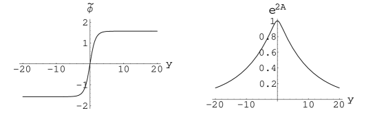
Figure 1: BPS wall solution $\tilde{\phi}(\tilde{y})$ and $A(\tilde{y})$ connecting $\tilde{\phi}=-\pi/2$ to $\tilde{\phi}=\pi/2$.

Let us examine the thin-wall limit [7]. By fixing the energy density $4T^{3}$ and taking a limit $g\rightarrow\infty$, we recover the Randall-Sundrum model [4]. The kinetic energy of the scalar field $|d\phi/dy|^{2}$ reduces to the half of the boundary cosmological constant $\lambda_{\text{boundary}}=4T^{3}=4\Lambda^{3}/g^{2}$, and the remaining half comes from the first term of the scalar potential in Eq.(3) containing derivative of the superpotential. The bulk cosmological constant $\lambda_{\text{bulk}}=-3T^{6}/M_{\rm P}^{2}$ comes from the last term $-3{\rm e}^{|\phi|^{2}/M_{\rm P}^{2}}|P|^{2}/M_{\rm P}^{2}$ of the scalar potential in Eq.(3). These cosmological constants automatically satisfy the relation $\lambda_{\text{boundary}}=4M_{\rm P}\sqrt{-\lambda_{\text{bulk}}/3}$ which was implemented as a fine-tuning in the orbifold model [3]. Our solutions (12) replace the boundary cosmological constant at a fixed point of the orbifold by a smooth physical wall configuration of the scalar field completely. The existence of the thin wall limit suggests that the ${\cal N}=1$ supergravity in four dimensions is consistent even on the orbifold, although we do not know if this point has been demonstrated similarly to the five-dimensional case [5].

We can use the “effective supergravity” to extend our model to arbitrary spacetime dimensions $D$ [9]. Assuming the periodic potential $W(\phi)=(\Lambda^{D-1}/g^{2})\sin(g\phi/\Lambda^{(D-2)/2})$ can be used, we obtain the $D$ dimensional BPS wall solution connecting from $\tilde{\phi}=-\pi/2$ to $\tilde{\phi}=\pi/2$

$$\phi={\Lambda^{D-2\over 2}\over g}\left(2\tan^{-1}e^{\Lambda(y-y_{0})}-\dfrac{\pi}{2}\right),\quad{\rm e}^{2A(y)}=\left[\cosh\Lambda(y-y_{0})\right]^{-{4\over(D-2)g^{2}}\left({\Lambda\over M_{D}}\right)^{D-2}},$$ (13)

with $M_{D}$ as the Planck mass in $D$ dimensions. A BPS wall different from ours has been obtained in a similar model in five-dimensional supergravity [11].

Classification and global properties of Non-BPS Solutions

In order to study possible multi-wall configurations, especially non-BPS configurations, we need to solve the equations of motion which are second order differential equations. It has been shown that these second order equations are equivalent to a set of first order differential equations which resemble the BPS equations provided there is only single scalar field forming walls [8].

Let us assume that initial conditions for complex scalar $\phi(y),d\phi(y)/dy$ and the warp factor $A(y),dA(y)/dy$ are real at some $y$, say $y=-\infty$. The equations of motion for $\phi$ and $A$ in our model then dictate that both $\phi$ and $A$ are real for any $y$. Therefore we can ignore the imaginary part of the complex scalar field as long as we are interested in classical solutions. The bosonic part of the Lagrangian is given by

$$(\sqrt{-g})^{-1}\mathcal{L}=-\dfrac{M_{\rm P}^{2}}{2}R-\!\left({d\phi\over dy}\right)^{2}\!\!-V(\phi),\quad V(\phi)=\dfrac{\Lambda^{4}}{g^{2}}\!\left(\cos^{2}\dfrac{g}{\Lambda}\phi-\dfrac{3\Lambda^{2}}{g^{2}M_{\rm P}^{2}}\sin^{2}\dfrac{g}{\Lambda}\phi\right).$$ (14)

We can now apply the method of Ref.[8] to our model taking $\phi$ as a real scalar field. Given the scalar potential (14), we should find a real function $W(\phi)$ by solving the following first order nonlinear differential equaiton

$$V(\phi)=\left({dW(\phi)\over d\phi}\right)^{2}-{3\over M_{\rm P}^{2}}W^{2}(\phi).$$ (15)

Then $\phi(y)$ and $A(y)$ are obtained by solving the following two first order differential equations

$${d\phi(y)\over dy}=\dfrac{dW(\phi)}{d\phi},\qquad{dA(y)\over dy}=-\dfrac{1}{M_{\rm P}^{2}}W(\phi).$$ (16)

It has been shown that these equations are equivalent to the equations of motion [8].

It is convenient to rewrite these equations in terms of dimensionless variables

$$\tilde{\phi}\equiv\dfrac{g}{\Lambda}\phi,\quad\tilde{W}\equiv{g^{2}\over\Lambda^{3}}W,\quad\tilde{V}\equiv{g^{2}\over\Lambda^{4}}V,\quad\tilde{y}\equiv\Lambda y,\quad\alpha\equiv{\Lambda\over gM_{\rm P}},$$ (17)

$${d\tilde{W}\over d\tilde{\phi}}=\pm\sqrt{\tilde{V}(\tilde{\phi})+3\alpha^{2}\tilde{W}(\tilde{\phi})^{2}},\qquad\tilde{V}(\tilde{\phi})=\cos^{2}\tilde{\phi}-3\alpha^{2}\sin^{2}\tilde{\phi}$$ (18)

$$\dfrac{d\tilde{\phi}}{d\tilde{y}}=\dfrac{d\tilde{W}(\tilde{\phi})}{d\tilde{\phi}},\qquad\dfrac{dA}{d\tilde{y}}=-\alpha^{2}\tilde{W}(\tilde{\phi}).$$ (19)

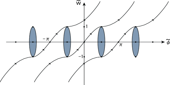
Figure 2: Solution curves of Eq.(18) with $d\tilde{W}/d\tilde{\phi}\geq 0$ in $\tilde{\phi}\tilde{W}$ plane. Forbidden region is shaded.

To obtain a real solution, the right-hand side of Eq.(18) has to be real : $\tilde{V}(\tilde{\phi})+3\alpha^{2}\tilde{W}^{2}\geq 0$. The shaded region in Fig.2 shows the forbidden region in $\tilde{\phi}$ $\tilde{W}$ plane. It is easy to see that the exact (anti-)BPS solutions are those lines whose starting and ending points are both tangent at the top or bottom of these forbidden regions as shown in Fig.2. Any solution is represented by a curve in $\tilde{\phi}$ $\tilde{W}$ plane. Since the first order differential equation (18) determines the solution uniquely once a value of $\tilde{W}$ is specified at some $\tilde{\phi}$ as an initial condition, we observe: 1) No solution curves can intersect. Entire allowed region is covered by the curves once. 2) Curves can end only at the boundary of forbidden region or at infinity.

Taking the positive sign for $d\tilde{W}/d\tilde{\phi}$ in Eq.(18), the asymptotic behavior of solution curves are given by $\tilde{W}\sim\pm\exp(\pm\sqrt{3}\alpha\tilde{\phi})\rightarrow\pm\infty$. As illustrated in Fig.2, there are two different types of curves except the BPS solution curve :

1. Starting at the boundary of forbidden region and ending at $\tilde{\phi},\tilde{W}\rightarrow\infty$.

2. Ending at the boundary of forbidden region and starting at $\tilde{\phi},\tilde{W}\rightarrow-\infty$.

Since the asymptotic behavior $\tilde{\phi},\tilde{W}\rightarrow\pm\infty$ gives singularities [8], [12] at finite $y$ ($y\sim y_{\pm\infty}\mp{\rm e}^{\mp\tilde{\phi}}/(3\alpha^{2})$ as $\tilde{\phi}\rightarrow\pm\infty$), we conclude that BPS wall solution (12) is the only solution which are regular in the entire region of $y$ if we do not allow any external sources for scalar $\phi$ as well as gravity, such as a boundary cosmological constant. If one looks into $\tilde{\phi},\tilde{W}$ plane only, $\tilde{W}=\sin\tilde{\phi}$ may appear a multi-wall winding solution. However, wall solution should be considered as a function of our base space $-\infty<y<\infty$. The solution curve approaches to the top or bottom of the forbidden region only at $y\rightarrow\pm\infty$. Therefore only a segment of $\tilde{W}=\sin\tilde{\phi}$ between the top and the bottom of the forbidden region constitutes a wall solution which is a single wall. The non-existence of multi-wall BPS solutions is perhaps a peculiarity of our model which is in interesting contrast to the monopole or instanton case.

We now wish to find a non-BPS solution by allowing a source due to a boundary cosmological constant $\lambda_{i}\delta(y-y_{i})$ at appropriate points $y=y_{i}$ in the extra dimension into the Lagrangian (14) similarly to the orbifold model [3, 4]. We require that the equation of motion for the scalar field is satisfied without any external sources. Then only the equation of motion for the warp factor is modified to give the boundary condition

$${dA\over dy}(y_{i}+\varepsilon)-{dA\over dy}(y_{i}-\varepsilon)=-\dfrac{1}{2M_{\rm P}^{2}}\lambda_{i}.$$ (20)

The boundary condition combined with Eq.(16) relates the boundary cosmological constant $\lambda_{i}$ at the connection point $\phi=\phi_{i}$ to a discontinuity of $W$ at $\phi=\phi_{i}$

$$\lambda_{i}=2\left(W(\phi_{i}+\epsilon)-W(\phi_{i}-\epsilon)\right).$$ (21)

Equation of motion for $\phi$ without external sources requires both $\tilde{\phi}$ and $d\tilde{\phi}/d\tilde{y}=d\tilde{W}/d\tilde{\phi}$ to be continuous across $y_{i}$.

Let us denote the solution of Eq.(18) specified by the initial condition $(\tilde{\phi}_{0},\tilde{W}_{0})$ as $\tilde{W}_{\pm}(\tilde{\phi};(\tilde{\phi}_{0},\tilde{W}_{0}))$ with the suffix $+(-)$ corresponding to the sign of $d\tilde{W}/d\tilde{\phi}$. Symmetry of Eq.(18) gives

$$\tilde{W}_{\pm}(\tilde{\phi};(\tilde{\phi}_{0},\tilde{W}_{0}))=\tilde{W}_{\pm}(\tilde{\phi}+\pi;(\tilde{\phi}_{0}+\pi,\tilde{W}_{0}))=-\tilde{W}_{\pm}(-\tilde{\phi};(-\tilde{\phi}_{0},-\tilde{W}_{0})),$$ (22)

$$\tilde{W}_{+}(\tilde{\phi};(\tilde{\phi}_{0},\tilde{W}_{0}))=\tilde{W}_{-}(-\tilde{\phi};(-\tilde{\phi}_{0},\tilde{W}_{0}))$$ (23)

As a simple solution to satisfy the requirement of continuity of $\tilde{\phi}$ and $d\tilde{\phi}/d\tilde{y}=d\tilde{W}/d\tilde{\phi}$, we can choose to switch solution curves at $\tilde{\phi}=\pi$ from $\tilde{W}(\tilde{\phi};(0,\tilde{W}_{0}>0))$ to $\tilde{W}(\tilde{\phi};(2\pi,-\tilde{W}_{0}))$ and then at $\tilde{\phi}=2\pi$ to $\tilde{W}(\tilde{\phi};(2\pi,\tilde{W}_{0}))$. As shown in Fig.3 this solution is periodic in $\tilde{\phi}$ with the periodicity $2\pi$, and has a unit winding number and the symmetry $S^{1}/Z_{2}$ which is consistent with the orbifold compactification as in Refs.[3], [4]. We see that we cannot avoid negative cosmological constant (negative energy density). For small $\tilde{W}_{0}$, the solution consists of a BPS wall and an anti-BPS wall at fixed points $\tilde{\phi}=0$ and $\tilde{\phi}=\pi$ of the orbifold supplemented by a small positive cosmological constant at $\tilde{\phi}=0$ and a large negative cosmological constant at $\tilde{\phi}=\pi$. We can similarly construct solutions with arbitrary winding number with or without the orbifold symmetry by connecting solution curves at $\tilde{\phi}=n\pi$ with arbitrary integer $n$. These solutions may be regarded natural in the sense that fixed points occur where the scalar field is localized as walls.

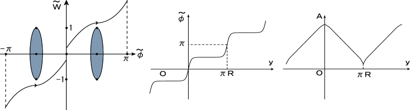
Figure 3: Non-BPS solution with unit winding number. (a) $\tilde{\phi}\tilde{W}$ plane, (b) $\tilde{\phi}(\tilde{y})$, and (c) $A(\tilde{y})$. Discontinuities in $\tilde{W}(\tilde{\phi})$ at $\tilde{\phi}=0,\pm\pi$ correspond to boundary cosmological constants.

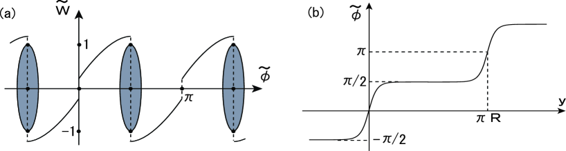
Figure 4: Non-BPS solution with unit winding number with negative boundary cosmological constant at $\tilde{\phi}=\pi/2$. (a) $\tilde{\phi}\tilde{W}$ plane, and (b) $\tilde{\phi}(\tilde{y})$.

If we allow the fixed points of orbifold at the mid point between two walls, we can connect solution curves at $\tilde{\phi}=n\pi+\pi/2$. For instance we can switch solution curves at $\tilde{\phi}=\pi/2$ from $\tilde{W}(\tilde{\phi};(0,\tilde{W}_{0}>0))$ to $\tilde{W}(\tilde{\phi};(\pi,-\tilde{W}_{0}))$ and then at $\tilde{\phi}=\pi$ to $\tilde{W}(\tilde{\phi};(\pi,\tilde{W}_{0}))$. This configuration has a periodicity $\tilde{\phi}=\tilde{\phi}+\pi$ and has a symmetry of $S^{1}/(Z_{2}\times Z_{2})$ orbifold as shown in Fig.4. In the limit of small $\tilde{W}_{0}$, this solution can be regarded as a model essentially replacing the positive cosmological constant by a smooth physical wall configuration of scalar field whereas the negative cosmological constant remains almost the same as in the original model [3], [4]. Actually we can also connect solution curves at arbitrary points in $\tilde{\phi}$ by switching to the curve with the same derivative at the same $\tilde{\phi}$.

Another possibility to connect different solution curves is to switch to curves with opposite sign $d\tilde{W}/d\tilde{\phi}$. This is possible only at the boundary of the forbidden region where $d\tilde{W}/d\tilde{\phi}=0$. If we connect solutions at the boundary of the forbidden region, we can do without putting boundary cosmological constant by switching to the curve starting from the same value of $\tilde{W}$ with the opposite sign for $d\tilde{W}/d\tilde{\phi}$. A typical example with no winding is shown in Fig.5(a). This solution also has the orbifold symmetry $S^{1}/Z_{2}$.

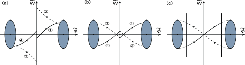
Figure 5: Non-BPS solutions without winding number in $\tilde{\phi}\tilde{W}$ plane. Discontinuities in $\tilde{W}(\tilde{\phi})$ at $\tilde{\phi}=0,\pm\pi$ correspond to boundary cosmological constants. (a) Smooth $\tilde{\phi}$ with two types of boundary cosmological constants at $y=0,\pi R/2$. (b) $\tilde{\phi}$ with only one type of boundary cosmological constant but with a break of scalar field at $y=\pi R/2$. (c) Using a piece of the BPS solution and boundary source for $\phi$.

If we allow boundary cosmological constants at the boundary of the forbidden region, we can connect solutions by switching to the curve starting from the $\tilde{W}$ as well as $d\tilde{W}/d\tilde{\phi}$ of opposite sign at the boundary of forbidden region. We illustrate the simplest of such solution in Fig.5(b). This solution has the symmetry $S^{1}/(Z_{2}\times Z_{2})$ and has no winding number. If we relax our principle and allow the boundary action to contain a source term for the scalar field $\phi$, we have more varieties of solutions. For instance we can even use the BPS solution to construct a solution, simplest of which is illustrated in Fig.5(c). It has the orbifold symmetry $S^{1}/Z_{2}$ but without any cosmological constant at one of the fixed point where the scalar field energy density is localized. This is a model replacing the positive cosmological constant of the original model [3] completely by a smooth thick wall configuration of scalar field at the cost of having a boundary source term for the scalar field in the other fixed point. We can also construct more complicated solutions with or without the orbifold symmetry by combining these various types of boundary cosmological constants.

The precise amount of the cosmological constants and the distance between the walls are determined by Eqs.(18) and (20). We will give a systematic analytic approximation valid for small gravitational coupling below.

A systematic approximation for weak gravity

To establish the limit of no gravity ($\alpha\rightarrow 0$) for the first order differential equations (18) and (19), let us first examine the equation of motion for scalar field $\tilde{\phi}$ without gravity using the scalar potential $\tilde{V}(\tilde{\phi};{\alpha=0})$ in the absence of gravity

$${d\tilde{V}(\tilde{\phi};{\alpha=0})\over d\tilde{\phi}}=2{d^{2}\tilde{\phi}\over d\tilde{y}^{2}}.$$ (24)

By multiplying $d\tilde{\phi}/d\tilde{y}$, we can integrate it once with an integration constant $w_{0}$

$$\tilde{V}(\tilde{\phi};{\alpha=0})=\left({d\tilde{\phi}\over d\tilde{y}}\right)^{2}-3w_{0}^{2}.$$ (25)

This first order differential equation can be identified as the no gravity limit of Eq.(18), if a function $\tilde{W}(\tilde{\phi})$ is defined by $d\tilde{W}/d\tilde{\phi}=d\tilde{\phi}/d\tilde{y}$. Because of Eq.(18), Eq.(19) dictates that the limit of vanishing gravitational coupling is given by

$$\alpha\rightarrow 0,\qquad\alpha\tilde{W}({\tilde{\phi}}=0)\equiv w_{0}\quad{\rm fixed}.$$ (26)

Eqs.(19) and (18) show that $w_{0}=0$ corresponds to the BPS solution.

Since $\tilde{W}_{0}\equiv\tilde{W}({\tilde{\phi}}=0)\sim 1/\alpha\rightarrow\infty$, we define a function $\bar{W}$ more appropriate for an expansion in powers of gravitational coupling $\alpha$

$$\bar{W}(\tilde{\phi})\equiv{\tilde{W}}(\tilde{\phi})-{w_{0}\over\alpha}=\sum_{n=0}^{\infty}\bar{W}^{(n)}(\tilde{\phi}),\quad\tilde{\phi}(\tilde{y})=\sum_{n=0}^{\infty}\tilde{\phi}^{(n)}(\tilde{y}),\quad A(\tilde{y})=\sum_{n=0}^{\infty}A^{(n)}(\tilde{y}).$$ (27)

The first order differential equations appropriate for an expansion in powers of $\alpha$ is

$${d\bar{W}\over d\tilde{\phi}}={d\tilde{\phi}\over d\tilde{y}}=\pm\sqrt{\tilde{V}(\tilde{\phi})+3\left(w_{0}+\alpha{\bar{W}}(\tilde{\phi})\right)^{2}},\quad{dA\over d\tilde{y}}=-\alpha w_{0}-\alpha^{2}\bar{W}(\tilde{\phi}).$$ (28)

It is interesting to note that the first correction is of order $\alpha\equiv\Lambda/(gM_{\rm P})$ rather than the usual $\alpha^{2}$. For our specific model of gravitationally corrected periodic potential, we obtain

$${d\bar{W}^{(0)}\over d\tilde{\phi}}={d\tilde{\phi}^{(0)}\over d\tilde{y}}=\sqrt{\cos^{2}\tilde{\phi}+3w_{0}^{2}},\quad{d\bar{W}^{(1)}\over d\tilde{\phi}}={d\tilde{\phi}^{(1)}\over d\tilde{y}}={3\alpha w_{0}{\bar{W}^{(0)}}\over\sqrt{\cos^{2}\tilde{\phi}+3w_{0}^{2}}},\cdots$$ (29)

$${dA^{(0)}\over d\tilde{y}}=0,\quad{dA^{(1)}\over d\tilde{y}}=-\alpha w_{0},\quad{dA^{(2)}\over d\tilde{y}}=-\alpha^{2}\bar{W}^{(0)}(\tilde{\phi}),\cdots.$$ (30)

The zero-th order equation for $\tilde{\phi}^{(0)}(y)$ in (29) gives precisely our exact non-BPS solution which was obtained in the case of global SUSY [17]

$$\tilde{\phi}^{(0)}(\tilde{y})={\rm am}\left({\tilde{y}-\tilde{y}_{0}\over k},k\right),\qquad k\equiv{1\over\sqrt{1+3w_{0}^{2}}},$$ (31)

$$\bar{W}^{(0)}(\tilde{\phi})={1\over k}\int_{0}^{\tilde{\phi}}d\theta\sqrt{1-k^{2}\sin^{2}\theta}={1\over k}E\left(\tilde{\phi},k\right),$$ (32)

where am is the amplitude function and $E$ is the elliptic integral of the second kind. The warp factor to the zero-th order is given by an irrelevant normalization $A^{(0)}(\tilde{y})=$ constant.

Using Eq.(21), we can now determine to the lowest order in weak gravitational coupling the boundary cosmological constant needed to satisfy the boundary condition (20). For instance, the unit winding solution in Fig.3 requires the boundary cosmological constants $\lambda_{0}$ at $\tilde{\phi}=0$ and $\lambda_{1}$ at $\tilde{\phi}=\pi$

$$\lambda_{0}=4{M_{\rm P}\Lambda^{2}\over g}w_{0},\qquad\lambda_{1}=-4{M_{\rm P}\Lambda^{2}\over g}w_{0}-8{\Lambda^{3}\over g^{2}k}E(k),$$ (33)

where $E(k)$ is the complete elliptic integral of the second kind $E(k)\equiv E(\pi/2,k)$. Similarly other situations can also be expressed in terms of elliptic integrals.

A systematic approximation in powers of gravitational coupling is given by Eq.(29). For instance the first order correction is given by integrating the second of Eq.(29)

$$\tilde{y}-\tilde{y}_{0}=\int_{0}^{\tilde{\phi}^{(1)}}d\theta{\sqrt{1-k^{2}\sin^{2}\theta}\over 3\alpha w_{0}E(\theta,k)},$$ (34)

$$\bar{W}^{(1)}(\tilde{\phi})=\int_{0}^{\tilde{\phi}}d\theta{3\alpha w_{0}E(\theta,k)\over\sqrt{1-k^{2}\sin^{2}\theta}},\qquad A^{(1)}(\tilde{y})=-\alpha w_{0}\tilde{y}.$$ (35)

We can obtain gravitational corrections to any desired order with increasing complexity. We stress that SUSY is not needed for our method to work similarly to Ref.[8]. Therefore it should be useful to obtain solutions for theories with or without gravity irrespective of presence or absence of SUSY.

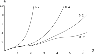
Figure 6: Solution curves of Eq.(18) in $\tilde{\phi}\tilde{W}$ plane with larger gravitational coupling $\alpha=\Lambda/(gM_{\rm P})=0.01,\cdots,1.0$. The curve stays almost the same for $\alpha\leq 0.01$.

Let us also examine the situation with stronger gravitational coupling. The curve stays almost the same for $\alpha\leq 0.01$. We see in Fig.6 that the larger values $\alpha>0.4$ reveal an early emergence of singularities even for relatively smaller values of $\tilde{\phi}$. However, qualitative features remain quite similar for small values of $\tilde{\phi}$. Therefore we expect non-BPS multi-wall configurations are still possible for medium gravitational coupling. It is interesting to note that our BPS solution exists even with strong gravitational couplings at least classically.

Finally we wish to note that the existence of the global SUSY limit (31), (32) implies that we are sure that there is a mass gap for fluctuation modes of the scalar fields. There is a possibility for our wall scalar field $\phi$ to serve as a Goldberger-Wise type stabilizer [20]. We will settle the issue of stability by analyzing the possible new modes associated with the gravity supermultiplet in a subsequent report.

Acknowledgements

One of the authors (N.S.) thanks useful discussion with M. Fukuma, D. Ida, T. Kugo, N. Sasakura, T. Shiromizu, M. Siino, T. Tanaka, Y. Tanii, and A. Van Proeyen. Two of the authors (N.M.,N.S.) are indebted to Y. Sakamura and R. Sugisaka for a collaboration in an early stage. This work is supported in part by Grant-in-Aid for Scientific Research from the Ministry of Education, Science and Culture 13640269. N.M. is supported by the Japan Society for the Promotion of Science for Young Scientists (No.08557).

References

- [1] S. Dimopoulos and H. Georgi, Nucl. Phys. B193 (1981) 150; N. Sakai, Z. f. Phys. C11 (1981) 153; E. Witten, Nucl. Phys. B188 (1981) 513; S. Dimopoulos, S. Raby, and F. Wilczek, Phys. Rev. D24 (1981) 1681.
- [2] N. Arkani-Hamed, S. Dimopoulos and G. Dvali, Phys. Lett. B429 (1998) 263 [hep-ph/9803315]; I. Antoniadis, N. Arkani-Hamed, S. Dimopoulos and G. Dvali, Phys. Lett. B436 (1998) 257 [hep-ph/9804398].
- [3] L. Randall and R. Sundrum, Phys. Rev. Lett. 83 (1999) 3370 [hep-ph/9905221].
- [4] L. Randall and R. Sundrum, Phys. Rev. Lett. 83 (1999) 4690 [hep-th/9906064].
- [5] R. Altendorfer, J. Bagger, and D. Nemeschansky, Phys. Rev. D63 (2001) 125025, [hep-th/0003117]; T. Gherghetta, A. Pomarol, Nucl. Phys. B586 (2000) 141, [hep-ph/0003129]; A. Falkowski, Z. Lalak, and S. Pokorski, Phys. Lett. B491 (2000) 172, [hep-th/0004093]; E.Bergshoeff, R. Kallosh, and A. Van Proeyen, JHEP 0010 (2000) 033, [hep-th/0007044].
- [6] M. Cvetic, S. Griffies and S. Rey, Nucl. Phys. B381 (1992) 301 [hep-th/9201007]; M. Cvetic, and H.H. Soleng, Phys. Rep. B282 (1997) 159 [hep-ph/9804398].
- [7] F.A. Brito, M. Cvetic̆, and S.C. Yoon, Phys. Rev. D64 (2001) 064021, [hep-ph/0105010].
- [8] O. DeWolfe, D.Z. Freedman, S.S. Gubser, and A. Karch, Phys. Rev. D62 (2000) 046008, [hep-th/9909134].
- [9] K. Skenderis, and P.K. Townsend, Phys. Lett. B468 (1999) 46, [hep-th/9909070]; G.W.Gibbons and N.D. Lambert, Phys. Lett. B488 (2000) 90, [hep-th/0003197].
- [10] J. Garriga, and T. Tanaka, Phys. Rev. Lett. 84 (2000) 2778, [hep-th/9911055]; Csaba Csaki, J. Erlich, T. J. Hollowood, and Y. Shirman, Nucl. Phys. B581 (2000) 309, [hep-th/0001033]; S. Ichinose, Phys. Rev. D65 (2002) 084038l, [hep-th/0008245]; K. Behrndt, C. Herrmann, J. Louis, and S. Thomas, JHEP 01 (2001) 011, [hep-th/0008112]; M. Duff, J.T. Lü, and C. Pope, Nucl. Phys. B605 (2001) 234 [hep-th/0009212]; A. Ceresole, G. Dall’Agata, R. Kallosh, and A. Van Preoyen, Phys. Rev. D64 (2001) 104006, [hep-th/0104056]; M. Gremm, Phys. Rev. D62 (2000) 044017, [hep-th/0002040]; M. Cvetic, and N.D. Lambert, Phys. Lett. B540 (2002) 301, [hep-th/0205247].
- [11] K. Behrndt, and G. Dall’Agata, Nucl. Phys. B627 (2002) 357, [hep-th/0112136].
- [12] N. Sasakura, JHEP 0202 (2002) 026 JHEP 0202 (2002) 026, [hep-th/0201130].
- [13] E. Witten and D. Olive, Phys. Lett. B78 (1978) 97.
- [14] G. Dvali and M. Shifman, Phys. Lett. B396 (1997) 64 [hep-th/9612128]; A. Kovner, M. Shifman, and A. Smilga, Phys. Rev. D56 (1997) 7978 [hep-th/9706089]; A. Smilga and A. Veselov, Phys. Rev. Lett. 79 (1997) 4529 [hep-th/9706217]; B. Chibisov and M. Shifman, Phys. Rev. D56 (1997) 7990, [hep-th/9706141]; J. Edelstein, M.L. Trobo, F. Brito and D. Bazeia, Phys. Rev. D57 (1998) 7561 [hep-th/9707016]; V. Kaplunovsky, J. Sonnenschein, and S. Yankielowicz, Nucl. Phys. B552 (1999) 209 [hep-th/9811195]; B. de Carlos and J. M. Moreno, Phys. Rev. Lett. 83 (1999) 2120 [hep-th/9905165]; D. Binosi and T. ter Veldhuis, Phys. Rev. D 63: 085016 (2001), [hep-th/0011113].
- [15] H. Oda, K. Ito, M. Naganuma and N. Sakai, Phys. Lett. B471 (1999) 148 [hep-th/9910095]; K. Ito, M. Naganuma, H. Oda and N. Sakai, Nucl. Phys. B586 (2000) 231 [hep-th/0004188]; Nucl. Phys. Proc. Suppl. 101 (2001) 304 [hep-th/0012182].
- [16] N. Maru, N. Sakai, Y. Sakamura, and R. Sugisaka, Phys. Lett. B496 (2000) 98, [hep-th/0009023].
- [17] N. Maru, N. Sakai, Y. Sakamura, and R. Sugisaka, Nucl. Phys. B616 (2001) 47, [hep-th/0107204]; “SUSY Breaking by Stable non-BPS Walls”, in the Proceedings of the 10th Tohwa international symposium on string theory [hep-th/0109087]; “SUSY Breaking by stable non-BPS configurations”, to appear in the Proceedings of Corfu International Summer Institute, [hep-th/0112244].
- [18] N. Sakai, and R. Sugisaka, “Winding number and non-BPS bound states of walls in nonlinear sigma models” to appear in Phys. Rev. , [hep-th/0203142].
- [19] J. Wess and J. Bagger, “Supersymmetry and Supergravity”, 1991, Princeton University Press.
- [20] W.D. Goldberger and M.B. Wise, Phys. Rev. Lett. 83 (1999) 4922 [hep-th/9907447].