Deconstruction and Gauge Theories in AdS₅
Lisa Randall^a, Yael Shadmi^b and Neal Weiner^c
a Jefferson Physical Laboratory, Harvard University, Cambridge, MA 02138
^b Physics Department, Technion, Haifa 32000, Israel
^c Department of Physics, University of Washington, Seattle, WA, 98195
ABSTRACT

On a slice of AdS₅, despite having a dimensionful coupling, gauge theories can exhibit logarithmic dependence on scale. In this paper, we utilize deconstruction to analyze the scaling behavior of the theory, both above and below the AdS curvature scale, and shed light on position-dependent regularizations of the theory. We comment on applications to geometries other than AdS.

1 Introduction

In recent years, it has become clear that extra dimensions can play an important role in our understanding of the hierarchy problem [1, 2]. In [2], it was noted that the cutoff scale of the standard model could be $O(\rm TeV)$, and yet have weakly coupled gravity if the standard model fields were localized on a brane on the boundary of a slice of AdS₅.

One seeming consequence of having a cutoff at a TeV is that it is impossible to discuss issues of the UV, such as high scale unification. However, this apparent obstacle no longer applies when the gauge sector of the standard model is placed in the bulk of AdS. In particular, in [3] the couplings of fields on the UV brane were studied, and it was demonstrated explicitly that despite the dimensionful bulk gauge coupling, the effective coupling of the zero mode runs logarithmically below the AdS curvature scale. In [4, 5], a position-dependent regulator motivated by holography was used to show that the predictions of perturbative high-scale unification were possible, even in theories where standard model fields experience a strong-coupling cutoff at the TeV scale. More recently, [6, 7, 8, 9, 10, 11] have studied the behavior of gauge fields in AdS. All of these works agree that, at some level, gauge running in AdS is logarithmic, rather than power law, below the compactification scale. However, there nonetheless remains some confusion as to what constitutes a sensible regulator, and in what sense one can talk about a zero mode definitively above the IR brane scale.

Over the past year, “deconstruction” [12, 13] has a appeared as a new tool for model building and understanding the properties of higher-dimensional gauge theories. By viewing the higher-dimensional theory as a product of four-dimensional theories, one can easily study the properties of the theory at intermediate energies. In this paper, we will employ deconstruction to give us an understanding of the properties of AdS gauge theories at energies above the scale of the IR brane. We, too, will recover log running above a TeV, but we will also see how position dependent regulators naturally arise in the deconstructed framework. We also will recover cutoff sensitive “power-law running” effects above the curvature scale, which will appear as threshold effects associated with the cutoff of the theory. We will also see in what sense we can discuss a renormalized zero mode above the IR brane scale. Lastly, the results we achieve can be straightforwardly applied to different geometries.

2 Gauge Theories in AdS

Five dimensional gauge field theories are defined as cutoff theories. Because the gauge coupling is dimensionful, there is an associated ultra-violet strong coupling scale. However, AdS gauge theories present a number of subtleties not found in flat extra dimensions.

In flat extra dimensions, we see the first Kaluza-Klein mode at a scale $1/R$. At a scattering energy $E\simeq n/R$, one exchanges $n$ KK modes, giving a strong coupling scale $\Lambda\sim 4\pi/Rg_{4}^{2}\sim 4\pi^{2}/g_{5}^{2}$. Note that we could live on a brane at any point in the space and this formula would remain essentially unchanged.

In AdS, the situation is quite different. If we consider the RS1 space with UV and IR cutoff branes, the mass of the first KK mode is set by the IR scale as is the spacing between KK modes. Thus, a scattering at a high scale $\Lambda\gg M_{IR}$ would naively be strongly coupled. The essential difference in AdS is that this is a position dependent question. In the language of KK modes, this is because the light KK modes are strongly coupled to the IR brane, but very weakly coupled to the UV brane.

This result is not surprising because it arises from the basic symmetries of AdS. Let us consider a $U(1)$ gauge theory in AdS. We can write the metric as

$$ds^{2}=e^{-2\sigma(y)}dx^{4}-dy^{2}\ .$$ (1)

For now and unless otherwise noted, we take $\sigma(y)=ky$. With this metric, the gauge boson action is

$$S=-{1\over 4}\,\int d^{4}xdy{1\over g_{5}^{2}}\,\left[G_{\mu\nu}^{2}-2e^{-2\sigma}G_{\mu 5}^{2}\right]\ ,$$ (2)

where all 4d contractions are with $\eta_{\mu\nu}$. Note that this action is invariant under the transformation

$$y\rightarrow y+\delta,$$ (3)

$$x\rightarrow e^{k\delta}x,$$ (4)

$$\partial_{\mu}\rightarrow e^{-k\delta}\partial_{\mu},$$ (5)

$$A_{\mu}\rightarrow e^{-k\delta}A_{\mu}.$$ (6)

The transformation of the gauge field is necessary to insure that gauge covariant derivatives of charged fields are also covariant under the rescaling.

This symmetry tells us that a process with four-momentum $p_{\mu}$ at a point $y=y_{0}$ relates to an equivalent process with four-momentum $e^{-k\delta}p_{\mu}$ at a point $y^{\prime}=y_{0}+\delta$. Or (not surprisingly) the local (in $y$) strong coupling scale scales with the warp factor.

In going to the quantum theory, we have to be careful in how we define our couplings. In four-dimensional QED, for instance, we define the coupling $e$ at a scale $\mu_{0}$, with the same $e$ and the same $\mu_{0}$ everywhere. This is a requirement for preserving the Poincaré invariance of the theory. In AdS we do not have five-dimensional Poincaré invariance so we must be careful to define our theory to preserve the symmetries.

One way we cannot define the theory is to specify all couplings at the scale of the UV brane. This is because over most of the space the gauge theory becomes strongly coupled below this scale, and hence this is not even a region in which the perturbative field theory is defined.

Likewise, we could specify the couplings at the scale of the IR brane, but this is troubling as we take the IR brane to infinity, and, moreover, it would spoil the symmetries of the theory. Hence, the most natural definition, the one that maintains the symmetry of the space, is to assume that the couplings are specified at a scale which scales with the warp factor in $y$. This will be essential in writing down the deconstructed quantum theory.

3 The classical deconstructed theory

Let us begin by reviewing the standard process of deconstruction. Our goal will be to write a five-dimensional $SU(n)$ as a four-dimensional, $SU(n)^{N}$ gauge theory with bifundamental fields, $Q_{i}$ (see table 1) with

$$\langle Q_{i}\rangle=v_{i}\,{\rm diag}(1,1,\cdots,1).$$ (7)

The lattice will more accurately reproduce intermediate scale physics with increasing $N$, the number of lattice sites. Most importantly, the theory is cut off at a local scale $\Lambda_{j}\sim v_{j}$, so that we can regulate our theory in a gauge-invariant fashion.

From the outset, deconstruction of an AdS gauge theory is quite different from the deconstruction of one in flat space. In flat space, if a fermion is localized at any point in the additional dimension(s), it will couple with comparable strength to each of the KK modes. Consequently, accurately reproducing the intermediate energy features in the deconstructed theory requires matching states and energies.

The AdS case is quite different. Above the local AdS curvature scale, the gauge theory quickly becomes strongly coupled. However, those KK modes are very weakly coupled to the UV brane, so in a deconstructed theory, these modes will be automatically grouped, depending on the coarseness of the latticization, into single modes whose effects will replace multiple modes in the extra dimensional theory. While this seems peculiar, it is precisely because those modes are so weakly coupled that this remains a true description of the features of the higher dimensional theory.

We begin by discretizing the 5th dimension in (2). We have

$$S=-{1\over 4}\,\int d^{4}x\,\left[\sum_{j}{a_{j}\over g_{5j}^{2}}{G_{\mu\nu}^{(j)}}^{2}-2\sum_{j}{a_{j}e^{-2\sigma_{j}}\over g_{5j}^{2}}\,{G_{\mu 5}^{(j)}}^{2}\right]\ ,$$ (8)

where $j$ denotes the lattice site, $a_{j}$ is the lattice spacing near site $j$, $a_{j}=y_{j+1}-y_{j}$ and $j=1\ldots N$, and

$$G_{\mu 5}^{(j)}=\partial_{\mu}A_{5}^{(j)}-{1\over a_{j}}\,(A_{\mu}^{(j+1)}-A_{\mu}^{(j)})\ .$$ (9)

To write down a lattice action we can replace $A_{5}$ by the link fields

$$U=e^{i\int_{y_{j}}^{y_{j+1}}dyA_{5}(x,y)}\ ,$$ (10)

so that for small lattice spacing,

$$D_{\mu}U\sim i(a_{j}\partial_{\mu}A_{5}^{j}-A_{\mu}^{j}+A_{\mu}^{j+1})\ .$$ (11)

$$\begin{array}[]{c|ccccc}&SU(n)_{1}&SU(n)_{2}&SU(n)_{3}&\cdots&SU(n)_{N}\\ \hline\cr Q_{1}&\raisebox{-0.5pt}{\hbox{\rule{0.4pt}{6.5pt}\hskip-0.4pt\rule{6.5pt}{0.4pt}\hskip-6.5pt\rule[6.5pt]{6.5pt}{0.4pt}}\rule[6.5pt]{0.4pt}{0.4pt}\hskip-0.4pt\rule{0.4pt}{6.5pt}}&\overline{\raisebox{-0.5pt}{\hbox{\rule{0.4pt}{6.5pt}\hskip-0.4pt\rule{6.5pt}{0.4pt}\hskip-6.5pt\rule[6.5pt]{6.5pt}{0.4pt}}\rule[6.5pt]{0.4pt}{0.4pt}\hskip-0.4pt\rule{0.4pt}{6.5pt}}}&1&\cdots&1\\ Q_{2}&1&\raisebox{-0.5pt}{\hbox{\rule{0.4pt}{6.5pt}\hskip-0.4pt\rule{6.5pt}{0.4pt}\hskip-6.5pt\rule[6.5pt]{6.5pt}{0.4pt}}\rule[6.5pt]{0.4pt}{0.4pt}\hskip-0.4pt\rule{0.4pt}{6.5pt}}&\overline{\raisebox{-0.5pt}{\hbox{\rule{0.4pt}{6.5pt}\hskip-0.4pt\rule{6.5pt}{0.4pt}\hskip-6.5pt\rule[6.5pt]{6.5pt}{0.4pt}}\rule[6.5pt]{0.4pt}{0.4pt}\hskip-0.4pt\rule{0.4pt}{6.5pt}}}&\cdots&1\\ &\vdots&\vdots&\vdots&\ddots&\vdots\\ Q_{N-1}&1&1&1&\cdots&\overline{\raisebox{-0.5pt}{\hbox{\rule{0.4pt}{6.5pt}\hskip-0.4pt\rule{6.5pt}{0.4pt}\hskip-6.5pt\rule[6.5pt]{6.5pt}{0.4pt}}\rule[6.5pt]{0.4pt}{0.4pt}\hskip-0.4pt\rule{0.4pt}{6.5pt}}}\\ \end{array}$$

Table 1: Field content for a deconstructed $SU(n)$ theory.

Let us now consider the action of the deconstructed theory,

$$S=\int d^{4}x\left[-{1\over 4}\sum_{j}{1\over g_{j}^{2}}{F_{\mu\nu}^{(j)}}^{2}+\sum_{j}{1\over g_{j}^{2}}\,D_{\mu}Q_{j}^{\dagger}D^{\mu}Q_{j}\right]\ .$$ (12)

The peculiar normalization for the matter fields is convenient since they will ultimately supply the 5th component of the gauge fields. In the supersymmetric version of the theory, which we will later consider, this normalization allows for a holomorphic definition of the length of the 5th dimension, since the gauge coupling does not appear in the relation between this length and the VEVs.

Assuming all $Q$’s get VEVs we have $N-1$ $\sigma$-models, coupled by the gauge interaction. Writing $Q_{j}=v_{j}{\tilde{U}}_{j}$, we choose the parameters of the deconstructed theory, $v_{j}$ ang $g_{j}$, so that the action (12) agrees with the 5d lattice action (8):

$${1\over g_{j}^{2}} = {a_{j}\over g^{2}_{5j}},$$ (13)

$${v_{j}^{2}\over g_{j}^{2}} = {e^{-2\sigma_{j}}\over a_{j}g^{2}_{5j}}\ ,$$

so that,

$$v_{j}^{2}={e^{-2\sigma_{j}}\over a_{j}^{2}}\ .$$ (14)

Here we see the effect of the AdS geometry. While a theory with five-dimensional Lorentz invariance naturally has a deconstructed description with all VEVs, $v_{j}$, equal, here the $v_{j}$’s scale with the warp factor. We also note that, with conventional normalization for the bifundamentals, the gauge coupling would appear in (14).

We thus have a “dictionary” between the 5d parameters — the gauge coupling, $g_{5j}$, and the lattice spacing $a_{j}$ — and the parameters of the deconstructed theory, $v_{j}$ and $g_{j}$.

One can consider different variations of this basic theory. For example, in order to study bulk matter, we can add matter fields for every $SU(n)$ factor. In the supersymmetric version of the theory (with ${\cal N}=1$ supersymmetry), one needs to add matter in order to cancel anomalies on the two ends of the chain. A simple possibility is to add fundamentals and antifundamentals as shown in table 2.

$$\begin{array}[]{c|ccccc}&SU(n)_{1}&SU(n)_{2}&SU(n)_{3}&\cdots&SU(n)_{N}\\ \hline\cr{\bar{q}}_{i=1\ldots n}&\overline{\raisebox{-0.5pt}{\hbox{\rule{0.4pt}{6.5pt}\hskip-0.4pt\rule{6.5pt}{0.4pt}\hskip-6.5pt\rule[6.5pt]{6.5pt}{0.4pt}}\rule[6.5pt]{0.4pt}{0.4pt}\hskip-0.4pt\rule{0.4pt}{6.5pt}}}&1&1&\cdots&1\\ q_{a=1\ldots n}&1&1&1&\cdots&\raisebox{-0.5pt}{\hbox{\rule{0.4pt}{6.5pt}\hskip-0.4pt\rule{6.5pt}{0.4pt}\hskip-6.5pt\rule[6.5pt]{6.5pt}{0.4pt}}\rule[6.5pt]{0.4pt}{0.4pt}\hskip-0.4pt\rule{0.4pt}{6.5pt}}\\ \end{array}$$

Table 2: Adding vectorlike fields at the end sites cancels anomalies in the supersymmetric theory.

These fields can get mass through non-renormalizable operators [16], or through extra vectorlike matter [17]. However, they do not affect our basic analysis and results.

3.1 Couplings at intermediate energies in the deconstructed theory

To get a sense of the behavior of the deconstructed theory, let us begin by considering the exchange of a bulk gauge field coupling to a field on the UV brane at energies $R^{-1}\gg q\gg\rm TeV$. Being confined to the UV brane is equivalent to being charged under the gauge group $G_{1}$ in the deconstructed theory.

At very low energies, the entire theory is Higgsed to the diagonal. Then the two-point function in the Feynman-t’Hooft gauge for exchange of a bulk gauge boson between two fields on the UV brane is given simply by

$$G_{q}(0)\eta^{\mu\nu}\simeq-i\frac{g^{2}}{N}\frac{\eta^{\mu\nu}}{q^{2}}.$$ (15)

At a higher energy $q\gg\rm TeV$, we have resolved the independent gauge groups Higgsed down below a scale q, and instead, the dominant contribution comes from the exchange of the diagonal gauge field of the groups which have been Higgsed down at energies above $q$. This behavior is shown in figure 1.

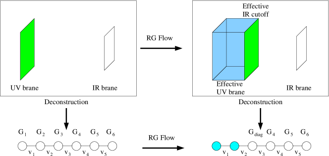
Figure 1: Connection between RG flow in the continuum and deconstructed theory. A high energy theory has the massive modes (localized near the UV brane) integrated out to leave a different theory with a different UV brane with large kinetic terms for the bulk gauge field. For momentum $q$ processes occuring on the UV brane, the dominant contribution to exchange comes from the diagonal mode of the shaded region, yielding an effective IR cutoff in the continuum theory.

The effective number of groups contained in the diagonal at a scale $q$ can be written approximately as

$$aN_{eff}\simeq R\log(q/\Lambda).$$ (16)

Now we can approximate the exchange of the gauge field by the diagonal mode, yielding

$$G_{q}(0)\eta^{\mu\nu}\approx-i\frac{g^{2}}{N_{eff}}\frac{\eta^{\mu\nu}}{q^{2}}\approx-i\frac{g_{5}^{2}k}{\log(q/\Lambda)q^{2}}\,\eta^{\mu\nu},$$ (17)

where we have used the relation $g_{5}^{2}=g^{2}a$.

It is notable that the dominant classical logarithmic scaling for the AdS gauge field two-point function falls out automatically from the deconstructed theory, without invoking any further assumptions about the holographic nature of the theory. This is an excellent indication that the deconstructed theory is effectively reproducing the physics of the five-dimensional theory.

3.2 Couplings at high energies in the deconstructed theory

At high energies, our coarse latticization is insufficient. If we want to understand physics near the strong coupling scale of the theory, we should latticize such that each $\alpha_{j}=g_{j}^{2}/4\pi\approx 4\pi$. However in this case the separation of VEVs is small, that is, the $\sigma_{j}$’s are close together, and one would need to diagonalize the gauge boson mass matrix, and determine couplings to each mode. However, since the VEVs are close together, the result is obvious: groups Higgsed down significantly below the UV cutoff are irrelevant (classically), and groups Higgsed at a scale roughly an factor of a few down from the cutoff act nearly as a flat extra dimension with radius $R_{eff}\sim 1/k$, as expected.

4 Gauge coupling running in deconstructed RS

Before we can talk about running of the gauge coupling, we must define what we mean, precisely. We cannot speak perturbatively about fields on the TeV brane scattering at energies well above a TeV. In what sense can we discuss running?

The answer is actually quite straightforward. At low energies, fields on the TeV brane scatter through the zero mode of the five-dimensional theory. Likewise, fields on the UV brane scatter at low energies with equal couplings (as required by the remaining four dimensional gauge invariance). Thus, we can relate measured gauge couplings on the TeV brane to those that would exist for fields on the UV brane. We can then ask questions about two-point functions at higher energies on the UV brane.

The deconstructed theory is characterized by two sets of parameters: the dimensionless couplings $g_{j}$, and the dimensionful VEVs $v_{j}$. As discussed above, in order to mimic the continuum theory, we choose

$$v_{j}=ve^{-jw},$$ (18)

with $w=ka$. In addition, the individual couplings are defined at the scale of the corresponding VEVs, that is,

$$g_{j}=g_{j}(v_{j})=g\ ,$$ (19)

or, in terms of the strong coupling scales of the individual groups,

$$\Lambda_{j}^{b}=v_{j}^{b}\,e^{-{8\pi^{2}\over g^{2}}},$$ (20)

where $b$ is the one-loop beta function coefficient, which is the same for all groups. Examining the relations (13), we see that this indeed corresponds to taking $g_{5j}=const$ and $a_{j}=a$.

It is instructive to start by considering a coarse lattice, with the lattice spacing larger than the AdS curvature: $a\gg k^{-1}$. Then we have

$$v_{1}\gg v_{2}\gg\cdots\gg v_{N-1}\ .$$ (21)

This simplifies the analysis considerably: we can study the running by turning on the VEVs one at a time. It is amusing that the RS case turns out to be simpler to analyze than the flat case, where all VEVs are equal and therefore have to be considered together.

Let us now derive the coupling of the low energy theory. At the scale $v_{1}$, $SU(n)_{1}\times SU(n)_{2}$ is broken to the diagonal subgroup, which we label $SU(n)_{2D}$ (with the diagonal group of $j$ groups labeled $SU(n)_{jD}$), with gauge coupling,

$${1\over g_{2D}^{2}(v_{1})}={1\over g_{1}^{2}(v_{1})}+{1\over g_{2}^{2}(v_{1})}\ .$$ (22)

We can now run down to the scale $v_{2}$, where,

$${1\over g_{2D}^{2}(v_{2})}={1\over g_{1}^{2}(v_{1})}+{1\over g_{2}^{2}(v_{1})}+{b\over 8\pi^{2}}\,\ln{v_{2}\over v_{1}}\ ,$$ (23)

where we used the fact that the diagonal subgroups have the same beta function coefficients as the original group factors.

Repeating this $j$ times we find,

$${1\over g_{jD}^{2}(v_{j})}={1\over g_{1}^{2}(v_{1})}+\cdots+{1\over g_{j}^{2}(v_{j})}+{b\over 8\pi^{2}}\,\ln{v_{j}\over v_{1}}\ .$$ (24)

Using the fact that $k=-w^{-1}\ln{v_{j}/v}$, and $g_{5}^{2}=ag^{2}$, this can be written as

$${1\over g_{D}^{2}(v_{j})}=-{1\over kg_{5}^{2}}\,\ln{v_{j}\over v}+{b\over 8\pi^{2}}\ln{\mu\over v}-{b\over 8\pi^{2}}ka$$ (25)

Indeed, the low energy coupling depends logarithmically on the scale. In fact, we see that the low energy coupling contains two pieces with logarithmic energy dependence. The first term on the RHS of eqn. (25) is a classical piece, which reproduces the fact that the 4d and 5d couplings are related by the “radius”. In the deconstructed theory, it is obtained by summing over KK modes at tree level. The second piece is a loop effect. It is obtained from running the coupling between adjacent KK modes.

Let us now consider the supersymmetric theory. In the presence of ${\cal N}=1$ supersymmetry, holomorphy and symmetries dictate the dependence of the diagonal $SU(n)$ strong coupling scale, $\Lambda_{D}$, on $\Lambda_{j}$, $v_{j}$, at any stage of the Higgsing. In particular, at low energies,

$$\Lambda_{D}^{b}\sim{\Lambda_{1}^{b}\ldots\Lambda_{N}^{b}\over N^{b}v_{1}^{b}\ldots v_{N-1}^{b}}.$$ (26)

The factor of $N^{b}$ is not dictated by symmetries, but can be found from explicit computation [18].

The relation (26) allows us to obtain the low energy coupling for any profile of the VEVs. In particular, for the RS geometry, with (18), (20), we have at low energy

$${1\over g_{L}^{2}(\mu)}={N\over g^{2}}+{b\over 8\pi^{2}}\ln{\mu\over v/N}.$$ (27)

Running from a scale below $k$, deconstruction yields ordinary logarithmic running with a beta function set by the four-dimensional gauge theory. In terms of the parameters of the theory, this gives us

$$\simeq-{1\over kg_{5}^{2}}\,\ln{v_{N-1}\over v}+{b\over 8\pi^{2}}\ln{\mu\over v/N}={R\over g_{5}^{2}}+{b\over 8\pi^{2}}\ln{\mu\over v/N}.$$ (28)

This indeed reproduces the expression we found for the non-supersymmetric theory. Again, we see the logarithmic dependence on the energy scale in both the tree-level and one-loop pieces.

4.1 Fine Latticizations and Power Law Running

So far we have seen that a coarse latticization of AdS can generate the log running behavior which is characteristic of these gauge theories. But what about energies above $k$? At these energies the space is approximately flat and there is a possible power law contribution between $k$ and $\Lambda$.

This arises from a subtlety which we have to this point ignored. We have defined our couplings $g_{j}$ at the scale $v_{j}$. This was reasonable because the scales varied with energy, preserving the symmetries of the theory. Also, $v_{j}$ is approximately the local cutoff, so if we believe the unfication is only manifest in a microscopic theory (e.g. string theory), this is the approximately the cutoff scale (which is ambiguous).

These ambiguities make little difference when the coupling scales logarithmically with the cutoff, but is very important in the power law piece. To extract the behavior most straightforwardly, we will consider the supersymmetric theory, but the presence of the power law piece will not depend on the supersymmetric matter content. Consider again (26). If we state that the couplings unify at a scale $M_{j}\sim v_{j}$ we have

$$\Lambda_{D}^{b} \sim {\Lambda_{1}^{b}\ldots\Lambda_{N}^{b}\over N^{b}v_{1}^{b}\ldots v_{N-1}^{b}},$$ (29)

$$\mu e^{8\pi^{2}/g_{D}^{2}(\mu)} \sim {\Lambda_{1}^{b}\ldots\Lambda_{N}^{b}\over N^{b}M_{1}^{b}\ldots M_{N-1}^{b}}\times\frac{M_{1}^{b}\ldots M_{N-1}^{b}}{v_{1}^{b}\ldots v_{N-1}^{b}},$$ (30)

$$\sim v^{b}e^{8\pi^{2}N/g^{2}}e^{\gamma Nb},$$ (31)

where $\gamma=\log(M_{j}/v_{j}N^{1/N})$ is independent of $j$.

Restating this in terms of gauge couplings, we have

$$\frac{1}{g_{D}^{2}(\mu)}=\frac{N}{g^{2}}+\frac{b}{8\pi^{2}}\log(v/\mu)+\frac{Nb\gamma}{8\pi^{2}}.$$ (32)

Note that we have made no assumptions about the background geometry to derive this result - it can be applied to any space. In AdS we recognize the first term as the usual $R/g_{5}^{2}=\log(v/v_{N-1})/kg_{5}^{2}$ piece, and the second we recognize as the log running piece. The final piece is the power law running piece. Using the relation

$$N=\frac{R}{a}=\frac{v\log(v/v_{N-1})}{k},$$ (33)

we can rewrite (32) as

$$\frac{1}{g_{D}^{2}(\mu)}=\frac{N}{g^{2}}+\frac{b}{8\pi^{2}}\log(v/\mu)+\frac{vb\gamma}{8\pi^{2}k}\log(v/v_{N-1}).$$ (34)

Taking $v\sim\Lambda$, we see the linear cutoff dependence (“power law running”) explicitly. This term is worthy of two observations. The first is that it seems that merely by restating the each $g_{j}$ at $v_{j}$ we could remove the power dependence. It is true that a suitable redefinition of $g_{5}^{2}$ can absorb this piece entirely. However, since we are ultimately considering the possibility of unification, we cannot do this as the separate redefinitions of couplings for $3-2-1$ would not be $SU(5)$ symmetric. Hence, in considering differences of couplings, this is a real effect.

The second observation is that there is essentially a free parameter in the theory, $\gamma$. This is not surprising because the theory has a linear divergence, implying cutoff sensitivity. We have employed a particular cutoff which has an ambiguity: namely the unification scale relative to the cutoff scale. This uncertainty is reasonable from an effective field theory perspective as it merely parameterizes our ignorance of the physics which generates the low energy field theory. In terms of the continuum theory, the upshot is that while there is true power law dependence on the cutoff, the coefficient of this term is unknown. That being said, it should also be noted that the relative strengths of these cutoff terms are still proportional to the relevant $\beta$ functions.

Lastly, we note that here the power law piece can be subdominant to the log running piece. We would expect additional threshold effects comparable to the power law piece in any complete model, which could easily spoil quantitative unification. In AdS, because the log piece can dominate for unification scales below the strong coupling cutoff of the theory, the GUT-violating threshold effects are under control and one can still speak reliably about unification.

5 Position Dependent Regularizations from Deconstruction

In [5], a position dependent cutoff was used to study the evolution of gauge couplings in a warped background. The regularization employed was an energy dependent IR brane, which was motivated by holography and the presence of strong coupling away from the UV brane at intermediate energy. Here, this regularization arises naturally from the deconstructed theory, without appealing to holography.

Let us begin by running the theory down from high energies. In the deconstructed theory, we gradually Higgs down more and more groups such that the highest energy group becomes more weakly coupled. At each level we integrate out the classical and quantum fluctuations of only the left-most groups in the quiver diagram. If we treat deconstruction as an invertible map, the resulting position space regularization is illustrated in figure 1.

In the deconstructed picture the appropriate regularization is obvious. One merely integrates out the heavy modes, which exist near the UV brane, and replaces the theory with a different one, with a new UV brane positioned nearer to the IR, but now with large boundary kinetic terms corresponding to the modes integrated out.

Of course, this relates the fundamental Lagrangian with a lower energy effective theory. We also want to ask questions about the relationship between low-energy and high-energy scatterings on the UV brane. Here, our interpretation of the above diagram is somewhat different. At any given momentum $q$, we are cut off from the sites Higgsed at scales less than $q$. As a consequence, we should calculate loops only with the modes from the sites at energies above $q$. In particular, as we have already argued, the dominant contribution to the two-point function comes from the diagonal mode of the sites at energies above $q$.

Mapping the deconstructed theory back to the continuum, we see that we have introduced an IR cutoff on the theory, and the diagonal mode of the sites above $q$ maps to the zero mode of the theory with this IR brane in place. Thus, while one cannot safely talk about couplings of the zero mode of the complete theory at high energies (because of strong couplings in the IR) one can reasonably talk about the zero mode of the theory with a different IR cutoff. It is notable that the deconstructed picture forces this regularization on us, and we need not appeal to holographic intuition.

Lastly, we note that these regularizations should also appear automatically in other, non-trivial geometries. In situations without an obvious regularization, the deconstructed approach, with VEVs following the warp factor, should give the appropriate position dependent regularization.

6 Conclusions

Extra dimensional theories with TeV-scale cutoffs invite careful analysis of questions regarding the ultra-violet. In the AdS slice of RS1, the introduction of gauge fields into the bulk offers the possibility of discussing short distance physics, such as coupling constant unification.

The application of deconstruction to this question obviates many of the questions raised in continuum theory analyses. Position dependent regulators appear automatically in the deconstructed framework, motivating their use in studying continuum theories.

Note added: While this work was being prepared, [19] appeared which addresses similar issues. The authors would also like to acknowledge unpublished work on this subject by N. Arkani-Hamed and A. Cohen.

Acknowledgements The authors thanks Kaustubh Agashe, Antonio Delgado, Walter Goldberger, Witek Skiba, Veronica Sanz, Erich Popptiz and especially Yuri Shirman and Nima Arkani-Hamed for useful discussions. Y.S. and N.W. would like to thank the visitor program at Harvard University where this work was initiated, and the Aspen Center for Physics where much of this work was completed.

References

- [1] N. Arkani-Hamed, S. Dimopoulos and G. R. Dvali, “The hierarchy problem and new dimensions at a millimeter,” Phys. Lett. B 429, 263 (1998) [arXiv:hep-ph/9803315].
- [2] L. Randall and R. Sundrum, “A large mass hierarchy from a small extra dimension,” Phys. Rev. Lett. 83, 3370 (1999) [arXiv:hep-ph/9905221].
- [3] A. Pomarol, “Grand unified theories without the desert,” Phys. Rev. Lett. 85, 4004 (2000) [arXiv:hep-ph/0005293].
- [4] L. Randall and M. D. Schwartz, “Unification and the hierarchy from AdS5,” Phys. Rev. Lett. 88, 081801 (2002) [arXiv:hep-th/0108115].
- [5] L. Randall and M. D. Schwartz, “Quantum field theory and unification in AdS5,” JHEP 0111, 003 (2001) [arXiv:hep-th/0108114].
- [6] W. D. Goldberger and I. Z. Rothstein, “High energy field theory in truncated AdS backgrounds,” arXiv:hep-th/0204160.
- [7] K. Agashe, A. Delgado and R. Sundrum, “Gauge coupling renormalization in RS1,” arXiv:hep-ph/0206099.
- [8] K. w. Choi, H. D. Kim and I. W. Kim, “Radius dependent gauge unification in AdS(5),” arXiv:hep-ph/0207013.
- [9] R. Contino, P. Creminelli and E. Trincherini, “Holographic evolution of gauge couplings,” arXiv:hep-th/0208002.
- [10] W. D. Goldberger and I. Z. Rothstein, “Effective Field Theory and Unification in AdS Backgrounds,” arXiv:hep-th/0208060.
- [11] K. w. Choi and I. W. Kim, “One loop gauge couplings in AdS5,” arXiv:hep-th/0208071.
- [12] N. Arkani-Hamed, A. G. Cohen and H. Georgi, “(De)constructing dimensions,” Phys. Rev. Lett. 86, 4757 (2001) [arXiv:hep-th/0104005].
- [13] C.T. Hill, S. Pokorski and J. Wang, “Gauge invariant effective lagrangians for kaluza-klein modes”, Phys. Rev. D64, 105005 (2001) [arXiv:hep-th/0104035].
- [14] H. C. Cheng, C. T. Hill and J. Wang, “Dynamical electroweak breaking and latticized extra dimensions,” Phys. Rev. D 64, 095003 (2001) [arXiv:hep-ph/0105323].
- [15] H. Abe, T. Kobayashi, N. Maru and K. Yoshioka, “Field localization in warped gauge theories,” arXiv:hep-ph/0205344.
- [16] C. Csaki, J. Erlich, C. Grojean and G. D. Kribs, “4D constructions of supersymmetric extra dimensions and gaugino mediation,” Phys. Rev. D 65, 015003 (2002) [arXiv:hep-ph/0106044].
- [17] W. Skiba and D. Smith, “Localized fermions and anomaly inflow via deconstruction,” Phys. Rev. D 65, 095002 (2002) [arXiv:hep-ph/0201056].
- [18] C. Csaki, J. Erlich, V. V. Khoze, E. Poppitz, Y. Shadmi and Y. Shirman, “Exact results in 5D from instantons and deconstruction,” Phys. Rev. D 65, 085033 (2002) [arXiv:hep-th/0110188].
- [19] A. Falkowski and H. D. Kim, arXiv:hep-ph/0208058.