Dirac Spectra and Real QCD at Nonzero Chemical Potential

Abstract

We show that QCD Dirac spectra well below $\Lambda_{\rm QCD}$, both at zero and at nonzero chemical potential, can be obtained from a chiral Lagrangian. At nonzero chemical potential Goldstone bosons with nonzero baryon number condense beyond a critical value. Such superfluid phase transition is likely to occur in any system with a chemical potential with the quantum numbers of the Goldstone bosons. We discuss the phase diagram for one such system, QCD with two colors, and show the existence of a tricritical point in an effective potential approach.

1 Introduction

For strongly interacting quantum field theories such as QCD a complete nonperturbative analysis from first principles is only possible by means of large scale Monte Carlo simulations. Therefore, partial analytical results in some parameter domain of the theory are extremely valuable, not only to provide additional insight in the numerical calculations, but also as an independent check of their reliability. This has been our main motivation for analyzing such domains. The principle idea we have been pursuing is based on chiral perturbation theory [ [1, 2]]: because of confinement and the spontaneous breaking of chiral symmetry, the low-energy chiral limit of QCD is a theory of weakly interacting Goldstone bosons which are described by a chiral Lagrangian that is completely determined by the symmetries of QCD. This idea can be applied to the QCD Dirac spectrum which can be extracted from the valence quark mass dependence of the chiral condensate. The valence quark mass is not a physical parameter of the QCD partition function and can be chosen in a domain where the valence quark mass dependence of the QCD partition function can be described to an arbitrary accuracy by a corresponding chiral Lagrangian. If the Compton wavelength of Goldstone bosons containing only valence quark masses is much larger than the size of the box the low-energy effective theory simplifies even much further [ [3]]. Then only the zero momentum component of the Goldstone fields has to be taken into account so that the valence quark mass dependence of the QCD partition function is given by a unitary matrix integral. This idea was first applied to the QCD partition function [ [4]] with quark masses of order $m\sim 1/V\langle\bar{\psi}\psi\rangle$ (with $\langle\bar{\psi}\psi\rangle$ the chiral condensate and $V$ the volume of space-time). However, we emphasize that for physical values of the quark masses and volumes, a part of the Dirac spectrum, as probed by the valence quark mass, is always in this mesoscopic domain of QCD. More precisely, using the Gell-Mann-Oakes-Renner relation (with $F$ the pion decay constant), in the domain

$$\frac{m_{v}\langle\bar{\psi}\psi\rangle}{F^{2}}\ll 1/\sqrt{V}\quad{\rm and}\quad V^{1/4}\Lambda_{\rm QCD}\gg 1,$$ (1)

the kinetic term in the chiral Lagrangian can be ignored and the valence quark mass dependence of the QCD partition function reduces to a unitary matrix integral [ [3, 5]]. This integral is equivalent to a chiral Random Matrix Theory in the limit of large matrices [ [6, 7]]. The second condition ensures that excitations of the order $\Lambda_{\rm QCD}$ decouple from the low-energy sector of the partition function.

At nonzero baryon chemical potential the Dirac spectrum is scattered in the complex plane. However, at a sufficiently small nonzero baryon chemical potential and finite physical quark masses, the Dirac spectrum in the phase of broken chiral symmetry is still described by a partition function of Goldstone bosons containing valence quarks [ [8]]. In order to eliminate the fermion determinant containing the valence quarks, one has to calculate the valence quark mass dependence of the chiral condensate in the limit of a vanishing number of valence quarks. The existence of this limit requires the introduction of conjugate antiquarks [ [9, 10]], resulting in the appearance of Goldstone bosons with nonzero baryon number containing only valence quarks. They condense if the chemical potential exceeds their mass. In terms of the Dirac spectrum this phase transition is visible as a sharp boundary of the locus of the eigenvalues.

Such phase transition to a Bose condensed phase is likely to occur in any theory with a chemical potential with the quantum numbers of Goldstone bosons. For example, for QCD with two fundamental colors [ [11, 12]] or for adjoint QCD with two or more colors [ [12]], the lightest baryon is a Goldstone boson. A transition to a Bose condensed phase occurs for a chemical potential larger than the mass of this boson. Other examples are pion condensation, which may occur for a nonzero isospin chemical potential [ [13]], and kaon condensation which may occur for a nonzero strangeness chemical potential [ [14]]. If the mass of the Goldstone bosons and the chemical potential are both well below $\Lambda_{\rm QCD}$, such phase transition can be described in terms of a chiral Lagrangian. We have analyzed such Lagrangian for QCD with two colors at nonzero temperature and chemical potential [ [12, 15, 16]]. In an effective potential approach we have found a tricritical point [ [16]] in agreement with recent lattice QCD simulations [ [17]].

We start this lecture by discussing QCD Dirac spectra at zero chemical potential and explaining its description in terms of a chiral Lagrangian. In section 3 we analyze QCD Dirac spectra at nonzero chemical potential. The phase diagram of QCD with two colors at nonzero temperature and chemical potential is discussed in section 4 and concluding remarks are made in section 5.

2 Dirac Spectrum at Zero Chemical Potential

The Euclidean QCD Dirac operator is given by

$$iD=\gamma_{\mu}(\partial_{\mu}+iA_{\mu}),$$ (2)

where the $\gamma_{\mu}$ are the Euclidean gamma matrices and the $A_{\mu}$ are $SU(N_{c})$ valued gauge fields. The Dirac spectrum for a fixed gauge field configuration is obtained by solving the eigenvalue equation

$$iD\phi_{k}=i\lambda_{k}\phi_{k}.$$ (3)

In a regularization scheme with a finite number of $N$ eigenvalues, the average spectral density is defined by

$$\rho(\lambda)=\langle\sum_{k=1}^{N}\delta(\lambda-\lambda_{k})\rangle_{\rm QCD},$$ (4)

where the average $\langle\cdots\rangle_{\rm QCD}$ is over gauge field configurations weighted by the Euclidean QCD action. As a result of the averaging we expect that $\rho(\lambda)$ will be a smooth function of $\lambda$. Because of the involutive automorphism $\gamma_{5}iD\gamma_{5}=-iD$ the Dirac operator can always be represented in block-form as

$$iD=\left(\begin{array}[]{cc}0&iW\\ iW^{\dagger}&0\end{array}\right).$$ (7)

If $W$ is a square matrix the nonzero eigenvalues of $iD$ occur in pairs $\pm\lambda_{k}$. For nonzero topological charge the total number of zero eigenvalues is given by the difference of the the number of right-handed modes and left-handed modes. In that case, the matrix $W$ is a rectangular matrix with the absolute value of the difference between the number of rows and columns equal to the topological charge. For very large values of $\lambda$ the Dirac spectrum converges to the free Dirac spectrum so that the spectral density given by $\rho(\lambda)\sim V\lambda^{3}$. The smallest nonzero eigenvalue, $\lambda_{\rm min}$, is of the order of the average level spacing and is thus given by

$$\lambda_{\rm min}=\Delta\lambda=\frac{1}{\rho(0)}.$$ (8)

2.1 Spontaneous Chiral Symmetry Breaking and Eigenvalue Correlations

The chiral condensate is given by

$$\langle\bar{\psi}\psi\rangle = \lim_{\Lambda\to\infty}\lim_{m\to 0}\lim_{V\to\infty}\frac{1}{V}\left\langle{\rm Tr}\frac{1}{iD+m}\right\rangle_{\rm QCD}$$ (9)

$$= \lim_{\Lambda\to\infty}\lim_{m\to 0}\lim_{V\to\infty}\frac{1}{V}\int_{0}^{\Lambda}\frac{2m\rho(\lambda)}{\lambda^{2}+m^{2}}.$$

The limit $m\to 0$ is taken before $\Lambda\to\infty$ to eliminate divergent contributions from the ultraviolet part of the Dirac spectrum (the ultraviolet cutoff, $\Lambda$, may also appear in the spectral density). Because of spontaneous breaking of chiral symmetry, the limit $V\to\infty$ cannot be interchanged with the limit $m\to 0$ in (9). If the chiral condensate is nonzero the limits $m\to 0^{+}$ and $m\to 0^{-}$ have opposite signs. This can only happen if $\rho(0)\sim V$. If we expand the spectral density as

$$\rho(\lambda)=\rho(0^{+})+a_{1}|\lambda|+a_{2}\lambda^{2}+\cdots,$$ (10)

we obtain Banks-Casher formula [ [18]]

$$\langle\bar{\psi}\psi\rangle=\lim_{V\to\infty}\frac{\pi\rho(0^{+})}{V}.$$ (11)

In this article we avoid taking limits by mainly focusing on finite values of $m$, $V$ and $\Lambda$.

Let us now consider the QCD partition function $Z(m_{f})$,

$$Z(m_{f})=\langle\prod_{f}\prod_{k}(i\lambda_{k}+m_{f})\rangle_{\rm YM},$$ (12)

where $\langle\cdots\rangle_{\rm YM}$ denotes averaging with respect to the Yang-Mills action. Because in the thermodynamic limit the derivative of the partition function with respect to $m_{f}$ has a discontinuity across the imaginary axis, we expect that its zeros are also located on the imaginary axis as well and, for finite volume, are spaced as $1/V$. This average can also be written as an average over the joint eigenvalue distribution

$$\rho(\lambda_{1},\lambda_{2},\cdots)\equiv\langle\delta(\lambda_{1}-\lambda_{1}^{A})\delta(\lambda_{2}-\lambda_{2}^{A})\cdots\rangle_{\rm QCD},$$ (13)

where $\lambda_{k}^{A}$ are the eigenvalues of the Dirac operator for a given gauge field configuration $A$. This results in

$$Z(m_{f})=\int\rho(\lambda_{1},\lambda_{2},\cdots)\prod_{f}\prod_{k}(i\lambda_{k}+m).$$ (14)

If the eigenvalues are uncorrelated the joint eigenvalue distribution factorizes into one-particle distributions

$$\rho(\lambda_{1},\lambda_{2},\cdots)=\rho_{1}(\lambda_{1})\rho_{1}(\lambda_{2})\cdots$$ (15)

and the partition function is the product of $N$ identical factors. For example, for $N_{f}=1$, in the sector of zero topological charge, we obtain

$$Z(m)=(\langle\lambda^{2}\rangle_{1}+m^{2})^{N},$$ (16)

where $\langle\cdots\rangle_{1}$ is the average with respect to the one particle distribution (which in this case is the average spectral density of the QCD Dirac operator). Therefore $Z(m)$ is a smooth function as $m$ crosses the imaginary axis along the real axis and chiral symmetry is not broken. We conclude that the absence of eigenvalue correlations implies that chiral symmetry is not spontaneously broken, or conversely, if chiral symmetry is broken spontaneously the eigenvalues of the Dirac operator are necessarily correlated. The question we wish to answer is what are these correlations.

2.2 Low Energy Limit of QCD

Because of confinement the chiral limit of QCD at low energy is a theory of weakly interacting Goldstone bosons. For small values of the quark masses $m_{f}$ and chemical potentials $\mu_{f}$ the QCD partition function coincides with a partition function of Goldstone bosons:

$$Z_{\rm QCD}(m_{f},\mu_{f},\theta)\sim Z_{\rm Gold}(m_{f},\mu_{f},\theta),$$ (17)

where $\theta$ is the vacuum $\theta$-angle. Up to phenomenological coupling constants, the mass dependence of $Z_{\rm Gold}$ is completely determined by the symmetries and transformation properties of the QCD partition function. In particular, both partition functions have the same low mass expansion. Equating the coefficients of powers of the quark masses leads to sum-rules for the inverse Dirac eigenvalues [ [4]]. To derive them we consider the Fourier components of the $\theta$ dependence which are just the partition function in a given sector of topological charge,

$$Z_{\nu}(\cdots)=\frac{1}{2\pi}\int_{0}^{2\pi}d\theta e^{i\nu\theta}Z(\cdots,\theta).$$ (18)

As an example, let us consider the case $N_{f}=1$, $\mu_{f}=0$ and $\nu=0$. In this case there are no Goldstone bosons and the the mass dependence of the partition function for $\theta=0$ is given by

$$Z\sim e^{V\Sigma(m+m^{*})/2}.$$ (19)

The $\theta$ dependence id obtained from the substitution $m\to me^{i\theta}$. For the sector of zero topological charge we thus find

$$\langle(\lambda^{2}+m^{2})\rangle_{\nu=0} \sim \frac{1}{2\pi}\int_{0}^{2\pi}d\theta e^{mV\Sigma\cos\theta}$$ (20)

$$= 1+\frac{1}{4}m^{2}V^{2}\Sigma^{2}+\cdots.$$

This result in the sum rule [ [4]]

$$\left\langle\sum_{\lambda_{k}>0}\frac{1}{\lambda_{k}^{2}}\right\rangle_{\nu=0}=\frac{V^{2}\Sigma^{2}}{4}.$$ (21)

In fact, an infinite number of sum rules can be derived for the partition function of QCD and QCD-like theories with spontaneous chiral symmetry breaking [ [4, 19, 20, 21, 22]]. Nevertheless, these sum rules are not sufficient to determine the Dirac spectrum.

2.3 Resolvent

In order to derive the QCD Dirac spectrum we introduce the resolvent

$$G(z)=\frac{1}{V}\left\langle{\rm Tr}\frac{1}{z+iD}\right\rangle_{\rm QCD}.$$ (22)

Here, $z$ is a complex ’valence quark mass’ which does not occur inside the fermion determinant that is included in the average. The spectral density is obtained from the discontinuity of the resolvent across the imaginary axis,

$$\rho(\lambda) = \frac{1}{2\pi}(G(i\lambda+\epsilon)-G(i\lambda-\epsilon))$$ (23)

$$= \frac{1}{2\pi}(G(i\lambda+\epsilon)+G(-i\lambda+\epsilon)).$$

The resolvent can be obtained [ [23, 24, 25, 26, 27, 28, 29, 30]] from the generating function $Z_{\rm spect}(z,z^{\prime},m_{f})$,

$$G(z)=\frac{1}{V}\partial_{z}\left.Z_{\rm spect}(z,z^{\prime},m_{f})\right|_{z^{\prime}=z},$$ (24)

with

$$Z_{\rm spect}(z,z^{\prime},m_{f})=\left\langle\frac{\det(iD+z)}{\det(iD+z^{\prime})}\prod_{f}\det(iD+m_{f})\right\rangle_{\rm YM}.$$ (25)

The variable $z$ is a parameter that probes the Dirac spectrum and can be chosen arbitrary small. For $z,\,z^{\prime},\,m_{f}\ll\Lambda_{\rm QCD}$ this partition function can be approximated arbitrarily well by a chiral Lagrangian which is completely determined by the symmetries of the QCD partition function. In addition to fermionic quarks, this partition function also contains bosonic ghost quarks. The corresponding chiral Lagrangian therefore includes both bosonic and fermionic Goldstone bosons with masses given by $2{\rm Re}(z)\Sigma/F^{2}$, ${\rm Re}(z+z^{\prime})\Sigma/F^{2}$, ${\rm Re}(z+m_{f})\Sigma/F^{2}$, etc., as given by the usual Gell-Mann-Oakes-Renner relation.

The inverse fermion determinant can be written as a convergent bosonic integral provided that ${\rm Re}(z)>0$:

$$\frac{1}{\det(iD+z)}=\int d\phi d\phi^{*}e^{-\phi^{*}(iD+z)\phi}.$$ (26)

The convergence requirements restrict the possible symmetry transformations of the partition function. For example the axial $U(1)$ transformation which in the fermionic case is given by

$$\psi_{R}\to e^{i\theta}\psi_{R},\qquad\psi_{L}\to e^{-i\theta}\psi_{L}$$

$$\bar{\psi}_{R}\to e^{-i\theta}\psi_{R},\qquad\bar{\psi}_{L}\to e^{+i\theta}\psi_{L},$$ (27)

would violate the complex conjugation structure of the bosonic integral with $\bar{\phi}_{R}=\phi_{L}^{*}$ and $\bar{\phi}_{L}=\phi_{R}^{*}$. Instead, the allowed $U_{A}(1)$ transformation is

$$\phi_{R}\to e^{s}\phi_{R},\qquad\phi_{L}\to e^{-s}\phi_{L},$$

$$\bar{\phi}_{R}\to e^{-s}\phi_{R},\qquad\bar{\phi}_{L}\to e^{s}\phi_{L},$$ (28)

with $s$ a real parameter. The Goldstone manifold is therefore not given by the super-unitary group $SU(N_{f}+1|1)$ but rather by its complexified version that reflects the convergence requirements of the bosonic axial transformations [ [29, 30]]. We will denote this manifold by $\hat{SU}(N_{f}+1|1)$ and an explicit parameterization for the simplest case, $N_{f}=0$, will be given below. Vector flavor symmetry transformations are consistent with the complex conjugation properties of the bosonic integral. This symmetry group is thus given by $SU(N_{f}+1|1)$.

In the chiral limit the mass dependence of generating function (25) can be obtained from a chiral Lagrangian determined by its symmetries and transformation properties. It is given by

$${\cal L}={\rm Str}\partial_{\mu}U\partial_{\mu}U^{-1}-\frac{1}{2}\langle\bar{\psi}\psi\rangle{\rm Str}(M(U+U^{-1})),$$ (29)

and the corresponding partition function reads

$$Z_{\nu}=\int_{\hat{U}(N_{f}+1|1)}dU(x){\rm Sdet}^{\nu}U_{0}e^{-\int d^{4}x{\cal L}}.$$ (30)

Because $\nu$ is the global topological charge only the zero momentum component of $U$, denoted by $U_{0}$, appears in the argument of the superdeterminant. In the chiral limit, QCD is flavor symmetric so that the kinetic term of the chiral Lagrangian should be flavor symmetric as well. Therefore, the pion decay constant of the extended flavor symmetry is the same as in QCD. The mass matrix is given by $M={\rm diag}(m,\cdots,m,z,z^{\prime})$.

If $z\ll m_{c}\equiv F^{2}/\langle\bar{\psi}\psi\rangle\sqrt{V}$ the fluctuations of the zero momentum modes are much larger that the fluctuations of the nonzero momentum modes, which then can be ignored in the calculation of the resolvent. More physically, this condition means that the Compton wavelength of Goldstone bosons containing ghostquarks with mass $z$ or $z^{\prime}$ is much larger than the size of the box. In condensed matter physics, the energy scale $m_{c}$ is known as the Thouless energy and has been related to the inverse diffusion time of an electron through a disordered sample [ [31]].

In the Dirac spectrum we therefore can distinguish three different energy scales, the smallest eigenvalue $\lambda_{\rm min}$, the Thouless energy $m_{c}$ and the QCD scale $\Lambda_{\rm QCD}$. On mass scales well below $\Lambda_{\rm QCD}$ the mass dependence of the QCD partition function is given by the chiral Lagrangian. For mass scales well below the Thouless energy only the zero momentum modes have to be taken into account. However, for masses not much larger than $\lambda_{\rm min}$, a perturbative calculation breaks down and the group integrals have to be performed exactly. An interesting possibility is if $\lambda_{\rm min}$ and $m_{c}$ coincide which may lead to critical statistics [ [32]].

In the zero momentum limit, it is straightforward to calculate the integrals over the superunitary group. The simplest case is the quenched case ($N_{f}=0$) where $U$ can be parameterized as

$$U=\left(\begin{array}[]{cc}e^{i\theta}&\alpha\\ \beta&e^{s}\end{array}\right),$$ (33)

with $\alpha$ and $\beta$ are Grassmann variables, $\theta\in[0,2\pi]$ and $s\in\langle-\infty,\infty\rangle$. In terms of the rescaled variable $u=zV\langle\bar{\psi}\psi\rangle$, one obtains the resolvent

$$\frac{G(u)}{\langle\bar{\psi}\psi\rangle}=u(K_{a}(u)I_{a}(u)+K_{a-1}(u)I_{a+1}(u))+\frac{\nu}{u},$$ (34)

where $a=N_{f}+|\nu|$. From the definitions of the modified Bessel functions it is clear that the compact/noncompact parameterization of the superunitary group is essential. The microscopic spectral density is obtained from the discontinuity of the resolvent and is given by

$$\rho_{s}(\zeta)=\frac{\rho(\zeta/V\langle\bar{\psi}\psi\rangle)}{V\langle\bar{\psi}\psi\rangle}=\frac{\zeta}{2}(J_{a}^{2}(\zeta)-J_{a+1}(\zeta)J_{a-1}(\zeta))+\nu\delta(\zeta),$$ (35)

where $\zeta=\lambda V\langle\bar{\psi}\psi\rangle$.

Figure 1: The valence quark mass dependence of the chiral condensate $\Sigma(m_{v})$ plotted as $\Sigma(z/m_{v})/\Sigma$ versus $m_{v}V\Sigma$. The dots and squares represent lattice results by the Columbia group [ [33]] for values of $\beta$ as indicated in the label of the figure. (Figure adapted from ref. [ [3]]).

2.4 Lattice Results

The properties of the Dirac spectrum have been analyzed in many lattice QCD simulations [ [33, 3, 34, 35, 36, 37, 38, 39, 40, 41, 42, 43, 44, 45, 46, 47, 48]] [ [49, 50, 51, 52, 53, 54]] and have been found to be in complete agreement with the conclusions of the previous section. We only show three representative examples.

In Fig. 1 we show the valence mass dependence of the chiral condensate as calculated by the Columbia group [ [33]]. In this figure the valence quark mass is denoted by $m_{v}$ and $\Sigma=\langle\bar{\psi}\psi\rangle$. Our variable $u$ in (34) is thus given by $m_{v}V\Sigma$ and $\Sigma(m_{v})$ should be identified with $G(u)$. The reason that the lattice data agree with the quenched approximation is that the sea-quark masses in the lattice calculation are much larger than the valence masses. The topological charge is zero because the instanton zero modes are completely mixed with the nonzero modes due to the lattice discretization.

Because the valence quark mass dependence agrees with (34) the corresponding lattice QCD microscopic spectral density should agree with (35). This was shown by two independent calculations [ [42, 43]]. In fig. 2 we show results for an $8^{4}$ lattice with quenched staggered fermions [ [42]].

Figure 2: The microscopic spectral density for quenched QCD with three colors. The solid curve represents the analytical result (35) for $a=0$.(Figure adapted from ref. [ [42]])

In Fig. 3 we show the disconnected chiral susceptibility defined by

$$\chi^{\mathrm{disc}}(m_{v})=\frac{1}{N}\left\langle\sum_{k,l=1}^{N}\frac{1}{(i\lambda_{k}+m_{v})(i\lambda_{l}+m_{v})}\right\rangle-\frac{1}{N}\left\langle\sum_{k=1}^{N}\frac{1}{i\lambda_{k}+m_{v}}\right\rangle^{2}\>.$$ (36)

This quantity can be obtained from the two-point spectral correlation function but can also be directly computed in chPT [ [55, 56, 29, 54]]. The dashed curve represents the result obtained from taking into account only the zero momentum modes whereas the solid curve is obtained from a perturbative one-loop calculation. Also in this figure $\Sigma=\langle\bar{\psi}\psi\rangle$. This figure clearly demonstrates the existence of a domain where a perturbative calculation can be applied to the zero momentum sector of the theory.

Figure 3: The disconnected susceptibility for quenched SU(3) with staggered fermions (solid points). The solid curve represents the prediction from chPT, and the dashed one is the exact result for the zero momentum approximation to the chiral susceptibility. (Note the dashed line is hidden by the data points for $u<10$.) (Figure taken from ref. [ [54]].)

2.5 Chiral Random Matrix Theory

Correlations of Dirac eigenvalues on the scale of the average level spacing are completely determined by the zero mode part of the partition function which only includes the mass term and the topological term of the chiral Lagrangian. This raises the question of what is the most symmetric theory that can be reduced to this partition function. The answer is chiral Random Matrix Theory in the limit of large matrices. This theory is invariant under and additional $U_{R}(n)\times U_{L}(n+\nu)$ group (with $n\times(n+\nu)$ the size of the nonzero blocks of the Dirac matrix). Because of this much larger symmetry group, all correlation function of the eigenvalues can be obtained analytically, often in a much simpler way than by means of the supersymmetric generating functions for the resolvent.

Before defining chiral Random Matrix Theories, we have to introduce the Dyson index of the Dirac operator. It is defined as the number of independent degrees of freedom per matrix element and is is determined by the anti-unitary symmetries of the Dirac operator. They are of the form

$$[AK,iD]=0,$$ (37)

with $A$ unitary and $K$ the complex conjugation operator. As shown by Dyson [ [57]], there are only three different possibilities within an irreducible subspace of the unitary symmetries

$$i) {\rm There\,\,are\,\,no\,\,anti-unitary\,\,symmetries},$$

$$ii) (AK)^{2}=1,$$

$$iii) (AK)^{2}=-1.$$ (38)

In the first case the Dirac operator is complex and the Dyson index is $\beta_{D}=2$. In the second case it is always possible to find a basis in which the Dirac matrix is real and the Dyson index is $\beta_{D}=1$. In the third case it is possible to express the matrix elements of the Dirac operator into selfdual quaternions and the Dyson index is $\beta_{D}=4$. The first case applies to QCD with three or more colors in the fundamental representation. The second case is realized for QCD with two colors in the fundamental representation, and the third case applies to QCD with two or more colors in the adjoint representation.

Chiral Random Matrix Theory is a Random Matrix Theory with the global symmetries of the QCD partition function. It is defined by the partition function [ [6, 7]]

$$Z_{\nu}(m_{1},\cdots,m_{f})=\int dW\prod_{f=1}^{N_{f}}{\det}^{\nu}(iD+m_{f})e^{-{\rm tr}V(WW^{\dagger})},$$ (39)

where the Random Matrix Theory Dirac operator is defined by

$$iD=\left(\begin{array}[]{cc}0&iW\\ iW^{\dagger}&0\end{array}\right),$$ (42)

and $W$ is an $n\times(n+\nu)$ matrix so that $iD$ has exactly $\nu$ zero eigenvalues. In general the probability potential is a finite order polynomial. However, one can show [ [58, 59, 60, 61, 62, 63]] that correlations on the scale of the average level spacing do not depend on the details of this polynomial and the same results can be obtained much simpler from the Gaussian case. Depending on the Dyson index of the Dirac operator we have three different possibilities, the matrix elements of $W$ are real, complex or self-dual quaternion for $\beta_{D}=1,\,2,\,4$, respectively. The corresponding Gaussian ensembles are known as the chiral Gaussian Orthogonal Ensemble (chGOE), the chiral Gaussian Unitary Ensemble (chGUE) and the chiral Gaussian Symplectic Ensemble (chGSE), in this order. Together with the Wigner-Dyson Ensembles and four ensembles that can be applied to superconducting systems, these ensembles can be classified according to the Cartan classification of large symmetric spaces [ [64]].

The results (34) and (35) quoted in the previous section were obtained first by means of standard Random Matrix Theory methods [ [55, 3]].

3 Dirac Spectra at Nonzero Chemical Potential

Quenched lattice QCD Dirac spectra at $\mu\neq 0$ were first obtained numerically in the pioneering paper by Barbour et al. [ [65]] and have since then been studied in several other works [ [66, 67, 68, 69]]. Since the Dirac operator has no hermiticity properties at $\mu\neq 0$ its spectrum is scattered in the complex plane. However, it was found [ [65]] that for not too large values of the chemical potential the spectrum is distributed homogeneously inside an oval shape with a width proportional to $\mu^{2}$. In this section we will explain these results in terms of a chiral Lagrangian for phase quenched QCD at nonzero chemical potential.

3.1 Spectra of Nonhermitian Operators

The spectral density of a nonhermitian operator is defined by

$$\rho(\lambda) = \left\langle\sum_{k}\delta({\rm Re}(\lambda-\lambda_{k}))\delta({\rm Im}(\lambda-\lambda_{k}))\right\rangle_{\rm QCD}$$ (43)

$$= \frac{1}{\pi}\partial_{z^{*}}G(z),$$

where the resolvent $G(z)$ is defined by

$$G(z)=\frac{1}{V}\left\langle\sum_{k}\frac{1}{z-\lambda_{k}}\right\rangle_{\rm QCD}.$$ (44)

Often it is useful to interpret the real and imaginary parts of the resolvent as the electric field in the plane at point $z$ from charges located at $\lambda_{k}$.

Since the fermion determinant is invariant for multiplication of the Dirac operator by an unimodular matrix, one could analyze the spectrum of various Dirac operators. The Dirac operator that is of interest is the one with eigenvalues that are related to an observable. For example, the Dirac operator in a chiral representation has the structure

$$iD=\left(\begin{array}[]{cc}0&iW+\mu\\ iW^{\dagger}+\mu&0\end{array}\right).$$ (47)

In terms of its eigenvalues, the chiral condensate is given by

$$\langle\bar{\psi}\psi\rangle=\langle\frac{1}{V}\sum_{k}\frac{1}{m+i\lambda_{k}}\rangle.$$ (48)

If we are interested in the baryon number, on the other hand, we consider the Dirac operator

$$iD_{\mu}=\left(\begin{array}[]{cc}iW&m\\ m&iW^{\dagger}\end{array}\right),$$ (51)

which satisfies the relation $\det(iD_{\mu}+\mu)=\det(iD+m)$. In terms of its eigenvalues $\mu_{k}$ the baryon density is given by

$$n_{B}=\left\langle\frac{1}{V}\sum_{k}\frac{1}{\mu+i\mu_{k}}\right\rangle_{\rm QCD}.$$ (52)

Finally, let us consider QCD at nonzero isospin chemical potential. In this case the fermion determinant is given by

$$\det\left(\begin{array}[]{cc}m&iW+\mu_{I}\\ iW^{\dagger}+\mu_{I}&m\end{array}\right)\det\left(\begin{array}[]{cc}m&iW-\mu_{I}\\ iW^{\dagger}-\mu_{I}&m\end{array}\right),$$ (57)

which can be rewritten as the determinant of the antihermitian matrix

$$\left(\begin{array}[]{cccc}0&0&-m&iW-\mu_{I}\\ 0&0&iW^{\dagger}-\mu_{I}&-m\\ m&iW+\mu_{I}&0&0\\ iW^{\dagger}+\mu_{I}&m&0&0\end{array}\right).$$ (62)

In terms of its eigenvalues $i\pi_{k}$ , the pion condensate is given by

$$\langle\pi\rangle=\left\langle\frac{1}{V}\sum_{k}\frac{1}{j_{\pi}+i\pi_{k}}\right\rangle_{\rm QCD},$$ (63)

where $j_{\pi}$ is the source term for the pion condensate.

3.2 Low Energy Limit of Phase Quenched QCD

The generating function for the quenched Dirac spectrum is given by the replica limit $(N_{f}\to 0)$ of phase quenched QCD partition function [ [10]] defined by

$$Z = \langle[\det(iD+z+\mu\gamma_{0}){\det}^{*}(iD+z+\mu\gamma_{0})]^{N_{f}}\rangle_{\rm QCD}$$ (64)

$$= \langle[\det(iD+z+\mu\gamma_{0})\det(iD+z^{*}-\mu\gamma_{0})]^{N_{f}}\rangle_{\rm QCD}.$$

Since this is a partition function of quarks and conjugate anti-quarks we can have Goldstone bosons with nonzero baryon number. For a chemical potential equal to half the pion mass we thus expect a phase transition to a Bose condensed phase. For a quark mass much less than $\Lambda_{\rm QCD}$ this phase transition can be described completely in terms a chiral Lagrangian. In nonhermitian Random Matrix Theory, the technique to determine the spectral density by analyzing a corresponding Hermitian ensemble is known as Hermitization [ [70, 71]],

The chiral Lagrangian is again determined by the symmetries and the transformation properties of the QCD partition function. These can be made more explicit if we rewrite the fermion determinant as

$$\det\left(\begin{array}[]{cc}M_{1}&d+B_{R}\\ -d^{\dagger}+B_{L}&M_{2}\end{array}\right),$$ (67)

where $M_{1}=M_{2}={\rm diag}(z,\cdots,z,z^{*},\cdots,z^{*})$ and $B_{L}=B_{R}={\rm diag}(\mu,\cdots,\mu,-\mu,\cdots,-\mu)$. For $z=\mu=0$ our theory is invariant under $SU_{L}(2N_{f})\times SU_{R}(2N_{f})$. For $z\neq 0$ and $\mu\neq 0$ this invariance can be restored if the the mass and chemical potential matrices are transformed as [ [2, 8, 13]]

$$M_{1}\to V_{R}M_{1}V_{L}^{-1},\qquad B_{R}\to V_{R}B_{R}V_{R}^{-1},$$ (68)

$$M_{2}\to V_{L}M_{1}V_{R}^{-1},\qquad B_{L}\to V_{L}B_{L}V_{L}^{-1}.$$ (69)

However, since $B_{R(L)}$ are a vector fields we can achieve local covariance by transforming them according to

$$B_{L}\to V_{L}(\partial_{0}+B_{L})V_{L}^{-1},$$

$$B_{R}\to V_{R}(\partial_{0}+B_{R})V_{R}^{-1}.$$ (70)

In the effective Lagrangian local covariance is obtained by replacing the derivatives in the kinetic term by a covariant derivative given by [ [2]]

$$\partial_{\nu}\Sigma\to\nabla_{\nu}\Sigma\equiv\partial_{\nu}\Sigma-B_{L}\Sigma+\Sigma B_{R}.$$ (71)

This results in the chiral Lagrangian

$${\cal L}=\frac{F^{2}}{4}{\rm Tr}\nabla_{\nu}\Sigma\nabla_{\nu}\Sigma^{\dagger}-\frac{G}{2}{\rm Tr}(M_{1}\Sigma^{\dagger}+M_{2}\Sigma).$$ (72)

In our mean field analysis to be discussed below we only need the static part of this Lagrangian which is given by [ [8]]

$${\cal L}^{stat}=\frac{F^{2}}{4}\mu^{2}{\rm Tr}B_{R}\Sigma B_{L}\Sigma^{\dagger}-\frac{G}{2}{\rm Tr}(M_{1}\Sigma^{\dagger}+M_{2}\Sigma).$$ (73)

3.3 Mean Field Analysis

In this subsection we describe the mean field analysis [ [8]] of the static Lagrangian (73). In phase quenched QCD, baryonic Goldstone modes contain a quark with mass $z$ and a conjugate antiquark with mass $z^{*}$. According to the GOR relation their mass is given by

$$M^{2}=\frac{(z+z^{*})G}{2F^{2}}.$$ (74)

If the chemical potential is less than $M/2$ only the vacuum state contributes to the QCD partition function. This results in

$$Z=e^{V(z+z^{*})G}.$$ (75)

We then find the following result for the resolvent and the spectral density

$$G(z)=G,\qquad\rho(z)=0,\qquad{\rm for}\qquad\mu<M/2.$$ (76)

For $\mu>M/2$ the baryonic Goldstone modes condense resulting a nontrivial vacuum field which can be obtained from a mean field analysis. The mass term and the chemical potential term in the static Lagrangian are respectively minimized by

$$\Sigma_{c}=\left(\begin{array}[]{cc}1&0\\ 0&1\end{array}\right),\;\;{\rm and}\;\;\Sigma_{d}=\left(\begin{array}[]{cc}0&1\\ 1&0\end{array}\right).$$ (81)

A natural ansatz for the minimum of the static Lagrangian (73) is thus given by

$$\Sigma=\Sigma_{c}\cos\alpha+\Sigma_{d}\sin\alpha.$$ (82)

An effective potential for $\alpha$ is obtained by substituting this ansatz into the static Lagrangian. It is given by

$${\cal L}(\alpha)=\mu^{2}F^{2}N_{f}(\cos^{2}\alpha-\sin^{2}\alpha)-GN_{f}(z+z^{*})\cos\alpha.$$ (83)

This potential is minimized for $\bar{\alpha}$ given by

$$\begin{array}[]{lll}\mu^{2}<\frac{G(z+z^{*})}{4F^{2}}:&\quad\sin\bar{\alpha}=0,&{\cal L(\bar{\alpha})}=-GN_{f}(z+z^{*}),\\ \mu^{2}>\frac{G(z+z^{*})}{4F^{2}}:&\quad\cos\bar{\alpha}=\frac{G(z+z^{*})}{4\mu^{2}F^{2}},&{\cal L(\bar{\alpha})}=-\frac{G^{2}N_{f}(z+z^{*})^{2}}{8F^{2}\mu^{2}}.\end{array}$$ (86)

From the free energy at the minimum we easily derive the resolvent and the spectral density (see Fig. 4 in units with $2\mu^{2}F^{2}/G=1$)

$$\begin{array}[]{lll}\mu^{2}<\frac{G(z+z^{*})}{4F^{2}}:&\quad G(z)=G,&\rho(\lambda)=0,\\ \mu^{2}>\frac{G(z+z^{*})}{4F^{2}}:&\quad G(z)=\frac{G^{2}(z+z^{*})}{F^{2}},&\rho(\lambda)=\frac{G^{2}}{4F^{2}\mu^{2}}.\end{array}$$ (89)

We conclude that the Dirac eigenvalues are distributed homogeneously inside a strip with width $\sim\mu^{2}$ in agreement with the numerical simulations [ [65]]. For a discussion of correlations of eigenvalues of a nonhermitian operator we refer to the specialized literature [ [74, 75, 70, 77, 76, 78, 79]].

Figure 4: The distribution of eigenvalues of the Dirac operator in the complex $z$-plane. The resolvent given by eq. (89) is represented by the dotted curve.

In [ [13]] this analysis was applied to the problem of QCD at finite isospin density with a partition function that coincides with the phase quenched QCD partition function (64) [ [72]]. In that reference [ [13]] it was also shown that the ansatz (82) is a true minimum of the static Lagrangian. However, although we believe that it is an absolute minimum, this has not yet been shown.

4 Real QCD and Nonzero Chemical Potential

The analysis of the previous section can be repeated for any theory with a chemical potential with the quantum numbers of the Goldstone bosons. Both for QCD with two colors in the fundamental representation and for QCD with two or more colors in the adjoint representation, a baryon has quark number two and is a boson. For broken chiral symmetry some of these baryonic states are Goldstone bosons so that Bose-Einstein condensation is likely to occur if the baryon chemical potential surpasses the mass of the Goldstone bosons. For QCD with three or more colors in the fundamental representation we expect a similar low energy behavior if we introduce a chemical potential for isospin [ [72, 13]] or strangeness [ [14]] leading to pion condensation or kaon condensation, respectively. Below we only discuss QCD with two colors.

4.1 QCD with $N_{c}=2$

For simplicity, let us consider QCD with both two colors and two flavors. In that case diquark mesons appear as flavor singlet. We thus have five Goldstone bosons, three pions, a diquark and an anti-diquark. Because $SU(2)$ is pseudo-real, the flavor symmetry group is enlarged to $SU(4)$. The quark-antiquark condensate breaks this symmetry spontaneously to $Sp(4)$ [ [20, 73, 80]]. We can again write down a chiral Lagrangian based on this symmetry group. Also in this case we find a competition between two condensates, and in the Bose condensed phase, the chiral condensate rotates into a diquark condensate for increasing values of the chemical potential as in (82). The mean field analysis proceeds in exactly the same way as in previous section. For the chiral condensate we obtain

$$\mu<m_{\pi}/2,\quad\langle\bar{\psi}\psi\rangle = \langle\bar{\psi}\psi\rangle_{0},$$

$$\mu>m_{\pi}/2,\quad\langle\bar{\psi}\psi\rangle = \langle\bar{\psi}\psi\rangle_{0}\frac{m_{\pi}^{2}}{4\mu^{2}}.$$ (90)

In Fig. 5 we show that our predictions agree with lattice simulations by Hands et al. [ [81]]. The simulations were done for a $4^{3}\times 8$ lattice for $SU(2)$ in the adjoint representation and staggered fermions which is in the same symmetry class as QCD with two colors in the fundamental representation. A similar type of agreement was found by several other groups [ [82, 83, 84, 85, 86]]

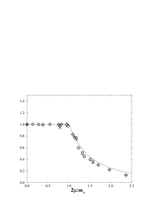
Figure 5: The chiral condensate versus $\mu/(m_{\pi}/2)$ for QCD with two colors in the adjoint representation (Figure taken from ref. [ [81]]).

Results for QCD with two colors in the fundamental representation obtained in [ [84]] are shown in Fig. 6. Again we find good agreement with the mean field results (90). Furthermore, if we plot the same data versus $m_{\pi}^{2}/4\mu^{2}$ the curve reminds us of the resolvent for QCD in phased quenched QCD after transforming the $z$ dependence of the resolvent at fixed $\mu$ into a $\mu$ dependence at fixed $z$ (see Fig. 4). Since the condensate can be interpreted as the electric field at the quark mass due to charges at the position of the eigenvalues we have no eigenvalues for $\mu>m_{\pi}/2$ and for a narrow strip along the $m_{\pi}^{2}/4\mu^{2}$ axis. In the remaining region the Dirac eigenvalues are distributed homogeneously. The absence of eigenvalues close to the $m_{\pi}^{2}/4\mu^{2}$ axis is a signature[ [87]] of $\beta_{D}=4$. Indeed, such behavior has been identified both numerically [ [87]] and analytically [ [77]].

Figure 6: The chiral condensate versus $\mu/(m_{\pi}/2)$ (upper) and versus $m_{\pi}^{2}/4\mu^{2}$ (lower). The dashed curves in the lower figure are drawn to guide the eye and in the lower figure they represent the mean field result (90) (Data points taken from ref. [ [84]]).

4.2 Beyond Mean Field

One of the recurring questions in the study of phase transitions is the stability of the mean field analysis. In the following, we carry out a next-to-leading order study of the second order phase transition found at the mean-field level. Additional details can be found in [ [15, 16]]. We will concentrate on the free energy of the Bose condensed phase close to the mean-field critical chemical potential $\mu_{c}=M/2$, with the leading order pion mass given by the GOR relation: $M^{2}=Gm_{\rm q}/F^{2}$.

The chiral Lagrangian (72) contains the two operators that have the lowest dimension in momentum space and that are invariant under local flavor transformations. There are, of course, many operators of higher dimension that fulfill these symmetry constraints. One has to introduce a systematic power counting to account for their relative importance [ [2]]. Our power-counting scheme is the same as the one used in chiral perturbation theory, extended to include the chemical potential: $p\sim\mu\sim M\sim\sqrt{m_{\rm q}}$, where $p$ is a Goldstone momentum. The leading order chiral Lagrangian contains all the operators of order $p^{2}$ that fulfill the symmetry constraints. The next-to-leading order chiral Lagrangian contains all suitable operators of order $p^{4}$. In general, for any $N_{f}$, there are ten such operators that contribute to the free energy. They are made out of traces of $\nabla_{\nu}\Sigma\nabla_{\nu}\Sigma^{\dagger}$ and of $M_{1}\Sigma^{\dagger}+M_{2}\Sigma$. The next-to-leading order chiral Lagrangian can be written as

$$L^{(4)}=\sum_{i=0}^{9}L_{i}{\cal O}_{i}.$$ (91)

At next-to-leading order, that is $p^{4}$, one has to take into account the one-loop diagrams from the leading-order chiral Lagrangian (72), as well as the tree diagrams from the next-to-leading order Lagrangian (91). In this perturbative scheme, three Feynman diagrams contribute to the free energy at next-to-leading order (see fig. 7).

file=freeEnOrder.eps,height=2cm,width=4.5cm

Figure 7: Feynman diagrams that enter into the free energy at next-to-leading order. The dot denotes the contribution from $L$ (72), and the boxed $4$ the contribution from $L^{(4)}$ (91). The order in the momentum expansion is also given under each diagram.

The one-loop diagram is divergent in four dimensions. The theory can be renormalized by introducing renormalized coupling constants

$$L_{i}\rightarrow L_{i}^{r}(\Lambda)+\gamma_{i}\left[\frac{1}{4}-\Gamma(-d/2)\right]\frac{\Lambda^{d-4}}{(4\pi)^{d/2}},$$ (92)

where $\Lambda$ is the renormalization scale and $\gamma_{i}$ are numbers that can depend $N_{f}$ [ [2, 15]]. The renormalization can be carried out order by order in the perturbation theory. It does not depend on the chemical potential [ [15]].

The main technical difficulty at next-to-leading order comes from the computation of the one-loop diagram in the Bose condensed phase: Some modes are mixed [ [12, 15]]. Because of this mixing, one-loop integrals may be quite complicated. However, we notice that the angle $\alpha$ that appears in (82) can be used as an order parameter of the Bose condensed phase. Since we want to study the free energy of that phase near the mean-field critical chemical potential $\mu_{c}=M/2$, it is sufficient to compute the one-loop integrals for small $\alpha$, and $\mu$ close to $M/2$. The free energy is then given by

$$\frac{\Omega}{M^{2}F^{2}}\sim{\rm cst}-\left(a_{2}+(2+a_{3})(\frac{\mu}{M}-\frac{1}{2})\right)\alpha^{2}+\left(\frac{1}{8}-a_{4}\right)\alpha^{4}+\dots$$ (93)

The coefficients $a_{i}$ come from the next-to-leading order corrections. They are numbers that can be expressed in terms of the renormalized coupling constants (92). Their general form is given by

$$a_{i}=\left(\sum_{k=0}^{9}b_{ik}L^{r}_{k}(\Lambda)-\frac{1}{32\pi^{2}}\sum_{k=0}^{9}b_{ik}\gamma_{k}\ln\frac{M^{2}}{\Lambda^{2}}\right)\frac{M^{2}}{F^{2}}.$$ (94)

They do not depend on the renormalization scale $\Lambda$ and can be evaluated from the $L^{r}_{K}$ which can in principle be obtained from lattice simulations. They are expected to be small (of the order of $0.05$ in 3-color QCD [ [2]]).

The free energy (93) can be analyzed in the same way as a Landau-Ginzburg model. The coefficient of $\alpha^{4}$ is positive. Therefore, there is a second order phase transition when the coefficient of $\alpha^{2}$ vanishes. We thus find that the critical chemical potential at next-to-leading order is given by

$$\mu_{c}=\frac{1}{2}M(1-a_{2})=\frac{1}{2}m_{\pi}^{\rm NLO},$$ (95)

where $m_{\pi}^{\rm NLO}$ is the mass of the Goldstones at next-to-leading order and at zero $\mu$. It is remarkable that the next-to-leading order shift in $\mu_{c}$ corresponds exactly to the next-to-leading order correction of $m_{\pi}$. At next-to-leading order, we therefore find a second order phase transition at half the mass of the lightest particle that carries a nonzero baryon charge.

We have also calculated the critical exponents at next-to-leading order in chiral perturbation theory and find that they are still given by their mean-field values [ [15]]. Since $d=4$ is the critical dimension beyond which mean field exponents become valid, this is not entirely surprising. From the form of the propagators, we conjecture that the critical exponents are given by mean-field theory at any (finite) order in perturbation theory.

In summary, we find that the next-to-leading order corrections are only marginal. The main picture obtained from the mean-field analysis is still valid at next-to-leading order: A second order phase transition at $\mu_{c}=m_{\pi}/2$ with mean-field critical exponents separates the normal phase from a Bose condensed phase.

4.3 Nonzero Temperature

At the one-loop level in chiral perturbation theory, the influence of the temperature on the second-order phase transition can also be studied [ [16, 88]]. In order to study the phase transition at nonzero $T$ and $\mu$, we compute the free energy of the Bose condensed phase close the critical chemical potential $\mu_{c}=m_{\pi}/2$ at $T=0$. The temperature dependence of the free energy is solely contained in the 1-loop diagram in fig. 7. Since we are only interested in the behavior of the free energy of the Bose condensed phase near the phase transition, it is sufficient to compute it for small $\alpha$, small $T$, and $\mu$ close to $m_{\pi}/2$. This procedure again leads to a free energy that can be analyzed as a usual Landau-Ginzburg model. The minimum of the free energy is given by

$$\frac{\partial\Omega}{\partial\alpha}=0\Rightarrow\left\{\begin{array}[]{l}\alpha=0\\ -c_{2}+c_{4}\alpha^{2}+c_{6}\alpha^{4}=0,\end{array}\right.$$ (98)

where $c_{i}$ are coefficients that can be computed exactly. For instance, we get that $c_{2}=(32\sqrt{2\pi^{3}}F_{\pi}^{2}-\zeta(\frac{3}{2})\sqrt{m_{\pi}T^{3}})^{2}$ for $N_{f}=2$ [ [16]]. We find that at

$$\mu_{\rm tri} = \frac{m_{\pi}}{2}+\frac{m_{\pi}^{3}}{6\sqrt{3}\zeta^{2}(3/2)F_{\pi}^{2}}\left(1-\frac{\zeta(1/2)\zeta(3/2)}{4\pi}\right)^{3/2},$$

$$T_{\rm tri} = 2m_{\pi}\frac{4\pi-\zeta(1/2)\zeta(3/2)}{3\zeta^{2}(3/2)},$$ (99)

both $c_{2}$ and $c_{4}$ vanish. Therefore, we find that the second-order phase transition line given by $c_{2}=0$, that is

$$\mu_{\rm sec}(T)=\frac{m_{\pi}}{2}+\frac{1}{32F_{\pi}^{2}}\sqrt{\frac{m_{\pi}^{3}T^{3}}{2\pi^{3}}}\zeta(3/2),$$ (100)

ends at $\mu_{\rm tri}$. For a larger chemical potential, the phase transition is of first order. The second-order phase transition line (100) is in complete agreement with the semi-classical analysis of a dilute Bose gas in the canonical ensemble. This phase diagram has been confirmed by lattice simulations [ [82, 85]].

5 Conclusions

Below $\Lambda_{\rm QCD}$ the QCD Dirac spectrum both at zero and at a sufficiently small nonzero chemical potential is described completely by a suitable chiral Lagrangian. Below the Thouless energy, i.e. the scale for which the Compton wavelength of the Goldstone bosons is equal to the size of the box, the Dirac spectrum can be obtained from the zero momentum part of this theory. This matrix integral can also be derived from a chiral Random Matrix Theory with the global symmetries of the QCD partition function. Therefore, below the Thouless energy, the correlations of QCD Dirac eigenvalues are given by chiral Random Matrix Theory. At nonzero chemical potential the Dirac eigenvalues are located inside a strip in the complex plane. Going inside this strip the chiral condensate rotates into a superfluid Bose-Einstein condensate. A very similar phase transition is found for any system with a chemical potential with the quantum numbers of the Goldstone bosons. We have discussed in detail the phase diagram for QCD with two colors. Because of the Pauli-Gürsey symmetry diquarks appear as Goldstone bosons in this theory. We have analyzed the phase diagram of this theory to one-loop order and have found a tricritical point in the chemical potential-temperature plane. All our results are in agreement with recent lattice QCD simulations.

5.1 Acknowledgments

Arkady Vainshtein is thanked for being a long lasting inspirational force of our field and the TPI is thanked for its hospitality. D.T. is supported in part by “Holderbank”-Stiftung and by NSF under grant NSF-PHY-0102409. This work was partially supported by the US DOE grant DE-FG-88ER40388.

References

- [1] S. Weinberg, Phys. Rev. Lett. 18 (1967) 188; Phys. Rev. 166 (1968) 1568; Physica A 96 (1979) 327.
- [2] J. Gasser and H. Leutwyler, Ann. Phys. 158 (1984) 142; J. Gasser and H. Leutwyler, Nucl. Phys. B 250 (1985) 465; H. Leutwyler, Ann. Phys. 235 (1994) 165.
- [3] J.J.M. Verbaarschot, Phys. Lett. B 368 (1996) 137.
- [4] H. Leutwyler and A.V. Smilga, Phys. Rev. D 46 (1992) 5607.
- [5] J.C. Osborn and J.J.M. Verbaarschot, Phys. Rev. Lett. 81 (1998) 268; Nucl. Phys. B 525 (1998) 738.
- [6] E.V. Shuryak and J.J.M. Verbaarschot, Nucl. Phys. A 560 (1993) 306.
- [7] J.J.M. Verbaarschot, Phys. Rev. Lett. 72 (1994) 2531.
- [8] D. Toublan and J. J. Verbaarschot, Int. J. Mod. Phys. B 15 (2001) 1404.
- [9] V.L. Girko, Theory of random determinants Kluwer Academic Publishers, Dordrecht, 1990.
- [10] M. A. Stephanov, Phys. Rev. Lett. 76 (1996) 4472.
- [11] J.B. Kogut, M.A. Stephanov, and D. Toublan, Phys. Lett. B 464 (1999) 183.
- [12] J.B. Kogut, M.A. Stephanov, D. Toublan, J.J.M Verbaarschot, and A. Zhitnitsky, Nucl. Phys. B 582 (2000) 477.
- [13] D. T. Son and M. A. Stephanov, Phys. Rev. Lett. 86 (2001) 592.
- [14] J. B. Kogut and D. Toublan, Phys. Rev. D 64 (2001) 034007.
- [15] K. Splittorff, D. Toublan and J. Verbaarschot, Nucl. Phys. B 620 (2002) 290.
- [16] K. Splittorff, D. Toublan and J. Verbaarschot, hep-ph/0204076.
- [17] J. B. Kogut, D. Toublan and D. K. Sinclair, Phys. Lett. B 514 (2001) 77. J. B. Kogut, D. Toublan and D. K. Sinclair, hep-lat/0205019.
- [18] T. Banks and A. Casher, Nucl. Phys. B 169 (1980) 103.
- [19] J.J.M. Verbaarschot, Phys. Lett. B329 (1994) 351.
- [20] A. Smilga and J. J. Verbaarschot, Phys. Rev. D51 (1995) 829.
- [21] P. H. Damgaard, Phys. Lett. B425 (1998) 151.
- [22] K. Zyablyuk, hep-ph/9911300.
- [23] E. Brézin, Lec. Notes Phys. 216 (1984) 115.
- [24] K. Efetov, Adv. Phys. 32 (1983) 53.
- [25] A. Morel, J. Physique 48 (1987) 1111.
- [26] J.J.M. Verbaarschot, H.A. Weidenmüller, and M.R. Zirnbauer, Phys. Rep. 129 (1985) 367.
- [27] C. Bernard and M. Golterman, Phys. Rev. D49 (1994) 486; C. Bernard and M. Golterman, hep-lat/9311070; M.F.L. Golterman, Acta Phys. Polon. B25 (1994).
- [28] M. F. Golterman and K. C. Leung, Phys. Rev. D 57 (1998) 5703.
- [29] J. Osborn, D. Toublan and J. Verbaarschot, Nucl. Phys. B540 (1999) 317.
- [30] P.H. Damgaard, J.C. Osborn, D. Toublan, and J.J.M. Verbaarschot, Nucl. Phys. B 547 (1999) 305.
- [31] B.L. Altshuler, I.Kh. Zharekeshev, S.A. Kotochigova and B.I. Shklovskii, Zh. Eksp. Teor. Fiz. 94 (1988) 343.
- [32] A. Garcia-Garcia and J. Verbaarschot, Nucl. Phys. B 586 (2000) 668; A. Garcia-Garcia and J. Verbaarschot, cond-mat/0204151.
- [33] S. Chandrasekharan and N. Christ, Nucl. Phys. B (Proc. Suppl.) 47 (1996) 527.
- [34] M.Á. Halász and J.J.M. Verbaarschot, Phys. Rev. Lett. 74 (1995) 3920; M.Á. Halász, T. Kalkreuter, and J.J.M. Verbaarschot, Nucl. Phys. B (Proc. Suppl.) 53 (1997) 266.
- [35] R. Pullirsch, K. Rabitsch, T. Wettig, and H. Markum, Phys. Lett. B 427 (1998) 119.
- [36] B.A. Berg, H. Markum, and R. Pullirsch, Phys. Rev. D 59 (1999) 097504.
- [37] R.G. Edwards, U.M. Heller, J. Kiskis, and R. Narayanan, Phys. Rev. Lett. 82 (1999) 4188.
- [38] R.G. Edwards, U.M. Heller, J. Kiskis, and R. Narayanan, Phys. Rev. Lett. 82 (1999) 4188.
- [39] P.H. Damgaard, R.G. Edwards, U.M. Heller, and R. Narayanan, Phys. Rev. D 61 (2000) 094503; Nucl. Phys. B (Proc. Suppl.) 47 (1996) 527.
- [40] M.E. Berbenni-Bitsch, S. Meyer, A. Schäfer, J.J.M. Verbaarschot, and T. Wettig, Phys. Rev. Lett. 80 (1998) 1146.
- [41] J.-Z. Ma, T. Guhr, and T. Wettig, Eur. Phys. J. A 2 (1998) 87.
- [42] P.H. Damgaard, U.M. Heller, and A. Krasnitz, Phys. Lett. B 445 (1999) 366.
- [43] M. Göckeler, H. Hehl, P.E.L. Rakow, A. Schäfer, and T. Wettig, Phys. Rev. D 59 (1999) 094503.
- [44] R. Edwards, U. Heller, and R. Narayanan, Phys. Rev. D 60 (1999) 077502.
- [45] M.E. Berbenni-Bitsch, S. Meyer, and T. Wettig, Phys. Rev. D 58 (1998) 071502.
- [46] F. Farchioni, I. Hip, C.B. Lang, and M. Wohlgenannt, Nucl. Phys. B 549 (1999) 364; Nucl. Phys. B (Proc. Suppl.) 73 (1999) 939.
- [47] M.E. Berbenni-Bitsch, A.D. Jackson, S. Meyer, A. Schäfer, J.J.M. Verbaarschot, and T. Wettig, Nucl. Phys. B (Proc. Suppl.) 63 (1998) 820.
- [48] P.H. Damgaard, U.M. Heller, R. Niclasen, and K. Rummukainen, Phys. Rev. D 61 (2000) 014501.
- [49] F. Farchioni, I. Hip, and C.B. Lang, Phys. Lett. B 471 (1999) 58; Nucl. Phys. B (Proc. Suppl.) 83-84 (2000) 482.
- [50] M. Schnabel and T. Wettig, hep-lat/9912057.
- [51] F. Farchioni, P. de Forcrand, I. Hip, C.B. Lang, and K. Splittorff, Phys. Rev. D 62 (2000) 014503.
- [52] P.H. Damgaard, U.M. Heller, R. Niclasen, and K. Rummukainen, hep-lat/0003021.
- [53] M.E. Berbenni-Bitsch, M. Göckeler, T. Guhr, A.D. Jackson, J.-Z. Ma, S. Meyer, A. Schäfer, H.A. Weidenmüller, T. Wettig, and T. Wilke, Phys. Lett. B 438 (1998) 14; M.E. Berbenni-Bitsch, M. Göckeler, S. Meyer, A. Schäfer, and T. Wettig, Nucl. Phys. B (Proc. Suppl.) 73 (1999) 605.
- [54] M.E. Berbenni-Bitsch, M. Göckeler, H. Hehl, S. Meyer, P.E.L. Rakow, A. Schäfer, and T. Wettig, Phys. Lett. B 466 (1999) 293; Nucl. Phys. B (Proc. Suppl.) 83-84 (2000) 974.
- [55] J.J.M. Verbaarschot and I. Zahed, Phys. Rev. Lett. 70 (1993) 3852.
- [56] D. Toublan and J. J. Verbaarschot, Nucl. Phys. B 603 (2001) 343.
- [57] F.J. Dyson, J. Math. Phys. 3 (1962) 140, 157, 166, 1199.
- [58] E. Brézin, S. Hikami, and A. Zee, Nucl. Phys. B 464 (1996) 411.
- [59] A. Jackson, M. Sener, J. Verbaarschot, Nucl. Phys. B 479 (1996) 707.
- [60] G. Akemann, P.H. Damgaard, U. Magnea, and S. Nishigaki, Nucl. Phys. B 487 (1997) 721.
- [61] A. Jackson, M. Sener, J. Verbaarschot, Nucl. Phys. B 506 (1997) 612.
- [62] T. Guhr and T. Wettig, Nucl. Phys. B 506 (1997) 589.
- [63] E. Kanzieper and V. Freilikher, Phys. Rev. Lett. 78 (1997) 3806; Phys. Rev. E 55 (1997) 3712; cond-mat/9809365.
- [64] M.R. Zirnbauer, J. Math. Phys. 37 (1996) 4986; F.J. Dyson, Comm. Math. Phys. 19 (1970) 235.
- [65] I. Barbour, N. Behihil, E. Dagotto, F. Karsch, A. Moreo, M. Stone and H. Wyld, Nucl. Phys. B275 (1986) 296; M.-P. Lombardo, J. Kogut and D. Sinclair, Phys. Rev. D54 (1996) 2303.
- [66] C. Baillie, K.C. Bowler, P.E. Gibbs, I.M. Barbour, and M. Rafique, Phys. Lett. B 197 (1987) 195.
- [67] H. Markum, R. Pullirsch, and T. Wettig, Phys. Rev. Lett. 83 (1999) 484.
- [68] I.M. Barbour, S.E. Morrison, E.G. Klepfish, J.B. Kogut, and M.-P. Lombardo, Nucl. Phys. (Proc. Suppl.) A 60 (1998) 220.
- [69] S. Hands, I. Montvay, S. Morrison, M. Oevers, L. Scorzato and J. Skullerud, Eur. Phys. J. C 17 (2000) 285.
- [70] K.B. Efetov, Phys. Rev. Lett. 79 (1997) 491; Phys. Rev. B 56 (1997) 9630.
- [71] J. Feinberg and A. Zee, Nucl. Phys. B 504 (1997) 579; Nucl. Phys. B 501 (1997) 643.
- [72] M. Alford, A. Kapustin and F. Wilczek, Phys. Rev. D 59 (1999) 054502.
- [73] D. Toublan and J. J. Verbaarschot, Nucl. Phys. B 560 (1999) 259.
- [74] J. Ginibre, J. Math. Phys. 6 (1965) 440.
- [75] Y. Fyodorov, B. Khoruzhenko, and H.-J. Sommers, Phys. Lett. A 226 (1997) 46; Phys. Rev. Lett. 79 (1997) 557; Ann. Ins. H. Poincaré, 68 (1998) 449.
- [76] P.J. Forrester, Phys. Rep. 301 (1998) 235.
- [77] A. V. Kolesnikov and K. B. Efetov, Waves Random Media 9 (1999) 71.
- [78] G. Akemann, Phys. Rev. Lett. 89 (2002) 072002; G. Akemann, hep-th/0204246; G. Akemann, hep-th/0206086.
- [79] A. Garcia-Garcia, S. Nishigaki and J. Verbaarschot, cond-mat/0202151.
- [80] S . Hands, J. B. Kogut, M. P. Lombardo and S. E. Morrison, Nucl. Phys. B 558 (1999) 327.
- [81] S. Hands, I. Montvay, S. Morrison, M. Oevers, L. Scorzato and J. Skullerud, Eur. Phys. J. C 17 (2000) 285.
- [82] J. B. Kogut, D. Toublan and D. K. Sinclair, Phys. Lett. B 514 (2001) 77.
- [83] J. B. Kogut and D. K. Sinclair, hep-lat/0202028.
- [84] J. B. Kogut, D. K. Sinclair, S. J. Hands and S. E. Morrison, Phys. Rev. D 64 (2001) 094505.
- [85] J. B. Kogut, D. Toublan and D. K. Sinclair, Phys. Lett. B 514 77 (2001).
- [86] R. Aloisio, A. Galante, V. Azcoiti, G. Di Carlo and A. F. Grillo, hep-lat/0007018.
- [87] M. Halasz, J. Osborn and J. Verbaarschot, Phys. Rev. D 56 (1997) 7059.
- [88] J. Gasser and H. Leutwyler, Phys. Lett. B 184 (1987) 83; Phys. Lett. B 188 (1987) 477; P. Gerber and H. Leutwyler, Nucl. Phys. B 321 (1989) 387; A. Schenk, Nucl. Phys. B 363 (1991) 97; D. Toublan, Phys. Rev. D 56 (1997) 5629.