SU-ITP 00-25

MIT-CTP-3295

hep-th/0208013

Disturbing Implications of a Cosmological Constant

L. Dyson^a,b, M. Kleban^a, L. Susskind^a

^aDepartment of Physics

Stanford University

Stanford, CA 94305-4060

^bCenter for Theoretical Physics

Department of Physics

Massachusetts Institute of Technology

Cambridge, MA 02139

In this paper we consider the implications of a cosmological constant for the evolution of the universe, under a set of assumptions motivated by the holographic and horizon complementarity principles. We discuss the “causal patch” description of spacetime required by this framework, and present some simple examples of cosmologies described this way. We argue that these assumptions inevitably lead to very deep paradoxes, which seem to require major revisions of our usual assumptions.

1 Recurrent Cosmology

As emphasized by Penrose many years ago, cosmology can only make sense if the world started in a state of exceptionally low entropy. The low entropy starting point is the ultimate reason that the universe has an arrow of time, without which the second law would not make sense. However, there is no universally accepted explanation of how the universe got into such a special state. In this paper we would like to sharpen the question by making two assumptions which we feel are well motivated from observation and recent theory. Far from providing a solution to the problem, we will be led to a disturbing crisis.

Present cosmological evidence points to an inflationary beginning and an accelerated de Sitter end. Most cosmologists accept these assumptions, but there are still major unresolved debates concerning them. For example, there is no consensus about initial conditions. Neither string theory nor quantum gravity provide a consistent starting point for a discussion of the initial singularity or why the entropy of the initial state is so low. High scale inflation postulates an initial de Sitter starting point with Hubble constant roughly $10^{-5}$ times the Planck mass. This implies an initial holographic entropy of about $10^{10}$, which is extremely small by comparison with today’s visible entropy. Some unknown agent initially started the inflaton high up on its potential, and the rest is history.

Another problem involves so-called transplanckian modes. The quantum fluctuations which seed the density perturbations at the end of inflation appear to have originated from modes of exponentially short wave length. This of course conflicts with everything we have learned about quantum gravity from string theory. The same problem occurs when studying black holes. In the naive free field theory of Hawking radiation, late photons appear to come from exponentially small wavelength transplanckian modes [1]. We now know that this is an artifact of trying to describe the complex interacting degrees of freedom of the horizon by quantum field theory defined on both the interior and exterior of the black hole. A consistent approach based on black hole complementarity [2] describes the black hole in terms of strongly interacting degrees of freedom of Planckian or string scale, and restricts attention to the portion of the space–time outside the horizon.

The late time features of a universe with a cosmological constant are also not well understood. The conventional view is that the universe will end in a de Sitter phase with all matter being infinitely diluted by exponential expansion. All comoving points of space fall out of causal contact with one another. The existence of a future event horizon implies that the objects that string theory normally calculates, such as S–Matrix elements, have no meaning [3]. In addition, there are questions of stability of de Sitter space which have been repeatedly raised in the past [4]. The apparent instabilities are due to infrared quantum fluctuations which seem to be out of control. Thus the final state is also problematic.

In our opinion both the transplanckian and the late time problems have a common origin. They occur because we try to build a quantum mechanics of the entire global spacetime–including regions which have no operational meaning to a given observer, because they are out of causal contact with that observer. The remedy suggested by the black hole analogue is obvious; restrict all attention to a single causal patch [28, 8, 9]. As in the case of black holes, the quantum description of such a region should satisfy the usual principles of quantum mechanics [2]. In other words, the theory describes a closed isolated box bounded by the observer’s horizon, and makes reference to no other region. Furthermore, as in the case of black holes, the mathematical description of this box should satisfy the conventional principles of linear unitary quantum evolution.

Perhaps the most important conceptual lesson that we have learned from string theory is that quantum gravity is a special case of quantum mechanics. Thus far every nonperturbative well-defined formulation of string theory involves a hamiltonian, and a space of states for it to act on. This includes matrix theory and all the versions of AdS/CFT. The question of this paper is whether the usual rules apply to cosmology, and can they explain, or at least allow, the usual low entropy starting point. In the following we will assume the usual connections between quantum statistical mechanics and thermodynamics.

These assumptions–together with the existence of a final cosmological constant–imply that the universe is eternal but finite. Strictly speaking, by finite we mean that the entropy of the observable universe is bounded, but we can loosely interpret this as saying the system is finite in extent. On the average it is in a steady state of thermal equilibrium. This is a very weak assumption, because almost any large but finite system, left to itself for a long enough time, will equilibrate (unless it is integrable) [22]. However, intermittent fluctuations occur which temporarily disturb the equilibrium. It is during the return to equilibrium that interesting events and objects form.

The essential point can be illustrated with an analogy. Instead of the universe, let’s consider a sealed box full of gas molecules. Start with a particular low entropy initial condition with all the molecules in a very small volume in one corner of the box. The molecules are so dense that they form a fluid. When released the molecules flow out from the corner and eventually fill the box uniformly with gas. For some time the system is far from equilibrium. During this time, the second law insures that the entropy is increasing and interesting things can happen. For example, complex “dissipative structures” such as eddy flows, vortices, or even life can form. Eventually the system reaches equilibrium, and all structures disappear. The system dies an entropy death. This is the classical hydrodynamic description of the evolution of a “universe”. But this description is only correct for time intervals which are not too long.

Let $S$ be the final thermodynamic entropy of the gas. Then on time scales of order

$$T_{r}\sim\exp{S}$$ (1.1)

the system will undergo Poincare recurrences [8, 9]. Such a recurrence can bring all the particles back into the corner of the room. On such long time scales the second law of thermodynamics does not prevent rare events, which effectively reverse the direction of entropy change. Obviously, the recurrence allows the entire process of cosmology to begin again, although with a slightly different initial condition. What is more, the sequence of recurrences will stretch into the infinite past and future. The question then is whether the origin of the universe can be a naturally occurring fluctuation, or must it be due to an external agent which starts the system out in a specific low entropy state? We will discuss this in greater detail in Section 6.

2 The AdS Black Hole as a Cosmology

It has been widely suggested that the study of cosmology has close similarity with the study of the interior of black holes. In this paper we will outline a framework for cosmology which is partly inspired by the analysis of AdS/Schwarzschild black holes [18]. This system, although unrealistic as a cosmology, is extremely well understood through the AdS/CFT duality.

The relevant static metric, suitably normalized, is

$$ds^{2}=\left(r^{2}+1-{b_{D}\over r^{D-3}}\right)dt^{2}-\left(r^{2}+1-{b_{D}\over r^{D-3}}\right)^{-1}dr^{2}-r^{2}d\Omega^{2},$$ (2.1)

where $d\Omega^{2}$ represents the metric of a unit $D-2$ sphere and $b_{D}$ depends on the $D$-dimensional Newton constant and the volume of the $D-2$ sphere. The horizon is located at $r_{+}$, the largest solution to the equation

$$r^{2}+1-{b_{D}\over r^{D-3}}=\ 0.$$ (2.2)

The boundary is at $r=\infty$. In general this geometry will be accompanied by a compact factor such as a 5-sphere for the case of ${\rm AdS}_{5}$. We will refer to the boundary as the “observer.” Observations by the observer are known to be completely described by a unitary holographic quantum mechanics with no loss of information. Furthermore the black hole from the observer’s viewpoint is just the thermal state of the holographic dual.

Figure 1: An eternal AdS Schwarzshild black hole, or de Sitter space. The horizontal boundaries are space-like singularities in the case of the AdS black hole, and the infinitely inflated past and future in the case of de Sitter.

Now consider the classical global geometry represented by a Penrose diagram as shown in figure (1). It is evident from the diagram that the classical geometry can be interpreted as a cosmology. To the observer at the boundary, the entire universe can be described by the triangle in figure(2)

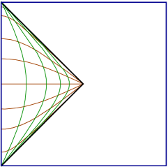
Figure 2: The causal patch for an observer at the boundary of an AdS Schwarzschild black hole, or in de Sitter space.

which we can call the causal patch. It describes the exterior of the black hole, defined by $r>r_{+}$. This region is described by a thermal density matrix in the exact holographic quantum theory. From the bulk viewpoint the Bekenstein entropy is the entropy of the causal patch.

On the other hand, the global geometry is more or less similar to closed FRW cosmologies. It starts with a big bang singularity and ends with a final crunch. An observer at the spatial center of the diagram will experience the crunch in a finite time. One peculiar feature is that the rapid time dependence near the early singularity is far from adiabatic. Under these kind of circumstances there should be large amounts of entropy production. On the other hand the geometry is obviously time symmetric. This is very unnatural and presumably means that the universe starts in very special, extremely fine tuned state. A rough analogy would be a history in which all the particles in a box start in one corner and after a given long time return to the corner. Such trajectories will exist but they are extremely unstable. Moving one particle a little bit will change the outcome to a more thermodynamically sensible final state.

A more reasonable cosmology can result if we started with a far from equilibrium configuration. For example, an initially empty AdS space of zero entropy could be excited by an infalling shell of energy originating at the boundary. From the dual conformal field theory point of view, this corresponds to varying the hamiltonian in a time dependent way. For example, by varying the gauge theory coupling a coherent pulse of dilaton wave can be injected into the bulk. The ability to modify the action in this way and still have a solution to the supergravity equations of motion is of course connected with the existence of an ultraviolet boundary.

The dilaton pulse will create some thermal energy. If it has enough energy, an AdS black hole will form. The observer in the bulk will start life in empty AdS with zero entropy. He will then see some sudden time dependence as the dilaton wave passes. Afterwards the bulk will become excited with heat and particles and possibly dissipative structures. Eventually the bulk observer will be destroyed at the singularity. This cosmology is shown in figure (3).

Figure 3: An AdS black hole created by an infalling shell of energy originating at the boundary.

From the CFT side, the black hole formation is just the classical gravitational description of the approach to thermal equilibrium.

As in the case of the box of molecules, this description does not make sense for time intervals of order $\exp{S}$. Poincare recurrences will lead to intermittent rare fluctuations in which the energy of the black hole reassembles itself into an energy shell, which goes out and then reflects back. In other words, the formation of the black hole will endlessly repeat itself at intervals of order $T_{r}\sim\exp{S}$. Each recurrence will be different in its microscopic details from the previous.

One important fact is that these recurrences cannot be described by classical general relativity. It is as though classical relativity–with its thermodynamic-like laws of black hole mechanics–is a coarse grained version of a more detailed theory. This raises the obvious question of whether the initial conditions of the universe could have originated from a Poincare recurrence; that is, a large thermal fluctuation to a very low entropy configuration.

In the recurrent view of cosmology the second law of thermodynamics and the arrow of time would have an unusual significance. In fact they are not laws at all. What is true is that interesting events, such as life, can only occur during the brief out-of-equilibrium periods while the system is returning to equilibrium. In other words, the second law and the existence of a time arrow are anthropic. They are part of the environmental conditions needed for life.

3 Thinking Inside The Box

For reasons that have been explained in many places, if we want to apply the ordinary principles of unitary quantum mechanics to a system with horizons, we need to restrict attention to the region on the observer’s side of the horizon. For example, the triangle of figure (2) is the the region appropriate to an observer on the left-hand boundary of the space. We call such a region the $observer^{\prime}s\ \ causal\ \ patch$.

The space that we will consider next is de Sitter space. The causal structure of de Sitter space is described by the same Penrose diagram as shown in figures (1) and (2), but with different interpretations. The horizontal boundaries which previously described singularities now represent the infinitely inflated past and future (IIP and IIF). The vertical edges are no longer true boundaries, as they were in AdS, but represent observers at opposite poles of a global spatial sphere. The triangle of figure (2) is now the causal patch of one observer. One point in common with the AdS black hole is that the causal patch is described thermodynamically. The entropy usually ascribed to de Sitter space is that of the causal patch. As in the black hole case, it is the logarithm of the number of effective quantum states of the thermal ensemble. More exactly it is ${\rm Tr}\rho\log{\rho}$, where $\rho$ is the density matrix describing the causal patch.

The causal patch can be described by a static metric

$$ds^{2}=R^{2}\left[(1-r^{2})dt^{2}-(1-r^{2})^{-1}dr^{2}-r^{2}d\Omega^{2}\right],$$ (3.1)

where $R$ is the inverse Hubble scale. The radial coordinate runs from $r=0$ at the location of the observer to $r=1$ at the horizon. The horizon is the boundary of a kind of box or cavity with the observer at the center. Because the boundary of the box is a horizon, the box has a finite temperature and entropy:

$$T = {1\over 2\pi R}$$ (3.2)

$$S = {4\pi R^{2}\over 4G}.$$ (3.4)

We are interested not only in the classical description of “dead” de Sitter space, but also the non-equilibrium fluctuations that can lead to an interesting universe. In order to illustrate the main ideas, we will study a simplified model in which the universe will be taken to be $(2+1)$ dimensional, so that $\Omega$ in (3.1) is replaced by a single angle $\theta$. Furthermore, we will restrict discussion to configurations with rotational symmetry and no angular motion.

Our first task is to generalize the metric in (3.1) to non-static configurations. In particular, we want to introduce coordinates which cover only the region in full causal contact with the observer at $r=0$. By this we mean the region which can both receive signals from, and transmit signals to, the observer. To accomplish this, it is convenient to first change the radial coordinate in (3.1) so that the metric has the form

$$ds^{2}=e^{v}(dt^{2}-d\rho^{2})-Z^{2}d\theta^{2}.$$ (3.5)

The transformation for pure de Sitter space is given by:

$$r = \tanh{{\rho\over R}}$$ (3.6)

$$e^{v} = {1\over\cosh^{2}{{\rho\over R}}}$$ (3.8)

$$Z = R\tanh{{\rho\over R}}.$$ (3.10)

The entire causal patch is covered by the region $\rho\geq 0,\ \ -\infty<t<+\infty.$

Now let us introduce a gauge fixing procedure which leads to coordinates of this type, for arbitrary geometries of the form we are considering. In $(2+1)$ dimensions we can choose three gauge fixing conditions. We choose these to be

$$g_{tt} = -g_{rr}$$ (3.11)

$$g_{tr} = 0$$ (3.12)

$$g_{r\theta} = 0.$$ (3.13)

In addition, given the conditions of rotational symmetry and no angular velocity, the component $g_{t\theta}$ vanishes. Thus the metric has the form (3.5). However we have not used all the gauge fixing freedom at our disposal. Let us define coordinates $t^{(\pm)}=t\pm\rho$. Conformal transformations of the form $X^{\pm}=X^{\pm}(t^{\pm})$ preserve the form of the metric. This means we can still choose two functions, each of one variable. Thus we make the additional gauge choices

$$e^{v}|_{\rho=0} = 1$$ (3.14)

$$Z|_{\rho=0} = 0.$$ (3.16)

This completely fixes the gauge, and results in coordinates which exactly cover the causal patch of the observer at $\rho=0$ .

We could also choose to fix the guage by requiring regularity in the coordinates at the horizon, rather than at the origin. Once the observer’s location in the infinite past and future are chosen, the causal patch horizon is determined, and therefore such a gauge choice is manifestly independent of the observers trajectory. Furthermore, it is the appropriate choice if one wishes to define a fluctuating energy. As we will see, fixing the gauge at the origin makes the energy independent of the de Sitter radius.

In general, $e^{v}$ and $Z$ will be time dependent. An important point is that at the location of the observer, the coordinate $t$ is precisely the proper time of a clock carried by the observer. We will call this gauge the observocentric-gauge, or O-gauge. The coordinates $t,\rho$ can easily be constructed for some special cases of interest. In particular, consider a closed FRW metric

$$ds^{2}=dT^{2}-a(T)^{2}\left[d\theta^{2}+\sin^{2}(\theta)d\phi^{2}\right],$$ (3.17)

which begins in the remote past as a de Sitter space with radius $R^{\prime}$ and ends in the remote future as a de Sitter space with radius $R$. An inflationary universe with a final nonzero cosmological constant is an example. The scale factor $a$ is a function only of FRW time $T$. To construct the O-gauge coordinates $\rho$ and $t$ at an arbitrary spacetime point $p$, consider past and future light rays originating at $p$ and propagating to the observer. These intersect the observer’s trajectory at past and future FRW times $T_{\pm}$. The O-gauge coordinates of the point $p$ are then

$$2t = T_{+}+T_{-}$$ (3.18)

$$2\rho = T_{+}-T_{-}.$$ (3.19)

It is also easy to find the values of $e^{v}$ and $Z$. Define the function $\tau(x)=\int^{x}dT/a(T)$, its inverse $\tau^{-1}$, and $t_{\pm}=t\pm\rho$. Then

$$e^{v} = {a^{2}\left(\tau^{-1}\left({1\over 2}\left[\tau(t_{+})+\tau(t_{-})\right]\right)\right)\over a(t_{+})a(t_{-})}$$ (3.20)

$$Z = a^{2}\left(\tau^{-1}\left({\tau(t_{+})+\tau(t_{-})\over 2}\right)\right)\sin^{2}\left({\tau(t_{+})-\tau(t_{-})\over 2}\right).$$ (3.22)

One can easily represent spatially flat inflationary universes in a similar manner; in general, the O-gauge coordinates are constructed so as to exactly cover the observer’s causal patch. The time variable at $\rho=0$ (the observer) is always proper time. The construction can be generalized to include non-rotationally invariant geometries, in arbitrary dimension. Although we will not discuss this in detail here, one would construct the causal patch coordinates simply by considering the intersection of the future and past lightcones of two points $\tau_{\pm}$ along the trajectory. These will intersect along a $d-2$ sphere of constant $t$ and $\rho$, as given by 3.19.

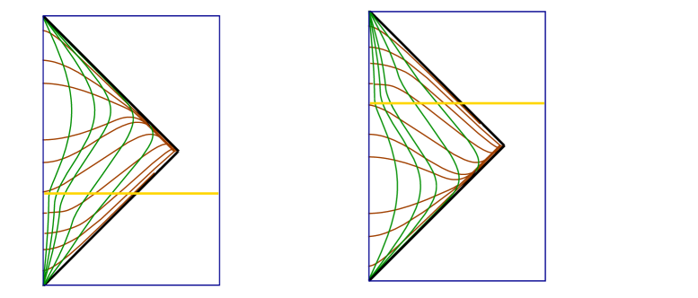
Figure 4: The causal patch for two types of global time transitions from one de Sitter space to another.

There are two cases that can be distinguished by the “height” of the Penrose diagram. If the height is less than twice the width, as in the two spacetimes of figure (4), then the surfaces $t=\pm\infty$ intersect within the diagram at a Rindler type horizon, just as they would in de Sitter space. If, however, the diagram is taller than twice its width, as in figure (5),

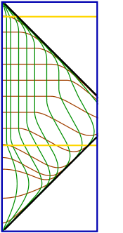
Figure 5: A transition from a de Sitter space with a small radius of curvature to a matter dominated phase, followed by a transition to a large de Sitter. In this example, the horizon is pushed all the way around to the south pole of the sphere, and vanishes for intermediate times.

the two surfaces terminate at the antipodal point before intersecting. In this case the spatial slices $t=const$ form closed spatial spheres. In either case, the surfaces $t=\pm\infty$ are the past and future horizons of the observer.

It is also convenient to stretch the horizon in a way familiar from black hole physics. One way to do this is to define a time-like surface as follows: begin either at the intersection of the past and future horizons, or at the point where the spatial surfaces meet the antipode. From that point work back (toward $\rho=0)$ along the surfaces of constant $t$ a fixed proper distance of order the Planck or string scale. The resulting position is the stretched horizon.

For the case in which the geometry begins and ends in de Sitter phases, the stretched horizons at early and late times are the same as we would expect for the corresponding eternal de Sitter spaces. This implies that the horizon entropy within the causal patch in the far future and past is bounded in the ordinary way. In particular, no matter how many e-foldings of inflation occur before the spacetime exits to its final configuration, the entropy in the final patch must still be bounded by the area of the horizon, as determined by the cosmological constant. This bound can easily be shown to be equivalent to the covariant entropy bound as proposed in [30].

4 Some Examples

Here are some examples of thinking inside the box. Let’s begin with a minimally coupled scalar field coupled to gravity. The action is given by

$$I=\int d\rho d\theta dt\sqrt{-g}\left(R+g^{\mu\nu}\partial_{\mu}\phi\partial_{\nu}\phi-V(\phi)\right).$$ (4.1)

In the O–gauge the action is

$$I=\int d\rho d\theta dt\left(\dot{Z}\dot{v}-Z^{\prime}v^{\prime}+Z(\dot{\phi}^{2}-(\phi^{\prime})^{2})-e^{v}ZV(\phi)\right).$$ (4.2)

It is straightforward to construct a Hamiltonian from this action. Its value is given by

$$H=\int d\rho d\theta\left(\dot{Z}\dot{v}+Z^{\prime}v^{\prime}+Z(\dot{\phi}^{2}+(\phi^{\prime})^{2})+e^{v}ZV(\phi)\right).$$ (4.3)

Classically the value of $H$ is constrained by the Einstein equations. The time–time component is given by

$$\dot{Z}\dot{v}+Z^{\prime}v^{\prime}+Z(\dot{\phi}^{2}+(\phi^{\prime})^{2})+e^{v}ZV(\phi)-2Z^{\prime\prime}=0.$$ (4.4)

By integrating this equation over all space we find

$$H-2\partial_{\rho}Z|^{\rho=\infty}_{\rho=0}=0.$$ (4.5)

The boundary contribution at $\rho=\infty$ vanishes in general, and for geometries which are smooth at the origin, $\partial_{\rho}Z=1$. Thus the constraint requires $H=2$. As mentioned above, this is completely independent of the de Sitter curvature, and of any non-singular matter content in the spacetime (had we chosen to fix the guage at the horizon, the energy would depend on the far past and future values of the de Sitter curvature). Therefore, complicated dynamical processes such as the evolution from a small de Sitter space to a large one, with some periods of matter or radiation domination in between, can all occur at constant energy. We will illustrate this point with some specific examples below.

Solutions can easily be generated from FRW solutions transformed into the O–gauge. As an example, we take the potential $V$ to be a constant plus a small step-like function:

$$V(\phi)=V-c\tanh{L\phi},$$ (4.6)

with $c<<V$. There are solutions which in FRW coordinates roll from negative to positive $\phi$, going over the step at some fairly localized time. This time can be either during the contracting or the expanding phase of the FRW description. Roughly speaking there is a small decrease of the cosmological constant at this time. The change is small so the back reaction on the geometry is also small.

In O–coordinates, the behavior depends on whether the transition occurs during FRW contraction or expansion. In the former case, a domain wall or wave of decreased cosmological constant originates at the horizon ($\rho=\infty$) and propagates inward toward the observer. Energy is released, and since the final entropy of the horizon increases, we may describe the domain wall as producing entropy which falls to the horizon.

In the latter case that the transition occurs during expansion, the O–description is quite different. In this case the domain wall originates at the observer and falls toward the horizon. Again the final effect is to increase the horizon entropy.

The back reaction on the geometry is small, but it results in making the Penrose diagram slightly taller. The effect is to push the horizon point slightly toward the antipodal point as in figure (4). To understand this effect, first consider the causal patch in pure de Sitter space. The patch is perfectly static and consists of a hemisphere (southern). The observer is at the south pole. The horizon is at the equator, and stretching it displaces it slightly south.

In the time dependent solution the stretched horizon begins in the past at its static location but then temporarily moves away from the observer toward the north pole. Eventually it returns to very near the equator.

One can also study the more extreme case in which there is a very large change in the cosmological constant, as in a realistic inflationary theory. Typically, in this case, the horizon intersection moves far toward the north pole. In some cases it may even reach the pole, so that the causal patch may temporarily become a closed sphere, with the horizon disappearing for a time. We illustrate an example of this in figure (5).

As another example of thinking in the box, consider a mass distribution in de Sitter space. For simplicity, we will work with a spherically symmetric matter distribution localized along a thin ring. The solution outside of the ring will have a deficit in the range of the angular variable. The solution can be written

$$ds^{2}=R^{2}\left[(1-r^{2})dt^{2}-(1-r^{2})^{-1}dr^{2}-\alpha^{2}r^{2}d\theta^{2}\right]\hskip 30.0pt(r<r_{0})\ .$$ (4.7)

where $r_{0}$ is the position of the ring, $\theta\simeq\theta+2\pi$ and $0<\alpha\leq 1$ determines the deficit angle. Note that the area of the horizon is $2\pi\alpha\leq 2\pi$. We interpret this as meaning that some of the degrees of freedom making up the horizon are “used up” in forming the ring. If the size of the ring is much smaller than the de Sitter radius, we can think of it as an object which could exist in the corresponding theory without a cosmological constant. In that case it is natural to identify the deficit angle with the mass. Evidently then, the mass is proportional to the amount of entropy used up in making the object. More precisely, the number of degrees of freedom borrowed from the stretched horizon is the product of the mass and the de Sitter space radius.

Inside the ring, the solution is pure de Sitter space with no deficit angle. The metric is

$$ds^{2}=R^{2}\left[(1-r^{\prime 2})dt^{\prime 2}-(1-r^{\prime 2})^{-1}dr^{\prime 2}-r^{\prime 2}d\theta^{2}\right]\hskip 30.0pt(r^{\prime}<r^{\prime}_{0})\ .$$ (4.8)

The condition that the metric be continuous across $r=r_{0}$ requires $r^{\prime}=\beta r+r_{0}(\alpha-\beta)$ and $t\ ^{\prime}=\beta^{-1}t$, with $\beta^{2}=(1-\alpha^{2}r_{0}^{2})(1-r_{0}^{2})^{-1}$ and $r^{\prime}_{0}=\alpha r_{0}$.

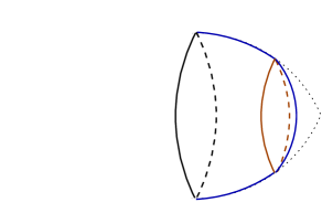
Figure 6: Cigar diagram for a ring mass in de Sitter space. The left-hand boundary is the horizon. The dotted line indicates the shape for the case of a point mass at the origin.

One can compute the stress-energy required for this solution to exist. The contribution from the ring is

$$\sqrt{g}T^{t}_{t}=\sqrt{1-r_{0}^{2}}\left(\alpha\sqrt{1-r_{0}^{2}}-\sqrt{1-\alpha^{2}r_{0}^{2}}\right)\delta(r-r_{0}),$$ (4.9)

and

$$\sqrt{g}T^{\theta}_{\theta}=\alpha r_{0}^{2}\left(1-\alpha\sqrt{(1-r_{0}^{2})(1-\alpha^{2}r_{0}^{2})^{-1}}\right)\delta(r-r_{0}).$$ (4.10)

This corresponds to a positive energy density in the ring (for $\alpha>0$), with some tension to hold it static. This solution is unstable to non-spherically symmetric perturbations, but this is not important for our purposes.

By making the appropriate coordinate transformations (3.10), we can easily express the above solution in O-gauge (3.5). The energy of the configuration then is given by (4.5), $H=2$. This solution makes manifest that the energy is independent of the matter content of the space. The time-time component of Einstein’s equations always contains second derivative terms, and we define energy by the boundary terms corresponding to these. In $2+1$ dimensions there are two possible contributions: at the origin and at the horizon. As we have already discussed, the contribution at the horizon generally vanishes. Very close to the origin the metric looks flat, and $Z\sim\rho$ as long as the mass distribution is not localized there. Since $\partial_{\rho}Z=1$, the energy is independent of the matter content of the space.

As the simple examples above show, a fluctuation which removes some degrees of freedom from the horizon (thereby decreasing its entropy), and deposits them in some configuration in the bulk of the space–perhaps by increasing the vacuum energy, or in the form of matter or radiation–is an energy conserving process. The observable history of the universe is one such fluctuation, occurring at fixed energy in some background de Sitter space.

5 Complementarity and its Implications

At this point we will add one more assumption, which is motivated by the success of string theory in describing black holes using the standard principles of quantum mechanics. The additional ingredient is the analog of black hole complementarity. In more general contexts it can be called Horizon Complementarity. We assume that the physics within the causal patch is exactly described by a dual quantum system that includes a Hamiltonian $H$ and a space of quantum states. Furthermore the state of the world within the causal patch is density matrix $\exp{(-\beta H)}$ with the appropriate temperature. The assumption is motivated by what we now know about other quantum gravity systems such as the AdS black hole .

We know a few things about the dual quantum system. From the fact that the entropy is finite, it follows that the energy levels are discrete and that the number of levels below any given energy is finite. That is all we really need, but there is also reason to believe that there may be an upper bound on the energy levels [28]. One way to argue this point is to observe that in other holographic dual theories, the UV sector of the theory is identified with the timelike boundary of the space. In the de Sitter case, the closest analog of a timelike boundary is the line $r=0$, suggesting that the high-energy degrees of freedom are sparse or non-existent above a certain level. By contrast, the low energy degrees of freedom are associated with the horizon of the causal patch. Since the area of the horizon at $r=1$ is larger than at any other radius, we expect the system to be very rich in low energy degrees of freedom. If this is correct, the quantum dual could be a system with a finite dimensional Hilbert space as advocated by Banks [6] and Fischler [7].

The implications of Horizon Complementarity are profound, and may lead to new cosmological questions and puzzles. As we shall see, it implies that the universe has neither a beginning nor and end. Instead, it intermittently recycles itself, but in a way that is very different from so called cyclic universes.

For our present purposes, Horizon Complementarity will be taken to mean that physics in the causal patch can be described in terms of a closed or isolated system described by conventional quantum mechanics. Furthermore we assume that the maximum entropy that the system can ever have is given by the entropy of a de Sitter space, whose size is determined by the cosmological constant. By the cosmological constant, we mean the true minimum value of the vacuum energy, not the value during early inflation. For illustrative purposes we can take the cosmological constant to be the current value of the dark energy that appears to be accelerating the expansion of the universe today. Horizon Complementarity then says the universe is described by any observer as a closed and finite system.

The implication of such a description, as we have suggested in Section (1), is that Poincare recurrences are inevitable. Starting in a high entropy, “dead” configuration, if we wait long enough, a fluctuation will eventually occur in which the inflaton will wander up to the top of its potential, thus starting a cycle of inflation, re–heating, conventional cosmology and heat death. The frequency of such events is very low. The typical time for a fluctuation to occur is of order

$$T_{r}\sim\exp{(S-S^{\prime})}$$ (5.1)

where $S$ is the equilibrium entropy and $S^{\prime}$ is the entropy of the fluctuation. The fluctuations we have in mind correspond to early inflationary eras during which the entropy is probably of order $10^{10}$, while the equilibrium entropy is of order $10^{120}$. Thus

$$T_{r}\sim\exp{10^{120}}.$$ (5.2)

This seems like an absurdly big time between interesting events, which by comparison last for a very short time. Nevertheless dismissing such long times as “unphysical” may be a symptom of extreme temporal provincialism.

Given our assumptions, the conclusion that such Poincare recurrences of the universe occur is unavoidable. The potential difficulty is not the long time between them, but rather that there may be far more probable ways of creating livable (“anthropically acceptable”) environments than those that begin high up on the inflationary potential (to height $V$).

In the next section, we will discuss the probability that a recurrence will lead to a world which is consistent with our own universe. First, however, there is an alternative that we should explore. It is suggested by the discussion of the AdS/Schwarzschild black hole in section (2) where the eternal black hole was replaced by a black hole formed from a shell of energy that originated at the boundary. From the dual point of view the system corresponds to a time dependent deformation of the boundary conformal field theory which heats the system. The question is whether a similar story makes sense for de Sitter space? We think the answer in no. The reason is that the causal patch does not have the analog of an ultraviolet boundary. Because AdS has such a boundary it is possible to modify the boundary conditions without changing the fact that the bulk theory still satisfies the bulk field equations. Without such a boundary there is no way to do the same for de Sitter space. Thus, if there is a theory of de Sitter space and its fluctuations we do not expect to be able to intervene from the outside and create a particular initial condition. In our view, the only possible origin of an out-of-equilibrium initial state is a large fluctuation.

We will conclude this section with a few remarks about the proposed dS/CFT duality that has been the subject of several recent papers. The idea is to use the space-like boundary of de Sitter space in place of the time-like boundary of AdS in order to formulate a holographic theory. In particular deformations of the boundary conditions at past infinity could allow us to introduce initial conditions such as an inflationary era. While this is an attractive idea, it does not seem consistent with the thermal properties of de Sitter space. To understand why, we can try to interpret the idea in the box. For a perturbation on the past boundary to influence the causal patch, the signal must pass through the past horizon of the observer. However the past horizon is just the infinite past $t=-\infty$. In other words, it simply corresponds to a perturbation of the box at infinitely negative time. Obviously, any such perturbation of a finite entropy thermal cavity will re-thermalize after a finite time. In fact, at any finite time, an infinite number of Poincare recurrences have already occurred.

6 The Misanthropic Universe?

Certainly, given enough time and a suitable inflaton, recurrences will eventually bring the box to a configuration that could serve as an initial starting point for a standard inflationary theory. The entropy of such configurations is very low. In a typical high-scale inflationary theory, the entropy of the initial de Sitter-like space can be as low as $10^{10}$. The entropy of the final de Sitter space (assuming the observed value for the dark energy) is of order $10^{120}$.

Inflationary starting points are very rare in time. That in itself is not a problem. Most of the rest of time during which nothing interesting is happening can, from an anthropic point of view, be thrown away. We can also throw away large fluctuations which lead to un–livable conditions. The danger is that there are too many possibilities which are anthropically acceptable, but not like our universe.

Let us consider the entropy in observable matter in today’s universe. It is of order $10^{100}$. This means that the number of microstates that are macroscopically indistinguishable from our world is $\exp{(10^{100})}$. But only $\exp{(10^{10})}$ of these states could have evolved from the low entropy initial state characterizing the usual inflationary starting point. The overwhelming majority of states which would have evolved into a world very similar to ours did not start in the usual low entropy ensemble.

To understand where they came from, imagine running these states backward in time until they thermalize in the eventual heat bath with entropy $10^{120}$. Among the vast number $\sim\exp{(10^{120})}$ of possible initial starting points, a tiny fraction $\sim\exp{(10^{100})}$ will evolve into a world like ours. However, all but $\sim\exp{(10^{10})}$ of the corresponding trajectories (in phase space) are extremely unstable to tiny perturbations. Changing the state of just a few particles at the beginning of the trajectory will lead to completely different states. Nevertheless, there are so many more of these configurations among the $\exp{(10^{120})}$ possible starting points that in a theory that relies on statistical likelyhood to fix the initial conditions, they completely dominate.

What is worse is that there are even more states which are macroscopically different than our world but still would allow life as we know it. As an example, consider a state in which we leave everything undisturbed, except that we replace a small fraction of the matter in the universe by an increase in the amount of thermal microwave photons. In particular, we could do this by increasing the temperature of the CMB from $2.7$ degrees to $10$ degrees. Everything else, including the abundances of the elements, is left the same. Naively one might think that this is impossible; no consistent evolution could get to this point since the extra thermal energy in the early universe would have destroyed the fragile nuclei. But on second thought, there must be a possible starting point which would eventually lead to this “impossible” state. To see this, all we have to do is run the configuration backward in time. Either classically or quantum mechanically, the reverse evolution will eventually lead back to a state which looks entirely thermal, but which, if run forward, will lead us back to where we began. In a theory dependent on Poincare recurrences, there would be many more “events,” in which the universe evolves into this modified state. Thus it would be vastly more likely to find a world at $10$ degrees with the usual abundances than in one at $2.7$ degrees. All of these worlds would be peculiar. The helium abundance would be incomprehensible from the usual arguments. In all of these worlds statistically miraculous (but not impossible) events would be necessary to assemble and preserve the fragile nuclei that would ordinarily be destroyed by the higher temperatures. However, although each of the corresponding histories is extremely unlikely, there are so many more of them than those that evolve without “miracles,” that they would vastly dominate the livable universes that would be created by Poincare recurrences. We are forced to conclude that in a recurrent world like de Sitter space  our universe would be extraordinarily unlikely.

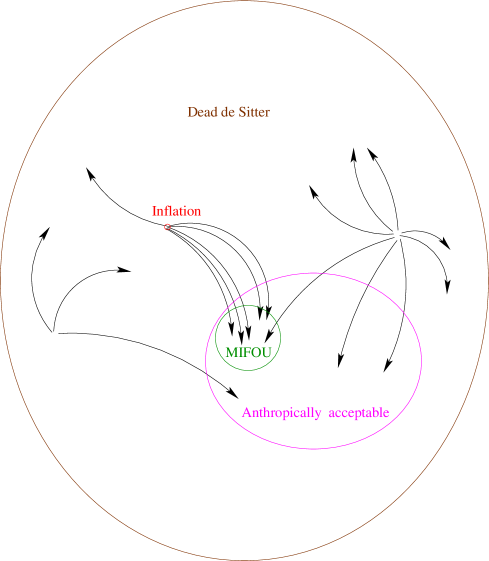
Figure 7: A schematic representation of the phase space of a universe with a cosmological constant. The vast majority of the space consists of states which are macroscopically “dead de Sitter;” that is, nearly empty de Sitter containing only some thermal radiation. A tiny subset of the states are anthropically acceptable, meaning that they contain complex structures such as stars and galaxies, and a very small subset of those are macroscopically indistinguishable from our universe (labelled MIFOU in the figure). Inflationary initial conditions occupy an even smaller fraction of the space. Trajectories which pass through the inflationary patch will almost always lead immediately to the MIFOU region, “mixing” into it in a “porous,” phase-space-area-preserving manner. The vast majority of the points in the MIFOU region did not come from inflation, but rather from unstable trajectories originating in the dead region. Finally, any trajectory in the dead region will remain there almost all of the time, but will occasionally enter the athropically acceptable region, and very much more rarely the MIFOU region, and almost never the inflationary region. Therefore, livable universes are almost always created by fluctuations into the “miraculous” states discussed above.

What then are the alternatives? We may reject the interpretation of de Sitter space based on complementarity. For example, an evolution of the causal patch based on standard Hamiltonian quantum mechanics may be wrong. What would replace it is a complete mystery.

Another possibility is an unknown agent intervened in the evolution, and for reasons of its own restarted the universe in the state of low entropy characterizing inflation. However, even this does not rid the theory of the pesky recurrences. Only the first occurrence would evolve in a way that would be consistent with usual expectations. Subsequently the recurrences would be extremely unlikely to be consistent, in this sense. Thus the anthropically acceptable part of spacetime would be dominated by peculiar, incomprehensible conditions. This could be avoided if the system is not ergodic, so that trajectories which pass through inflation remain in a bounded part of the phase space, and rarely or never enter the “inconsistent” regions. This seems very unlikely, and even if true, it only involves a tiny subset of all the possible trajectories, leaving us with the still difficult task of explaining why we exist in such an unusual part of phase space. It is also possible that we are missing some important feature that picks out, or weights disproportionally, the recurrences which go through a conventional evolution, beginning with an inflationary era. However, we have no idea what this feature would be.

We wish to emphasize that the above conclusions appear to be the inevitable consequence of the following assumptions:

• There is a fundamental cosmological constant.

• We can apply the ideas of holography and complementarity to de Sitter space.

• The time evolution operator is unitary, so that phase space area is conserved.

Perhaps the only reasonable conclusion is that we do not live in a world with a true cosmological constant.

Acknowledgements

It is a pleasure to thank A. Albrecht, T. Banks, P. Batra, R. Bousso, S. Hellerman, A. Linde, J. Lindesay, N. Kaloper and S. Shenker for valuable discussions. This work was supported in part by NSF grant PHY-9870115 and by the Stanford Institure for Theoretical Physics. M.K. is the Mellam Family Foundation Graduate Fellow.

7 Appendix: Poincare Recurrences

The classical Poincare Recurrence theorem states that the trajectory of a phase space point, $(p,q)$, in an isolated, finite system is quasi-periodic. If one waits a sufficiently long time, the phase space point will, to the desired level of accuracy, continuously recur. The quantum Poincare Recurrence theorem is similar and can be stated as follows: given a system in which all energy eigenvalues are discrete, a state will return arbitrarily close to its initial value in a finite amount of time. It follows immediately that expectation values of observables will also return arbitrarily close to their original values.

The classical and quantum recurrence theorems are closely related. Classically, the phase space point, $(p,q)$ undergoes recurrences while quantum mechanically, the expectation values $<p>$ and $<q>$ recur. Additionally, in the limit of a continuous energy spectrum, the quantum theorem breaks down. This breakdown corresponds to a classically unbounded system and hence the breakdown of the classical theorem as well.

7.1 Quantum Recurrence Theorem

The quantum theorem is easy to prove [24, 25, 26] and we outline the proof below.

Let $\Psi(t)$ be a wave function whose evolution is controlled by the Schrodinger equation. For a system with discrete energy eigenvalues, $\Psi(t)$ can be written in terms of the energy eigenstates, $u_{n}$, as

$$\Psi(t)=\sum_{n=0}^{\infty}a_{n}\exp(-iE_{n}t)u_{n}\ .$$ (7.3)

We want to show that there exists a time T such that

$$\|\Psi(T)-\Psi(0)\|=\left[\sum_{n=0}^{\infty}2\ |a_{n}|^{2}(1-\cos E_{n}T)\right]^{1\over 2}<\epsilon$$ (7.4)

for some $\epsilon>0$. Since

$$\sum_{n=0}^{\infty}|a_{n}|^{2}=1\,,$$ (7.5)

there exists an integer N such that

$$\sum_{n=N+1}^{\infty}2\ |a_{n}|^{2}(1-\cos E_{n}T)\leq\sum_{n=N+1}^{\infty}2\ |a_{n}|^{2}<\epsilon^{2}.$$ (7.6)

We therefore only need to consider the finite sum

$$\sum_{n=0}^{N}2\ |a_{n}|^{2}(1-\cos E_{n}T)\ .$$ (7.7)

But this is an almost periodic function. The Bohl-Wennberg theorem [27] states that there exists a relatively dense set of values, $T=T(\delta,M_{n})$, such that, for integers $M_{n}$ and an arbitrarily small $\delta$,

$$|E_{n}T-M_{n}2\pi|<\delta,$$ (7.8)

with $n=0,1,2\dots N$. In other words, there is a $T=T(\delta,M_{n})$ such that

$$T={2\pi M_{0}+\delta_{0}\over E_{0}}={2\pi M_{1}+\delta_{1}\over E_{1}}=\dots={2\pi M_{N}+\delta_{N}\over E_{N}},$$ (7.9)

with $|\ \delta_{n}\ |<\delta$. This in turn implies

$$\sum_{n=0}^{N}2\ |a_{n}|^{2}(1-\cos E_{n}T)\ <\ \sum_{n=0}^{N}|a_{n}|^{2}\delta^{2}\ <\ \epsilon^{2}.$$ (7.10)

So the wave function of a system with discrete energy eigenvalues will continuously return arbitrarily close to its initial value. The above argument, which simply states that a uniformly convergent Fourier series is an almost periodic function, can easily be generalized to show that expectation values of observables, $<A>$, also undergo recurrences.

7.2 Correlation Functions

Since the time one must wait to experience a Poincare recurrence can be astronomical, the effects on measurements can be small. These effects, however, are important when attempting to distinguish large but finite systems from infinite ones. We will consider one such effect below.

Switching to the Heisenberg picture, consider the following correlation function

$$F(t)=\ <A(0)A(t)>\ .$$ (7.11)

We know that this correlation function will undergo Poincare recurrences in a finite system. Let us approximate the effects on the properly normalized long time average of $F(t)F^{*}(t)$

$$L=\lim_{T\to\infty}\ {1\over 2T}\int_{-T}^{T}\ {|F(t)|^{2}\over|F(0)|^{2}}\ dt\ .$$ (7.12)

Assuming that we begin in a state with a density matrix given by

$$\rho=\exp(-\beta H)\,$$ (7.13)

we can insert a complete set of energy eigenstates to obtain

$$L={\sum_{mnpq}e^{-\beta(E_{n}+E_{p})}|A_{mn}|^{2}|A_{pq}|^{2}\ \delta_{(E_{n}-E_{m}-E_{p}+E_{q})}\over\sum_{mnpq}e^{\beta(E_{n}+E_{p})}|A_{mn}|^{2}|A_{pq}|^{2}}.$$ (7.14)

We can convert this into an integral by inserting the density of states $\Omega(E)=\exp(S)$ where $S$ is the entropy of our system. Since $\delta(E_{i})\rightarrow\delta(E)/\Omega(E)$, we find

$$L={\int dE_{1}dE_{2}dE_{3}\ |A(E_{1},E_{2})|^{2}|A(E_{3},E^{\prime})|^{2}\ e^{S_{1}+S_{2}+S_{3}-\beta(E_{1}+E_{3})}\over\int dE_{1}dE_{2}dE_{3}dE_{4}\ |A(E_{1},E_{2})|^{2}|A(E_{3},E_{4})|^{2}\ e^{S_{1}+S_{2}+S_{3}+S_{4}-\beta(E_{1}+E_{3})}},$$ (7.15)

where $E^{\prime}=E_{1}+E_{2}-E_{3}$. The method of steepest descent can be used to show

$$L\sim\exp(-S).$$ (7.16)

Although $L$ may be incredibly small for sufficiently large systems, it will not vanish since the entropy of a finite system is finite. It will vanish, however, for systems that are infinite. This is one example of a result which differs for finite and infinite systems.

References

- [1] L. Susskind, J. Uglum, “Black Holes, Interactions, and Strings,” PASCOS 94 Proceedings, (1994) 254 [hep-th/9410074].
- [2] L. Susskind, L. Thorlacius, J. Uglum, “The Stretched Horizon and Black Hole Complementarity,” Phys. Rev. D48 (1993) 3743, [hep-th/9306069].
- [3] S. Hellerman, N. Kaloper, L. Susskind, “String Theory and Quintessence,” JHEP 0106 (2001) 003, [hep-th/0104180]. W. Fischler, A. Kashani-Poor, R. McNees, S. Paban, “The Acceleration of the Universe, a Challenge for String Theory,” JHEP 0107 (2001) 003, [hep-th/0104181].
- [4] See for example N. Tsamis, R. Woodard, “The Quantum Gravitational Back-Reaction On Inflation,” Annals Phys. 253 (1997) 1, [hep-ph/9602316].
- [5] T. Banks, W. Fischler, “M-theory Observables for Cosmological Space-times,” [hep-th/0102077].
- [6] T. Banks, “Cosmological Breaking of Supersymmetry or Little Lambda Goes Back to the Future II,” hep-th/0007146
- [7] W. Fischler, “Taking de Sitter Seriously,” talk given at Role of Scaling Laws in Physics and Biology (Celebrating the 60th Birthday of Geoffrey West), Santa Fe, Dec. 2000.
- [8] L. Dyson, J. Lindesay, L. Susskind, “Is There Really a de Sitter/CFT Duality,” [hep-th/0202163].
- [9] L. Susskind, “Twenty Years of Debate with Stephen,” [hep-th/0204027].
- [10] G. ’t Hooft, “Dimensional Reduction in Quantum Gravity,” [gr-qc/9310026].
- [11] L. Susskind, “The World as a Hologram,” J.Math.Phys. 36 (1995) 6377, [hep-th/9409089].
- [12] L. Susskind, E. Witten, “The Holographic Bound in Anti-de Sitter Space,” [hep-th/9805114].
- [13] D. Page “Average Entropy of a Subsystem,” Phys.Rev.Lett. 71 (1993) 1291, [gr-qc/9305007].
- [14] J.D. Bekenstein, “Black Holes and Entropy,” Phys. Rev. D7 (1973) 2333.
- [15] J. Maldacena, “The Large N Limit of Superconformal Field Theories and Supergravity,” Adv. Theor. Math. Phys. 2 (1998) 231, [hep-th/9711200].
- [16] G. Gibbons, S. Hawking, “Cosmological Event Horizons, Thermodynamics, and Particle Creation,” Phys.Rev. D15 (1977) 2738.
- [17] S. Hawking, D. Page, “Thermodynamics of Black Holes in Anti de Sitter Space,” Commun.Math.Phys. 87 (1983) 577.
- [18] J. Maldacena, “Eternal Black Holes in AdS,” [hep-th/0106112].
- [19] R. Bousso, A. Maloney, A. Strominger, “Conformal Vacua and Entropy in de Sitter Space” and references therein, Phys. Rev D65 (2002) 104039, [hep-th/0112218].
- [20] E. Witten, “Quantum Gravity In De Sitter Space,” [hep-th/0106109].
- [21] M. Spradlin, A. Volovich, “Vacuum States and the S-Matrix in dS/CFT,” Phys. Rev. D65 (2002) 104037, [hep-th/0112223].
- [22] M. Srednicki, “The Approach to Thermal Equilibrium in Quantized Chaotic Systems,” J. Phys. A32 (1999) 1163, [cond-mat/9809360].
- [23] D. Bak, “Thoughts on Big Bang,” hep-th/0208046.
- [24] P. Bocchieri, A. Loinger, “Quantum Recurrence Theorem,” Phys. Rev. 107 (1957) 337.
- [25] L.S. Schulman, “Note on the quantum recurrence theorem,” Phys. Rev. A18 (1978) 2379.
- [26] I.C. Percival, “Almost Periodicity and the Quantal H Theorem,” J Math. Phys. 2 (1961) 235.
- [27] A. Besicovitch, H. Bohr, “Some Remarks on Generalisations of Almost Periodic Functions,” Mathematisk–fysiske Meddelelser bd. 8, nr. 5 (1927) 1.
- [28] Complementarity in the context of deSitter Space is also discussed by T.Banks and W.Fischler in “M-theory Observables for Cosmological Space-times.”
- [29] S. Hawking and G. Horowitz, “The gravitational Hamiltonian, action, entropy, and surface terms,” Class. Quant. Grav. 13 (1996) 1487, [gr-qc/9501014].
- [30] R. Bousso, “A Covariant Entropy Conjecture,” JHEP 9907 (1999), 004, [hep-th/9905177]; R. Bousso, “Bekenstein Bounds in de Sitter and Flat Space,” JHEP 0104:035, 2001; R.Bousso, “Vacuum Energy and the N Bound,” JHEP 0011:038, 2000.
- [31] J. Garriga and A. Vilenkin, “Recycling Universe,” Phys. Rev. D 57, (1998) 2230, astro-ph/9707292.