EFI-02-97

UCLA/02/TEP/18

hep-th/0208010

Strings in the near plane wave background and AdS/CFT
Andrei Parnachev¹ and Anton V. Ryzhov²

¹ Department of Physics and Enrico Fermi Institute,
University of Chicago, Chicago, IL 60637, USA
andrei@theory.uchicago.edu

² Department of Physics and Astronomy,
University of California, Los Angeles, LA, CA 90095-1547
ryzhovav@physics.ucla.edu

We study the AdS/CFT correspondence for string states which flow into plane wave states in the Penrose limit. Leading finite radius corrections to the string spectrum are compared with scaling dimensions of finite R-charge BMN-like operators. We find agreement between string and gauge theory results.

1 Introduction

The celebrated AdS/CFT correspondence asserts that the dual description of $\cal N$=4 four dimensional super Yang Mills is type IIB string theory in $AdS_{5}\times S^{5}$ with self-dual RR five-form field strength [1, 2, 3]. The radius of curvature of $AdS_{5}$ and $S^{5}$ scales like $R/l_{s}\sim(g_{\rm Y\!M}^{2}N)^{1/4}\sim(gN)^{1/4}$. The spectrum of string states in this background corresponds to the spectrum of operators in SYM. Part of the difficulty in directly verifying this proposal is that string quantization in the presence of RR flux is notoriously difficult. On the other hand type IIB supergravity, which describes the dynamics of massless string modes, is only valid for the large values of $R/l_{s}$, while on the SYM side one can perform reliable computations only for small ’t Hooft coupling $gN$. Until recently, one mostly studied the properties of supergravity modes, and the corresponding protected SYM operators, appealing to nonrenormalization theorems to compare their correlators in the dual descriptions [4].

The GS superstring can be quantized exactly in the plane wave background [5, 6], which can be viewed as the Penrose limit of the $AdS_{5}\times S^{5}$ geometry [7, 8]. The limit involves scaling both the $AdS_{5}$ radius $R\rightarrow\infty$ and the R-charge $J\sim R^{2}$. One considers states with finite plane wave light cone energy and momentum. It has been proposed by Berenstein, Maldacena and Nastase (BMN) [7] that such string states correspond to single trace operators in the gauge theory with certain phases inserted. Remarkably, the parameter controlling perturbative expansion of scaling dimensions of such operators is $\lambda^{\prime}=gN/J^{2}$, which can be made small to allow reliable gauge theory computations. BMN were able to resum the diagrams weighted by powers of $\lambda^{\prime}$ and show precise agreement between the scaling dimensions of SYM operators and the light cone energies of corresponding string states. This has been further confirmed in [9, 10, 11]. The following development included studying string interactions both in the plane wave string theory and in the gauge theory [11, 12, 13, 14, 15, 16, 17, 18, 19, 20].

The plane wave limit is a dramatic improvement over being able to handle just the supergravity states and protected operators. But we would still like to get closer to the full AdS string theory. One way to gain insight is to do systematic perturbation theory around the plane wave limit, taking $1/R^{2}$ as a small parameter. This approach has been tested in [21] on the $AdS_{3}\times S^{3}$ background with NS-NS flux. String theory in this background is described by an exactly solvable $SL(2)\times SU(2)$ WZNW model. It has been shown [21] that one can recover the exact string spectrum at small coupling $g$ to the next to leading order in $1/R^{2}$ expansion.

In the present paper we use this approach to determine the leading order finite radius corrections to the string spectrum in $AdS_{5}\times S^{5}$. On the Yang Mills side, the corresponding calculation involves refining the definition of BMN operators and computing their scaling dimensions. We work at small string coupling $g$, which corresponds to computing only planar diagrams in the gauge theory. Furthermore, we consider only the leading non-trivial term in the $\lambda^{\prime}$ expansion. The calculation of scaling dimensions in SYM then reduces to computing the matrix of two-point functions and its subsequent diagonalization. We identify the gauge theory operator which corresponds to the light cone worldsheet Hamiltonian, and show that its matrix elements relevant for diagonalization agree with the string theory results. Hence we conclude that to the accuracy we are working at, the scaling dimensions of gauge theory operators agree with the spectrum of string states in $AdS_{5}\times S^{5}$.

The paper is organized in the following way. In section 2 we describe how to quantize the string in the background which includes the $\mbox{$\cal O$}(1/R^{2})$ corrections to the plane wave metric, and show how to compute the leading corrections to the spectrum of bosonic plane wave states. In section 3 we explain how the definition of BMN operators should be extended to include finite $J$ effects. There we also establish agreement between string and SYM results for a subset of matrix elements of the light cone Hamiltonian. In section 4 we discuss our results and mention possible future developments. In appendix A we present an alternative technique, based on the formalism of [22], for computing $1/R^{2}$ corrections in string theory. The results for physical quantities are the same as in section 2. Appendix B contains the tools we use in the SYM calculations. In appendix C we generalize the results of section 3.

Note added: As we were completing this paper, we found out that related issues are addressed in [23, 24, 25].

2 Corrections to the plane wave string spectrum

In this section, we do perturbation theory on the worldsheet following the method described in [21]. We start by outlining the procedure used in [5, 6, 7] for deriving the leading order spectrum in the Penrose limit of $AdS_{5}\times S^{5}$. The $AdS_{5}\times S^{5}$ metric is

$$ds^{2}=R^{2}\left[-dt^{2}\cosh^{2}\!\!\rho+d\rho^{2}+\sinh^{2}\!\!\rho\,d\Omega_{3}^{2}+d\psi^{2}\cos^{2}\!\theta+d\theta^{2}+\sin^{2}\!\theta\,d\Omega_{3}^{\prime}\!{}^{2}\right].$$ (2.1)

The Penrose limit of this geometry is obtained by zooming in on the neighborhood of a lightlike geodesic circling the equator of $S^{5}$. This is done by changing variables as

$$X^{+}={1\over 2}(t+\psi),\quad X^{-}={1\over 2}(t-\psi)R^{2},\quad\rho={r\over R},\quad\theta={y\over R},$$ (2.2)

and taking $R$ to be large, while keeping $|X^{\pm}|,r,y$ finite. At leading order in $1/R^{2}$, the $AdS_{5}\times S^{5}$ metric (2.1) reads

$$ds^{2}_{0}=-4dX^{-}dX^{+}-(r^{2}+y^{2})dX^{+}dX^{+}+dr_{i}\,dr_{i}+dy_{i}\,dy_{i}.$$ (2.3)

Coordinates $y_{i}$ and $r_{i}$ parameterize two copies of $R^{4}$, but the $SO(8)$ symmetry of the metric (2.3) is broken down to $SO(4)\times SO(4)$ by the RR flux

$$F_{+1234}=F_{+5678}=\mbox{const}.$$ (2.4)

We would like to quantize type IIB superstring in the background (2.3), (2.4). As was shown in [5, 6], the way to do this is to look at the sigma-model part of the GS action, and use $\kappa$-symmetry in light-cone gauge to determine the rest of the worldsheet action. Bosons and fermions decouple for the plane wave background (2.3) in light-cone gauge [5, 6]. We will only be interested in the bosonic part of the full superstring action. The light cone gauge for bosonic fields is specified by

$$X^{+} = \tau,$$ (2.5)

$$\partial_{\sigma}\gamma_{\sigma\sigma} = 0,$$

$${\rm det}\gamma_{\alpha\beta} = -1,$$

where the worldsheet coordinates are $\tau\in(-\infty,\infty)$, $\sigma\in[0,l]$. The worldsheet metric can be written as [26]

$$\gamma^{\alpha\beta}=\left(\begin{array}[]{cc}-\gamma_{\sigma\sigma}(\tau)&\gamma_{\sigma\tau}(\tau,\sigma)\\ \gamma_{\sigma\tau}(\tau,\sigma)&\gamma_{\sigma\sigma}^{-1}(\tau)(1-\gamma_{\sigma\tau}^{2}(\tau,\sigma))\end{array}\right).$$ (2.6)

In this section we consider only the $y$ part of the theory. The $r$ part can be included by noticing that (2.3) and (2.4) are invariant under $y\leftrightarrow r$ while in the ${\cal O}(1/R^{2})$ correction to the plane wave metric $y$ and $r$ terms come with opposite signs (see below). This means that to restore the $r$ terms in the final result one needs to copy the $y$ part, substitute $y\rightarrow r$ and flip the sign in front of the ${\cal O}(1/R^{2})$ terms. This is confirmed in appendix A, where explicit calculations are performed.

In the light cone gauge (2.5) the bosonic part of the Lagrangian is

$$L_{0}{=}{-}{1\over 4\pi}\int_{0}^{l}\left\{\gamma_{\sigma\sigma}\bigg{[}4{\dot{X}}^{-}{+}\sum_{i}(y_{i}y_{i}{-}{\dot{y}}_{i}{\dot{y}}_{i})\bigg{]}{-}2\gamma_{\sigma\tau}\bigg{[}2(X^{-})^{\prime}{-}\sum_{i}\dot{y}_{i}y_{i}^{\prime}\bigg{]}{+}\gamma_{\sigma\sigma}^{-1}(1{-}\gamma_{\sigma\tau}^{2})\sum_{i}y_{i}^{\prime}y_{i}^{\prime}\right\},$$ (2.7)

where we used the leading order spacetime metric (2.3). The equation of motion for the worldsheet metric (Virasoro constraints) are

$$(X^{-})^{\prime}={1\over 2}\sum_{i}\dot{y}_{i}y_{i}^{\prime},\qquad{\dot{X}}^{-}={1\over 4}\sum_{i}\left[\dot{y}^{i}\dot{y}^{i}+y_{i}^{\prime}y_{i}^{\prime}-y_{i}y_{i}\right].$$ (2.8)

One can use the equation of motion for $X^{-}$ and the leftover gauge freedom $\sigma\to\sigma+f(\tau)$ to set $\gamma_{\sigma\tau}=0$ in (2.7) [26]. The equation of motion for the zero mode of $X^{-}$ implies that $\gamma_{\sigma\sigma}$ is related to the conserved light cone momentum $\mbox{$\cal P$}_{-}=-i{\partial\over\partial X^{-}}$. Choosing the gauge

$$l=2\pi\eta,\quad\mbox{where $\eta\equiv-{1\over 2}\mbox{$\cal P$}_{-}$},$$ (2.9)

sets $\gamma_{\sigma\sigma}=1$ at the leading order in $1/R^{2}$. The plane wave Hamiltonian that follows from (2.7) can therefore be written as

$$H_{0}={1\over 4\pi}\int_{0}^{l}d\sigma\,\sum_{i}\left[(2\pi)^{2}P^{i}_{y}P^{i}_{y}+y_{i}y_{i}+y_{i}^{\prime}y_{i}^{\prime}\right].$$ (2.10)

where $P_{y}^{i}=\dot{y}_{i}/2\pi$. The worldsheet theory of a light cone string is massive in the plane wave background. The fields can be expressed in terms of eigenmodes

$$y_{i}={i\over\sqrt{2}}\sum_{n}{1\over\sqrt{w_{n}}}\left[y^{i}_{n}-y^{i}_{n}{}^{\dagger}\right],$$ (2.11)

where the $\tau,\sigma$-dependent oscillators $y^{i},y^{i}_{n}{}^{\dagger}$ are defined as

$$y^{i}_{n}=\alpha^{i}_{n}e^{-iw_{n}\tau-in\sigma\over\eta},\qquad y^{i}_{n}{}^{\dagger}=\alpha^{i}_{n}{}^{\dagger}e^{iw_{n}\tau+in\sigma\over\eta},\\$$ (2.12)

and the frequencies are given by

$$w_{n}=\sqrt{\eta^{2}+n^{2}}.$$ (2.13)

Substituting the field expansions into (2.10) diagonalizes the plane wave Hamiltonian

$$H_{0}={1\over\eta}\sum_{i,n}w_{n}N^{i}_{n},$$ (2.14)

where $N^{i}_{n}=y^{i}_{n}{}^{\dagger}y^{i}_{n}$. The normal ordering constant cancels between bosons and fermions by virtue of spacetime supersymmetry, so we do not include it in (2.14). The leading terms in the expansion of $H_{0}$ in powers of $1/\eta^{2}$ are

$$H_{0}=\sum_{i,n}N^{i}_{n}+{1\over 2\eta^{2}}\sum_{i,n}n^{2}N^{i}_{n}+{\cal O}\left({1\over\eta^{4}}\right).$$ (2.15)

In addition, we have the level matching condition

$$\sum_{i,n}nN^{i}_{n}=0.$$ (2.16)

To compute $\mbox{$\cal O$}(1/R^{2})$ corrections to the string spectrum in the plane wave background, one would add the ${\cal O}(1/R^{2})$ correction $ds_{1}^{2}$ to the leading metric $ds_{0}^{2}$, write down the bosonic part of the light cone Lagrangian, and then use $\kappa$-symmetry to write the full GS action. Subsequently the system can be quantized perturbatively in $1/R^{2}$. Expanding (2.1) to next to leading order in $1/R^{2}$ we have

$$ds_{1}^{2}={1\over R^{2}}\left[-2dX^{-}dX^{+}(r^{2}-y^{2})-{1\over 3}(r^{4}-y^{4})dX^{+}dX^{+}+{1\over 3}(r^{4}d\Omega_{3}{}^{2}-y^{4}d\Omega^{\prime}_{3}{}^{2})\right].$$ (2.17)

The bosonic part of the ${\cal O}(1/R^{2})$ Lagrangian is therefore quartic in the fields. The leading form of the $\kappa$-symmetry then implies that the fermionic part of the ${\cal O}(1/R^{2})$ GS action is at most bi-quadratic in bosons and fermions. We are considering corrections to the spectrum of bosonic states, so the fermionic part of the action can only contribute diagonal matrix elements of the type

$${1\over R^{2}}\sum_{i,n}f(w_{n})N^{i}_{n},$$ (2.18)

where $f(w_{n})$ is some function. Fixing the exact form of $f(w_{n})$ in (2.18) requires dealing with the ${\cal O}(1/R^{2})$ fermionic part of the superstring action. This we have not bothered to do. We also drop all terms that are due to the normal ordering of bosonic operators in all subsequent calculations.

Using the identities $dy_{i}dy_{i}=dy^{2}+y^{2}d\Omega^{2}$ and $ydy=y_{i}dy_{i}$ we can write $y^{4}d\Omega_{3}^{\prime}{}^{2}=y_{i}y_{i}dy_{j}dy_{j}-y_{i}y_{j}dy_{i}dy_{j}$ and deduce the correction to the leading order Lagrangian (2.7)

$$L_{1} = {1\over 4\pi R^{2}}\int_{0}^{l}d\sigma\,\Bigg{[}{1\over 3}\sum_{i}y_{i}^{4}{-}{1\over 3}\sum_{i\neq j}\left[y_{i}^{2}({\dot{y}}_{j}^{2}{-}y_{j}^{2}{-}(y_{j}^{\prime})^{2}){+}y_{i}y_{j}(y_{i}^{\prime}y_{j}^{\prime}{-}{\dot{y}}_{i}{\dot{y}}_{j})\right]$$

$$\qquad\qquad+{1\over 2}y^{2}{\dot{X}}^{-}\Bigg{]}.$$

Terms proportional to $\gamma_{\sigma\tau}$ are higher order in $1/R^{2}$ and do not contribute to (2). As explained in [21], for the purpose of computing the leading corrections to the spectrum, the correction to the Hamiltonian equals minus the correction to the Lagrangian. The correction to the plane wave Hamiltonian can therefore be written as

$$H_{1} = {1\over 4\pi R^{2}}\int_{0}^{l}d\sigma\,\Bigg{[}-{1\over 3}\sum_{i}y_{i}^{4}{+}{1\over 3}\sum_{i\neq j}\bigg{[}y_{i}^{2}[(2\pi P^{j}_{y})^{2}{-}y_{j}^{2}{-}(y_{j}^{\prime})^{2}]$$

$$\quad{+}y_{i}y_{j}(y_{i}^{\prime}y_{j}^{\prime}{-}(2\pi)^{2}P^{i}_{y}P^{j}_{y})\bigg{]}-{1\over 2}\sum_{i,j}y_{i}^{2}[(2\pi P^{j}_{y})^{2}+(y_{j}^{\prime})^{2}-y_{j}^{2}]\Bigg{]},$$

where in rewriting the last term we used the Virasoro constraint [the second equation in (2.8)].

Next we expand (2) in modes (2.11). We are interested in first order corrections to the energies, so we only need to compute matrix elements of $H_{1}$ between degenerate states. Plane wave string states are

$$y_{n_{1}}^{i_{1}}{}^{\dagger}\ldots y_{n_{k}}^{i_{k}}{}^{\dagger}\ldots|\eta\rangle.$$ (2.21)

They are degenerate only when the two sets of worldsheet momenta $(n_{1},\ldots n_{k},\ldots)$ and $(n_{1}^{\prime},\ldots n_{k}^{\prime},\ldots)$ are permutations of one another. Thus the only relevant terms in $H_{1}$ are of the form $y_{k}y^{\dagger}_{k}y_{l}y^{\dagger}_{l}$. Diagonal contributions come from $y_{k}^{i}y_{k}^{i}{}^{\dagger}y^{j}_{l}y_{l}^{j}{}^{\dagger}$; they add up to

$$H_{1}^{D}={1\over 2\eta R^{2}}\left({1\over 2}\sum_{i;n}{n^{2}(N^{i}_{n})^{2}\over w_{n}^{2}}-\sum_{i,j;m,n}{n^{2}N^{i}_{n}N^{j}_{m}\over w_{m}w_{n}}\right).$$ (2.22)

The relevant off-diagonal terms are of the form $y^{i}_{m}{}^{\dagger}y^{i}_{n}y^{j}_{n}{}^{\dagger}y^{j}_{m}$, $i\neq j$, $m\neq n$; and $y^{i}_{m}{}^{\dagger}y^{i}_{n}{}^{\dagger}y^{j}_{m}y^{j}_{n}$, $i\neq j$. These add up to

$$H_{1}^{OD}={1\over 2\eta R^{2}}\,\sum_{i\neq j;\,m\neq n}{nm\over w_{n}w_{m}}(y^{i}_{m}{}^{\dagger}y^{i}_{n}{}^{\dagger}y^{j}_{m}y^{j}_{n}-y^{i}_{m}{}^{\dagger}y^{i}_{n}y^{j}_{n}{}^{\dagger}y^{j}_{m})+{1\over 4\eta R^{2}}\sum_{i\neq j;n}{n^{2}\over w_{n}^{2}}y^{i}_{n}{}^{\dagger}y^{i}_{n}{}^{\dagger}y^{j}_{n}y^{j}_{n}.$$ (2.23)

Expanding (2.22) and (2.23) in powers of $1/\eta$ we obtain

$$H_{1}^{D}={1\over 2\eta^{3}R^{2}}\left({1\over 2}\sum_{i;n}n^{2}(N^{i}_{n})^{2}-\sum_{i,j;m,n}n^{2}N^{i}_{n}N^{j}_{m}\right)+{\cal O}\left({1\over\eta^{5}R^{2}}\right)$$ (2.24)

and

$$H_{1}^{OD} = {1\over 2\eta^{3}R^{2}}\,\sum_{i\neq j;\,m\neq n}nm(y^{i}_{m}{}^{\dagger}y^{i}_{n}{}^{\dagger}y^{j}_{m}y^{j}_{n}{-}y^{i}_{m}{}^{\dagger}y^{i}_{n}y^{j}_{n}{}^{\dagger}y^{j}_{m})$$

$$\quad+{1\over 4\eta^{3}R^{2}}\sum_{i\neq j;n}n^{2}y^{i}_{n}{}^{\dagger}y^{i}_{n}{}^{\dagger}y^{j}_{n}y^{j}_{n}{+}{\cal O}\left({1\over\eta^{5}R^{2}}\right),$$

respectively. The leading $1/\eta$ term in $H_{1}$ is a sum of these two expressions.

An alternative derivation is given in appendix A, where more details are provided.

3 Anomalous dimensions and AdS/CFT

We now turn to the boundary $\mbox{$\cal N$}=4$ Super Yang-Mills theory. Our starting point will be the BMN operators [7] which correspond to plane wave states in the Penrose limit. One can still regard plane wave states as belonging to the Hilbert space of the full $AdS_{5}\times S^{5}$ theory, even though they are no longer eigenstates of the full Hamiltonian. As explained in the previous section, departing from the Penrose limit corresponds to turning on perturbative corrections to the plane wave Hamiltonian. Eigenstates of the full Hamiltonian can be found using ordinary quantum-mechanical perturbation theory.

SYM operators which correspond to string eigenstates must have definite conformal dimensions. Such operators may be obtained from a complete set of operators by diagonalizing the matrix of their two-point functions. This procedure is analogous to the diagonalization of the string theory Hamiltonian. We find that the spectra computed on both sides of the correspondence match, and the operator defined by the matrix of two-point functions is the SYM counterpart of the string Hamiltonian.

This section is organized as follows. In section 3.1 we define operators that correspond to plane wave states away from the strict Penrose limit. In section 3.2 we show how the matrix of two-point functions is related to the string Hamiltonian. In section 3.3 we match the matrix elements of the light cone Hamiltonian between the string and the gauge theory. We analyze a simple case where all of the excited modes have distinct $SO(4)$ indices and none of them is excited more than once. The most general case is treated in appendix C. Feynman rules are discussed in appendix B.

3.1 Operators

The important assumption that we start with is that suitably refined BMN operators continue to correspond to plane wave states, regarded as states in the Hilbert space of $AdS_{5}\times S^{5}$, even away from the plane wave limit. To define the right operators we will follow closely the logic of BMN. We start with the operator which corresponds to the light cone vacuum

$${1\over\sqrt{\Omega}}\mbox{tr$\,$}[z^{J}]\quad\leftrightarrow\quad|\eta\rangle,$$ (3.1)

where $z={1\over\sqrt{2}}(\phi^{5}+i\phi^{6})$ and $\Omega$ is a normalization constant (more about this below). For the ground state (3.1) there is a relation $J=R^{2}\eta$, but this gets modified by ${\cal O}(1/R^{2})$ terms for excited states.

SYM operators which correspond to states with excited zero modes can be generated by acting on the light cone ground state (3.1) with generators of the global symmetry group. The generators that we will be interested in are rotations in $ij$ plane, denoted by $T_{ij}$ and their combinations $T_{iz}={1\over\sqrt{2}}(T_{i5}+iT_{i6})$ and $T_{i\bar{z}}={1\over\sqrt{2}}(T_{i5}-iT_{i6})$. They act on the fields as

$$[T_{iz},z] = 0,\qquad[T_{iz},{\bar{z}}]=\phi^{i},\qquad[T_{iz},\phi^{j}]=-z\,\delta_{i}^{j},$$ (3.2)

$$[T_{i\bar{z}},z] = \phi^{i},\qquad[T_{i\bar{z}},\bar{z}]=0,\qquad[T_{i\bar{z}},\phi^{j}]=-{\bar{z}}\,\delta_{i}^{j}.$$

On the worldsheet we have a correspondence

$$T_{iz}\leftrightarrow y_{0}^{i},\quad T_{i\bar{z}}\leftrightarrow y_{0}^{i}{}^{\dagger}.$$ (3.3)

Consider as an example the operator corresponding to the state $y_{0}^{i}{}^{\dagger}y_{0}^{j}{}^{\dagger}|\eta\rangle,\,i\neq j$. It is obtained by computing successive commutators of $T_{i\bar{z}}$ and $T_{j\bar{z}}$ with (3.1). Either of these generators can turn any $z$ in the string of $z$-s into $\phi^{i}$ or $\phi^{j}$ respectively. The result is therefore the sum of $\mbox{tr$\,$}[z,\,\ldots\phi^{i}\,z\,\ldots\phi^{j}\,z\ldots]$ over all possible positions of inserted $\phi$’s:

$${1\over\sqrt{\Omega}}\left[\sum_{a=0}^{J}\sum_{b=a}^{J}\mbox{tr$\,$}[z^{a}\,\phi^{i}\,z^{b-a}\,\phi^{j}\,z^{J-b}]+(i\leftrightarrow j)\right]\quad\leftrightarrow\quad y_{0}^{i}{}^{\dagger}y_{0}^{j}{}^{\dagger}|\eta\rangle.$$ (3.4)

This formula has an obvious generalization for higher number of $\phi$ insertions, as long as no label appears more than once. If some of the $\phi$’s indices do coincide, $T_{i\bar{z}}$ can act on the same field. In this case, $z$ is first turned into $\phi^{i}$, and then into $-\bar{z}$. For example, in the case of two $\phi$ insertions we have

$${1\over\sqrt{\Omega}}\left(2\sum_{a=0}^{J}\sum_{b=a}^{J}\mbox{tr$\,$}[z^{a}\,\phi^{i}\,z^{b-a}\,\phi^{i}\,z^{J-b}]-\sum_{a=0}^{J+1}\mbox{tr$\,$}[z^{a}\,{\bar{z}}\,z^{J+1-a}]\right)\quad\leftrightarrow\quad y_{0}^{i}{}^{\dagger}y_{0}^{i}{}^{\dagger}|\eta\rangle.$$ (3.5)

To construct an operator with three $\phi$’s with the same index inserted, one should act by $T_{i\bar{z}}$ on both terms in (3.5) to produce

$${1\over\sqrt{\Omega}}\left(\sum\mbox{tr$\,$}[z\ldots\phi^{i}\ldots\phi^{i}\ldots\phi^{i}\ldots]-3\sum\mbox{tr$\,$}[z\ldots\phi^{i}\ldots{\bar{z}}\ldots]\right)\quad\leftrightarrow\quad y_{0}^{i}{}^{\dagger}y_{0}^{i}{}^{\dagger}y_{0}^{i}{}^{\dagger}|\eta\rangle,$$ (3.6)

where dots stand for a bunch of $z$’s and the sum is over all possible positions of the insertions. The second sum in (3.6) has $J+1$ times fewer terms than the first sum, and is subleading when it comes to computing two-point functions. Throughout this paper we are interested in the subleading corrections in $1/J\sim 1/\eta R^{2}$, and therefore we should keep this term. If we act with $T_{i\bar{z}}$ one more time, a term $3\sum\mbox{tr$\,$}[z\ldots{\bar{z}}\ldots{\bar{z}}\ldots]$ appears when $T_{i\bar{z}}$ hits the $\phi^{i}$ in the second sum in (3.6). This piece is ${\cal O}(1/J^{2})$ compared to the leading term, so we can drop it.

In general, when an arbitrary number of zero modes excited, the corresponding SYM operator is

$${\cal O} = {\tilde{\cal O}}-{\cal O}_{*},$$ (3.7)

$${\tilde{\cal O}} = {1\over\sqrt{\Omega}}\sum\mbox{tr$\,$}[z\ldots\phi^{i_{1}}\ldots\phi^{i_{k}}\ldots],$$ (3.8)

$${\cal O}_{*} = {1\over\sqrt{\Omega}}\sum_{(p,q):\,i_{p}=i_{q}}\mbox{tr$\,$}[z\ldots\phi^{i_{1}}\ldots\phi^{i_{k}}\ldots\check{\phi}^{i_{p}}\ldots\check{\phi}^{i_{q}}\ldots{\bar{z}}\ldots],$$ (3.9)

where $\check{\phi}^{i_{p}}$ stands for ${\phi}^{i_{p}}$ being omitted from the string of operators and the sum in ${\cal O}_{*}$ runs over all possible pairs of $({\phi}^{i_{p}},{\phi}^{i_{q}})$ with the same indices. When writing (3.7), we omitted terms which appear when $T_{i\bar{z}}$ hits the same field more than twice, as such are ${\cal O}(1/J^{2})$. When all $\phi$’s inserted have different flavors, the operator ${\cal O}_{*}$ vanishes and we have ${\cal O}={\tilde{\cal O}}$.

Next we turn to the construction of operators which correspond to general string states (2.21). Such operators must satisfy a few necessary requirements. First, if only the zero modes are excited, they must reduce to the BPS operators described. Second, they must vanish unless the level matching condition

$$\sum_{i,n}nN^{i}_{n}=0,$$ (3.10)

is satisfied. Finally, our operators must reduce to the BMN operators as $J\rightarrow\infty$.

Suppose there is a total of ${\mathsf{N}}$ oscillators excited,

$${\mathsf{N}}=\sum_{i}{\mathsf{N}}_{i},\qquad{\mathsf{N}}_{i}=\sum_{n}N^{i}_{n}.$$ (3.11)

Due to the cyclicity of the trace,

$${1\over\sqrt{\Omega}}\mbox{tr$\,$}[z\ldots\phi^{i_{1}}\ldots\phi^{i_{k}}\ldots]$$ (3.12)

is equivalent to $(J+{\mathsf{N}})$ other terms in ${\tilde{\cal O}}$ which are related to it by cyclic permutations. According to [7], at the leading order in the $1/J$ expansion, oscillators $y_{n}^{i}{}^{\dagger}$ correspond to insertions of $\phi^{i_{k}}$ with the phase $\exp({2\pi in_{k}a_{k}\over J})$, where $a_{k}$ counts the number of $z$’s to the left of this $\phi^{i_{k}}$. One has to be be more careful when $1/J$ effects are taken into account. In order for an operator to vanish when the level matching condition is not satisfied, each sum over cyclically related terms in (3.12) must vanish separately. This happens when the phases assigned to the $\phi^{i_{k}}$ insertions are

$$q_{n_{k}}^{a_{k}}=\exp\left({2\pi in_{k}a_{k}\over J+{\mathsf{N}}}\right).$$ (3.13)

Here $a_{k}$ counts all operators appearing to the left of the $\phi^{i_{k}}$ insertion, and not just the $z$-s. Similar arguments can be made to fix the form of ${\cal O}_{*}$. Again, each $\phi^{i_{k}}$ insertion comes with a phase given by (3.13). In order to satisfy the level matching condition we should also assign a phase $q_{n_{k}+n_{l}}^{a_{\bar{z}}}$ to $\bar{z}$.

To summarize, we have a correspondence which relates SYM operators and plane wave string states away from the strict Penrose limit

$${\cal O}=({\tilde{\cal O}}-O_{*})\quad\leftrightarrow\quad y_{n_{1}}^{i_{1}}{}^{\dagger}\ldots y_{n_{k}}^{i_{k}}{}^{\dagger}\ldots|\eta\rangle,$$ (3.14)

where

$${\tilde{\cal O}} = {1\over\sqrt{\Omega}}\sum\left(\prod_{k}q_{n_{k}}^{a_{k}}\right)\mbox{tr$\,$}[z\ldots\phi^{i_{1}}\ldots\phi^{i_{k}}\ldots],$$ (3.15)

$${\cal O}_{*} = {1\over\sqrt{\Omega}}\sum_{(n_{p},n_{q}):\,i_{p}=i_{q}}\left(\prod_{k\neq p,q}q_{n_{k}}^{a_{k}}\right)q_{n_{p}+n_{q}}^{a_{\bar{z}}}\,\mbox{tr$\,$}[z\ldots\phi^{i_{1}}{\ldots}\phi^{i_{k}}{\ldots}\check{\phi}^{i_{k}}{\ldots}\check{\phi}^{i_{l}}{\ldots}{\bar{z}}\ldots],$$ (3.16)

and the phases $q_{n_{k}}^{a_{k}}$ are given by (3.13).

The normalization constant $\Omega$ will be chosen so that the leading term in $1/J$ expansion of the ${\cal O}(g^{0})$ two-point function is normalized to one. This leading term is given by the interaction-free diagrams

$$\mbox{ \begin{picture}(9.5,3.0)\put(0.0,1.5){\line(1,0){9.0}} \put(0.0,-0.5){\line(1,0){9.0}} \put(1.0,1.5){\line(0,-1){2.0}} \put(4.5,1.5){\line(0,-1){2.0}} \put(8.0,1.5){\line(0,-1){2.0}} \put(5.0,0.0){\makebox(2.0,1.0)[]{...}} \put(1.5,0.0){\makebox(2.0,1.0)[]{...}} \put(0.5,2.0){\makebox(1.0,1.0)[]{$\phi^{i_{1}}_{n_{1}}\phantom{d\!\!\!}$}} \put(0.5,-2.0){\makebox(1.0,1.0)[]{$\phi^{i_{1}}_{n_{1}}\phantom{d\!\!\!}$}} \put(4.0,2.0){\makebox(1.0,1.0)[]{$\phantom{d\!\!\!}$}} \put(4.0,-2.0){\makebox(1.0,1.0)[]{$\phantom{d\!\!\!}$}} \put(7.5,2.0){\makebox(1.0,1.0)[]{$\phi^{i_{k}}_{n_{k}}\phantom{d\!\!\!}$}} \put(7.5,-2.0){\makebox(1.0,1.0)[]{$\phi^{i_{k}}_{n_{k}}\phantom{d\!\!\!}$}} \end{picture}$\phantom{{}_{\Big{|}}}$},$$ (3.17)

where the subscript $n_{k}$ in $\phi^{i_{k}}_{n_{k}}$ means that the corresponding insertion of $\phi^{i_{k}}$ in the string of operators comes with the phase $q_{n_{k}}^{a_{k}}$. Expression (3.17) contains only contractions of the same $\phi^{i_{k}}_{n_{k}}$. Interaction-free diagrams with contractions of $\phi^{i_{k}}_{n_{k}}$ and $\phi^{i_{l}}_{n_{l}}$ with $n_{k}\neq n_{l}$ are also allowed, as long as $i_{k}=i_{l}$. Such diagrams however are subleading in $1/J$.

From (3.17) we infer that

$$\Omega=cN^{J+{\mathsf{N}}}(J+{\mathsf{N}}){\tilde{\Omega}},$$ (3.18)

where $c$ is an irrelevant numerical prefactor; $N^{J+{\mathsf{N}}}$ arises from the number of color loops in (3.17); and $(J+{\mathsf{N}})$ takes care of the fact that performing a cyclic permutation in one of the operators entering the two-point function gives an equivalent diagram. When no oscillators are excited more than once, there is no further choice of contractions and ${\tilde{\Omega}}$ is equal to the number of ways ${\mathsf{N}}$ $\phi$’s can be distributed among $J$ $z$’s, ${\tilde{\Omega}}=\prod_{n=1}^{\mathsf{N}}(J+n)$. When there are multiple excitations of the same mode, there can be $N^{i}_{n}!$ inequivalent permutations of the $\phi^{i}_{n}$ in either one of the operators. This gives rise to $N^{i}_{n}!$ copies of the diagram (3.17). We conclude that in general,

$${\tilde{\Omega}}=\prod_{k}N^{i_{k}}_{n_{k}}!\prod_{n=1}^{\mathsf{N}}(J+n).$$ (3.19)

3.2 Two-point functions and the light cone Hamiltonian

The light cone energy of a string state and its momentum are related to the anomalous dimension $\Delta$ and $R$-charge $J$ of the corresponding operator as follows

$$H_{lc} = -\mbox{$\cal P$}_{+}~{}~{}=i{\partial\over\partial X^{+}}=\Delta-J,$$ (3.20)

$$\eta = -\mbox{$1\over 2$}\mbox{$\cal P$}_{-}={i\over 2}{\partial\over\partial X^{-}}={\Delta+J\over 2R^{2}}.$$ (3.21)

One can find anomalous dimensions of the gauge theory operators by looking at two-point functions, and we are now going to explain this in detail. We will only consider planar diagrams. This amounts to neglecting string amplitudes of genus one and higher. Furthermore, we will only look at the terms in $H_{lc}$ which behave like

$${1\over\eta^{2a}}\sim\left({R^{2}\over J}\right)^{2a}={(4\pi gN)^{a}\over J^{2a}},$$ (3.22)

$${1\over R^{2}\eta^{2a+1}}\sim{1\over R^{2}}\left({R^{2}\over J}\right)^{2a+1}={(4\pi gN)^{a}\over J^{2a+1}},$$

with $$a=0,1$$.

On the string theory side, the first line in (3.22) corresponds to the truncated expansion in powers of $1/\eta^{2}$ of the plane wave Hamiltonian $H_{0}$. The second line corresponds to the expansion of $H_{1}$. Terms in the two lines differ by a factor of $1/J$. On the gauge theory side this factor arises when finite $J$ corrections are taken into account, which leads to the modification of BMN operators, explained in section 3.1. The first perturbative (from the SYM point of view) correction to the light cone energy in (3.22) corresponds to $a=1$, which implies that $a=0$ term in the second line of (3.22) vanishes. This is in complete accord with the expansion of $H_{1}$ in powers of $1/\eta$.

Consider a set of gauge theory operators ${\cal O}_{\alpha}$ labeled by $\alpha=\{(i_{k},n_{k})\}$. We will be interested in the SYM operators which correspond to plane wave states with ${\mathsf{N}}$ worldsheet oscillators excited. Their two-point functions can be arranged as

$$\langle{\cal O}_{\alpha}(x){\bar{\cal O}}_{\beta}(0)\rangle = \langle{\cal O}_{\alpha}(x){\bar{\cal O}}_{\beta}(0)\rangle_{g^{0}}+\langle{\cal O}_{\alpha}(x){\bar{\cal O}}_{\beta}(0)\rangle_{g^{1}}+\mbox{$\cal O$}(g^{2})$$

$$= {1\over|x|^{2(J+{\mathsf{N}})}}\left[{\bf T}_{\alpha\beta}-{\bf F}_{\alpha\beta}\log(\mu^{2}x^{2})+\mbox{$\cal O$}(g^{2})\right].$$

Here, ${\bf T}$ is a matrix of combinatorial factors which come from interaction-free diagrams in $\langle{\cal O}_{\alpha}(x){\bar{\cal O}}_{\beta}(0)\rangle_{g^{0}}$, while ${\bf F}$ captures the $\mbox{$\cal O$}(g)$ effects of SYM interactions in $\langle{\cal O}_{\alpha}(x){\bar{\cal O}}_{\beta}(0)\rangle_{g^{1}}$. $\mbox{$\cal O$}(g)$ contributions to the two point functions (3.2) come from diagrams of the type

$$\mbox{ \begin{picture}(9.5,3.0)\put(0.0,1.5){\line(1,0){9.0}} \put(0.0,-0.5){\line(1,0){9.0}} \put(1.0,1.5){\line(1,-1){2.0}} \put(3.0,1.5){\line(-1,-1){2.0}} \put(5.0,1.5){\line(0,-1){2.0}} \put(8.0,1.5){\line(0,-1){2.0}} \put(5.5,0.0){\makebox(2.0,1.0)[]{...}} \put(1.0,0.0){\makebox(2.0,1.0)[]{\tiny$\bullet$}} \put(0.5,2.0){\makebox(1.0,1.0)[]{$\phantom{d\!\!\!}$}} \put(0.5,-2.0){\makebox(1.0,1.0)[]{$\phantom{d\!\!\!}$}} \put(2.5,2.0){\makebox(1.0,1.0)[]{$\phantom{d\!\!\!}$}} \put(2.5,-2.0){\makebox(1.0,1.0)[]{$\phantom{d\!\!\!}$}} \put(4.5,2.0){\makebox(1.0,1.0)[]{$\phantom{d\!\!\!}$}} \put(4.5,-2.0){\makebox(1.0,1.0)[]{$\phantom{d\!\!\!}$}} \put(7.5,2.0){\makebox(1.0,1.0)[]{$\phantom{d\!\!\!}$}} \put(7.5,-2.0){\makebox(1.0,1.0)[]{$\phantom{d\!\!\!}$}} \end{picture}$\phantom{{}_{\Big{|}}}$}.$$ (3.24)

In appendix B we show that (3.24) is equal to

$$\gamma\equiv-\beta\log\mu^{2}x^{2}\equiv-{gN\over 2\pi}\log\mu^{2}x^{2}$$ (3.25)

times a numerical factor determined by the fields which go into the 4-point vertex.

Operators $\mbox{$\cal O$}_{\alpha}$ may not have well defined scaling dimensions at order $\mbox{$\cal O$}(g)$. To find pure operators and their anomalous dimensions, we need to transform to a basis of eigenstates of the dilatation operator. By a linear transformation, we should bring (3.2) to the form

$${1\over|x|^{2(J+{\mathsf{N}})}}\left[{\bf 1}-{\rm diag}[\{\lambda_{\rho}\}]\log(\mu^{2}x^{2})\right],$$ (3.26)

where the order $\mbox{$\cal O$}(g)$ anomalous dimensions $\lambda_{\rho}$ are the eigenvalues of ${\bf T}^{-1}{\bf F}$, and ${\bf 1}$ is a unit matrix [27]. The matrices in (3.2) have the form

$${\bf T} = {\bf 1}+{1\over J}{\bf T}^{(1)}+\mbox{$\cal O$}(1/J^{2}),$$ (3.27)

$${\bf F} = {\bf F}^{(0)}+{1\over J}{\bf F}^{(1)}+\mbox{$\cal O$}(1/J^{2}),$$ (3.28)

since the operators $\mbox{$\cal O$}_{\alpha}$ were chosen to be orthonormal at leading order, see the end of section 3.1. Hence, up to corrections that are higher order in $1/J$

$${{\bf T}^{-1}{\bf F}}={\bf F}^{(0)}+{1\over J}\left({\bf F}^{(1)}-{\bf T}^{(1)}{\bf F}^{(0)}\right)+\mbox{$\cal O$}(1/J^{2}).$$ (3.29)

Finally, light cone energies of worldsheet states are related to the quantum numbers of operators in $\cal N$=4 SYM as

$$\Delta-J={\mathsf{N}}+\lambda_{\rho}.$$ (3.30)

In other words, ${\mathsf{N}}\,{\bf 1}+{\bf T}^{-1}{\bf F}$, plays the role of the light cone Hamiltonian. In the next section we will show that $H_{lc}-{\mathsf{N}}=H_{0}+H_{1}-{\mathsf{N}}$ is identical to ${\bf T}^{-1}{\bf F}$ computed in the gauge theory [the $H_{0}$ and $H_{1}$ are given by (2.15), (2.24) and (2)]. This means that to the accuracy we are working at, the spectrum of eigenstates of the light cone worldsheet Hamiltonian is the same as the spectrum of the dilatation operator in SYM.

3.3 Equality of matrix elements

Let us now show that ${\bf T}^{-1}{\bf F}$ and $H_{lc}-{\mathsf{N}}$ indeed have the same matrix elements that are relevant for the diagonalization. In this section we consider matrix elements between states with all modes having distinct SO(4) indices. We also assume that no modes are excited more than once, $N^{i}_{n}\leq 1$. In appendix C we generalize these results to matrix elements between arbitrary plane wave states.

The relevant off-diagonal terms in $H_{lc}$ are given by (2). When sandwiched between

$$|{\cal X}\rangle=y_{n_{1}}^{i_{1}}{}^{\dagger}\ldots y_{m}^{i}{}^{\dagger}y_{n}^{j}{}^{\dagger}|\eta\rangle,\qquad m\neq n,$$ (3.31)

and

$$|{\cal X}^{\prime}\rangle=y_{n_{1}}^{i_{1}}{}^{\dagger}\ldots y_{m}^{j}{}^{\dagger}y_{n}^{i}{}^{\dagger}|\eta\rangle,\qquad m\neq n,$$ (3.32)

with $i\neq j$, the off-diagonal part of the Hamiltonian (2) gives rise to the following matrix element

$$\langle{\cal X}|H_{1}^{OD}|{\cal X}^{\prime}\rangle=-{1\over J}\left({R^{2}\over J}\right)^{2}mn\sqrt{N^{i}_{m}N^{j}_{n}N^{i}_{n}{}^{\prime}N^{j}_{m}{}^{\prime}},$$ (3.33)

where we expressed $\eta$ as

$$\eta={J\over R^{2}}\left(1+{1\over 2J}\sum_{i,m}N^{i}_{m}+\mbox{$\cal O$}(1/J^{2})\right).$$ (3.34)

This follows from (3.20) and (3.21). The second term in the brackets gives an ${\cal O}(1/J)$ correction when used in the leading order Hamiltonian (2.15). We should also reinstate the normal ordering term (2.18). The SYM calculations will fix it to be ${1\over R^{2}\eta^{3}}\sum_{i,n}n^{2}N^{i}_{n}$. Combining these contributions, the diagonal matrix elements read

$$\langle{\cal O}|H_{0}{+}H_{1}^{D}{-}{\mathsf{N}}|{\cal O}\rangle{=}{1\over 2}\left({R^{2}\over J}\right)^{2}\sum_{i,n}n^{2}N^{i}_{n}{+}{1\over J}\left({R^{2}\over J}\right)^{2}\bigg{[}{-}\sum_{i,j,m,n}n^{2}N^{i}_{m}N^{j}_{n}{+}\sum_{i,n}{n^{2}N^{i}_{n}(N^{i}_{n}{+}1)\over 4}\bigg{]}.$$ (3.35)

For the states considered in this subsection $N^{i}_{n}=1$ and off-diagonal elements of $H_{1}$ other than (3.33) vanish.

We will also denote the SYM operators corresponding to states (3.31)-(3.32) by ${\cal X}$ and ${\cal X}^{\prime}$. As explained in section 3.1, no terms of the type $\mbox{tr$\,$}[z\ldots{\bar{z}}\ldots\phi^{i}\ldots]$ appear as long as all $i_{k}$ labels distinct. That is, ${\cal X}_{*}={\cal X}_{*}^{\prime}=0$, and ${\cal X}={\tilde{\cal X}},{\cal X}^{\prime}={\tilde{\cal X}^{\prime}}$. Contributions to ${\bf T_{{\cal X}{\cal X}^{\prime}}}$ and ${\bf T}_{{\cal O}{\cal O}}$ come from the diagrams similar to (3.17),

$$\mbox{ \begin{picture}(9.5,3.0)\put(0.0,1.5){\line(1,0){9.0}} \put(0.0,-0.5){\line(1,0){9.0}} \put(1.0,1.5){\line(0,-1){2.0}} \put(4.5,1.5){\line(0,-1){2.0}} \put(8.0,1.5){\line(0,-1){2.0}} \put(5.0,0.0){\makebox(2.0,1.0)[]{...}} \put(1.5,0.0){\makebox(2.0,1.0)[]{...}} \put(0.5,2.0){\makebox(1.0,1.0)[]{$\phi^{i}_{m}\phantom{d\!\!\!}$}} \put(0.5,-2.0){\makebox(1.0,1.0)[]{$\phi^{i}_{m^{\prime}}\phantom{d\!\!\!}$}} \put(4.0,2.0){\makebox(1.0,1.0)[]{$\phi^{j}_{n}\phantom{d\!\!\!}$}} \put(4.0,-2.0){\makebox(1.0,1.0)[]{$\phi^{j}_{n^{\prime}}\phantom{d\!\!\!}$}} \put(7.5,2.0){\makebox(1.0,1.0)[]{$\phi^{i_{k}}_{n_{k}}\phantom{d\!\!\!}$}} \put(7.5,-2.0){\makebox(1.0,1.0)[]{$\phi^{i_{k}}_{n_{k}}\phantom{d\!\!\!}$}} \end{picture}$\phantom{{}_{\Big{|}}}$}.$$ (3.36)

The top and bottom rows in (3.36) correspond to the two SYM operators entering the two-point function. Summing the phases over positions of $\phi$’s we obtain

$${1\over{\tilde{\Omega}}}\sum{}^{\prime}\prod_{k}r_{k}^{a_{k}}=\delta_{mm^{\prime}}\delta_{nn^{\prime}}-{\delta_{m+n,m^{\prime}+n^{\prime}}(1-\delta_{mm^{\prime}}\delta_{nn^{\prime}})\over J}+\mbox{$\cal O$}(1/J^{2}).$$ (3.37)

The prime on the sum in (3.37) means that we count modulo cyclic permutations, and we defined

$$r_{n_{k}}\equiv q_{n_{k}}q_{n_{k}^{\prime}}{}^{*}=\exp\left({2\pi i(n_{k}-n^{\prime}_{k})\over J+{\mathsf{N}}}\right).$$ (3.38)

Only $r_{m}$ and $r_{n}$ are different from one, so (3.37) can be computed by making use of the invariance under cyclic permutations and fixing $a_{m}=0$ (and so $r_{m}^{a_{m}}=1$). The ${\cal O}(1/J)$ term in (3.37) appears because the range of $a_{n}$ is $[1,J+{\mathsf{N}}-1]$. Contributions with more than two $r_{n_{k}}\neq 1$ are suppressed by at least $1/J^{2}$ compared to (3.37), so we do not need to worry about them. Comparing (3.37) with (3.2) and (3.27), we arrive at

$${\bf T}^{(1)}_{{\cal X}{\cal X}}={\bf T}^{(1)}_{{\cal X}^{\prime}{\cal X}^{\prime}}=0,\qquad{\bf T}^{(1)}_{{\cal X}{\cal X}^{\prime}}=-1.$$ (3.39)

We now turn to the computation of ${\bf F}$. Consider the diagrams that contribute both to $\langle{\cal X}(x){\bar{{\cal X}^{\prime}}}(0)\rangle_{g^{1}}$ and to the diagonal correlator $\langle{\cal O}(x){\bar{\cal O}}(0)\rangle_{g^{1}}$. These are

$$\mbox{ \begin{picture}(9.5,3.0)\put(0.0,1.5){\line(1,0){9.0}} \put(0.0,-0.5){\line(1,0){9.0}} \put(1.0,1.5){\line(0,-1){2.0}} \put(3.0,1.5){\line(0,-1){2.0}} \put(6.0,1.5){\line(1,-1){2.0}} \put(8.0,1.5){\line(-1,-1){2.0}} \put(4.0,0.0){\makebox(2.0,1.0)[]{...}} \put(1.0,0.0){\makebox(12.0,1.0)[]{\tiny$\bullet$}} \put(0.5,2.0){\makebox(1.0,1.0)[]{$\phantom{d\!\!\!}$}} \put(0.5,-2.0){\makebox(1.0,1.0)[]{$\phantom{d\!\!\!}$}} \put(2.5,2.0){\makebox(1.0,1.0)[]{$\phantom{d\!\!\!}$}} \put(2.5,-2.0){\makebox(1.0,1.0)[]{$\phantom{d\!\!\!}$}} \put(5.5,2.0){\makebox(1.0,1.0)[]{$\phi^{i_{k}}_{n_{k}}\phantom{d\!\!\!}$}} \put(5.5,-2.0){\makebox(1.0,1.0)[]{$\bar{z}\phantom{d\!\!\!}$}} \put(7.5,2.0){\makebox(1.0,1.0)[]{$z\phantom{d\!\!\!}$}} \put(7.5,-2.0){\makebox(1.0,1.0)[]{$\phi^{i_{k}}_{n_{k}}\phantom{d\!\!\!}$}} \end{picture}$\phantom{{}_{\Big{|}}}$}+\mbox{ \begin{picture}(9.5,3.0)\put(0.0,1.5){\line(1,0){9.0}} \put(0.0,-0.5){\line(1,0){9.0}} \put(1.0,1.5){\line(0,-1){2.0}} \put(3.0,1.5){\line(0,-1){2.0}} \put(6.0,1.5){\line(1,-1){2.0}} \put(8.0,1.5){\line(-1,-1){2.0}} \put(4.0,0.0){\makebox(2.0,1.0)[]{...}} \put(1.0,0.0){\makebox(12.0,1.0)[]{\tiny$\bullet$}} \put(0.5,2.0){\makebox(1.0,1.0)[]{$\phantom{d\!\!\!}$}} \put(0.5,-2.0){\makebox(1.0,1.0)[]{$\phantom{d\!\!\!}$}} \put(2.5,2.0){\makebox(1.0,1.0)[]{$\phantom{d\!\!\!}$}} \put(2.5,-2.0){\makebox(1.0,1.0)[]{$\phantom{d\!\!\!}$}} \put(5.5,2.0){\makebox(1.0,1.0)[]{$\phi^{i_{k}}_{n_{k}}\phantom{d\!\!\!}$}} \put(5.5,-2.0){\makebox(1.0,1.0)[]{$\phi^{i_{k}}_{n_{k}}\phantom{d\!\!\!}$}} \put(7.5,2.0){\makebox(1.0,1.0)[]{$z\phantom{d\!\!\!}$}} \put(7.5,-2.0){\makebox(1.0,1.0)[]{$\bar{z}\phantom{d\!\!\!}$}} \end{picture}$\phantom{{}_{\Big{|}}}$}+(\phi^{i_{k}}_{n_{k}}\leftrightarrow z,\phi^{i_{k}}_{n_{k}}\leftrightarrow{\bar{z}}),$$ (3.40)

and

$$\mbox{ \begin{picture}(9.5,3.0)\put(0.0,1.5){\line(1,0){9.0}} \put(0.0,-0.5){\line(1,0){9.0}} \put(1.0,1.5){\line(1,-1){2.0}} \put(3.0,1.5){\line(-1,-1){2.0}} \put(5.0,1.5){\line(0,-1){2.0}} \put(8.0,1.5){\line(0,-1){2.0}} \put(5.5,0.0){\makebox(2.0,1.0)[]{...}} \put(1.0,0.0){\makebox(2.0,1.0)[]{\tiny$\bullet$}} \put(0.5,2.0){\makebox(1.0,1.0)[]{$\phi^{i_{k}}_{n_{k}}\phantom{d\!\!\!}$}} \put(0.5,-2.0){\makebox(1.0,1.0)[]{$\phi^{i_{k}}_{n^{\prime}_{k}}\phantom{d\!\!\!}$}} \put(2.5,2.0){\makebox(1.0,1.0)[]{$\phi^{i_{l}}_{n_{l}}\phantom{d\!\!\!}$}} \put(2.5,-2.0){\makebox(1.0,1.0)[]{$\phi^{i_{l}}_{n^{\prime}_{l}}\phantom{d\!\!\!}$}} \put(4.5,2.0){\makebox(1.0,1.0)[]{$z\phantom{d\!\!\!}$}} \put(4.5,-2.0){\makebox(1.0,1.0)[]{$\bar{z}\phantom{d\!\!\!}$}} \put(7.5,2.0){\makebox(1.0,1.0)[]{$\phi^{i_{k}}_{n_{k}}\phantom{d\!\!\!}$}} \put(7.5,-2.0){\makebox(1.0,1.0)[]{$\phi^{i_{k}}_{n_{k}}\phantom{d\!\!\!}$}} \end{picture}$\phantom{{}_{\Big{|}}}$}+\mbox{ \begin{picture}(9.5,3.0)\put(0.0,1.5){\line(1,0){9.0}} \put(0.0,-0.5){\line(1,0){9.0}} \put(1.0,1.5){\line(1,-1){2.0}} \put(3.0,1.5){\line(-1,-1){2.0}} \put(5.0,1.5){\line(0,-1){2.0}} \put(8.0,1.5){\line(0,-1){2.0}} \put(5.5,0.0){\makebox(2.0,1.0)[]{...}} \put(1.0,0.0){\makebox(2.0,1.0)[]{\tiny$\bullet$}} \put(0.5,2.0){\makebox(1.0,1.0)[]{$\phi^{i_{k}}_{n_{k}}\phantom{d\!\!\!}$}} \put(0.5,-2.0){\makebox(1.0,1.0)[]{$\phi^{i_{l}}_{n^{\prime}_{l}}\phantom{d\!\!\!}$}} \put(2.5,2.0){\makebox(1.0,1.0)[]{$\phi^{i_{l}}_{n_{l}}\phantom{d\!\!\!}$}} \put(2.5,-2.0){\makebox(1.0,1.0)[]{$\phi^{i_{k}}_{n^{\prime}_{k}}\phantom{d\!\!\!}$}} \put(4.5,2.0){\makebox(1.0,1.0)[]{$z\phantom{d\!\!\!}$}} \put(4.5,-2.0){\makebox(1.0,1.0)[]{$\bar{z}\phantom{d\!\!\!}$}} \put(7.5,2.0){\makebox(1.0,1.0)[]{$\phi^{i_{k}}_{n_{k}}\phantom{d\!\!\!}$}} \put(7.5,-2.0){\makebox(1.0,1.0)[]{$\phi^{i_{k}}_{n_{k}}\phantom{d\!\!\!}$}} \end{picture}$\phantom{{}_{\Big{|}}}$}+(\phi^{i_{k}}_{n_{k}}\leftrightarrow\phi^{i_{l}}_{n_{l}},\phi^{i_{k}}_{n_{k}^{\prime}}\leftrightarrow\phi^{i_{l}}_{n_{l}^{\prime}}).$$ (3.41)

The level matching condition gives

$$m+n=m^{\prime}+n^{\prime}.$$ (3.42)

The diagrams in (3.41) which contribute to ${\bf F}^{(1)}_{{\cal X}{\cal X}^{\prime}}$ have $n_{k}=n^{\prime}_{l}=m,n_{l}=n^{\prime}_{k}=n$. The contribution (3.40) differs from the interaction-free diagram (3.36) just by an overall factor

$$-\gamma\,(q_{n^{\prime}_{k}}{}^{*}+q_{n^{\prime}_{k}}-2).$$ (3.43)

Therefore, summing over possible configurations of fields gives (3.37) times (3.43), for a particular $\phi^{i_{k}}_{n_{k}}$ participating in the interaction vertex in (3.40). Since any one of the $\phi^{i_{k}}_{n_{k}}$ can be used in the interaction (3.40), this must be further summed over $k$. We find

$$-\gamma\left[\delta_{mm^{\prime}}\delta_{nn^{\prime}}-{\delta_{m+n,m^{\prime}+n^{\prime}}(1-\delta_{mm^{\prime}}\delta_{nn^{\prime}})\over J}\right]\sum_{k}\,(q_{n^{\prime}_{k}}{}^{*}+q_{n^{\prime}_{k}}-2).$$ (3.44)

This expression overcounts certain diagrams which do not appear in (3.40). More precisely, whenever two $\phi$’s are sitting next to each other the $\phi-\phi$ line cannot cross or touch a $z-\bar{z}$ line, either to the left or to the right. We will deal with such diagrams separately.

We can read off the ${\cal O}(J^{0})$ part of ${\bf F}$ from (3.44) by using (3.2) and $\gamma=-\beta\log\mu^{2}x^{2}$,

$${\bf F}^{(0)}=-\beta\sum_{k}\,(q_{n_{k}}{}^{*}+q_{n_{k}}-2).$$ (3.45)

Expanding the $q$’s in powers of $1/J$ and taking the leading term gives the result of BMN,

$${\bf F}^{(0)} = f^{(0)}{\bf 1},$$ (3.46)

$$f^{(0)} = {2\pi gN\over J^{2}}\sum_{k}(n_{k})^{2}={1\over 2}\left(R^{2}\over J\right)^{2}\sum_{n}n^{2}N^{i}_{n}.$$ (3.47)

To get ${\cal O}(1/J)$ corrections to this result we have to be more careful. As explained above, in (3.44) we overcounted the configuration of fields where two $\phi$’s appear next to one another in the top row of (3.40), as in (3.41):

$$(q_{n_{k}}^{a_{k}}q_{n_{l}}^{a_{l}}\ldots)\mbox{tr$\,$}[\ldots\phi^{i_{k}}\phi^{j_{l}}\ldots]+(k\leftrightarrow l).$$ (3.48)

Now diagrams in (3.40) where $\phi^{i_{k}}$ ($\phi^{j_{l}}$) interacts with $z-\bar{z}$ propagator to the right (left) are not allowed. The value of such diagrams is

$$-\gamma(q_{n^{\prime}_{k}}^{*}+q_{n^{\prime}_{l}}-2)q_{n_{l}}q_{n_{l}^{\prime}}^{*}\,r_{n_{k}{+}n_{l}{-}n^{\prime}_{k}{-}n^{\prime}_{l}}^{a_{k}}+(k\leftrightarrow l)=-\gamma(q_{n_{k}}^{*}+q_{n_{l}}-2q_{n_{l}}q_{n_{l}^{\prime}}^{*})\,r_{n_{k}{+}n_{l}{-}n^{\prime}_{k}{-}n^{\prime}_{l}}^{a_{k}}+(k\leftrightarrow l),$$ (3.49)

where we used (3.42). Their contributions have to be substituted by the ones that appear in (3.41) instead. These are given by

$$\gamma(q_{n_{l}}q_{n_{l}^{\prime}}^{*}-q_{n_{l}}q_{n^{\prime}_{k}}^{*})r_{n_{k}{+}n_{l}{-}n^{\prime}_{k}{-}n^{\prime}_{l}}^{a_{k}}+(k\leftrightarrow l).$$ (3.50)

The difference of (3.50) and (3.49) is the same for both diagonal ($n^{\prime}_{k}=n_{k},n^{\prime}_{l}=n_{l}$) and off-diagonal ($n^{\prime}_{k}=n_{l},n^{\prime}_{l}=n_{k}$) cases, and equals

$$\gamma(q_{n_{k}}^{*}+q_{n_{l}}-q_{n_{l}}q_{n_{k}}^{*}-1)r_{n_{k}{+}n_{l}{-}n^{\prime}_{k}{-}n^{\prime}_{l}}^{a_{k}}+(k\leftrightarrow l).$$ (3.51)

This should be summed over $a_{k}$ and divided by the normalization constant ${\tilde{\Omega}}$. Since the number of configurations with two $\phi$’s next to each other is down by $1/J$ compared to the total number of configurations, we pick up an overall factor of $1/J$. Configuration which have three and more $\phi$’s next to each other are suppressed by even higher powers of $1/J$, and we can neglect them to the order we are working.

The full result for $\langle{\cal X}(x){\bar{\cal X}^{\prime}}(0)\rangle_{g^{1}}$ is given by (3.44), plus (3.51) with $n_{k}=m,n_{l}=n$. Other terms in (3.41) are ${\cal O}(1/J^{2})$ and are not important for us. Since $m^{\prime}=n,n^{\prime}=m$ for an off-diagonal element, the first term in (3.44) vanishes, and we have

$${\bf F}_{{\cal X}{\cal X}^{\prime}}^{(1)}=-\beta\left[\sum_{k}\,(q_{n^{\prime}_{k}}{}^{*}{+}q_{n^{\prime}_{k}}{-}2)+(q_{m-n}^{*}{+}q_{m-n}{-}q_{m}^{*}{-}q_{m}{-}q_{n}^{*}{-}q_{n}{+}2)\right].$$ (3.52)

To get the corresponding off-diagonal element of the light cone Hamiltonian, we should add $-[{\bf T}^{(1)}{\bf F}^{(0)}]_{{\cal X}{\cal X}^{\prime}}/J$ to ${\bf F}_{{\cal X}{\cal X}^{\prime}}^{(1)}/J$, see (3.29). According to (3.39) and (3.45), such addition precisely cancels the first term in (3.52), and we find

$$[{\bf T}^{-1}{\bf F}]_{{\cal X}{\cal X}^{\prime}}=-{\beta\over J}(q_{m-n}^{*}{+}q_{m-n}{-}q_{m}^{*}{-}q_{m}{-}q_{n}^{*}{-}q_{n}{+}2).$$ (3.53)

Expanding the $q$’s in powers of $1/J$, taking the leading term and substituting the value of $\beta$ we arrive at

$$[{\bf T}^{-1}{\bf F}]_{{\cal X}{\cal X}^{\prime}}=-{1\over J}\left({R^{2}\over J}\right)^{2}mn.$$ (3.54)

This reproduces the string theory off-diagonal matrix element (3.33), since for the states we are considering $N^{i}_{n}=1$.

Let us now compute the diagonal terms. Now all of the diagrams in (3.41) contribute, (3.51) should be summed over $k$ and added to (3.44) with $m^{\prime}=m,n^{\prime}=n$. This gives

$$\langle{\cal O}(x){\cal O}(0)\rangle_{g^{1}}=-\gamma\sum_{k}\,(q_{n_{k}}{}^{*}+q_{n_{k}}-2)+{\gamma\over 2J}\sum_{k\neq l}(q_{n_{k}}{+}q_{n_{l}}-q_{n_{l}}q_{n_{k}}^{*}-1+c.c.).$$ (3.55)

Since ${\bf T}_{{\cal O}{\cal O}}=1$, we have

$$[{\bf T}^{-1}{\bf F}]_{{\cal O}{\cal O}}=-\beta\sum_{k}\,(q_{n_{k}}{}^{*}+q_{n_{k}}-2)+{\beta\over 2J}\sum_{k\neq l}(q_{n_{k}}{+}q_{n_{l}}-q_{n_{l}-n_{k}}-1+c.c.).$$ (3.56)

The first term gives (3.46) at the leading order, however the definition (3.13) of $q_{n_{k}}$ implies that there is a $1/J$ correction to the leading term. Expanding in powers of $1/J$ and keeping terms up to ${\cal O}(1/J)$ one can write (3.56) as

$$[{\bf T}^{-1}{\bf F}]_{{\cal O}{\cal O}}={1\over 2}\left({R^{2}\over J}\right)^{2}\sum_{n}n^{2}+{1\over J}\left({R^{2}\over J}\right)^{2}\left({-}\sum_{i,j,m,n}n^{2}N^{i}_{m}N^{j}_{n}{-}{1\over 2}\sum_{k\neq l:\,i_{k}{\neq}i_{l}}n_{k}n_{l}\right).$$ (3.57)

Using the level matching condition (which now reads $\sum_{k}n_{k}=0$), we can write the last term in parenthesis as

$${-}{1\over 2}\sum_{k\neq l:\,i_{k}{\neq}i_{l}}n_{k}n_{l}={1\over 2}\sum_{k}n_{k}^{2}.$$ (3.58)

Substituting this back into (3.57) one can see that the resulting expression is equal to the string theory result (3.35). In appendix C we generalize the results of this subsection to matrix elements between the generic states.

4 Summary and further developments

It has been known for some time [5, 6] that type IIB string theory is solvable in the plane wave background, which can be viewed as the Penrose limit of $AdS_{5}\times S^{5}$. BMN [7] showed that the string spectrum in this background, can be recovered from the boundary $\cal N$=4 super Yang-Mills. Motivated by these results, we analyzed the properties of this correspondence when finite radius effects are included. We found that to the leading order in $1/R^{2}$ and $\lambda^{\prime}=gN/J^{2}$, the string theory spectrum matches the spectrum of anomalous dimensions of (linear combinations of) BMN operators. On the string side we have an interacting worldsheet theory, when the leading ${\cal O}(1/R^{2})$ corrections to the plane wave metric are taken into account. Leading corrections to the string spectrum can then be computed with quantum mechanical perturbation theory. On the SYM side, departing from the Penrose limit forces one to refine the BMN operators, paying attention to $1/J$ corrections. We nevertheless assume that these refined operators continue to correspond to plane wave states even away from the Penrose limit. Such operators however do not have definite scaling dimensions, when $1/J$ corrections are included. Finding the spectrum of scaling dimensions in SYM requires one to compute the matrices of two-point functions $\langle{\cal O}_{\alpha}{\bar{\cal O}}_{\beta}\rangle_{g^{0}}\sim{\bf T}_{\alpha\beta}$ and $\langle{\cal O}_{\alpha}{\bar{\cal O}}_{\beta}\rangle_{g^{1}}\sim{\bf F}_{\alpha\beta}$. Then, ${\bf T}^{-1}{\bf F}$ is related to the light cone worldsheet Hamiltonian. We find matching between the matrix elements of these operators.

There is a number of questions raised by the results of this paper. It would be interesting to see if the correspondence between the operators we define in section 3.1 and plane wave states is exact and holds for arbitrary values of AdS radius. So far we matched the leading $1/R^{2}$, $\lambda^{\prime}$ terms in matrix elements of the light cone Hamiltonian. We did not include the fermionic part of the superstring in our analysis, which led to an undefined normal ordering constant in diagonal matrix elements. Incorporating fermions and extending the results of [5, 6] to ${\cal O}(1/R^{2})$ corrections is an interesting open problem. It would also be interesting to extend our analysis to higher powers of $\lambda^{\prime}$. This would require computing diagrams with multiple interactions, but perhaps one may be able to come up with a resummation technique similar to the one introduced in [7]. Extending our results to higher orders in $1/R^{2}$ seems more difficult technically, but might also deserve some interest.

Other possible extensions include studying backgrounds that are more complicated than $AdS_{5}\times S^{5}$. Probing the strong coupling behavior of boundary theories with fewer supersymmetries may be of particular interest, but it remains to be seen how far one can go with this perturbative approach.

5 Acknowledgments

We would like to thank Per Kraus, David Kutasov and David Sahakyan for many useful discussions, as well as for carefully reading the preliminary version of the manuscript. We are grateful to Dan Freedman and Lubos Motl for sharing their insights on their construction of leading order SYM operators. The work of A.P. was supported by DOE grant #DE-FG02-90ER40560.

Appendix

Appendix A An alternative worldsheet discussion

In Section 2 we discussed how to do the worldsheet calculations in the spirit of Polchinski [26]. In this Appendix, we explain in detail how to fix the gauges using the method described in GSW [22]. We find the same results for physical quantities as in Section 2.

A.1 Penrose limit of $AdS_{5}\times S^{5}$

Before fixing any gauges, the bosonic part of the worldsheet action is

$$S=-{1\over 4\pi\alpha^{\prime}}\int(d^{2}\sigma)\sqrt{-\gamma}\gamma^{ab}G_{ab}$$ (A.1)

where the induced metric on the worldsheet is $G_{ab}\equiv\partial_{a}X^{\mu}\partial_{b}X^{\nu}G_{\mu\nu}$. Using reparametrization invariance and Weyl invariance, we can bring the worldsheet metric to the form

$$\gamma_{ab}=\eta_{ab}=\left(\matrix{-1&0\cr 0&1}\right)$$ (A.2)

in $(\tau,\sigma)$ coordinates. The leading order target space metric (2.3) is

$$ds^{2}_{0}=-4dX^{-}dX^{+}-(r^{2}+y^{2})dX^{+}dX^{+}+dX_{I}\,dX_{I}$$ (A.3)

$I=1,...,8$. After fixing the worldsheet metric as in (A.2), the string action (A.1) becomes

$$S_{0} = -{1\over 4\pi\alpha^{\prime}}\int(d\tau d\sigma)\left[4\dot{X}^{-}\dot{X}^{+}+X^{2}\dot{X}^{+}\dot{X}^{+}-\dot{X}_{I}\dot{X}_{I}\right.$$ (A.4)

$$\hskip 60.00009pt\left.-4(X^{-})^{\prime}(X^{+})^{\prime}-X^{2}(X^{+})^{\prime}(X^{+})^{\prime}+X_{I}^{\prime}X_{I}^{\prime}\right]$$

The action (A.4) is not completely gauge fixed. We still have the freedom to reparameterize the worldsheet coordinates holomorphically,

$$\sigma^{+}\to\tilde{\sigma}^{+}(\sigma^{+}),\quad\sigma^{-}\to\tilde{\sigma}^{-}(\sigma^{-})$$ (A.5)

where $\sigma^{\pm}=\tau\pm\sigma$ are the holomorphic and antiholomorphic worldsheet coordinates. Under (A.5), the new

$$\tilde{\tau}={1\over 2}\left[\tilde{\sigma}^{+}(\tau+\sigma)+\tilde{\sigma}^{-}(\tau-\sigma)\right]$$ (A.6)

satisfies the free massless wave equation

$$\ddot{\tilde{\tau}}-\tilde{\tau}^{\prime\prime}\equiv\left[\partial_{\tau}^{2}-\partial_{\sigma}^{2}\right]\tilde{\tau}=0$$ (A.7)

$X^{-}$ enters the action (A.4) linearly, so we can integrate it out, imposing its equation of motion as a constraint. This equation is $\ddot{X}^{+}-(X^{+})^{\prime\prime}=0$, and it has the form (A.7). Hence we can choose the light-cone gauge

$$X^{+}=x^{+}+p^{+}\tau$$ (A.8)

This exhausts all the gauge freedom in the problem. After integrating out $X^{-}$ and choosing the lightcone gauge, the action becomes

$$S_{0} = -{1\over 4\pi\alpha^{\prime}}\int(d\tau d\sigma)\left[(p^{+})^{2}X^{2}-\dot{X}_{I}\dot{X}_{I}+X_{I}^{\prime}X_{I}^{\prime}\right]$$ (A.9)

From this, we find the lightcone Hamiltonian to be

$$H_{0} = {1\over 4\pi\alpha^{\prime}}\int_{0}^{2\pi}d\sigma\left[(2\pi\alpha^{\prime})^{2}P_{I}P_{I}+X_{I}^{\prime}X_{I}^{\prime}+(p^{+})^{2}X_{I}X_{I}\right]$$ (A.10)

where $P_{I}$ are the momenta conjugate to $X_{I}$. The Hamiltonian (A.10) is quadratic, and can be quantized exactly. Expand the $X_{I}$ and $P_{I}$ in modes as

$$X_{I}=\sum_{n=-\infty}^{+\infty}i\sqrt{\alpha^{\prime}\over 2\varpi_{n}}\left[a_{n}^{I}-a_{n}^{I}{}^{\dagger}\right],\quad 2\pi P_{I}=\sum_{n=-\infty}^{+\infty}\sqrt{\varpi_{n}\over 2\alpha^{\prime}}\left[a_{n}^{I}-a_{n}^{I}{}^{\dagger}\right]$$ (A.11)

where the frequencies are

$$\varpi_{n}=\sqrt{(p^{+})^{2}+n^{2}}$$ (A.12)

and the oscillators

$$a_{n}^{I}=\alpha_{n}^{I}e^{-i(\varpi_{n}\tau-n\sigma)},\quad a_{n}^{I}{}^{\dagger}=\alpha_{n}^{I}{}^{\dagger}e^{+i(\varpi_{n}\tau-n\sigma)}$$ (A.13)

close as $[\alpha_{m}^{I},\alpha_{n}^{J}{}^{\dagger}]=\delta^{IJ}\delta_{mn}$. In terms of these oscillators, (A.10) reads

$$H_{0} = \sum_{I=1}^{8}\sum_{n=-\infty}^{+\infty}\varpi_{n}\left[N_{n}^{I}+{1\over 2}\right]$$ (A.14)

where the number operators are $N_{n}^{I}\equiv a_{n}^{I}{}^{\dagger}a_{n}^{I}$ (no sum on either $n$ or $I$). We will drop the normal ordering constants, since they cancel against the fermionic ones in the plane wave limit.

To compare space-time quantum numbers with worldsheet quantities, we look at the Noether charges associated with target space isometries. The relevant ones for us will be the energy $E=i\partial_{t}$, and the angular momentum $J=-i\partial_{\psi}$, where $t$ and $\psi$ are the global coordinates on $AdS$ used in (2.1). In the dual CFT description, these correspond to the conformal dimension $\Delta=E$ and the $R$-charge $J$. We find

$$-i{\partial\over\partial X^{\pm}}\quad\leftrightarrow\quad\mbox{$\cal P$}_{\pm}=\int_{0}^{2\pi}d\sigma P_{\pm},\quad\mbox{where }P_{\mu}={\delta S\over\delta\dot{X}^{\mu}}={1\over 2\pi\alpha^{\prime}}\,G_{\mu\nu}\dot{X}^{\nu}$$ (A.15)

are the momenta canonically conjugate to the coordinates $X^{\mu}$. In the light-cone gauge,

$${\Delta+J\over R^{2}}\quad\leftrightarrow\quad i{\partial\over\partial X^{-}}~{}\leftrightarrow~{}-\mbox{$\cal P$}_{-} = {2p^{+}\over\alpha^{\prime}}$$ (A.16)

$$\Delta-J\quad\leftrightarrow\quad i{\partial\over\partial X^{+}}~{}\leftrightarrow~{}-\mbox{$\cal P$}_{+} = {1\over p^{+}}H_{0}=\sum_{I}\sum_{n}{\varpi_{n}\over p^{+}}N_{n}^{I}$$ (A.17)

Given our gauge choice (A.8), $\mbox{$\cal P$}_{+}$ and $H_{0}$ should differ by a factor of $-p^{+}$; the minus sign in (A.17) comes about because $H=i\partial_{t}$, while $P=-i\partial_{X}$. The light-cone states

$$|I_{m},J_{n},...\rangle\equiv a^{I}_{m}{}^{\dagger}a^{J}_{n}{}^{\dagger}\;...\;|0,p^{+}\rangle$$ (A.18)

have $p^{+}={J\over\sqrt{4\pi gN}}$, with $R^{4}=4\pi gN\alpha^{\prime 2}$; $\Delta-J=[1+{m^{2}\over 2(p^{+})^{2}}]+[1+{n^{2}\over 2(p^{+})^{2}}]+...$ for large $p^{+}$.

Oscillators (A.13) explicitly depend on time, so they are Heisenberg picture operators. To go to the Schroedinger picture, we can just drop the time dependence and use the equations of motion which follow from the Hamiltonian (A.10). These are

$$a_{n}^{I} = \alpha_{n}^{I}~{}e^{+in\sigma},\quad{d\over dt}a_{n}^{I}=-i\varpi_{n}\alpha_{n}^{I}~{}e^{+in\sigma}$$ (A.19)

$$a_{n}^{I}{}^{\dagger} = \alpha_{n}^{I}{}^{\dagger}e^{-in\sigma},\quad{d\over dt}a_{n}^{I}{}^{\dagger}=+i\varpi_{n}\alpha_{n}^{I}{}^{\dagger}~{}e^{-in\sigma}$$ (A.20)

It will be convenient to work with Heisenberg picture operators throughout, and convert the final expressions to the Schroedinger picture before doing perturbation theory.

A.2 Corrections to the Penrose limit of $AdS_{5}\times S^{5}$

The $1/R^{2}$ correction to the space-time metric is given by ${1\over R^{2}}ds_{1}^{2}$ with

$$ds_{1}^{2}=-2dX^{-}dX^{+}(r^{2}-y^{2})-{1\over 3}(r^{4}-y^{4})dX^{+}dX^{+}+{1\over 3}(r^{4}d\Omega_{3}{}^{2}-y^{4}d\Omega^{\prime}_{3}{}^{2})$$ (A.21)

Using the identities $dr_{i}dr_{i}=dr^{2}+r^{2}d\Omega_{3}^{2}$ and $rdr=r_{i}dr_{i}$, we can write $r^{4}d\Omega_{3}^{2}=\left[r_{i}r_{i}dr_{j}dr_{j}-r_{i}r_{j}dr_{i}dr_{j}\right]$ and similarly for the $y$-s. This results in the contributions

$$X_{ab}\equiv{1\over 3}\left[X_{i}X_{i}\;(\partial_{a}X_{j})(\partial_{b}X_{j})-X_{i}X_{j}\;(\partial_{a}X_{i})(\partial_{b}X_{j})\right]$$ (A.22)

to the induced metric $G_{ab}$. $X$ can be either $r$ or $y$ in (A.22), and the sums on the repeated $i$ and $j$ run from 1 to 4. The $i=j$ terms cancel in (A.22).

After fixing the worldsheet metric as in (A.2), the bosonic part of the action becomes $S=S_{0}+{1\over R^{2}}S_{1}$ with $S_{0}$ given in (A.4), and

$$S_{1} = -{1\over 4\pi\alpha^{\prime}}\int(d\tau d\sigma)\left\{-2X^{-}\left[\partial_{\tau}(\dot{X}^{+}(r^{2}-y^{2}))-\partial_{\sigma}((X^{+})^{\prime}(r^{2}-y^{2}))\right]\right.$$

$$\hskip 65.00009pt\left.+{1\over 3}\left[\dot{X}^{+}\dot{X}^{+}-(X^{+})^{\prime}(X^{+})^{\prime}\right](r^{4}-y^{4})-\left(r_{\tau\tau}-y_{\tau\tau}\right)+\left(r_{\sigma\sigma}-y_{\sigma\sigma}\right)\right\}$$

(we integrated by parts so that derivatives of $X^{-}$ do not appear in $S_{1}$). Since the variable $X^{-}$ appears linearly in the action $S$, we can integrate it out, and impose its equation of motion as a constraint. Although this equation is no longer linear, it can be solved perturbatively in $1/R^{2}$. Writing

$$X^{+}(\tau,\sigma)=X^{+}_{0}+{1\over R^{2}}X^{+}_{1}$$ (A.24)

where $X^{+}_{0,1}$ are both of order one, we get

$$0=\ddot{X}^{+}_{0}-(X^{+}_{0})^{\prime\prime}+{1\over R^{2}}\left\{\ddot{X}^{+}_{1}-(X^{+}_{1})^{\prime\prime}+\partial_{\tau}\left[\dot{X}^{+}_{0}\left({r^{2}-y^{2}\over 2}\right)\right]-\partial_{\sigma}\left[(X^{+}_{0})^{\prime}\left({r^{2}-y^{2}\over 2}\right)\right]\right\}$$

Since $X^{+}_{0}$ satisfies the free massless wave equation, we can take $X^{+}_{0}=x^{+}+p^{+}\tau$. Thus the (modified) light-cone gauge choice is

$$X^{+}(\tau,\sigma)=\left(x^{+}+p^{+}\tau\right)+{1\over R^{2}}X^{+}_{1}$$ (A.26)

To completely fix the gauge, we have to make sure that contributions of the form $x_{1}^{+}+p_{1}^{+}\tau$ and $e^{in(\tau\pm\sigma)}$, are absent in the mode expansion of $X_{1}^{+}(\tau,\sigma)$. In terms of the original coordinate $X^{+}$ and the original $\tau$ and $\sigma$, this is a statement that

$${1\over R^{2}}X_{1}^{+}(\tau,\sigma)\equiv X^{+}(\tau,\sigma)-{1\over 2\pi}\sum_{n,\pm}e^{in(\tau\pm\sigma)}\int(d\sigma d\tau)X^{+}(\tau,\sigma)e^{-in(\tau\pm\sigma)}$$ (A.27)

The leftover piece $X_{1}^{+}$ is not a new dynamical variable; rather, it depends on $r_{i}$ and $y_{i}$. It is defined to satisfy

$$\ddot{X}^{+}_{1}-(X^{+}_{1})^{\prime\prime}+{1\over 2}p^{+}\partial_{\tau}\left(r^{2}-y^{2}\right)=0$$ (A.28)

The $r^{2}$ and $y^{2}$ should be taken as their leading order versions (A.11). Setting $r^{i}_{n}\equiv a^{i}_{n}$ and $y^{i}_{n}\equiv a^{i+4}_{n}$ in the mode expansions (A.11), we find

$$X^{+}_{1} = {ip^{+}\alpha^{\prime}\over 2}\sum_{m\,,\;n}{\varpi_{n}\over\sqrt{\varpi_{m}\varpi_{n}}}{\left[(r_{m}^{i}r_{n}^{i}-r_{m}^{i}{}^{\dagger}r_{n}^{i}{}^{\dagger})-(y_{m}^{i}y_{n}^{i}-y_{m}^{i}{}^{\dagger}y_{n}^{i}{}^{\dagger})\right]\over\left[(\varpi_{m}+\varpi_{n})^{2}-(m+n)^{2}\right]}$$ (A.29)

$$+ {ip^{+}\alpha^{\prime}\over 2}\sum_{m\neq n}{\varpi_{n}\over\sqrt{\varpi_{m}\varpi_{n}}}{\left[(r_{m}^{i}r_{n}^{i}{}^{\dagger}-r_{m}^{i}{}^{\dagger}r_{n}^{i})-(y_{m}^{i}y_{n}^{i}{}^{\dagger}-y_{m}^{i}{}^{\dagger}y_{n}^{i})\right]\over\left[(\varpi_{m}-\varpi_{n})^{2}-(m-n)^{2}\right]}$$

Equation (A.28) is solved in Heisenberg picture; the operator $X^{+}_{1}$ is determined in terms of the Heisenberg picture oscillators (A.13). Since (A.29) contains no explicit time dependence, it can be interpreted as a Schroedinger picture expression (when the oscillators are taken to be in Schroedinger picture), and used in perturbative calculations of energies.

The action in the modified lightcone gauge (A.26) reads

$$S = -{1\over 4\pi\alpha^{\prime}}\int(d\tau d\sigma)\left\{(p^{+})^{2}(r^{2}+y^{2})-\dot{r}_{i}\dot{r}_{i}-\dot{y}_{i}\dot{y}_{i}+r_{i}^{\prime}r_{i}^{\prime}+y_{i}^{\prime}y_{i}^{\prime}\right.$$

$$\hskip 30.00005pt\left.+{1\over R^{2}}\left[\left(r_{\sigma\sigma}-y_{\sigma\sigma}\right)-\left(r_{\tau\tau}-y_{\tau\tau}\right)+{1\over 3}(p^{+})^{2}(r^{4}-y^{4})+2p^{+}\dot{X}_{1}^{+}(r^{2}+y^{2})\right]\right\}$$

after integrating out $X^{-}$, i.e. after solving the constraint equation (A.2). As discussed in [21], the first order correction to the Hamiltonian is minus the correction to the Lagrangian, $\delta H=-\delta L$. Hence the (modified-)lightcone Hamiltonian is

$$H = {1\over 4\pi\alpha^{\prime}}\int_{0}^{2\pi}\!\!d\sigma\left\{\left[(2\pi\alpha^{\prime})^{2}(P^{r}_{i}P^{r}_{i}+P^{y}_{i}P^{y}_{i})+(r_{i}^{\prime}r_{i}^{\prime}+y_{i}^{\prime}y_{i}^{\prime})+(p^{+})^{2}(r^{2}+y^{2})\right]\right.$$ (A.31)

$$\left.\hskip 13.99995pt+{1\over R^{2}}\left[(r_{\sigma\sigma}-y_{\sigma\sigma})-(r_{\tau\tau}-y_{\tau\tau})+{1\over 3}(p^{+})^{2}(r^{4}-y^{4})+2p^{+}\dot{X}^{+}_{1}(r^{2}+y^{2})\right]\right\}\hskip 30.00005pt$$

with $X_{1}^{+}$ given in (A.29).

The conserved charges corresponding to ${\Delta+J\over R^{2}}$ and $\Delta-J$ are

$$-\mbox{$\cal P$}_{-} = {2p^{+}\over\alpha^{\prime}}+{4p^{+}\over 4\pi\alpha^{\prime}}\int_{0}^{2\pi}d\sigma\;{1\over R^{2}}\left({\dot{X}_{1}^{+}\over p^{+}}+{r^{2}-y^{2}\over 2}\right)$$ (A.32)

$$-\mbox{$\cal P$}_{+} = {1\over p^{+}}H$$ (A.33)

In terms of the (Schroedinger picture) oscillators,

$$-\mbox{$\cal P$}_{-} = {2p^{+}\over\alpha^{\prime}}\left\{1+{\alpha^{\prime}\over 2R^{2}}\left[\sum_{i=1}^{4}\sum_{n=-\infty}^{+\infty}{1\over\varpi_{n}}(N_{n}^{r}{}^{i}-N_{n}^{y}{}^{i})\right]\right\}$$ (A.34)

Corrections of the form $aa$ and $a^{\dagger}a^{\dagger}$ precisely cancels between ${1\over p^{+}}\dot{X}_{1}^{+}$ and ${1\over 2}(r^{2}-y^{2})$ in (A.32). For $p^{+}\gg 1$, the worldsheet parameter $p^{+}$ is related to $J$ and $N$ as

$$p^{+} = {J\over\sqrt{4\pi gN}}\left\{1+{1\over J}\sum_{i=1}^{4}\sum_{n=-\infty}^{+\infty}\left[N_{n}^{y}{}^{i}+{2\pi gNn^{2}\over J^{2}}N_{n}^{r}{}^{i}\right]\right\}$$ (A.35)

to order $1/R^{2}$. Here we used $R^{4}=4\pi gN\alpha^{\prime 2}$, and wrote $(\Delta+J)=2J+(\Delta-J)$. In (A.35) the contributions of the $y$ and $r$ oscillators have rather different structure.

The Hamiltonian (A.31) is relatively involved, so we analyze it in more detail. The leading order lightcone string states

$$|a_{p},b_{q},...\rangle=y^{a}_{p}{}^{\dagger}y^{b}_{q}{}^{\dagger}\;...\;|0,p^{+}\rangle$$ (A.36)

with worldsheet momenta $(p,q,...)$ and $(p^{\prime},q^{\prime},...)$ are degenerate only when the $(p,q,...)$ and $(p^{\prime},q^{\prime},...)$ are permutations of one another. Hence the only terms in $\delta H$ relevant for computing the first correction to the worldsheet energies, are the ones which permute the worldsheet momenta, namely $a_{k}a^{\dagger}_{k}a_{k}a^{\dagger}_{k}$ and $a_{k}a^{\dagger}_{k}a_{l}a^{\dagger}_{l}$.

Such terms in $\left[(r_{\sigma\sigma}-y_{\sigma\sigma})-(r_{\tau\tau}-y_{\tau\tau})+{1\over 3}(p^{+})^{2}(r^{4}-y^{4})\right]$ combine as

$$2\left({\alpha^{\prime}\over 2}\right)^{2}\sum_{k}{(p^{+})^{2}\over\varpi_{k}^{2}}[r_{k}^{i}r_{k}^{i}r_{k}^{j}{}^{\dagger}r_{k}^{j}{}^{\dagger}-y_{k}^{i}y_{k}^{i}y_{k}^{j}{}^{\dagger}y_{k}^{j}{}^{\dagger}]$$ (A.37)

$$+ 2\left({\alpha^{\prime}\over 2}\right)^{2}\sum_{k\neq l}{(p^{+})^{2}+\varpi_{k}\varpi_{l}-kl\over\varpi_{k}\varpi_{l}}[r_{k}^{i}r_{l}^{i}r_{l}^{j}{}^{\dagger}r_{k}^{j}{}^{\dagger}-y_{k}^{i}y_{l}^{i}y_{k}^{l}{}^{\dagger}y_{k}^{j}{}^{\dagger}]$$

$$+ 2\left({\alpha^{\prime}\over 2}\right)^{2}\sum_{k\neq l}{(p^{+})^{2}-\varpi_{k}\varpi_{l}+kl\over\varpi_{k}\varpi_{l}}[r_{k}^{i}r_{l}^{j}r_{l}^{i}{}^{\dagger}r_{k}^{j}{}^{\dagger}-y_{k}^{i}y_{l}^{j}y_{l}^{i}{}^{\dagger}y_{k}^{j}{}^{\dagger}]$$

and the term $2p^{+}\dot{X}_{1}^{+}(r^{2}+y^{2})$ gives

$$- 2\left({\alpha^{\prime}\over 2}\right)^{2}\sum_{k}[r_{k}^{i}r_{k}^{i}r_{k}^{j}{}^{\dagger}r_{k}^{j}{}^{\dagger}-y_{k}^{i}y_{k}^{i}y_{k}^{j}{}^{\dagger}y_{k}^{j}{}^{\dagger}]$$ (A.38)

$$- 2\left({\alpha^{\prime}\over 2}\right)^{2}\sum_{k\neq l}{2(p^{+})^{2}(\varpi_{k}+\varpi_{l})^{2}\over\varpi_{k}\varpi_{l}[(\varpi_{k}+\varpi_{l})^{2}-(k+l)^{2}]}[r_{k}^{i}r_{l}^{i}r_{l}^{j}{}^{\dagger}r_{k}^{j}{}^{\dagger}-y_{k}^{i}y_{l}^{i}y_{k}^{l}{}^{\dagger}y_{k}^{j}{}^{\dagger}]$$

$$- 2\left({\alpha^{\prime}\over 2}\right)^{2}\sum_{k\neq l}{2(p^{+})^{2}(\varpi_{k}-\varpi_{l})^{2}\over\varpi_{k}\varpi_{l}[(\varpi_{k}-\varpi_{l})^{2}-(k-l)^{2}]}[r_{k}^{i}r_{l}^{j}r_{l}^{i}{}^{\dagger}r_{k}^{j}{}^{\dagger}-y_{k}^{i}y_{l}^{j}y_{l}^{i}{}^{\dagger}y_{k}^{j}{}^{\dagger}]\hskip 25.00003pt$$

Expressions (A.37)-(A.38) appear in ${1\over p^{+}}\delta H$ with an overall prefactor of

$${1\over 4\pi\alpha^{\prime}}\cdot 2\pi\cdot{1\over R^{2}}\cdot{1\over p^{+}}={1\over 2\alpha^{\prime}R^{2}p^{+}}$$ (A.39)

and we find

$${1\over p^{+}}\delta H = {\alpha^{\prime}\over 4R^{2}(p^{+})^{3}}\sum_{i,j}\sum_{k}{k^{2}(p^{+})^{2}\over\varpi_{k}^{2}}(y^{i}_{k}y^{i}_{k}y^{j}_{k}{}^{\dagger}y^{j}_{k}{}^{\dagger}-r^{i}_{k}r^{i}_{k}r^{j}_{k}{}^{\dagger}r^{j}_{k}{}^{\dagger})$$ (A.40)

$$+ {\alpha^{\prime}\over 4R^{2}(p^{+})^{3}}\sum_{i,j}\sum_{k\neq l}{-2kl(p^{+})^{2}\over\varpi_{k}\varpi_{l}}(y^{i}_{k}y^{i}_{l}{}^{\dagger}y^{j}_{l}y^{j}_{k}{}^{\dagger}-r^{i}_{k}r^{i}_{l}{}^{\dagger}r^{j}_{l}r^{j}_{k}{}^{\dagger})$$

$$+ {\alpha^{\prime}\over 4R^{2}(p^{+})^{3}}\sum_{i,j}\sum_{k\neq l}{2kl(p^{+})^{2}\over\varpi_{k}\varpi_{l}}(y^{i}_{k}y^{j}_{k}{}^{\dagger}y^{i}_{l}y^{j}_{l}{}^{\dagger}-r^{i}_{k}r^{j}_{k}{}^{\dagger}r^{i}_{l}r^{j}_{l}{}^{\dagger})$$

$$+ ...$$

The “…” stands for terms not of the form $aa^{\dagger}aa^{\dagger}$, as well as terms with more than two distinct worldsheet momenta; we are also dropping corrections which are higher order in $1/R^{2}$ and $1/p^{+}$. The second and third lines of (A.40) cancel if $i=j$.

In deriving (A.37)-(A.38), we have not been careful about the ordering of oscillators. This means that we may have overlooked some terms which involve commutators $[y^{i}_{m},y^{i}_{m}{}^{\dagger}]=1$. The only terms in (A.40) where this could happen come from the first line. This means we could be possibly neglecting

$$-\delta^{\prime}\mbox{$\cal P$}_{+}=\left({\alpha^{\prime}\over 4R^{2}(p^{+})^{3}}\right)\zeta\sum_{i}\sum_{k}{k^{2}(p^{+})^{2}\over\varpi_{k}^{2}}(N_{k}^{y}{}^{i}-N_{k}^{r}{}^{i})$$ (A.41)

If we were to keep track of the ordering of oscillators, we would find $\zeta=1$. However, we have not analyzed the fermionic side, which can also produce similar terms.

Finally, we compare the results of this Appendix with what we found in Section 2. We will only look at the $y$-oscillators. The difference between $p^{+}$ and $\eta$ is

$$p^{+}=\eta\left[1+{1\over 2R^{2}}\sum_{i;n}{N^{yi}_{n}\over\varpi_{n}}\right]$$ (A.42)

so the frequencies in the two approaches are related as

$$\varpi_{m}=w_{m}\left[1+{\eta^{2}\over 2R^{2}w_{m}^{2}}\sum_{i;n}{N^{yi}_{n}\over w_{n}}+\mbox{$\cal O$}(1/R^{4})\right]$$ (A.43)

Expressions (A.40) and (A.41) then change trivially as $\varpi_{n}\to w_{n}$, $p^{+}\to\eta$ at this order in $1/R^{2}$, while

$${1\over p^{+}}\sum_{i;n}\varpi_{n}N^{yi}_{n}={1\over\eta}\sum_{i;n}w_{n}N^{yi}_{n}-{1\over 2R^{2}\eta}\sum_{i,j;m,n}{n^{2}N^{yi}_{n}N^{yj}_{m}\over w_{m}w_{n}}+\mbox{$\cal O$}(1/R^{4})$$ (A.44)

Together, (A.40) and (A.44) reproduce the sum of (2.14), (2.22) and (2.23).

Appendix B $\cal N$=4 SYM

Here, we give some details of the $\cal N$=4 SYM needed for the order $g_{\rm Y\!M}^{0}$ (tree) and $g_{\rm Y\!M}^{2}$ (one-loop level) calculations of Section (3.2). First we write down the $\cal N$=4 SYM action in terms of the fields we will be dealing with. When SUSY is broken down to $\cal N$=1, things much more cumbersome, so from the very beginning we use the $\cal N$=4 Lagrangian [27](A.12),

$$\cal L = \mbox{$1\over g_{\rm Y\!M}^{2}$ }\mbox{tr$\,$}\left\{-\mbox{$1\over 4$}F_{\mu\nu}F^{\mu\nu}+i\lambda\sigma^{\mu}D_{\mu}\bar{\lambda}+i\psi_{j}\sigma^{\mu}D_{\mu}\bar{\psi}^{j}+D_{\mu}z_{j}D^{\mu}\bar{z}^{j}\right.$$

$$\quad~{}~{}\left.+i\sqrt{2}[\lambda,\psi_{j}]\bar{z}^{j}-\mbox{$i\over\sqrt{2}$}\epsilon^{jkl}[\psi_{j},\psi_{k}]z_{l}+i\sqrt{2}[\bar{\lambda},\bar{\psi}^{j}]z_{j}-\mbox{$i\over\sqrt{2}$}\epsilon_{jkl}[\bar{\psi}^{j},\bar{\psi}^{k}]\bar{z}^{l}\right.$$

$$\quad~{}~{}\left.+[z_{j},z_{k}][\bar{z}^{j},\bar{z}^{k}]-\mbox{$1\over 2$}[z_{j},\bar{z}^{j}][z_{k},\bar{z}^{k}]\right\}$$

we leave the fields $z_{1}$, $\bar{z}^{1}$ as they are, and substitute

$$z_{j}=\mbox{$1\over\sqrt{2}$}\left(\phi_{j}+i\phi_{j+3}\right),\quad\bar{z}^{j}=\mbox{$1\over\sqrt{2}$}\left(\phi_{j}-i\phi_{j+3}\right),\quad\mbox{$j=2$ and 3.}$$ (B.2)

The rest of the fields (gauge bosons and fermions) remain unchanged, and (B) becomes

$$\mbox{$\cal L$}=\mbox{$\cal L$}_{0}+\mbox{$\cal L$}_{1}+\mbox{$\cal L$}_{2}+\mbox{$\cal L$}_{\rm other}$$ (B.3)

where

$$\mbox{$\cal L$}_{0} = \mbox{$1\over g_{\rm Y\!M}^{2}$ }\mbox{tr$\,$}\left\{(\partial_{\mu}z_{1})(\partial^{\mu}\bar{z}_{1})+\sum_{k}\mbox{$1\over 2$}(\partial_{\mu}\phi_{k})(\partial^{\mu}\phi_{k})\right\}$$ (B.4)

gives propagators for the scalars;

$$\mbox{$\cal L$}_{1} = \mbox{$1\over g_{\rm Y\!M}^{2}$ }\mbox{tr$\,$}\left\{-iA^{\mu}[z_{1},\partial_{\mu}\bar{z}_{1}]-iA^{\mu}[\bar{z}_{1},\partial_{\mu}z_{1}]+\sum_{k}(-iA^{\mu})[\phi_{k},\partial_{\mu}\phi_{k}]\right.$$

$$\left.+i\sqrt{2}\;z_{1}\left([\bar{\lambda},\bar{\psi}^{1}]-[\psi_{2},\psi_{3}]\right)+i\sqrt{2}\;\bar{z}_{1}\left([\lambda,\psi_{1}]-[\bar{\psi}^{2},\bar{\psi}^{3}]\right)\right.$$

$$\left.+i\phi_{2}\left([\lambda,\psi_{2}]+[\bar{\lambda},\bar{\psi}^{2}]-[\psi_{3},\psi_{1}]-[\bar{\psi}^{3},\bar{\psi}^{1}]\right)+\phi_{5}\left([\lambda,\psi_{2}]-[\bar{\lambda},\bar{\psi}^{2}]+[\psi_{3},\psi_{1}]-[\bar{\psi}^{3},\bar{\psi}^{1}]\right)\right.$$

$$\left.+i\phi_{3}\left([\lambda,\psi_{3}]+[\bar{\lambda},\bar{\psi}^{3}]-[\psi_{1},\psi_{2}]-[\bar{\psi}^{1},\bar{\psi}^{2}]\right)+\phi_{6}\left([\lambda,\psi_{3}]-[\bar{\lambda},\bar{\psi}^{3}]+[\psi_{1},\psi_{2}]-[\bar{\psi}^{1},\bar{\psi}^{2}]\right)\right\}$$

gives 3-field vertices; and

$$\mbox{$\cal L$}_{2} = \mbox{$1\over g_{\rm Y\!M}^{2}$ }\mbox{tr$\,$}\left\{-[A_{\mu},z_{1}][A^{\mu},\bar{z}_{1}]-\sum_{k}\mbox{$1\over 2$}[A_{\mu},\phi_{k}][A^{\mu},\phi_{k}]\right.$$

$$\quad~{}~{}\left.-\mbox{$1\over 2$}[z_{1},\bar{z}_{1}][z_{1},\bar{z}_{1}]+\sum_{k}[z_{1},\phi_{k}][\bar{z}_{1},\phi_{k}]+\sum_{k>l}\mbox{$1\over 2$}[\phi_{k},\phi_{l}][\phi_{k},\phi_{l}]\right\}$$

contains 4-field interactions. Finally,

$$\mbox{$\cal L$}_{\rm other} = \mbox{$1\over g_{\rm Y\!M}^{2}$ }\mbox{tr$\,$}\left\{-\mbox{$1\over 4$}F_{\mu\nu}F^{\mu\nu}+i\lambda\sigma^{\mu}D_{\mu}\bar{\lambda}+i\psi_{j}\sigma^{\mu}D_{\mu}\bar{\psi}^{j}\right\}$$ (B.7)

gives propagators for the gauge bosons and the fermions and their interactions with each other (at order $\mbox{$\cal O$}(g_{\rm YM}^{2})$ these do not contribute to the diagrams we care about, and neither do the ghost terms). The Lagrangian (B.3) has a leftover $SO(4)$ symmetry rotating the $\phi$-s.

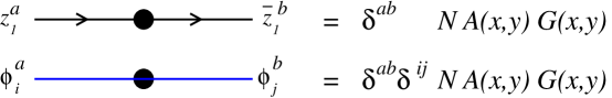
Figure 1: Order $g_{\rm Y\!M}^{2}$ corrections to scalar propagators consist of a gauge boson exchange and a fermion loop.

Feynman rules for the Lagrangian (B.3) are somewhat awkward, but the tree and one-loop diagrams which involve only the scalars can be packaged in a convenient way. First, $\mbox{$\cal O$}(g_{\rm Y\!M}^{2})$ corrections to the scalar propagators are diagonal in color indices, see Figure 1. Fermion loops cancel in $\langle\phi_{2}^{a}(x)\phi_{5}^{b}(y)\rangle_{g_{\rm Y\!M}^{2}}$ because of the way the signs work out in (B).

Corrections to the 4-point irreducible blocks are more involved, but they can be related to the corresponding diagrams involving only $z$-s and $\bar{z}$-s. By comparing two-point functions of the protected operators in the [0,2,0] of $SU(4)$ written on the one hand in terms of $\phi$-fields, and on the other hand in terms of $z$-s and $\bar{z}$-s, we get the diagrams shown in Figure 2. Comparison of two-point functions of the Konishi scalar $\sum_{k=1}^{6}\mbox{tr$\,$}\phi^{k}\phi^{k}=\sum_{k=1}^{3}\mbox{tr$\,$}z^{k}\bar{z}^{k}$ produce the relations listed in Figure 3.

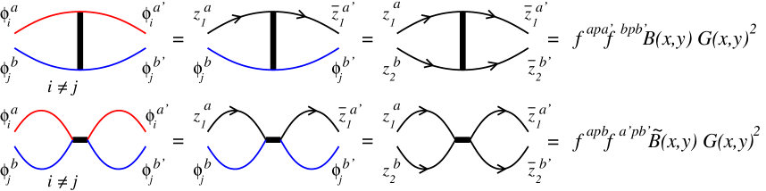
Figure 2: Order $g_{\rm Y\!M}^{2}$ corrections to two point functions of operators of the form $\mbox{tr$\,$}z...\phi^{1}z...\phi^{2}$: four-field irreducible blocks. When scalars $\phi^{i}$ are involved, the diagrams above represent the net contribution of all contributing Feynman diagrams, packaged in a way to mimic the $\cal N$=1 component fields Feynman diagrams. (Thick lines would correspond to exchanges of auxiliary fields $F_{i}$ and $D$ in the $\cal N$=1 formulation.) Diagrams with $z_{2}$ are given for comparison only. There are similar diagrams with one or both $z$-lines running in the opposite direction.

The “$D$-term” contributions $A$ and $B$, and the four-field interaction “$F$-term” $\tilde{B}$ are defined by Figures 2 and 3. As in [27] [16], the $A$ and $B$ are not separately gauge invariant. These must appear as the gauge invariant combination $2A+B$, which vanishes in the $\cal N$=4 theory. So one only has to look at “$F$-term” contributions, which are all proportional to

$$\gamma\equiv\mbox{$1\over 2$}\tilde{B}(x,0)N=-{g_{\rm Y\!M}^{2}N\over 4\pi^{2}}\log x^{2}\mu^{2}\equiv-\beta\log x^{2}\mu^{2}$$ (B.8)

computed for example in [7, 27]. In this paper, we are using the conventions of [7]; in the Lagrangian (B) we have $g_{\rm Y\!M}^{2}=2\pi g$.

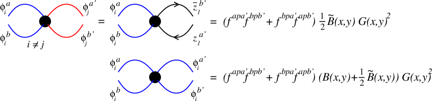
Figure 3: Order $g^{2}$ corrections to two point functions of operators of the form $\mbox{tr$\,$}z...\phi^{1}z...\phi^{1}$: four-field irreducible blocks. Thick lines correspond to exchanges if the gauge boson and auxiliary fields $F_{i}$ and $D$ in the $\cal N$=1 formulation. The diagrams above represent the net contribution of all contributing Feynman diagrams, packaged in a way to mimic the $\cal N$=1 component fields Feynman diagrams.

We only have to consider planar diagrams since we are interested in the leading large $N$ behavior. Put differently,

$$\mbox{tr$\,$}\!\left[t^{a_{1}}...t^{a_{k}}\right]~{}\mbox{tr$\,$}\!\left[t^{a_{k}}...t^{a_{1}}\right]=\left({N\over 2}\right)^{k}\left[1+\mbox{$\cal O$}(1/N^{2})\right]$$ (B.9)

and $SU(N)$ traces of all other permutations of the generators (other than cyclic) are suppressed by $1/N^{2}$. To see this, one can use the “trace merging formula”

$$2\left(\mbox{tr$\,$}At^{c}\right)\left(\mbox{tr$\,$}Bt^{c}\right)=\mbox{tr$\,$}AB-\mbox{$1\over N$}\left(\mbox{tr$\,$}A\right)\left(\mbox{tr$\,$}B\right)$$ (B.10)

valid when $t^{c}$ are $SU(N)$ generators in the fundamental representation.

At one loop, all but the nearest neighbor interactions are suppressed. The relevant contributions in Figure 2 have the form

(B.11)

$$= \mbox{$1\over 2$}\left(\mbox{$1\over 2$}N\right)^{J-1}\mbox{tr$\,$}\left(t^{a}t^{b}t^{b^{\prime}}t^{a^{\prime}}\right)f^{abp}f^{a^{\prime}b^{\prime}p}\left[1+\mbox{$\cal O$}(1/N^{2})\right]$$

$$= \mbox{$1\over 2$}\left(\mbox{$1\over 2$}N\right)^{J-1}\mbox{tr$\,$}\left(t^{a}[t^{p},t^{a}]t^{b^{\prime}}[t^{p},t^{b^{\prime}}]\right)\left[1+\mbox{$\cal O$}(1/N^{2})\right]$$

$$= \left(\mbox{$1\over 2$}N\right)^{J+3}\left[1+\mbox{$\cal O$}(1/N^{2})\right]$$

The difference between the orderings $(ab)$ and $(ba)$ in (B.11) is a minus sign,

$$\mbox{ \begin{picture}(9.5,3.0)\put(0.0,1.5){\line(1,0){9.0}} \put(0.0,-0.5){\line(1,0){9.0}} \put(1.0,1.5){\line(1,-1){2.0}} \put(3.0,1.5){\line(-1,-1){2.0}} \put(5.0,1.5){\line(0,-1){2.0}} \put(8.0,1.5){\line(0,-1){2.0}} \put(5.5,0.0){\makebox(2.0,1.0)[]{...}} \put(1.0,0.0){\makebox(2.0,1.0)[]{\tiny$\bullet$}} \put(0.5,2.0){\makebox(1.0,1.0)[]{$a\phantom{d\!\!\!}$}} \put(0.5,-2.0){\makebox(1.0,1.0)[]{$a^{\prime}\phantom{d\!\!\!}$}} \put(2.5,2.0){\makebox(1.0,1.0)[]{$b\phantom{d\!\!\!}$}} \put(2.5,-2.0){\makebox(1.0,1.0)[]{$b^{\prime}\phantom{d\!\!\!}$}} \put(4.5,2.0){\makebox(1.0,1.0)[]{$c_{1}\phantom{d\!\!\!}$}} \put(4.5,-2.0){\makebox(1.0,1.0)[]{$c_{1}\phantom{d\!\!\!}$}} \put(7.5,2.0){\makebox(1.0,1.0)[]{$c_{J}\phantom{d\!\!\!}$}} \put(7.5,-2.0){\makebox(1.0,1.0)[]{$c_{J}\phantom{d\!\!\!}$}} \end{picture}$\phantom{{}_{\Big{|}}}$}=-\mbox{ \begin{picture}(9.5,3.0)\put(0.0,1.5){\line(1,0){9.0}} \put(0.0,-0.5){\line(1,0){9.0}} \put(1.0,1.5){\line(1,-1){2.0}} \put(3.0,1.5){\line(-1,-1){2.0}} \put(5.0,1.5){\line(0,-1){2.0}} \put(8.0,1.5){\line(0,-1){2.0}} \put(5.5,0.0){\makebox(2.0,1.0)[]{...}} \put(1.0,0.0){\makebox(2.0,1.0)[]{\tiny$\bullet$}} \put(0.5,2.0){\makebox(1.0,1.0)[]{$b\phantom{d\!\!\!}$}} \put(0.5,-2.0){\makebox(1.0,1.0)[]{$a^{\prime}\phantom{d\!\!\!}$}} \put(2.5,2.0){\makebox(1.0,1.0)[]{$a\phantom{d\!\!\!}$}} \put(2.5,-2.0){\makebox(1.0,1.0)[]{$b^{\prime}\phantom{d\!\!\!}$}} \put(4.5,2.0){\makebox(1.0,1.0)[]{$c_{1}\phantom{d\!\!\!}$}} \put(4.5,-2.0){\makebox(1.0,1.0)[]{$c_{1}\phantom{d\!\!\!}$}} \put(7.5,2.0){\makebox(1.0,1.0)[]{$c_{J}\phantom{d\!\!\!}$}} \put(7.5,-2.0){\makebox(1.0,1.0)[]{$c_{J}\phantom{d\!\!\!}$}} \end{picture}$\phantom{{}_{\Big{|}}}$}$$ (B.12)

Diagrams shown in the first two lines of Figure 3 have the form

(B.13)

$$= \mbox{$1\over 2$}\left(\mbox{$1\over 2$}N\right)^{J+3}\left[1+\mbox{$\cal O$}(1/N^{2})\right]$$

Only one of the two $ff$-terms contributes at this order; the other one is suppressed by at least $1/N^{3}$. The contribution (B.13) is insensitive to $a\leftrightarrow b$. The contributions (B.11) and (B.13) come with a numerical prefactor of

$${2\over N}G(x,0)^{J+2}\gamma$$ (B.14)

with $\gamma=-\beta\log x^{2}\mu^{2}$ defined in (B.8).

To summarize, the tree level correlators are

$$\matrix{\psfig{height=79.49744pt}\quad}=(\mbox{$1\over 2$}GN)^{J+{\mathsf{N}}}$$ (B.15)

and the relevant one-loop contributions can be schematically represented as

$$\matrix{\psfig{height=50.58878pt}}=-\matrix{\psfig{height=50.58878pt}} = \gamma\times(\mbox{$1\over 2$}GN)^{J+{\mathsf{N}}}$$ (B.16)

when only one $\phi$ is involved in the interaction, and

$$\matrix{\psfig{height=50.58878pt}}=-\matrix{\psfig{height=50.58878pt}} = \gamma\times(\mbox{$1\over 2$}GN)^{J+{\mathsf{N}}},\quad i\neq j$$ (B.17)

when two distinct $\phi$ within either trace interact. Furthermore, we have

$$\matrix{\psfig{height=50.58878pt}}=\matrix{\psfig{height=50.58878pt}}=\matrix{\psfig{height=50.58878pt}} = {1\over 2}\,\gamma\times(\mbox{$1\over 2$}GN)^{J+{\mathsf{N}}},\quad i\neq j$$

Finally, the diagrams which involve a $zz\bar{z}\bar{z}$ vertex can be read off from (B.17) and (B) by expanding the $z$ and $\bar{z}$ participating in the vertex in terms of the two remaining $\phi$’s,

$$\matrix{\psfig{height=50.58878pt}}=-{1\over 2}\,\gamma\times(\mbox{$1\over 2$}GN)^{J+{\mathsf{N}}},\hskip 20.00003pt\matrix{\psfig{height=50.58878pt}} = {3\over 2}\,\gamma\times(\mbox{$1\over 2$}GN)^{J+{\mathsf{N}}}$$

In the results (B.15)-(B), we dropped terms suppressed by $1/N^{2}$.

Appendix C Equality of matrix elements: generic states

In this appendix we will complete matching the matrix elements of the light cone Hamiltonian between the two sides of the AdS/CFT correspondence. In section 3.3 we matched matrix elements for a subset of states. There we considered states with all excited modes having distinct SO(4) indices $i_{k}$, and no mode excited more than once. We will now consider states with some $i_{k}$ being equal. We initially restrict to the case with no modes excited more than once, $N^{i}_{n}\leq 1$, but will eventually generalize to most general case.

In contrast with section 3.3, ${\cal O}_{*}$ no longer vanishes. In addition to (3.33), we now have to consider off-diagonal elements between the states

$$|{\cal Y}\rangle=y_{n_{1}}^{i_{1}}{}^{\dagger}\ldots y_{m}^{i}{}^{\dagger}y_{n}^{i}{}^{\dagger}|\eta\rangle,\qquad m\neq n,$$ (C.1)

and

$$|{\cal Y}^{\prime}\rangle=y_{n_{1}}^{i_{1}}{}^{\dagger}\ldots y_{m}^{j}{}^{\dagger}y_{n}^{j}{}^{\dagger}|\eta\rangle,\qquad m\neq n,$$ (C.2)

which are given by

$$\langle{\cal Y}|H_{1}^{OD}|{\cal Y}^{\prime}\rangle={1\over J}\left({R^{2}\over J}\right)^{2}mn\sqrt{N^{i}_{m}N^{i}_{n}N^{j}_{m}{}^{\prime}N^{j}_{n}{}^{\prime}}.$$ (C.3)

There is also an off-diagonal element given by (3.33), but we have analyzed all diagrams contributing to it in section 3.3. Let us briefly explain why this is the case. Consider ${\cal O}(g^{0})$ part of the contributing two-point function, which we denote by $\langle{\cal X}{\bar{\cal X}}^{\prime}\rangle_{g^{0}}$. $\langle{\tilde{\cal X}}{\bar{\cal X}}_{*}^{\prime}\rangle_{g^{0}}$ and $\langle{\cal X}_{*}^{\prime}{\bar{\tilde{\cal X}}}\rangle_{g^{0}}$ vanish, as there are no contributing interaction-free diagrams. Although $\langle{\cal X}_{*}{\bar{\cal X}^{\prime}}_{*}\rangle_{g^{0}}$ has nonvanishing terms, they are ${\cal O}(1/J^{2})$. This is because ${\cal X}_{*}$ is itself ${\cal O}(1/J)$ compared to ${\tilde{\cal O}}$, and an additional factor of $1/J$ will appear because phases in ${\cal X}_{*}$ and ${\cal X}_{*}^{\prime}$ do not match exactly. Similar conclusions can be made about ${\cal O}(g)$ correlator $\langle{\tilde{\cal X}}{\bar{\cal X}^{\prime}}\rangle_{g^{1}}$.

Let us compute the off-diagonal element (C.3) in the gauge theory. The only contribution to $\langle{\cal Y}(x){\bar{\cal Y}^{\prime}}(0)\rangle_{g^{0}}$ comes from

$$\langle{\cal Y}_{*}(x){\bar{\cal Y}^{\prime}}_{*}(0)\rangle_{g^{0}}={1\over\Omega}\sum\mbox{ \begin{picture}(9.5,3.0)\put(0.0,1.5){\line(1,0){9.0}} \put(0.0,-0.5){\line(1,0){9.0}} \put(1.0,1.5){\line(0,-1){2.0}} \put(4.5,1.5){\line(0,-1){2.0}} \put(8.0,1.5){\line(0,-1){2.0}} \put(5.0,0.0){\makebox(2.0,1.0)[]{...}} \put(1.5,0.0){\makebox(2.0,1.0)[]{...}} \put(0.5,2.0){\makebox(1.0,1.0)[]{${\check{\phi}}^{i}_{m}\phantom{d\!\!\!}$}} \put(0.5,-2.0){\makebox(1.0,1.0)[]{${\check{\phi}}^{j}_{m}\phantom{d\!\!\!}$}} \put(4.0,2.0){\makebox(1.0,1.0)[]{${\check{\phi}}^{i}_{n}\phantom{d\!\!\!}$}} \put(4.0,-2.0){\makebox(1.0,1.0)[]{${\check{\phi}}^{j}_{n}\phantom{d\!\!\!}$}} \put(7.5,2.0){\makebox(1.0,1.0)[]{$\phi^{i_{k}}_{n_{k}}\phantom{d\!\!\!}$}} \put(7.5,-2.0){\makebox(1.0,1.0)[]{$\phi^{i_{k}}_{n_{k}}\phantom{d\!\!\!}$}} \end{picture}$\phantom{{}_{\Big{|}}}$}={1\over J},$$ (C.4)

where the sum runs over all configurations of fields. No ${\cal O}(g^{0})$ diagrams appear in $\langle{\tilde{\cal Y}}{\bar{\cal Y}^{\prime}}_{*}\rangle_{g^{0}}$, $\langle{\cal Y}_{*}{\bar{\tilde{\cal Y}^{\prime}}}\rangle_{g^{0}}$ and $\langle{\tilde{\cal Y}}{\bar{\tilde{\cal Y}^{\prime}}}\rangle_{g^{0}}$. Hence we have

$${\bf T}^{(1)}_{{\cal Y}{\cal Y}^{\prime}}=1.$$ (C.5)

Computation of ${\bf F}_{{\cal Y}{\cal Y}^{\prime}}$ is more involved. Possible contributions are

$$\langle{\tilde{\cal Y}}(x){\bar{\tilde{\cal Y}^{\prime}}}(0)\rangle_{g^{1}} = {1\over\Omega}{\sum}{\mbox{ \begin{picture}(9.5,3.0)\put(0.0,1.5){\line(1,0){9.0}} \put(0.0,-0.5){\line(1,0){9.0}} \put(1.0,1.5){\line(1,-1){2.0}} \put(3.0,1.5){\line(-1,-1){2.0}} \put(5.0,1.5){\line(0,-1){2.0}} \put(8.0,1.5){\line(0,-1){2.0}} \put(5.5,0.0){\makebox(2.0,1.0)[]{...}} \put(1.0,0.0){\makebox(2.0,1.0)[]{\tiny$\bullet$}} \put(0.5,2.0){\makebox(1.0,1.0)[]{$\phi^{i}_{m}\phantom{d\!\!\!}$}} \put(0.5,-2.0){\makebox(1.0,1.0)[]{$\phi^{j}_{m^{\prime}}\phantom{d\!\!\!}$}} \put(2.5,2.0){\makebox(1.0,1.0)[]{$\phi^{i}_{n}\phantom{d\!\!\!}$}} \put(2.5,-2.0){\makebox(1.0,1.0)[]{$\phi^{j}_{n^{\prime}}\phantom{d\!\!\!}$}} \put(4.5,2.0){\makebox(1.0,1.0)[]{$z\phantom{d\!\!\!}$}} \put(4.5,-2.0){\makebox(1.0,1.0)[]{$\bar{z}\phantom{d\!\!\!}$}} \put(7.5,2.0){\makebox(1.0,1.0)[]{$\phi^{i_{k}}_{n_{k}}\phantom{d\!\!\!}$}} \put(7.5,-2.0){\makebox(1.0,1.0)[]{$\phi^{i_{k}}_{n_{k}}\phantom{d\!\!\!}$}} \end{picture}$\phantom{{}_{\Big{|}}}$}}{+}(m{\leftrightarrow}n){+}(m^{\prime}{\leftrightarrow}n^{\prime}){+}(m{\leftrightarrow}n,m^{\prime}{\leftrightarrow}n^{\prime})$$

$$= {\gamma\over 2J}(q_{n-m}+q_{n-m}^{*}+2),$$

which holds both for $m^{\prime}=n,n^{\prime}=m$ (off-diagonal) and $m^{\prime}=m,n^{\prime}=n$ (diagonal),

$${-}\langle{\tilde{\cal Y}}(x){\bar{\cal Y}^{\prime}}_{*}(0)\rangle_{g^{1}} = {-}{1\over\Omega}{\sum}\mbox{ \begin{picture}(9.5,3.0)\put(0.0,1.5){\line(1,0){9.0}} \put(0.0,-0.5){\line(1,0){9.0}} \put(1.0,1.5){\line(1,-1){2.0}} \put(3.0,1.5){\line(-1,-1){2.0}} \put(5.0,1.5){\line(0,-1){2.0}} \put(8.0,1.5){\line(0,-1){2.0}} \put(5.5,0.0){\makebox(2.0,1.0)[]{...}} \put(1.0,0.0){\makebox(2.0,1.0)[]{\tiny$\bullet$}} \put(0.5,2.0){\makebox(1.0,1.0)[]{$\phi^{i}_{m}\phantom{d\!\!\!}$}} \put(0.5,-2.0){\makebox(1.0,1.0)[]{$z\phantom{d\!\!\!}$}} \put(2.5,2.0){\makebox(1.0,1.0)[]{$\phi^{i}_{n}\phantom{d\!\!\!}$}} \put(2.5,-2.0){\makebox(1.0,1.0)[]{$\bar{z}\phantom{d\!\!\!}$}} \put(4.5,2.0){\makebox(1.0,1.0)[]{$z\phantom{d\!\!\!}$}} \put(4.5,-2.0){\makebox(1.0,1.0)[]{$\bar{z}\phantom{d\!\!\!}$}} \put(7.5,2.0){\makebox(1.0,1.0)[]{$\phi^{i_{k}}_{n_{k}}\phantom{d\!\!\!}$}} \put(7.5,-2.0){\makebox(1.0,1.0)[]{$\phi^{i_{k}}_{n_{k}}\phantom{d\!\!\!}$}} \end{picture}$\phantom{{}_{\Big{|}}}$}{+}(m{\leftrightarrow}n){+}(z{\leftrightarrow}{\bar{z}}){+}(m{\leftrightarrow}n,z{\leftrightarrow}{\bar{z}})$$

$$= -{\gamma\over 2J}(q_{m}+q_{m}^{*}+q_{n}+q_{n}^{*}),$$

similar contribution from $\langle{\cal Y}_{*}(x){\bar{\cal Y}^{\prime}}_{*}(0)\rangle_{g^{1}}$, and

$$\langle{\cal Y}_{*}(x){\bar{\cal Y}^{\prime}}_{*}(0)\rangle_{g^{1}}={1\over\Omega}{\sum}\mbox{ \begin{picture}(9.5,3.0)\put(0.0,1.5){\line(1,0){9.0}} \put(0.0,-0.5){\line(1,0){9.0}} \put(1.0,1.5){\line(0,-1){2.0}} \put(3.0,1.5){\line(0,-1){2.0}} \put(6.0,1.5){\line(1,-1){2.0}} \put(8.0,1.5){\line(-1,-1){2.0}} \put(4.0,0.0){\makebox(2.0,1.0)[]{...}} \put(1.0,0.0){\makebox(12.0,1.0)[]{\tiny$\bullet$}} \put(0.5,2.0){\makebox(1.0,1.0)[]{$z\phantom{d\!\!\!}$}} \put(0.5,-2.0){\makebox(1.0,1.0)[]{$\bar{z}\phantom{d\!\!\!}$}} \put(2.5,2.0){\makebox(1.0,1.0)[]{$\;\;\bar{z}_{m{+}n}\phantom{d\!\!\!}$}} \put(2.5,-2.0){\makebox(1.0,1.0)[]{$\;\;z_{m{+}n}\phantom{d\!\!\!}$}} \put(5.5,2.0){\makebox(1.0,1.0)[]{$\phi^{i_{k}}_{n_{k}}\phantom{d\!\!\!}$}} \put(5.5,-2.0){\makebox(1.0,1.0)[]{$\bar{z}\phantom{d\!\!\!}$}} \put(7.5,2.0){\makebox(1.0,1.0)[]{$z\phantom{d\!\!\!}$}} \put(7.5,-2.0){\makebox(1.0,1.0)[]{$\phi^{i_{k}}_{n_{k}}\phantom{d\!\!\!}$}} \end{picture}$\phantom{{}_{\Big{|}}}$}{+}(\phi^{i_{k}}_{n_{k}}{\leftrightarrow}z){+}(\phi^{i_{k}}_{n_{k}}{\leftrightarrow}{\bar{z}})$$ (C.8)

$$\qquad\qquad\qquad\qquad\qquad\qquad\qquad\qquad\qquad{+}(\phi^{i_{k}}_{n_{k}}{\leftrightarrow}z,\phi^{i_{k}}_{n_{k}}{\leftrightarrow}{\bar{z}})$$

$$\qquad\qquad{+}{1\over\Omega}\sum\mbox{ \begin{picture}(9.5,3.0)\put(0.0,1.5){\line(1,0){9.0}} \put(0.0,-0.5){\line(1,0){9.0}} \put(1.0,1.5){\line(1,-1){2.0}} \put(3.0,1.5){\line(-1,-1){2.0}} \put(5.0,1.5){\line(0,-1){2.0}} \put(8.0,1.5){\line(0,-1){2.0}} \put(5.5,0.0){\makebox(2.0,1.0)[]{...}} \put(1.0,0.0){\makebox(2.0,1.0)[]{\tiny$\bullet$}} \put(0.5,2.0){\makebox(1.0,1.0)[]{$z\phantom{d\!\!\!}$}} \put(0.5,-2.0){\makebox(1.0,1.0)[]{$\bar{z}\phantom{d\!\!\!}$}} \put(2.5,2.0){\makebox(1.0,1.0)[]{$\bar{z}_{m{+}n}\phantom{d\!\!\!}$}} \put(2.5,-2.0){\makebox(1.0,1.0)[]{$z_{m{+}n}\phantom{d\!\!\!}$}} \put(4.5,2.0){\makebox(1.0,1.0)[]{$z\phantom{d\!\!\!}$}} \put(4.5,-2.0){\makebox(1.0,1.0)[]{$\bar{z}\phantom{d\!\!\!}$}} \put(7.5,2.0){\makebox(1.0,1.0)[]{$\phi^{i_{k}}_{n_{k}}\phantom{d\!\!\!}$}} \put(7.5,-2.0){\makebox(1.0,1.0)[]{$\phi^{i_{k}}_{n_{k}}\phantom{d\!\!\!}$}} \end{picture}$\phantom{{}_{\Big{|}}}$}{+}(z{\leftrightarrow}{\bar{z}_{m{+}n}}){+}({\bar{z}}\leftrightarrow z_{m{+}n}){+}(z{\leftrightarrow}{\bar{z}_{m{+}n}},{\bar{z}}\leftrightarrow z_{m{+}n})$$

$$\qquad={\gamma\over J}\left(-\sum_{p:\,n_{p}\neq m,n}(q_{n_{p}}+q_{n_{p}}^{*}-2)-{1\over 2}(q_{m+n}+q_{m+n}^{*})+3\right).$$

(Recall that the subscript in ${\bar{z}}_{n+m}$ stands for the phase $q_{n+m}^{a_{\bar{z}}}$ which depends on the position of the $\bar{z}$ in the string of operators.) Combining (C.5)–(C.8) we have

$$[{\bf T}^{-1}{\bf F}]_{{\cal Y}{\cal Y}^{\prime}}=-{\beta\over 2J}(q_{m+n}-q_{m-n}+c.c.)={1\over J}\left({R^{2}\over J}\right)^{2}mn,$$ (C.9)

which indeed agrees with (C.3), provided $N^{i}_{n}\leq 1$.

Let us now turn to the diagonal matrix element. Part of it was computed in section 3.3 and is given by (3.57). But now there are other contributions both to ${\bf T}^{(1)}_{{\cal O}{\cal O}}$ and to ${\bf F}_{{\cal O}{\cal O}}$. To update the former, we must take into account

$$\langle{\cal O}_{*}(x){\bar{\cal O}}_{*}(0)\rangle_{g^{0}}={1\over\Omega}\sum_{i,(m\neq n)}\sum\mbox{ \begin{picture}(9.5,3.0)\put(0.0,1.5){\line(1,0){9.0}} \put(0.0,-0.5){\line(1,0){9.0}} \put(1.0,1.5){\line(0,-1){2.0}} \put(4.5,1.5){\line(0,-1){2.0}} \put(8.0,1.5){\line(0,-1){2.0}} \put(5.0,0.0){\makebox(2.0,1.0)[]{...}} \put(1.5,0.0){\makebox(2.0,1.0)[]{...}} \put(0.5,2.0){\makebox(1.0,1.0)[]{${\check{\phi}}^{i}_{m}\phantom{d\!\!\!}$}} \put(0.5,-2.0){\makebox(1.0,1.0)[]{${\check{\phi}}^{i}_{m}\phantom{d\!\!\!}$}} \put(4.0,2.0){\makebox(1.0,1.0)[]{${\check{\phi}}^{i}_{n}\phantom{d\!\!\!}$}} \put(4.0,-2.0){\makebox(1.0,1.0)[]{${\check{\phi}}^{i}_{n}\phantom{d\!\!\!}$}} \put(7.5,2.0){\makebox(1.0,1.0)[]{$\phi^{i_{k}}_{n_{k}}\phantom{d\!\!\!}$}} \put(7.5,-2.0){\makebox(1.0,1.0)[]{$\phi^{i_{k}}_{n_{k}}\phantom{d\!\!\!}$}} \end{picture}$\phantom{{}_{\Big{|}}}$}=\sum_{i}{{\mathsf{N}}_{i}({\mathsf{N}}_{i}-1)\over 2J},$$ (C.10)

and

$$\delta\langle{\tilde{\cal O}}(x){\bar{\tilde{\cal O}}}(0)\rangle_{g^{0}}={1\over\Omega}\sum_{i,(m\neq n)}\sum\mbox{ \begin{picture}(9.5,3.0)\put(0.0,1.5){\line(1,0){9.0}} \put(0.0,-0.5){\line(1,0){9.0}} \put(1.0,1.5){\line(0,-1){2.0}} \put(4.5,1.5){\line(0,-1){2.0}} \put(8.0,1.5){\line(0,-1){2.0}} \put(5.0,0.0){\makebox(2.0,1.0)[]{...}} \put(1.5,0.0){\makebox(2.0,1.0)[]{...}} \put(0.5,2.0){\makebox(1.0,1.0)[]{$\phi^{i}_{m}\phantom{d\!\!\!}$}} \put(0.5,-2.0){\makebox(1.0,1.0)[]{$\phi^{i}_{n}\phantom{d\!\!\!}$}} \put(4.0,2.0){\makebox(1.0,1.0)[]{$\phi^{i}_{n}\phantom{d\!\!\!}$}} \put(4.0,-2.0){\makebox(1.0,1.0)[]{$\phi^{i}_{m}\phantom{d\!\!\!}$}} \put(7.5,2.0){\makebox(1.0,1.0)[]{$\phi^{i_{k}}_{n_{k}}\phantom{d\!\!\!}$}} \put(7.5,-2.0){\makebox(1.0,1.0)[]{$\phi^{i_{k}}_{n_{k}}\phantom{d\!\!\!}$}} \end{picture}$\phantom{{}_{\Big{|}}}$}=-\sum_{i}{{\mathsf{N}}_{i}({\mathsf{N}}_{i}-1)\over 2J},$$ (C.11)

which cancels (C.10) to keep ${\bf T}_{{\cal O}{\cal O}}=1$. The ${\cal O}(g^{1})$ correlators related to (C.10) are given by the sum of (C.8) over pairs $(n_{k}\neq n_{l}):i_{k}=i_{l}$ with the substitution $m=n_{k},n=n_{l}$:

$$\langle{\cal O}_{*}(x){\bar{\cal O}}_{*}(0)\rangle_{g^{1}} = {\gamma\over J}\sum_{(n_{k}{\neq}n_{l}):i_{k}{=}i_{l}}\left(3{-}\sum_{p{\neq}k,l}(q_{n_{p}}{+}q_{n_{p}}^{*}{-}2)-{1\over 2}(q_{n_{k}{+}n_{l}}{+}q_{n_{k}{+}n_{l}}^{*})\right)$$

$$= {\gamma\over J}\Bigg{[}-\left(\sum_{i}{{\mathsf{N}}_{i}({\mathsf{N}}_{i}{-}1)\over 2}\right)\sum_{k}(q_{n_{k}}{+}q_{n_{k}}^{*}{-}2)$$

$$\quad+\sum_{(n_{k}{\neq}n_{l}):i_{k}=i_{l}}\left\{(q_{n_{k}}+q_{n_{l}}-2+c.c.)-{1\over 2}(q_{n_{k}+n_{l}}+q_{n_{k}+n_{l}}^{*})+3\right\}\Bigg{]}.$$

The ${\cal O}(g^{1})$ counterpart of (C.11) is

$$\delta_{1}\langle{\tilde{\cal O}}(x){\bar{\tilde{\cal O}}}(0)\rangle_{g^{1}}{=}{\gamma\over J}\bigg{[}\left(\sum_{i}{{\mathsf{N}}_{i}({\mathsf{N}}_{i}{-}1)\over 2}\right)\sum_{k}(q_{n_{k}}{+}q_{n_{k}}^{*}{-}2)+\!\!\sum_{(n_{k}{\neq}n_{l}):i_{k}{=}i_{l}}\!\!(q_{n_{k}}{+}q_{n_{l}}{-}2q_{n_{l}{-}n_{k}}{+}c.c.)\bigg{]}.$$ (C.13)

The first term in this expression is a value of the corresponding interaction-free diagram times the sum of possible phases, while the second term takes care of overcounted corrections (this technique for computing ${\cal O}(g^{1})$ diagrams was explained in more detail in section 3.3) There is also a contribution which is a direct analog of (3.55)

$$\delta_{2}\langle{\tilde{\cal O}}(x){\bar{\tilde{\cal O}}}(0)\rangle_{g^{1}}{=}{\gamma\over J}\sum_{(n_{k}{\neq}n_{l}):i_{k}{=}i_{l}}\left[(q_{n_{k}}+q_{n_{l}}-2+c.c.)+{1\over 2}(q_{n_{k}-n_{l}}+q_{n_{k}-n_{l}}^{*}+2)\right].$$ (C.14)

Finally, we should include the sum over pairs in (C) and the same term due to

$$-\langle{\cal Y}_{*}(x){\bar{\tilde{\cal Y}^{\prime}}}(0){+}{\tilde{\cal Y}}(x){\bar{\cal Y}^{\prime}}_{*}(0)\rangle_{g^{1}}=-{\gamma\over J}\sum_{(n_{k}{\neq}n_{l}):i_{k}{=}i_{l}}(q_{n_{k}}+q_{n_{l}}+c.c.),$$ (C.15)

Combining (C)–(C.15) we get

$$\delta[{\bf T}^{-1}{\bf F}]_{{\cal O}{\cal O}} = -{\beta\over 2J}\sum_{(n_{k}{\neq}n_{l}):i_{k}{=}i_{l}}\left[3q_{n_{k}{-}n_{l}}{+}q_{n_{k}{+}n_{l}}{-}4q_{n_{k}}{-}4q_{n_{l}}{+}4{+}c.c.\right]$$

$$= {-}{1\over J}\left({R^{2}\over J}\right)^{2}\sum_{(n_{k}{\neq}n_{l}):i_{k}{=}i_{l}}n_{k}n_{l},$$

which should be added to (3.57). In the case of $N^{i}_{m}\leq 1$, (C) combined with the last term in (3.57) gives

$$-{1\over J}\left({R^{2}\over J}\right)^{2}\left[\sum_{(k,l):i_{k}{\neq}i_{l}}n_{k}n_{l}+\sum_{(n_{k}{\neq}n_{l}):i_{k}{=}i_{l}}n_{k}n_{l}\right]={1\over 2J}\left({R^{2}\over J}\right)^{2}\sum_{k}n_{k}^{2},$$ (C.17)

where we used the level matching condition. Hence we again reproduce (3.35).

Our last step will be generalization to the case of unconstrained $N^{i}_{n}$. To see how (3.54) is modified recall that all contributing correlators should be divided by

$$\sqrt{N^{i}_{m}!N^{j}_{n}!N^{i}_{n}!N^{j}_{m}!N^{i}_{m}{}^{\prime}!N^{j}_{n}{}^{\prime}!N^{i}_{n}{}^{\prime}!N^{j}_{m}{}^{\prime}!\ldots}$$ (C.18)

where $\ldots$ stands for other $N^{i_{k}}_{n_{k}}$ which will be cancelled by the number of possible contractions, just as they are cancelled in non-interacting diagrams to produce $T_{{\cal O}{\cal O}}=1+{\cal O}(1/J)$. On the other hand, the combinatorial factor that multiplies all the correlators contributing to (3.54) is

$$N^{i}_{m}!N^{j}_{n}!N^{i}_{n}{}^{\prime}!N^{j}_{m}{}^{\prime}!\ldots$$ (C.19)

The ratio of (C.19) and (C.18) is precisely the factor $\sqrt{N^{i}_{m}N^{j}_{n}N^{i}_{n}{}^{\prime}N^{j}_{m}{}^{\prime}}$ which appears in (3.54). The combinatorial factor in (C.3) can be restored in the similar manner.

In addition to (3.33) and (C.3) we also need to consider off-diagonal matrix elements between the states

$$|{\cal Z}\rangle=y_{n_{1}}^{i_{1}}{}^{\dagger}\ldots y_{n}^{i}{}^{\dagger}y_{n}^{i}{}^{\dagger}|\eta\rangle,$$ (C.20)

and

$$|{\cal Z}^{\prime}\rangle=y_{n_{1}}^{i_{1}}{}^{\dagger}\ldots y_{n}^{j}{}^{\dagger}y_{n}^{j}{}^{\dagger}|\eta\rangle,$$ (C.21)

which are given by

$$\langle{\cal Z}|H_{1}^{OD}|{\cal Z}^{\prime}\rangle={1\over 4J}\left({R^{2}\over J}\right)^{2}n^{2}\sqrt{N^{i}_{n}(N^{i}_{n}-1)N^{j}_{n}{}^{\prime}(N^{j}_{n}{}^{\prime}-1)}.$$ (C.22)

This can be computed similarly to (C.9). One should just multiply each term in (C.5)–(C.8) by

$${J^{\mathsf{N}}\over\sqrt{{\tilde{\Omega}}\,{\tilde{\Omega}}^{\prime}}}{N^{i}_{n}(N^{i}_{n}-1)\over 2}{N^{j}_{n}{}^{\prime}(N^{j}_{n}{}^{\prime}-1)\over 2}(N^{i}_{n}-2)!\,(N^{j}_{n}{}^{\prime}-2)!.$$ (C.23)

The ingredients in (C.23) correspond to the normalization, the number of possible choices of a pair out of $N^{i}_{n}$ ($N^{j}_{n}{}^{\prime}$) $\phi^{i}_{n}$’s ( $\phi^{j}_{n}$’s), and the number of permutations of the leftover $\phi^{i}_{n}$’s ( $\phi^{j}_{n}$’s). Substituting ${\tilde{\Omega}}\approx\sqrt{J^{\mathsf{N}}N^{i}_{n}!N^{j}_{n}!\ldots}$ and ${\tilde{\Omega}}^{\prime}\approx\sqrt{J^{\mathsf{N}}N^{i}_{n}{}^{\prime}!N^{j}_{n}{}^{\prime}!\ldots}$ into (C.23) one recovers correct combinatorial factor in (C.22).

The expressions for diagonal matrix elements (3.57) and (C) do not change when we allow $N^{i}_{n}>1$. However (C.17) changes to

$${1\over 2J}\left({R^{2}\over J}\right)^{2}\sum_{i,n}n^{2}(N^{i}_{n})^{2}.$$ (C.24)

There is an additional contribution to the diagonal matrix element, which is similar to (C) but with $n_{l}=n_{k}$. To compute it, one has to follow the logic which led to (C) paying special attention to combinatorial factors. We now have

$$\delta\langle{\cal O}_{*}(x){\bar{\cal O}}_{*}(0)\rangle_{g^{0}}={1\over\Omega}\sum_{i,n}\sum\mbox{ \begin{picture}(9.5,3.0)\put(0.0,1.5){\line(1,0){9.0}} \put(0.0,-0.5){\line(1,0){9.0}} \put(1.0,1.5){\line(0,-1){2.0}} \put(4.5,1.5){\line(0,-1){2.0}} \put(8.0,1.5){\line(0,-1){2.0}} \put(5.0,0.0){\makebox(2.0,1.0)[]{...}} \put(1.5,0.0){\makebox(2.0,1.0)[]{...}} \put(0.5,2.0){\makebox(1.0,1.0)[]{${\check{\phi}}^{i}_{n}\phantom{d\!\!\!}$}} \put(0.5,-2.0){\makebox(1.0,1.0)[]{${\check{\phi}}^{i}_{n}\phantom{d\!\!\!}$}} \put(4.0,2.0){\makebox(1.0,1.0)[]{${\check{\phi}}^{i}_{n}\phantom{d\!\!\!}$}} \put(4.0,-2.0){\makebox(1.0,1.0)[]{${\check{\phi}}^{i}_{n}\phantom{d\!\!\!}$}} \put(7.5,2.0){\makebox(1.0,1.0)[]{$\phi^{i_{k}}_{n_{k}}\phantom{d\!\!\!}$}} \put(7.5,-2.0){\makebox(1.0,1.0)[]{$\phi^{i_{k}}_{n_{k}}\phantom{d\!\!\!}$}} \end{picture}$\phantom{{}_{\Big{|}}}$}=\sum_{i,n}{N^{i}_{n}(N^{i}_{n}-1)\over 4J}$$ (C.25)

and

$$\delta\langle{\tilde{\cal O}}(x){\bar{\tilde{\cal O}}}(0)\rangle_{g^{0}}=0.$$ (C.26)

since the diagram analogous to (C.10) with $m=n$ have been already taken care of, and absorbed in the normalization constant. The analog of (C) is

$$\delta\langle{\cal O}_{*}(x){\bar{\cal O}}_{*}(0)\rangle_{g^{1}}{=}{\gamma\over J}\sum_{i,n}{N^{i}_{n}(N^{i}_{n}{-}1)\over 4}\bigg{[}-\sum_{k}(q_{n_{k}}{+}q_{n_{k}}^{*}{-}2){+}2(q_{n}{+}q_{n}^{*}{-}2){-}{1\over 2}(q_{2n}+q_{2n}^{*}){+}3\bigg{]},$$ (C.27)

while the contribution similar to (C.13) is absent. The analog of (C.14) is

$$\delta_{3}\langle{\tilde{\cal O}}(x){\bar{\tilde{\cal O}}}(0)\rangle_{g^{1}}{=}{\gamma\over J}\sum_{i,n}{N^{i}_{n}(N^{i}_{n}-1)\over 4}\left[4(q_{n}+q_{n}^{*}-2)+2\right].$$ (C.28)

Finally, there is an analog of (C.15) given by

$$-\delta\langle{\cal O}_{*}(x){\bar{\tilde{\cal O}^{\prime}}}(0){+}{\tilde{\cal O}}(x){\bar{\cal O}}_{*}(0)\rangle_{g^{1}}=-{\gamma\over J}\sum_{i,n}{N^{i}_{n}(N^{i}_{n}-1)\over 2}(q_{n}+q_{n}^{*}).$$ (C.29)

Combining (C.25)–(C.29) we get the following contribution to the diagonal matrix element from the $\phi^{i}_{n}/\phi^{i}_{n}$ interactions

$${\beta\over J}\sum_{i,n}{N^{i}_{n}(N^{i}_{n}-1)\over 4}\left(4q_{n}-{q_{2n}\over 2}+c.c.\right)=-{1\over J}\left({R^{2}\over J}\right)^{2}\sum_{i,n}{n^{2}N^{i}_{n}(N^{i}_{n}-1)\over 4}.$$ (C.30)

Adding this to (C.24) and then replacing the last term in (3.57) with the resulting expression we recover the string theory result (3.35). This concludes the matching of matrix elements between the string and the gauge theory.

References

• [1] J. M. Maldacena, “The large $N$ limit of superconformal field theories and supergravity,” Adv. Theor. Math. Phys.  2, 231 (1998) [Int. J. Theor. Phys.  38, 1113 (1999)] [arXiv:hep-th/9711200].
• [2] S. S. Gubser, I. R. Klebanov and A. M. Polyakov, “Gauge theory correlators from non-critical string theory,” Phys. Lett. B 428, 105 (1998) [arXiv:hep-th/9802109].
• [3] E. Witten, “Anti-de Sitter space and holography,” Adv. Theor. Math. Phys.  2, 253 (1998) [arXiv:hep-th/9802150].
• [4] A complete list of credits would take many pages. See for example the reviews O. Aharony, S. S. Gubser, J. M. Maldacena, H. Ooguri and Y. Oz, “Large N field theories, string theory and gravity,” Phys. Rept.  323, 183 (2000) [arXiv:hep-th/9905111]. E. D’Hoker and D. Z. Freedman, “Supersymmetric gauge theories and the AdS/CFT correspondence,” arXiv:hep-th/0201253. and references therein.
• [5] R. R. Metsaev, “Type IIB Green-Schwarz superstring in plane wave Ramond-Ramond background,” Nucl. Phys. B 625, 70 (2002) [arXiv:hep-th/0112044].
• [6] R. R. Metsaev and A. A. Tseytlin, “Exactly solvable model of superstring in plane wave Ramond-Ramond background,” Phys. Rev. D 65, 126004 (2002) [arXiv:hep-th/0202109].
• [7] D. Berenstein, J. M. Maldacena and H. Nastase, “Strings in flat space and pp waves from N = 4 super Yang Mills,” JHEP 0204, 013 (2002) [arXiv:hep-th/0202021].
• [8] M. Blau, J. Figueroa-O’Farrill, C. Hull and G. Papadopoulos, “Penrose limits and maximal supersymmetry,” Class. Quant. Grav.  19, L87 (2002) [arXiv:hep-th/0201081].
• [9] D. J. Gross, A. Mikhailov and R. Roiban, “Operators with large R charge in N = 4 Yang-Mills theory,” arXiv:hep-th/0205066.
• [10] A. Santambrogio and D. Zanon, “Exact anomalous dimensions of N = 4 Yang-Mills operators with large R charge,” arXiv:hep-th/0206079.
• [11] C. Kristjansen, J. Plefka, G. W. Semenoff and M. Staudacher, “A new double-scaling limit of N = 4 super Yang-Mills theory and PP-wave strings,” arXiv:hep-th/0205033.
• [12] M. Spradlin and A. Volovich, “Superstring interactions in a pp-wave background,” arXiv:hep-th/0204146.
• [13] M. Spradlin and A. Volovich, “Superstring interactions in a pp-wave background. II,” arXiv:hep-th/0206073.
• [14] I. R. Klebanov, M. Spradlin and A. Volovich, “New effects in gauge theory from pp-wave superstrings,” arXiv:hep-th/0206221.
• [15] D. Berenstein and H. Nastase, “On lightcone string field theory from super Yang-Mills and holography,” arXiv:hep-th/0205048.
• [16] N. R. Constable, D. Z. Freedman, M. Headrick, S. Minwalla, L. Motl, A. Postnikov and W. Skiba, “PP-wave string interactions from perturbative Yang-Mills theory,” JHEP 0207, 017 (2002) [arXiv:hep-th/0205089].
• [17] Y. j. Kiem, Y. b. Kim, S. m. Lee and J. m. Park, “pp-wave / Yang-Mills correspondence: An explicit check,” arXiv:hep-th/0205279.
• [18] M. x. Huang, “Three point functions of N = 4 super Yang Mills from light cone string field theory in pp-wave,” arXiv:hep-th/0205311; M. x. Huang, “String interactions in pp-wave from N = 4 super Yang Mills,” arXiv:hep-th/0206248.
• [19] C. S. Chu, V. V. Khoze and G. Travaglini, “Three-point functions in N = 4 Yang-Mills theory and pp-waves,” JHEP 0206, 011 (2002) [arXiv:hep-th/0206005]; C. S. Chu, V. V. Khoze and G. Travaglini, arXiv:hep-th/0206167.
• [20] P. Lee, S. Moriyama and J. w. Park, “Cubic interactions in pp-wave light cone string field theory,” arXiv:hep-th/0206065.
• [21] A. Parnachev and D. A. Sahakyan, “Penrose limit and string quantization in $AdS_{3}\times S^{3}$,” JHEP 0206, 035 (2002) [arXiv:hep-th/0205015].
• [22] M. B. Green, J. H. Schwarz and E. Witten, “Superstring Theory. Vol. 1: Introduction,” Cambridge, Uk: Univ. Pr. ( 1987) 469 P. ( Cambridge Monographs On Mathematical Physics).
• [23] S. Frolov and A. A. Tseytlin, “Semiclassical quantization of rotating superstring in AdS(5) x S**5,” JHEP 0206, 007 (2002) [arXiv:hep-th/0204226].
• [24] Strings 2002 talk by J.H.Schwarz, “Superstrings in a plane-wave background”.
• [25] Strings 2002 talk by A.A.Tseytlin, “Semiclassical quantization of superstring in $AdS_{5}\times S^{5}$”.
• [26] J. Polchinski, “String Theory. Vol. 1: An Introduction To The Bosonic String,” Cambridge, UK: Univ. Pr. (1998) 402 p.
• [27] A. V. Ryzhov, “Quarter BPS operators in N = 4 SYM,” JHEP 0111, 046 (2001) [arXiv:hep-th/0109064].