Abstract

We consider the stability of the two branches of non-extremal enhançon solutions. We argue that one would expect a transition between the two branches at some value of the non-extremality, which should manifest itself in some instability. We study small perturbations of these solutions, constructing a sufficiently general ansatz for linearised perturbations of the non-extremal solutions, and show that the linearised equations are consistent. We show that the simplest kind of perturbation does not lead to any instability. We reduce the problem of studying the more general spherically symmetric perturbation to solving a set of three coupled second-order differential equations.

1 Introduction

A key issue in string theory is the rôle and physical interpretation of singularities in supergravity solutions. Some singular solutions, such as negative mass Schwarzschild, are genuinely unphysical [1], and are simply excluded from consideration; no corresponding source exists. String theory provides resolutions of many other singularities through various mechanisms. Recently, new singularity resolution mechanisms have played an important part in the understanding of field theories with partially broken supersymmetry in the AdS/CFT correspondence [2, 3, 4, 5, 6, 7]. A simple example of this new class of mechanisms is the resolution of the repulson singularity of [8, 9] by the enhançon mechanism [10].

Generally, one of the simplest questions to consider from the bulk spacetime side of the AdS/CFT correspondence is the finite-temperature behaviour of the theory. One would expect that the theories with reduced supersymmetry should have interesting phase structures. At high temperatures, one would expect to find that the partition function is dominated by a black hole solution, and there may be some symmetry-breaking phase transitions as the temperature decreases. Attempts to investigate these issues by studying black hole solutions on the AdS side were made in [11, 12, 13, 14, 15, 16]. Considerable progress was made on obtaining suitable black hole solutions. However, because of the complexity of the setup, no exact closed-form solutions are available.

In this paper, we will begin an investigation of the phase structure associated with non-extremal black hole versions of the enhançon solution of [10], using the simple explicit solutions generalising the enhançon found in [10, 17]. We will focus on studying whether the solutions have classical instabilities which could provide the mechanism for transitions between them. We analyse the linearised perturbation equations around the non-extremal enhançon background, generalising the analysis of [18] in the extreme case. Although the enhançon is somewhat different from the asymptotically AdS cases, the underlying physics should be similar. It would be interesting to extend our work to consider the stability of the non-extremal fractional brane solutions of [19], which are more closely related to asymptotically AdS cases.

In section 2, we review the extremal and non-extremal enhançon solutions. There are two branches of non-extremal solutions, arising from an ambiguity of a choice of sign in the solution of the supergravity equations. One branch joins on to the extremal enhançon solution studied previously, and always has a shell of branes outside the horizon. (The proportion of the energy carried by the shell and by the black hole inside the shell in this solution was not determined at this supergravity level; a better understanding of the internal dynamics of the shell is required to obtain a unique solution for given asymptotic charges.) The other branch appears at a finite value of the non-extremality parameter. Above this critical value of the non-extremality, both types of solution are possible. At large energies, the effects of the D-brane charges should be negligible, so the solution with a horizon, which for large mass is approximately the usual uncharged black hole solution, has the right physical behaviour. On the other hand, if we begin slowly adding energy to the extremal enhançon, we will obtain a solution on the branch with a shell. We would expect that there is some non-trivial transition between these two families of solutions as we vary the energy.

We are going to focus on the linearised stability analysis, but we will begin by discussing the thermodynamic aspects. In section 3 we will compare the entropies of the two solutions, and see that the horizon branch has larger entropy at large mass, as we would expect. We can also calculate the specific heat for the horizon branch; for the branch with a shell, the ambiguity in the division of energy between the shell and the black hole prevent us from obtaining a well-defined answer for the specific heat.

Our main focus is to look for dynamical instabilities that could take us from one branch to the other. We particularly want to see whether there is an instability at some value of the energy which could take us from the branch with a shell to the horizon branch, which we think should be the physical solution at large energies.

In section 4, we set up an appropriate ansatz for the perturbations. We consider only perturbations which are spherically symmetric in the transverse space and translationally invariant along the branes, as we are looking for a transition between two solutions which preserve these symmetries. We consider the most general ansatz consistent with the assumed symmetries. This ansatz is slightly more general than the ansatz for perturbations of the extreme enhançon considered in [18]; we find that our more general ansatz is necessary to obtain non-trivial solutions of the full set of field equations. We use the remaining diffeomorphism freedom to reduce the linearised equations of motion to four second-order equations for four functions characterising the perturbation. One of these equations is decoupled from the others.

In section 5, we consider the stability to this decoupled mode. This equation is in fact identical to the free scalar wave equation in this background. Since the mode is not coupled to the shell, it satisfies simple continuous matching conditions there. We reduce the equation to a one-dimensional bound state problem, and find that the potential is negative in a region near the shell, so one might expect that there could be bound states (and hence an instability). Nevertheless, we present a general argument that there can never be an instability associated with this mode. The idea is that since the equation is just the free wave equation, a constant function is a solution. This implies that the bound state problem has a zero-energy solution with no nodes, and as a consequence, there can be no bound states.

In this paper, we will not consider the solution of the other three coupled equations. The boundary conditions at the shell will be more complicated for these modes, and we will need to solve the equations numerically to determine if there is any instability. This analysis will be continued in a forthcoming paper [22].

2 The enhançon solutions

The original repulson geometry [8, 9] is constructed by wrapping $N$ D$(p+4)$–branes on a K3 manifold of volume $V$. We will also consider including $M$ D$p$–branes parallel to the noncompact directions of the D$(p+4)$–branes. This leaves an unwrapped $(p+1)$–dimensional worldvolume in the six non–compact dimensions. There are $5-p$ non–compact spatial dimensions transverse to the branes. We will consider the case $p=2$, so we have coordinates $r,\theta,\phi$ in the transverse directions, and $x^{\mu}$, $\mu=0,1,2$ in the noncompact directions along the branes. The Einstein frame metric and fields are

$$ds^{2} = Z_{2}^{-5/8}Z_{6}^{-1/8}\eta_{\mu\nu}dx^{\mu}dx^{\nu}+Z_{2}^{3/8}Z_{6}^{7/8}(dr^{2}+r^{2}d\Omega)+V^{1/2}Z_{2}^{3/8}Z_{6}^{-1/8}ds^{2}_{\rm K3}\ ,$$

$$e^{2\Phi} = g_{s}^{2}{Z_{2}}^{1/2}{Z_{6}}^{-3/2}\ ,$$

$$C_{(3)} = ({Z_{2}}g_{s})^{-1}dx^{0}\wedge dx^{1}\wedge dx^{2}\ ,$$

$$C_{(7)} = ({Z_{6}}g_{s})^{-1}dx^{0}\wedge dx^{1}\wedge dx^{2}\wedge V\,\varepsilon_{\rm K3}\ ,$$ (1)

where the harmonic functions are

$$Z_{6} = 1+{r_{6}\over r}\ ,\quad Z_{2}=1-{r_{2}\over r}\ ,$$ (2)

the parameters are related by

$$\quad r_{6}={g_{s}N\alpha^{\prime 1/2}\over 2}\ ,\quad r_{2}={V_{*}\over V}{r_{6}}\left(1-{M\over N}\right)\ ,$$ (3)

and $d\Omega$ denotes the metric on the unit two-sphere. The running K3 volume is

$$V(r)=V{Z_{2}(r)\over Z_{6}(r)}\ .$$ (4)

$V=V_{*}=(2\pi\sqrt{\alpha^{\prime}})^{4}$ at the enhançon radius,

$$r_{\rm e}={2V_{*}\over{V}-V_{*}}r_{6}\left(1-{M\over 2N}\right)\ .$$ (5)

The repulson singularity would occur at $r=r_{2}<r_{\rm e}$.

The enhançon mechanism discovered in [10] resolves this repulson singularity. The essence of the mechanism is that the singularity can never be formed. If one tries to assemble the repulson from well-separated branes, the constituent branes will stop behaving as pointlike objects and smear out into extended solitons at a certain distance from the would-be singularity; the sphere at this radius is called the enhançon sphere. This effect is due to the appearance of additional light degrees of freedom, enhancing the gauge symmetry from $U(1)$ to $SU(2)$, when the K3 volume is $V=V_{*}=(2\pi\sqrt{\alpha^{\prime}})^{4}$. The metric outside the enhançon sphere is still the repulson geometry, but the sources are distributed over the sphere, leaving flat space inside and removing the singularity. This is the enhançon geometry.

Although this singularity resolution depends on stringy physics, namely the appearance of additional light degrees of freedom which are not contained in the original supergravity description, it was found in [17] that the appearance of a shell at the enhançon radius can be understood from a purely supergravity argument. If we imagine distributing the sources on a spherically symmetric shell, so that the exterior geometry is the repulson, while the spacetime inside the shell is flat, then the energy density of the shell will be positive only if the shell lies outside the enhançon radius. Thus, the enhançon radius provides a minimum position for the shell.

Thus, the above geometry does not always apply for all $r$. For $M>N$ there is no repulson singularity, and we can assemble sources to form the geometry in (1). For $M<N$ however, some of the D6-branes cease to be pointlike before we reach the singularity at $r=r_{2}$, and will form an enhançon shell. This geometry then applies only outside the shell.

We will mainly be interested in $M<N$. We assume that all $M$ D2-branes coincide at the origin, along with $N^{\prime}$ D6-branes, where $N^{\prime}\leq M$. The remaining $N-N^{\prime}$ D6-branes lie on an enhançon shell. The geometry inside the shell is

$$g_{s}^{1/2}\,ds^{2}=H_{2}^{-5/8}H_{6}^{-1/8}\eta_{\mu\nu}dx^{\mu}dx^{\nu}+H_{2}^{3/8}H_{6}^{7/8}(dr^{2}+r^{2}d\Omega)+V^{1/2}H_{2}^{3/8}H_{6}^{-1/8}ds^{2}_{K3}$$ (6)

and the non–trivial fields are

$$e^{2\Phi} = g_{s}^{2}H_{2}^{1/2}H_{6}^{-3/2}\ ,$$

$$C_{(3)} = (g_{s}H_{2})^{-1}dx^{0}\wedge dx^{1}\wedge dx^{2}\ ,$$

$$C_{(7)} = (g_{s}H_{6})^{-1}dx^{0}\wedge dx^{1}\wedge dx^{2}\wedge V\,\varepsilon_{\rm K3}\ ,$$ (7)

where

$$H_{2}=1-{r_{2}-r_{2}^{\prime}\over r_{\rm e}}-{r_{2}^{\prime}\over r},\qquad r_{2}^{\prime}=r_{6}{V_{*}\over V}{N^{\prime}-M\over N}\ ,$$ (8)

$$H_{6}=1+{r_{6}-r_{6}^{\prime}\over r_{\rm e}}+{r_{6}^{\prime}\over r},\qquad r_{6}^{\prime}=r_{6}{N^{\prime}\over N}={g_{s}N^{\prime}\alpha^{\prime 1/2}\over 2}\ .$$ (9)

The constant terms in the harmonic functions are chosen to ensure continuity of the solution at the shell.

The supergravity argument can be extended to non-extremal generalisations of the enhançon solution, which are difficult to study from the string theory point of view. A non-extremal solution was first written down in [10]. In [17], it was found that there are two branches of non-extremal solutions, arising from an ambiguity of a choice of sign in the solution of the supergravity equations for the usual ansatz. The non-extremal generalisation of the exterior geometry is

$$g_{s}^{1/2}\,ds^{2} = Z_{2}^{-5/8}{Z}_{6}^{-1/8}(-Kdt^{2}+dx_{1}^{2}+dx_{2}^{2})+Z_{2}^{3/8}Z_{6}^{7/8}(K^{-1}dr^{2}+r^{2}d\Omega_{2}^{2})$$ (10)

$$\hskip 142.26378pt+V^{1/2}Z_{2}^{3/8}Z_{6}^{-1/8}ds_{\rm K3}^{2}\ ,$$

the dilaton and R–R fields are

$$e^{2\Phi} = g_{s}^{2}Z_{2}^{1/2}Z_{6}^{-3/2}\ ,$$

$$C_{(3)} = (g_{s}\alpha_{2}Z_{2})^{-1}dt\wedge dx^{1}\wedge dx^{2}\ ,$$

$$C_{(7)} = (g_{s}\alpha_{6}Z_{6})^{-1}dt\wedge dx^{1}\wedge dx^{2}\wedge V\,\varepsilon_{\rm K3}\ ,$$ (11)

and the various harmonic functions are given by

$$K = 1-{r_{0}\over r}\ ,$$

$$Z_{2} = 1+{\hat{r}_{2}\over r}\ \qquad Z_{6}=1+{\hat{r}_{6}\over r}\ .$$ (12)

Here

$$\hat{r}_{6}=-{r_{0}\over 2}+\sqrt{r_{6}^{2}+\left({r_{0}\over 2}\right)^{2}}\ ,$$ (13)

and $\alpha_{6}=\hat{r}_{6}/r_{6}$. There are two choices for $\hat{r}_{2}$ consistent with the equations of motion:

$$\hat{r}_{2}=-{r_{0}\over 2}\pm\sqrt{r_{2}^{2}+\left({r_{0}\over 2}\right)^{2}}\ ,$$ (14)

and $\alpha_{2}=\hat{r}_{2}/r_{2}$. Here, $r_{2}$ and $r_{6}$ are still given by (3). We have changed our conventions for $Z_{2}$ to facilitate comparison of formulae involving $Z_{2}$ and $Z_{6}$, so the repulson singularity, if there is one, is at $r=-\hat{r}_{2}$.

There are two branches of solutions. For the upper sign in (14), $\hat{r}_{2}>0$, so there is no repulson singularity, and the solution has a regular horizon at $r=r_{0}$. For the lower choice of sign, however, the repulson singularity always lies outside the would-be horizon, $|\hat{r}_{2}|>r_{0}$, and the geometry will be corrected by an enhançon shell. We therefore refer to the former as the ‘horizon branch’ and the latter as the ‘shell branch’. It is interesting that the appearance of a repulson singularity in the non-extremal solutions is not connected to whether $M>N$, but rather to a discrete choice. For $M>N$, the extremal solution is the same as the solution at $r_{0}=0$ on the horizon branch, and we regard the horizon branch as the only physical choice. For $M<N$, on the other hand, the extremal solution is the solution at $r_{0}=0$ on the shell branch, so we need to consider both branches of solutions. We will henceforth focus on the case where $M<N$.

The shell branch exterior solution is cut off by an enhançon shell at

$$r_{\rm e}={V_{*}\hat{r}_{6}-V\hat{r}_{2}\over V-V_{*}}\ .$$ (15)

As in the extremal case, this shell will contain $N-N^{\prime}$ D6-branes, while the interior solution with $M$ D2-branes and $N^{\prime}<M$ D6-branes is

$$g_{s}^{1/2}\,ds^{2} = H_{2}^{-5/8}H_{6}^{-1/8}\left(-{K(r_{\rm e})\over L(r_{\rm e})}Ldt^{2}+dx_{1}^{2}+dx_{2}^{2}\right)+H_{2}^{3/8}H_{6}^{7/8}(L^{-1}dr^{2}+r^{2}d\Omega)$$ (16)

$$\hskip 142.26378pt+V^{1/2}H_{2}^{3/8}H_{6}^{-1/8}ds^{2}_{K3}\ ,$$

with accompanying fields

$$e^{2\Phi} = g_{s}^{2}H_{2}^{1/2}H_{6}^{-3/2}\ ,$$

$$\qquad C_{(3)} = \left({K(r_{\rm e})\over L(r_{\rm e})}\right)^{1/2}(g_{s}\alpha^{\prime}_{2}H_{2})^{-1}dt\wedge dx^{1}\wedge dx^{2}\ ,$$

$$C_{(7)} = \left({K(r_{\rm e})\over L(r_{\rm e})}\right)^{1/2}(g_{s}\alpha^{\prime}_{6}H_{6})^{-1}dt\wedge dx^{1}\wedge dx^{2}\wedge V\,\varepsilon_{\rm K3}\ ,$$ (17)

where

$$L = 1-{r_{0}^{\prime}\over r}\ ,$$

$$H_{2} = 1+{\hat{r}_{2}-\hat{r}_{2}^{\prime}\over r_{\rm e}}+{\hat{r}_{2}^{\prime}\over r}\ ,$$

$$\qquad\qquad\hat{r}_{2}^{\prime}=-{r_{0}^{\prime}\over 2}+\sqrt{r_{2}^{\prime 2}+\left({r_{0}^{\prime}\over 2}\right)^{2}}\ ,\qquad r_{2}^{\prime}=r_{6}{V_{*}\over V}{M-N^{\prime}\over N}\ ,$$

$$H_{6} = 1+{\hat{r}_{6}-\hat{r}_{6}^{\prime}\over r_{\rm e}}+{\hat{r}_{6}^{\prime}\over r}\ ,$$ (18)

$$\qquad\qquad\hat{r}_{6}^{\prime}=-{r_{0}^{\prime}\over 2}+\sqrt{r_{6}^{\prime 2}+\left({r_{0}^{\prime}\over 2}\right)^{2}}\ ,\qquad r_{6}^{\prime}=r_{6}{N^{\prime}\over N}\ ,$$

and $\alpha_{6}^{\prime}=\hat{r}_{6}^{\prime}/r_{6}^{\prime}$, $\alpha_{2}^{\prime}=\hat{r}_{2}^{\prime}/r_{2}^{\prime}$. Note that we have introduced an independent non–extremality scale $r_{0}^{\prime}$ for the interior solution. Implicitly $r_{0}^{\prime}<r_{\rm e}$ in order that the interior black hole actually fits inside the shell. We have taken the horizon branch for the interior solution, as $N^{\prime}<M$.

The shell branch solutions have an additional parameter, $r_{0}^{\prime}$, which is not determined by the asymptotic charges of the solution. It was argued in [17] that this was simply a weakness of the supergravity excision procedure, and that a better understanding of the physics of the shell should fix this parameter. We will not attempt to resolve this issue in this paper, but will simply consider the stability of the shell branch solutions for arbitrary $r_{0}^{\prime}<r_{0},r_{\rm e}$.

3 Thermodynamics

We would like to briefly compare the behaviours of the two branches. The ADM energy density for these solutions is

$$E={(2r_{0}+\hat{r}_{2}+\hat{r}_{6})\over 4G},$$ (19)

where $G$ is Newton’s constant. For the horizon branch, this gives

$$E_{hb}={1\over 4G}\left(r_{0}+\sqrt{{r_{0}^{2}\over 4}+r_{2}^{2}}+\sqrt{{r_{0}^{2}\over 4}+r_{6}^{2}}\right),$$ (20)

while for the shell branch,

$$E_{sb}={1\over 4G}\left(r_{0}-\sqrt{{r_{0}^{2}\over 4}+r_{2}^{2}}+\sqrt{{r_{0}^{2}\over 4}+r_{6}^{2}}\right).$$ (21)

The difference between the $r_{0}=0$ solutions is $\Delta E=|r_{2}|/2G$. For $M<N$, we need to add this much energy to the extremal solution before we can get solutions on the horizon branch.

The entropy and temperature on the horizon branch are easily obtained from the metric (10), giving

$$S_{hb}={A\over 4G}={\pi r_{0}\over G}(r_{0}+\hat{r}_{2})^{3/8}(r_{0}+\hat{r}_{6})^{7/8},$$ (22)

$$T_{hb}={1\over 4\pi(r_{0}+\hat{r}_{2})^{1/2}(r_{0}+\hat{r}_{6})^{1/2}}.$$ (23)

For the shell branch, we must use the interior solution (16), which gives

$$S_{sb}={A\over 4G}={\pi{r_{0}^{\prime}}^{2}\over G}H_{2}(r_{0}^{\prime})^{3/8}H_{6}(r_{0}^{\prime})^{7/8},$$ (24)

$$T_{sb}={1\over 4\pi r_{0}^{\prime}}\left({K(r_{\rm e})\over L(r_{\rm e})H_{2}(r_{0}^{\prime})H_{6}(r_{0}^{\prime})}\right)^{1/2}.$$ (25)

On the horizon branch, we see that the temperature is a monotonic function of $r_{0}$, and hence the specific heat is always negative. For the shell branch, we cannot evaluate the specific heat, as we do not know $r_{0}^{\prime}(r_{0})$.

The ambiguity in the interior solution on the shell branch prevents us from comparing the entropies of the two solutions for most values of the parameters. However, we can make a comparison at large energies, when $r_{0}\gg r_{2},r_{6}$. Then

$$E_{hb}\approx{r_{0}\over 2G},\quad S_{hb}\approx{\pi r_{0}^{2}\over G}\approx 4\pi GE_{hb}^{2},$$ (26)

as for an uncharged black hole, while for the shell branch,

$$E_{sb}\approx{r_{0}\over 4G},\quad S_{sb}\approx{\pi r_{0}^{\prime 2}\over G}\left({V_{*}\over V}\right)^{3/8}\approx 16\pi GE_{sb}^{2}{r_{0}^{\prime 2}\over r_{0}^{2}}\left({V_{*}\over V}\right)^{3/8}.$$ (27)

Since $r_{0}^{\prime}<r_{0}$ and $V_{*}/V$ is a small parameter, we conclude that the entropy is larger on the horizon branch at large mass. Thus, at least for large fixed mass, we would expect the horizon branch to dominate.

It would also be interesting to compare the entropies at fixed low temperature (so again $r_{0}\gg r_{2},r_{6}$). Unfortunately, this is not so straightforward. On the horizon branch,

$$T_{hb}\approx{1\over 4\pi r_{0}},\quad S_{hb}\approx{1\over 16\pi GT^{2}},$$ (28)

but on the shell branch,

$$T_{sb}\approx{1\over 4\pi r_{0}^{\prime}}\left(1-{r_{0}^{\prime}\over r_{\rm e}}\right)^{-1/2},$$ (29)

so

$$S_{sb}\approx{\pi r_{0}^{\prime 2}\over G}\left(1-{r_{0}\over r_{\rm e}}\right)^{3/8}\approx{1\over 16\pi GT^{2}}\left(1-{r_{0}\over r_{\rm e}}\right)^{3/8}\left(1-{r_{0}^{\prime}\over r_{\rm e}}\right)^{-1}.$$ (30)

Thus, whether $S_{sb}$ is smaller or larger than $S_{hb}$ in this regime depends on how close $r_{0}^{\prime}$ can be to $r_{0}$. Surprisingly, if it is sufficiently close, $S_{sb}$ can be the larger.

Thus, we see that thermodynamic considerations suggest that at least for large masses, the horizon branch should be the preferred one. Detailed investigation of the thermodynamics is hampered by the fact that we don’t know how $r_{0}^{\prime}$ varies with $r_{0}$. Black hole thermodynamics depends on studying the static vacuum solutions as functions of the parameters, so the presence of an unphysical one-parameter ambiguity in our family of solutions is a serious impediment.

4 Perturbation ansatz

We now turn to our main objective, the consideration of the stability of these solutions. We wish to consider the simplest set of linearised perturbations of the enhançon solutions which could provoke a transition between the two branches. We will therefore assume that the perturbations preserve many of the symmetries of the background (10). Specifically, we assume the spherical symmetry in the $\theta,\phi$ directions, translational invariance in $x_{1}$ and $x_{2}$, and the discrete symmetries under $x_{1}\to-x_{1}$, $x_{2}\to-x_{2}$, $\phi\to-\phi$ are preserved. By a suitable choice of coordinates, the most general perturbation consistent with these symmetries can be written as the metric

$$g_{s}^{1/2}\,ds^{2} = e^{-\psi_{1}/2}\left[\bar{Z}_{2}^{-1/2}\bar{Z}_{6}^{-1/2}(-\bar{K}e^{\delta\psi_{2}}dt^{2}+e^{-{1\over 2}\delta\psi_{2}+\delta\psi_{3}}dx_{1}^{2}+e^{-{1\over 2}\delta\psi_{2}-\delta\psi_{3}}dx_{2}^{2})\right.$$ (31)

$$\left.+\bar{Z}_{2}^{1/2}\bar{Z}_{6}^{1/2}(\bar{K}^{-1}dr^{2}+r^{2}d\Omega_{2}^{2})+V^{1/2}\bar{Z}_{2}^{1/2}\bar{Z}_{6}^{-1/2}ds_{\rm K3}^{2}\right]\ ,$$

dilaton

$$\bar{\phi}=\phi+\delta\phi,$$ (32)

and R–R fields

$$\bar{C}_{(3)}=C_{(3)}+\delta C_{(3)},\quad\bar{C}_{(7)}=C_{(7)}+\delta{C}_{(7)}.$$ (33)

Here

$$\psi_{1}=\phi+\delta\psi_{1},\ \bar{Z}_{2}=Z_{2}(1+\delta Z_{2}),\ \bar{Z}_{6}=Z_{6}(1+\delta Z_{6}),\ \bar{K}=K(1+\delta K),$$ (34)

the harmonic functions $Z_{2},Z_{6},K$ are as in (12), the unperturbed dilaton $\phi$ is as in (11), and the R–R potentials are as in (11). The first-order perturbations are all functions of $(r,t)$ only, while the background quantities are functions only of $r$. We look for perturbations of the form $f(r)e^{i\omega t}$.

Our ansatz is slightly more general than the ansatz adopted in the study of perturbations of the extremal enhançon geometry in [18]. We have introduced three new perturbation functions, $\delta\psi_{2}$, $\delta\psi_{3}$, and $\delta K$. As we will see shortly, we can choose to set $\delta K=0$ by a gauge transformation. The first-order function $\delta\psi_{3}$ is the only thing that breaks the rotational symmetry between $x_{1}$ and $x_{2}$. As a consequence, it decouples from the other perturbations. We could set it to zero without affecting the other modes; instead, we retain it, and study it independently of the others. This provides us with a single simple (but non-trivial) perturbation equation, which we study in section 5. One might think that $\delta\psi_{2}$ would also decouple, as it breaks the boost symmetry between $t$ and $x_{1},x_{2}$ which (10) respects. However, the assumption that the perturbations depend on $t$ and not on $x_{1},x_{2}$ also breaks this symmetry, so we will find that $\delta\psi_{2}$ couples to the time derivatives of the other perturbations, and it is not possible to set it to zero. That is, it is necessary to consider the more general ansatz containing $\delta\psi_{2}$ to satisfy all the field equations, even in the extreme case.

We will now consider the full set of linearised equations for the perturbations. The gauge field equations give

$$\partial_{r}\delta C_{(3)}=-{1\over 2}(4\delta Z_{2}+\delta\phi-\delta\psi_{1})\partial_{r}C_{(3)}$$ (35)

and

$$\partial_{r}\delta C_{(7)}=-{1\over 2}(4\delta Z_{6}-3\delta\phi+3\delta\psi_{1})\partial_{r}C_{(7)}.$$ (36)

The linear part of the stress tensor only involves $\partial_{r}\delta C_{(3)}$ and $\partial_{r}\delta C_{(7)}$, so we can substitute (35,36) directly into the stress tensor.

There are seven distinct equations coming from the linearised Einstein’s equations: six different diagonal components, and an off-diagonal $[tr]$ component. With the dilaton equation, this gives us eight equations; but with the gauge field perturbations fixed by (35,36), there are only seven undetermined functions in our ansatz. The problem seems overdetermined, so it is important to ask whether there will be any non-trivial solutions of the full set of equations. We have written down the most general perturbation consistent with the symmetries we have assumed, so we expect there is sufficient redundancy in the equations to admit non-trivial solutions.

In fact, we can see directly that there are non-trivial solutions to these equations, using a trick from [25]. We observe that the ansatz (31) does not completely fix the gauge, as there are infinitesimal diffeomorphisms which preserve its form. Namely,

$$t\to t^{\prime}=t+e^{i\omega t}\delta t(r),\quad r\to r^{\prime}=r+e^{i\omega t}\delta r(r),$$ (37)

with

$$\partial_{r}\delta t=i\omega{Z_{2}Z_{6}\over K^{2}}\delta r.$$ (38)

If we apply this diffeomorphism to the non-extremal enhançon geometry (10), we obtain a metric of the form (31) with

$$\delta\psi_{1}^{d} = \left(\phi^{\prime}-{4\over 3r}\right)\delta r-{2\over 3}\partial_{r}\delta r-{2\over 3}i\omega\delta t,$$ (39)

$$\delta\psi_{2}^{d} = -{4\over 3r}\delta r+{4\over 3}\partial_{r}\delta r+{4\over 3}i\omega\delta t,$$

$$\delta Z_{6}^{d} = \left({Z_{6}^{\prime}\over Z_{6}}+{2\over r}\right)\delta r,$$

$$\delta Z_{2}^{d} = \left({Z_{2}^{\prime}\over Z_{2}}+{2\over 3r}\right)\delta r-{2\over 3}\partial_{r}\delta r-{2\over 3}i\omega\delta t,$$

$$\delta K^{d} = \left({K^{\prime}\over K}+{2\over r}\right)\delta r-2\partial_{r}\delta r,$$

$$\delta\phi^{d} = \phi^{\prime}\delta r.$$

Since this particular perturbation comes from a coordinate transformation, it must solve the equations of motion. Thus, there are non-trivial solutions of these equations. Of course, we are not interested in solutions which are pure gauge, but this serves to demonstrate that there is some redundancy in the equations.

This diffeomorphism contains an arbitrary function; since we are not interested in pure gauge perturbations, we should fix this additional gauge symmetry. We can do so by setting one of the perturbations to zero. It is convenient to choose $\delta K=0$. There remain diffeomorphisms which will preserve $\delta K=0$: these have

$$\delta r=arK^{1/2}$$ (40)

and

$$\delta t = i\omega a\left[-\frac{2(r_{0}+\hat{r}_{2})(r_{0}+\hat{r}_{6})}{\sqrt{K(r)}}+\left(\frac{r}{2}+\frac{7r_{0}}{4}+\hat{r}_{2}+\hat{r}_{6}\right)r\sqrt{K(r)}+\right.$$

$$\left.+\left(\frac{15r_{0}^{2}}{8}+\frac{3r_{0}(\hat{r}_{2}+\hat{r}_{6})}{2}+\hat{r}_{2}\hat{r}_{6}\right)\ln{\frac{1+\sqrt{K(r)}}{1-\sqrt{K(r)}}}\right]+i\omega b$$

where $a$ and $b$ are arbitrary constants. The perturbations (39) with this $\delta t$, $\delta r$ then give a two-parameter family of solutions of the linearised equations with $\delta K=0$. We will exploit this remaining coordinate freedom to simplify the equations later.

Having set $\delta K=0$, the contributions to the Ricci tensor linear in the perturbations are

$$\delta R_{tt} = {1\over 4}(2\delta\ddot{\psi}_{2}+9\delta\ddot{\psi}_{1}-5\delta\ddot{Z}_{2}+3\delta\ddot{Z}_{6})$$

$$+{K^{2}\over 32Z_{2}Z_{6}}\left[16\left(\delta\psi_{2}^{\prime\prime}+{2\over r}\delta\psi_{2}^{\prime}\right)-8\left(\delta\psi_{1}^{\prime\prime}+{2\over r}\delta\psi_{1}^{\prime}\right)-8\left(\delta Z_{2}^{\prime\prime}+{2\over r}\delta Z_{2}^{\prime}\right)\right.$$

$$-8\left(\delta Z_{6}^{\prime\prime}+{2\over r}\delta Z_{6}^{\prime}\right)+16\delta\psi_{2}^{\prime}{K^{\prime}\over K}+4\delta\psi_{1}^{\prime}\left(-10{K^{\prime}\over K}+5{Z_{2}^{\prime}\over Z_{2}}+{Z_{6}^{\prime}\over Z_{6}}\right)$$

$$-\delta Z_{2}^{\prime}\left(5{Z_{2}^{\prime}\over Z_{2}}+{Z_{6}^{\prime}\over Z_{6}}\right)+\delta Z_{6}^{\prime}\left(-32{K^{\prime}\over K}+15{Z_{2}^{\prime}\over Z_{2}}+3{Z_{6}^{\prime}\over Z_{6}}\right)$$

$$\left.+\left(\delta\psi_{2}-\delta Z_{2}-\delta Z_{6}\right)\left(10{Z_{2}^{\prime 2}\over Z_{2}^{2}}-10{K^{\prime}\over K}{Z_{2}^{\prime}\over Z_{2}}+2{Z_{6}^{\prime 2}\over Z_{6}^{2}}-2{K^{\prime}\over K}{Z_{6}^{\prime}\over Z_{6}}\right)\right],$$

$$\delta_{+} = \delta R_{tt}+{1\over 2}K\left(\delta R_{11}+\delta R_{22}\right)={1\over 4}\left(\delta\ddot{\psi}_{2}+8\delta\ddot{\psi}_{1}-6\delta\ddot{Z}_{2}+2\delta\ddot{Z}_{6}\right)$$

$$+{K^{2}\over 32Z_{2}Z_{6}}\left[24\left(\delta\psi_{2}^{\prime\prime}+{2\over r}\delta\psi_{2}^{\prime}\right)+{K^{\prime}\over K}(24\delta\psi_{2}^{\prime}-32\delta\psi_{1}^{\prime}-24\delta Z_{6}^{\prime}+8\delta Z_{2}^{\prime})\right.$$

$$+\left.\delta\psi_{2}\left(15{Z_{2}^{\prime 2}\over Z_{2}^{2}}-15{K^{\prime}\over K}{Z_{2}^{\prime}\over Z_{2}}+3{Z_{6}^{\prime 2}\over Z_{6}^{2}}-3{K^{\prime}\over K}{Z_{6}^{\prime}\over Z_{6}}\right)\right],$$

$$\delta_{-} = K\left(\delta R_{11}-\delta R_{22}\right)=\delta\ddot{\psi}_{3}+{K^{2}\over 8Z_{2}Z_{6}}\left[-8\left(\delta\psi_{3}^{\prime\prime}+{2\over r}\delta\psi_{3}^{\prime}\right)\right.$$ (44)

$$-\left.8\delta\psi_{3}^{\prime}{K^{\prime}\over K}+\delta\psi_{3}\left(-5{Z_{2}^{\prime 2}\over Z_{2}^{2}}+5{K^{\prime}\over K}{Z_{2}^{\prime}\over Z_{2}}-{Z_{6}^{\prime 2}\over Z_{6}^{2}}+{K^{\prime}\over K}{Z_{6}^{\prime}\over Z_{6}}\right)\right],$$

$$\delta R_{tr} = {1\over 8}\left[4\delta\dot{\psi}_{2}^{\prime}+16\delta\dot{\psi}_{1}^{\prime}-8\delta\dot{Z}_{2}^{\prime}+8\delta\dot{Z}_{6}^{\prime}-2\delta\dot{\psi}_{2}{K^{\prime}\over K}+\delta\dot{\psi}_{1}\left(-8{K^{\prime}\over K}+5{Z_{2}^{\prime}\over Z_{2}}+{Z_{6}^{\prime}\over Z_{6}}\right)\right.$$ (45)

$$+\left.\delta\dot{Z}_{2}\left(4{K^{\prime}\over K}-5{Z_{2}^{\prime}\over Z_{2}}-{Z_{6}^{\prime}\over Z_{6}}\right)+\delta\dot{Z}_{6}\left(-4{K^{\prime}\over K}+3{Z_{2}^{\prime}\over Z_{2}}-{Z_{6}^{\prime}\over Z_{6}}\right)\right],$$

$$\delta R_{rr} = {Z_{2}Z_{6}\over 4K^{2}}\left(-\delta\ddot{\psi}_{1}+\delta\ddot{Z}_{2}+\delta\ddot{Z}_{6}\right)$$

$$+{1\over 32}\left[72\delta\psi_{1}^{\prime\prime}-24\delta Z_{2}^{\prime\prime}+40\delta Z_{6}^{\prime\prime}-16\delta\psi_{2}^{\prime}{K^{\prime}\over K}+\delta\psi_{1}^{\prime}\left({16\over r}+40{K^{\prime}\over K}-12{Z_{2}^{\prime}\over Z_{2}}-28{Z_{6}^{\prime}\over Z_{6}}\right)\right.$$

$$+\left.\delta Z_{2}^{\prime}\left(-{16\over r}-27{Z_{2}^{\prime}\over Z_{2}}+{Z_{6}^{\prime}\over Z_{6}}\right)+\delta Z_{6}^{\prime}\left(-{16\over r}+32{K^{\prime}\over K}-15{Z_{2}^{\prime}\over Z_{2}}-35{Z_{6}^{\prime}\over Z_{6}}\right)\right],$$

$$\delta R_{\theta\theta} = {r^{2}Z_{2}Z_{6}\over 4K}\left(-\delta\ddot{\psi}_{1}+\delta\ddot{Z}_{2}+\delta\ddot{Z}_{6}\right)$$

$$+{r^{2}K\over 32}\left[8\delta\psi_{1}^{\prime\prime}-8\delta Z_{2}^{\prime\prime}-8\delta Z_{6}^{\prime\prime}+\delta\psi_{1}^{\prime}\left({80\over r}+8{K^{\prime}\over K}+12{Z_{2}^{\prime}\over Z_{2}}+28{Z_{6}^{\prime}\over Z_{6}}\right)\right.$$

$$+\left.\delta Z_{2}^{\prime}\left(-{32\over r}-8{K^{\prime}\over K}-3{Z_{2}^{\prime}\over Z_{2}}-7{Z_{6}^{\prime}\over Z_{6}}\right)+\delta Z_{6}^{\prime}\left({32\over r}-8{K^{\prime}\over K}+9{Z_{2}^{\prime}\over Z_{2}}+21{Z_{6}^{\prime}\over Z_{6}}\right)\right],$$

and

$$\delta R_{mn}[K3] = {\sqrt{V}Z_{2}\over 4K}\left(-\delta\ddot{\psi}_{1}+\delta\ddot{Z}_{2}-\delta\ddot{Z}_{6}\right)$$

$$+{\sqrt{V}K\over 32Z_{6}}\left[8\left(\delta\psi_{1}^{\prime\prime}+{2\over r}\delta\psi_{1}^{\prime}\right)-8\left(\delta Z_{2}^{\prime\prime}+{2\over r}\delta Z_{2}^{\prime}\right)+8\left(\delta Z_{6}^{\prime\prime}+{2\over r}\delta Z_{6}^{\prime}\right)\right.$$

$$+\delta\psi_{1}^{\prime}\left(8{K^{\prime}\over K}+12{Z_{2}^{\prime}\over Z_{2}}-4{Z_{6}^{\prime}\over Z_{6}}\right)+\delta Z_{2}^{\prime}\left(-8{K^{\prime}\over K}-3{Z_{2}^{\prime}\over Z_{2}}+{Z_{6}^{\prime}\over Z_{6}}\right)$$

$$+\delta Z_{6}^{\prime}\left(8{K^{\prime}\over K}+9{Z_{2}^{\prime}\over Z_{2}}-3{Z_{6}^{\prime}\over Z_{6}}\right)$$

$$+\left.\delta Z_{6}\left(-6{Z_{2}^{\prime 2}\over Z_{2}^{2}}+6{K^{\prime}\over K}{Z_{2}^{\prime}\over Z_{2}}+2{Z_{6}^{\prime 2}\over Z_{6}^{2}}-2{K^{\prime}\over K}{Z_{6}^{\prime}\over Z_{6}}\right)\right],$$

where we have introduced certain combinations which simplify the resulting equations, $\dot{}$ signifies $\partial_{t}$, and ^′ signifies $\partial_{r}$.

The linearized Einstein’s equations give seven equations. First, there are the simple equations from $\delta_{-}$ and $\delta_{+}$, which are respectively

$${Z_{2}Z_{6}\over K^{2}}\delta\ddot{\psi}_{3}-\delta\psi_{3}^{\prime\prime}-\delta\psi_{3}^{\prime}({2\over r}+{K^{\prime}\over K})=0$$ (49)

and

$${Z_{2}Z_{6}\over K^{2}}(\delta\ddot{\psi}_{2}+8\delta\ddot{\psi}_{1}-6\delta\ddot{Z}_{2}+2\delta\ddot{Z}_{6})+3\delta\psi_{2}^{\prime\prime}+3\delta\psi_{2}^{\prime}({2\over r}+{K^{\prime}\over K})+(-4\delta\psi_{1}^{\prime}-3\delta Z_{6}^{\prime}+\delta Z_{2}^{\prime}){K^{\prime}\over K}=0.$$ (50)

There are three more independent second-order equations,

$$-2{Z_{2}Z_{6}\over K^{2}}\delta\ddot{Z}_{6}+2\delta Z_{6}^{\prime\prime}+\delta Z_{6}^{\prime}\left(-{2\over r}+2{K^{\prime}\over K}-3{Z_{6}^{\prime}\over Z_{6}}\right)+\delta\psi_{1}^{\prime}\left(-{8\over r}-4{Z_{6}^{\prime}\over Z_{6}}\right)$$ (51)

$$+\delta Z_{2}^{\prime}\left({2\over r}+{K^{\prime}\over K}+{Z_{6}^{\prime}\over Z_{6}}\right)+\delta Z_{6}{3\over 4}\left({Z_{6}^{\prime 2}\over Z_{6}^{2}}-{K^{\prime}\over K}{Z_{6}^{\prime}\over Z_{6}}\right)+(3\delta\phi+\delta\psi_{1}-\delta Z_{2})\left({Z_{6}^{\prime 2}\over Z_{6}^{2}}-{K^{\prime}\over K}{Z_{6}^{\prime}\over Z_{6}}\right) = 0,$$

$$-2{Z_{2}Z_{6}\over K^{2}}(4\delta\ddot{\psi}_{1}+2\delta\ddot{\psi}_{2}+\delta\ddot{Z}_{6})+6(\delta Z_{2}^{\prime\prime}+{2\over r}\delta Z_{2}^{\prime})+\delta\psi_{1}^{\prime}\left(4{K^{\prime}\over K}-12{Z_{2}^{\prime}\over Z_{2}}\right)$$ (52)

$$+\delta Z_{2}^{\prime}\left(5{K^{\prime}\over K}+3{Z_{2}^{\prime}\over Z_{2}}\right)+\delta Z_{6}^{\prime}\left(3{K^{\prime}\over K}-9{Z_{2}^{\prime}\over Z_{2}}\right)-3(\delta\phi-5\delta\psi_{1}+5\delta Z_{2}-3\delta Z_{6})\left({Z_{2}^{\prime 2}\over Z_{2}^{2}}-{K^{\prime}\over K}{Z_{2}^{\prime}\over Z_{2}}\right) = 0,$$

and

$$-8{Z_{2}Z_{6}\over K^{2}}(7\delta\ddot{\psi}_{1}+2\delta\ddot{\psi}_{2}-3\delta\ddot{Z}_{2}+\delta\ddot{Z}_{6})+24\delta\psi_{1}^{\prime\prime}+\delta\psi_{1}^{\prime}\left({144\over r}+40{K^{\prime}\over K}-12{Z_{2}^{\prime}\over Z_{2}}+36{Z_{6}^{\prime}\over Z_{6}}\right)$$ (53)

$$+\delta Z_{2}^{\prime}\left(-{24\over r}-4{K^{\prime}\over K}+3{Z_{2}^{\prime}\over Z_{2}}-9{Z_{6}^{\prime}\over Z_{6}}\right)+\delta Z_{6}^{\prime}\left({72\over r}+12{K^{\prime}\over K}-9{Z_{2}^{\prime}\over Z_{2}}+27{Z_{6}^{\prime}\over Z_{6}}\right)$$

$$+3(-\delta\phi+5\delta\psi_{1}-5\delta Z_{2}+3\delta Z_{6})\left({Z_{2}^{\prime 2}\over Z_{2}^{2}}-{K^{\prime}\over K}{Z_{2}^{\prime}\over Z_{2}}\right)$$

$$+9(-3\delta\phi-\delta\psi_{1}+\delta Z_{2}+\delta Z_{6})\left({Z_{6}^{\prime 2}\over Z_{6}^{2}}-{K^{\prime}\over K}{Z_{6}^{\prime}\over Z_{6}}\right) = 0.$$

The remaining Einstein’s equations give us two equations which are first-order in $\partial_{r}$. Integrating the $tr$ equation in $t$ gives

$$4\delta\psi_{2}^{\prime}+16\delta\psi_{1}^{\prime}-8\delta Z_{2}^{\prime}+8\delta Z_{6}^{\prime}-2\delta\psi_{2}{K^{\prime}\over K}+\delta\psi_{1}\left(-8{K^{\prime}\over K}+5{Z_{2}^{\prime}\over Z_{2}}+{Z_{6}^{\prime}\over Z_{6}}\right)$$ (54)

$$+\delta Z_{2}\left(4{K^{\prime}\over K}-5{Z_{2}^{\prime}\over Z_{2}}-{Z_{6}^{\prime}\over Z_{6}}\right)+\delta Z_{6}\left(-4{K^{\prime}\over K}+3{Z_{2}^{\prime}\over Z_{2}}-{Z_{6}^{\prime}\over Z_{6}}\right)+\delta\phi\left(-{Z_{2}^{\prime}\over Z_{2}}+3{Z_{6}^{\prime}\over Z_{6}}\right) = f(t),$$

and a suitable combination gives the equation

$$16{Z_{2}Z_{6}\over K^{2}}\left(4\delta\ddot{\psi}_{1}+\delta\ddot{\psi}_{2}-2\delta\ddot{Z}_{2}+2\delta\ddot{Z}_{6}\right)-8\delta\psi_{2}^{\prime}{K^{\prime}\over K}+\delta\psi_{1}^{\prime}\left(-{128\over r}-32{K^{\prime}\over K}-12{Z_{2}^{\prime}\over Z_{2}}-28{Z_{6}^{\prime}\over Z_{6}}\right)$$ (55)

$$+\delta Z_{2}^{\prime}\left({32\over r}+16{K^{\prime}\over K}-12{Z_{2}^{\prime}\over Z_{2}}+4{Z_{6}^{\prime}\over Z_{6}}\right)+\delta Z_{6}^{\prime}\left(-{96\over r}-16{K^{\prime}\over K}-12{Z_{2}^{\prime}\over Z_{2}}-28{Z_{6}^{\prime}\over Z_{6}}\right)$$

$$+\delta\phi^{\prime}\left(-4{Z_{2}^{\prime}\over Z_{2}}+12{Z_{6}^{\prime}\over Z_{6}}\right)+(\delta\psi_{1}-\delta Z_{2})\left(20{Z_{2}^{\prime 2}\over Z_{2}^{2}}-20{K^{\prime}\over K}{Z_{2}^{\prime}\over Z_{2}}+4{Z_{6}^{\prime 2}\over Z_{6}^{2}}-4{K^{\prime}\over K}{Z_{6}^{\prime}\over Z_{6}}\right)$$

$$+\delta Z_{6}\left(-3{Z_{2}^{\prime 2}\over Z_{2}^{2}}+3{K^{\prime}\over K}{Z_{2}^{\prime}\over Z_{2}}-4{Z_{6}^{\prime 2}\over Z_{6}^{2}}+4{K^{\prime}\over K}{Z_{6}^{\prime}\over Z_{6}}\right)+\delta\phi\left(-4{Z_{2}^{\prime 2}\over Z_{2}^{2}}+4{K^{\prime}\over K}{Z_{2}^{\prime}\over Z_{2}}+24{Z_{6}^{\prime 2}\over Z_{6}^{2}}-24{K^{\prime}\over K}{Z_{6}^{\prime}\over Z_{6}}\right) = 0.$$

Finally, there is the dilaton equation

$$-8{Z_{2}Z_{6}\over K^{2}}\delta\ddot{\phi}+{8\over r^{2}}\partial_{r}(Kr^{2}\partial_{r}\delta\phi)=(4\delta\psi_{1}^{\prime}-\delta Z_{2}^{\prime}+3\delta Z_{6}^{\prime})\left({Z_{2}^{\prime}\over Z_{2}}-3{Z_{6}^{\prime}\over Z_{6}}\right)$$ (56)

$$+3(3\delta\phi+\delta\psi_{1}-\delta Z_{6}-\delta Z_{2})\left({Z_{6}^{\prime 2}\over Z_{6}^{2}}-{K^{\prime}\over K}{Z_{6}^{\prime}\over Z_{6}}\right)+(\delta\phi-5\delta\psi_{1}+5\delta Z_{2}-3\delta Z_{6})\left({Z_{2}^{\prime 2}\over Z_{2}^{2}}-{K^{\prime}\over K}{Z_{2}^{\prime}\over Z_{2}}\right).$$

These equations are coupled in a complicated fashion, but we see that as mentioned earlier, there is one simple equation, (49). In fact, this is the free wave equation. We will discuss the analysis of this decoupled mode in detail in section 5.

To simplify the other equations, we exploit the remaining two-parameter family of diffeomorphisms (40,4). These can be used to construct a change of variables which will simplify the equations: we replace $a$ and $b$ by functions $a(r)$ and $b(r)$, and set

$$\delta\psi_{1} = \delta\psi_{1}^{d}(a(r),b(r)),$$ (57)

$$\delta\psi_{2} = \delta\psi_{2}^{d}(a(r),b(r))+\Psi_{2},$$

$$\delta Z_{6} = \delta Z_{6}^{d}(a(r),b(r))+{\cal Z}_{6},$$

$$\delta Z_{2} = \delta Z_{2}^{d}(a(r),b(r)),$$

$$\delta\phi = \delta\phi^{d}(a(r),b(r))+\Phi,$$

with $\delta K=0$. The first term on the right-hand sides is the diffeomorphism-induced perturbation (39) for the diffeomorphism (40,4), but with $a$ and $b$ now functions. Since the diffeomorphism satisfies the equations of motion for arbitrary constants $a$ and $b$, the linearised equations will only involve derivatives of $a(r)$ and $b(r)$. The two first-order equations (54,55) can then be solved for $\partial_{r}a(r)$ and $\partial_{r}b(r)$. Inserting these values into the other four second-order equations (50-53) and the dilaton equation (56) gives two equations which are trivially satisfied, and a coupled set of three second-order equations for $\Psi_{2}$, ${\cal Z}_{6}$ and $\Phi$.

It is convenient to write the coupled equations so that each one only involves second derivatives of one of the functions. Then the equation which involves $\Phi^{\prime\prime}$ is (where ^′ again denotes $\partial_{r}$, and we assume that all the perturbations behave as $e^{i\omega t}$)

$$D(\Phi^{\prime\prime}+{2r-r_{0}\over r^{2}K}\Phi^{\prime}+{Z_{2}Z_{6}\over K^{2}}\omega^{2}\Phi)+P^{1}_{2}(\Psi_{2}^{\prime}+2{\cal Z}_{6}^{\prime})+Q^{1}_{1}\Phi+Q^{1}_{2}\Psi_{2}+Q^{1}_{3}{\cal Z}_{6}=0,$$ (58)

with the polynomial coefficients

$$D=r^{2}K(8r^{2}+5r\hat{r}_{2}+5r\hat{r}_{6}+2\hat{r}_{2}\hat{r}_{6})(4r^{2}+3r\hat{r}_{2}+3r\hat{r}_{6}+2\hat{r}_{2}\hat{r}_{6}),$$ (59)

$$P^{1}_{2}=-2r^{2}K(-2r^{2}\hat{r}_{2}+6r^{2}\hat{r}_{6}+8r\hat{r}_{2}\hat{r}_{6}+3\hat{r}_{2}^{2}\hat{r}_{6}+\hat{r}_{2}\hat{r}_{6}^{2}),$$ (60)

$$Q^{1}_{1} = -r^{2}(4r_{0}\hat{r}_{2}+36r_{0}\hat{r}_{6}+3\hat{r}_{2}^{2}+6\hat{r}_{2}\hat{r}_{6}+27\hat{r}_{6}^{2})$$

$$-r(40r_{0}\hat{r}_{2}\hat{r}_{6}+2\hat{r}_{2}^{2}\hat{r}_{6}+30\hat{r}_{2}\hat{r}_{6}^{2})-12r_{0}\hat{r}_{2}^{2}\hat{r}_{6}-8\hat{r}_{2}^{2}\hat{r}_{6}^{2},$$

$$Q^{1}_{2}=r_{0}(-2r^{2}\hat{r}_{2}+6r^{2}\hat{r}_{6}+8r\hat{r}_{2}\hat{r}_{6}+3\hat{r}_{2}^{2}\hat{r}_{6}+\hat{r}_{2}\hat{r}_{6}^{2}),$$ (62)

$$Q^{1}_{3} = r^{2}(8r_{0}\hat{r}_{2}+24r_{0}\hat{r}_{6}+9\hat{r}_{2}^{2}+10\hat{r}_{2}\hat{r}_{6}+9\hat{r}_{6}^{2})$$

$$+r(24r_{0}\hat{r}_{2}\hat{r}_{6}+6\hat{r}_{2}^{2}\hat{r}_{6}+10\hat{r}_{2}\hat{r}_{6}^{2})+6r_{0}\hat{r}_{2}^{2}\hat{r}_{6}-2r_{0}\hat{r}_{2}\hat{r}_{6}^{2}.$$

The equation involving $\Psi_{2}^{\prime\prime}$ is

$$D(\Psi_{2}^{\prime\prime}+{Z_{2}Z_{6}\over K^{2}}\omega^{2}\Psi_{2})+P^{2}_{2}\Psi_{2}^{\prime}+P^{2}_{3}{\cal Z}_{6}^{\prime}+Q^{2}_{1}\Phi+Q^{2}_{2}\Psi_{2}+Q^{2}_{3}{\cal Z}_{6}=0,$$ (64)

where $D$ is as before, and the other polynomial coefficients are

$$P^{2}_{2} = 64r^{5}+r^{4}(-32r_{0}+120\hat{r}_{2}+88\hat{r}_{6})$$

$$+r^{3}(-76r_{0}\hat{r}_{2}-44r_{0}\hat{r}_{6}+30\hat{r}_{2}^{2}+172\hat{r}_{2}\hat{r}_{6}+30\hat{r}_{6}^{2})$$

$$+r^{2}(-15r_{0}\hat{r}_{2}^{2}-118r_{0}\hat{r}_{2}\hat{r}_{6}-15r_{0}\hat{r}_{6}^{2}+44\hat{r}_{2}^{2}\hat{r}_{6}+52\hat{r}_{2}\hat{r}_{6}^{2})$$

$$+r(-28r_{0}\hat{r}_{2}^{2}\hat{r}_{6}-36r_{0}\hat{r}_{2}\hat{r}_{6}^{2}+8\hat{r}_{2}^{2}\hat{r}_{6}^{2})-4r_{0}\hat{r}_{2}^{2}\hat{r}_{6}^{2},$$

$$P^{2}_{3}=-8r^{2}\hat{r}_{2}K(8r^{2}+16r\hat{r}_{6}+3\hat{r}_{2}\hat{r}_{6}+5\hat{r}_{6}^{2}),$$ (66)

$$Q^{2}_{1}=4\hat{r}_{2}(r^{2}(-8r_{0}-6\hat{r}_{2}-6\hat{r}_{6})+r(4r_{0}\hat{r}_{6}-7\hat{r}_{2}\hat{r}_{6}+3\hat{r}_{6}^{2})+6r_{0}\hat{r}_{2}\hat{r}_{6}+2\hat{r}_{2}\hat{r}_{6}^{2}),$$ (67)

$$Q^{2}_{2}=-2r_{0}\hat{r}_{2}(8r^{2}+16r\hat{r}_{6}+3\hat{r}_{2}\hat{r}_{6}+5\hat{r}_{6}^{2}),$$ (68)

$$Q^{2}_{3}=4\hat{r}_{2}(r^{2}(16r_{0}+18\hat{r}_{2}+2\hat{r}_{6})+r(12r_{0}\hat{r}_{6}+21\hat{r}_{2}\hat{r}_{6}-\hat{r}_{6}^{2})-3r_{0}\hat{r}_{2}\hat{r}_{6}+5r_{0}\hat{r}_{6}^{2}+6\hat{r}_{2}\hat{r}_{6}^{2}).$$ (69)

The equation involving ${\cal Z}_{6}^{\prime\prime}$ is

$$D({\cal Z}_{6}^{\prime\prime}+{Z_{2}Z_{6}\over K^{2}}\omega^{2}{\cal Z}_{6})+P^{3}_{2}\Psi_{2}^{\prime}+P^{3}_{3}{\cal Z}_{6}^{\prime}+Q^{3}_{1}\Phi+Q^{3}_{2}\Psi_{2}+Q^{3}_{3}{\cal Z}_{6}=0,$$ (70)

where $D$ is as before, and the other polynomial coefficients are

$$P^{3}_{2}=-2r^{2}K(6r^{2}\hat{r}_{2}-2r^{2}\hat{r}_{6}+8r\hat{r}_{2}\hat{r}_{6}+\hat{r}_{2}^{2}\hat{r}_{6}+3\hat{r}_{2}\hat{r}_{6}^{2}),$$ (71)

$$P^{3}_{3} = 64r^{5}+r^{4}(-32r_{0}+64\hat{r}_{2}+96\hat{r}_{6})$$

$$+r^{3}(-20r_{0}\hat{r}_{2}-52r_{0}\hat{r}_{6}+30\hat{r}_{2}^{2}+76\hat{r}_{2}\hat{r}_{6}+30\hat{r}_{6}^{2})$$

$$+r^{2}(-15r_{0}\hat{r}_{2}^{2}-22r_{0}\hat{r}_{2}\hat{r}_{6}-15r_{0}\hat{r}_{6}^{2}+28\hat{r}_{2}^{2}\hat{r}_{6}+20\hat{r}_{2}\hat{r}_{6}^{2})$$

$$+r(-12r_{0}\hat{r}_{2}^{2}\hat{r}_{6}-4r_{0}\hat{r}_{2}\hat{r}_{6}^{2}+8\hat{r}_{2}^{2}\hat{r}_{6}^{2})-4r_{0}\hat{r}_{2}^{2}\hat{r}_{6}^{2},$$

$$Q^{3}_{1}=r^{2}(12r_{0}\hat{r}_{2}+12r_{0}\hat{r}_{6}+9\hat{r}_{2}^{2}+10\hat{r}_{2}\hat{r}_{6}+9\hat{r}_{6}^{2})+r(8r_{0}\hat{r}_{2}\hat{r}_{6}+10\hat{r}_{2}^{2}\hat{r}_{6}+6\hat{r}_{2}\hat{r}_{6}^{2})-4r_{0}\hat{r}_{2}^{2}\hat{r}_{6},$$ (73)

$$Q^{3}_{2}=r_{0}(6r^{2}\hat{r}_{2}-2r^{2}\hat{r}_{6}+8r\hat{r}_{2}\hat{r}_{6}+\hat{r}_{2}^{2}\hat{r}_{6}+3\hat{r}_{2}\hat{r}_{6}^{2}),$$ (74)

$$Q^{3}_{3} = -r^{2}(24r_{0}\hat{r}_{2}+8r_{0}\hat{r}_{6}+27\hat{r}_{2}^{2}+6\hat{r}_{2}\hat{r}_{6}+3\hat{r}_{6}^{2})$$

$$-r(24r_{0}\hat{r}_{2}\hat{r}_{6}+30\hat{r}_{2}^{2}\hat{r}_{6}+2\hat{r}_{2}\hat{r}_{6}^{2})+2r_{0}\hat{r}_{2}^{2}\hat{r}_{6}-6r_{0}\hat{r}_{2}\hat{r}_{6}^{2}-8\hat{r}_{2}^{2}\hat{r}_{6}^{2}).$$

Leaving aside the decoupled mode $\delta\psi_{3}$, which will be discussed in the next section (and which we will find leads to no instabilities), we have now reduced the perturbation problem to these three second-order equations. The background whose stability we are mainly interested in addressing is the shell branch solution, so we will also need to formulate appropriate matching conditions at the shell. The determination of the matching conditions and the numerical investigation of the existence of suitable solutions of the equations for negative $\omega^{2}$ will be the subject of a forthcoming companion publication [22].

5 Stability of the free wave equation

We will now discuss the stability of the solution against perturbation by just turning on $\delta\psi_{3}$. We make the ansatz $\delta\psi_{3}(t,r)=\Psi_{3}(r)e^{i\omega t}$. Then (49) implies

$${K^{2}\over Z_{2}Z_{6}}\left[\partial_{r}^{2}\Psi_{3}+\left({K^{\prime}\over K}+{2\over r}\right)\partial_{r}\Psi_{3}\right]+\omega^{2}\Psi_{3}=0.$$ (76)

If we consider the horizon branch, we need simply look for solutions of this equation regular on the horizon and at infinity. For the shell branch, (76) applies for $r>r_{\rm e}$, and

$${L^{2}\over H_{2}H_{6}}\left[\partial_{r}^{2}\Psi_{3}+\left({L^{\prime}\over L}+{2\over r}\right)\partial_{r}\Psi_{3}\right]+{L(r_{\rm e})\over K(r_{\rm e})}\omega^{2}\Psi_{3}=0$$ (77)

applies for $r<r_{\rm e}$. Since the shell does not couple to $\delta\psi_{3}$, the appropriate boundary conditions at the shell are that $\Psi_{3}$ and $\partial_{r}\Psi_{3}$ are continuous.

We translate this into a standard one-dimensional bound state problem, by introducing the tortoise coordinate

$$r_{*}=\left\{\begin{array}[]{c}\sqrt{L(r_{\rm e})\over K(r_{\rm e})}\int_{r_{\rm e}}^{r}{\sqrt{H_{2}H_{6}}\over L}d\bar{r}\quad r<r_{\rm e},\\ \int_{r_{\rm e}}^{r}{\sqrt{Z_{2}Z_{6}}\over K}d\bar{r}\quad r>r_{\rm e}.\end{array}\right.$$ (78)

This coordinate runs from $-\infty$ at $r=r_{0}^{\prime}$, to $+\infty$ at $r=\infty$. We make a change of variable

$$\Psi_{3}=\left\{\begin{array}[]{c}{1\over(Z_{2}Z_{6})^{1/4}r}\psi\quad r<r_{\rm e},\\ {1\over(H_{2}H_{6})^{1/4}r}\psi\quad r>r_{\rm e}.\end{array}\right.$$ (79)

Then (77) becomes

$$\partial_{r_{*}}^{2}\psi+\omega^{2}\psi+W\psi=0,$$ (80)

where for $r>r_{\rm e}$,

$$W(r)=W_{>} \equiv {K^{2}\over Z_{2}Z_{6}}\left[{1\over 4}{Z_{2}^{\prime\prime}\over Z_{2}}+{1\over 4}{Z_{6}^{\prime\prime}\over Z_{6}}-{5\over 16}\left({Z_{2}^{\prime}\over Z_{2}}\right)^{2}-{5\over 16}\left({Z_{6}^{\prime}\over Z_{6}}\right)^{2}-{1\over 8}{Z_{2}^{\prime}\over Z_{2}}{Z_{6}^{\prime}\over Z_{6}}\right.$$ (81)

$$\left.+{1\over 4}\left({Z_{2}^{\prime}\over Z_{2}}+{Z_{6}^{\prime}\over Z_{6}}\right){K^{\prime}\over K}+{1\over r}{K^{\prime}\over K}\right]\ ,$$

while for $r<r_{\rm e}$,

$$W(r)=W_{<} \equiv {K(r_{\rm e})\over L(r_{\rm e})}{L^{2}\over H_{2}H_{6}}\left[{1\over 4}{H_{2}^{\prime\prime}\over H_{2}}+{1\over 4}{H_{6}^{\prime\prime}\over H_{6}}-{5\over 16}\left({H_{2}^{\prime}\over H_{2}}\right)^{2}-{5\over 16}\left({H_{6}^{\prime}\over H_{6}}\right)^{2}-{1\over 8}{H_{2}^{\prime}\over H_{2}}{H_{6}^{\prime}\over H_{6}}\right.$$ (82)

$$\left.+{1\over 4}\left({H_{2}^{\prime}\over H_{2}}+{H_{6}^{\prime}\over H_{6}}\right){L^{\prime}\over L}+{1\over r}{L^{\prime}\over L}\right]\ .$$

Plugging in the functions from (12), we have

$$W_{>} = {K\over 16Z_{2}^{3}Z_{6}^{3}}\{[8(\hat{r}_{2}+\hat{r}_{6})+16r_{0}]r^{-3}+[3\hat{r}_{2}^{2}+3\hat{r}_{6}^{2}+30\hat{r}_{2}\hat{r}_{6}+20r_{0}(\hat{r}_{2}+\hat{r}_{6})]r^{-4}$$ (83)

$$+[12\hat{r}_{2}\hat{r}_{6}(\hat{r}_{2}+\hat{r}_{6})+9r_{0}(\hat{r}_{2}+\hat{r}_{6})^{2}]r^{-5}+[4\hat{r}_{2}^{2}\hat{r}_{6}^{2}+8r_{0}\hat{r}_{2}\hat{r}_{6}(\hat{r}_{2}\hat{r}_{6})]r^{-6}$$

$$+4r_{0}\hat{r}_{2}^{2}\hat{r}_{6}^{2}r^{-7}\}.$$

The general form of $W_{<}$ is complicated, but in the case $M=0$, where we have simply an uncharged black hole inside the shell,

$$W_{<}={K(r_{\rm e})\over Z_{2}(r_{\rm e})Z_{6}(r_{\rm e})}{L\over L(r_{\rm e})}{r_{0}^{\prime}\over r^{3}}\ .$$ (84)

On the horizon branch, where $\hat{r}_{2}>0$, $W>0$ everywhere, and there can be no instability associated with this mode. This is as we would expect; the horizon branch looks like a normal charged black hole solution, and the free wave equation has no non-constant solutions regular both on the horizon and at infinity. However, on the shell branch, there may be a region with $W_{>}<0$. (Since we take the horizon branch for the solution inside the shell, $W_{<}$ is always positive.) The leading term is always positive, as

$$\hat{r}_{2}+\hat{r}_{6}+r_{0}={1\over 2}\sqrt{4r_{6}^{2}+r_{0}^{2}}\pm{1\over 2}\sqrt{4r_{2}^{2}+r_{0}^{2}}>0,$$ (85)

since $|r_{2}|<r_{6}$. On the other hand, $W_{>}$ is always negative near $r=-\hat{r}_{2}$. As $r\to-\hat{r}_{2}$,

$$W_{>}\approx-{5\over 16}{\hat{r}_{2}^{2}K^{2}\over r^{4}Z_{2}^{3}Z_{6}}<0.$$ (86)

If we considered just the pure repulson solution, this divergence would lead us to suspect the solution is unstable to a perturbation by $\delta\psi_{3}$. Although one would need to consider the issue of boundary conditions at the singularity, $W_{>}$ diverges sufficiently quickly that there could be bound states supported away from $r=-\hat{r}_{2}$. The question, then, is whether the enhançon excises this instability, along with the various other undesirable features of the geometry.

In figure 1, we plot the potential for some representative values of the parameters. We see that there is a substantial region outside the shell where the potential is negative, and might suspect that this signals an instability.

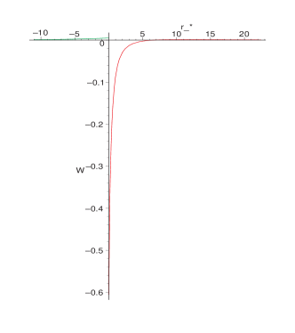
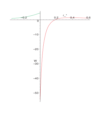
Figure 1: $r_{6}^{2}W$ plotted against $r_{*}/r_{6}$ for (left) $r_{0}=10r_{6}$, $V=1000V_{*}$, $M=0$, (right) $r_{0}=r_{6}/10$, $V=1000V_{*}$, $M=0$.

However, there is a general argument which says that there can never be an instability in this case [26]. First, we note that as (76) is simply the free wave equation in this background, it always has $\delta\psi_{3}=$ constant as a solution. In terms of the bound state problem (80), this translates into the statement that there is a zero energy $(\omega=0)$ eigenmode $\psi_{0}$ of (80) which of the same sign and is bounded everywhere; we can take it to be always positive. This zero mode $\psi_{0}$ does not vanish at the boundaries, so it is not a physical perturbation but it is still an acceptable mathematical solution of this equation.

Now assume there is a discrete spectrum of bound states $\psi_{\omega}$ with negative energy. These are our hypothetical unstable modes with $\omega^{2}<0$. We can see from the form of (80) that they go to zero as $r_{*}\to\pm\infty$. This means that they are bounded solutions and physical perturbations of our problem. The standard ‘node rule’ for the number of nodes of the eigenfunctions of the discrete bound states says that in order of increasing energy, the $n$th eigenmode has $n-1$ nodes (without including the boundary ones). Thus, the lowest negative mode $\psi_{\omega_{max}}$ must have no nodes in the sense of the above rule: we can take it to be everywhere positive.

Both $\psi_{0}$ and $\psi_{\omega_{max}}$ are solutions of the wave equation (80). By multiplying the equation for each mode by the other and taking the difference, and integrating over $r_{*}$, we can obtain the equation

$$(\psi_{\omega_{max}}\partial_{r_{*}}\psi_{0}-\psi_{0}\partial_{r_{*}}\psi_{\omega_{max}})|_{r_{*}=\pm\infty}=-\omega_{max}^{2}\int^{\infty}_{-\infty}\psi_{\omega_{max}}\psi_{0}dr_{*}$$ (87)

The left-hand side is the difference of the Wronskians calculated at the boundaries. Since the eigenmode $\psi_{0}$ approaches a positive constant at the boundaries $r_{*}=\pm\infty$, while the eigenmode $\psi_{\omega_{max}}$ goes to zero, the Wronskian vanishes at each boundary. Hence, the left-hand side is zero. On the other hand, since both $\psi_{\omega_{max}}$ and $\psi_{0}$ are supposed to be everywhere positive, the right-hand side cannot be zero unless $\omega_{max}=0$. Thus, assuming the existence of eigenmodes $\psi_{\omega}$ with $\omega^{2}<0$ produces a contradiction. Hence there can be no such modes, implying that the geometry is stable to perturbation by $\delta\psi_{3}$.

Acknowledgements

We are grateful to James Gregory, Clifford Johnson and Matt Strassler for useful discussions and to Geoffrey Potvin for bringing to our notice a typo in (4). AD is supported in part by EPSRC studentship 00800708 and by a studentship from the University of Durham. SFR is supported by an EPSRC Advanced Fellowship.

References

[1]
G. T. Horowitz and R. C. Myers, “The value of singularities,” Gen. Rel. Grav.
27 (1995) 915–919,
gr-qc/9503062.
[2]
J. Polchinski and M. J. Strassler, “The string dual of a confining
four-dimensional gauge theory,”
hep-th/0003136.
[3]
K. Pilch and N. P. Warner, “ supersymmetric renormalization group
flows from IIB supergravity,” Adv. Theor. Math. Phys. 4 (2002)
627–677,
hep-th/0006066.
[4]
I. R. Klebanov and M. J. Strassler, “Supergravity and a confining gauge
theory: Duality cascades and sb-resolution of naked singularities,”
JHEP 08 (2000) 052,
hep-th/0007191.
[5]
J. M. Maldacena and C. Nunez, “Towards the large limit of pure
super Yang Mills,” Phys. Rev. Lett. 86 (2001) 588–591,
hep-th/0008001.
[6]
A. Buchel, A. W. Peet, and J. Polchinski, “Gauge dual and noncommutative
extension of an supergravity solution,” Phys. Rev. D63 (2001)
044009,
hep-th/0008076.
[7]
N. Evans, C. V. Johnson, and M. Petrini, “The enhancon and gauge
theory/gravity RG flows,” JHEP 10 (2000) 022,
hep-th/0008081.
[8]
K. Behrndt, “About a class of exact string backgrounds,” Nucl. Phys. B455 (1995) 188–210,
hep-th/9506106.
[9]
R. Kallosh and A. D. Linde, “Exact supersymmetric massive and massless white
holes,” Phys. Rev. D 52 (1995) 7137–7145,
hep-th/9507022.
[10]
C. V. Johnson, A. W. Peet, and J. Polchinski, “Gauge theory and the excision
of repulson singularities,” Phys. Rev. D 61 (2000) 086001,
hep-th/9911161.
[11]
D. Z. Freedman and J. A. Minahan, “Finite temperature effects in the
supergravity dual of the gauge theory,” JHEP 01 (2001)
036,
hep-th/0007250.
[12]
A. Buchel, “Finite temperature resolution of the Klebanov-Tseytlin
singularity,” Nucl. Phys. B600 (2001) 219–234,
hep-th/0011146.
[13]
A. Buchel, C. P. Herzog, I. R. Klebanov, L. A. Pando Zayas, and A. A. Tseytlin,
“Non-extremal gravity duals for fractional D3-branes on the conifold,”
JHEP 04 (2001) 033,
hep-th/0102105.
[14]
S. S. Gubser, C. P. Herzog, I. R. Klebanov, and A. A. Tseytlin, “Restoration
of chiral symmetry: A supergravity perspective,” JHEP 05 (2001) 028,
hep-th/0102172.
[15]
C. P. Herzog and P. Ouyang, “Fractional D1-branes at finite temperature,”
Nucl. Phys. B610 (2001) 97–116,
hep-th/0104069.
[16]
S. S. Gubser, A. A. Tseytlin, and M. S. Volkov, “Non-Abelian 4-d black
holes, wrapped 5-branes, and their dual descriptions,” JHEP 09 (2001)
017,
hep-th/0108205.
[17]
C. V. Johnson, R. C. Myers, A. W. Peet, and S. F. Ross, “The enhançon and
the consistency of excision,” Phys. Rev. D 64 (2001) 106001,
hep-th/0105077.
[18]
K. Maeda, T. Torii, M. Narita, and S. Yahikozawa, “The stability of the shell
of d2-d6 branes in a supergravity solution,”
hep-th/0107060.
[19]
M. Bertolini, T. Harmark, N. A. Obers, and A. Westerberg, “Non-extremal
fractional branes,” Nucl. Phys. B632 (2002) 257–282,
hep-th/0203064.
[20]
E. J. Weinberg, “Black holes with hair,”
gr-qc/0106030.
[21]
M. Wijnholt and S. Zhukov, “Inside an enhancon: Monopoles and dual
Yang-Mills theory,” Nucl. Phys. B639 (2002) 343–369,
hep-th/0110109.
[22]
A. Dimitriadis, K. Maeda, S. F. Ross, and T. Torii, “Stability of the
non-extremal enhançon II,”. (To appear).
[23]
S. S. Gubser and I. Mitra, “The evolution of unstable black holes in anti-de
Sitter space,” JHEP 08 (2001) 018,
hep-th/0011127.
[24]
R. Gregory and R. Laflamme, “Black strings and p-branes are unstable,” Phys.
Rev. Lett. 70 (1993) 2837–2840,
hep-th/9301052.
[25]
C. F. E. Holzhey and F. Wilczek, “Black holes as elementary particles,” Nucl.
Phys. B380 (1992) 447–477,
hep-th/9202014.
[26]
P. Kanti, N. E. Mavromatos, J. Rizos, K. Tamvakis, and E. Winstanley,
“Dilatonic black holes in higher-curvature string gravity. II: Linear
stability,” Phys. Rev. D57 (1998) 6255–6264,
hep-th/9703192.