ITF-2002/39

SPIN-2002/22

hep-th/0207179

PERTURBATIVE CONFINEMENT

Gerard ’t Hooft

Institute for Theoretical Physics

Utrecht University, Leuvenlaan 4

3584 CC Utrecht, the Netherlands

and

Spinoza Institute

Postbox 80.195

3508 TD Utrecht, the Netherlands

e-mail: g.thooft@phys.uu.nl
internet: http://www.phys.uu.nl/~thooft/

Astract
A Procedure is outlined that may be used as a starting point for a perturbative treatment of theories with permanent confinement. By using a counter term in the Lagrangian that renormalizes the infrared divergence in the Coulomb potential, it is achieved that the perturbation expansion at a finite value of the strong coupling constant may yield reasonably accurate properties of hadrons, and an expression for the string constant as a function of the QCD $\Lambda$ parameter.

1 Introduction

In recent work[1], Greensite and Thorn described a simple procedure to produce wave functions for states that may describe stringlike features for hadrons in QCD. As an Ansatz, a wave function was taken of the form

$$\psi(\vec{x}_{1},\,\vec{x}_{2},\cdots,\vec{x}_{N-1})=A\prod_{i=1}^{N}\phi(\vec{u}_{i})\ ,$$ (1.1)

where

$$\vec{u}_{i}=\vec{x}_{i}-\vec{x}_{i-1}\quad,\qquad\vec{x}_{0},\ \vec{x}_{N}\quad\hbox{fixed.}$$ (1.2)

They then propose to use a variational principle: $\phi$ is chosen such that the total energy $\cal E$, defined by

$${\cal E}=\sum T^{\rm kin}+\sum V^{\rm Coulomb}\ ,$$ (1.3)

is minimized. Here, $V^{\rm Coulomb}$ is taken to be simply the Coulomb potential,

$$V^{\rm Coulomb}=\sum_{i}V^{\rm C}(\vec{u}_{i})\quad,\qquad V^{\rm C}(\vec{u})=-{\alpha_{s}\over|\vec{u}|}\ .$$ (1.4)

Subsequently, it is proposed to try “improved Ansätze”, and it is suspected that those wave functions that give a string like appearance will carry the lowest amounts of total energy $\cal E$.

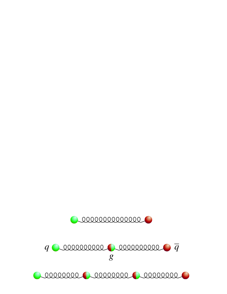
Figure 1:

The Gluon Chain Model

Some aspects of this proposal, however, are less than satisfactory. Certainly, permanent confinement is not at all a guaranteed property. If we consider the complete set of elements of Fock space, we must include all those states in which gluons do not form a chain, and therefore it is to be expected that unitarity will not hold if we restrict ourselves to chainlike states. A complete set of stringlike states could be found by replacing the Coulomb potential by a confining potential, but can one justify such a prescription in a theory where the classical limit would not exhibit any resemblance to a confinement mechanism?

In this paper, it is attempted to answer this question. Confinement should be regarded as a natural renormalization phenomenon in the infrared region of a theory. The way to deal with renormalization counter terms in the infrared is not so different from the more familiar ultraviolet renormalization. In Section 2, we explain how to look upon bare Lagrangians, renormalized Lagrangians, and how counter terms may switch position in the perturbation expansion.

In Section 3, the counter term expected for renormalizing the Coulomb potential is discussed. At this stage of the procedure, fixing the gauge condition to be the radiation gauge is crucial. There are no ghosts then, so unitarity of the procedure is evident, as long as we take for granted that the ultraviolet divergences can be handled separately by the usual methods (the ultraviolet nature of the theory is assumed not to be affected by what happens in the infrared). We then explain how to work with such counter terms (Section 4).

Working with non-gauge-invariant, non-Lorentz-invariant expressions will be cumbersome in practice, which is why we seek for a more symmetric approach. In Section 5, it is shown that gauge-invariant renormalization effects in the infrared can also easily lead to confinement. Again, the renormalization counter terms are essentially local but soft. they cannot exist as fundamental interaction terms in a quantized field theory, but they must arise as effective interactions due to higher loop contributions.

Technicalities are worked out in Section 6, and finally, it is shown that magnetic confinement could be handled in a similar fashion, although, of course, the standard Higgs mechanism is a more practical way to deal with such theories.

2 Renormalization

To illustrate our new approach, we remind the reader of the standard procedures for ultraviolet renormalization. In that case, the “bare Lagrangian”, ${\cal L}^{\rm bare}$, is rewritten as

$${\cal L}(g,\,A,\cdots)={\cal L}^{\rm bare}+\Delta{\cal L}-\Delta{\cal L}\ ,$$ (2.1)

where one subsequently interpretes the combination

$${\cal L}^{\rm renorm}(g^{\rm ren},\,A^{\rm ren})={\cal L}^{\rm bare}+\Delta{\cal L}\ ,$$ (2.2)

as the finite, “renormalized” Lagrangian. Using a regulator procedure such as, for instance, a lattice, one may allow that ${\cal L}^{\rm bare}$, the bare couplings $g$ and the bare fields $A$ become ill-defined, or ”infinite”, in the limit where the regulator vanishes ($a\downarrow 0$), but the limit should be arranged in such a way that the renormalized coupling parameters $g^{\rm ren}$ are finite, and the renormalized fields $A^{\rm ren}$ are finite operators.

$\Delta{\cal L}$ does contain infinities, but these are precisely constructed so as to cancel all infinities that one encounters in calculating the higher loop corrections, order by order in perturbation theory. In calculating these higher order corrections, one again uses ${\cal L}^{\rm renorm}$, not ${\cal L}^{\rm bare}$, because, indeed, $\Delta{\cal L}$ is again needed to cancel the subdivergences at higher orders, as one can verify explicitly.

It is important to note now that indeed we could have chosen anything for $\Delta{\cal L}$, as long as we insist that whatever we borrow to include in the “lowest order” Lagrangian ${\cal L}^{\rm renorm}$, we return when a higher loop correction is computed. The procedure pays off in particular if we manage this way to keep the higher order corrections, after having returned $\Delta{\cal L}$ together with them, as small as possible.

What does “as small as possible” mean? This is something one may dispute. The renormalization group is based on the observation that when features are computed for external momenta (and possible relevant mass terms) at a typical scale $\mu$, then the optimal choice for $\Delta{\cal L}$ depends on this scale $\mu$. For small scale transformations, the transition from one choice of $\Delta{\cal L}$ to another may not seem to be very important, but for transitions from one scale to a very much larger or smaller one, it is. The result is that the renormalized coupling strength $\alpha_{s}$ depends on $\mu$, and it may vanish (logarithmically) as $\mu\rightarrow\infty$.

There appears to be no objection against a wider use of such a procedure. If our higher order amplitudes exhibit infrared divergences, besides the ultra-violet ones, we could absorb them in $\Delta{\cal L}$ as well. This time, $\Delta{\cal L}$ is not expected to affect the coupling strengths and the field operators, but a quantity that is ideally suited to be renormalized by such terms is the effective Coulomb potential. Thus, after already having dealt with the ultraviolet divergences, we add to the “lowest order Lagrangian” ${\cal L}^{\rm renorm}$, a further term $\Delta{\cal L}$ that affects the Coulomb potential. We just borrow this term from the higher order corrections. As soon as these are calculated, we will be obliged to return the loan.

3 The Renormalized Coulomb potential

In the sequel, we refer to the usual QCD Lagrangian as ${\cal L}^{\rm bare}$, even if the ultraviolet divergences have already been taken care of. $\Delta{\cal L}$ will then only describe the new, infrared counter terms. Thus, we write

$${\cal L}^{\rm bare}=-{\textstyle{1\over 4}}F_{\mu\nu}F_{\mu\nu}-\overline{\psi}(\gamma D+m)\psi+{\cal L}^{\rm gauge-fix}+{\cal L}^{\rm ghost}+\Delta{\cal L}-\Delta{\cal L}\,.$$ (3.1)

The radiation gauge,

$$\partial_{i}A_{i}=0\ ,$$ (3.2)

is useful if questions of unitarity are to be kept under control, such as here. As usual, Latin indices $i,\,j,\cdots$ are taken to run from 1 to 3, whereas Greek indices $\mu,\,\nu,\cdots$ must run from 0 to 3 (or from 1 to 4). The color indices are of no direct concern at this stage, since all our expressions at this order are diagonal in the color indices, which is why we suppress them, for the time being. In this radiation gauge, the kinetic part of the gauge field Lagrangian will be

$${\cal L}^{\rm bare}=-{\textstyle{1\over 2}}(\partial_{\mu}A_{\nu})^{2}+{\textstyle{1\over 2}}(\partial_{\nu}A_{\nu})^{2}=-{\textstyle{1\over 2}}(\partial_{i}A_{j})^{2}+{\textstyle{1\over 2}}(\partial_{0}A_{j})^{2}+{\textstyle{1\over 2}}(\partial_{j}A_{0})^{2}\,.$$ (3.3)

Here, $A_{i}$ behaves as an ordinary dynamical variable, except for the constraint (3.2), whereas $A_{0}$ only emerges in a spacelike derivative term; its timelike derivative, $\partial_{0}A_{0}$ is absent (it cancelled out in (3.3)). Therefore, $A_{0}$ generates the instantaneous Coulomb interaction between all color charges.

The Coulomb interaction resulting from the bare Lagrangian is

$$V^{\rm Coulomb}_{q,\overline{q}}(\vec{r}\,)=-{\alpha_{s}\over|\,r|}\ .$$ (3.4)

Our procedure will be particularly important when infinite infrared corrections show up. This is exactly what we expect in a theory with confinement. We do not intend to “prove” permanent confinement here. Such a ‘proof’, or at least some justification for its assumption, is assumed to be given elsewhere.[2] We take for granted now that the renormalized Coulomb potential will be a confining one. Typically, what is needed is an ‘effective’ potential that is diagonal in the color indices, and takes up the new form

$$V^{\rm ren}_{q,\overline{q}}(\vec{r}\,)=-{\alpha_{s}\over|\,r|}+\varrho|\,r|\ ,$$ (3.5)

where $\varrho$ is an effective string constant. Notive that the signs here are chosen in such a way that the Coulomb force keeps a constant sign. The presence of a zero in Eq.(3.5) is of no significance.

The familiar Coulomb term, Eq.(3.4), obeys the Laplace equation

$$\vec{\partial}^{\,2}V^{\rm Coulomb}(\vec{r})=4\pi\alpha_{s}\,\delta^{3}(\vec{r})\ ,$$ (3.6)

whereas the extra term in Eq.(3.5) obeys the Laplace equation

$$\vec{\partial}^{\,2}(\varrho|\,r|)={2\varrho\over|\,r|}\quad;\qquad\vec{\partial}^{\,2}\left({2\varrho\over|\,r|}\right)=-8\pi\varrho\,\delta^{3}(\vec{r})\ .$$ (3.7)

Therefore, in 3 dimensional Fourier space, the renormalized Coulomb potential is[3]

$$V^{\rm ren}(\vec{k})=-{4\pi\alpha_{s}\over\vec{k}^{2}}-{8\pi\varrho\over\vec{k}^{4}}\,,$$ (3.8)

so that the Laplace equation for the renormalized potential will have to be constructed from

$${\vec{k}^{4}\over\vec{k}^{2}+2\varrho/\alpha_{s}}\,V^{\rm ren}=-4\pi\alpha_{s}\delta^{3}(\vec{r})$$ (3.9)

(Here, an admittedly ugly mixed Fourier-coordinate space notation was admitted). Because of the extra term $2\varrho/\alpha_{s}$, the renormalized Lagrangian should contain the following, modified Coulomb term:

$${\cal L}^{\rm bare}+\Delta{\cal L}=\dots+{\textstyle{1\over 2}}\partial_{j}A_{0}\left(1-{2\varrho/\alpha_{s}\over\vec{k}^{2}+2\varrho/\alpha_{s}}\right)\partial_{j}A_{0}\ ,$$ (3.10)

so that $\Delta{\cal L}$ must be chosen to be

$$\Delta{\cal L}=-{\textstyle{1\over 2}}\partial_{j}A_{0}\,{2\varrho/\alpha_{s}\over\vec{k}^{2}+2\varrho/\alpha_{s}}\,\partial_{j}A_{0}\ .$$ (3.11)

In coordinate space, this takes the form

$$\int\Delta{\cal L}(\vec{x},t)\,{\rm d}^{3}\vec{x}=-{\textstyle{1\over 2}}\int{\rm d}^{3}\vec{x}\int{\rm d}^{3}\vec{x}^{\prime}\,\partial_{j}A_{0}(\vec{x})\,G(\vec{x}-\vec{x}^{\prime})\,\partial_{j}A_{0}(\vec{x}^{\prime})\ ,$$

$${\rm where}\qquad G(\vec{r})={8\pi\varrho\over\alpha_{s}}\,{1\over|\,r|}\,e^{-\sqrt{2\varrho/\alpha_{s}}\,|\,r|}\ .$$ (3.12)

Note that $G(\vec{x}-\vec{x}^{\prime})$ is fairly ‘soft’, both in the infrared (where it decays exponentially), and in the ultraviolet (where it is integrable and considerably weaker than the Dirac delta function of the canonical term). On the other hand, this term cancels the canonical term completely at $\vec{k}\rightarrow 0$.

Figure 2: The one-loop corrections to the gluon propagator: the gluon, the quark and the ghost term (the minus signs are due to the Fermi statistics of the last two; the last diagram, the ghost, actually does not contribute in the radiation gauge).

4 Infinite infrared renormalization

In the standard perturbative approach, the one-loop correction to the gluon self-energy is infrared divergent. The self-energy correction from the diagrams of the type of Figure 2 is

$$C\,g^{2}(k^{2}\delta_{\mu\nu}-k_{\mu}k_{\nu})\log{1\over k^{2}}\ .$$ (4.1)

It would produce a correction term to the Coulomb potential of the form $\log(1/\vec{k}^{2})$ times that term. The divergence at $|\vec{k}|\rightarrow\infty$ is the standard type that is to be taken care of by ultraviolet renormalization. It is the divergence near $|\vec{k}|\rightarrow 0$, which goes as $2C\log(1/|\vec{k}|$, that we now wish to regulate. The counter term produced by Eqs. (3.11) and (3.12) has the form

$$-{\mu^{2}\over\vec{k}^{\,2}+\mu^{2}}(k^{2}\delta_{\mu\nu}-k_{\mu}k_{\nu})\quad;\qquad\mu^{2}\equiv 2\varrho/\alpha_{s}\ .$$ (4.2)

The coefficient $\mu$ could now be required to be adjusted in such a way that Eq. (4.2) cancels Eq. (4.1) “as well as possible”.

Actually, the first order correction is not quite Eq. (4.1), because the first order Lagrangian was modified by the $\Delta{\cal L}$ term. The diagram that has to be calculated actually is the one of Figure 3, where the shaded area denotes the effects from the confining potential, Eq. (3.5). The effects this is expected to have on calculating the higher order corrections to the Coulomb potential are sketched in Figure 4.

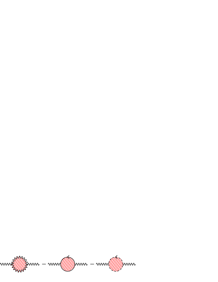
Figure 3: The one-loop corrections to the gluon propagator in the presence of a confining potential.

Although the counter term (3.11) is sufficient to produce the above effects at higher order, one could also think of replacing it by some gauge-invariant, or nearly gauge-invariant expression, such as

$$\Delta{\cal L}=+{\textstyle{1\over 4}}\int F_{\mu\nu}(\vec{x},t)G(\vec{x}-\vec{x}^{\prime})F_{\mu\nu}(\vec{x}^{\prime},t)\,{\rm d}^{3}\vec{x}^{\prime} \ ;$$ (4.3)

$$G(\vec{r})={8\pi\over\alpha_{s}}\,{1\over|\vec{r}\,|}\,e^{-\sqrt{2\varrho/\alpha_{s}}{|\vec{r}\,|}} \ .$$ (4.4)

Notice that this is only gauge-invariant in the Abelian case. In non-Abelian theories, $G$ must be replaced by a gauge-invariant path-ordered expression.

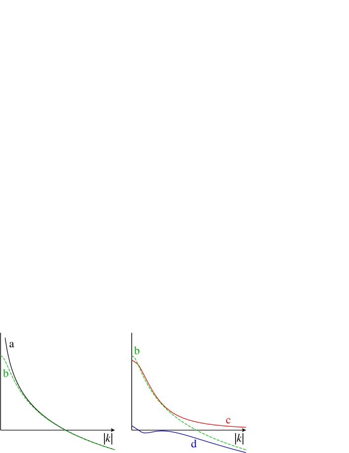
Figure 4: The one-loop corrections to the gluon potential. $a$) The standard pure logarithm (in the case of massless flavors only). $b$) Estimate of the modification due to the confinement of the gluons inside the loop; the singularity at $k\rightarrow 0$ is exected to disappear. $c$) The counter term, Eq. (4.2). $d$) The expected total one-loop correction, after subtraction of the counter term.

On the other hand, in Eq. (4.4), one could actually allow for more general expressions such that the higher order corrections to the Coulomb potential cancel out completely. This would not turn all higher order corrections to zero, since we limit ourselves to counter terms that are strictly local in time (see Eq. (4.3).

Note that, in all cases, the $\Delta{\cal L}$ that was inserted at zeroth order, is borrowed from the correction at higher order (typically the one-loop order), where it is returned, so as to render these correction terms as small as possible. There is considerable freedom in choosing $\Delta{\cal L}$, allowing it to be non-local in space, but we do insist that it stays local in time. This will guarantee that the Lagrangian we work with will always produce unitary $S$-matrices at all stages. It also guarantees that, if the first loop corrections are small, also the higher loop corrections stay small, just like the situation we have in conventional renormalization procedures, where this can be proven using dispersion relations.[4]

5 Gauge-invariant counter terms

The procedure described in the previous section had the disadvantage that gauge-invariance is lost. Locality of the counter term in time, and the fact that it is cancelled at higher order, should minimize the damage done, but still it might be preferable to keep the infrared counter terms gauge-invariant from the start. Eq.(4.3) is a step in the right direction, but then, the non-local kernel (4.4) should also be made gauge-invariant, which is somewhat complicated in practice. It would be easier if we could fabricate the counter terms in such a way that the lowest order Lagrangian obtains the form

$${\cal L}^{\rm renorm.}\ =\ {\cal L}^{\rm bare}+\Delta{\cal L}\ =\ f(-{\textstyle{1\over 4}}F_{\mu\nu}F_{\mu\nu})\,.$$ (5.1)

We have not yet worked out the formal scheme of correcting for this modification at higher orders, but it might be doable. The point that will be made in this section is that, with certain minor modifications from the canonical theory $f(x)=x$, which only need to be sizable at small values of $x$, theories can be obtained that provide for rigorously confining potentials.

To demonstrate this, we first rewrite[5] the Lagrangian (5.1), including a possible external source, as

$${\cal L}(A,\phi)=-{\textstyle{1\over 4}}Z(\phi)F_{\mu\nu}F_{\mu\nu}-V(\phi)+J_{\mu}A_{\mu}\,.$$ (5.2)

As the field $\phi$ was given no kinetic term here, the Lagrange equations simply demand that we extremize with respect to the $\phi$ field, so that equivalence with Lagrangian (5.1) is easy to establish. In the following, we consider the static situation, and by concentrating on one color excitation only, we ignore the non-Abelian terms that otherwise could arise.

To solve the static case, with fixed sources $J_{0}$, the complete equations are easier to handle if we first solve the equations for the fields $A_{\mu}$. One gets

$$\partial_{i}D_{i}=\varrho=J_{0}\ ;$$ (5.3)

$$\vec{D}=Z(\phi)\vec{E}\quad,\quad E_{i}= -\partial_{i}A_{0}\ {}.$$ (5.4)

By adding to the Lagrangian (5.2) a term

$$-{1\over 2Z}(Z\partial_{i}A_{0}+D_{i})^{2}\,,$$ (5.5)

where $D_{i}$ is a free variable, we see that what has to be extremized is the Hamiltonian

$${\cal H}\ =\ D_{i}\dot{A_{i}}-{\cal L}\ =\ {\textstyle{1\over 2}}\,{\vec{D}^{2}\over Z(\phi)}+V(\phi)+J_{0}A_{0}\ ,$$ (5.6)

which is just $-{\cal L}$ in the static case, with Eq. (5.3) as a constraint.

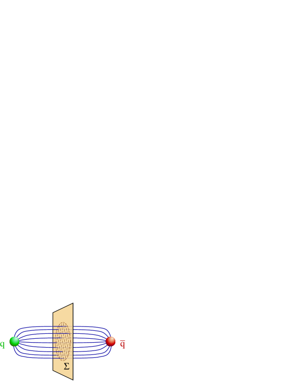
Figure 5: The quark-antiquark vortes in a classical model. Shown are the $\vec{D}$ field lines (whose divergence is controlled by the quark sources), and a sheet crosssecting these lines. Only inside the surface $\SS$ (indicated as a shaded ellipse) they differ appreciably from zero.

Let us assume momentarily that the minimum energy configuration (in the presence of quark sources) is that of a vortex, as is illustrated in Figure 5. The $\vec{D}$ field lines may spread over a surface area $\SS$. In that case, the predominant field strength $\overline{D}$ is

$$\overline{D}\simeq{Q^{\rm quark}\over\SS}\quad\rightarrow\qquad\SS={Q\over\overline{D}}\ ,$$ (5.7)

where $Q$ stands for the (Abelian) charge of a quark. The energy per unit of length is

$${{\cal E}\over L}\equiv\varrho^{\rm string}\quad=\quad\min_{\SS}\left(\SS\,U(\overline{D})\right)\quad=\quad\min_{D}\left(Q{U(D)\over D}\right)\,.$$ (5.8)

If, indeed, Eq. (5.8) has a non-vanishing minimum, then Fig. 5 correctly represents the configuration with optimal energy. Note that, in the Maxwell case, one would have:

$$U(D)={\textstyle{1\over 2}}\,D^{2}\ ,\qquad\hbox{(Maxwell)},$$ (5.9)

so then there is no non-vanishing minimum, so that the field lines spread out as usual. The minimum exists if, for low values of $D$, its energy goes as

$$U(\vec{D})\downarrow\varrho|\vec{D}|\ ,$$ (5.10)

which, for simplicity, we take to be the case as $|\vec{D}|\rightarrow 0$. For large $\vec{D}$, we expect asymptotic freedom to come into effect, so that the Maxwellian behaviour (5.9) is resumed. For simplicity, also, we take $Q=1$, so that $\varrho=\varrho^{\rm string}$.

Thus, we see that Eq. (5.10) is sufficient to obtain the effect of linear vortex formation. We now investigate what this may imply for the function $f(x)$ in Eq.(5.1).

6 An exercise in Legendre transformations

First, one has to establish the required relation between $Z(\phi)$ and $V(\phi)$. extremizing with respect to $\phi$ implies

$${\partial\over\partial\phi}\left({{\textstyle{1\over 2}}D^{2}\over Z(\phi)}+V(\phi)\right)=0\quad\rightarrow\quad{\textstyle{1\over 2}}D^{2}=-{\partial V\over\partial(1/Z)}\ .$$ (6.1)

Regarding $U$ as a function of ${\textstyle{1\over 2}}D^{2}$ and $\phi$, we have

$${\rm d}U={\textstyle{1\over 2}}D^{2}{\rm d}{1\over Z}+{1\over Z}{\rm d}({\textstyle{1\over 2}}D^{2})+{\rm d}V={1\over Z}\,{\rm d}({\textstyle{1\over 2}}D^{2})\,.$$ (6.2)

In the domain where we require Eq.(5.10) to hold, we therefore have

$${1\over Z}={{\rm d}U\over{\rm d}({\textstyle{1\over 2}}D^{2})}\quad\approx\quad{{\rm d}(\varrho D)\over{\rm d}{\textstyle{1\over 2}}D^{2}}={\varrho\over D}\ .$$ (6.3)

From Eq. (6.1), one deduces

$$V=-\int{\textstyle{1\over 2}}D^{2}\,{\rm d}\left({1\over Z}\right)\quad\approx\quad{\textstyle{1\over 2}}\varrho\,D={\textstyle{1\over 2}}\varrho^{2}Z\ .$$ (6.4)

At large values of $D$, we expect the Maxwellian behaviour (5.9), so that there

$$Z\rightarrow 1\quad:\qquad{\partial V\over\partial Z}\rightarrow\infty\ .$$ (6.5)

Whether or not $V$ itself tends to a constant there, or to infinity, is not very important. All in all, we expect the behaviour sketched in Fig. 6.

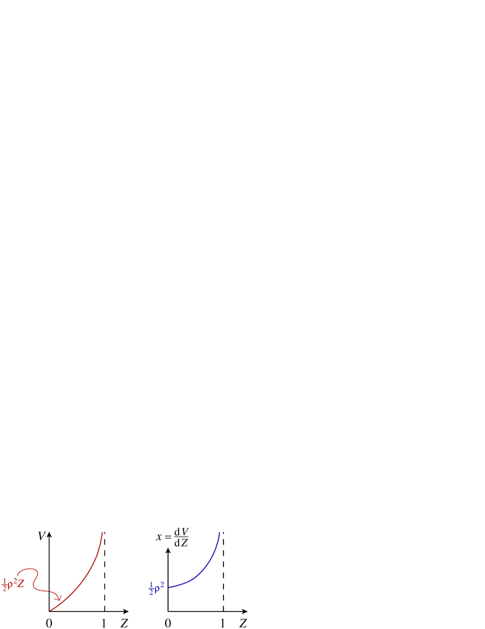
Figure 6: The relation between $Z(\phi)$ and $V(\phi)$ producing confinement, and the resulting relation between $x$ and $Z$.

With this result we now return to Eq. (5.2), which we rewrite as

$${\cal L}=Zx-V\quad,\qquad x=-{\textstyle{1\over 4}}F_{\mu\nu}F_{\mu\nu}\,.$$ (6.6)

Extremizing this with respect to $\phi$ gives

$${\partial{\cal L}\over\partial\phi}=0\ \rightarrow\ {\partial V\over\partial Z}=x=-{\textstyle{1\over 4}}F_{\mu\nu}F_{\mu\nu}={\textstyle{1\over 2}}E^{2}\ .$$ (6.7)

This allows us to eliminate $\phi$ by writing

$${\rm d}{\cal L}=x{\rm d}Z+Z{\rm d}x-{\rm d}V=Z{\rm d}X\ ;\quad Z={{\rm d}{\cal L}\over{\rm d}x}\ .$$ (6.8)

Combining Eq. (6.4) with (6.7), we find the relation between $x$ and $Z$. Inverting this, using the relation $Z(x)$, we find ${\cal L}(x)$, and we see that at

$$x={\textstyle{1\over 2}}E^{2}={\textstyle{1\over 2}}\varrho^{2}\ ,\quad{{\rm d}{\cal L}\over{\rm d}x}=0\ .$$ (6.9)

Apparently, the function $f(x)$, which in the Maxwell case is just equal to $x$, must now have an extremum at the value (6.9).

This establishes the function $f(x)$ for all $x\geq{\textstyle{1\over 2}}\varrho^{2}$. How exactly the function continues for $x$ smaller than that value is of no direct consequence for the confinement mechanism; of course $f$ must approach the classical value $x$ at large $|x|$. Figure 7 shows the possibilities.

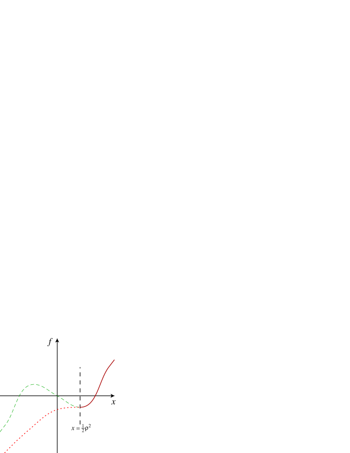
Figure 7: Different possibilities for the function $f(x)$ yielding confinement. The behaviour to the right of the extremum (solid curve) must be as indicated.

Finally, let us derive a curve $f(x)$ that would produce magnetic confinement, i.e. the Higgs mechanism. We perform a dual transformation:

$$G_{\mu\nu}\equiv Z(\phi)\,{\textstyle{1\over 2}}\,\varepsilon_{\mu\nu\alpha\beta}F_{\alpha\beta}=Z\,\tilde{F}_{\mu\nu}\,.$$ (6.10)

In the source-free case, the Maxwell equation $\partial_{\mu}(Z\,F_{\mu\nu})=0$ implies

$$\partial_{\alpha}G_{\beta\gamma}+\partial_{\beta}G_{\gamma\alpha}+\partial_{\gamma}G_{\alpha\beta}=0\,,$$ (6.11)

so that one may write

$$G_{\mu\nu}=\partial_{\mu}B_{\nu}-\partial_{\nu}B_{\mu}\,,$$ (6.12)

and the equations are associated to the Lagrangian

$${\cal L}(B,\phi)={-{\textstyle{1\over 4}}G_{\mu\nu}G_{\mu\nu}\over Z(\phi)}-V(\phi)\,.$$ (6.13)

Electric confinement for the $F$ and $A$ fields implies magnetic confinement for the $G,$ and $B$ fields. We see that $Z$ is replaced by $1/Z$. Plugging in the same equation (6.4), $V={\textstyle{1\over 2}}\varrho^{2}\,Z$, as $Z\rightarrow 0$, we see a prescribed behaviour when $y\equiv{\textstyle{1\over 4}}G_{\mu\nu}G_{\mu\nu}=-x={\textstyle{1\over 2}}B^{2}$ is positive:

$${\cal L}(B)=-{y\over Z}-V\ ;$$ (6.14)

$${{\rm d}{\cal L}\over{\rm d}\phi}=0\quad\rightarrow\quad Z=\sqrt{y\over{\textstyle{1\over 2}}\varrho^{2}}\quad; \ V=\sqrt{{\textstyle{1\over 2}}\varrho^{2}\,y}\ ;$$ (6.15)

$${\cal L}\rightarrow-\varrho\sqrt{2y}=-\varrho|\vec{B}|\ .$$ (6.16)

The resulting function $f(x)=f(-y)$ is sketched in Figure 8.

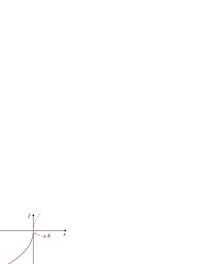
Figure 8: The function $f(x)$ in the case of magnetic confinement.

7 Discussion

Permanent confinement of electric sources is not necessarily a purely non-perturbative quantum phenomenon. One can choose between classical, reasonably looking Lagrangians of various kinds that produce this effect. These Lagrangians are non-renormalizable, and this means they cannot be used to describe the theory in the far ultraviolet. We must assume that the soft, infrared divergent correction terms are due to quantum corrections, but they do not have to be non-perturbative quantum corrections. The counter terms used in the first chapters of this contribution, are only slightly non-local in space, while all are local in time. Arguments that are very similar to renormalization group arguments can be applied to conclude that terms of this kind, which become dominating in the far infrared, necessarily arise when we scale to longer distances.

References

- [1] J. Greensite and Ch.B. Thorn, Gluon Chain Model of the Confining Force, hep-ph/0112326.
-
[2]
G. ’t Hooft, “Gauge Theories with Unified Weak, Electromagnetic and
Strong Interactions”, E.P.S. Int. Conf. on High Energy Physics,
Palermo 23-28 June 1975; see also papers reprinted in:
G. ’t Hooft, “Under the spell of the gauge principle”, Advanced
Series in Mathematical Physics 19 (1994), Editors: H.
Araki et al. (World Scientific, Singapore), or: G. ’t Hooft,
Phys. Scripta 24 (1981) 841;
Nucl. Phys. B190 (1981) 455.
See also: A.M. Polyakov, Nucl. Phys. B120 (1977) 429. - [3] Quartic poles were brought in connection with confining potentials long ago, e.g.: J. Kogut and L. Susskind, Phys. Rev. D9 (1974) 3501.
- [4] G. ’t Hooft and M. Veltman, ”DIAGRAMMAR”, CERN Report 73/9 (1973), reprinted in ”Particle Interactions at Very High Energies, Nato Adv. Study Inst. Series, Sect. B, vol. 4b, p. 177.
- [5] G. ’t Hooft, in Proceedings of the Colloqium on ”Recent Progress in Lagrangian Field Theory and Applications”, Marseille, June 24-28, 1974, ed. by C.P. Korthals Altes, E. de Rafael and R. Stora.