hep-th/0207177

TU-664

Novel construction of boundary states in coset conformal field theories
Hiroshi Ishikawa and Taro Tani
Department of Physics, Tohoku University
Sendai 980-8578, JAPAN

We develop a systematic method to solve the Cardy condition for the coset conformal field theory $G/H$. The problem is equivalent to finding a non-negative integer valued matrix representation (NIM-rep) of the fusion algebra. Based on the relation of the $G/H$ theory with the tensor product theory $G\times H$, we give a map from NIM-reps of $G\times H$ to those of $G/H$. Our map provides a large class of NIM-reps in coset theories. In particular, we give some examples of NIM-reps not factorizable into the $G$ and the $H$ sectors. The action of the simple currents on NIM-reps plays an essential role in our construction. As an illustration of our procedure, we consider the diagonal coset $SU(2)_{5}\times SU(2)_{3}/SU(2)_{8}$ to obtain a new NIM-rep based on the conformal embedding $su(2)_{3}\oplus su(2)_{8}\subset sp(6)_{1}$.

1 Introduction

The study of the boundary conditions in rational conformal field theories (RCFTs) has been attracted much attention since the pioneering work by Cardy [1]. It is now recognized that the requirement of the mutual consistency of the boundary conditions, which is known as the sewing relations [2, 3], is so severe that the number of the possible solutions is finite if we keep the chiral algebra of RCFT at the boundaries [1, 2, 3, 4, 5, 6, 7, 8, 9, 10]. The Cardy condition [1] is one of the sewing relations, which expresses the consistency of the annulus amplitudes without insertion of vertex operators. The problem of solving the Cardy condition is, under the assumption of the completeness [4], reduced to the study of the non-negative integer valued matrix representation (NIM-rep) of the fusion algebra[8, 11, 12].

In the context of string theory, the existence of the boundaries on the worldsheet means the presence of $D$-branes. Since the (super) conformal invariance on the worldsheet is necessary for the consistency of string theory, the possible boundary conditions are those preserving the conformal invariance and we have boundary CFTs. The classification of the possible $D$-branes is therefore equivalent with the classification of the conformal boundary conditions in a given CFT. Although RCFTs describe only some specific points in the moduli space of the string backgrounds, we can obtain insights into the stringy nature of $D$-branes from the study of the boundary conditions in RCFTs.

The coset CFT [13] is an important class of RCFTs, which contains in particular the minimal models. The coset theories are considered to be the building blocks of generic RCFTs. Therefore it is of fundamental importance to investigate and classify the boundary conditions allowed in the coset theories. This problem has been studied by several groups [14, 15, 16, 17, 18, 19, 20, 21, 22, 23]. The issue of the classification is however not completely answered yet.

In this paper, we start a systematic study toward the classification of the boundary conditions in the coset theories. Based on the relation of the coset theory $G/H$ with the tensor product theory $G\times H$, we show that any NIM-rep of the $G\times H$ theory yields a NIM-rep of the $G/H$ theory. This map from $G\times H$ to $G/H$ enables us to construct a large class of NIM-reps in the $G/H$ theory. In particular, we can obtain some examples of NIM-reps not factorizable into the $G$ and the $H$ sectors. The construction in this paper generalizes that given in the previous work by one of the present authors [18], in which the resulting NIM-reps of the $G/H$ theory are only of the factorizable form. Our map is nothing but the NIM-rep version of the map for the modular invariants of the $G\times H$ and the $G/H$ theories obtained in [24].

The action of the simple currents [25, 26] on generic NIM-reps [18, 27] plays an essential role in our construction. Namely, it is shown that we need appropriate identifications and selection rules for the Cardy states of $G\times H$, which are generated by the action of the simple currents on the Cardy states, to obtain a NIM-rep of $G/H$. These brane identifications and brane selection rules are the counterparts of the field identification and the selection rule of the coset theories, and has been first observed in [18].

The organization of this paper is as follows. In the next section, after reviewing some basic facts about the boundary states in RCFTs (Section 2.1), we develop the tools necessary in our construction of the NIM-reps in coset theories. First, we argue the action of the simple currents on generic NIM-reps in RCFTs and give the definition of the simple current group for NIM-reps (Section 2.2). Next, we explain methods to construct a NIM-rep from a given one: the use of the simple currents and conformal embeddings (Section 2.3). In Section 3, we discuss the NIM-reps in tensor product theories. Applying the methods developed in Section 2.3, we give some nontrivial NIM-reps in the $SU(2)_{k}\times SU(2)_{l}$ theory. In Section 4, we turn to coset theories and give a map for NIM-reps of the $G\times H$ and the $G/H$ theories. The necessary identifications and selection rules for the Cardy states of the $G\times H$ theory is described in terms of the simple current groups for NIM-reps obtained in Section 2.2 and the field identification currents of the coset theory. As an illustrative example for our procedure, we consider the diagonal coset $SU(2)_{k}\times SU(2)_{l}/SU(2)_{k+l}$ to obtain a NIM-rep not factorizable into the numerator and the denominator sectors. The final section is devoted to some discussions.

2 Boundary states in rational conformal field theories

2.1 NIM-reps in RCFTs

In this subsection, we review some results on the boundary states in rational conformal field theories (RCFTs).

The most important ingredient of a RCFT is a chiral algebra $\mathcal{A}$, which is the Virasoro algebra or an extension thereof. We denote by $\mathcal{I}$ the set of all the possible irreducible representations of $\mathcal{A}$. For a RCFT, $\mathcal{I}$ is a finite set. In the bulk theory, we have a pair of algebras $\mathcal{A}$ and $\tilde{\mathcal{A}}$, which correspond to the holomorphic and the anti-holomorphic sectors, respectively. In the presence of boundaries, $\mathcal{A}$ and $\tilde{\mathcal{A}}$ are related with each other via appropriate boundary conditions. We restrict ourselves to the case of rational boundary conditions, which preserve the chiral algebra $\mathcal{A}$ at the boundary. Since $\mathcal{A}$ includes the Virasoro algebra, the rational boundary condition keeps the conformal invariance at the boundary and yields a boundary CFT.

A boundary state $|\alpha\rangle$ is characterized by the following equation

$$(W_{n}-(-1)^{h}\widetilde{W}_{-n})|\alpha\rangle=0.$$ (2.1)

Here $W$ and $\widetilde{W}$ are the currents of $\mathcal{A}$ and $\tilde{\mathcal{A}}$, respectively. $h$ is the conformal dimension of the currents: $h=2$ for the Virasoro algebra and $h=1$ for the affine Lie algebras. The building blocks of the boundary states are the Ishibashi states $|\mu\rangle\!\rangle$ ($\mu\in\mathcal{I}$) [28]. We normalize the Ishibashi states as follows,

$$\langle\!\langle\mu|\tilde{q}^{H_{c}}|\mu^{\prime}\rangle\!\rangle=\delta_{\mu\mu^{\prime}}\frac{1}{S_{0\mu}}\chi_{\mu}(-1/\tau)=\delta_{\mu\mu^{\prime}}\sum_{\nu\in\mathcal{I}}\frac{S_{\mu\nu}}{S_{0\mu}}\chi_{\nu}(\tau)=\delta_{\mu\mu^{\prime}}(\chi_{0}(\tau)+\cdots),$$ (2.2)

where $\tilde{q}=e^{-2\pi i/\tau}$. $H_{c}=\frac{1}{2}(L_{0}+\tilde{L}_{0}-\frac{c}{12})$ is the closed string Hamiltonian and $c$ is the central charge of the theory. $\chi_{\mu}$ is the character of the representation $\mu\in\mathcal{I}$, and its modular transformation reads

$$\chi_{\mu}(-1/\tau)=\sum_{\nu\in\mathcal{I}}S_{\mu\nu}\chi_{\nu}(\tau).$$ (2.3)

‘$0$’ stands for the vacuum representation. The normalization (2.2) corresponds to the following scalar product in the space of the boundary states [8]

$$\langle\alpha||\beta\rangle=\lim_{q\rightarrow 0}q^{\frac{c}{24}}\langle\alpha|\tilde{q}^{H_{c}}|\beta\rangle,$$ (2.4)

where $q=e^{2\pi i\tau}$.

We denote by $\mathcal{V}$ the set labeling the boundary states. A generic boundary state $|\alpha\rangle(\alpha\in\mathcal{V})$ satisfying the boundary condition (2.1) is a linear combination of the Ishibashi states

$$|\alpha\rangle=\sum_{\mu\in\mathcal{E}}{\psi_{\alpha}}^{\mu}|\mu\rangle\!\rangle,\quad\quad\alpha\in\mathcal{V}.$$ (2.5)

Here $\mathcal{E}$ is a set labeling the Ishibashi states allowed in the model. In general, $\mathcal{E}$ does not contain all the elements appearing in the set $\mathcal{I}$ of the possible representations. Rather, $\mathcal{E}$ is a set distinct from $\mathcal{I}$ since the multiplicity of a representation $\mu$ in $\mathcal{E}$ can be greater than 1, as is seen in the $su(2)$ $D_{\text{even}}$ invariant.

The coefficients ${\psi_{\alpha}}^{\mu}$ together with the sets $\mathcal{E}$ and $\mathcal{V}$ should be chosen appropriately for the mutual consistency of the boundary states. Consider the annulus amplitude between two boundary states $|\alpha\rangle$ and $|\beta\rangle$,

$$Z_{\alpha\beta}=\langle\beta|\tilde{q}^{H_{c}}|\alpha\rangle=\sum_{\nu\in\mathcal{E},\mu\in\mathcal{I}}{\psi_{\alpha}}^{\nu}\frac{S_{\mu\nu}}{S_{0\nu}}\overline{{\psi_{\beta}}^{\nu}}\,\chi_{\mu}(\tau),\quad\quad\alpha,\beta\in\mathcal{V}.$$ (2.6)

We denote by $n_{\mu\alpha}{}^{\beta}$ the multiplicity of the representation $\mu\in\mathcal{I}$ in $Z_{\alpha\beta}$,

$${n_{\mu\alpha}}^{\beta}=\sum_{\nu\in\mathcal{E}}{\psi_{\alpha}}^{\nu}\frac{S_{\mu\nu}}{S_{0\nu}}\overline{{\psi_{\beta}}^{\nu}}=\sum_{\nu\in\mathcal{E}}{\psi_{\alpha}}^{\nu}\gamma^{(\mu)}_{\nu}\overline{{\psi_{\beta}}^{\nu}},$$ (2.7)

where $\displaystyle\gamma^{(\mu)}_{\nu}$ is the generalized quantum dimension

$$\gamma^{(\mu)}_{\nu}=\frac{S_{\mu\nu}}{S_{0\nu}}.$$ (2.8)

Clearly, ${n_{\mu\alpha}}^{\beta}$ takes non-negative integer values for consistent boundary states. In addition to this, ${n_{0\alpha}}^{\beta}=\delta_{\alpha\beta}$ since the vacuum is unique. We call this set of conditions the Cardy condition and the boundary states satisfying these conditions the Cardy states [1]. In terms of the matrix notation

$${(\psi)_{\alpha}}^{\mu}={\psi_{\alpha}}^{\mu},\quad{(n_{\mu})_{\alpha}}^{\beta}={n_{\mu\alpha}}^{\beta},\quad\gamma^{(\mu)}=\text{diag}(\gamma^{(\mu)}_{\nu}),$$ (2.9)

the Cardy condition is summarized as follows:

$$\begin{split}n_{\mu}&=\psi\gamma^{(\mu)}\psi^{\dagger}\quad\in\mathrm{Mat}(\lvert\mathcal{V}\rvert,\mathbb{Z}_{\geq 0}),\\ n_{0}&=\psi\psi^{\dagger}=1.\end{split}$$ (2.10)

Here $\mathrm{Mat}(m,\mathbb{Z}_{\geq 0})$ is the set of $m\times m$ matrices with non-negative integer entries.

So far, the number of the independent Cardy states $\lvert\mathcal{V}\rvert$ is not specified. Hereafter, we assume that the number of the Cardy states is equal to the number of the Ishibashi states [4]

$$\lvert\mathcal{V}\rvert=\lvert\mathcal{E}\rvert\quad\quad\text{(completeness)}.$$ (2.11)

If this holds, $\psi$ is a square matrix, and the Cardy condition (2.10) means that $\psi$ is unitary. The situation is quite analogous to the Verlinde formula [29]

$${\mathcal{N}_{\mu\nu}}^{\rho}=\sum_{\lambda\in\mathcal{I}}\frac{S_{\mu\lambda}S_{\nu\lambda}\overline{S_{\rho\lambda}}}{S_{0\lambda}}=\sum_{\lambda\in\mathcal{I}}S_{\nu\lambda}\gamma^{(\mu)}_{\lambda}\overline{S_{\rho\lambda}},$$ (2.12)

where ${\mathcal{N}}_{\mu\nu}{}^{\rho}$ is the fusion coefficient $(\mu)\times(\nu)=\sum_{\rho\in\mathcal{I}}{\mathcal{N}}_{\mu\nu}{}^{\rho}(\rho)$. In the matrix notation

$$(N_{\mu})_{\nu}{}^{\rho}={\mathcal{N}}_{\mu\nu}{}^{\rho},$$ (2.13)

the above formula can be written as

$$\begin{split}{N}_{\mu}&=S\gamma^{(\mu)}S^{\dagger}\quad\in\mathrm{Mat}(\lvert\mathcal{I}\rvert,\mathbb{Z}_{\geq 0}),\\ {N}_{0}&=SS^{\dagger}=1.\end{split}$$ (2.14)

From the associativity of the fusion algebra, one can show that $N_{\lambda}$ satisfies the fusion algebra

$$N_{\mu}N_{\nu}=\sum_{\rho\in\mathcal{I}}{\mathcal{N}}_{\mu\nu}{}^{\rho}N_{\rho}.$$ (2.15)

Applying the Verlinde formula (2.14) to both sides, one obtains

$$\gamma^{(\mu)}\gamma^{(\nu)}=\sum_{\rho\in\mathcal{I}}{\mathcal{N}}_{\mu\nu}{}^{\rho}\gamma^{(\rho)}.$$ (2.16)

The generalized quantum dimension $\{\gamma^{(\mu)}_{\lambda}|\,\lambda\,\text{fixed}\}$ is therefore a one-dimensional representation of the fusion algebra. If we use $\psi$ instead of $S$ in the Verlinde formula, we obtain $n_{\mu}$. Hence, $n_{\mu}$, as well as $N_{\mu}$, satisfies the fusion algebra

$$n_{\mu}n_{\nu}=\sum_{\rho\in\mathcal{I}}{\mathcal{N}}_{\mu\nu}{}^{\rho}n_{\rho}.$$ (2.17)

The Cardy condition (2.10) together with the assumption of completeness (2.11) implies that $\{n_{\lambda}\}$ forms a non-negative integer matrix representation (NIM-rep) of the fusion algebra [8].

For each set of the mutually consistent boundary states, we have a NIM-rep $\{n_{\mu}|\,\mu\in\mathcal{I}\}$ of the fusion algebra. The simplest example is the regular NIM-rep

$$\begin{split}&\psi=S\quad(\mathcal{E}=\mathcal{V}=\mathcal{I}),\\ &n_{\mu}=N_{\mu},\end{split}$$ (2.18)

which corresponds to the diagonal modular invariant and exists in any RCFT. However, the converse is in general not true. There are many ‘unphysical’ NIM-reps that do not correspond to any modular invariant [12]. The typical example is the tadpole NIM-rep $T_{n}$ of $su(2)_{2n-1}$ [11, 8]. This fact shows that the Cardy condition is not a sufficient but a necessary condition for consistency.

2.2 Action of simple currents

We next argue the action of the simple currents on NIM-reps, which is of fundamental importance in the construction of boundary states in coset CFTs [18, 27].

A simple current $J$ of a RCFT is a representation whose fusion with the other representations induces a permutation $\mu\mapsto J\mu$ of $\mathcal{I}$ [25, 26],

$$(J)\times(\mu)=(J\mu).$$ (2.19)

The set of all the simple currents forms an abelian group which we denote by $G_{\mathrm{sc}}$,

$$G_{\mathrm{sc}}=\{J|\,\,\text{simple currents}\}.$$ (2.20)

$G_{\mathrm{sc}}$ is a multiplicative group in the fusion algebra. The group multiplication is defined by the fusion.

A simple current $J$ acts on the modular $S$ matrix as follows,

$$S_{J\lambda\,\mu}=S_{\lambda\mu}b_{\mu}(J),$$ (2.21)

where $b_{\mu}(J)$ is the generalized quantum dimension of $J$,

$$b_{\mu}(J)=\gamma^{(J)}_{\mu}=\frac{S_{J\mu}}{S_{0\mu}}.$$ (2.22)

In the matrix notation, the above relation can be written as

$$N_{J}S=S\,b(J),$$ (2.23)

where $(N_{J})_{\mu}{}^{\nu}={\mathcal{N}}_{J\mu}{}^{\nu}=\delta_{J\!\mu\,\nu}$ is the regular NIM-rep (2.13) and $b(J)=\mathrm{diag}(b_{\mu}(J))$. The transformation property (2.23) readily follows from the Verlinde formula

$$N_{J}=S\gamma^{(J)}S^{\dagger}=S\,b(J)S^{\dagger}.$$ (2.24)

Since $\displaystyle(\lambda)\mapsto\gamma^{(\lambda)}_{\mu}$ is a one-dimensional representation of the fusion algebra, $J\mapsto b_{\mu}(J)$ is a one-dimensional representation of $G_{\mathrm{sc}}$,

$$b_{\mu}(JJ^{\prime})=b_{\mu}(J)b_{\mu}(J^{\prime}),\quad J,J^{\prime}\in G_{\mathrm{sc}}.$$ (2.25)

Therefore $b_{\mu}(J)$ is of the form

$$b_{\mu}(J)=e^{2\pi iQ_{\mu}(J)},\quad Q_{\mu}(J)\in\mathbb{Q},$$ (2.26)

since any one-dimensional representation of a finite group takes values in roots of unity. The phase $Q_{\mu}(J)$ is called the monodromy charge.

The similarity between $S_{\mu\nu}$ and $\psi_{\alpha}{}^{\mu}$ (2.10)(2.14) suggests that the simple currents act also on a diagonalization matrix $\psi$. For $\psi_{\alpha}{}^{\mu}$, however, we can consider two types of actions of the simple currents, since $\alpha$ and $\mu$ take values in the different sets $\mathcal{V}$ and $\mathcal{E}$, respectively.

First, we consider the action of the simple currents on the label $\alpha\in\mathcal{V}$ of the Cardy states. In order to see this, we rewrite the Cardy condition (2.10) in the form

$$n_{\nu}\psi=\psi\gamma^{(\nu)},\quad\nu\in\mathcal{I}.$$ (2.27)

This is possible since $\psi$ is a unitary matrix. Setting $\nu=J\in G_{\mathrm{sc}}\subset\mathcal{I}$, we obtain

$$n_{J}\psi=\psi\gamma^{(J)}=\psi b(J),$$ (2.28)

where we used the relation (2.22). In the component form, this equation can be written as

$$\sum_{\beta\in\mathcal{V}}(n_{J})_{\alpha}{}^{\beta}\psi_{\beta}{}^{\mu}=\psi_{\alpha}{}^{\mu}b_{\mu}(J),\quad\mu\in\mathcal{E}.$$ (2.29)

We can regard this as a relation among the (row) vectors $\{(\psi_{\alpha}{}^{\mu})_{\mu\in\mathcal{E}}|\alpha\in\mathcal{V}\}$. Namely, the vector $\psi_{\alpha}b(J)=(\psi_{\alpha}{}^{\mu}\,b_{\mu}(J))_{\mu\in\mathcal{E}}$ is expressed as a linear combination of the vectors $\{\psi_{\beta}|\beta\in\mathcal{V}\}$ with the non-negative integer coefficients $(n_{J})_{\alpha}{}^{\beta}\in\mathbb{Z}_{\geq 0}$. One can estimate the number of vectors contributing to the sum in eq.(2.29) by calculating the length of the vector $\psi_{\alpha}b(J)$,

$$\lVert\psi_{\alpha}b(J)\rVert^{2}=\sum_{\mu\in\mathcal{E}}\psi_{\alpha}{}^{\mu}\,b_{\mu}(J)\overline{\psi_{\alpha}{}^{\mu}\,b_{\mu}(J)}=\sum_{\mu\in\mathcal{E}}\psi_{\alpha}{}^{\mu}\overline{\psi_{\alpha}{}^{\mu}}=1,$$ (2.30)

where we used (2.26). This means that there is exactly one vector in the sum (2.29) since the vectors $\{\psi_{\beta}|\beta\in\mathcal{V}\}$ form an orthonormal set with respect to the inner product in (2.30) and the coefficients $(n_{J})_{\alpha}{}^{\beta}$ take non-negative integer values. In other words, the vector $\psi_{\alpha}b(J)$ coincides with one of the vectors $\{\psi_{\beta}|\beta\in\mathcal{V}\}$, which we denote by $\psi_{J\alpha}(J\alpha\in\mathcal{V})$. With this notation, eq.(2.29) can be written as follows:

$$\psi_{J\alpha}{}^{\mu}\equiv\sum_{\beta\in\mathcal{V}}(n_{J})_{\alpha}{}^{\beta}\psi_{\beta}{}^{\mu}=\psi_{\alpha}{}^{\mu}\,b_{\mu}(J),\quad\alpha,J\alpha\in\mathcal{V},\,J\in G_{\mathrm{sc}}.$$ (2.31)

The map $\alpha\mapsto J\alpha$ is one-to-one and onto, i.e., $n_{J}$ is a permutation matrix. Actually, there exists a positive integer $m$ such that $(n_{J})^{m}=1$ since $\{n_{J}|J\in G_{\mathrm{sc}}\}$ is a NIM-rep of the simple current group $G_{\mathrm{sc}}$, which is in general a product of cyclic groups. This means that $J^{m}\alpha=\alpha,\forall\alpha\in\mathcal{V}$. We can therefore conclude that $J\in G_{\mathrm{sc}}$ acts on $\mathcal{V}$ as a permutation $\alpha\mapsto J\alpha$.

There may be some element $J_{0}\in G_{\mathrm{sc}}$ such that $J_{0}\alpha=\alpha$ for all $\alpha\in\mathcal{V}$. From (2.31), this condition is equivalent to $b_{\mu}(J_{0})=1$ for all $\mu\in\mathcal{E}$. This is possible because the set $\mathcal{E}$ is distinct from $\mathcal{I}$. These elements $J_{0}\in G_{\mathrm{sc}}$ form a subgroup $\mathcal{S}(\mathcal{V})$ of $G_{\mathrm{sc}}$ which we call the stabilizer of $\mathcal{V}$

$$\mathcal{S}(\mathcal{V})=\{J_{0}\in G_{\mathrm{sc}}\,|\,J_{0}\alpha=\alpha,\,\forall\alpha\in\mathcal{V}\}=\{J_{0}\in G_{\mathrm{sc}}\,|\,b_{\mu}(J_{0})=1,\,\forall\mu\in\mathcal{E}\}.$$ (2.32)

Since the stabilizer acts on $\mathcal{V}$ trivially, it is natural to consider the quotient of $G_{\mathrm{sc}}$ by $\mathcal{S}(\mathcal{V})$. We denote by $G(\mathcal{V})$ the quotient group and call it the group of automorphisms of $\mathcal{V}$,

$$G(\mathcal{V})=G_{\mathrm{sc}}/\mathcal{S}(\mathcal{V}).$$ (2.33)

We next turn to the action of the simple currents on the label $\mu\in\mathcal{E}$ of the Ishibashi states. Namely, we consider the transformation property of $\psi_{\alpha}{}^{\mu}$ under $\mu\mapsto J\mu$. For this transformation to make sense, we have to take $J\in G_{\mathrm{sc}}$ such that $J$ leaves the set $\mathcal{E}$ invariant. The elements $J\in G_{\mathrm{sc}}$ that leave $\mathcal{E}$ invariant, i.e., can be restricted to $\mathcal{E}$, form a subgroup of $G_{\mathrm{sc}}$. We denote it by $G(\mathcal{E})$ and call it the group of automorphisms of $\mathcal{E}$,

$$G(\mathcal{E})=\{J\in G_{\mathrm{sc}}\,|\,J:\,\mathcal{E}\rightarrow\mathcal{E}\}.$$ (2.34)

In general, $G(\mathcal{E})\neq G_{\mathrm{sc}}$ since there may be some representation $\mu\in\mathcal{I}$ missing in $\mathcal{E}$.

With this definition of $G(\mathcal{E})$, we propose the following transformation property of $\psi$ under $\mu\mapsto J\mu$,

$$\psi_{\alpha}{}^{J\mu}=\tilde{b}_{\alpha}(J)\,\psi_{\alpha}{}^{\mu},\quad\mu,J\mu\in\mathcal{E},\,J\in G(\mathcal{E}).$$ (2.35)

Here, $\tilde{b}_{\alpha}(J)$ is the counterpart of $b_{\mu}(J)$ in eq.(2.31) and determined by $\alpha\in\mathcal{V}$ and $J\in G(\mathcal{E})$. Unlike eq.(2.31) on $\mathcal{V}$, the present authors have no rigorous proof of the above equation (2.35) on $\mathcal{E}$. Hence, we assume in this paper that the transformation property (2.35) holds. This is not so restrictive. Actually, all the examples treated in this paper satisfy (2.35) with an appropriate choice of $\tilde{b}_{\alpha}(J)$.

To summarize, the diagonalization matrix $\psi_{\alpha}{}^{\mu}$ transforms under the action of the simple currents as follows,

$$\psi_{J\alpha}{}^{\mu} =\psi_{\alpha}{}^{\mu}\,b_{\mu}(J), n_{J}\psi =\psi\,b(J), J \in G(\mathcal{V}),$$ (2.36a)

$$\psi_{\alpha}{}^{J\mu} =\tilde{b}_{\alpha}(J)\,\psi_{\alpha}{}^{\mu}, \psi N_{J}^{T} =\tilde{b}(J)\psi, J \in G(\mathcal{E}).$$ (2.36b)

Here we use the same symbol $N_{J}$ for its restriction to $\mathcal{E}$.

For a NIM-rep $n_{\mu}$ of the fusion algebra, there corresponds a graph whose vertices are labelled by the set $\mathcal{V}$ [11, 8]. We can identify the boundary states with the vertices of the graph. Then the automorphism $G(\mathcal{V})$ is naturally interpreted as the automorphism of the graph, while $\tilde{b}_{\alpha}$ represents a coloring of the graph.

2.3 Construction of NIM-reps

In this subsection, we present two methods to yield a new NIM-rep from a given one, which are used to construct non-trivial NIM-reps in coset theories. One is the use of the simple currents [30, 27], which is nothing but the NIM-rep version of the orbifold construction. The other is based on the conformal embedding.

2.3.1 Simple currents

The transformation property (2.36a) of NIM-reps enables us to take the orbifold of a NIM-rep $n_{\mu}=\psi\gamma^{(\mu)}\psi^{\dagger}$ by the simple currents $J\in G(\mathcal{V})$. Suppose that we have a non-trivial subgroup $H\subset G(\mathcal{V})$. By the action of $H$, the set $\mathcal{V}$ splits into several orbits, which we denote by $\tilde{\mathcal{V}}=\{[\alpha],\alpha\in\mathcal{V}\}$. For simplicity, we assume that the action of $H$ has no fixed points and that all the orbits have the same length $\lvert H\rvert$. Then, we can construct a new NIM-rep $\tilde{\psi}$ by orbifolding $\psi$,

$$\tilde{\psi}_{[\alpha]}{}^{\mu}=\frac{1}{\sqrt{\lvert H\rvert}}\sum_{J\in H}\psi_{J\alpha}{}^{\mu}=\frac{1}{\sqrt{\lvert H\rvert}}\psi_{\alpha}{}^{\mu}\sum_{J\in H}b_{\mu}(J).$$ (2.37)

The factor $\sum_{J\in H}b_{\mu}(J)$ vanishes unless $b_{\mu}(J)=1$ for all $J\in H$, since $b_{\mu}(J)$ is one-dimensional representation of the permutation group $H$. In other words, $\sum_{J\in H}b_{\mu}(J)$ projects $\mathcal{E}$ to the set

$$\tilde{\mathcal{E}}=\{\mu\in\mathcal{E}\,|\,b_{\mu}(J)=1,\,\forall J\in H\},$$ (2.38)

which is the set of the representations $\mu$ with vanishing monodromy charge with respect to $H\subset G_{\mathrm{sc}}$. On the set $\tilde{\mathcal{E}}$, $\tilde{\psi}$ takes the simple form [30, 27]

$$\tilde{\psi}_{[\alpha]}{}^{\mu}=\sqrt{\lvert H\rvert}\psi_{\alpha}{}^{\mu},\quad[\alpha]\in\tilde{\mathcal{V}},\,\mu\in\tilde{\mathcal{E}}.$$ (2.39)

We shall show that $\tilde{\psi}$ together with $\tilde{\mathcal{V}}$ and $\tilde{\mathcal{E}}$ defines a new NIM-rep $\tilde{n}_{\mu}=\tilde{\psi}\gamma^{(\mu)}\tilde{\psi}^{\dagger}$. For $\tilde{n}_{\mu}$ to be a NIM-rep, it is necessary that $\tilde{\psi}$ is a square matrix. This follows from the assumption that the action of $H$ on $\mathcal{V}$ has no fixed points. Since $H$ is a finite abelian group, $H$ can be written as a product of cyclic groups,

$$H=\mathbb{Z}_{m_{1}}\times\mathbb{Z}_{m_{2}}\times\cdots.$$ (2.40)

Each factor $\mathbb{Z}_{m_{j}}$ acts as a cyclic permutation of $m_{j}$ elements since the action has no fixed points. Hence $b(J_{j})=\psi^{\dagger}n_{J_{j}}\psi$ for the generator $J_{j}$ of $\mathbb{Z}_{m_{j}}$ gives all the possible eigenvalues of the cyclic permutation $\mathbb{Z}_{m_{j}}$, which takes values in roots of unity. More precisely, the set $\{b_{\mu}(J_{j}),\mu\in\mathcal{E}\}$ for the generator of $\mathbb{Z}_{m_{j}}$ is $\lvert\mathcal{E}\rvert/m_{j}$ copies of $\{1,e^{2\pi i/m_{j}},\ldots,e^{2\pi i(m_{j}-1)/m_{j}}\}$ (one copy for one orbit in $\mathcal{V}$ of $\mathbb{Z}_{m_{j}}$). Since $b_{\mu}(J_{j})=1$ is the necessary and sufficient condition for $b_{\mu}(J)=1(\forall J\in\mathbb{Z}_{m_{j}})$, we have an identity $\lvert\{\mu\in\mathcal{E}|b_{\mu}(J)=1,\forall J\in\mathbb{Z}_{m_{j}}\}\rvert=\lvert\mathcal{E}\rvert/m_{j}$. Repeating this argument for each factor $\mathbb{Z}_{m_{j}}$ of $H$, we obtain

$$\lvert\tilde{\mathcal{E}}\rvert=\lvert\mathcal{E}\rvert/(m_{1}m_{2}\cdots)=\lvert\mathcal{E}\rvert/\lvert H\rvert=\lvert\mathcal{V}\rvert/\lvert H\rvert=\lvert\tilde{\mathcal{V}}\rvert,$$ (2.41)

which shows that $\tilde{\psi}$ is a square matrix. Then it follows immediately that $\tilde{n}_{\mu}=\tilde{\psi}\gamma^{(\mu)}\tilde{\psi}^{\dagger}$ yields a NIM-rep defined in $\tilde{\mathcal{V}}$,

$$\begin{split}\tilde{n}_{\mu[\alpha]}{}^{[\beta]}=\sum_{\nu\in\tilde{\mathcal{E}}}\tilde{\psi}_{[\alpha]}{}^{\nu}\gamma^{(\mu)}_{\nu}\overline{\tilde{\psi}_{[\beta]}{}^{\nu}}&=\lvert H\rvert\sum_{\nu\in\tilde{\mathcal{E}}}\psi_{\alpha}{}^{\nu}\gamma^{(\mu)}_{\nu}\overline{\psi_{\beta}{}^{\nu}}\\ &=\lvert H\rvert\sum_{\nu\in\mathcal{E}}\frac{1}{\lvert H\rvert}\sum_{J\in H}b_{\nu}(J)\psi_{\alpha}{}^{\nu}\gamma^{(\mu)}_{\nu}\overline{\psi_{\beta}{}^{\nu}}\\ &=\sum_{J\in H}\sum_{\nu\in\mathcal{E}}\psi_{J\alpha}{}^{\nu}\gamma^{(\mu)}_{\nu}\overline{\psi_{\beta}{}^{\nu}}\\ &=\sum_{J\in H}n_{\mu J\alpha}{}^{\beta}.\end{split}$$ (2.42)

Here we used the action (2.36a) of the simple currents on $\psi$. From this equation, $\tilde{n}_{0}$ is the identity matrix in $\tilde{\mathcal{V}}$ and $\tilde{\psi}$ is unitary. Since the entries of $\tilde{n}_{\mu}$ are manifestly non-negative integers, $\{\tilde{n}_{\mu}\}$ forms a NIM-rep of the fusion algebra in $\tilde{\mathcal{V}}$. One can consider this NIM-rep as corresponding to the orbifold of the charge conjugation modular invariant, since the spectrum $\tilde{\mathcal{E}}$ of the Ishibashi states is the same as that of the orbifold.

Of course, the above construction should be modified if there are fixed points in the action of $H$ on the set $\mathcal{V}$ of the Cardy states. This is the familiar situation in the orbifold construction, and we need extra Ishibashi states to resolve the fixed points in $\mathcal{V}$.

2.3.2 Conformal embedding

Consider an embedding ${\tilde{g}}\subset{g}$ of the affine Lie algebra $\tilde{g}$ into $g$. An embedding ${\tilde{g}}\subset{g}$ is called conformal if the conformal invariance of the theory is preserved. For a conformal embedding, the energy-momentum tensors of the corresponding CFTs (the $G$ and $\widetilde{G}$ WZW models for the simple algebras) are the same. In particular, the central charges of two theories match

$$c({\tilde{g}})=c({g}).$$ (2.43)

This condition is sufficient for an embedding to be conformal. All the conformal embeddings has been classified in [35, 36].

Let $\tilde{g}\subset g$ be a conformal embedding. Since the $g$-theory is isomorphic to the $\tilde{g}$-theory as a CFT, the conformal embedding ${\tilde{g}}\subset{g}$ enables us to regard the boundary states of the $g$-theory as those of the $\tilde{g}$-theory. In order to see this, we consider the branching rule of the representations,

$$(\mu)\mapsto\operatorname*{\oplus}_{\tilde{\mu}\in\tilde{\mathcal{E}}_{\mu}}(\tilde{\mu}),\quad\mu\in\mathcal{I},\quad\tilde{\mu}\in\tilde{\mathcal{I}}.$$ (2.44)

Here we denote by $\tilde{\mathcal{E}}_{\mu}$ the set of the representations in the $\tilde{g}$-theory that $\mu\in\mathcal{I}$ branches to. $\mathcal{I}$ and $\tilde{\mathcal{I}}$ are the set of the integrable representations in the $g$ and $\tilde{g}$ theories, respectively. According to the branching rule (2.44), the Ishibashi states of the $g$-theory can be expressed in terms of those of the $\tilde{g}$-theory,

$$|\mu\rangle\!\rangle=\sum_{\tilde{\mu}\in\tilde{\mathcal{E}}_{\mu}}\sqrt{\frac{\tilde{S}_{0\tilde{\mu}}}{S_{0\mu}}}\,|\tilde{\mu}\rangle\!\rangle,$$ (2.45)

where $S$ and $\tilde{S}$ are the modular $S$-matrix of the $g$ and $\tilde{g}$-theories, respectively. The coefficients of $|\tilde{\mu}\rangle\!\rangle$ arise due to the difference of the normalization (2.2) of the Ishibashi states in the $g$ and $\tilde{g}$-theories. To be precise, we can multiply the coefficients by some phases without changing the normalization. We shall see, however, that these phases does not influence the resulting NIM-rep (see eq.(2.52)).

Let $|\alpha\rangle=\sum_{\mu\in\mathcal{E}}\psi_{\alpha}{}^{\mu}|\mu\rangle\!\rangle\,(\alpha\in\mathcal{V})$ be the Cardy states of the $g$-theory. Using the above expression for the Ishibashi states, one can rewrite the Cardy state $|\alpha\rangle$ of the $g$-theory as a linear combination of the Ishibashi states of the $\tilde{g}$-theory as follows,

$$\begin{split}|\alpha\rangle=\sum_{\mu\in\mathcal{E}}\psi_{\alpha}{}^{\mu}|\mu\rangle\!\rangle&=\sum_{\mu\in\mathcal{E}}\psi_{\alpha}{}^{\mu}\sum_{\tilde{\mu}\in\tilde{\mathcal{E}}_{\mu}}\sqrt{\frac{\tilde{S}_{0\tilde{\mu}}}{S_{0\mu}}}\,|\tilde{\mu}\rangle\!\rangle\\ &=\sum_{\tilde{\mu}\in\tilde{\mathcal{E}}}\tilde{\psi}_{\alpha}{}^{\tilde{\mu}}|\tilde{\mu}\rangle\!\rangle.\end{split}$$ (2.46)

Here we introduced the set

$$\tilde{\mathcal{E}}=\coprod_{\mu\in\mathcal{E}}\tilde{\mathcal{E}}_{\mu},$$ (2.47)

and denoted by $\tilde{\psi}_{\alpha}{}^{\tilde{\mu}}$ the coefficients of the Ishibashi states

$$\tilde{\psi}_{\alpha}{}^{\tilde{\mu}}=\sqrt{\frac{\tilde{S}_{0\tilde{\mu}}}{S_{0\mu}}}\psi_{\alpha}{}^{\mu}\quad(\alpha\in\mathcal{V},\quad\tilde{\mu}\in\tilde{\mathcal{E}}_{\mu}).$$ (2.48)

Hence, the Cardy states $|\alpha\rangle\,(\alpha\in\mathcal{V})$ of the $g$-theory can be regarded as boundary states of the $\tilde{g}$-theory with the coefficients $\tilde{\psi}_{\alpha}{}^{\tilde{\mu}}$.

Note that a representation $\tilde{\mu}\in\tilde{\mathcal{I}}$ may appear more than once in $\tilde{\mathcal{E}}$, since it is possible that two different representations $\mu_{1},\mu_{2}\in\mathcal{I}$ contain the same representation $\tilde{\mu}\in\tilde{\mathcal{I}}$. When this is the case, we have to treat these $\tilde{\mu}$’s as elements orthogonal with each other in $\tilde{\mathcal{E}}$, since they constitute distinct representations of the $g$-theory.

The boundary states of the $\tilde{g}$-theory obtained in this way do not satisfy the completeness condition (2.11) since $\lvert\mathcal{V}\rvert=\lvert\mathcal{E}\rvert<\lvert\tilde{\mathcal{E}}\rvert$. This is because a representation $\mu\in\mathcal{E}$ of the $g$-theory in general branches to more than one representations in the $\tilde{g}$-theory. Therefore we need additional states other than those in $\mathcal{V}$ to satisfy the completeness condition. In other words, there are some states missing in $\mathcal{V}$ for $\tilde{\psi}$ to be a NIM-rep of the $\tilde{g}$-theory. From the point of view of the $g$-theory, the missing states break the boundary condition of the $g$-theory that $|\alpha\rangle\,(\alpha\in\mathcal{V})$ obeys.

In many cases, we can generate the missing states from those in $\mathcal{V}$ to construct a NIM-rep of the $\tilde{g}$-theory. Suppose that we have a NIM-rep $\tilde{\psi}_{\tilde{\alpha}}{}^{\tilde{\mu}}\,(\tilde{\alpha}\in\tilde{\mathcal{V}},\,\tilde{\mu}\in\tilde{\mathcal{E}})$ of the $\tilde{g}$-theory such that the matrix (2.48) constitutes a part of $\tilde{\psi}$, i.e., $\mathcal{V}\subset\tilde{\mathcal{V}}$. The Cardy condition (2.10) for the $\tilde{g}$-theory can be written as

$$\tilde{\psi}_{\tilde{\alpha}}{}^{\tilde{\nu}}\gamma^{(\tilde{\mu})}_{\tilde{\nu}}=\sum_{\tilde{\beta}\in\tilde{\mathcal{V}}}\tilde{n}_{\tilde{\mu}\tilde{\alpha}}{}^{\tilde{\beta}}\tilde{\psi}_{\tilde{\beta}}{}^{\tilde{\nu}},\quad\tilde{\mu}\in\tilde{\mathcal{I}}.$$ (2.49)

Since the generalized quantum dimension $\gamma^{(\tilde{\mu})}$ is the representation of the fusion algebra, one can regard this equation as describing the ‘fusion’ of the Cardy state $|\tilde{\alpha}\rangle$ with $\tilde{\mu}\in\tilde{\mathcal{I}}$. The right-hand side of this equation gives a linear combination of the Cardy states with non-negative integer coefficients, which we denote by $\tilde{\mu}\tilde{\alpha}$. The fusion of the Cardy state with $\tilde{\mu}\in\tilde{\mathcal{I}}$ therefore yields another Cardy states in $\tilde{\mathcal{V}}$. This is a tool appropriate for our purpose of generating the full Cardy states from a part of them, since the generalized quantum dimension is determined solely by the modular $S$-matrix and independent of $\tilde{\psi}$.

The construction of the missing states proceeds as follows. We first take one of the boundary states $\alpha\in\mathcal{V}$ which originates from those in the $g$-theory. Then, we perform the fusion of $\alpha$ with one of the generators $\tilde{\mu}_{1}\in\tilde{\mathcal{I}}$ of the fusion algebra (For $\tilde{g}=su(2)_{k}$, $\tilde{\mu}_{1}$ is the fundamental representation). According to eq.(2.49), the fusion with $\tilde{\mu}_{1}$ yields a linear combination of the boundary states $\tilde{\mu}_{1}\alpha$. In general, $\tilde{\mu}_{1}\alpha$ is composed of several Cardy states. The number of the Cardy states contained in $\tilde{\mu}_{1}\alpha$ can be read off from the length of $\tilde{\mu}_{1}\alpha$ as a vector in the space of the boundary states, in the same way as eq.(2.30). Let $\lVert\tilde{\mu}_{1}\alpha\rVert$ be the length of $\tilde{\mu}_{1}\alpha$

$$\lVert\tilde{\mu}_{1}\alpha\rVert^{2}=\sum_{\tilde{\nu}\in\tilde{\mathcal{E}}}\left|\tilde{\psi}_{\alpha}{}^{\tilde{\nu}}\gamma^{(\tilde{\mu}_{1})}_{\tilde{\nu}}\right|^{2}.$$ (2.50)

If $\lVert\tilde{\mu}_{1}\alpha\rVert^{2}=1$, $\tilde{\mu}_{1}\alpha$ has to coincide with one of the Cardy states, since the coefficients $\tilde{n}$ in eq.(2.49) are non-negative integer and the Cardy states form an orthonormal basis in the space of the boundary states. Hence, for $\lVert\tilde{\mu}_{1}\alpha\rVert^{2}=1$, there are two possibilities: $\tilde{\mu}_{1}\alpha\in\mathcal{V}$, or $\tilde{\mu}_{1}\alpha\notin\mathcal{V}$. If $\tilde{\mu}_{1}\alpha\notin\mathcal{V}$, $\tilde{\mu}_{1}\alpha$ is a new state in $\tilde{\mathcal{V}}$. If $\lVert\tilde{\mu}_{1}\alpha\rVert^{2}\geq 2$, $\tilde{\mu}_{1}\alpha$ contains more than one states, which may include a new state in $\tilde{\mathcal{V}}$. We can subtract the contribution of the known states from $\tilde{\mu}_{1}\alpha$, which is given by calculating the inner product of $\tilde{\mu}_{1}\alpha$ with the known states. If the remaining part is a vector of unit length, we obtain a new state in $\tilde{\mathcal{V}}$.

One can repeat this procedure for all the known states in $\tilde{\mathcal{V}}$ and all the generators $\tilde{\mu}\in\tilde{\mathcal{I}}$ until no new states are generated. Since $\lvert\tilde{\mathcal{V}}\rvert$ is finite, this procedure terminates in the finite number of steps. In this way, we can generate a set of the Cardy states of the $\tilde{g}$-theory starting from those of the $g$-theory. It is not clear for the present authors whether our procedure always yields a complete set of the Cardy states. However, if the resulting states form a complete set, i.e., $\tilde{\mathcal{V}}=\tilde{\mathcal{E}}$, it is manifest that they form a NIM-rep of the $\tilde{g}$-theory, since our procedure is based on the Cardy condition (2.49). (All the examples in this paper satisfy the completeness.) One can consider the resulting NIM-rep as corresponding to the exceptional modular invariant originated from the same conformal embedding $\tilde{g}\subset g$, since the spectrum $\tilde{\mathcal{E}}$ of the Ishibashi states coincides with that of the exceptional invariant.

We comment on the ambiguity in the formula (2.45) for the branching of the Ishibashi states. This ambiguity causes some $\tilde{\mu}$-dependent phases in the resulting diagonalization matrix $\tilde{\psi}$ (see eq.(2.48)). These phases, however, have no influence on the associated NIM-rep $\tilde{n}=\tilde{\psi}\gamma\tilde{\psi}^{\dagger}$. Actually, if we have another diagonalization matrix

$$\tilde{\psi}^{\prime}=\tilde{\psi}D,\quad D=\mathrm{diag}(e^{ia_{\tilde{\mu}}})_{\tilde{\mu}\in\tilde{\mathcal{E}}}\quad(a_{\tilde{\mu}}\in\mathbb{R}),$$ (2.51)

the corresponding NIM-rep $\tilde{n}^{\prime}$ coincides with $\tilde{n}=\tilde{\psi}\gamma\tilde{\psi}^{\dagger}$,

$$\tilde{n}^{\prime}=\tilde{\psi}^{\prime}\gamma(\tilde{\psi}^{\prime})^{\dagger}=\tilde{\psi}D\gamma D^{\dagger}\tilde{\psi}^{\dagger}=\tilde{\psi}\gamma\tilde{\psi}^{\dagger}=\tilde{n}.$$ (2.52)

Here we used that $\gamma$ commutes with the diagonal matrix $D$.

As an illustration of our procedure, we describe in Appendix A the construction of the $E_{6}$ NIM-rep [11, 8] of the $SU(2)$ WZW model, which originates from the conformal embedding $su(2)_{10}\subset sp(4)_{1}$.

3 Boundary states in tensor product theories

In this section, we consider NIM-reps in tensor product theories $G\times H$. As we shall show in the next section, we can construct a large class of NIM-reps in coset theories starting from those in tensor product theories. In this sense, NIM-reps in tensor product theories deserves a detailed study, although it is important in its own right.

3.1 Preliminaries

We first summarize the general property of tensor product theories. The $G\times H$ theory at level $(k_{G},k_{H})$ is the tensor product of the $G$ WZW model at level $k_{G}$ and the $H$ WZW model at level $k_{H}$. We therefore begin with the WZW models.

The set of primary fields in the $G$ WZW model is given by the set $P_{+}^{k_{G}}(g)$ of all the integrable representations of the affine Lie algebra $g$ at level $k_{G}$. We denote by $S^{G}_{\mu\nu}$ the modular $S$-matrix of the $G$ WZW model. The simple current group of the $G$ WZW model is the normal abelian subgroup $\mathcal{O}(g)$ of the outer automorphism group of the affine Lie algebra $g$ [37]. The action of the simple current $J\in\mathcal{O}(g)$ on a representation $\mu$ yields

$$S^{G}_{J\!\mu\,\nu}=S^{G}_{\mu\nu}b^{G}_{\nu}(J),\quad J\in\mathcal{O}(g),$$ (3.1)

with

$$b^{G}_{\mu}(J)=e^{-2\pi i(J\Lambda_{0},\mu)}.$$ (3.2)

Here $\Lambda_{0}$ is the $0$-th fundamental weight of $g$. In the $G$ WZW model, $b^{G}$ is an isomorphism from $\mathcal{O}(g)$ to the center $Z(G)$ of the group $G$

$$\left.\begin{array}[]{cccc}b^{G}:&\mathcal{O}(g)&\xrightarrow{\,\,\cong\,\,}&Z(G)\vspace{0.3cm}\\ &J&\longmapsto&b^{G}(J)=e^{-2\pi iJ\Lambda_{0}}.\end{array}\right.$$ (3.3)

Therefore, eq.(3.1) is interpreted as intertwining $\mathcal{O}(g)$ with $Z(G)$. We adopt the similar notations for the $H$ WZW model.

We turn to the $G\times H$ theories. The set $\mathcal{I}$ of the primary fields of the $G\times H$ theory is given by the tensor product of the spectrum of the $G$ and $H$ theories,

$$\mathcal{I}=\{(\mu,\nu)\,|\,\mu\in P_{+}^{k_{G}}(g),\,\nu\in P_{+}^{k_{H}}(h)\}.$$ (3.4)

Consequently, the $S$ matrix $S_{(\mu,\nu)(\mu^{\prime},\nu^{\prime})}$ of the $G\times H$ theory reads

$$S_{(\mu,\nu)(\mu^{\prime},\nu^{\prime})}=S^{G}_{\mu\mu^{\prime}}S^{H}_{\nu\nu^{\prime}}.$$ (3.5)

The fusion algebra of the $G\times H$ theory is determined via the Verlinde formula (2.12) and is given by the direct product of the fusion algebras of the $G$ and $H$ theories. Hence, the simple current group $G_{\mathrm{sc}}$ of the $G\times H$ theory is also given by the direct product of $\mathcal{O}(g)$ and $\mathcal{O}(h)$,

$$G_{\mathrm{sc}}=\mathcal{O}(g)\times\mathcal{O}(h)=\{(J,J^{\prime})\,|\,J\in\mathcal{O}(g),\,J^{\prime}\in\mathcal{O}(h)\},$$ (3.6)

which acts on $\mathcal{I}$ as

$$(J,J^{\prime})(\mu,\nu)=(J\mu,J^{\prime}\nu).$$ (3.7)

The action on the S matrix takes the form

$$S_{(J\mu,J^{\prime}\nu)(\mu^{\prime},\nu^{\prime})}=S_{(\mu,\nu)(\mu^{\prime},\nu^{\prime})}b^{G}_{\mu^{\prime}}(J)b^{H}_{\nu^{\prime}}(J^{\prime}),\quad(J,J^{\prime})\in G_{\mathrm{sc}}.$$ (3.8)

3.2 Construction of NIM-reps in tensor product theories

We can construct a NIM-rep of the $G\times H$ theory from those of the $G$ and $H$ theories. This is because the fusion algebra of the $G\times H$ theory is given by the direct product of the fusion algebras of the $G$ and $H$ theories. For example, the regular NIM-rep of the $G\times H$ theory takes the form

$$(N_{(\mu,\nu)})_{(\alpha,\beta)}{}^{(\alpha^{\prime},\beta^{\prime})}=(N^{G}_{\mu})_{\alpha}{}^{\alpha^{\prime}}(N^{H}_{\nu})_{\beta}{}^{\beta^{\prime}},\quad(\mu,\nu),(\alpha,\beta),(\alpha^{\prime},\beta^{\prime})\in\mathcal{I},$$ (3.9)

which readily follows from the $S$ matrix (3.5). One can see that the regular NIM-rep of the $G\times H$ theory is factorized into the product of those for the $G$ and $H$ theories. We can extend this structure to more general NIM-reps of tensor product theories. Suppose that we have NIM-reps $n^{G}$ and $n^{H}$ (see eq.(2.7)) of the $G$ and $H$ theories, respectively,

$$\begin{split}(n^{G}_{\mu})_{\alpha}{}^{\alpha^{\prime}}&=\sum_{\mu^{\prime}\in\mathcal{E}^{G}}\psi^{G}_{\alpha}{}^{\mu^{\prime}}\gamma^{G(\mu)}_{\mu^{\prime}}\overline{\psi^{G}_{\alpha^{\prime}}{}^{\mu^{\prime}}},\quad\alpha,\alpha^{\prime}\in\mathcal{V}^{G},\\ (n^{H}_{\nu})_{\beta}{}^{\beta^{\prime}}&=\sum_{\nu^{\prime}\in\mathcal{E}^{H}}\psi^{H}_{\beta}{}^{\nu^{\prime}}\gamma^{H(\nu)}_{\nu^{\prime}}\overline{\psi^{H}_{\beta^{\prime}}{}^{\nu^{\prime}}},\quad\beta,\beta^{\prime}\in\mathcal{V}^{H}.\\ \end{split}$$ (3.10)

Clearly, the tensor product

$$(n_{(\mu,\nu)})_{(\alpha,\beta)}{}^{(\alpha^{\prime},\beta^{\prime})}=(n^{G}_{\mu}\otimes n^{H}_{\nu})_{(\alpha,\beta)}{}^{(\alpha^{\prime},\beta^{\prime})}=(n^{G}_{\mu})_{\alpha}{}^{\alpha^{\prime}}(n^{H}_{\nu})_{\beta}{}^{\beta^{\prime}}\quad((\mu,\nu)\in\mathcal{I})$$ (3.11)

of these two matrices yields a NIM-rep of the $G\times H$ theory. We denote this NIM-rep by $n^{G}\otimes n^{H}$. The labels of the Cardy states and the Ishibashi states for the NIM-rep $n^{G}\otimes n^{H}$ take the form

$$\begin{split}\mathcal{V}&=\mathcal{V}^{G}\otimes\mathcal{V}^{H}=\{(\alpha,\beta)|\alpha\in\mathcal{V}^{G},\,\beta\in\mathcal{V}^{H}\},\\ \mathcal{E}&=\mathcal{E}^{G}\otimes\mathcal{E}^{H}=\{(\mu,\nu)|\mu\in\mathcal{E}^{G},\,\nu\in\mathcal{E}^{H}\}.\\ \end{split}$$ (3.12)

The diagonalization matrix of the NIM-rep $n^{G}\otimes n^{H}$ is written as the tensor product of $\psi^{G}$ and $\psi^{H}$,

$$\psi_{(\alpha,\beta)}{}^{(\mu,\nu)}=(\psi^{G}\otimes\psi^{H})_{(\alpha,\beta)}{}^{(\mu,\nu)}=\psi^{G}_{\,\alpha}{}^{\mu}\psi^{H}_{\,\beta}{}^{\nu},\quad(\alpha,\beta)\in\mathcal{V},\quad(\mu,\nu)\in\mathcal{E}.$$ (3.13)

The regular NIM-rep (3.9) is obtained by setting $\psi^{G}=S^{G},\psi^{H}=S^{H}$.

It should be noted that, for the tensor product $n^{G}\otimes n^{H}$, the labels of the Cardy states has the factorized form $(\alpha,\beta)$. Of course, this is a structure specific to the tensor product NIM-rep $n^{G}\otimes n^{H}$. A generic NIM-rep of the $G\times H$ theory takes the form

$$(n_{(\mu,\nu)})_{\alpha}{}^{\beta}=\sum_{(\mu^{\prime},\nu^{\prime})\in\mathcal{E}}\psi_{\alpha}{}^{(\mu^{\prime},\nu^{\prime})}\frac{S_{(\mu,\nu)(\mu^{\prime},\nu^{\prime})}}{S_{(0,0)(\mu^{\prime},\nu^{\prime})}}\overline{\psi_{\beta}{}^{(\mu^{\prime},\nu^{\prime})}},\quad\alpha,\beta\in\mathcal{V}.$$ (3.14)

The action (2.36) of the simple currents (3.6) on the diagonalization matrix $\psi$ reads

$${\psi_{(J,J^{\prime})\alpha}}^{(\mu,\nu)} ={\psi_{\alpha}}^{(\mu,\nu)}b^{G}_{\mu}(J)b^{H}_{\nu}(J^{\prime}), (J,J^{\prime})\in G(\mathcal{V}),$$ (3.15a)

$${\psi_{\alpha}}^{(J\mu,J^{\prime}\nu)} =\tilde{b}_{\alpha}(J,J^{\prime}){\psi_{\alpha}}^{(\mu,\nu)}, (J,J^{\prime})\in G(\mathcal{E}),$$ (3.15b)

where $(J,J^{\prime})\alpha$ and $\tilde{b}_{\alpha}(J,J^{\prime})$ are defined in the first and the second equations, respectively. Clearly, this NIM-rep is in general not factorizable, since the labels $\alpha,\beta\in\mathcal{V}$ of the Cardy states are not related with those of $G$ and $H$. As we shall show in the following, we can construct these unfactorizable NIM-reps by applying the methods presented in Section 2.3 to the $G\times H$ theory.

3.3 Example: $SU(2)\times SU(2)$

In this subsection, we take a concrete example $G=H=SU(2)$ to show that the methods in Section 2.3 yield non-trivial NIM-reps of the $G\times H$ theory. This simple example is enough for the illustration of our method. The generalization to the other cases is straightforward.

The set of all the integrable representations of the affine Lie algebra $su(2)_{k}$ takes the form

$$P_{+}^{k}(su(2))=\{(\mu)|\mu=0,1,2,\dots,k\},$$ (3.16)

where $\mu$ is the Dynkin label of the representation. The modular transformation $S$-matrix reads

$$S^{(k)}_{\mu\nu}=\sqrt{\frac{2}{k+2}}\sin\biggl{(}\frac{\pi}{k+2}(\mu+1)(\nu+1)\biggr{)}.$$ (3.17)

The simple current group is generated by $J=(k)$ and isomorphic to $\mathbb{Z}_{2}$,

$$G_{\mathrm{sc}}(su(2)_{k})=\{1=(0),J=(k)\}\cong\mathbb{Z}_{2}.$$ (3.18)

$J$ acts on the $S$ matrix as

$$S^{(k)}_{J\mu\,\nu}=S^{(k)}_{k-\mu\,\nu}=S^{(k)}_{\mu\nu}(-1)^{\nu}.$$ (3.19)

The $SU(2)_{k}\times SU(2)_{l}$ theory is obtained by taking the product of two factors. The spectrum $\mathcal{I}$ and the simple current group $G_{\mathrm{sc}}$ of the theory are given by

$$\mathcal{I} =\{(\mu,\nu)|\mu=0,1,\dots,k;\,\nu=0,1,\dots,l\},$$ (3.20)

$$G_{\mathrm{sc}} =\{(1,1),(J,1),(1,J^{\prime}),(J,J^{\prime})\}\cong\mathbb{Z}_{2}\times\mathbb{Z}_{2}.$$ (3.21)

3.3.1 NIM-rep from simple currents

The simple current group (3.21) has three non-trivial subgroups besides the identity and $G_{\mathrm{sc}}$ itself. Two of them are the simple current groups of each factor and not interesting from the point of view of the product theory. The remaining one is generated by $(J,J^{\prime})$ and isomorphic to $\mathbb{Z}_{2}$, which we denote by $H$,

$$H=\{(1,1),(J,J^{\prime})\}\cong\mathbb{Z}_{2}.$$ (3.22)

As an example of the simple current NIM-rep, we consider the $SU(2)_{1}\times SU(2)_{3}$ theory and apply the method in Section 2.3.1 with the above $H$. Our starting point is the regular NIM-rep of the $SU(2)_{1}\times SU(2)_{3}$ theory. The diagonalization matrix is given by the $S$ matrix

$$\psi_{(\alpha,\beta)}{}^{(\mu,\nu)}=S^{(1)}_{\alpha\mu}S^{(3)}_{\beta\nu}=\frac{1}{\sqrt{2}}(-1)^{\alpha\mu}S^{(3)}_{\beta\nu},\quad(\alpha,\beta),(\mu,\nu)\in\mathcal{I},$$ (3.23)

where the spectrum $\mathcal{I}$ reads

$$\mathcal{I}=\{(\mu,\nu)|\mu=0,1;\nu=0,1,2,3\}.$$ (3.24)

We have eight Cardy states (see Fig.1).

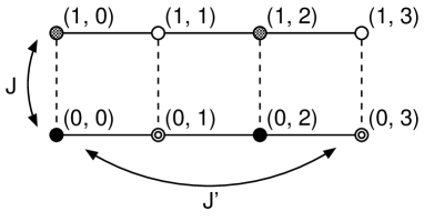
Figure 1: The graph for the regular NIM-rep of $SU(2)_{1}\times SU(2)_{3}$. Each vertex corresponds to the Cardy state. The dashed (solid) lines stand for the fusion with $(1,0)$ ($(0,1)$). The arrows show the action of the simple currents $J=(1,0),J^{\prime}=(0,3)$ on the Cardy states. Black, grey, circled and white vertices express $(\tilde{b}(J,1),\tilde{b}(1,J^{\prime}))=(1,1),(-1,1),(1,-1)$ and $(-1,-1)$, respectively. (see eq.(3.15b))

The group $H\subset G_{\mathrm{sc}}$ acts on $\psi$ as

$$\psi_{(J\alpha,J^{\prime}\beta)}{}^{(\mu,\nu)}=\psi_{(1-\alpha,3-\beta)}{}^{(\mu,\nu)}=\psi_{(\alpha,\beta)}{}^{(\mu,\nu)}(-1)^{\mu+\nu}.$$ (3.25)

Since there is no fixed point in this action, we can apply the method in Section 2.3.1 to obtain a new NIM-rep of the product theory. Namely, the formula (2.39) yields a NIM-rep (see Fig.2)

$$\tilde{\psi}_{[(0,\alpha)]}{}^{(\mu,\nu)}=\sqrt{2}\psi_{(0,\alpha)}{}^{(\mu,\nu)}=S^{(3)}_{\alpha\nu},\quad[(0,\alpha)]\in\tilde{\mathcal{V}},\,(\mu,\nu)\in\tilde{\mathcal{E}}.$$ (3.26)

Here the set $\tilde{\mathcal{V}}$ of the labels of the Cardy states and the set $\tilde{\mathcal{E}}$ of the labels of the Ishibashi states are given by

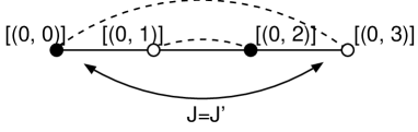
Figure 2: The simple current NIM-rep (3.26) of $SU(2)_{1}\times SU(2)_{3}$. The dashed (solid) lines stand for the fusion with $(1,0)$ ($(0,1)$). The arrows show the action of the simple currents $J=J^{\prime}$. Black (white) vertices express $\tilde{b}(J,J^{\prime})=1\,(-1)$.

$$\tilde{\mathcal{V}} =\{[(0,\alpha)]|\alpha=0,1,2,3\},$$ (3.27)

$$\tilde{\mathcal{E}} =\{(\mu,\nu)\in\mathcal{I}\,|\,(-1)^{\mu+\nu}=1\}=\{(0,0),(1,1),(0,2),(1,3)\}.$$ (3.28)

The action of the simple currents on the Cardy states has a non-trivial stabilizer

$$\mathcal{S}(\tilde{\mathcal{V}})=\{(1,1),(J,J^{\prime})\}=H\subset G_{\mathrm{sc}}.$$ (3.29)

The automorphism group $G(\tilde{\mathcal{V}})$ therefore reads

$$G(\tilde{\mathcal{V}})=G_{\mathrm{sc}}/\mathcal{S}(\tilde{\mathcal{V}})\cong\mathbb{Z}_{2}.$$ (3.30)

On the other hand, the automorphism group $G(\tilde{\mathcal{E}})$ takes the form

$$G(\tilde{\mathcal{E}})=\{(1,1),(J,J^{\prime})\}=H\cong\mathbb{Z}_{2}.$$ (3.31)

We show the action of these groups in Fig.2.

One can see that the diagonalization matrix (3.26) can not be factorized into the $SU(2)_{1}$ and the $SU(2)_{3}$ parts; the sets $\tilde{\mathcal{V}}$ and $\tilde{\mathcal{E}}$ are not of the factorized form. This NIM-rep corresponds to the $\mathbb{Z}_{2}$ orbifold of $SU(2)_{1}\times SU(2)_{3}$. Actually, the partition function of the orbifold can be obtained by the standard construction and takes the form

$$Z=\lvert\chi_{(0,0)}+\chi_{(1,3)}\rvert^{2}+\lvert\chi_{(1,1)}+\chi_{(0,2)}\rvert^{2}.$$ (3.32)

The spectrum of the orbifold matches to the set $\tilde{\mathcal{E}}$ obtained above.

3.3.2 NIM-rep from conformal embedding

$k$	$l$	$g$	$c$
1	3	$G_{2,1}$	$\frac{14}{5}$
2	2	$A_{3,1}$	$3$
3	8	$C_{3,1}$	$\frac{21}{5}$
2	10	$D_{4,1}$	$4$
6	6	$B_{4,1}$	$\frac{9}{2}$
8	28	$F_{4,1}$	$\frac{26}{5}$
10	10	$D_{5,1}$	$5$

Table 1: Conformal embeddings of $su(2)_{k}\oplus su(2)_{l}$ into an affine Lie algebra $g$. The subscript $1$ means that the level of the algebra is $1$. $c$ is the central charge of the embedding.

The method of conformal embedding also gives us non-trivial examples of the NIM-reps in tensor product theories. The possible embeddings for $su(2)_{k}\oplus su(2)_{l}$ is summarized in Table 1 [38]. Note that the level of the algebra $g$ is equal to $1$ for all the conformal embeddings. Among them, we consider the case of $k\neq l$. This is because, in the next section, we use the resulting NIM-rep in the construction of the NIM-rep of the diagonal coset theory $SU(2)_{l-k}\times SU(2)_{k}/SU(2)_{l}$. For the coset to be non-trivial, we need $k<l$. In the following, we consider two examples with $k\neq l$: $su(2)_{1}\oplus su(2)_{3}\subset G_{2,1}$ and $su(2)_{3}\oplus su(2)_{8}\subset C_{3,1}$.

$su(2)_{1}\oplus su(2)_{3}\subset G_{2,1}$

There are two integrable representations in $G_{2}$ at level $1$,

$$\mathcal{I}=P_{+}^{1}(G_{2})=\{(0,0),(0,1)\}.$$ (3.33)

In our convention, the short root is $\alpha_{2}$. The modular transformation $S$-matrix for $G_{2,1}$ reads

$$S=\frac{2}{\sqrt{5}}\begin{pmatrix}\sin\frac{\pi}{5}&\sin\frac{2\pi}{5}\\[6.0pt] \sin\frac{2\pi}{5}&-\sin\frac{\pi}{5}\end{pmatrix},$$ (3.34)

where the rows and columns are ordered as in eq.(3.33). These representations branch to those of $su(2)_{1}\oplus su(2)_{3}$ as follows,

$$\begin{array}[]{ll}h=0:&(0,0)\mapsto(0,0)\oplus(1,3),\\ h=\frac{2}{5}:&(0,1)\mapsto(1,1)\oplus(0,2).\end{array}$$ (3.35)

Here $h$ is the conformal dimension of the representation of $G_{2,1}$.

Let $|\alpha\rangle=\sum_{\mu\in\mathcal{I}}S_{\alpha\mu}|\mu\rangle\!\rangle\,(\alpha\in\{(0,0),(0,1)\})$ be the regular Cardy states of $G_{2,1}$. Using the branching rule (3.35) and the formula (2.46), we can regard these boundary states as those of the $SU(2)_{1}\times SU(2)_{3}$ theory. The spectrum of the Ishibashi states (see eq.(2.47)) can be read off from the branching rule,

$$\mathcal{E}_{(1,3)}=\{(0,0),(1,1),(0,2),(1,3)\}.$$ (3.36)

In terms of these states, the $G_{2,1}$ Cardy state can be written as a four-dimensional (row) vector $\psi_{\alpha}$ (see eq.(2.48))

$$\begin{pmatrix}\psi_{(0,0)}\\[6.0pt] \psi_{(0,1)}\end{pmatrix}=\sqrt{\frac{2}{5}}\begin{pmatrix}\sin\frac{\pi}{5}&\sin\frac{2\pi}{5}&\sin\frac{2\pi}{5}&\sin\frac{\pi}{5}\\[6.0pt] \sin\frac{2\pi}{5}&-\sin\frac{\pi}{5}&\sin-\frac{\pi}{5}&\sin\frac{2\pi}{5}\end{pmatrix},$$ (3.37)

where the columns are ordered as in eq.(3.36). Since $\lvert\mathcal{E}_{(1,3)}\rvert=4$, there are two states missing. We can obtain these two states by the boundary state generating technique in Section 2.3.2. (see also Appendix A.) The resulting boundary states are written as follows,

$$\begin{pmatrix}\psi_{0}=\psi_{(0,0)}\\[6.0pt] \psi_{1}\\[6.0pt] \psi_{2}=\psi_{(0,1)}\\[6.0pt] \psi_{3}\end{pmatrix}=\sqrt{\frac{2}{5}}\begin{pmatrix}\sin\frac{\pi}{5}&\sin\frac{2\pi}{5}&\sin\frac{2\pi}{5}&\sin\frac{\pi}{5}\\[6.0pt] \sin\frac{2\pi}{5}&\sin\frac{\pi}{5}&-\sin\frac{\pi}{5}&-\sin\frac{2\pi}{5}\\[6.0pt] \sin\frac{2\pi}{5}&-\sin\frac{\pi}{5}&-\sin\frac{\pi}{5}&\sin\frac{2\pi}{5}\\[6.0pt] \sin\frac{\pi}{5}&-\sin\frac{2\pi}{5}&\sin\frac{2\pi}{5}&-\sin\frac{\pi}{5}\end{pmatrix}.$$ (3.38)

We obtain four Cardy states from the conformal embedding $su(2)_{1}\oplus su(2)_{3}\subset G_{2,1}$. As is seen from eq.(3.36), this NIM-rep is not factorizable.

The spectrum (3.36) is the same as that for the simple current NIM-rep (3.28). Actually, the NIM-rep obtained above is nothing but that obtained from the simple current. This is no coincidence. The partition function obtained from the affine branching rule (3.35) reads

$$Z=\lvert\chi^{G_{2}}_{(0,0)}\rvert^{2}+\lvert\chi^{G_{2}}_{(0,1)}\rvert^{2}=\lvert\chi_{(0,0)}+\chi_{(1,3)}\rvert^{2}+\lvert\chi_{(1,1)}+\chi_{(0,2)}\rvert^{2},$$ (3.39)

which is exactly that for the orbifold (3.32).

$su(2)_{3}\oplus su(2)_{8}\subset C_{3,1}$

The construction for the case of $su(2)_{3}\oplus su(2)_{8}\subset C_{3,1}$ proceeds exactly the same way as above. There are four integrable representations in $C_{3}$ at level $1$,

$$\mathcal{I}=P_{+}^{1}(C_{3})=\{(0,0,0),(1,0,0),(0,1,0),(0,0,1)\}.$$ (3.40)

In our convention, the long root is $\alpha_{3}$. The modular transformation $S$-matrix for $C_{3}$ at level $1$ is given by that for $su(2)_{3}$,

$$S=\sqrt{\frac{2}{5}}\begin{pmatrix}\sin\frac{\pi}{5}&\sin\frac{2\pi}{5}&\sin\frac{2\pi}{5}&\sin\frac{\pi}{5}\\[6.0pt] \sin\frac{2\pi}{5}&\sin\frac{\pi}{5}&-\sin\frac{\pi}{5}&-\sin\frac{2\pi}{5}\\[6.0pt] \sin\frac{2\pi}{5}&-\sin\frac{\pi}{5}&-\sin\frac{\pi}{5}&\sin\frac{2\pi}{5}\\[6.0pt] \sin\frac{\pi}{5}&-\sin\frac{2\pi}{5}&\sin\frac{2\pi}{5}&-\sin\frac{\pi}{5}\end{pmatrix},$$ (3.41)

where the rows and columns are ordered as in eq.(3.40). The branching rule (2.44) is found by comparing the conformal dimension,

$$\left.\begin{array}[]{lcl}h=0&:&(0,0,0)\mapsto(0,0)\oplus(2,4)\oplus(0,8),\\ h=\frac{7}{20}&:&(1,0,0)\mapsto(1,2)\oplus(3,4)\oplus(1,6),\\ h=\frac{3}{5}&:&(0,1,0)\mapsto(2,2)\oplus(0,4)\oplus(2,6),\\ h=\frac{3}{4}&:&(0,0,1)\mapsto(3,0)\oplus(1,4)\oplus(3,8),\end{array}\right.$$ (3.42)

where $(\mu,\nu)$ in the r.h.s. is the representation of the $SU(2)_{3}\times SU(2)_{8}$ theory. $h$ is the conformal dimension of the representation of $C_{3,1}$.

From (3.42), one obtains the set of Ishibashi states (2.47)

$$\begin{split}\mathcal{E}_{(3,8)}=\{&(0,0),(3,0),(2,2),(1,2),(2,6),(1,6),\\ &(0,8),(3,8),(0,4),(3,4),(2,4),(1,4)\}.\end{split}$$ (3.43)

The formula (2.46) gives four boundary states labeled by $(\lambda_{1},\lambda_{2},\lambda_{3})\in\mathcal{I}$. Since $\lvert\mathcal{E}_{(3,8)}\rvert=12$, there are eight states missing. The boundary states generating technique again enables us to construct them. The missing states are generated from four regular Cardy states of $C_{3,1}$ by taking the fusion with $(1,0)$ and $(0,1)$. We show the result in Fig.3. One can see that twelve states are organized in two different ways: three sets of four states connected by $(1,0)$ and two sets of six states by $(0,1)$. The states connected by $(1,0)$ realize the regular NIM-rep of $su(2)_{3}$, while those connected by $(0,1)$ are two copies of the $D_{6}$ NIM-rep of $su(2)_{8}$. The resulting NIM-rep is not of the factorized form, rather two kinds of diagrams are folded into one graph (cf Fig.1).

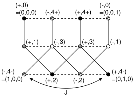
Figure 3: The NIM-rep graph of the $SU(2)_{3}\times SU(2)_{8}$ theory from the conformal embedding $su(2)_{3}\oplus su(2)_{8}\subset C_{3,1}$. The dashed (solid) lines stand for the fusion with $(1,0)\,((0,1))$. The arrow shows the action of the simple currents $J=(3,0)$ on the Cardy states. $J^{\prime}=(0,8)$ belongs to the stabilizer. Black, circled, grey and white vertices express $(\tilde{b}(J,1),\tilde{b}(1,J^{\prime}))=(1,1),(-1,1),(1,-1)$ and $(-1,-1)$, respectively. The vertices connected by a dashed (solid) line form a $A_{4}$ ($D_{6}$) Dynkin diagram.

It is therefore natural to introduce the label $(\pm,i)$, $i=0,1,2,3,4_{\pm},$ for the boundary states

$$\begin{split}\mathcal{V}_{(3,8)}=\{&(+,0),(-,0),(+,1),(-,1),(+,2),(-,2),\\ &(+,3),(-,3),(+,4_{+}),(-,4_{+}),(+,4_{-}),(-,4_{-})\}.\end{split}$$ (3.44)

The first entry distinguishes two copies of $D_{6}$. The sign $\pm$ stands for the eigenvalue $\tilde{b}(J,1)$. The second entry labels the vertices of $D_{6}$; $0$ for the end point of the long leg and $4_{\pm}$ for two short legs. In this labeling, the regular Cardy states $\{(0,0,0),(1,0,0),(0,1,0),(0,0,1)\}$ of $C_{3,1}$ correspond to $\{(+,0),(-,4_{-}),(+,4_{-}),(-,0)\}$, respectively.

The action of the simple currents on the Cardy states has a non-trivial stabilizer

$$\mathcal{S}(\mathcal{V})=\{(1,1),(1,J^{\prime})\}\subset G_{\mathrm{sc}}.$$ (3.45)

The automorphism group $G(\mathcal{V})$ therefore reads

$$G(\mathcal{V})=G_{\mathrm{sc}}/\mathcal{S}(\mathcal{V})=\{(1,1),(J,1)\}\cong\mathbb{Z}_{2},$$ (3.46)

while the automorphism group $G(\mathcal{E})$ is $G_{\mathrm{sc}}$ itself. We show the action of these groups in Fig.3.

We give the explicit form of the diagonalization matrix $\psi^{(3,8)}{}_{\alpha}{}^{(\mu,\nu)}$,

$$\psi^{(3,8)}=\frac{1}{\sqrt{5}}\begin{pmatrix}\sqrt{2}c_{2}K&\sqrt{2}c_{1}K&\sqrt{2}c_{1}K&\sqrt{2}c_{2}K&K&K\\[3.0pt] \sqrt{2}s_{1}K&\sqrt{2}s_{2}K&-\sqrt{2}s_{2}K&-\sqrt{2}s_{1}K&0&0\\[3.0pt] \sqrt{2}c_{1}K&\sqrt{2}c_{2}K&\sqrt{2}c_{2}K&\sqrt{2}c_{1}K&-K&-K\\[3.0pt] \sqrt{2}s_{2}K&-\sqrt{2}s_{1}K&\sqrt{2}s_{1}K&-\sqrt{2}s_{2}K&0&0\\[3.0pt] \frac{1}{\sqrt{2}}K&-\frac{1}{\sqrt{2}}K&-\frac{1}{\sqrt{2}}K&\frac{1}{\sqrt{2}}K&2c_{1}K&-2c_{2}K\\[3.0pt] \frac{1}{\sqrt{2}}K&-\frac{1}{\sqrt{2}}K&-\frac{1}{\sqrt{2}}K&\frac{1}{\sqrt{2}}K&-2c_{2}K&2c_{1}K\end{pmatrix},$$ (3.47a)

where

$$\begin{split}&K=\frac{1}{\sqrt{2}}\begin{pmatrix}1&1\\ 1&-1\end{pmatrix},\\ &c_{1}=\cos\frac{\pi}{5},\quad c_{2}=\cos\frac{2\pi}{5},\quad s_{1}=\sin\frac{\pi}{5},\quad s_{2}=\sin\frac{2\pi}{5}.\end{split}$$ (3.47b)

The rows $\alpha$ are ordered as in eq.(3.44) whereas the columns $(\mu,\nu)$ are ordered as in eq.(3.43).

4 Boundary states in coset theories

In this section, we develop a method to construct NIM-reps in coset conformal field theories. Our strategy is to use the relation of the $G/H$ theory with the tensor product theory $G\times H^{c}$ [24]. Namely, we give a prescription to construct NIM-reps of coset theories from those of tensor product theories, which are discussed in the last section. As an example, we apply our method to the $SU(2)_{5}\times SU(2)_{3}/SU(2)_{8}$ theory to obtain a NIM-rep which is not factorizable into the $SU(2)_{5}\times SU(2)_{3}$ and $SU(2)_{8}$ parts.

4.1 $G/H$ theories

The $G/H$ theory is based on an embedding of the affine Lie algebra $h$ into $g$. A representation $\mu$ of $g$ is decomposed by representations $\nu$ of $h$ as follows,

$$\mu=\operatorname*{\oplus}_{\nu}(\mu;\nu)\nu.$$ (4.1)

The spectrum $\hat{\mathcal{I}}$ of the $G/H$ theory consists of all the possible combination $(\mu;\nu)$,

$$\begin{split}\hat{\mathcal{I}}=\{(\mu;\nu)|\,&\mu\in\mathcal{I}^{G},\nu\in\mathcal{I}^{H},\\ &b^{G}_{\mu}(J)=b^{H}_{\nu}(J^{\prime}),(J\mu;J^{\prime}\nu)=(\mu;\nu),\forall(J,J^{\prime})\in G_{\mathrm{id}}\}.\end{split}$$ (4.2)

Here $\mathcal{I}^{G}$ $(\mathcal{I}^{H})$ is the spectrum of the $G$ $(H)$ theory. $G_{\mathrm{id}}$ is the group of the identification currents corresponding to the common center of $G$ and $H$. $b^{G}_{\mu}(J)$ ($b^{H}_{\nu}(J^{\prime})$) expresses the monodromy charge of the $G$ ($H$) theory. The condition $b^{G}_{\mu}(J)=b^{H}_{\nu}(J^{\prime})$ is the selection rule of the branching of representations, while the relation $(J\mu;J^{\prime}\nu)=(\mu;\nu)$ is the so-called field identification.In this paper, we restrict ourselves to the case that all the identification orbit have the same length $N_{0}=\lvert G_{\mathrm{id}}\rvert$,

$$N_{0}=\lvert\{(J\mu,J^{\prime}\nu)\in\mathcal{I}^{G}\otimes\mathcal{I}^{H}|\,(J,J^{\prime})\in G_{\mathrm{id}}\}\rvert=\lvert G_{\mathrm{id}}\rvert.$$ (4.3)

In particular, there is no fixed point in the field identification [39]

$$(J\mu,J^{\prime}\nu)\neq(\mu,\nu),\quad\forall(\mu,\nu)\in\mathcal{I}^{G}\otimes\mathcal{I}^{H},\quad\forall(J,J^{\prime})\neq 1\in G_{\mathrm{id}}.$$ (4.4)

The character of the coset theory is the branching function $\chi_{(\mu;\nu)}$ of the algebra embedding $h\subset g$. From the branching rule (4.1), we find

$$\chi_{\mu}^{G}=\sum_{\nu}\chi_{(\mu;\nu)}\chi_{\nu}^{H}.$$ (4.5)

The modular transformation $S$-matrix of the $G/H$ theory reads

$$\hat{S}_{(\mu;\nu)(\mu^{\prime};\nu^{\prime})}=N_{0}S_{\mu\mu^{\prime}}^{G}\overline{{S_{\nu\nu^{\prime}}^{H}}}=N_{0}S_{\mu\mu^{\prime}}^{G}S^{H}_{\nu\bar{\nu^{\prime}}},$$ (4.6)

where $N_{0}$ is the length of the identification orbit (4.3) and $S^{G}$ ($S^{H}$) is the $S$-matrix of the $G$ ($H$) theory.

As is seen from the form of the $S$-matrix (4.6), it is natural to relate the $G/H$ theory with the tensor product theory $G\times H^{c}$. Here $H^{c}$ stands for a theory whose spectrum and $S$-matrix are given by $\mathcal{I}^{H}$ and $\overline{S^{H}}$, respectively. The spectrum $\mathcal{I}^{c}$ and the $S$-matrix $S^{c}$ of the $G\times H^{c}$ theory are therefore given by

$$\mathcal{I}^{c}=\mathcal{I}^{G\times H^{c}}=\mathcal{I}^{G}\otimes\mathcal{I}^{H}=\mathcal{I}^{G\times H}\equiv\mathcal{I},$$ (4.7)

$$S^{c}_{(\mu,\nu)(\mu^{\prime},\nu^{\prime})}=S^{G}_{\mu\mu^{\prime}}\overline{S^{H}_{\nu\nu^{\prime}}}=S^{G}_{\mu\mu^{\prime}}S^{H}_{\nu\bar{\nu^{\prime}}}\equiv S_{(\mu,\nu)(\mu^{\prime},\bar{\nu^{\prime}})},$$ (4.8)

where we denote by $\mathcal{I}$ and $S$ the spectrum and the $S$-matrix of the $G\times H$ theory, respectively. The fusion algebra of the $G\times H^{c}$ theory is the same as that of the $G\times H$ theory. From the Verlinde formula (2.12), one can calculate the fusion coefficients,

$$\begin{split}\mathcal{N}^{c}_{(\mu,\nu)(\mu^{\prime},\nu^{\prime})}{}^{(\mu^{\prime\prime},\nu^{\prime\prime})}&=\sum_{(\rho,\sigma)\in\mathcal{I}}\frac{S^{c}_{(\mu,\nu)(\rho,\sigma)}S^{c}_{(\mu^{\prime},\nu^{\prime})(\rho,\sigma)}\overline{S^{c}_{(\mu^{\prime\prime},\nu^{\prime\prime})(\rho,\sigma)}}}{S^{c}_{(0,0)(\rho,\sigma)}}\\ &=\sum_{(\rho,\bar{\sigma})\in\mathcal{I}}\frac{S_{(\mu,\nu)(\rho,\bar{\sigma})}S_{(\mu^{\prime},\nu^{\prime})(\rho,\bar{\sigma})}\overline{S_{(\mu^{\prime\prime},\nu^{\prime\prime})(\rho,\bar{\sigma})}}}{S_{(0,0)(\rho,\bar{\sigma})}}\\ &=\mathcal{N}_{(\mu,\nu)(\mu^{\prime},\nu^{\prime})}{}^{(\mu^{\prime\prime},\nu^{\prime\prime})}.\end{split}$$ (4.9)

The simple current group of the $G\times H^{c}$ theory is therefore the same as that of the $G\times H$ theory, which we denote by $G_{\mathrm{sc}}\equiv G_{\mathrm{sc}}^{G\times H}$. The action of the simple current group $G_{\mathrm{sc}}$ on the $S$-matrix reads

$$\begin{split}S_{(J\mu,J^{\prime}\nu)(\mu^{\prime},\nu^{\prime})}&=S_{(\mu,\nu)(\mu^{\prime},\nu^{\prime})}b_{(\mu^{\prime},\nu^{\prime})}(J,J^{\prime}),\\ S^{c}_{(J\mu,J^{\prime}\nu)(\mu^{\prime},\nu^{\prime})}&=S^{c}_{(\mu,\nu)(\mu^{\prime},\nu^{\prime})}b^{c}_{(\mu^{\prime},\nu^{\prime})}(J,J^{\prime}),\quad(J,J^{\prime})\in G_{\mathrm{sc}},\end{split}$$ (4.10)

where $b$ and $b^{c}$ are defined as

$$\begin{split}b_{(\mu,\nu)}(J,J^{\prime})&=b^{G}_{\mu}(J)b^{H}_{\nu}(J^{\prime}),\\ b^{c}_{(\mu,\nu)}(J,J^{\prime})&=b_{(\mu,\bar{\nu})}(J,J^{\prime})=b^{G}_{\mu}(J)\overline{b^{H}_{\nu}(J^{\prime})},\quad(J,J^{\prime})\in G_{\mathrm{sc}}.\end{split}$$ (4.11)

In terms of the $G\times H^{c}$ theory, the identification current group $G_{\mathrm{id}}$ is a subgroup of the simple current group $G_{\mathrm{sc}}$. The field identification $(J\mu;J^{\prime}\nu)=(\mu;\nu),(J,J^{\prime})\in G_{\mathrm{id}},$ therefore corresponds to taking the quotient of $\mathcal{I}$ by $G_{\mathrm{id}}$, and the selection rule $b^{G}_{\mu}(J)=b^{H}_{\nu}(J^{\prime}),(J,J^{\prime})\in G_{\mathrm{id}},$ is the condition of the vanishing monodromy charge $b^{c}_{(\mu,\nu)}=1$ with respect to $G_{\mathrm{id}}$. Hence the definition (4.2) of the spectrum can be rewritten as follows,

$$\begin{split}\hat{\mathcal{I}}=\{(\mu;\nu)|\,&(\mu,\nu)\in\mathcal{I},\\ &b^{c}_{(\mu,\nu)}(J)=1,J(\mu,\nu)\sim(\mu,\nu),\forall J\in G_{\mathrm{id}}\}.\end{split}$$ (4.12)

From now on, we denote the simple current of the tensor product theory by a single letter such as $J$ instead of a pair of letters $(J,J^{\prime})$. The $S$-matrix (4.6) is also expressed as

$$\hat{S}_{(\mu;\nu)(\mu^{\prime};\nu^{\prime})}=N_{0}S^{c}_{(\mu,\nu)(\mu^{\prime},\nu^{\prime})}.$$ (4.13)

This definition of the $S$-matrix $\hat{S}$ has to be consistent with the field identification. This is assured by the selection rule,

$$S^{c}_{J(\mu,\nu)(\mu^{\prime},\nu^{\prime})}=S^{c}_{(\mu,\nu)(\mu^{\prime},\nu^{\prime})}b^{c}_{(\mu^{\prime},\nu^{\prime})}(J)=S^{c}_{(\mu,\nu)(\mu^{\prime},\nu^{\prime})},\quad J\in G_{\mathrm{id}}\quad(b^{c}_{(\mu^{\prime},\nu^{\prime})}(J)=1).$$ (4.14)

Here we used the property (4.10). Next, most importantly, $\hat{S}$ should be unitary,

$$\begin{split}\sum_{(\mu^{\prime};\nu^{\prime})\in\hat{\mathcal{I}}}\hat{S}_{(\mu;\nu)(\mu^{\prime};\nu^{\prime})}\overline{\hat{S}_{(\mu^{\prime\prime};\nu^{\prime\prime})(\mu^{\prime};\nu^{\prime})}}&=\sum_{(\mu^{\prime};\nu^{\prime})\in\hat{\mathcal{I}}}N_{0}^{2}S^{c}_{(\mu,\nu)(\mu^{\prime},\nu^{\prime})}\overline{S^{c}_{(\mu^{\prime\prime},\nu^{\prime\prime})(\mu^{\prime},\nu^{\prime})}}\\ &=\frac{1}{N_{0}}\sum_{(\mu^{\prime},\nu^{\prime})\in\mathcal{I}}\frac{1}{N_{0}}\sum_{J\in G_{\mathrm{id}}}b^{c}_{(\mu^{\prime},\nu^{\prime})}(J)\,\\ &\quad\quad\quad\quad\times N_{0}^{2}S^{c}_{(\mu,\nu)(\mu^{\prime},\nu^{\prime})}\overline{S^{c}_{(\mu^{\prime\prime},\nu^{\prime\prime})(\mu^{\prime},\nu^{\prime})}}\\ &=\sum_{J\in G_{\mathrm{id}}}\sum_{(\mu^{\prime},\nu^{\prime})\in\mathcal{I}}S^{c}_{J(\mu,\nu)(\mu^{\prime},\nu^{\prime})}\overline{S^{c}_{(\mu^{\prime\prime},\nu^{\prime\prime})(\mu^{\prime},\nu^{\prime})}}\\ &=\sum_{J\in G_{\mathrm{id}}}\delta_{J(\mu,\nu)(\mu^{\prime\prime},\nu^{\prime\prime})}\\ &=\delta_{(\mu;\nu)(\mu^{\prime\prime};\nu^{\prime\prime})}.\end{split}$$ (4.15)

Here we used our assumption of no fixed points to rewrite the sum

$$\sum_{(\mu^{\prime};\nu^{\prime})\in\hat{\mathcal{I}}}\rightarrow\quad\frac{1}{N_{0}}\sum_{(\mu^{\prime},\nu^{\prime})\in\mathcal{I}}\frac{1}{N_{0}}\sum_{J\in G_{\mathrm{id}}}b^{c}_{(\mu^{\prime},\nu^{\prime})}(J).$$ (4.16)

The projection operator introduced above takes account of the selection rule.

The fusion coefficients of the coset theory can be calculated via the Verlinde formula (2.12),

$$\begin{split}\hat{\mathcal{N}}_{(\mu;\nu)(\mu^{\prime};\nu^{\prime})}{}^{(\mu^{\prime\prime};\nu^{\prime\prime})}&=\sum_{(\rho;\sigma)\in\hat{\mathcal{I}}}\frac{\hat{S}_{(\mu;\nu)(\rho;\sigma)}\hat{S}_{(\mu^{\prime};\nu^{\prime})(\rho;\sigma)}\overline{\hat{S}_{(\mu^{\prime\prime};\nu^{\prime\prime})(\rho;\sigma)}}}{\hat{S}_{(0;0)(\rho;\sigma)}}\\ &=\frac{1}{N_{0}}\sum_{(\rho,\sigma)\in\mathcal{I}}\frac{1}{N_{0}}\sum_{J\in G_{\mathrm{id}}}b^{c}_{(\rho,\sigma)}(J)\times N_{0}^{2}\frac{S^{c}_{(\mu,\nu)(\rho,\sigma)}S^{c}_{(\mu^{\prime},\nu^{\prime})(\rho,\sigma)}\overline{S^{c}_{(\mu^{\prime\prime},\nu^{\prime\prime})(\rho,\sigma)}}}{S^{c}_{(0,0)(\rho,\sigma)}}\\ &=\sum_{J\in G_{\mathrm{id}}}\mathcal{N}_{(\mu,\nu)\,J(\mu^{\prime},\nu^{\prime})}{}^{(\mu^{\prime\prime},\nu^{\prime\prime})}.\end{split}$$ (4.17)

Here we used the fact (4.9) that the fusion rule of the $G\times H^{c}$ theory is the same as that of the $G\times H$ theory.

4.2 NIM-reps in coset theories

Since the $G/H$ theory is related to the $G\times H^{c}$ theory, it is natural to expect that NIM-reps in the $G/H$ theory is related to NIM-reps in the $G\times H^{c}$ theory. In [18], it was shown that a NIM-rep $\hat{\psi}$ in the $G/H$ theory can be constructed as a product of NIM-reps in the $G$ theory ($\psi^{G}$) and the $H$ theory ($\psi^{H}$),

$$\hat{\psi}\sim\psi^{G}\overline{\psi^{H}}.$$ (4.18)

Since $\overline{\psi^{H}}$ is a NIM-rep of the $H^{c}$ theory, the above relation is considered to be a map from NIM-reps of the $G\times H^{c}$ theory to those of the $G/H$ theory.

In this subsection, we extend the construction in [18] to more general class of NIM-reps. Namely, we give a map from NIM-reps of the $G\times H^{c}$ theory to those of the $G/H$ theory, without the assumption that NIM-reps in the $G\times H^{c}$ theory are factorizable into the $G$ and $H^{c}$ theories as in eq.(4.18). The problem is to find a map from a given NIM-rep (3.14) in the $G\times H^{c}$ theory to a NIM-rep in the $G/H$ theory

$$(\hat{n}_{(\mu;\nu)})_{[\alpha]}{}^{[\beta]}=\sum_{(\mu^{\prime};\nu^{\prime})\in\hat{\mathcal{E}}}\hat{\psi}_{[\alpha]}{}^{(\mu^{\prime};\nu^{\prime})}\frac{\hat{S}_{(\mu;\nu)(\mu^{\prime};\nu^{\prime})}}{\hat{S}_{(0;0)(\mu^{\prime};\nu^{\prime})}}\overline{\hat{\psi}_{[\beta]}{}^{(\mu^{\prime};\nu^{\prime})}},\quad[\alpha],[\beta]\in\hat{\mathcal{V}},$$ (4.19)

with an appropriate choice of the sets $\hat{\mathcal{V}}$ of the labels of the Cardy states and $\hat{\mathcal{E}}$ of the Ishibashi states.

The prototype of our map is eq.(4.13), which relates the $S$-matrices (i.e., the regular NIM-reps) of the $G\times H^{c}$ and $G/H$ theories. This relation suggests that a NIM-rep of the $G/H$ theory can be written in the form

$$\hat{\psi}_{[\alpha]}{}^{(\mu;\nu)}=N\psi^{c}_{\alpha}{}^{(\mu,\nu)}.\quad$$ (4.20)

Here $\psi^{c}$ is the diagonalization matrix of a NIM-rep of the $G\times H^{c}$ theory, and $N$ is an appropriate constant. The label $[\alpha]$ of the boundary states will be defined shortly.

In order to use the above expression (4.20), we need a NIM-rep $\psi^{c}$ of the $G\times H^{c}$ theory. As is shown below, we can construct $\psi^{c}$ from a NIM-rep of the $G\times H$ theory. Suppose that $\psi$ gives a NIM-rep of the $G\times H$ theory as in eq.(3.14). Then one can show that the following matrix yields a NIM-rep of the $G\times H^{c}$ theory,

$$\psi^{c}_{\alpha}{}^{(\mu,\nu)}=\psi_{\alpha}{}^{(\mu,\bar{\nu})},\quad\alpha\in\mathcal{V}^{c}=\mathcal{V},\quad(\mu,\nu)\in\mathcal{E}^{c}.$$ (4.21)

Here we introduced the set $\mathcal{E}^{c}$ of the Ishibashi states for $\psi^{c}$, which is determined from $\mathcal{E}$ by taking the charge conjugation only in the $H$ sector,

$$\mathcal{E}^{c}=\{(\mu,\nu)|(\mu,\bar{\nu})\in\mathcal{E}\}.$$ (4.22)

In general, $\mathcal{E}^{c}\neq\mathcal{E}$, since $(\mu,\nu)\mapsto(\mu,\bar{\nu})$ is not the charge conjugation of the entire theory. See Appendix B for an example of $\mathcal{E}^{c}\neq\mathcal{E}$. One can confirm that $\psi^{c}$ gives a NIM-rep of the $G\times H^{c}$ theory as follows,

$$\begin{split}(n^{c}_{(\mu,\nu)})_{\alpha}{}^{\beta}&=\sum_{(\mu^{\prime},\nu^{\prime})\in\mathcal{E}^{c}}\psi^{c}_{\alpha}{}^{(\mu^{\prime},\nu^{\prime})}\frac{S^{c}_{(\mu,\nu)(\mu^{\prime},\nu^{\prime})}}{S^{c}_{(0,0)(\mu^{\prime},\nu^{\prime})}}\overline{\psi^{c}_{\beta}{}^{(\mu^{\prime},\nu^{\prime})}}\\ &=\sum_{(\mu^{\prime},\nu^{\prime})\in\mathcal{E}^{c}}\psi_{\alpha}{}^{(\mu^{\prime},\bar{\nu^{\prime}})}\frac{S_{(\mu,\nu)(\mu^{\prime},\bar{\nu^{\prime}})}}{S_{(0,0)(\mu^{\prime},\bar{\nu^{\prime}})}}\overline{\psi_{\beta}{}^{(\mu^{\prime},\bar{\nu^{\prime}})}}\\ &=\sum_{(\mu^{\prime},\nu^{\prime})\in\mathcal{E}}\psi_{\alpha}{}^{(\mu^{\prime},\nu^{\prime})}\frac{S_{(\mu,\nu)(\mu^{\prime},\nu^{\prime})}}{S_{(0,0)(\mu^{\prime},\nu^{\prime})}}\overline{\psi_{\beta}{}^{(\mu^{\prime},\nu^{\prime})}}\\ &=(n_{(\mu,\nu)})_{\alpha}{}^{\beta}\quad(\alpha,\beta\in\mathcal{V}),\end{split}$$ (4.23)

where we used eq.(3.14). Hence $\psi^{c}$ in eq.(4.21) gives the same NIM-rep as that for the original $G\times H$ theory. The special case of the map (4.21) is the relation (4.8) of the $S$-matrices $S^{c}$ and $S$, for which $\mathcal{E}^{c}=\mathcal{I}^{c}=\mathcal{I}$.

We need the action of the simple currents on $\psi^{c}$. The action of the simple currents $J\in G_{\mathrm{sc}}$ on $\psi$ reads (see eq.(3.15))

$$\psi_{J\alpha}{}^{(\mu,\nu)} =\psi_{\alpha}{}^{(\mu,\nu)}b_{(\mu,\nu)}(J), J\in G(\mathcal{V}),$$ (4.24a)

$${\psi_{\alpha}}^{J(\mu,\nu)} =\tilde{b}_{\alpha}(J){\psi_{\alpha}}^{(\mu,\nu)}, J\in G(\mathcal{E}),$$ (4.24b)

where $b_{(\mu,\nu)}(J)$ is defined in eq.(4.11). From this equation and the definition (4.21) of $\psi^{c}$, the action on $\psi^{c}$ follows immediately,

$${\psi^{c}_{J\alpha}}^{(\mu,\nu)} ={\psi^{c}_{\alpha}}^{(\mu,\nu)}b^{c}_{(\mu,\nu)}(J), J\in G(\mathcal{V}^{c}),$$ (4.25a)

$${\psi^{c}_{\alpha}}^{J(\mu,\nu)} =\tilde{b}^{c}_{\alpha}(J){\psi^{c}_{\alpha}}^{(\mu,\nu)}, J\in G(\mathcal{E}^{c}),$$ (4.25b)

where $b^{c}_{(\mu,\nu)}(J)$ is also defined in eq.(4.11). We introduced two groups, $G(\mathcal{V}^{c})$ and $G(\mathcal{E}^{c})$. $G(\mathcal{E}^{c})$ is the automorphism group of $\mathcal{E}^{c}$,

$$G(\mathcal{E}^{c})=\{J\in G_{\mathrm{sc}}\,|\,J:\,\mathcal{E}^{c}\rightarrow\mathcal{E}^{c}\},$$ (4.26)

which is in general distinct from $G(\mathcal{E})$ since $\mathcal{E}^{c}\neq\mathcal{E}$. The charge $\tilde{b}^{c}_{\alpha}$ is defined so that the above equations, (4.24b) and (4.25b), are consistent with each other. $G(\mathcal{V}^{c})$ needs some explanation. As is seen from the definition (4.21) of $\psi^{c}$, the set of the labels of the Cardy states for $\psi^{c}$ is the same as that for $\psi$, i.e., $\mathcal{V}^{c}=\mathcal{V}$. However, the action of the simple currents on $\mathcal{V}^{c}$ differs from that on $\mathcal{V}$, namely $b^{c}(J)\neq b(J)$. We therefore introduce the stabilizer for $\mathcal{V}^{c}$ with respect to the action (4.25a), which we denote by $\mathcal{S}^{c}(\mathcal{V}^{c})$,

$$\mathcal{S}^{c}(\mathcal{V}^{c})=\{J\in G_{\mathrm{sc}}|\,b^{c}_{(\mu,\nu)}(J)=1\,\,\forall(\mu,\nu)\in\mathcal{E}^{c}\}.$$ (4.27)

The automorphism group $G(\mathcal{V}^{c})$ is defined as the quotient of $G_{\mathrm{sc}}$ by this stabilizer,

$$G(\mathcal{V}^{c})=G_{\mathrm{sc}}/\mathcal{S}^{c}(\mathcal{V}^{c}).$$ (4.28)

We return to eq.(4.20) and show that $\hat{\psi}$ gives a NIM-rep of the coset theory. We first specify the set $\hat{\mathcal{E}}$ of the labels of the Ishibashi states for $\hat{\psi}$. From the definition (4.20) of $\hat{\psi}$, one can read off $\hat{\mathcal{E}}$ in the form

$$\begin{split}\hat{\mathcal{E}}&=\{(\mu;\nu)\in\hat{\mathcal{I}}|\,(\mu,\nu)\in\mathcal{E}^{c}\}\\ &=\{(\mu;\nu)|(\mu,\nu)\in\mathcal{E}^{c},\,b^{c}_{(\mu,\nu)}(J)=1\,(\forall J\in G_{\mathrm{id}}),J(\mu,\nu)\sim(\mu,\nu)\,(\forall J\in G_{\mathrm{id}})\}.\end{split}$$ (4.29)

This expression for $\hat{\mathcal{E}}$ however contains some redundancies. First, the selection rule $b^{c}_{(\mu,\nu)}(J)=1\,(\forall J\in G_{\mathrm{id}})$ has some trivial equations if $G_{\mathrm{id}}$ has elements common with the stabilizer $\mathcal{S}^{c}(\mathcal{V}^{c})$ (see eq.(4.27)). The selection rules with respect to $J\in G_{\mathrm{id}}\cap\mathcal{S}^{c}(\mathcal{V}^{c})$ are trivially satisfied for $(\mu,\nu)\in\mathcal{E}^{c}$. The non-trivial selection rules are therefore obtained by considering the quotient group

$$G_{\mathrm{id}}(\mathcal{V}^{c})=G_{\mathrm{id}}/(G_{\mathrm{id}}\cap\mathcal{S}^{c}(\mathcal{V}^{c}))\subset G(\mathcal{V}^{c}).$$ (4.30)

The second redundancy in eq.(4.29) arises in the field identification. The spectrum $\mathcal{E}^{c}$ of the Ishibashi states differs from the spectrum $\mathcal{I}$ of the $G\times H^{c}$ theory, and the action of the identification currents $G_{\mathrm{id}}$ may not close on $\mathcal{E}^{c}$. We are therefore naturally led to the notion of the group of the field identifications restricted on $\mathcal{E}^{c}$,

$$G_{\mathrm{id}}(\mathcal{E}^{c})=\{J\in G_{\mathrm{id}}|\,J:\mathcal{E}^{c}\rightarrow\mathcal{E}^{c}\}=G_{\mathrm{id}}\cap G(\mathcal{E}^{c})\subset G(\mathcal{E}^{c}).$$ (4.31)

With these groups, we can rewrite the expression (4.29) in the form

$$\begin{split}\hat{\mathcal{E}}=\{(\mu;\nu)|(\mu,\nu)\in\mathcal{E}^{c},\,&b^{c}_{(\mu,\nu)}(J)=1\,(\forall J\in G_{\mathrm{id}}(\mathcal{V}^{c})),\\ &J(\mu,\nu)\sim(\mu,\nu)\,(\forall J\in G_{\mathrm{id}}(\mathcal{E}^{c}))\}.\end{split}$$ (4.32)

We turn to the set $\hat{\mathcal{V}}$ of the labels of the Cardy states in the coset theory. For $\hat{\psi}$ to be well-defined, eq.(4.20) should be consistent with the field identification. Since the field identification on $\mathcal{E}^{c}$ is described by the group $G_{\mathrm{id}}(\mathcal{E}^{c})$, the consistency condition can be written as

$$\psi^{c}_{\alpha}{}^{J(\mu,\nu)}=\tilde{b}^{c}_{\alpha}(J)\psi^{c}_{\alpha}{}^{(\mu,\nu)}=\psi^{c}_{\alpha}{}^{(\mu,\nu)},\quad\forall J\in G_{\mathrm{id}}(\mathcal{E}^{c}),$$ (4.33)

where we used eq.(4.25b). Hence, the consistency with the field identification requires the selection rule $\tilde{b}^{c}=1$ for the boundary states. We call this condition the brane selection rule [18]. We can consider the brane selection rule on $\mathcal{V}^{c}$ as the ‘dual’ of the field identification on $\mathcal{E}^{c}$. In order to obtain the spectrum $\hat{\mathcal{E}}$ of the coset theory from that of the tensor product, we have to impose one more projection, i.e., the selection rule $b^{c}_{(\mu,\nu)}(J)=1\,(\forall J\in G_{\mathrm{id}}(\mathcal{V}^{c}))$ on $\mathcal{E}^{c}$ (see eq.(4.32)). Hence, we have the relation in $\mathcal{V}^{c}$ dual to the selection rule on $\mathcal{E}^{c}$. This is completely parallel to the case of the simple current NIM-rep in Section 2.3.1. In the present case, we take the orbifold by the identification currents $G_{\mathrm{id}}(\mathcal{V}^{c})$, which organizes the boundary states $\alpha\in\mathcal{V}^{c}$ into the orbit $[\alpha]=\{J\alpha|\,J\in G_{\mathrm{id}}(\mathcal{V}^{c})\}$. The boundary states $\alpha\in\mathcal{V}^{c}$ of the $G\times H^{c}$ theory are therefore identified by the action of $G_{\mathrm{id}}(\mathcal{V}^{c})$. We call this the brane identification [18]. The set $\hat{\mathcal{V}}$ of the labels of the Cardy states in the coset theory is therefore defined as follows,

$$\hat{\mathcal{V}}=\{[\alpha]\,|\,\alpha\in\mathcal{V}^{c},\,J\alpha\sim\alpha\,(\forall J\in G_{\mathrm{id}}(\mathcal{V}^{c})),\,\tilde{b}^{c}_{\alpha}(J)=1,\,(\forall J\in G_{\mathrm{id}}(\mathcal{E}^{c}))\}.$$ (4.34)

One can see that this expression has the structure dual to the definition (4.32) of $\hat{\mathcal{E}}$.

We have specified the sets $\hat{\mathcal{V}}$ and $\hat{\mathcal{E}}$, in which the indices of the rows and the columns of $\hat{\psi}$ take values. The remaining task is the check that $\hat{\psi}$ gives a NIM-rep of the coset theory, in particular, that $\hat{\psi}$ is a unitary matrix. For $\hat{\psi}$ to give a NIM-rep, it is necessary that $\hat{\psi}$ is a square matrix. This is exactly the same problem that we encountered in the construction of the simple current NIM-rep in Section 2.3.1, and can be solved in the same manner if the action of the simple currents has no fixed points. In the construction of $\hat{\psi}$, we have two sets of simple currents, $G_{\mathrm{id}}(\mathcal{E}^{c})$ and $G_{\mathrm{id}}(\mathcal{V}^{c})$ (see eqs.(4.32) (4.34)). For the action of $G_{\mathrm{id}}(\mathcal{E}^{c})$, there is no fixed points since $G_{\mathrm{id}}(\mathcal{E}^{c})$ is a subgroup of $G_{\mathrm{id}}$, for which, in this paper, we assume the absence of the fixed points. For the action of $G_{\mathrm{id}}(\mathcal{V}^{c})$, however, there is no obstruction for the appearance of the fixed points, and we have in general fixed points (fixed branes) in the action of $G_{\mathrm{id}}(\mathcal{V}^{c})$ on $\mathcal{V}^{c}$. This is analogous to the field identification fixed points in the action of $G_{\mathrm{id}}$, and we call these fixed points the brane identification fixed points [18]. In the present analysis, we assume that there is no fixed points in the actions of both $G_{\mathrm{id}}(\mathcal{E}^{c})$ and $G_{\mathrm{id}}(\mathcal{V}^{c})$. Then it can be shown in the same way as the simple current NIM-rep that $\hat{\psi}$ is a square matrix. With the assumption of no fixed points, the check for $\hat{\psi}$ to give a NIM-rep of the coset theory is straightforward,

$$\begin{split}(\hat{n}_{(\mu;\nu)})_{[\alpha]}{}^{[\beta]}&=\sum_{(\mu^{\prime};\nu^{\prime})\in\hat{\mathcal{E}}}\hat{\psi}_{[\alpha]}{}^{(\mu^{\prime};\nu^{\prime})}\frac{\hat{S}_{(\mu;\nu)(\mu^{\prime};\nu^{\prime})}}{\hat{S}_{(0;0)(\mu^{\prime};\nu^{\prime})}}\overline{\hat{\psi}_{[\beta]}{}^{(\mu^{\prime};\nu^{\prime})}}\\ &=N^{2}\frac{1}{\lvert G_{\mathrm{id}}(\mathcal{E}^{c})\rvert}\sum_{(\mu^{\prime},\nu^{\prime})\in\mathcal{E}^{c}}\frac{1}{\lvert G_{\mathrm{id}}(\mathcal{V}^{c})\rvert}\sum_{J\in G_{\mathrm{id}}(\mathcal{V}^{c})}b^{c}_{(\mu^{\prime},\nu^{\prime})}(J)\\ &\quad\quad\quad\quad\quad\quad\quad\quad\quad\times\psi^{c}_{\alpha}{}^{(\mu^{\prime},\nu^{\prime})}\frac{S^{c}_{(\mu,\nu)(\mu^{\prime},\nu^{\prime})}}{S^{c}_{(0,0)(\mu^{\prime},\nu^{\prime})}}\overline{\psi^{c}_{\beta}{}^{(\mu^{\prime},\nu^{\prime})}}\\ &=\frac{N^{2}}{\lvert G_{\mathrm{id}}(\mathcal{E}^{c})\rvert\lvert G_{\mathrm{id}}(\mathcal{V}^{c})\rvert}\sum_{J\in G_{\mathrm{id}}(\mathcal{V}^{c})}\sum_{(\mu^{\prime},\nu^{\prime})\in\mathcal{E}^{c}}\psi^{c}_{J\alpha}{}^{(\mu^{\prime},\nu^{\prime})}\frac{S^{c}_{(\mu,\nu)(\mu^{\prime},\nu^{\prime})}}{S^{c}_{(0,0)(\mu^{\prime},\nu^{\prime})}}\overline{\psi^{c}_{\beta}{}^{(\mu^{\prime},\nu^{\prime})}}\\ &=\frac{N^{2}}{\lvert G_{\mathrm{id}}(\mathcal{E}^{c})\rvert\lvert G_{\mathrm{id}}(\mathcal{V}^{c})\rvert}\sum_{J\in G_{\mathrm{id}}(\mathcal{V}^{c})}(n^{c}_{(\mu,\nu)})_{J\alpha}{}^{\beta}.\end{split}$$ (4.35)

From this calculation, $\hat{n}$ is a NIM-rep of the coset theory if we set $N=\sqrt{\lvert G_{\mathrm{id}}(\mathcal{E}^{c})\rvert\lvert G_{\mathrm{id}}(\mathcal{V}^{c})\rvert}$.

To summarize, we obtain a NIM-rep of the $G/H$ theory from that of the $G\times H^{c}$ theory, whose diagonalization matrix is given by

$$\hat{\psi}_{[\alpha]}{}^{(\mu;\nu)}=\sqrt{\lvert G_{\mathrm{id}}(\mathcal{E}^{c})\rvert\lvert G_{\mathrm{id}}(\mathcal{V}^{c})\rvert}\psi^{c}_{\alpha}{}^{(\mu,\nu)},\quad[\alpha]\in\hat{\mathcal{V}},\,(\mu;\nu)\in\hat{\mathcal{E}}.$$ (4.36a)

The NIM-rep for $$\hat{\psi}$$ is also written as

$$(\hat{n}_{(\mu;\nu)})_{[\alpha]}{}^{[\beta]}=\sum_{J\in G_{\mathrm{id}}(\mathcal{V}^{c})}(n^{c}_{(\mu,\nu)})_{J\alpha}{}^{\beta}.$$ (4.36b)

Note that $\hat{\psi}\hat{\psi}^{\dagger}=\hat{n}_{(0;0)}$ is not a unit matrix if there is a fixed point in the action of $G_{\mathrm{id}}(\mathcal{V}^{c})$. All the results obtained in [18] can be reproduced from this formula by taking an appropriate factorizable NIM-reps $n=n^{G}\otimes n^{H}$ of the $G\times H$ theory.

4.3 Example: $SU(2)\times SU(2)/SU(2)$

We apply the procedure developed in the previous subsection to the diagonal coset $SU(2)_{l-k}\times SU(2)_{k}/SU(2)_{l}$ as an illustrative example. As we have discussed in the previous subsection, we can construct a NIM-rep of this model from that of $SU(2)_{l-k}\times SU(2)_{k}\times SU(2)^{c}_{l}$. Since all the representations of $su(2)_{l}$ is self conjugate, we can replace $SU(2)^{c}_{l}$ with $SU(2)_{l}$. Hence our problem reduces to the construction of the NIM-reps of $SU(2)_{l-k}\times SU(2)_{k}\times SU(2)_{l}$, which is discussed in Section 3 (in particular Section 3.3). Among the NIM-reps of this tensor product theory, we consider NIM-reps not factorizable into $SU(2)_{l-k}\times SU(2)_{k}$ and $SU(2)_{l}$. These correspond to NIM-reps not factorizable into the numerator and the denominator parts of the coset, and yield NIM-reps not constructed previously.

The simplest example of this class of NIM-reps is given by the tensor product of the regular NIM-rep of $SU(2)_{l-k}$ and an unfactorizable NIM-rep of $SU(2)_{k}\times SU(2)_{l}$. In the following, we use the results of Section 3.3 for $(k,l)=(1,3)$ and $(3,8)$ to construct NIM-reps of the corresponding coset theories. As we shall show below, the case of $(k,l)=(1,3)$, i.e., the tricritical Ising model $SU(2)_{2}\times SU(2)_{1}/SU(2)_{3}$, yields nothing new. The resulting NIM-rep has brane identification fixed points, and we obtain a factorizable NIM-rep after the resolution of the fixed points. This is consistent with the results [8] that all the NIM-reps of the minimal models are factorizable. On the other hand, the case of $(3,8)$ yields a new NIM-rep, which corresponds to the exceptional modular invariant of $SU(2)_{5}\times SU(2)_{3}/SU(2)_{8}$ [24].

$SU(2)_{2}\times SU(2)_{1}/SU(2)_{3}$

We consider the NIM-rep of the form $N^{(2)}\otimes n^{(1,3)}$, where $N^{(2)}$ is the regular NIM-rep of $SU(2)_{2}$ and $n^{(1,3)}$ is an unfactorizable NIM-rep of $SU(2)_{1}\times SU(2)_{3}$ from the conformal embedding $su(2)_{1}\oplus su(2)_{3}\subset G_{2,1}$ constructed in Section 3.3.2 ($n^{(1,3)}$ is also constructed as the simple current NIM-rep in Section 3.3.1). The spectrum $\mathcal{E}=\mathcal{E}^{c}$ of the tensor product theory reads

$$\mathcal{E}=\mathcal{I}^{(2)}\otimes\mathcal{E}^{(1,3)}=\{0,1,2\}\otimes\{(0,0),(1,1),(0,2),(1,3)\},$$ (4.37)

where $\mathcal{I}^{(2)}$ and $\mathcal{E}^{(1,3)}$ are the spectra of $N^{(2)}$ and $n^{(1,3)}$, respectively (see eq.(3.36)). The labels $\mathcal{V}$ of the boundary states of the tensor product theory is given by

$$\mathcal{V}=\mathcal{I}^{(2)}\otimes\mathcal{V}^{(1,3)}=\{0,1,2\}\otimes\{0,1,2,3\},$$ (4.38)

where for $\mathcal{V}^{(1,3)}$ we adopt the same notation as in eq.(3.38). The simple current group $G_{\mathrm{sc}}$ is given by the direct product

$$G_{\mathrm{sc}}=\{1,J=(2)\}\times\{1,J^{\prime}=(1)\}\times\{1,J^{\prime\prime}=(3)\}\cong\mathbb{Z}_{2}\times\mathbb{Z}_{2}\times\mathbb{Z}_{2}.$$ (4.39)

The stabilizer $\mathcal{S}^{c}(\mathcal{V}^{c})$ reads

$$\mathcal{S}^{c}(\mathcal{V}^{c})=\mathcal{S}(\mathcal{V})=\{(1,1,1),(1,J^{\prime},J^{\prime\prime})\}\cong\mathbb{Z}_{2}.$$ (4.40)

Since all the representations are self-conjugate, the stabilizer $\mathcal{S}^{c}(\mathcal{V}^{c})$ coincides with $\mathcal{S}(\mathcal{V})$. We therefore write $\mathcal{S}(\mathcal{V})$ instead of $\mathcal{S}^{c}(\mathcal{V}^{c})$ in the following. The automorphism groups $G(\mathcal{E})$ and $G(\mathcal{V})$ therefore take the form

$$\begin{split}G(\mathcal{E})&=\{1,J\}\times\{(1,1),(J^{\prime},J^{\prime\prime})\}\cong\mathbb{Z}_{2}\times\mathbb{Z}_{2},\\ G(\mathcal{V})&=G_{\mathrm{sc}}/\mathcal{S}(\mathcal{V})\cong\mathbb{Z}_{2}\times\mathbb{Z}_{2}.\end{split}$$ (4.41)

The field identification is generated by the simple current $(J,J^{\prime},J^{\prime\prime})$,

$$G_{\mathrm{id}}=\{1,(J,J^{\prime},J^{\prime\prime})\}\cong\mathbb{Z}_{2}.$$ (4.42)

The identification current groups for $\mathcal{E}$ and $\mathcal{V}$ read

$$G_{\mathrm{id}}(\mathcal{E})=G_{\mathrm{id}}\cap G(\mathcal{E})=G_{\mathrm{id}},\quad G_{\mathrm{id}}(\mathcal{V})=G_{\mathrm{id}}/(G_{\mathrm{id}}\cap\mathcal{S}(\mathcal{V}))=G_{\mathrm{id}}.$$ (4.43)

From these data and the definitions (4.32) and (4.34) of $\hat{\mathcal{E}}$ and $\hat{\mathcal{V}}$, we obtain

$$\hat{\mathcal{E}} =\{(0,0;0),(0,1;1),(0,0;2),(0,1;3)\},$$ (4.44)

$$\hat{\mathcal{V}} =\{(0,0),(0,2),(2,0),(2,2),(1,1),(1,3)\}/(2-\alpha,\alpha^{\prime})\sim(\alpha,\alpha^{\prime}),$$ (4.45)

where $(\alpha,\alpha^{\prime})\,(\alpha\in\mathcal{I}^{(2)},\,\alpha^{\prime}\in\mathcal{V}^{(1,3)})$ stands for the boundary states $\alpha\otimes\alpha^{\prime}$ in the tensor product theory.

One can see that the brane identification has two fixed points $(\alpha,\alpha^{\prime})=(1,1),(1,3)$. In order to obtain a NIM-rep of the coset theory, we have to resolve these fixed points by introducing two extra Ishibashi states. The coset theory $SU(2)_{2}\times SU(2)_{1}/SU(2)_{3}$ has exactly two primary fields besides those appeared in $\hat{\mathcal{E}}$, namely $(1,0;1)$ and $(1,0;3)$. Adding these primary fields to $\hat{\mathcal{E}}$, we can resolve the fixed points to construct a NIM-rep of the coset theory. Since $\hat{\mathcal{E}}=\hat{\mathcal{I}}$, one expects that the resulting NIM-rep is the regular NIM-rep of the coset theory. We can show this by the explicit construction of the resolved diagonalization matrix $\hat{\psi}$, which turns out to be the $S$-matrix of the coset theory.

$SU(2)_{5}\times SU(2)_{3}/SU(2)_{8}$

The case of $(k,l)=(3,8)$ can be treated in the same way as $(1,3)$. We start from the tensor product of the form $N^{(5)}\otimes n^{(3,8)}$, where $N^{(5)}$ is the regular NIM-rep of $SU(2)_{5}$ and $n^{(3,8)}$ is an unfactorizable NIM-rep of $SU(2)_{3}\times SU(2)_{8}$ from the conformal embedding $su(2)_{3}\oplus su(2)_{8}\subset C_{3,1}$ constructed in Section 3.3.2. The spectrum $\mathcal{E}=\mathcal{E}^{c}$ of the tensor product theory reads

$$\begin{split}\mathcal{E}=\mathcal{I}^{(5)}\otimes\mathcal{E}^{(3,8)}=&\{(0),(1),(2),(3),(4),(5)\}\\ &\otimes\{(0,0),(3,0),(2,2),(1,2),(2,6),(1,6),\\ &\quad\quad(0,8),(3,8),(0,4),(3,4),(2,4),(1,4)\},\end{split}$$ (4.46)

where $\mathcal{I}^{(5)}$ and $\mathcal{E}^{(3,8)}$ are the spectra of $N^{(5)}$ and $n^{(3,8)}$, respectively (see eq.(3.43)). The labels $\mathcal{V}$ of the boundary states of the tensor product theory is given by

$$\begin{split}\mathcal{V}=\mathcal{I}^{(5)}\otimes\mathcal{V}^{(3,8)}=&\{0,1,2,3,4,5\}\\ &\otimes\{(+,0),(-,0),(+,1),(-,1),(+,2),(-,2),\\ &\quad\quad(+,3),(-,3),(+,4_{+}),(-,4_{+}),(+,4_{-}),(-,4_{-})\},\end{split}$$ (4.47)

where for $\mathcal{V}^{(3,8)}$ is defined in eq.(3.44). The stabilizer $\mathcal{S}(\mathcal{V})$, the automorphism groups and the identification current groups take the form

$$\mathcal{S}(\mathcal{V}) =\{(1,1,1),(1,1,J^{\prime\prime})\}\cong\mathbb{Z}_{2},$$ (4.48)

$$G(\mathcal{E}) =G_{\mathrm{sc}},\quad G(\mathcal{V})=G_{\mathrm{sc}}/\mathcal{S}(\mathcal{V})\cong\mathbb{Z}_{2}\times\mathbb{Z}_{2},$$ (4.49)

$$G_{\mathrm{id}}(\mathcal{E}) =G_{\mathrm{id}}\cap G(\mathcal{E})=G_{\mathrm{id}},\quad G_{\mathrm{id}}(\mathcal{V})=G_{\mathrm{id}}/(G_{\mathrm{id}}\cap\mathcal{S}(\mathcal{V}))=G_{\mathrm{id}}.$$ (4.50)

The brane identification group $G_{\mathrm{id}}(\mathcal{V})=G_{\mathrm{id}}$ organizes the states in $\mathcal{V}$ into the orbits

$$[(\alpha;+,\alpha^{\prime})]=\{(\alpha;+,\alpha^{\prime}),\,(5-\alpha;-,\alpha^{\prime})\}.$$ (4.51)

where $(\alpha;\pm,\alpha^{\prime})\,(\alpha\in\mathcal{I}^{(5)},\,(\pm,\alpha^{\prime})\in\mathcal{V}^{(3,8)})$ stands for the boundary states $\alpha\otimes(\pm,\alpha^{\prime})$ in the tensor product theory. Clearly, there is no fixed point in the brane identification. From eqs.(4.32) (4.34), we obtain

$$\hat{\mathcal{E}} =\bigcup_{\lambda=0,2,4}\{(\lambda,0;0),(\lambda,0;4),(\lambda,0;8),(\lambda,2;2),(\lambda,2;4),(\lambda,2;6)\},$$ (4.52)

$$\hat{\mathcal{V}} =\{[(\alpha;+,\alpha^{\prime})]\,|\,\alpha=0,2,4;\,\alpha^{\prime}=0,2,4_{\pm}\}\cup\{[(\alpha;+,\alpha^{\prime})]\,|\,\alpha=1,3,5;\,\alpha^{\prime}=1,3\}.$$ (4.53)

We have $\lvert\hat{\mathcal{V}}\rvert=\lvert\hat{\mathcal{E}}\rvert=18$ Cardy states.

Since there is no fixed point in both $\mathcal{V}$ and $\mathcal{E}$, we can use the formula (4.36a) to obtain the diagonalization matrix $\hat{\psi}$,

$$\hat{\psi}_{[(\alpha;+,\alpha^{\prime})]}{}^{(\lambda,\mu;\nu)}=\sqrt{\lvert G_{\mathrm{id}}(\mathcal{E})\rvert\lvert G_{\mathrm{id}}(\mathcal{V})\rvert}\psi_{(\alpha;+,\alpha^{\prime})}{}^{(\lambda,\mu,\bar{\nu})}=2S^{(5)}_{\alpha\lambda}\psi^{(3,8)}_{(+,\alpha^{\prime})}{}^{(\mu,\nu)}.$$ (4.54)

Here we denote by $\psi$ the diagonalization matrix for the NIM-rep $N^{(5)}\otimes n^{(3,8)}$. $\psi^{(3,8)}$ is the diagonalization matrix (3.47) for $n^{(3,8)}$. One can observe that the resulting NIM-rep $\hat{\psi}$ of $SU(2)_{5}\times SU(2)_{3}/SU(2)_{8}$ is not factorizable into the $SU(2)_{5}\times SU(2)_{3}$ and the $SU(2)_{8}$ parts,

$$\hat{\psi}\not\sim\psi^{(5,3)}\psi^{(8)}.$$ (4.55)

The matrix $\hat{n}_{(\lambda,\mu;\nu)}$ follows from the formula (4.36b),

$$\begin{split}(\hat{n}_{(\lambda,\mu;\nu)})_{[(\alpha;+,\alpha^{\prime})]}{}^{[(\beta;+,\beta^{\prime})]}&=(n_{(\lambda,\mu,\nu)})_{(\alpha;+,\alpha^{\prime})}{}^{(\beta;+,\beta^{\prime})}+(n_{(\lambda,\mu,\nu)})_{(5-\alpha;-,\alpha^{\prime})}{}^{(\beta;+,\beta^{\prime})}\\ &=(N^{(5)}_{\lambda})_{\alpha}{}^{\beta}(n^{(3,8)}_{(\mu,\nu)})_{(+,\alpha^{\prime})}{}^{(+,\beta^{\prime})}+(N^{(5)}_{\lambda})_{5-\alpha}{}^{\beta}(n^{(3,8)}_{(\mu,\nu)})_{(-,\alpha^{\prime})}{}^{(+,\beta^{\prime})},\end{split}$$ (4.56)

where $n_{(\lambda,\mu,\nu)}=N^{(5)}_{\lambda}\otimes n^{(3,8)}_{(\mu,\nu)}$. We give the graph for $(\lambda,\mu;\nu)=(1,0;1)$ in Fig.4.

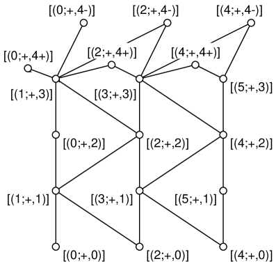
Figure 4: The graph for an exceptional NIM-rep of the diagonal coset $SU(2)_{5}\times SU(2)_{3}/SU(2)_{8}$, which originates from the conformal embedding $su(2)_{3}\oplus su(2)_{8}\subset C_{3,1}$. There are 18 Cardy states. The lines stand for the fusion with $(1,0;1)$.

For comparison, we also give the graph for the regular NIM-rep of $SU(2)_{5}\times SU(2)_{3}/SU(2)_{8}$ in Fig.5.

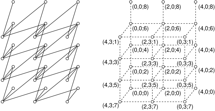
Figure 5: The regular NIM-rep of the $SU(2)_{5}\times SU(2)_{3}/SU(2)_{8}$ coset model. The left figure expresses the fusion with ${(1,0;1)}$, whereas the right one shows the labels of the corresponding Cardy states. The dashed lines are for indicating the relative position of the vertices. Here we give only the half of the Cardy states. Total number of the Cardy states are $\lvert\hat{\mathcal{I}}\rvert=54=27\times 2$. The other half is the same graph with the change that the second entry of the labels are replaced by $0\rightarrow 2$ and $3\rightarrow 1$, respectively.

One can see that this NIM-rep corresponds to the physical modular invariant $Z_{\mathcal{E}^{(3,8)}}$ of $SU(2)_{5}\times SU(2)_{3}/SU(2)_{8}$ constructed in [24],

$$\begin{split}Z_{\mathcal{E}^{(3,8)}}=\sum_{\mu=0,2,4}\,\,\Bigl{[}&\lvert\chi_{(\mu,0;0)}+\chi_{(\mu,0;8)}\rvert^{2}+\lvert\chi_{(\mu,0;4)}\rvert^{2}+\lvert\chi_{(\mu,2;2)}+\chi_{(\mu,2;6)}\rvert^{2}+\lvert\chi_{(\mu,2;4)}\rvert^{2}\\ &+(\chi_{(\mu,0;2)}+\chi_{(\mu,0;6)})\chi_{(\mu,2;4)}^{*}+\chi_{(\mu,2;4)}(\chi_{(\mu,0;2)}+\chi_{(\mu,0;6)})^{*}\\ &+\chi_{(\mu,0;4)}(\chi_{(\mu,2;0)}+\chi_{(\mu,2;8)})^{*}+(\chi_{(\mu,2;0)}+\chi_{(\mu,2;8)})\chi_{(\mu,0;4)}^{*}\Bigr{]},\end{split}$$ (4.57)

where $\chi_{(\lambda,\mu;\nu)}$ are the characters of the coset theory. The set of the primary fields which appear in the diagonal terms of $Z_{\mathcal{E}^{(3,8)}}$, i.e., the spectrum of the Ishibashi states, precisely coincides with $\hat{\mathcal{E}}$ in eq.(4.52). Hence, the NIM-rep defined in eq.(4.54) is associated with this modular invariant and is considered to be a physical one. The reason for the coincidence of the spectra is that our NIM-rep (4.54) is constructed exactly in the same way as the modular invariant $Z_{\mathcal{E}^{(3,8)}}$. This modular invariant follows from that for the tensor product theory $SU(2)_{5}\times SU(2)_{3}\times SU(2)_{8}$, which is obtained by the conformal embedding $su(2)_{3}\oplus su(2)_{8}\subset C_{3,1}$ [24]. It is therefore natural that the spectrum of $Z_{\mathcal{E}^{(3,8)}}$ is the same as $\hat{\mathcal{E}}$, which is also based on the conformal embedding into $C_{3,1}$.

5 Summary and Discussion

In this paper, we have developed a systematic procedure to construct NIM-reps in coset conformal field theories. Based on the relation of the $G/H$ theory with the $G\times H$ theory, we have shown that any NIM-rep of the $G\times H$ theory yields a NIM-rep of the $G/H$ theory. The action of the simple currents on generic NIM-reps plays an essential role in our construction. In particular, we have identified the NIM-rep version of the field identification and the selection rule, which was first observed in [18]. Combined with the conformal embedding of $G\times H$, our method provides a new class of NIM-reps which cannot be factorized into the $G$ and the $H$ parts. As an illustrative example of our procedure, the diagonal coset $SU(2)_{5}\times SU(2)_{3}/SU(2)_{8}$ has been studied in detail.

Toward the classification of the NIM-reps in coset theories, the most important question is whether our map from the $G\times H$ theory to the $G/H$ theory gives all the NIM-reps in the coset theory. In other words, we should clarify whether our map is onto or not. If this is the case, the classification problem for the coset theory reduces to that for the corresponding tensor product theory. However, the existence of the brane identification fixed points makes the problem difficult to study. To obtain a NIM-rep of the coset theory, we have to resolve brane identification fixed points, which appear even if there are no fixed points in the field identification. If there are several ways to resolve the brane identification fixed points, our map is not onto and we have to solve the problem in two steps. We note that our map is not one-to-one. More than one NIM-reps in the tensor product theory are mapped to the same NIM-rep in the coset theory, as we have encountered in several examples in this paper.

Another important problem is the issue of the physical NIM-reps. Although our method provides NIM-reps in the coset theory, it does not assures the existence of the corresponding modular invariant. It is necessary to find a criterion for our map to give a physical NIM-rep, such as that obtained in [24] for the modular invariant.

Our construction makes possible a parallel treatment of the $G$ and the $H$ sectors of the $G/H$ theory. In a sense, one can mix the boundary conditions of two sectors. It is therefore interesting to clarify the corresponding boundary condition and geometrical meaning in the sigma model approach, namely, the gauged WZW models [14, 15, 16, 17, 19, 23].

The related issue is the application of our method to the construction of $D$-branes in non-trivial backgrounds, e.g., the Kazama-Suzuki models [41]. Recently, it has been found that there exist exotic D-branes in simple backgrounds such as $c=1$ CFTs [42, 43, 44, 45] that break the isometry of the target space but keep the (super) conformal invariance on the worldsheet. It would be interesting to examine whether our construction gives the similar branes in the Kazama-Suzuki models.

Acknowledgement: The work of T.T. is supported by the Grant-in-Aid for Scientific Research on Priority Areas (2) 14046201 from the Ministry of Education, Culture, Science, Sports and Technology of Japan.

Appendix A The $E_{6}$ NIM-rep of $su(2)_{10}$ from conformal embedding

In this appendix, we illustrate the method of the conformal embedding presented in Section 2.3.2 by the example $su(2)_{10}\subset sp(4)_{1}$. The resulting NIM-rep is the $E_{6}$ NIM-rep of the $SU(2)$ WZW model [11, 8].

We begin with the branching rule of the embedding $su(2)_{10}\subset sp(4)_{1}$. The spectrum $\mathcal{I}$ of the $Sp(4)$ WZW model at level 1 is given by the set of all the integrable representations of $sp(4)=C_{2}$ at level 1, which are labeled by the horizontal part of the Dynkin label,

$$\mathcal{I}=P_{+}^{1}(sp(4))=\{(0,0),\,(1,0),\,(0,1)\}.$$ (A.1)

Similarly, the spectrum $\tilde{\mathcal{I}}$ of the $SU(2)$ WZW model at level 10 reads

$$\tilde{\mathcal{I}}=P_{+}^{10}(su(2))=\{(\tilde{\mu})\,|\,\tilde{\mu}=0,1,\ldots,10\}.$$ (A.2)

The branching rule (2.44) can be written as follows,

$$h=0 :(0,0)\mapsto(0)\operatorname*{\oplus}(6),$$

$$h=5/16 :(1,0)\mapsto(3)\operatorname*{\oplus}(7),$$ (A.3)

$$h=1/2 :(0,1)\mapsto(4)\operatorname*{\oplus}(10).$$

Here $h$ is the conformal dimension of each representation in $\mathcal{I}$. The dimension $\tilde{h}_{\tilde{\mu}}$ of $\tilde{\mu}\in\tilde{\mathcal{I}}$ is given by

$$\tilde{h}_{\tilde{\mu}}=\frac{1}{48}\tilde{\mu}(\tilde{\mu}+2),$$ (A.4)

and consistent with the branching rule (A). The modular $S$-matrix of $sp(4)_{1}$ takes the form

$$S=\frac{1}{2}\begin{pmatrix}1&\sqrt{2}&1\\ \sqrt{2}&0&-\sqrt{2}\\ 1&-\sqrt{2}&1\end{pmatrix},$$ (A.5)

where the rows and columns are ordered as in (A.1). For $su(2)_{10}$, the formula (3.17) yields

$$\tilde{S}_{\tilde{\mu}\tilde{\nu}}=\frac{1}{\sqrt{6}}\sin\Bigl{(}\frac{\pi}{12}(\tilde{\mu}+1)(\tilde{\nu}+1)\Bigr{)}.$$ (A.6)

One can confirm that the branching rule (A) is compatible with the modular transformations $S$ and $\tilde{S}$.

The starting point of our construction is the regular NIM-rep $\psi_{\alpha}{}^{\mu}=S_{\alpha\mu}$ of $sp(4)_{1}$. Hence, at the beginning, we have three Ishibashi states and three Cardy states labelled by $\mathcal{E}=\mathcal{V}=\mathcal{I}$. According to the formula (2.45) and the branching rule (A), the Ishibashi states of $sp(4)_{1}$ can be decomposed into those of $su(2)_{10}$ as follows,

$$\begin{split}|(0,0)\rangle\!\rangle&=a|0\rangle\!\rangle+b|6\rangle\!\rangle,\\ |(1,0)\rangle\!\rangle&=\frac{1}{\sqrt{2}}(|3\rangle\!\rangle+|7\rangle\!\rangle),\\ |(0,1)\rangle\!\rangle&=b|4\rangle\!\rangle+a|10\rangle\!\rangle,\end{split}$$ (A.7)

where

$$a=\sqrt{\frac{2\sin(\pi/12)}{\sqrt{6}}}=\sqrt{\frac{3-\sqrt{3}}{6}},\quad\quad b=\sqrt{\frac{2\sin(5\pi/12)}{\sqrt{6}}}=\sqrt{\frac{3+\sqrt{3}}{6}}.$$ (A.8)

From this expression, one can read off the set $\tilde{\mathcal{E}}$ of the labels of the $su(2)$ Ishibashi states,

$$\tilde{\mathcal{E}}=\{0,\,3,\,4,\,6,\,7,\,10\}.$$ (A.9)

Using eq.(A.7), the Cardy states of $sp(4)_{1}$ can be regarded as the boundary states of $su(2)_{10}$. Since $\lvert\tilde{\mathcal{E}}\rvert=6$, the Cardy state $|\alpha\rangle$ is expressed as a six-dimensional (row) vector $\tilde{\psi}_{\alpha}$ (see eq.(2.48)),

$$\begin{pmatrix}\tilde{\psi}_{(0,0)}\\ \tilde{\psi}_{(0,1)}\\ \tilde{\psi}_{(1,0)}\end{pmatrix}=\begin{pmatrix}a/2&1/2&b/2&b/2&1/2&a/2\\ a/2&-1/2&b/2&b/2&-1/2&a/2\\ a/\sqrt{2}&0&-b/\sqrt{2}&b/\sqrt{2}&0&-a/\sqrt{2}\end{pmatrix},$$ (A.10)

where the columns are ordered as in (A.9).

Let us apply the boundary state generating technique in Section 2.3.2 to the above states. Since $\lvert\tilde{\mathcal{E}}\rvert-\lvert\mathcal{V}\rvert=3$, there are three states missing. We consider the fusion of $\tilde{\psi}_{(0,0)}$ with the generator $(1)\in\tilde{\mathcal{I}}$ of the fusion algebra. The fusion of $\tilde{\psi}_{(0,0)}$ with $(1)$ yields the vector $\tilde{\psi}_{(0,0)}\gamma^{(1)}$, where the generalized quantum dimension $\gamma^{(1)}$ reads

$$\gamma^{(1)}=\mathrm{diag}\biggl{(}\frac{\tilde{S}_{1\tilde{\mu}}}{\tilde{S}_{0\tilde{\mu}}}\biggr{)}_{\tilde{\mu}\in\tilde{\mathcal{E}}}=\mathrm{diag}\bigl{(}\sqrt{6}b^{2},1,\sqrt{6}a^{2},-\sqrt{6}a^{2},-1,\sqrt{6}b^{2}\bigr{)}.$$ (A.11)

One can easily show that the length of the vector $\tilde{\psi}_{(0,0)}\gamma^{(1)}$ is 1, which means that this vector gives one of the Cardy states. None of the three vectors in $\mathcal{V}$ coincides with this vector. Hence $\tilde{\psi}_{(0,0)}\gamma^{(1)}$ gives a new state

$$\tilde{\psi}_{2}=\tilde{\psi}_{(0,0)}\gamma^{(1)}.$$ (A.12)

Repeating this process for $\tilde{\psi}_{2}$, we obtain $\lVert\tilde{\psi}_{2}\gamma^{(1)}\rVert^{2}=2$, which means that $\tilde{\psi}_{2}\gamma^{(1)}$ contains two Cardy states. One can easily identify one of the Cardy states with $\tilde{\psi}_{(0,0)}$, since $(\tilde{\psi}_{2}\gamma^{(1)},\tilde{\psi}_{(0,0)})=\tilde{\psi}_{2}\gamma^{(1)}\tilde{\psi}_{(0,0)}{}^{\dagger}=1$. Subtracting $\tilde{\psi}_{(0,0)}$ from $\tilde{\psi}_{2}\gamma^{(1)}$, we obtain a new vector

$$\tilde{\psi}_{3}=\tilde{\psi}_{2}\gamma^{(1)}-\tilde{\psi}_{(0,0)}.$$ (A.13)

The fusion of $\tilde{\psi}_{3}$ also yields a new state

$$\tilde{\psi}_{4}=\tilde{\psi}_{3}\gamma^{(1)}-\tilde{\psi}_{2}-\tilde{\psi}_{(1,0)}.$$ (A.14)

The fusion of $\tilde{\psi}_{4}$ however gives no new states

$$\tilde{\psi}_{4}\gamma^{(1)}=\tilde{\psi}_{(0,1)}+\tilde{\psi}_{3},$$ (A.15)

and the generating process terminates here. We have therefore obtained six mutually independent Cardy states, which are labelled by the set

$$\tilde{\mathcal{V}}=\{1=(0,0),\,2,\,3,\,4,\,5=(0,1),\,6=(1,0)\}.$$ (A.16)

The explicit form of the matrix $\tilde{\psi}$ reads

$$\tilde{\psi}=\begin{pmatrix}\tilde{\psi}_{1}=\tilde{\psi}_{(0,0)}\\ \tilde{\psi}_{2}\\ \tilde{\psi}_{3}\\ \tilde{\psi}_{4}\\ \tilde{\psi}_{5}=\tilde{\psi}_{(0,1)}\\ \tilde{\psi}_{6}=\tilde{\psi}_{(1,0)}\end{pmatrix}=\begin{pmatrix}a/2&1/2&b/2&b/2&1/2&a/2\\ b/2&1/2&a/2&-a/2&-1/2&-b/2\\ b/\sqrt{2}&0&-a/\sqrt{2}&-a/\sqrt{2}&0&b/\sqrt{2}\\ b/2&-1/2&a/2&-a/2&1/2&-b/2\\ a/2&-1/2&b/2&b/2&-1/2&a/2\\ a/\sqrt{2}&0&-b/\sqrt{2}&b/\sqrt{2}&0&-a/\sqrt{2}\end{pmatrix},$$ (A.17)

which coincides with the diagonalization matrix of the $E_{6}$ NIM-rep of $su(2)_{10}$ [11, 8].

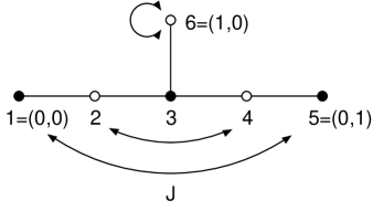
Figure 6: The $E_{6}$ NIM-rep from the conformal embedding $su(2)_{10}\subset sp(4)_{1}$. Each vertex corresponds to the Cardy state. The solid line stands for the fusion with $(1)$. The arrows show the action of the simple current $J=(10)$ on the Cardy states. A black (white) vertex has $\tilde{b}=1$ ($\tilde{b}=-1$). (see eq.(2.36b))

We show the result in Fig.6 together with the action of the simple current (2.36).

Appendix B Construction of NIM-reps in the $SU(3)_{1}\times SU(3)_{1}$ $/SU(3)_{2}$ model

In this appendix, we apply the method developed in Section 4.2 to the diagonal coset $SU(3)_{1}\times SU(3)_{1}/SU(3)_{2}$. We start from the simple current NIM-reps of the $SU(3)_{1}\times SU(3)_{1}\times SU(3)_{2}$ model with the sets $\mathcal{E}$ and $\mathcal{V}$. Since the representations of $su(3)$ are in general not real, we have to distinguish $\mathcal{E}^{c}$ with $\mathcal{E}$ (see eq.(4.22)). Hence, this model is a simple example for illustrating the meaning of the charge conjugation $\mathcal{E}\rightarrow\mathcal{E}^{c}$, which plays an essential role in the construction of NIM-reps in the coset theories.

The set of the primary fields of the $SU(3)_{1}\times SU(3)_{1}\times SU(3)_{2}$ theory is given by

$$\mathcal{I}=\{(\lambda,\mu,\nu)\,|\,\lambda,\mu\in P_{+}^{1}(su(3));\,\nu\in P_{+}^{2}(su(3))\},$$ (B.1)

where

$$P_{+}^{1}(su(3))=\{00,\,10,\,01\},\quad P_{+}^{2}(su(3))=\{00,\,20,\,02,\,11,\,01,\,10\},$$ (B.2)

and $(\lambda_{1}\lambda_{2})$ are the Dynkin labels of $su(3)$. The simple current group of $su(3)_{k}$ are generated by $(k0)$ and isomorphic to $\mathbb{Z}_{3}$,

$$G_{\mathrm{sc}}(su(3)_{k})=\{1=(00),J=(k0),J^{2}=(0k)\}\cong\mathbb{Z}_{3},$$ (B.3)

which acts on $P_{+}^{1}(su(3))$ and $P_{+}^{2}(su(3))$ as

$$\begin{split}J:&~{}00\rightarrow 10\rightarrow 01\rightarrow 00,\\ J:&~{}00\rightarrow 20\rightarrow 02\rightarrow 00~{},~{}11\rightarrow 01\rightarrow 10\rightarrow 11.\end{split}$$ (B.4)

The monodromy charge is given by

$$b_{\lambda}(J)=\exp\biggl{(}\frac{2\pi i}{3}(\lambda_{1}+2\lambda_{2})\biggr{)}.$$ (B.5)

The simple current group $G_{\mathrm{sc}}$ of $SU(3)_{1}\times SU(3)_{1}\times SU(3)_{2}$ is the direct product of each factor,

$$G_{\mathrm{sc}}=\{(J^{l},J^{m},J^{n})|\,l,m,n=0,1,2\}\cong\mathbb{Z}_{3}\times\mathbb{Z}_{3}\times\mathbb{Z}_{3}.$$ (B.6)

As is discussed in Section 2.3.1, we can construct the simple current NIM-rep of the product theory for any subgroup $H$ of $G_{\mathrm{sc}}$. Here we take the following $H$,

$$H=\{(1,1,1),\,(1,J,J),\,(1,J^{2},J^{2})\}\cong\mathbb{Z}_{3}.$$ (B.7)

Since the action of $H$ has no fixed points, we can use the formula (2.39) to obtain the simple current NIM-rep,

$$\psi_{(\alpha:\beta:\gamma)}{}^{(\lambda,\mu,\nu)}=\sqrt{3}S^{(1)}_{\alpha\lambda}S^{(1)}_{\beta\mu}S^{(2)}_{\gamma\nu},\quad(\alpha:\beta:\gamma)\in\mathcal{V},\,\,(\lambda,\mu,\nu)\in\mathcal{E},$$ (B.8)

where $S^{(k)}$ is the modular transformation $S$-matrix of $su(3)_{k}$. The sets $\mathcal{V}$ and $\mathcal{E}$ are defined as follows,

$$\begin{split}\mathcal{V}&=\{(\alpha:\beta:\gamma)|\,(\alpha,\beta,\gamma)\in\mathcal{I},(\alpha:J\beta:J\gamma)=(\alpha:\beta:\gamma)\}\\ &=\{(\alpha:\beta:00),(\alpha:\beta:11)|\,\alpha,\beta\in P_{+}^{1}(su(3))\},\\ \mathcal{E}&=\{(\lambda,\mu,\nu)\in\mathcal{I}\,|\,b_{\mu}(J)b_{\nu}(J)=1\}\\ &=\{(\lambda,00,00),(\lambda,00,11),(\lambda,10,20),(\lambda,10,01),\\ &\quad\quad(\lambda,01,02),(\lambda,01,10)|\,\lambda\in P_{+}^{1}(su(3))\}.\end{split}$$ (B.9)

Next, we use the procedure in Section 4.2 to obtain the corresponding NIM-rep in the $SU(3)_{1}\times SU(3)_{1}$ $/SU(3)_{2}$ theory. Applying the charge conjugation $\overline{(\lambda_{1}\lambda_{2})}=(\lambda_{2}\lambda_{1})$ to $\mathcal{E}$, we obtain the set $\mathcal{E}^{c}$,

$$\begin{split}\mathcal{E}^{c}&=\{(\lambda,00,00),(\lambda,00,11),(\lambda,10,02),(\lambda,10,10),\\ &\quad\quad(\lambda,01,20),(\lambda,01,01)|\,\lambda\in P_{+}^{1}(su(3))\}.\end{split}$$ (B.10)

Note that $\mathcal{E}^{c}\neq\mathcal{E}$. Since the stabilizer of $\mathcal{V}^{c}$ is $H$, the automorphism groups for $\mathcal{E}^{c}$ and $\mathcal{V}^{c}$ read

$$\begin{split}G(\mathcal{E}^{c})&=\{(J^{n},1,1),(J^{n},J,J^{2}),(J^{n},J^{2},J)|\,n=0,1,2\}\cong\mathbb{Z}_{3}\times\mathbb{Z}_{3},\\ G(\mathcal{V}^{c})&=G_{\mathrm{sc}}/H\cong\mathbb{Z}_{3}\times\mathbb{Z}_{3}.\end{split}$$ (B.11)

The identification current group is

$$G_{\mathrm{id}}=\{(J^{n},J^{n},J^{n})\,|\,n=0,1,2\}\cong\mathbb{Z}_{3},$$ (B.12)

whereas the identification groups for $\mathcal{E}^{c}$ and $\mathcal{V}^{c}$ are

$$\begin{split}G_{\mathrm{id}}(\mathcal{E}^{c})&=G_{\mathrm{id}}\cap G(\mathcal{E}^{c})=\{(1,1,1)\},\\ G_{\mathrm{id}}(\mathcal{V}^{c})&=G_{\mathrm{id}}/(G_{\mathrm{id}}\cap H)=G_{\mathrm{id}}.\end{split}$$ (B.13)

The brane identification group $G_{\mathrm{id}}(\mathcal{V}^{c})\cong\mathbb{Z}_{3}$ acts on $\mathcal{V}^{c}$ as

$$J:\,(\alpha:\beta:\gamma)\rightarrow(J\alpha:J\beta:J\gamma)=(J\alpha:\beta:\gamma).$$ (B.14)

From eqs.(4.32) (4.34), we obtain

$$\begin{split}\hat{\mathcal{E}}&=\{(00,00;00),(00,00;11),(00,10;10),(00,10;02),(00,01;01),(00,01;20)\},\\ \hat{\mathcal{V}}&=\{[(00:00:00)],[(00:00:11)],[(00:10:00)],\\ &\quad\quad[(00:10:11)],[(00:01:00)],[(00:01:11)]\}.\end{split}$$ (B.15)

The diagonalization matrix follows from the formula (4.36a),

$$\hat{\psi}_{[(\alpha:\beta:\gamma)]}{}^{(\lambda,\mu;\nu)}=\sqrt{\lvert G_{\mathrm{id}}(\mathcal{E}^{c})\rvert\lvert G_{\mathrm{id}}(\mathcal{V}^{c})\rvert}\psi_{(\alpha:\beta:\gamma)}{}^{(\lambda,\mu,\bar{\nu})}=3S^{(1)}_{\alpha\lambda}S^{(1)}_{\beta\mu}S^{(2)}_{\gamma\bar{\nu}}=\hat{S}_{(\alpha,\beta;\gamma)(\lambda,\mu;\nu)},$$ (B.16)

where $\hat{S}$ is the $S$-matrix of the coset theory. The resulting NIM-rep is nothing but the regular NIM-rep of the coset theory and manifestly physical. In this coset theory, there is another NIM-rep which follows from the twisted boundary condition of $su(3)$ [18]. The twisted NIM-rep is also constructed as the simple current NIM-rep by taking an appropriate $H$, e.g., a subgroup generated by $(1,J,J^{2})$.

References

- [1] J. L. Cardy, “Boundary conditions, fusion rules and the Verlinde formula”, Nucl. Phys. B 324 (1989) 581.
- [2] J. L. Cardy and D. C. Lewellen, “Bulk and boundary operators in conformal field theory,” Phys. Lett. B 259 (1991) 274.
- [3] D. C. Lewellen, “Sewing constraints for conformal field theories on surfaces with boundaries,” Nucl. Phys. B 372 (1992) 654.
- [4] G. Pradisi, A. Sagnotti and Y. S. Stanev, “Completeness Conditions for Boundary Operators in 2D Conformal Field Theory,” Phys. Lett. B 381 (1996) 97 [hep-th/9603097].
- [5] I. Runkel, “Boundary structure constants for the A-series Virasoro minimal models,” Nucl. Phys. B 549 (1999) 563 [hep-th/9811178]; “Structure constants for the D-series Virasoro minimal models,” Nucl. Phys. B 579 (2000) 561 [hep-th/9908046].
- [6] J. Fuchs and C. Schweigert, “Symmetry breaking boundaries. I: General theory,” Nucl. Phys. B 558 (1999) 419 [hep-th/9902132]; “Symmetry breaking boundaries. II: More structures, examples,” Nucl. Phys. B 568 (2000) 543 [hep-th/9908025].
- [7] L. Birke, J. Fuchs and C. Schweigert, “Symmetry breaking boundary conditions and WZW orbifolds,” Adv. Theor. Math. Phys. 3 (1999) 671 [hep-th/9905038].
- [8] R. E. Behrend, P. A. Pearce, V. B. Petkova and J. B. Zuber, “Boundary conditions in rational conformal field theories,” Nucl. Phys. B 570 (2000) 525 [Nucl. Phys. B 579 (2000) 707] [hep-th/9908036].
- [9] G. Felder, J. Fröhlich, J. Fuchs and C. Schweigert, “Conformal boundary conditions and three-dimensional topological field theory,” Phys. Rev. Lett. 84 (2000) 1659 [hep-th/9909140]; “Correlation functions and boundary conditions in RCFT and three-dimensional topology,” hep-th/9912239.
- [10] I. Brunner and V. Schomerus, “On superpotentials for D-branes in Gepner models,” JHEP 0010 (2000) 016 [hep-th/0008194].
- [11] P. Di Francesco and J. B. Zuber, “SU(N) Lattice integrable models associated with graphs,” Nucl. Phys. B 338 (1990) 602.
- [12] T. Gannon, “Boundary conformal field theory and fusion ring representations,” Nucl. Phys. B 627 (2002) 506 [hep-th/0106105].
- [13] P. Goddard, A. Kent and D. I. Olive, “Virasoro algebras and coset space models,” Phys. Lett. B 152 (1985) 88; “Unitary representations of the Virasoro and supervirasoro algebras,” Commun. Math. Phys. 103 (1986) 105.
- [14] J. Maldacena, G. W. Moore and N. Seiberg, “Geometrical interpretation of D-branes in gauged WZW models,” JHEP 0107 (2001) 046 [hep-th/0105038].
- [15] K. Gawȩdzki, “Boundary WZW, G/H, G/G and CS theories,” hep-th/0108044.
- [16] S. Elitzur and G. Sarkissian, “D-branes on a gauged WZW model,” Nucl. Phys. B 625 (2002) 166 [hep-th/0108142].
- [17] S. Fredenhagen and V. Schomerus, “D-branes in coset models,” JHEP 0202 (2002) 005 [hep-th/0111189].
- [18] H. Ishikawa, “Boundary states in coset conformal field theories,” Nucl. Phys. B 629 (2002) 209 [hep-th/0111230].
- [19] T. Kubota, J. Rasmussen, M. A. Walton and J. G. Zhou, “Maximally symmetric D-branes in gauged WZW models,” Phys. Lett. B 544 (2002) 192 [hep-th/0112078].
- [20] M. Nozaki, “Comments on D-branes in Kazama-Suzuki models and Landau-Ginzburg theories,” JHEP 0203 (2002) 027 [hep-th/0112221].
- [21] T. Quella and V. Schomerus, “Symmetry breaking boundary states and defect lines,” JHEP 0206 (2002) 028 [hep-th/0203161].
- [22] S. Fredenhagen and V. Schomerus, “On boundary RG-flows in coset conformal field theories,” hep-th/0205011.
- [23] M. A. Walton and J. G. Zhou, “D-branes in asymmetrically gauged WZW models and axial-vector duality,” hep-th/0205161.
- [24] T. Gannon and M. A. Walton, “On the classification of diagonal coset modular invariants,” Commun. Math. Phys. 173 (1995) 175 [hep-th/9407055].
- [25] A. N. Schellekens and S. Yankielowicz, “Extended chiral algebras and modular invariant partition functions,” Nucl. Phys. B 327 (1989) 673; “Simple currents, modular invariants and fixed points,” Int. J. Mod. Phys. A 5 (1990) 2903.
- [26] K. A. Intriligator, “Bonus symmetry in conformal field theory,” Nucl. Phys. B 332 (1990) 541.
-
[27]
M. R. Gaberdiel and T. Gannon,
“Boundary states for WZW models,”
Nucl. Phys. B 639 (2002) 471 [hep-th/0202067]. - [28] N. Ishibashi, “The boundary and crosscap states in conformal field theories”, Mod. Phys. Lett. A4 (1989) 251.
- [29] E. Verlinde, “Fusion rules and modular transformations in 2-D conformal field theory,” Nucl. Phys. B 300 (1988) 360.
- [30] J. Fuchs, L. R. Huiszoon, A. N. Schellekens, C. Schwiegert and J. Walcher, “Boundaries, crosscaps and simple currents,” Phys. Lett. B 495 (2000) 427 [hep-th/0007174].
- [31] F. Xu, “New braided endomorphisms from conformal inclusions, ” Commun. Math. Phys. 192 (1998) 349.
- [32] J. Böckenhauer and D. E. Evans, “Modular invariants, graphs and -induction for nets of subfactors. I, II, III” Commun. Math. Phys. 197 (1998) 361 [hep-th/9801171]; ibid. 200 (1999) 57 [hep-th/9805023]; ibid. 205 (1999) 183 [hep-th/9812110].
- [33] J. Böckenhauer, D. E. Evans and Y. Kawahigashi, “Chiral structure of modular invariants for subfactors,” Commun. Math. Phys. 210 (2000) 733 [math.OA/9907149]; “Longo-Rehren subfactors arising from -induction,” math.OA/0002154
- [34] J. Fuchs and C. Schweigert, “Solitonic sectors, -induction and symmetry breaking boundaries,” Phys. Lett. B 490 (2000) 163 [hep-th/0006181].
- [35] A. N. Schellekens and N. P. Warner, “Conformal subalgebras of Kac-Moody algebras,” Phys. Rev. D 34 (1986) 3092.
- [36] F. A. Bais and P. G. Bouwknegt, “A classification of subgroup truncations of the bosonic string,” Nucl. Phys. B 279 (1987) 561.
- [37] D. Bernard, “String characters from Kac-Moody automorphisms,” Nucl. Phys. B 288 (1987) 628.
- [38] Y. S. Stanev, “Classification of the local extension of the SU(2) SU(2) chiral current algebras, ” J. Math. Phys. 36 (1995) 2070.
- [39] J. Fuchs, B. Schellekens and C. Schweigert, “The resolution of field identification fixed points in diagonal coset theories,” Nucl. Phys. B 461 (1996) 371 [hep-th/9509105].
- [40] D. C. Dunbar and K. G. Joshi, “Characters for coset conformal field theories,” Int. J. Mod. Phys. A 8 (1993) 4103 [hep-th/9210122]; “Maverick examples of coset conformal field theories,” Mod. Phys. Lett. A 8 (1993) 2803 [hep-th/9309093].
- [41] Y. Kazama and H. Suzuki, “New superconformal field theories and superstring compactification,” Nucl. Phys. B 321 (1989) 232.
- [42] M. R. Gaberdiel, A. Recknagel and G. M. Watts, “The conformal boundary states for SU(2) at level 1,” Nucl. Phys. B 626 (2002) 344 [hep-th/0108102].
- [43] M. R. Gaberdiel and A. Recknagel, “Conformal boundary states for free bosons and fermions,” JHEP 0111 (2001) 016 [hep-th/0108238].
- [44] R. A. Janik, “Exceptional boundary states at ,” Nucl. Phys. B 618 (2001) 675 [hep-th/0109021].
- [45] L. S. Tseng, “A note on c = 1 Virasoro boundary states and asymmetric shift orbifolds,” JHEP 0204 (2002) 051 [hep-th/0201254].