LBNL-51261
UCB-PTH-02/32
hep-th/0207174
On Continuous Moyal Product Structure in String Field Theory

Abstract

We consider a diagonalization of Witten’s star product for a ghost system of arbitrary background charge and Grassmann parity. To this end we use a bosonized formulation of such systems and a spectral analysis of Neumann matrices. We further identify a continuous Moyal product structure for a combined ghosts+matter system. The normalization of multiplication kernel is discussed.

1 Introduction

A representation of Witten’s star product in open string field theory (SFT) [1] as a family of infinitely many Moyal products was first proposed by I. Bars in [2]. The approach of that paper is essentially based on split formalism in SFT, it was further elaborated in papers [2], [3]. A different approach to Moyal-type representation for Witten’s star product based on spectroscopy of Neumann matrices [4] was taken up in [5]. The authors of that paper showed that in the matter sector the Witten’s star can be represented as a continuous Moyal product specified by a family of noncommutativity parameters

$$\theta(\kappa)=2\tanh\left(\frac{\pi\kappa}{4}\right)$$

labelled by a continuous variable $0\leq\kappa<\infty$. An additional assumption in that paper was the restriction to zero momentum sector. The whole construction was generalized to arbitrary momentum in [6].

One hopes that reformulation of string field theory that uses a continuous Moyal product will make the whole structure more transparent and introduce new computational tools. Given the fact that SFT axioms [1] mimic the conventional axioms of noncommutative geometry [7], the theory written in some new basis may ultimately resemble a lot noncommutative field theories (see [8], [9], [10], [11], [12] for a review). Thus in noncommutative field theories solitonic solutions were explicitly constructed [13] using Moyal algebra projectors. It turns out the well known sliver solution [14] in SFT being rewritten in the continuous Moyal basis is represented by a functional

$$\Xi[x_{\alpha}(\kappa)]={\cal N}\exp\left[-\int_{0}^{\infty}d\kappa\,\frac{x_{\alpha}(\kappa)x_{\alpha}(\kappa)}{\theta(\kappa)}\right]$$

that has the form of a continuous family of noncommutative field theory projectors (see [15] for a detailed discussion of this representation of the sliver).

To complete the program and rewrite the whole SFT (VSFT or Witten’s cubic SFT) in the continuous Moyal basis one needs to extend the formalism to include the ghost sector and a BRST operator. In the present paper we extend the approach of [5] to ghosts. A preliminary work in that direction was done in [6] where ghosts in the bosonic SFT were treated in the fermionic $b$-$c$-representation. In [16] a continuous Moyal product was constructed for string fields including ghosts (in $bc$ formalism) restricted to Siegel’s gauge. In this paper we work in the bosonized representation considering ghost systems of arbitrary background charge and Grassmann parity. We find working in bosonized representation technically simpler than treating $bc$- or $\beta\gamma$-systems directly. The continuous Moyal product for fermionic fields was considered in [17].

The paper is organized as follows. In section 2 we set up some notations and remind the reader the form of two and three-string vertices for ghosts in the bosonized representation. In section 3 we diagonalize these vertices using the spectroscopy of Neumannn matrices. In section 4 we represent the Witten’s star product as a functional integral operator specified by a certain kernel. In section 5 we discuss regularization of determinants in the continuous Moyal basis. As an instructive exercise we check the cancellation of infinities for overlaps of surface states. In section 6 we apply the technique of section 5 to the normalization constant of the multiplication kernel. This section also contains further discussion of the precise correspondence between the Witten star product and the continuous Moyal one. We end with conclusions in section 7. Appendices contains technical details of the calculations.

2 Ghost $2$- and $3$-string vertices in the bosonized formulation

2.1 Bosonized formulation

In bosonized formulation a ghost $bc$- or $\beta\gamma$- system is represented by a single bosonic field $\phi(z,\bar{z})$ with a mode expansion [18, 19]

$$\epsilon\phi(z,\overline{z})=2i\phi_{0}+j_{0}\log z\overline{z}-\sum_{n\neq 0}\frac{j_{n}}{n}\left(\frac{1}{z^{n}}+\frac{1}{\overline{z}^{n}}\right)$$ (2.1a)

where $$j_{0} q\in{\mathbb{Z}} \epsilon +1 b c -1 \beta \gamma \epsilon$$ is the ghost number operator taking integral values , parameter takes values for a fermionic - system and for a bosonic - ghost system. The parameter also enters the commutation relations

$$[\phi_{0},j_{0}]=i\epsilon\quad\text{and}\quad[j_{n},j_{m}]=\epsilon n\delta_{n+m,0}\,.$$ (2.1b)

A conformal stress-energy tensor for a field $$\phi Q$$ with a background charge is given by the expression

$$T_{\phi}=\frac{\epsilon}{2}\partial\phi\partial\phi-\frac{Q}{2}\partial^{2}\phi.$$ (2.1c)

The last term in the stress energy tensor is due to the anomaly in the conservation of the ghost current $j=\epsilon\partial\phi$. The number $Q$ is a background charge, which is equal to $-3$ for conformal $bc$ ghost system of the bosonic string.

Denote by $|q\rangle$ a state that is annihilated by $j_{n}$, $n>0$ and is of ghost number $q$:

$$j_{n}|q\rangle=0\quad\text{and}\quad j_{0}|q\rangle=q|q\rangle.$$ (2.2)

Because of the anomaly in the conservation of the ghost charge the inner product is nonzero only for the following states

$$\langle-q-Q|q^{\prime}\rangle=\delta_{qq^{\prime}}.$$ (2.3)

We further introduce creation and annihilation operators according to

$$a_{n}^{\dagger}=\sqrt{n}j_{-n}\quad\text{and}\quad a_{n}=\sqrt{n}j_{n}\,,\enspace n>0\,.$$ (2.4a)

Notice that the commutation relations for these oscillators include $$\epsilon$$

$$[a_{n},\,a^{{\dagger}}_{m}]=\epsilon\delta_{nm}.$$ (2.4b)

2.2 Overlap vertices

The two operations: multiplication and inner product, needed to define string field theory action, can be written in terms of $3$- and $2$-string vertices. Here we will present only the vertices for the bosonized ghosts. The ones for the matter part can be found, for example in [20, 21, 22].

The 3-string vertex for a bosonized field (2.1c) can be written as [23, 24]

$$|V_{3}^{(\phi)}\rangle_{123}=\sum_{q_{r}\in\mathbb{Z}}\delta_{q_{1}+q_{2}+q_{3}+Q,0}\exp\left[-\frac{\epsilon}{4}V_{00}^{\prime}\Bigl{(}\sum_{r}q_{r}^{2}-Q^{2}\Bigr{)}\right.+\frac{\epsilon}{\sqrt{2}}\sum_{r,s}\sum_{n=1}^{\infty}q_{r}V_{0n}^{\prime rs}a_{n}^{(s){\dagger}}\\ -\frac{\epsilon}{2}\sum_{r,s}\sum_{n,m=1}^{\infty}a_{n}^{(r){\dagger}}V_{nm}^{\prime rs}a_{m}^{(s){\dagger}}\left.-\epsilon\frac{Q\sqrt{2}}{6}\sum_{r=1}^{3}\sum_{n=1}^{\infty}J_{n}a_{n}^{(r){\dagger}}\right]\bigotimes_{r=1}^{3}|-q_{r}-Q\rangle,$$ (2.5a)

where

$$V_{nm}^{\prime rs} =\frac{1}{3}\bigl{(}C^{\prime}+\alpha^{s-r}U^{\prime}+\alpha^{r-s}\bar{U}^{\prime}\bigr{)}_{nm}$$ (2.5b)

$$V_{0m}^{\prime rs} =\frac{1}{3}\bigl{(}\alpha^{s-r}W^{\prime}_{m}+\alpha^{r-s}\bar{W}^{\prime}_{m}\bigr{)}$$ (2.5c)

$$V_{00}^{\prime} =-2\log\gamma,\qquad\gamma=\frac{4}{3\sqrt{3}}$$ (2.5d)

are the standard $$3 C_{mn}^{\prime} (-1)^{n}\delta_{nm} J_{n}$$-string vertex matrices [20, 22], is a twist matrix and vector is given by

$$J_{2n}=\frac{(-1)^{n}}{\sqrt{n}}\quad\text{and}\quad J_{2n+1}=0\,.$$ (2.5e)

The indices $r$ and $s$ in (2.5a) run from $1$ to $3$ and label the tensorial components in the 3-string Hilbert space. Essentially (2.5a) differs from the matter vertex by the presence of the background charge in the Kronecker symbol and the term linear in $Q$ in the exponent which arises from the insertion of the operator [20]

$$\exp\left[-\frac{\epsilon Q}{12}\sum_{r=1}^{3}\phi^{(r)}\Bigl{(}\frac{\pi}{2}\Bigr{)}\right]$$ (2.6)

into the vertex (2.5a) with $Q=0$.

As a side remark we would like to note that the exponent here is not normal ordered. Formally, if one acts by the operator (2.6) on the vertex (2.5a) with $Q=0$, one obtains an extra numeric factor

$$\exp\left[-\frac{\epsilon Q^{2}}{24}\sum_{n=1}^{\infty}J_{n}^{2}\right]\,.$$

This factor is important for the overall normalization of the vertex, our normalization coincides with the one in [23]. Notice also that the quadratic term in the vertex exponential is exactly the same as that of the matter part upon the substitution $\epsilon\mapsto g_{\mu\nu}$.

The 2-string vertex reads [23]

$$|V_{2}^{(\phi)}\rangle_{12}=\sum_{q\in{\mathbb{Z}}}\exp\left[-\epsilon\sum_{n=1}^{\infty}a_{n}^{(1)\dagger}(-1)^{n}a_{n}^{(2)\dagger}\right]|q\rangle_{1}\otimes|-q-Q\rangle_{2}\,.$$ (2.7)

It realizes the $\mathop{\mathrm{bpz}}\nolimits$ conjugation on the modes of field $\phi$.

3 Diagonalization

3.1 Notations

The diagonalization of the matter vertex (at zero momentum) found in [5] is based on the spectral analysis of Neumann matrices done in [4]. It was shown in [4] that the matrices $(C^{\prime}V^{\prime})_{mn}^{rs}$ have a joint set of eigenvectors $v_{n}^{(\kappa)}$ labeled by a continuous parameter $-\infty<\kappa<\infty$. Namely we have

$$\sum_{n}(C^{\prime}V^{\prime rs})_{mn}v_{n}^{(\kappa)}=\mu^{rs}(\kappa)v_{m}^{(\kappa)}$$

where

$$\mu^{rs}(\kappa)=\frac{1}{1+2\cosh\frac{\pi\kappa}{2}}\Bigl{[}1-2\delta_{r,s}+e^{\frac{\pi\kappa}{2}}\delta_{r+1,s}+e^{-\frac{\pi\kappa}{2}}\delta_{r,s+1}\Bigr{]}.$$ (3.1)

The vectors $v^{(\kappa)}$ are chosen to satisfy the following orthogonality and completeness relations [25]

$$(v^{(\kappa)},v^{(\kappa^{\prime})})=\mathcal{N}(\kappa)\delta(\kappa-\kappa^{\prime})\quad\text{and}\quad\int_{-\infty}^{+\infty}\frac{d\kappa}{\mathcal{N}(\kappa)}\,v_{m}^{(\kappa)}v_{n}^{(\kappa)}=\delta_{mn}$$ (3.2)

where

$$\mathcal{N}(\kappa)=\frac{2}{\kappa}\sinh\left(\frac{\pi\kappa}{2}\right)\,.$$ (3.3)

We use $v^{(\kappa)}$ to introduce a new oscillator basis

$$a_{\kappa}^{{\dagger}}=\frac{1}{\sqrt{\mathcal{N}(\kappa)}}\sum_{n=1}^{\infty}a_{n}^{{\dagger}}v^{(\kappa)}_{n}\,$$ (3.4)

and the same for $a_{\kappa}$. The action of the operator $C^{\prime}$ and commutation relations are of the form

$$C^{\prime}a_{\kappa}^{{\dagger}}=-a_{-\kappa}^{{\dagger}}\quad\text{and}\quad[a_{\kappa},\,a_{\kappa^{\prime}}^{{\dagger}}]=\epsilon\delta(\kappa-\kappa^{\prime}).$$ (3.5)

We next perform one more change of the oscillator basis which diagonalizes the operator $C^{\prime}$

$$e_{\kappa}^{{\dagger}} =\frac{a_{\kappa}^{{\dagger}}+C^{\prime}a_{\kappa}^{{\dagger}}}{\sqrt{2}}, \qquad o_{\kappa}^{{\dagger}} =\frac{a_{\kappa}^{{\dagger}}-C^{\prime}a_{\kappa}^{{\dagger}}}{i\sqrt{2}} \quad\kappa \geqslant 0;$$ (3.6a)

$$a_{\kappa}^{{\dagger}} =\frac{e_{\kappa}^{{\dagger}}+io_{\kappa}^{{\dagger}}}{\sqrt{2}}, C^{\prime}a_{\kappa}^{{\dagger}} =\frac{e_{\kappa}^{{\dagger}}-io_{\kappa}^{{\dagger}}}{\sqrt{2}} \kappa \geqslant 0.$$ (3.6b)

In addition one has

$$o_{-\kappa}^{{\dagger}}=o_{\kappa}^{{\dagger}}\quad\text{and}\quad e_{-\kappa}^{{\dagger}}=-e_{\kappa}^{{\dagger}}\,.$$ (3.6c)

Notice that for $\kappa=0$ there is only one non-vanishing mode $o_{\kappa=0}^{{\dagger}}$. The $\mathop{\mathrm{bpz}}\nolimits$ conjugation specified by (2.7) acts on these oscillators as

$$\mathop{\mathrm{bpz}}\nolimits e_{\kappa}=-e_{\kappa}^{{\dagger}}\quad\text{and}\quad\mathop{\mathrm{bpz}}\nolimits o_{\kappa}=-o_{\kappa}^{{\dagger}}$$ (3.7)

and the commutation relations are

$$[e_{\kappa},\,e_{\kappa^{\prime}}^{{\dagger}}]=\epsilon\delta(\kappa-\kappa^{\prime})\quad\mbox{and}\quad[o_{\kappa},\,o_{\kappa^{\prime}}^{{\dagger}}]=\epsilon\delta(\kappa-\kappa^{\prime})\,.$$ (3.8)

3.2 $3$-string and $2$-string vertices

A straightforward computation yields the following form of the $3$-string vertex in the new basis (see Appendix B for details)

$$|V_{3}^{(\phi)}\rangle_{123}=\sum_{q_{r}}\delta_{q_{1}+q_{2}+q_{3}+Q,0}\exp\left[\int_{0}^{\infty}d\kappa\left(-\frac{\epsilon}{4}J_{\kappa}^{2}(1+3\mu)\Bigl{[}\sum_{r}q^{2}_{r}-Q^{2}\Bigr{]}\right.\right.\\ \left.\left.-\epsilon\sum_{r}\Phi^{(r)}_{\alpha}(\kappa)a_{\kappa,\alpha}^{(r){\dagger}}-\frac{\epsilon}{2}a_{\kappa,\alpha}^{(r){\dagger}}V^{rs}_{\kappa,\alpha\beta}a_{\kappa,\beta}^{(s){\dagger}}\right)\right]\bigotimes_{r=1}^{3}|-q_{r}-Q\rangle,$$ (3.9)

where the quadratic part in the exponent is given by an operator

$$V^{rs}_{\kappa,\alpha\beta}=\mu\delta_{\alpha\beta}\otimes\delta^{rs}+\mu_{s}\delta_{\alpha\beta}\otimes\varepsilon^{rs}+i\mu_{a}\epsilon_{\alpha\beta}\otimes\chi^{rs}\,,$$ (3.10a)

$$\mu_{s}=\frac{1}{2}(\mu^{12}+\mu^{21})\,,\qquad\mu_{a}=\frac{1}{2}(\mu^{12}-\mu^{21}),\qquad\mu\equiv\mu^{11}$$ (3.10b)

and we introduced the following matrices

$$\varepsilon^{rs}=\left(\begin{array}[]{ccc}0&1&1\\ 1&0&1\\ 1&1&0\end{array}\right)\,,\qquad\chi^{rs}=\left(\begin{array}[]{ccc}0&1&-1\\ -1&0&1\\ 1&-1&0\end{array}\right)\,,\qquad\epsilon_{\alpha\beta}=\left(\begin{array}[]{cc}0&1\\ -1&0\end{array}\right)\,.$$ (3.10c)

The matrices $$1,\varepsilon \chi$$ and form a closed algebra

$$\chi^{2}=\varepsilon-2,\qquad\varepsilon^{2}=\varepsilon+2,\qquad\chi\varepsilon=\varepsilon\chi=-\chi.$$ (3.10d)

The indices $$\alpha \beta e o a^{(r)\dagger}_{\kappa,o}\equiv o_{\kappa}^{(r)\dagger} a^{(r)\dagger}_{\kappa,e}\equiv e_{\kappa}^{(r)\dagger} a_{n}\to a_{\kappa,\alpha} |-q-Q\rangle a_{\kappa,\alpha}^{(r)} -q-Q \phi_{0},j_{0}$$, in the above expressions take values “” and “” for even and odd modes (3.6a) respectively. Thus for instance and . Since the transformation is an orthogonal one, the vacuum state in (3.9) stands for the tensor product of -oscillators vacua and the state with the ghost number from the Hilbert space corresponding to the operators . The constant terms in (3.9) and the terms linear in the creation operators are expressed via

$$\Phi_{e}^{(r)}(\kappa) =\frac{1}{2}J_{\kappa}(1+3\mu)\Bigl{(}q^{(r)}+\frac{Q}{3}\Bigr{)}+\frac{1}{3}J_{\kappa}Q$$ (3.10e)

$$\Phi_{o}^{(r)}(\kappa) =iJ_{\kappa}\mu_{a}q^{(s)}\chi^{sr}\equiv\frac{2i}{\theta(\kappa)}\,\Phi_{e}^{(s)}\chi^{sr}\,,$$ (3.10f)

$$J_{\kappa} =\frac{1}{\sqrt{\mathcal{N}(\kappa)}}\,(v^{(\kappa)},J)=\frac{\sqrt{2}}{\kappa\sqrt{\mathcal{N}(\kappa)}}\,.$$ (3.10g)

4 Multiplication Kernel

4.1 Coordinate basis

We now want to go to the coordinate representation corresponding to modes $e_{\kappa}$, $o_{\kappa}$. The coordinate eigenstates are

$$\langle X,q|=\langle q|\exp\left[\int_{0}^{\infty}d\kappa\sum_{\alpha}\left(-\frac{\epsilon}{2}\,x_{\alpha}(\kappa)x_{\alpha}(\kappa)+i\epsilon\sqrt{2}\,a_{\kappa,\alpha}x_{\alpha}(\kappa)+\frac{\epsilon}{2}\,a_{\kappa,\alpha}a_{\kappa,\alpha}\right)\right],$$ (4.1a)

where $$\langle q| a_{\kappa,\alpha}^{(r)} q$$ stand for the tensor product of -oscillators bra-vector vacua with ghost number . The bpz-conjugated state is then given by the expression

$$|X,q\rangle=\exp\left[\int_{0}^{\infty}d\kappa\sum_{\alpha}\left(-\frac{\epsilon}{2}x_{\alpha}(\kappa)x_{\alpha}(\kappa)-i\epsilon\sqrt{2}a_{\kappa,\alpha}^{\dagger}x_{\alpha}(\kappa)+\frac{\epsilon}{2}a_{\kappa,\alpha}^{\dagger}a_{\kappa,\alpha}^{\dagger}\right)\right]|q\rangle\,.$$ (4.1b)

One can rewrite the coordinate state (4.1b) in terms of the original discrete oscillator basis $a_{n}^{{\dagger}}$. To this end we introduce a vector

$$X_{n}=\int_{-\infty}^{\infty}\frac{d\kappa}{\mathcal{N}(\kappa)}\,v_{n}^{(\kappa)}X_{\kappa},$$ (4.2a)

where

$$X_{\kappa}=\frac{x_{e}(\kappa)+ix_{o}(\kappa)}{\sqrt{2}}\quad\text{and}\quad-X_{-\kappa}=\frac{x_{e}(\kappa)-ix_{o}(\kappa)}{\sqrt{2}}.$$ (4.2b)

To understand the meaning of the vector $X_{n}$ it is fruitful to compare it with notations of [5]. Using the fact that $x_{e}(\kappa)$ here is equal to $x(\kappa)$ in [5] and the same for $x_{o}(\kappa)$ here and $y(\kappa)$ there, one can obtain the following relations

$$X_{2n}=\sqrt{2n}\,x_{2n}\quad\text{and}\quad X_{2n-1}=-\frac{i}{\sqrt{2n-1}}\,p_{2n-1},$$ (4.3)

where $x_{n}$ and $p_{n}$ are Fourier modes for the field $\phi(\sigma)$ and its momentum $P(\sigma)$

$$\epsilon\phi(\sigma)=2i\phi_{0}+\sqrt{2}\sum_{n=1}^{\infty}x_{n}\cos n\sigma\quad\text{and}\quad\epsilon\pi P(\sigma)=j_{0}+\sqrt{2}\sum_{n=1}^{\infty}p_{n}\cos n\sigma.$$

One can check then that the state (4.1b) takes the following form in terms of oscillators $a_{n}^{{\dagger}}$ and the coordinates $x_{2n}$ and $p_{2n-1}$

$$|X,q\rangle=\exp\left[\sum_{n=1}^{\infty}\left(-\frac{\epsilon}{2}(2n)x_{2n}^{2}-i\epsilon\sqrt{2}\,a_{2n}^{\dagger}\sqrt{2n}\,x_{2n}+\frac{\epsilon}{2}a_{2n}^{\dagger}a_{2n}^{\dagger}\right)\right]\\ \times\exp\left[\sum_{n=1}^{\infty}\left(-\frac{\epsilon}{2}\frac{1}{2n-1}p_{2n-1}^{2}+\frac{\epsilon\sqrt{2}}{\sqrt{2n-1}}\,a_{2n-1}^{\dagger}p_{2n-1}-\frac{\epsilon}{2}a_{2n-1}^{\dagger}a_{2n-1}^{\dagger}\right)\right]|q\rangle\,.$$ (4.4)

The calculations of the inner product of two such states yields

$$\langle X,-q-Q|X^{\prime},q\rangle=\prod_{n=1}^{\infty}\left[\frac{\pi}{2n\epsilon}\right]^{\frac{1}{2}}\delta(x_{2n}-x_{2n}^{\prime})\times\prod_{n=1}^{\infty}\left[\frac{\pi(2n-1)}{\epsilon}\right]^{\frac{1}{2}}\delta(p_{2n-1}-p_{2n-1}^{\prime})\,.$$

Using this expression we can define the measure $\mathscr{D}X$ as

$$\mathscr{D}X=\prod_{n=1}^{\infty}\frac{dx_{2n}dp_{2n-1}}{\epsilon\pi}\left[\frac{2n-1}{2n}\right]^{-\frac{1}{2}}$$ (4.5)

This measure coincides with the one used in [5].

With these notations we have the following representation for a unit operator in the ghost number $q$ component of the Hilbert space ${\cal H}_{q}$

$$\textrm{Id}_{q}=\int\mathscr{D}X\,|X,q\rangle\otimes\langle X,-q-Q|\,.$$ (4.6)

4.2 String product in the coordinate basis

Using representation (4.6) for the identity operator we can rewrite the string multiplication in the coordinate basis. In this representation the product is realized as a product of wave functionals $\Psi_{q}[X]$, which are related to the states from $\mathcal{H}_{q}$ via

$$\Psi_{q}[X]=\langle\Psi_{q}|X,-q-Q\rangle.$$ (4.7)

Then the multiplication of two functionals $\Psi_{q_{1}}$ and $\Psi_{q_{2}}$ with ghost numbers $q_{1}$ and $q_{2}$ respectively gives a functional $\Psi_{q_{1}}\star\Psi_{q_{2}}$ of ghost number $q_{1}+q_{2}$ given by

$$(\Psi_{q_{1}}\star\Psi_{q_{2}})[X^{(3)}]=\int\mathscr{D}X^{(1)}\mathscr{D}X^{(2)}\,K_{q_{1},q_{2}}(X^{(1)},X^{(2)},X^{(3)})\Psi_{q_{1}}[X^{(1)}]\Psi_{q_{2}}[X^{(2)}].$$ (4.8)

Here the multiplication kernel $K_{q_{1},q_{2}}$ is given by the appropriate overlaps of the $3$-string vertex with the coordinate eigenstates (see Appendix C for details)

$$K_{\{q_{1},q_{2}\}}(X^{(r)})\equiv\Bigl{(}\langle X^{(1)},q_{1}|\otimes\langle X^{(2)},q_{2}|\otimes\langle X^{(3)},-Q-q_{1}-q_{2}|\Bigr{)}|V_{3}\rangle\\ =\mathscr{K}_{Q}\exp\left[2i\epsilon\int_{0}^{\infty}\frac{d\kappa}{\theta(\kappa)}\,x^{(r)}_{e}(\kappa)\chi^{rs}x^{(s)}_{o}(\kappa)\right]\times\\ \exp\left[-i\epsilon\int_{0}^{\infty}d\kappa\,\sqrt{2}J_{\kappa}\left\{x_{e}^{(1)}(\kappa)\Bigl{(}q_{1}+\frac{Q}{2}\Bigr{)}+x_{e}^{(2)}(\kappa)\Bigl{(}q_{2}+\frac{Q}{2}\Bigr{)}-x_{e}^{(3)}(\kappa)\Bigl{(}\bar{q}_{3}+\frac{Q}{2}\Bigr{)}\right\}\right]$$ (4.9a)

where $$\bar{q}_{3}=q_{1}+q_{2} \theta(\kappa)$$, the non-commutativity parameter is

$$\theta(\kappa)=2\tanh\left(\frac{\pi\kappa}{4}\right)$$ (4.9b)

and $$\mathscr{K}_{Q}$$ is a normalization constant that can be formally written as

$$\mathscr{K}_{Q}=\frac{1}{\det 2(1+3\mu(\kappa))}\,\exp\left[\frac{\epsilon Q^{2}}{24}\sum_{n=1}^{\infty}J_{n}^{2}-\frac{\epsilon Q^{2}}{3}\log\gamma\right]\,.$$ (4.9c)

We will discuss this constant in greater detail in the forthcoming sections.

Let us notice here that the multiplication kernel for the bosonized ghosts differs from the one for the matter part (with $D=1$) only by the presence of symbol $Q$ in the exponent. Essentially if one considers the kernel for the matter sector with non-zero momentum one will obtain formula (4.9a) with $Q=0$. For future use we remind the expression for zero momentum kernel in the matter sector

$$K^{\text{matter}}(X^{(r)})=\mathscr{K}^{D}_{Q=0}\exp\left[\int_{0}^{\infty}d\kappa\,\frac{2i}{\theta(\kappa)}\sum_{\mu=0}^{D-1}x_{\mu,e}^{(r)}\chi^{rs}x_{\mu,o}^{(s)}\right].$$ (4.10)

It is clear from the $+$, $+$, $-$ structure of the additional exponential term in the ghost kernel (4.9a) that it still defines an associative multiplication in the ghost sector and moreover this additional factor can be removed by a wave-function redefinition:

$$\tilde{\Psi}_{q}[X]=\exp\left[-i\sqrt{2}\epsilon\Bigl{(}q+\frac{Q}{2}\Bigr{)}\int_{0}^{\infty}d\kappa\,J_{\kappa}x_{e}(\kappa)\right]\Psi_{q}[X]\,.$$ (4.11)

The wave functions $\tilde{\Psi}_{q}(X)$ are multiplied with the help of the kernel (4.10) with $D=27$, where $\mu=26$ stands for the bosonized ghosts fields, and the normalization constant should be $\mathscr{K}_{Q=-3}\mathscr{K}_{Q=0}^{26}$.

The rest of the paper is essentially devoted to the study of the normalization constant (4.9c). The total constant $\mathscr{K}_{Q=-3}\mathscr{K}_{Q=0}^{26}$ contains two formally divergent factors. One comes from a determinant of a certain operator and the other one, proportional to the background charge $Q^{2}$ originates from the ghost anomaly insertion in the vertex. It was suggested in [5] that in the critical bosonic string theory, i.e. when $D=26$, $Q=-3$, $\epsilon=1$ and the combined central charge vanishes, the two terms may cancel each other.

Indeed cancellations of this form occur in SFT [23], [26]. In the next section we consider in detail one example of such cancellation that has to do with overlaps of surface states. We will discuss a general method for regularization of infinite determinants of operators written in the continuous basis $v_{n}^{(\kappa)}$ and check the cancellation noted in [23].

5 Overlaps of Surface States

5.1 Surface state $|0\rangle\star|0\rangle$

One can consider a so called surface state [23, 27, 28] that has a form

$$\langle f,-q-Q|\equiv\langle-q-Q|U_{f}\,,\quad U_{f}=\exp\left(\sum_{n=1}^{\infty}v_{n}L_{n}\right)$$ (5.1)

where $v_{n}$ are specify a vector field $v(z)=\sum_{n}v_{n}z^{n}$ specifying a finite conformal transformation

$$f(z)=e^{v(z)\partial_{z}}z$$

(we also assumed a particular choice of the $SL(2,{\mathbb{R}})$-frame for which $f(0)=0$).

The $\mathop{\mathrm{bpz}}\nolimits$-conjugated state is

$$|I\circ f\circ I,-q-Q\rangle\equiv U^{-1}_{I\circ f\circ I}|-q-Q\rangle\,,\qquad U^{-1}_{I\circ f\circ I}=\exp\left(\sum_{n=1}^{\infty}(-1)^{n}v_{n}L_{-n}\right)$$

where $I$ stands for the inversion mapping: $I(z)=-1/z$. The claim is that the scalar product of any two surface states in the CFT with zero central charge is equal to $1$

$$\langle f,-Q|I\circ g\circ I,0\rangle=1\,.$$ (5.2)

There is a well known perturbative reason for this [23]. If we expand in series the operator $U$ defined by (5.1) then the scalar product (5.2) will be given by a sum of the correlation functions involving only the stress energy tensor. In a theory with vanishing central charge all such correlators vanish, and therefore we have only one non-zero term in the sum, which is equal to $1$.

Let us discuss in detail how we can check (non-perturbatively) (5.2) for the case of a special surface state $|0\rangle\star|0\rangle$, which corresponds to the map [27]

$$f(z)=f^{(3)}_{1}\equiv\left(\frac{1-iz}{1+iz}\right)^{2/3}\,.$$

Written in the oscillator representation the ghost parts of the corresponding surface states read

$$\langle f^{(3)}_{1},-q-Q|=\langle-q-Q|\exp\left[-\frac{\epsilon}{2}\sum_{n,m=1}^{\infty}a_{n}V_{nm}^{\prime 11}a_{m}-\frac{\epsilon q}{\sqrt{2}}\sum_{n=1}^{\infty}V_{0n}^{\prime 11}a_{n}+\frac{\epsilon Q}{3\sqrt{2}}\sum_{n=1}^{\infty}J_{n}a_{n}\right]$$ (5.3a)

where for generality we wrote the state for an arbitrary vacuum ghost number [23]. Strictly speaking such a state with $$q\neq 0 Q$$ should not be called a surface state as it is not built over the conformal vacuum. However insertions proportional to the background charge are always needed to get a non-vanishing overlap between two surface states. The terms proportional to that occur in (5.3a), (5.3b) serve precisely that purpose. (So we might as well call these states “modified surface states”, or “surface states with insertions”.)

The state $\mathop{\mathrm{bpz}}\nolimits$-conjugated to (5.3a) is of the form

$$|I\circ f^{(3)}_{1}\circ I,-q-Q\rangle=\exp\left[-\frac{\epsilon}{2}\sum_{n,m=1}^{\infty}a_{n}^{{\dagger}}V_{nm}^{\prime 11}a_{m}^{{\dagger}}+\frac{\epsilon q}{\sqrt{2}}\sum_{n=1}^{\infty}V_{0n}^{\prime 11}a_{n}^{{\dagger}}-\frac{\epsilon Q}{3\sqrt{2}}\sum_{n=1}^{\infty}J_{n}a_{n}^{{\dagger}}\right]|-q-Q\rangle\,.$$ (5.3b)

Now using the functional integral technique [33] we find that the scalar product (5.2) is

$$\langle f^{(3)}_{1},-Q|I\circ f^{(3)}_{1}\circ I,0\rangle=\\ =\det\left[1-(V^{\prime 11})^{2}\right]^{-\frac{D+1}{2}}\exp\left[\frac{\epsilon Q^{2}}{4}\,\left(-\frac{2}{9}J_{n}\left([1-V^{\prime 11}]^{-1}\right)_{nm}J_{m}\right.\right.\\ \left.\left.-\frac{2}{3}V_{0n}^{\prime 11}\left([1-V^{\prime 11}]^{-1}\right)_{nm}J_{m}-V_{0n}^{\prime 11}\left([1-(V^{\prime 11})^{2}]^{-1}V^{\prime 11}\right)_{nm}V_{0m}^{\prime 11}\right)\right]\,.$$ (5.4)

One can further simplify the above expressions using the identities

$$\frac{1}{1-V^{\prime 11}}=\frac{1+3V^{\prime 11}}{4(1-V^{\prime 11})}+\frac{3}{4}\quad\text{and}\quad V_{0n}^{\prime 11}=-\frac{1}{3}\left(1+3V^{\prime 11}\right)_{nm}J_{m}$$

(see Appendix A). Finally we get

$$\langle f^{(3)}_{1},-Q|I\circ f^{(3)}_{1}\circ I,0\rangle=\det\left[1-(V^{\prime 11})^{2}\right]^{-\frac{D+1}{2}}\exp\left[\frac{\epsilon Q^{2}}{4}\,\left(-\frac{1}{6}\sum_{n=1}^{\infty}J_{n}^{2}\right.\right.\\ \left.\left.-\frac{1}{2}V_{0n}^{\prime 11}\left([1-V^{\prime 11}]^{-1}\right)_{nm}J_{m}-\sum_{n,m}V_{0n}^{\prime 11}\left([1-(V^{\prime 11})^{2}]^{-1}V^{\prime 11}\right)_{nm}V_{0m}^{\prime 11}\right)\right]$$ (5.5)

Here we rearranged the terms in the exponent so that the divergent part $\sum_{n=1}^{\infty}J_{n}^{2}$ is singled out. The rest of the terms in the exponent are finite. This will be clear once we will rewrite these terms in the $v_{n}^{(\kappa)}$ basis in Section 5.3. In that basis these terms are represented by convergent integrals.

Our goal now is to check that expression (5.5) is equal to $1$ in the case of critical bosonic string, i.e. $\epsilon=1$ $Q=-3$ and $D=26$. We would like to note that this identity is a particular case of formula (5.60) in [23].

5.2 Regularization of determinants. Cancellation of infinities.

Consider a symmetric operator $G_{nm}$ acting in space of infinite sequences $l_{\infty}$ labelled by the string mode index $n=1,2,\dots$. Assume further that this operator takes a diagonal form in the basis $v_{n}^{(\kappa)}$ and its eigenvalues are $G(\kappa)$. Then its determinant can be formally written as

$$\det G_{nm}=\exp\bigl{(}\mathop{\mathrm{Tr}}\nolimits\log G_{nm}\bigr{)}=\exp\left[\int_{-\infty}^{\infty}d\kappa\,\rho(\kappa)\log G(\kappa)\right],$$ (5.6a)

where $$\rho(\kappa) G_{nm}$$ is a spectral density. If the operator is rewritten in the basis of even and odd eigenvectors, its determinant will have the following form

$$\det G_{\alpha\beta}(\kappa)=\exp\bigl{(}\mathop{\mathrm{Tr}}\nolimits\log G_{\alpha\beta}(\kappa)\bigr{)}=\exp\left[\int_{0}^{\infty}d\kappa\,\rho(\kappa)\log G(\kappa)\right]$$ (5.6b)

where $\rho(\kappa)$ is the same spectral density as in (5.6a) and the indices $\alpha$, $\beta$ take values “o”, “e”.

It was suggested in [4], [25] that the regularized spectral density is $\rho_{L}(\kappa)=\frac{\log L}{2\pi}$ where $L$ is a “level regulator” that truncates only the mode labels $m,n\leqslant L$. Strictly speaking this defines only the divergent part of the spectral density. The whole spectral density regulated by $L$ can be written as

$$\rho_{2L}(\kappa)=\frac{1}{\mathcal{N}(\kappa)}\sum_{n=1}^{2L}v_{n}^{(\kappa)}v_{n}^{(\kappa)}=\frac{1}{2\pi}\sum_{n=1}^{L}\frac{1}{n}+\rho_{\text{fin}}^{2L}(\kappa)\,.\$$ (5.7)

The first term in this expression gives (up to a finite constant) the spectral density $\frac{\log L}{2\pi}$ used in [4],[25]. The second term is finite in the limit $L\to\infty$. We will discuss it in more detail in the next subsection concentrating for now on the divergent part.

Using (5.6), (5.7) we can write the following expression for the determinant appearing in (5.5)

$$\det\left[1-(V^{\prime 11})^{2}\right]=\exp\left[\int_{-\infty}^{\infty}d\kappa\,\rho(\kappa)\log\bigl{(}1-\mu^{2}\bigr{)}\right]\\ =\lim_{L\to\infty}\exp\left[-\frac{1}{36}\sum_{n=1}^{L}\frac{1}{n}+\int_{-\infty}^{\infty}d\kappa\,\rho_{\text{fin}}^{2L}(\kappa)\log\bigl{(}1-\mu^{2}\bigr{)}\right].$$ (5.8)

To obtain this equation we have used

$$\int_{-\infty}^{\infty}d\kappa\,\log\bigl{(}1-\mu^{2}\bigr{)}=-\frac{\pi}{18}.$$

The divergent part in the exponential term standing in (5.5) is

$$\exp\Bigl{[}-\frac{\epsilon Q^{2}}{24}\sum_{n=1}^{\infty}J_{n}^{2}\Bigr{]}\sim\exp\Bigl{[}-\frac{\epsilon Q^{2}}{24}\sum_{n=1}^{L}\frac{1}{n}\Bigr{]}\,.$$ (5.9)

Collecting both divergent terms from (5.8), (5.9) we obtain for the divergent part of the expression (5.5)

$$\exp\Bigl{[}\left(\frac{D+1}{72}-\frac{\epsilon Q^{2}}{24}\right)\sum_{n=1}^{L}\frac{1}{n}\Bigr{]}$$

that indeed vanishes when we plug in the parameters corresponding to the critical bosonic string theory ($D=26$, $\epsilon=1$ and $Q=-3$).

5.3 Finite parts

To compute the finite part of the determinant (5.8) we need to know the finite part $\rho_{\text{fin}}(\kappa)$ of the spectral density. So far we could not find a closed analytic expression for $\rho_{\text{fin}}(\kappa)$ and will present here only some numeric results. Figure 1 gives a plot of $\rho_{\text{fin}}^{2L}(\kappa)$ in the vicinity of $0$ computed for $L=62$.

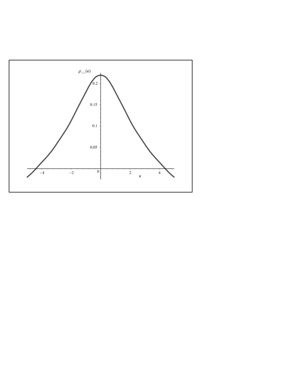
Figure 1: Plot of the finite part of the spectral density $\rho_{\text{fin}}^{2L}(\kappa)$ computed at the level $L=62$. $\rho_{\text{fin}}(0)=\frac{\log 2}{\pi}$.

The integral in the r.h.s. of (5.8) converges rather quickly and can be easily computed numerically. We compute this integral on the interval $(-30,30)$ for several values of $L$ (see Table 1). All this values are in a good agrement this the interpolating formula $a+b/\log L$.

$L$	$32$	$52$	$62$	$82$	$\infty$
$\int$	$-0.03550$	$-0.03558$	$-0.03561$	$-0.03563$	$-0.03602$

Table 1: Here we present the numeric values of the quickly convergent integral $\int_{-\infty}^{\infty}d\kappa\,\rho_{\text{fin}}^{2L}(\kappa)\log\bigl{(}1-\mu^{2}\bigr{)}$ computed at level $L$. In the very right column we present the value for this integral estimated by the formula $a+b/\log L$.

The finite part of the exponent in (5.5) can be computed by summing up residues in the upper half plane

$$(\text{finite})=\frac{\epsilon Q^{2}}{4}\,\left(-\frac{1}{2}V_{0n}^{\prime 11}\left([1-V^{\prime 11}]^{-1}\right)_{nm}J_{m}-\sum_{n,m}V_{0n}^{\prime 11}\left([1-(V^{\prime 11})^{2}]^{-1}V^{\prime 11}\right)_{nm}V_{0m}^{\prime 11}\right)\\ =\frac{\epsilon Q^{2}}{12}\int_{-\infty}^{\infty}\frac{d\kappa}{\mathcal{N}(\kappa)}\frac{2}{\kappa^{2}}\frac{1+3\mu}{1-\mu}\left[\frac{1}{2}-\frac{1}{3}\frac{1+3\mu}{1+\mu}\mu\right]\\ =-\frac{\epsilon Q^{2}}{3}\log\gamma-\frac{\epsilon Q^{2}}{36}\left[\log 4+\frac{7}{2\pi^{2}}\zeta(3)\right].$$ (5.10)

If we substitute all of our results (5.8), (5.10) into equation (5.5) we obtain

$$\log\,\langle f^{(3)}_{1},-Q|I\circ f^{(3)}_{1}\circ I,0\rangle=\lim_{L\to\infty}\left(\frac{D+1}{72}-\frac{\epsilon Q^{2}}{24}\right)\sum_{n=1}^{L}\frac{1}{n}\\ -\frac{D+1}{2}\int_{-\infty}^{\infty}d\kappa\,\rho_{\text{fin}}^{2L}(\kappa)\log(1-\mu^{2})-\frac{\epsilon Q^{2}}{3}\log\gamma-\frac{\epsilon Q^{2}}{36}\left[\log 4+\frac{7}{2\pi^{2}}\zeta(3)\right]$$ (5.11)

where for completeness we wrote both divergent and finite parts. As already noted the divergent parts cancel out for $Q=-3$, $D=26$, $\epsilon=1$. The value of the finite part can be estimated using the results presented in Table 1. It turns out to be close to the number $0.81805$ that seams to be far from the wanted $0$. We hope that the origin of this difference is just an artifact of our numeric calculations. An analytic expression for the finite part of the spectral density would certainly come handy in proving the exact identity (5.2).

6 Continuous Moyal versus Witten’s star product

6.1 Normalization of the multiplication kernel

The total multiplication kernel combining the matter and ghost sectors contains an overall normalization constant

$$\mathscr{K}_{Q=0}^{D}\mathscr{K}_{Q}=\det\Bigl{[}\frac{2}{\theta^{2}(\kappa)}\Bigr{]}^{D+1}\times\det\Bigl{[}\frac{12+\theta^{2}(\kappa)}{16}\Bigr{]}^{D+1}\exp\Bigl{[}\epsilon\frac{Q^{2}}{24}\sum_{n=1}^{\infty}J_{n}^{2}-\epsilon\frac{Q^{2}}{3}\log\gamma\Bigr{]}\,.$$ (6.1)

We can now apply the regularization technique of the previous section to compute this constant. We will keep the first factor untouched for the reason to be discussed a little later. The divergent part contained in the second two factors reads

$$\exp\left[\left(\frac{D+1}{2\pi}\int_{0}^{\infty}d\kappa\,\log\left(\frac{12+\theta^{2}(\kappa)}{16}\right)+\frac{\epsilon Q^{2}}{24}\right)\sum_{n=1}^{L}\frac{1}{n}\right]=\exp\left[\left(-\frac{D+1}{18}+\frac{\epsilon Q^{2}}{24}\right)\sum_{n=1}^{L}\frac{1}{n}\right]$$ (6.2)

and we see that for the parameters corresponding to the critical bosonic string these infinities do not cancel each other. This agrees with an analogous computation made in [16]. In this calculations we use

$$\int_{0}^{\infty}d\kappa\,\log\left(\frac{12+\theta^{2}(\kappa)}{16}\right)=-\frac{\pi}{9}.$$

We must note here that there is a potential subtlety in the above computation having to do with the finite part of the spectral density. It contributes the exponent

$$\exp\Bigl{[}(D+1)\int_{0}^{\infty}d\kappa\,\rho_{\text{fin}}(\kappa)\log\left(\frac{16}{12+\theta^{2}(\kappa)}\right)\Bigr{]}$$

which we attributed to the finite part. Strictly speaking we do not know the asymptotics of the function $\rho_{\text{fin}}(\kappa)$ as $\kappa$ goes to infinity. However given the fact that it is being integrated with a factor that is exponentially falling off at infinity it looks unlikely that the integral diverges. We hope to clarify this subtlety in a future work.

6.2 Relation between continuous Moyal and string products

In this section we will try to state clearly the precise correspondence between Witten’s and continuous Moyal star products. We start by reminding that the Moyal product of two functions on $\mathbb{R}^{2}$ can be defined by a kernel $K_{\theta}(x_{1},x_{2},x_{3})$ in the following way

$$(f\star g)(x_{1})=\int_{\mathbb{R}^{2}}dx_{2}dx_{3}\,K_{\theta}(x_{1},x_{2},x_{3})f(x_{2})g(x_{3}),$$ (6.3a)

where

$$K_{\theta}(x_{1},x_{2},x_{3})=\frac{1}{\pi^{2}\theta^{2}}\,\exp\left[-\frac{2i}{\theta}\epsilon_{\alpha\beta}\Bigl{(}x_{1}^{\alpha}x_{2}^{\beta}+x_{2}^{\alpha}x_{3}^{\beta}+x_{3}^{\alpha}x_{1}^{\beta}\Bigr{)}\right]$$ (6.3b)

$\theta$ is a real deformation parameter and matrix $\epsilon_{\alpha\beta}$ is defined in (3.10c). Notice that one needs the factor $\theta^{-2}$ in the kernel to obtain a kernel for pointwise multiplication in the limit $\theta\to 0$.

The continuous Moyal product will be defined as a product of functionals $\mathscr{F}[X^{\alpha,\mu}(\kappa)]$, where the functions $X^{\alpha,\mu}(\kappa):\mathbb{R}_{+}\to\mathbb{R}^{2}\otimes\mathbb{R}^{D}$ ($\alpha=e,o$ and $\mu=0,\dots,D-1$) will be considered as canonical coordinates on our non-commutative space. Then the product can be defined as follows

$$(\mathscr{F}_{1}\ast\mathscr{F}_{2})[X^{(3)}]=\int\mathscr{D}X^{(1)}\mathscr{D}X^{(2)}\,K_{\text{Moyal}}\bigl{(}X^{(1)},X^{(2)},X^{(3)}\bigr{)}\mathscr{F}_{1}[X^{(1)}]\mathscr{F}_{2}[X^{(2)}],$$ (6.4a)

where the measure $$\mathscr{D}X K_{\text{Moyal}}$$ is defined in (4.5) and the continuous Moyal kernel is of the form

$$K_{\text{Moyal}}\bigl{(}X^{(1)},X^{(2)},X^{(3)})=\det\bigl{[}\theta(\kappa)\bigr{]}^{-2D}\exp\left[2i\int_{0}^{\infty}\frac{d\kappa}{\theta(\kappa)}\,\sum_{\mu=0}^{D-1}x_{e,\mu}^{(r)}(\kappa)\chi^{rs}x_{o,\mu}^{(s)}(\kappa)\right].$$ (6.4b)

Here the determinant should be understood as in (5.6b). We also include in this definition a normalization factor $\det\bigl{[}\theta(\kappa)\bigr{]}^{-2D}$. Despite the fact that it is an infinite quantity this factor is needed to obtain a correct limit as $\kappa\to 0$, when we get a commutative mode. One might think that the kernels (6.4b) and (6.3b) differ due to the factor $\pi^{2}$, but actually this difference is only because of the difference in the measure normalization we use in (6.4a) and (6.3a).

The combined multiplication kernel that we obtained differs from (6.4b) by a linear exponent factor present in the ghost kernel (4.9a) and by an additional normalization factor $\mathcal{C}$:

$$\mathcal{C}=\frac{\mathscr{K}_{Q=0}^{D}\mathscr{K}_{Q}}{\det\bigl{[}\theta(\kappa)\bigr{]}^{-2(D+1)}}=\det\left[2\cdot\frac{12+\theta^{2}(\kappa)}{16}\right]^{D+1}\exp\left[-\frac{\epsilon Q^{2}}{24}\sum_{n=1}^{\infty}J_{n}^{2}+\frac{\epsilon Q^{2}}{3}\log\gamma\right]$$ (6.5)

Our results can therefore by summarized in the following mapping establishing an isomorphism of algebras

$${\cal I}:\mathcal{C}^{-1}\cdot\exp\left[-i\sqrt{2}\epsilon\Bigl{(}q+\frac{Q}{2}\Bigr{)}\int_{0}^{\infty}d\kappa\,J_{\kappa}x_{e}(\kappa)\right]\Psi_{q}[X]\quad\mapsto\quad\mathscr{F}_{q}[X],$$ (6.6)

that is ${\cal I}$ specifies a field redefinition that maps the Witten star product into the canonically normalized continuous Moyal product (6.4b). In view of the investigations made in the previous sections the redefinition involves an infinite multiplicative factor (same problem was noted in the matter sector in [5]). We could in principle remove this factor from the kernel and hide it into the $\mathscr{D}X$ functional integration measure, but then it would show up again in front of normalized wave functionals, like the one representing the vacuum state. We are not sure though at the current stage of investigation whether this infinite factor is a serious drawback of the continuous Moyal formalism in SFT. One should be able to do computations keeping these factors regulated and finite.

7 Conclusions

Here we summarize the main results of the paper.

We diagonalized the $3$-string vertex for a general bosonized Bose/Fermi ghost system (see (3.9)). Our results can be easily generalized for the non-zero momentum matter sector (see Appendix D). In the diagonal basis the string star product was rewritten in a mixed coordinate/momentum representation and expressions for the kernel and its normalization constant (see (4.9)) were obtained. We showed that this kernel defines an associative multiplication. In particular our computations reveal that the correct midpoint insertion operator is necessary for the associativity.

One of the side issues considered along the way was a non-perturbative proof of the statement that the $\mathop{\mathrm{bpz}}\nolimits$ inner product of any two surface states (with appropriate ghost insertions) is equal to one in CFT with vanishing central charge. We considered in detail the computation of an overlap of the wedge state $|0\rangle\star|0\rangle$ with itself. It was shown that for the critical bosonic string this inner product is finite. We also discussed calculation of finite parts in the identity.

The main issue considered in the paper is an isomorphism between the Witten star product algebra and a canonically normalized continuous Moyal algebra. An explicit expression for the constant relating these to algebras was found (6.5). Modulo some potential subtleties having to do with the finite part of spectral density this constant appears to be divergent.

One of the unsolved problems among others discussed in this paper is to obtain an analytic expression for the finite part of the spectral density (5.7).

Appendix

Appendix A Relations involving vector $J_{n}$

The generating function for the vector $J_{n}$ can be obtained directly from the expression (2.5e) and is of the form

$$J(z)=\sum_{n=1}^{\infty}J_{n}\frac{z^{n}}{\sqrt{n}}=-\frac{1}{\sqrt{2}}\log(1+z^{2}).$$ (A.1)

Now comparing this function with the generating function (B.26) from [6] and using the expressions (3.17a) and (B.21) from [6] one can obtain the following representation for the vector $J$

$$J=-\mathscr{P}\frac{1}{C^{\prime}U^{\prime}+1}W.$$ (A.2)

Notice also that vector $J$ is an even one

$$C^{\prime}J=J.$$ (A.3)

Using the representation (A.2) one can obtain the following useful relations involving vector $J$

$$U^{\prime}J =-\bar{W}-J$$ (A.4a)

$$\bar{U}^{\prime}J =-W-J;$$ (A.4b)

We also need to know the inner product of $J$ with $W$

$$\sum_{n=1}^{\infty}W_{n}J_{n}=\sum_{n=1}^{\infty}\bar{W}_{n}J_{n}=-V_{00}^{\prime}.$$ (A.5)

This relation can be obtained using diagonal representation of $J$ and $W$

$$\sum_{n=1}^{\infty}W_{n}J_{n}=-\int_{-\infty}^{\infty}\frac{d\kappa}{\mathcal{N}(\kappa)}\,\frac{2}{\kappa^{2}}(1+\nu(\kappa))\equiv-\int_{-\infty}^{\infty}\frac{d\kappa}{\kappa^{2}\mathcal{N}(\kappa)}\,\bigl{[}2+\nu(\kappa)+\bar{\nu}(\kappa)\bigr{]}\\ =-2\int_{0}^{\infty}\frac{d\kappa}{\kappa^{2}\mathcal{N}(\kappa)}\,\bigl{[}1+3\mu(\kappa)\bigr{]}=-V_{00}^{\prime}$$ (A.6)

Appendix B Diagonalization of $3$-string vertex

Let us rewrite the terms appearing in the exponential (2.5a) in the basis $e_{\kappa}^{{\dagger}}$, $o_{\kappa}^{{\dagger}}$. The quadratic part gets the following from in the diagonal basis

$$\sum_{r,s}\sum_{n,m=1}^{\infty}a_{n}^{(r){\dagger}}V_{nm}^{\prime\,rs}a_{m}^{(s){\dagger}}=\int_{-\infty}^{\infty}d\kappa\,C^{\prime}a_{\kappa}^{(r){\dagger}}\mu^{rs}(\kappa)a_{\kappa}^{(s){\dagger}}=\int_{0}^{\infty}d\kappa\,a_{\kappa,\alpha}^{(r){\dagger}}V^{rs}{}_{\alpha\beta}a_{\kappa,\beta}^{(s){\dagger}},$$ (B.1a)

where $$a_{\kappa,\alpha}^{{\dagger}}=(e_{\kappa}^{{\dagger}},o_{\kappa}^{{\dagger}})_{\alpha}$$ and

$$V^{rs}{}_{\alpha\beta} =\mu\delta_{\alpha\beta}\otimes\delta^{rs}+\mu_{s}\delta_{\alpha\beta}\otimes\varepsilon^{rs}+i\mu_{a}\epsilon_{\alpha\beta}\otimes\chi^{rs};$$ (B.1b)

$$\mu =\mu^{11}=\frac{-1+t^{2}}{3+t^{2}},\qquad\mu_{s}=\frac{1}{2}(\mu^{12}+\mu^{21})=\frac{2}{3+t^{2}}$$ (B.1c)

$$\mu_{a} =\frac{1}{2}(\mu^{12}-\mu^{21})=\frac{2t}{3+t^{2}},\qquad t=\tanh\frac{\pi\kappa}{4}.$$ (B.1d)

The matrices $\epsilon_{\alpha\beta}$, $\varepsilon^{rs}$ and $\chi^{rs}$ are defined in (3.10c).

The part linear in $a_{n}$ and $q$ gets the form

$$\sum_{r,s}\sum_{n=1}^{\infty}q^{(r)}V_{0n}^{\prime\,rs}a_{n}^{(s){\dagger}}=-\frac{\sqrt{2}}{3}\int_{-\infty}^{\infty}\frac{d\kappa}{\kappa\sqrt{\mathcal{N}(\kappa)}}q^{(r)}\Bigl{(}3\delta^{rs}-2+3\mu^{rs}\Bigr{)}a_{\kappa}^{(s){\dagger}}\\ =\int_{0}^{\infty}\frac{d\kappa}{\kappa\sqrt{\mathcal{N}(\kappa)}}\left[-(1+3\mu)\Bigl{(}q^{(r)}+\frac{Q}{3}\Bigr{)}e_{\kappa}^{(s){\dagger}}-2i\mu_{a}q^{(r)}\chi^{rs}o_{\kappa}^{(s){\dagger}}\right]\\ =\int_{0}^{\infty}\frac{d\kappa}{\kappa\sqrt{\mathcal{N}(\kappa)}}\,2\mu_{a}\left[-t\Bigl{(}q^{(r)}+\frac{Q}{3}\Bigr{)}e_{\kappa}^{(s){\dagger}}-iq^{(r)}\chi^{rs}o_{\kappa}^{(s){\dagger}}\right]$$ (B.2)

The term corresponding to the midpoint insertion has the following form in the diagonal basis

$$\sum_{n=1}^{\infty}J_{n}a_{n}^{(r){\dagger}}=\sqrt{2}\int_{-\infty}^{\infty}\frac{d\kappa}{\kappa\sqrt{\mathcal{N}(\kappa)}}\,a_{\kappa}^{(r){\dagger}}\stackrel{{\scriptstyle\ref{ae}}}{{=}}2\int_{0}^{\infty}\frac{d\kappa}{\kappa\sqrt{\mathcal{N}(\kappa)}}\,e_{\kappa}^{(r){\dagger}}.$$ (B.3)

The divergent term reads

$$\sum_{n=1}^{\infty}J_{n}^{2}=\int_{-\infty}^{\infty}\frac{d\kappa}{\mathcal{N}(\kappa)}\,(v^{(\kappa)},J)^{2}=2\int_{-\infty}^{\infty}\frac{d\kappa}{\kappa^{2}\mathcal{N}(\kappa)}=2\int_{0}^{\infty}d\kappa\,J_{\kappa}^{2},$$ (B.4)

where $J_{\kappa}$ is defined by (3.10g)

The term that depends only on the momentum can be rewritten in the integral representation using expression (A.6)

$$V_{00}^{\prime}\left(\sum_{r}q_{r}^{2}-Q^{3}\right)=\int_{0}^{\infty}d\kappa\,J_{\kappa}^{2}(1+3\mu)\left(\sum_{r}q_{r}^{2}-Q^{2}\right).$$ (B.5)

Appendix C Calculations of the kernel

For simplicity we will calculate the kernel $K$ in basis (4.1) for fixed $\kappa$. This means that we will drop integration over $\kappa$ in the proceeding calculations. The kernel defining multiplication in the coordinate representation has the following form (we assume $\sum_{r}q_{r}+Q=0$)

$$K_{\{q_{r}\}}(X^{(1)},X^{(2)},X^{(3)})=\bigl{(}\langle X^{(1)}_{\kappa}|\otimes\langle X^{(2)}_{\kappa}|\otimes\langle X^{(3)}_{\kappa}|\bigr{)}|V_{3}\rangle\\ =\int\mathscr{D}a\mathscr{D}a^{*}\,\exp\left[-\frac{\epsilon}{2}\begin{pmatrix}a&a^{*}\end{pmatrix}\begin{pmatrix}-1&1\\ 1&V\end{pmatrix}\begin{pmatrix}a\\ a^{*}\end{pmatrix}-\epsilon\begin{pmatrix}-i\sqrt{2}x&\Phi\end{pmatrix}\begin{pmatrix}a\\ a^{*}\end{pmatrix}\right]\\ \times\exp\left[-\frac{\epsilon}{2}\sum_{r}(x^{(r)},x^{(r)})-\frac{\epsilon}{4}J_{\kappa}^{2}(1+3\mu)\Bigl{(}\sum_{r}q_{r}^{2}-Q^{2}\Bigr{)}\right]\\ =\det{}^{-1/2}(1+V)\exp\left[\frac{\epsilon}{2}\begin{pmatrix}-i\sqrt{2}x&\Phi\end{pmatrix}\begin{pmatrix}-1&1\\ 1&V\end{pmatrix}^{-1}\begin{pmatrix}-i\sqrt{2}x\\ \Phi\end{pmatrix}\right]\\ \times\exp\left[-\frac{\epsilon}{2}\sum_{r}(x^{(r)},x^{(r)})-\frac{\epsilon}{4}J_{\kappa}^{2}(1+3\mu)\Bigl{(}\sum_{r}q_{r}^{2}-Q^{2}\Bigr{)}\right]$$ (C.1)

Notice that

$$\begin{pmatrix}-1&1\\ 1&V\end{pmatrix}^{-1}=(1+V)^{-1}\begin{pmatrix}1&1\\ 1&1\end{pmatrix}+\begin{pmatrix}-1&0\\ 0&0\end{pmatrix}$$

and

$$(1+V)^{-1}=\frac{1}{2}\otimes 1-\frac{i}{2t}\epsilon\otimes\chi.$$ (C.2)

Substitution yields the following expression for the kernel

$$K_{\{q_{r}\}}(x^{(1)},x^{(2)},x^{(3)})=\det{}^{-1/2}(1+V)\exp\left[\frac{\epsilon}{2}\sum_{r}(x^{(r)},x^{(r)})-\epsilon\,x(1+V)^{-1}x\right.\\ \left.-i\epsilon\sqrt{2}\,x(1+V)^{-1}\Phi+\frac{\epsilon}{2}\Phi(1+V)^{-1}\Phi\ -\frac{\epsilon}{4}J_{\kappa}^{2}(1+3\mu)\Bigl{(}\sum_{r}q_{r}^{2}-Q^{2}\Bigr{)}\right]$$ (C.3)

We further obtain

the $$xx$$-term:

$$x(1+V)^{-1}x=\frac{1}{2}\sum_{r}(x^{(r)},x^{(r)})-\frac{i}{t}\Bigl{(}x^{(1)}\wedge x^{(2)}+x^{(2)}\wedge x^{(3)}+x^{(3)}\wedge x^{(1)}\Bigr{)}\,,$$ (C.4a)

the $$x\Phi$$-term:

$$\sqrt{2}\,x(1+V)^{-1}\Phi=\frac{1}{\sqrt{2}}\sum_{r}\left(x_{e}^{(r)}\Phi_{e}^{(r)}+x_{o}^{(r)}\Phi_{o}^{(r)}\right)-\frac{1}{\sqrt{2}}\frac{i}{t}\left(\Phi_{e}^{(r)}\chi^{rs}x_{o}^{(s)}-\Phi_{o}^{(r)}\chi^{rs}x_{e}^{(s)}\right)\\ \stackrel{{\scriptstyle\ref{Phioe}}}{{=}}\frac{1}{\sqrt{2}}\left[x_{e}^{(r)}\Phi_{e}^{(r)}+\frac{i}{t}\Phi_{o}^{(r)}\chi^{rs}x_{e}^{(s)}\right]=\sqrt{2}J_{\kappa}\sum_{r}x_{e}^{(r)}\Bigl{(}q^{(r)}+\frac{Q}{2}\Bigr{)}\,,$$ (C.4b)

the $$\Phi\Phi$$-term:

$$\Phi(1+V)^{-1}\Phi=\frac{1}{2}\Bigl{(}\Phi_{e}^{(r)}\Phi_{e}^{(r)}+\Phi_{o}^{(r)}\Phi_{o}^{(r)}\Bigr{)}-\frac{i}{t}\Phi_{e}^{(r)}\chi^{rs}\Phi_{o}^{(s)}\\ \stackrel{{\scriptstyle\ref{Phioe}}}{{=}}\frac{1}{2}\Bigl{(}\Phi_{e}^{(r)}\Phi_{e}^{(r)}-\Phi_{o}^{(r)}\Phi_{o}^{(r)}\Bigr{)}=\frac{1}{2}J_{\kappa}^{2}(1+3\mu)\left[\sum_{r}q_{r}^{2}-\frac{Q^{2}}{3}\right]+\frac{Q^{2}}{6}J_{\kappa}^{2}$$ (C.4c)

while the determinant reads

$$\det(1+V)^{-1}=\det(\frac{1}{2}\otimes 1-\frac{i}{2t}\epsilon\otimes\chi)=\frac{1}{2^{6}}\det\left[1\otimes 1-\frac{i}{t}\epsilon\otimes\chi\right]\,.$$ (C.4d)

We used the following trick to calculate the determinant:

$$\log\det\left[1\otimes 1-\frac{i}{t}\epsilon\otimes\chi\right]=\mathop{\mathrm{Tr}}\nolimits\log\left[1\otimes 1-\frac{i}{t}\epsilon\otimes\chi\right]=-\mathop{\mathrm{Tr}}\nolimits\sum_{n=1}^{\infty}\frac{(-1)^{n}}{n}\frac{(-i)^{n}}{t^{n}}\epsilon^{n}\otimes\chi^{n}\\ =-\sum_{n=1}^{\infty}\frac{1}{n}\,t^{-2n}\mathop{\mathrm{Tr}}\nolimits\chi^{2n}=-\sum_{n=1}^{\infty}\frac{1}{n}\,t^{-2n}(-3)^{n-1}(-2\cdot 3)=2\log\left[1+\frac{3}{t^{2}}\right]$$ (C.4e)

To obtain this we use $$\chi^{2n}=(-3)^{n-1}(\varepsilon-2) \epsilon^{2n}=(-1)^{n}\mathbf{1}_{2}$$, . Combining equations (C.4d) and (C.4e) one obtains the following formula for the determinant

$$\det(1+V)=4\left(\frac{4t^{2}}{t^{2}+3}\right)^{2}\equiv 4(1+3\mu)^{2}$$ (C.4f)

Substitution of (C.4) into (C.3) yields

$$K_{\{q_{r}\}}(x^{(r)})=\frac{1}{2(1+3\mu)}\exp\left[\frac{i\epsilon}{t}\Bigl{(}x^{(1)}\wedge x^{(2)}+x^{(2)}\wedge x^{(3)}+x^{(3)}\wedge x^{(1)}\Bigr{)}\right.\\ \left.-2i\epsilon\lambda_{\kappa}\sum_{r}x_{e}^{(r)}\Bigl{(}q^{(r)}+\frac{Q}{2}\Bigr{)}+\left(\frac{\epsilon Q^{2}}{24}\sum_{n=1}^{\infty}J_{n}^{2}-\frac{\epsilon Q^{2}}{3}\log\gamma\right)\right]$$

Appendix D Non-zero momentum matter $3$-string vertex

The aim of this appendix is to adapt the formulae obtained in Sections 3 and 4 to the non-zero momentum $3$-string matter vertex. Essentially all we need to do is to put $Q=0$, substitute $p_{r}=-q_{r}$, change the Kronecker symbol to the Dirac delta function, change all sums to the integrals and substitute $\epsilon\mapsto g_{\mu\nu}$.

The matter $3$-string vertex in the diagonal basis has the following form

$$|V_{3}^{(\text{matter})}\rangle_{123}=\frac{1}{(2\pi)^{\frac{D}{2}}}\int d^{D}p^{(1)}d^{D}p^{(2)}d^{D}p^{(3)}\,(\deg g)^{-1}\delta(p^{(1)}+p^{(2)}+p^{(3)})\\ \times\exp\left[\int_{0}^{\infty}d\kappa\left(-\frac{1}{4}J_{\kappa}^{2}(1+3\mu)p^{(r)}_{\mu}g^{\mu\nu}p^{(r)}_{\nu}\Bigr{]}\right.\right.\\ \left.\left.-\sum_{r}\Phi^{(r)}_{\alpha,\mu}(\kappa)g^{\mu\nu}a_{\kappa,\alpha,\mu}^{(r){\dagger}}-\frac{1}{2}g^{\mu\nu}a_{\kappa,\alpha,\mu}^{(r){\dagger}}V^{rs}_{\kappa,\alpha\beta}a_{\kappa,\beta,\nu}^{(s){\dagger}}\right)\right]\bigotimes_{r=1}^{3}|p^{(r)}\rangle,$$ (D.1)

where $V_{\kappa,\alpha\beta}^{rs}$ is the same as for the ghost part and

$$\Phi_{e,\mu}^{(r)}(\kappa) =-\frac{1}{2}J_{\kappa}(1+3\mu)p^{(r)}_{\mu},$$ (D.2)

$$\Phi_{o,\mu}^{(r)}(\kappa) =-iJ_{\kappa}\mu_{a}p^{(s)}_{\mu}\chi^{sr}\equiv\frac{2i}{\theta(\kappa)}\,\Phi_{e}^{(s)}\chi^{sr}.$$ (D.3)

The multiplication kernel in the mixed coordinate/momentum basis has the form

$$K_{\{p_{1},p_{2}\}}(X^{(r)})\equiv\Bigl{(}\langle X^{(1)},p_{1}|\otimes\langle X^{(2)},p_{2}|\otimes\langle X^{(3)},-p_{1}-p_{2}|\Bigr{)}|V_{3}\rangle\\ =\mathscr{K}_{Q=0}^{D}\exp\left[2i\int_{0}^{\infty}\frac{d\kappa}{\theta(\kappa)}\,g^{\mu\nu}x^{(r)}_{e,\mu}(\kappa)\chi^{rs}x^{(s)}_{o,\nu}(\kappa)\right]\times\\ \exp\left[i\sqrt{2}\int_{0}^{\infty}d\kappa\,J_{\kappa}\Bigl{\{}x_{e,\mu}^{(1)}(\kappa)p_{1}^{\mu}+x_{e,\mu}^{(2)}(\kappa)p_{2}^{\mu}-x_{e,\mu}^{(3)}(\kappa)\bar{p}_{3}^{\mu}\Bigr{\}}\right]$$ (D.4)

where $\bar{p}_{3}=p_{1}+p_{2}$.

References

• [1] E. Witten, “Noncommutative Geometry And String Field Theory,” Nucl. Phys. B 268, 253 (1986).
• [2] I. Bars, Map of Witten’s * to Moyal’s *, Phys. Lett. B 517, 436 (2001), hep-th/0106157.
• [3] I. Bars and Y. Matsuo,Associativity anomaly in string field theory, hep-th/0202030.
• [4] L. Rastelli, A. Sen, B. Zwiebach, Star Algebra Spectroscopy, hep-th/0111281
• [5] M. Douglas, H. Liu, G. Moore and B. Zwiebach, Open String Star as a Continuous Moyal Product, hep-th/0202087
• [6] D. Belov, Diagonal representation of open string star and Moyal product, hep-th/0204164.
• [7] A. Connes, Noncommutative Geometry, Academic press, New York, 1994.
• [8] M. R. Douglas and N. Nekrasov, Noncommutative Field Theory, Rev. Mod. Phys. 73 (2001) 977-1029; hep-th/0106048.
• [9] A. Konechny and A. Schwarz, Introduction to M(atrix) Theory and Noncommutative Geometry, Phys.Rept. 360 (2002) 353-465; hep-th/0107251.
• [10] I.Ya. Aref’eva, D.M. Belov, A.A. Giryavets, A.S. Koshelev, P.B. Medvedev, Noncommutative Field Theories and (Super)String Field Theories, hep-th/0111208.
• [11] K. Ohmori, A Review on Tachyon Condensation in Open String Field Theories, hep-th/0102085.
• [12] P. De Smet, Tachyon Condensation: Calculations in String Field Theory , hep-th/0109182.
• [13] R. Gopakumar, S. Minwalla and A. Strominger, Noncommutative Solitons, JHEP 0005 (2000) 020; hep-th/0003160.
• [14] V. A. Kostelecky and R. Potting, Analytical construction of a nonperturbative vacuum for open bosonic string, Phys.Rev. D63 (2001) 046007; hep-th/0008252.
• [15] B. Chen and F.-L. Lin, D-branes as GMS solitons in Vacuum String Field Theory, hep-th/0204233.
• [16] T.G. Erler, Moyal Formulation of Witten’s Star Product in the Fermionic Ghost Sector, hep-th/0205107
• [17] I.Ya. Aref’eva, A.A. Giryavets, Open Superstring Star as a Continuous Moyal Product, hep-th/0204239
I.Ya. Aref’eva, A.A. Giryavets and A.S. Koshelev, NS Ghost Slivers, hep-th/0203227
• [18] D. Friedan, E. Martinec, and S. Shenker, Conformal Invariance, Supersymmetry, and String Theory, Nucl.Phys. B271 (1986) 93.
• [19] D. Friedan, Notice on String Theory and Two Dimensional Conformal Field Theory’ preprint EFI 85-99 (1986).
• [20] D. Gross, A. Jevicki, Operator Formulation of Interacting String Field Theory (I), Nucl.Phys. B283 (1987) 1 – 49
• [21] A. Le Clair, M. Peskin and C. Preitschopf, String field theory on the conformal plane (I). Kinematical principles, Nucl. Phys. B317 (1989) 411-463.
• [22] L. Rastelli, A. Sen, B. Zwiebach, Classical Solutions in String Field Theory Around the Tachyon Vacuum, hep-th/0102112
• [23] A. Le Clair, M. Peskin and C. Preitschopf String field theory on the conformal plane (II). Generalized gluing, Nucl. Phys. B317 (1989) 464.
• [24] A. Jevicki, Construction Of Interacting String and Superstring Field Theory, Int. J. Mod. Phys. A 3, 299 (1988).
• [25] K. Okuyama, Ghost Kinetic Operator of Vacuum String Field Theory, hep-th/0201015
• [26] A. Schwarz and A. Sen, Gluing theorem, star product and integration in open string field theory in arbitrary background fields, Int. Jr. of Modern Physics A, Vol. 6, No. 30 (1991) 5387-5407.
• [27] L. Rastelli and B. Zwiebach, Tachyon potentials, star products and universality, hep-th/0006240.
• [28] L. Rastelli, A. Sen and B. Zwiebach, JHEP 0111, 045 (2001) [arXiv:hep-th/0105168].
• [29] I. Bars and Y. Matsuo,Computing in string field theory using the Moyal star product, hep-th/0204260.
• [30] A. Sen, Stable non BPS bound states of bps d-branes, JHEP 08, 010 (1998), hep-th/9805019
A. Sen, SO(32) spinors of type i and other solitons on brane - anti-brane pair, JHEP 09, 023 (1998), hep-th/9808141
• [31] D. Gross, A. Jevicki, Operator Formulation of Interacting String Field Theory (II), Nucl.Phys. B287 (1987) 225 – 250
• [32] K. Okuyama, Ratio of Tensions from Vacuum String Field Theory, hep-th/0201136
• [33] F.A. Berezin, The method of second quantization, New York, Academic Press, 1966