CU-TP-1064 ,HWS-200201 ,HU-EP-02/28 
hep-th/0207162
Intersecting Branes in M-Theory
and Chiral Matter in Four Dimensions

We explicitly derive a complementary pair of four-dimensional M-theory brane-world models, linked by a five-dimensional bulk, each of which has a unique anomaly-free chiral spectrum. This is done via resolution of local consistency requirements, in the context of the simplest global quotient $T^{7}/\Gamma$ involving ten-dimensional fixed-planes, for which a chiral four-dimensional spectrum could arise.

1 Introduction

One of the preeminent tasks of contemporary theoretical physics is to seek a mathematically consistent higher-dimensional explanation for the chiral fermion spectrum and gauge symmetries of the standard model. Over the last decade, string theory has precipitated a virtual miasma of related ideas. Recently, two different sorts of constructions have emerged as compelling avenues for the derivation of effective physics from within both string theory and also its elusive non-perturbative cousin, M-theory. On the one hand, brane-world models [1, 2, 3, 4], obtained by consistent inclusion of intersecting D-branes and open strings in various background geometries [5, 6], have succeeded in providing a plausible context for the standard model itself [7, 8, 9, 10]. On the other hand, M-theory has inspired a search for a more elegant eleven-dimensional underpinning to some of these same constructions, and has stimulated an interest in the physically-relevant mathematical characterization of $G_{2}$ holonomy seven-manifolds [11, 12].

There are two essential obstructions which have hampered the search for M-theoretic phenomenology as compared to string theory analogues. One is the fact that a fundamental description of M-theory has not yet emerged. The other is that much less is known about $G_{2}$ holonomy seven-manifolds than is known about Calabi-Yau threefolds. Thus, it is difficult to provide geometric explanations for the symmetries and spectra which may arise in M-theory compactifications. However, there is one restricted class of constructions tailor-made to shed light on each of these two problems, which also includes a built-in mechanism for resolving effective physics. This is the class of models based on global orbifold compactifications of eleven-dimensional supergravity.

One reason why orbifold compactifications are so useful in M-theory is that it is relatively simple to answer the question of how much supersymmetry is preserved on the various fixed-planes of a given orbifold, provided the action of the associated quotient group has a well-defined lift to the eleven-dimensional spinorial supercharge. It is therefore a straightforward exercise to categorize a wide class of supersymmetric orbifolds in M-theory. Presumably these singular constructions can be resolved to smooth, compact $G_{2}$ manifolds [13], and therefore provide a skeletal basis for the characterization of such spaces. Especially useful are the stringent constraints, based on local anomaly cancellation, which allow one to readily discern chiral states and additional characteristic classes (“rational bundle data”) localized on the network of fixed planes. In this way, many M-theory orbifold models are very similar to string theory brane-world constructions.

In the interest of developing a robust and useful algorithm for extracting effective physics from generic supersymmetric M-theory orbifolds, we analyze and resolve the network of constraints which follow from the necessary requirement of gauge and gravitational anomaly cancellation point-wise in eleven dimensions. Quite a bit of the necessary apparatus has been developed in preceding papers [14, 15, 16, 17]. With some care the technology described in those papers can be applied to a wide class of models. It is opportune, therefore, to investigate which orbifold constructions are especially interesting, so that we can proceed to cycle through these, model-by-model, in the interest of identifying those which have the greatest phenomenological appeal, to enable an appropriately thorough comparison with string theory models, and to learn as much as possible about the world of M-theory physics.

Considering M-theory on a spacetime with topology $\mathbb{R}^{3,1}\times X^{7}$, the preservation of $N=1$ supersymmetry requires that $X^{7}$ have $G_{2}$ holonomy [11]. Furthermore, the presence of chiral fermions and non-abelian gauge symmetries in four dimensions adds another requirement to the structure of $X^{7}$, namely, this space cannot be smooth; it must possess singularities of one sort or another [12, 18]. One constructive approach, which easily includes both the $G_{2}$ requirement and also the requirement of singularities is to focus on global orbifold constructions. In this case, we can replace the geometric holonomy constraint with the requirement that some components of the eleven-dimensional supercharge are preserved at each point. Since this can be readily implemented on global orbifolds $T^{7}/\Gamma$, rather than on merely local models of orbifold singularities (e.g., $\mathbb{R}^{7}/\Gamma$), we gain insight into the physics corresponding to global $G_{2}$ compactifications.

More generally, we would like to study all possible orbifolds $T^{7}/\Gamma$, where the torus $T^{7}$ is itself defined as a quotient $\mathbb{R}^{7}/\Lambda$, with $\Lambda$ a generic lattice in $\mathbb{R}^{7}$ and $\Gamma$ a subset of the automorphisms of $\Lambda$. It is worthwhile, however, to restrict attention to an important subset of these constructions, namely those for which $\Gamma\subset SO(7)\subset SO(10,1)$ is an abelian finite group represented by rotations in three complex planes plus the possibility of a parity flip in an additional real coordinate. In these cases each element of $\Gamma$ lifts to an action on spinors, such as the supercharge $Q$, in a manner which is especially amenable to analysis. One can thereby readily determine the set of supersymmetric orbifolds of this class.

We make one more important restriction: we limit attention to those orbifolds for which no group element acts freely on any of the coordinates of $T^{7}$. We call these hard orbifolds. In this case, each element has fixed planes associated with it, and the set of fixed planes generically intersect as an intricate tangle. Geometrically, these models are more interesting than the related cases in which $\Gamma$ includes elements with fixed-point-free “shifts” on one or more coordinates. These latter types we call soft orbifolds. One can consider the hard orbifolds as more fundamental, because each soft orbifold can be obtained from a hard orbifold by “softening” operations in which, for instance, a coordinate reflection is replaced with a shift. Geometrically, such softening operations either eliminate some of the fixed planes, or they take two fixed planes which intersect, and move them off of each other, thereby eliminating the intersection.

The number of hard abelian orbifold models which maintain supersymmetry is surprisingly restrictive. For instance, if one looks only at finite groups $\Gamma$ with order less than or equal to twelve, there are exactly $29$ such models, as depicted in Table 1.

$\Gamma$	${\rm Ord}(\Gamma)$	1	2	3	4	5	6	7
$\mathbb{Z}_{2}$	2	$1^{*}$			1	1
$\mathbb{Z}_{3}$	3				1
$\mathbb{Z}_{4}$	4				1	1	1	1
$\mathbb{Z}_{2}\times\mathbb{Z}_{2}$	4					$1^{*}$	1	1
$\mathbb{Z}_{2}\times\mathbb{Z}_{3}$	6				1	$1^{*}$+1	1	1
$\mathbb{Z}_{2}\times\mathbb{Z}_{4}$	8					$1^{*}$	$1^{*}$+1	$1^{*}$+2
$(\mathbb{Z}_{2})^{3}$	8							$1^{*}$+1
$(\mathbb{Z}_{3})^{2}$	9
$(\mathbb{Z}_{2})^{2}\times\mathbb{Z}_{3}$	12					$1^{*}$	1	$1^{*}$+2
$\mathbb{Z}_{3}\times\mathbb{Z}_{4}$	12

Table 1: A scan of supersymmetric hard abelian orbifolds of M-theory. Non-zero numbers in the table indicate the multiplicity of supersymmetric orbifolds $T^{n}/\Gamma$ for the indicated abelian finite groups. The torus dimension $n$ corresponds to the column and the quotient group $\Gamma$ correlates with the row. Stars indicate supersymmetric Horava-Witten models: those which include an isolated $S^{1}/\mathbb{Z}_{2}$ factor. Note that there are nine of these in the scan, six of which have been described previously; the simplest of the remaining three, namely the starred $T^{7}/(\mathbb{Z}_{2}\times\mathbb{Z}_{2}\times\mathbb{Z}_{3})$ model, is described in this paper.

Table 1 indicates each supersymmetric hard abelian orbifold ${\cal O}=T^{7}/\Gamma$ with ${\rm Order}(\Gamma)\leq 12$. In general, the group $\Gamma$ might act non-trivially on a subset of the seven coordinates of $T^{7}$, so that we could write instead ${\cal O}=(S^{1})^{7-n}\times T^{n}/\Gamma$. Thus, we separate the cases with distinct values of $n$, and list these in separate columns in our scan. The numbers which appear in the scan are the multiplicities of supersymmetric models $T^{n}/\Gamma$ which can be formed by representations of $\Gamma$ on an $n$-torus defined by a particular compatible lattice.

An especially interesting subset of the supersymmetric orbifold models are those which split off a separate $S^{1}/\mathbb{Z}_{2}$ factor, since these models have fixed ten-planes. We refer to such models as Hořava-Witten, or HW, models, since the most basic of these cases was first described in [19, 20]. These are interesting because local gravitational anomaly cancellation requires ten-dimensional $E_{8}$ Yang-Mills multiplets on these ten-planes. As it turns out, when these ten-planes intersect other fixed-planes, further anomaly cancellation requirements are satisfied only if the quotient group $\Gamma$ acts non-trivially on the $E_{8}$ lattices, thereby breaking these groups down to subgroups. This allows concise analytical access to information pertaining to localized rational bundle data, related to small instantons stuck on fixed-plane intersections.

In Table 1 we have indicated the HW models with an asterix. Note that there are exactly nine supersymmetric hard abelian HW models with ${\rm Order}(\Gamma)\leq 12$. The first is the basic $S^{1}/\mathbb{Z}_{2}$ model described in [19, 20]. Next are the four global orbifold limits of $K3\times S^{1}/\mathbb{Z}_{2}$, which were analyzed in [15, 16, 17, 21]. Finally, there is one five-dimensional model, wherein only six of the $T^{7}$ coordinates are influenced nontrivially by $\Gamma$, and three four-dimensional models, wherein all of the $T^{7}$ coordinates are influenced nontrivially by $\Gamma$. One of the four-dimensional models has $\Gamma=(\mathbb{Z}_{2})^{3}$, and was described in [14]. In that model, however, the four-dimensional effective physics is not chiral, a circumstance related to the fact that all the elements of the orbifold group have order two. Furthermore, that model does not have purely four-dimensional fixed-planes associated with any of the elements of $\Gamma$. For this reason, that model does not describe a true four-dimensional brane-world. Of the two remaining four-dimensional models, one has a quotient group with prime factors, and one has non-prime factors. The latter of these, corresponding to $T^{7}/(\mathbb{Z}_{2}\times\mathbb{Z}_{4})$ is relatively complicated. This is because in that case, in addition to a primary category of orbifold-planes, there is a separate subclass of hyperplanes comprising nontrivial multiplets under the subgroup $(\mathbb{Z}_{2})^{2}$. Such matters, pertaining to non-prime orbifolds were explained more comprehensively in the context of $T^{5}/\Gamma$ orbifolds in [17]. The one remaining four-dimensional HW model in our scan has $\Gamma=(\mathbb{Z}_{2})^{2}\times\mathbb{Z}_{3}$. This model has both four-dimensional fixed planes and also a chiral four-dimensional spectrum. Thus, this model is unique in that it is the simplest hard abelian orbifold with ten-dimensional fixed-planes, giving rise to a chiral four-dimensional super Yang-Mills theory.

In the bulk of this paper, we provide a microscopic anomaly analysis on the unique HW orbifold $T^{7}/(\mathbb{Z}_{2}\times\mathbb{Z}_{2}\times\mathbb{Z}_{3})$ described above. Our motivation for explaining this model in detail has less to do with the particulars of the associated four-dimensional physics than it has to do with exposing the set of techniques which we employ. Specifically, this analysis rounds out the analytical tools developed in [14, 15, 16, 17], filling in the final part of the technology: the analysis of the four dimensional gauge and mixed anomalies induced at four-dimensional fixed planes.

An interesting feature of hard orbifold models is the way in which the perceived four-dimensional gauge groups are embedded within larger groups localized on higher-dimensional planes. This in turn is governed by entwined branchings which correlate with the manner in which various orbifold planes intersect. Different branchings in this context correspond to different classes of small instantons living on the branes. In the analysis described in this paper, we do not include fivebranes. Therefore, we are describing a “basic” solution, from which additional models can be built up by the sorts of phase transitions described in [16]. This paper is structured as follows.

In section 2 we describe in detail the construction of the particular $T^{7}/(\mathbb{Z}_{2}\times\mathbb{Z}_{2}\times\mathbb{Z}_{3})$ orbifold described above. We exhibit the representation of the quotient group on the compact coordinates, and then characterize the intricate geometry of the intersecting hyper-planes invariant under elements of this group. In section 3 we explicitly derive the spectrum of states localized on each of the orbifold fixed-planes described in section 2. This analysis relies on local anomaly cancellation on each ten-, six- and four-dimensional fixed-plane in the orbifold, and involves the notion of “consistently entwined branchings”, which we define and describe. In section 4, we use the results of section 3 to determine the effective spectrum associated with complementary four-dimensional brane-worlds linked by a five-dimensional bulk, obtained by taking a “spindle” limit in which six of the compact dimensions become small. We then conclude with various observations about the relationship of M-theory models, such as the one described in this paper, with analogous constructions derived from within string theory.

2 Fixed-Plane Geometry

The simplest supersymmetric hard global orbifold of M-theory which has four-dimensional fixed-planes and a chiral four dimensional spectrum has the following structure. The eleven-dimensional spacetime has topology $\mathbb{R}^{3,1}\times T^{6}/(\mathbb{Z}_{2}\times\mathbb{Z}_{3})\times S^{1}/\mathbb{Z}_{2}$. The six-torus is defined as a lattice quotient $\mathbb{R}^{6}/\Lambda$, where $\Lambda=A_{2}\oplus A_{2}\oplus A_{1}$, and is parameterized by three complex coordinates $(\,z_{1}\,,\,z_{2}\,,\,z_{3}\,)$ . The circle $S^{1}$ is described by a real angular coordinate $x^{11}$. The quotient group $\mathbb{Z}_{2}\times\mathbb{Z}_{2}\times\mathbb{Z}_{3}$ acts on the coordinates as indicated in Table 2.

	$z_{1}$	$z_{2}$	$z_{3}$	$x^{11}$
$\alpha$	$-$	+	$-$	+
$\beta$	+	+	+	$-$
$\alpha\beta$	$-$	+	$-$	$-$
$\gamma$	1/3	$-1/3$	+	+
$\alpha\gamma$	$-1/6$	$-1/3$	$-$	+
$\beta\gamma$	1/3	$-1/3$	+	$-$
$\alpha\beta\gamma$	$-1/6$	$-1/3$	$-$	$-$

Table 2: The representation of $\Gamma=\mathbb{Z}_{2}\times\mathbb{Z}_{2}\times\mathbb{Z}_{3}$ on the coordinates of the seven torus $(\,z_{1}\,,\,z_{2}\,,\,z_{3}\,,\,x^{11}\,)$, for the orbifold described in the text. This order twelve group is generated by the elements $\alpha,\beta$ and $\gamma$. A minus sign on a complex coordinate $z_{i}$ is equivalent to an $f_{i}=1/2$ rotation. In the table we have suppressed the trivial element and the inverses of the order 3 element $\gamma$ and the three order 6 elements $\alpha\gamma$, $\beta\gamma$ and $\alpha\beta\gamma$.

In this representation, each element acts as a rotation in the three complex planes and possibly a parity flip in the $S^{1}$ direction,

$$(\,z_{1}\,,\,z_{2}\,,\,z_{3}\,,\,x^{11}\,)\rightarrow(\,e^{i\,\theta_{1}}z_{1}\,,\,e^{i\,\theta_{2}}z_{2}\,,\,e^{i\,\theta_{3}}z_{3}\,,\,(-)^{P}x^{11}\,)\,.$$ (1)

with $\theta_{i}=2\,\pi\,f_{i}$ and $P\in\{0,1\}$. Depicted in Table 2 are the fractional rotations $f_{i}$ imparted on the planes and the presence or absence of an $x^{11}$ parity flip, for each representative non-trivial element of the group. Note that the four elements $\{\,\gamma^{2}\,,\alpha\gamma^{2}\,,\,\beta\gamma^{2}\,,\,\alpha\beta\gamma^{2}\,\}$ are the respective inverses of the four elements $\{\,\gamma\,,\alpha\gamma\,,\,\beta\gamma\,,\,\alpha\beta\gamma\,\}$, and have precisely the same fixed planes. We have therefore suppressed four nontrivial elements in Table 2.

The element $\beta$ has two ten-dimensional fixed planes: an “upper” one and a “lower” one, each corresponding to a separate value of $x^{11}$. The other fixed-planes (i.e. those associated with other elements of $\Gamma$) fall into two categories: a primary set comprised of subspaces of the $\beta$-invariant ten-planes, and a secondary set involving those which span $x^{11}$. Each of the secondary fixed-planes interpolates between pairs of primary fixed planes. The primary fixed-planes are associated with the elements $\alpha\beta$, $\beta\gamma$ and $\alpha\beta\gamma$; those associated with $\alpha\beta$ and $\beta\gamma$ are six-dimensional, while those associated with $\alpha\beta\gamma$ are four-dimensional and coincide with intersections of the six-dimensional primary fixed-planes. The secondary fixed planes are associated with the elements $\alpha$, $\gamma$ and $\alpha\gamma$; those associated with $\alpha$ and $\gamma$ are seven-dimensional, while those associated with $\alpha\gamma$ are five-dimensional and coincide with intersections of the seven-dimensional secondary fixed planes. The $\alpha$-invariant seven-planes interpolate between pairs of $\alpha\beta$-invariant six-planes, the $\gamma$-invariant seven-planes interpolate between pairs of $\beta\gamma$-invariant six-planes, and the $\alpha\gamma$-invariant five-planes interpolate between $\alpha\beta\gamma$-invariant four-planes.

We first analyze the geometry of the secondary fixed-planes (i.e. those which span $x^{11}$). We are therefore interested in studying the action of $\alpha$, $\gamma$ and $\alpha\gamma$ on the three complex coordinates $(\,z_{1}\,,\,z_{2}\,,\,z_{3}\,)$, at generic values of $x^{11}$. The $\gamma$-planes are the only secondary planes which span the $z_{3}$ directions. The element $\gamma$ has order-three and acts on $(z_{1},z_{2})$, providing a set of nine ostensibly isolated $A_{2}$ orbifold singularities, each of the sort characteristic of a $\mathbb{C}^{2}/Z_{3}$ orbifold. However, at four special values of $z_{3}$ the elements $\alpha$ and $\alpha\gamma$ identify pairs of points within this set, effectively inducing intersections. At generic values of $z_{3}$ the secondary planes consist exclusively of nine $\gamma$-invariant seven-planes. At the four special values of $z_{3}$, however, the geometry is comparatively intricate.

We focus on subspaces $T^{4}\subset T^{6}$ which are spanned by $(z_{1},z_{2})$, at the four special values of $z_{3}$. The coordinates $z_{1}$ and $z_{2}$ each take values in a fundamental domain of an $A_{2}$ lattice. It is useful first to consider one such domain, that associated with $z_{1}$, which we depict as follows,

Here we have indicated special points which are fixed under relevant $\mathbb{Z}_{2}$, $\mathbb{Z}_{3}$ or $\mathbb{Z}_{6}$ actions generated by $\alpha$, $\gamma$ and $\alpha\gamma$, respectively. The origin of this complex plane is denoted $0$. The two points labelled $1$ and $2$ are $\mathbb{Z}_{3}$ invariants, but transform as doublets under $\mathbb{Z}_{2}$. The three points labelled $a$, $b$ and $c$ are $\mathbb{Z}_{2}$ invariants, but transform as a triplet under $\mathbb{Z}_{3}$. The point labelled $0$ is invariant under both $\mathbb{Z}_{2}$ and $\mathbb{Z}_{3}$ and is the only point invariant under $\mathbb{Z}_{6}$. Now consider the fundamental domain of the second $A_{2}$ lattice, that spanned by $z_{2}$. In this case, we have a picture similar to that described above, but with a crucial difference: the element $\alpha$ does not act on $z_{2}$. Thus, whereas the first $A_{2}$ lattice had only four $\alpha$-invariant points, 0, $a$, $b$ and $c$, the second $A_{2}$ lattice is $\alpha$-invariant in its entirety.

Special points in the combined $A_{2}\oplus A_{2}$ lattice parameterized by $(z_{1},z_{2})$ are represented in the obvious manner by pairs, such as $(0,0)$ or $(a,2)$. Within $(z_{1},z_{2})$, there are four parallel codimension two loci invariant under $\alpha$. These are given by $(0,z_{2})$, $(a,z_{2})$, $(b,z_{2})$ and $(c,z_{2})$, and are depicted by the green lines in Figure 1. Next, there are nine points invariant under $\gamma$. Three of these are given by $(0,0)$, $(0,1)$ and $(0,2)$, and are depicted in red in Figure 1. The other six, which comprise three doublets under $\alpha$, are given by $(1,0)\leftrightarrow(2,0)$, $(1,1)\leftrightarrow(2,1)$ and $(1,2)\leftrightarrow(2,2)$, where the arrows indicate the $\mathbb{Z}_{2}$ transformations generated by $\alpha$. (In Figure 1, these six points are depicted in blue, while the identifications corresponding to the order-two element $\alpha$ are indicated by the yellow blobs.) There are also several noteworthy $\mathbb{Z}_{3}$ identifications, as indicated in Figure 1 by the green blobs encircling triplets of grey points. For example, the three points $(0,a)$, $(0,b)$ and $(0,c)$ comprise one such $\mathbb{Z}_{3}$ triplet.

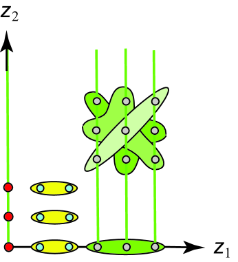
Figure 1: Points of the four-torus $(z_{1},z_{2})$ identified by the $\mathbb{Z}_{2}\times\mathbb{Z}_{3}$ subgroup of $\Gamma$ generated by $\alpha$ and $\gamma$. The red spots are the three $\mathbb{Z}_{2}\times\mathbb{Z}_{3}$ invariant points, the yellow blobs are the $\mathbb{Z}_{3}$-invariant $\mathbb{Z}_{2}$-doublets with components in blue. The green lines are the four $\mathbb{Z}_{2}$ invariants. The green blobs encircle those $\mathbb{Z}_{3}$ triplets which provide noteworthy identifications.

Thus, at the four special values of $z_{3}$, the geometry inside the $T^{4}$ parameterized by $(z_{1},z_{2})$ includes three $\mathbb{Z}_{6}$-invariant points (red) linked by a $\mathbb{Z}_{2}$-invariant complex line (green), three isolated $\mathbb{Z}_{3}$-invariant points (yellow) and four more $\mathbb{Z}_{2}$-invariant points (grey) linked by triple intersections of $\mathbb{Z}_{2}$-invariant lines (green).

Now lets consider the $z_{3}$ dependence as well, and describe the geometry inside the $T^{6}/(\mathbb{Z}_{2}\times\mathbb{Z}_{3})$ at a given value of $x^{11}$. Consider, for example, the geometry at one of the two special values of $x^{11}$ fixed by the element $\beta$, i.e. at one “end-of-the-world”. This can be depicted as shown in Figure 2.

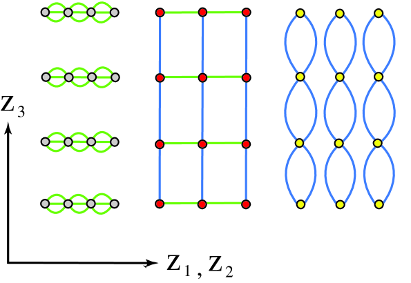
Figure 2: Fixed loci inside one of the six-tori, parameterized by $(z_{1},z_{2},z_{3})$, at one end-of-the world (i.e. at one of the two special values of $x^{11}$). The red points are the twelve $\alpha\beta\gamma$-invariant four-planes, the blue lines are the nine $\beta\gamma$-invariant six-planes, and the green lines are the sixteen $\alpha\beta$-invariant six-planes. Three of the (blue) $\beta\gamma$-invariant six-planes intersect four of the (green) $\alpha\beta$-invariant six-planes at (red) $\alpha\beta\gamma$-invariant four-planes. There are twelve such intersections. Otherwise, the six remaining (blue) $\beta\gamma$-invariant six-planes doubly intersect at the nine four-planes shown in yellow, and the twelve remaining (green) $\alpha\beta$-planes triply-intersect at the sixteen four-planes shown in grey. Six-tori at generic values of $x^{11}$ have a similar geometry.

As described previously, the only fixed planes which span $z_{3}$ are the $\beta\gamma$-invariant planes, of which there are nine. These are represented by the nine blue lines in Figure 2. At the four special values of $z_{3}$, these are identified pairwise as indicated.

Now we can describe the global geometry associated with this orbifold. At each end of the world we have the network of fixed planes shown in Figure 2. We have a similar geometry at generic values of $x^{11}$. We observe three essential sorts of extended neighborhoods. First, there are the $\mathbb{Z}_{6}$-invariant planes which each live at the intersection of one $\mathbb{Z}_{2}$-invariant plane and one $\mathbb{Z}_{3}$ invariant plane. These correspond to the red dots in Figure 2. Second, there are the triple intersections of the $\mathbb{Z}_{2}$-invariant planes, depicted in grey in Figure 2. Third, there are double intersections of $\mathbb{Z}_{3}$-invariant planes, depicted in yellow in Figure 2.

Neighborhoods of the first category extend from one $\alpha\beta\gamma$-invariant four-plane located at the intersection of an $\alpha\beta$-invariant six-plane and a $\beta\gamma$-invariant six-plane, all within one end-of-the-world (i.e. all within one $\beta$-invariant ten-plane), to a second one within the other end-of-the-world. The plane which interpolates between the two $\alpha\beta\gamma$-invariant four-planes is an $\alpha\gamma$-invariant five-plane, which lives at the intersection of an $\alpha$-invariant seven-plane and a $\gamma$-invariant seven-plane. One such extended neighborhood is depicted in the uppermost picture in Figure 3. There are twelve extended neighborhoods of the first category in this orbifold.

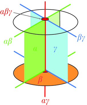
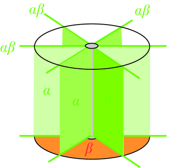
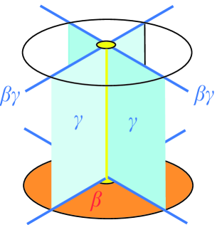
Figure 3: A local depiction showing each of the three sorts of extended neighborhoods characteristic of the orbifold described in the text. In the first instance, we exhibit two of the twelve $\alpha\beta$-invariant four-planes (red circles) connected by one of the $\alpha\gamma$-invariant five-planes (the red line). This is an extended neighborhood of the first category, as explained in the text. The lower two pictures depict extended neighborhoods of the second and third categories.

Neighborhoods of the second category extend from triple intersections, each involving three $\alpha\beta$-invariant six-planes within one end-of-the-world, to similar triple intersections within the other end-of-the-world. The planes which interpolate, spanning $x^{11}$, between pairs of the $\alpha\beta$-planes are themselves $\alpha$-invariant seven-planes. In this case the four-dimensional intersections and the five-dimensional interpolating intersection are not by-themselves invariant under any elements of the quotient group. Instead, these intersections comprise triplets under the $\mathbb{Z}_{3}$ generated by $\gamma$. One such extended neighborhood is depicted in the lower left picture in Figure 3. There are sixteen extended neighborhoods of the second category in this orbifold.

Neighborhoods of the third category extend from double intersections, each involving two $\alpha\gamma$-invariant six-planes within one end-of-the-world, to a similar double intersection within the other end-of-the-world. The planes which interpolate, spanning $x^{11}$, between pairs of the $\alpha\gamma$-planes are themselves $\gamma$-invariant seven-planes. In this case the four-dimensional intersections and the five-dimensional interpolating intersection are not by-themselves invariant under any elements of the quotient group. Instead, these intersections are triplets under the $\mathbb{Z}_{2}$ generated by $\alpha$. One such extended neighborhood is depicted in the lower right picture in Figure 3. There are twelve extended neighborhoods of the third category in this orbifold.

3 Localized States

Now that we have characterized the network of fixed planes in our orbifold, we address the issue of potential chiral anomalies localized on these planes.

The bulk gravitino field is projected chirally by the element $\beta$ onto the the $\beta$-invariant ten-planes defining the ends-of-the-world. The chiral coupling of this bulk field to currents localized on these ten-planes induces a localized gravitational anomaly. This is eliminated self-consistently (i.e. avoiding the introduction of additional gauge or mixed anonalies) by including $E_{8}$ Yang-Mills super-multiplets on each ten-plane. However, the elements $\alpha\beta$ and $\beta\gamma$ also act on the bulk gravitino field, and on the $E_{8}$ gaugino fields as well, so as to introduce additional gravitational, gauge and mixed anomalies on the six-planes associated with $\alpha\beta$ and $\beta\gamma$. These can also be eliminated self-consistently by including $SU_{2}$ and $SU_{3}$ Yang-Mills super multiplets, on the seven-dimensional $\alpha$ and $\gamma$ planes, respectively, and by adding onto the six-planes additional “twisted” hypermultiplets transforming in particular representations. But this is possible only if we include as well additional electric and magnetic couplings, and only if we impose that $\alpha$ and $\gamma$ act nontrivially on the $E_{8}$ gauge lattices. In the absence of four-dimensional intersections, these matters can be analyzed precisely as described in [15, 16, 17]. However, the intersections add interesting new consistency requirements.

The nontrivial action of $\alpha$ on the $E_{8}$ gauge lattice implies a breakdown $E_{8}\to{\cal G}_{\alpha}$ as one moves within one of the $\beta$-invariant ten-planes and then lands on one of the $\alpha\beta$-invariant six-planes which is a submanifold. Note that $\beta$ necessarily acts trivially on the $E_{8}$ lattices because the $E_{8}$ lattices themselves are associated with the $\beta$-invariant planes. Since $\alpha$ has order-two, there are special limitations on which subgroups ${\cal G}_{\alpha}\subset E_{8}$ are possible. The possibilities are also constrained by anomaly cancellation. Two alternative possibilities for ${\cal G}_{\alpha}$ turn out to be $E_{7}\times SU_{2}$ and $SO_{16}$. Similarly, the nontrivial action of $\gamma$ on the $E_{8}$ gauge lattice implies a breakdown $E_{8}\to{\cal G}_{\gamma}$ as one moves within one of the $\beta$-invariant ten-plane and then lands on one of the $\beta\gamma$-invariant six-planes which is a submanifold. Since $\gamma$ has order-three, there are again limitations on which subgroups ${\cal G}_{\gamma}\subset E_{8}$ are possible. The possibilities are also constrained by anomaly cancellation. Two alternative possibilities for ${\cal G}_{\gamma}$ turn out to be $E_{6}\times SU_{3}$ and $SU_{9}$.

We focus attention on the $\alpha\beta\gamma$-invariant four-planes. These each live at the intersection of one $\alpha\beta$-invariant six-plane and one $\beta\gamma$-invariant six-plane. It is at these intersections that extra constraints apply. If we move within one of the $\beta$-invariant ten-planes, and then land on one of the $\alpha\beta$-invariant six-planes, and then move within this particular six-plane and ultimately land on one of the $\alpha\beta\gamma$-invariant four-planes, we would see the $E_{8}$ group successively broken down according to $E_{8}\to{\cal G}_{\alpha}\to{\cal H}$. The second branching occurs because the $\alpha\beta\gamma$-invariant four-plane is independently invariant under both $\alpha$ and $\gamma$, and also because $\alpha$ and $\gamma$ have independent actions on the $E_{8}$ lattice. Thus, $\gamma$ acts nontrivially on the sublattice of $E_{8}$ corresponding to ${\cal G}_{\alpha}$. This serves to break ${\cal G}_{\alpha}$ down to ${\cal H}$ on the $\alpha\beta\gamma$ four-planes. Now imagine that we move within the same original $\beta$-invariant ten-plane that we considered above, but this time land first within one of the $\beta\gamma$-invariant six-planes and then move within this to ultimately land inside the same four-dimensional intersection described previously. Considerations similar to those described above apply in this case, except that this time we observe a successive branching with a different subgroup at the intermediary step, $E_{8}\to{\cal G}_{\gamma}\to{\cal H}$. Necessarily the subgroup ${\cal H}\subset E_{8}$ is the same subgroup encountered above. This implies that $\alpha$ and $\gamma$ collectively generate an entwined branching to the subgroup ${\cal H}$ as illustrated in Figure 4.

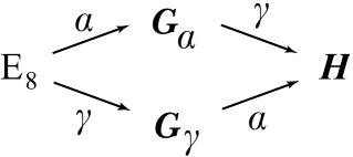
Figure 4: Entwined branching pattern induced by multiple lattice projections at a brane intersection.

In what follows we will refer to an entwined branching pattern such as the one shown in Figure 4 using the notation $(\,{\cal G}_{\alpha}\,,\,{\cal G}_{\gamma}\,|\,{\cal H}\,)$.

As described above, there are twelve complementary pairs of $\alpha\beta\gamma$-invariant four-planes: twelve such planes inside the ten-plane at the upper end-of-the-world are paired with twelve more inside the lower end-of-the-world. Elements of a pair are linked by interpolating $\alpha\gamma$-invariant five-planes. Furthermore each $\alpha\beta$-invariant six-plane and each $\beta\gamma$-invariant six-plane is a source of $G$-flux. In our usual terminology, we say that these planes have associated magnetic charges. These are the M-theory analogs of RR charges in string theory. Owing to global considerations, which can be derived by integrating the closed form $dG$ over five-cycles in the compact space, one deduces that the sum of these charges must vanish. This is the M-theory analog of the requirement of tadpole infinity cancellation in string theory. As explained in [14] this imposes that $\alpha$ and $\gamma$ must act on the two $E_{8}$ lattices in a complementary fashion. Thus, if we have a $(\,{\cal G}_{\alpha}\,,\,{\cal G}_{\gamma}\,|\,{\cal H})$ breakdown choice on the upper ten-plane, we must choose a fully complementary choice ( ${\cal G}_{\alpha}^{\prime}\,,\,{\cal G}_{\gamma}^{\prime}\,|\,{\cal H}^{\prime}\,)$ on the lower ten-plane. Complimentary in this case means that ${\cal G}_{\alpha}$ and ${\cal G}_{\alpha}^{\prime}$ must be chosen one-each from the pair of subgroups $E_{7}\times SU_{2}$ and $SO_{16}$ and, similarly, ${\cal G}_{\gamma}$ and ${\cal G}_{\gamma}^{\prime}$ must be chosen one-each from the pair of subgroups $E_{6}\times SU_{3}$ and $SU_{9}$. The groups ${\cal H}$ and ${\cal H}^{\prime}$ then depend on the choices made. Owing to this requirement, the number of global possibilities is severely limited. Requiring that any additional four dimensional gauge or mixed anomalies can be eliminated restricts the choices even further.

Now, keeping all of these considerations in mind, we proceed to study the situation at one of the $\alpha\beta\gamma$-invariant intersections, say one in the upper end-of-the-world. Once we find a consistently entwined branching which has curable four-dimensional intersection anomalies, we are then faced with the additional requirement of finding a consistently entwined complementary branching, associated with an $\alpha\beta\gamma$-plane in the lower end-of-the-world, which also has curable four-dimensional intersection anomalies. Ostensibly, there are four possibilities for choosing intermediate groups $(\,{\cal G}_{\alpha}\,,\,{\cal G}_{\gamma}\,)$ from the allowed possibilities. These four possibilities consist of two complimentary pairs however. The first of these is the choice $(\,E_{7}\times SU_{2}\,,\,E_{6}\times SU_{3}\,)$ which is complimentary to $(\,SO_{16}\,,\,SU_{9}\,)$. The second is the choice $(\,E_{7}\times SU_{2}\,,\,SU_{9}\,)$ which is complimentary to $(\,SO_{16}\,,\,E_{6}\times SU_{3}\,)$. We have discerned a consistent picture free from four-dimensional anomalies only for the second of these two choices.

We proceed to explain completely the consistent solution to the constraints described above. First we describe the situation at one of the “upstairs vertices” (i.e. one of the $\alpha\beta\gamma$-invariant intersections within the upper end-of-the-world) and then we describe the complimentary situation at one of the “downstairs vertices” (i.e. one of the $\alpha\beta\gamma$-invariant intersections within the lower end-of-the-world). In each case we exhibit the entwined branching patterns and identify the entwined subgroups, ${\cal H}$ upstairs and ${\cal H}^{\prime}$ downstairs. We also describe the chiral spectrum which survives the projections to four-dimensions, and explicitly demonstrate the absence of four-dimensional anomalies.

3.1 Upstairs Vertices

The generators $\alpha$ and $\gamma$ act on the lattice associated with the upstairs $E_{8}$ gauge factor according to $(\,E_{7}\times SU_{2}\,,\,SU_{9}\,|\,SU_{6}\times SU_{3}\times U_{1}\,)$. We verify that the subgroup ${\cal H}=SU_{6}\times SU_{3}\times U_{1}$ is consistently entwined inside of $E_{8}$ by $E_{7}\times SU_{2}$ and $SU_{9}$ by using two important consistency checks. First, we verify that $E_{8}$ branches to precisely the same representation of ${\cal H}$ when the branching occurs via each of the two separate routes indicated in Figure 4. Then we verify that there are no non-curable four-dimensional anomalies localized at the intersection. When we refer to a “consistently entwined” branching we are indicating that both of these criteria are met.

First, we consider the $(\alpha,\gamma)$ branching, under which the $E_{8}$ lattice is projected first via $\alpha$ to ${\cal G}_{\alpha}$, and then this subgroup is projected, via $\gamma$, to ${\cal H}$. For the case at hand, we have

$$E_{8} \stackrel{{\scriptstyle\alpha}}{{\longrightarrow}} E_{7}\times SU_{2}$$

$$\stackrel{{\scriptstyle\gamma}}{{\longrightarrow}} SU_{6}\times SU_{3}\times U_{1}$$

$${\bf 248} \stackrel{{\scriptstyle\alpha}}{{\longrightarrow}} [\,(\,{\bf 133}\,,\,{\bf 1}\,)\,\oplus\,(\,{\bf 1}\,,\,{\bf 3}\,)\,]\,\oplus\,(\,{\bf 56}\,,\,{\bf 2}\,)$$ (2)

$$\stackrel{{\scriptstyle\gamma}}{{\longrightarrow}} [\,(\,{\bf 35}\,,\,{\bf 1}\,)_{0}\,\oplus\,(\,{\bf 1}\,,\,{\bf 8}\,)_{0}\,\oplus\,(\,{\bf 15}\,,\,{\bf\bar{3}}\,)_{0}\,\oplus\,(\,{\bf\bar{15}}\,,\,{\bf 3}\,)_{0}$$

$$\oplus\,(\,{\bf 1}\,,\,{\bf 1}\,)_{+6}\,\oplus\,(\,{\bf 1}\,,\,{\bf 1}\,)_{0}\,\oplus\,(\,{\bf 1}\,,\,{\bf 1}\,)_{-6}\,]$$

$$\oplus\,(\,{\bf 20}\,,\,{\bf 1}\,)_{+3}\,\oplus\,(\,{\bf 6}\,,\,{\bf 3}\,)_{+3}\,\oplus\,(\,{\bf\bar{6}}\,,\,{\bf\bar{3}}\,)_{+3}$$

$$\oplus\,(\,{\bf 20}\,,\,{\bf 1}\,)_{-3}\,\oplus\,(\,{\bf\bar{6}}\,,\,{\bf\bar{3}}\,)_{-3}\,\oplus\,(\,{\bf 6}\,,\,{\bf 3}\,)_{-3}\,.$$

where we have chosen a convenient normalization for the $U(1)$ charge. As a useful mnemonic, we have placed brackets around those terms in the representation sum which correspond to the adjoint of ${\cal G}_{\alpha}$. This is useful for determining how the element $\alpha$ acts on the $E_{8}$ lattice. Since $\alpha$ breaks $E_{8}$ down to ${\cal G}_{\alpha}$, it follows that $\alpha$ acts trivially on those root vectors corresponding to the bracketed representations, and acts non-trivially on the representations which are not bracketed..

Next, we consider the $(\gamma,\alpha)$ branching, under which the $E_{8}$ lattice is projected first via $\gamma$ to ${\cal G}_{\gamma}$, and then this subgroup is projected via $\alpha$ to ${\cal H}$. For the case at hand, we have

$$E_{8} \stackrel{{\scriptstyle\gamma}}{{\longrightarrow}} SU_{9}$$

$$\stackrel{{\scriptstyle\alpha}}{{\longrightarrow}} SU_{6}\times SU_{3}\times U_{1}$$

$${\bf 248} \stackrel{{\scriptstyle\gamma}}{{\longrightarrow}} [\,{\bf 80}\,]\,\oplus\,{\bf 84}\,\oplus\,{\bf\bar{84}}$$ (3)

$$\stackrel{{\scriptstyle\alpha}}{{\longrightarrow}} [\,(\,{\bf 35}\,,\,{\bf 1}\,)_{0}\,\oplus\,(\,{\bf 1}\,,\,{\bf 8}\,)_{0}\,\oplus\,(\,{\bf 1}\,,\,{\bf 1}\,)_{0}\,\oplus\,(\,{\bf 6}\,,\,{\bf 3}\,)_{+3}\,\oplus\,(\,{\bf\bar{6}}\,,\,{\bf\bar{3}}\,)_{-3}\,]$$

$$\oplus\,(\,{\bf 20}\,,\,{\bf 1}\,)_{+3}\,\oplus\,(\,{\bf 15}\,,\,{\bf\bar{3}}\,)_{0}\,\oplus\,(\,{\bf 6}\,,\,{\bf 3}\,)_{-3}\,\oplus\,(\,{\bf 1}\,,\,{\bf 1}\,)_{-6}$$

$$\oplus\,(\,{\bf 20}\,,\,{\bf 1}\,)_{-3}\,\oplus\,(\,{\bf\bar{15}}\,,\,{\bf 3}\,)_{0}\,\oplus\,(\,{\bf\bar{6}}\,,\,{\bf\bar{3}}\,)_{+3}\,\oplus\,(\,{\bf 1}\,,\,{\bf 1}\,)_{+6}$$

We have enclosed with brackets those terms in the representation sum corresponding to the adjoint of ${\cal G}_{\gamma}$. Not surprisingly, these are not the same terms enclosed by the brackets in (2). Since $\gamma$ breaks $E_{8}$ down to ${\cal G}_{\gamma}$, it follows that $\gamma$ acts trivially on those $E_{8}$ root vectors corresponding to the bracketed representations, and non-trivially otherwise. We notice that the ultimate representations in (2) and (3) are the same. Thus, ${\cal H}=SU_{6}\times SU_{3}\times U_{1}$ satisfies the first necessary condition for the indicated branchings to be consistently entwined. We will analyze the second necessary condition, the absence of non-curable four-dimensional anomalies, shortly.

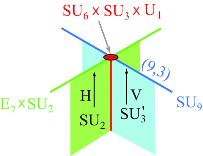
Figure 5: The neighborhood of one of the $\alpha\beta\gamma$-invariant four-plane intersections inside the upper end-of-the-world. Indicated in this diagram are the $E_{8}$ subgroups ${\cal G}_{\alpha}=E_{7}\times SU_{2}$ and ${\cal G}_{\gamma}=SU_{9}$ which survive on the $\alpha\beta$-invariant six-plane (the green line) and the $\beta\gamma$-invariant six-plane (the blue line), respectively. Also indicated is the representation of the six-dimensional twisted hypermultiplet needed to cure six-dimensional anomalies locally on the $\beta\gamma$-plane.

In generic situations, one way to analyze the problem of finding entwined branchings is to scan the lists of subgroups, depth by depth by referring to the tables in [23] or [24], and look for ostensible matches. One then has to carefully evaluate the branching rules in order to see if the selected higher-depth common group is, in fact properly entwined. One illustrative example is the following. If we were seeking an entwined branching which involved as intermediaries the $E_{8}$ subgroups $(\,SO_{16}\,,\,SU_{9}\,)$, we would discover that each of these group have $SU_{8}\times U_{1}$ subgroups. Thus, we would consider the possibility $(\,SO_{16}\,,\,SU_{9}\,|\,SU_{8}\times U_{1}\,)$. In this case, however, the ultimate representations do not coincide, as can be verified by direct computation. We conclude, therefore, that the group $SU_{8}\times U_{1}$ cannot be properly entwined inside of $E_{8}$ by the subgroups $SO_{16}$ and $SU_{9}$.

Two convenient ways of exhibiting some of the relevant branching information described by (2) and (3) is to use branching diagrams or branching tables, two tools which were introduced in [14]. For the case at hand, the relevant branching diagram and branching table are shown in Table 3.

248	$\alpha$	$\beta$	$\gamma$
$(\,{\bf 35}\,,\,{\bf 1}\,)_{0}$	+	+	+
$(\,{\bf 1}\,,\,{\bf 8}\,)_{0}$	+	+	+
$(\,{\bf 1}\,,\,{\bf 1}\,)_{0}$	$+$	+	+
$(\,{\bf 1}\,,\,{\bf 1}\,)_{-6}\,\oplus(\,{\bf 1}\,,\,{\bf 1}\,)_{+6}$	$+$	+	1/3
$(\,{\bf 15}\,,\,{\bf\bar{3}}\,)_{0}\,\oplus(\,{\bf\bar{15}}\,,\,{\bf 3}\,)_{0}$	+	+	1/3
$(\,{\bf 20}\,,\,{\bf 1}\,)_{+3}\,\oplus(\,{\bf 20}\,,\,{\bf 1}\,)_{-3}$	$-$	+	1/3
$(\,{\bf 6}\,,\,{\bf 3}\,)_{-3}\,\oplus(\,{\bf\bar{6}}\,,\,{\bf\bar{3}}\,)_{+3}$	$-$	+	1/3
$(\,{\bf 6}\,,\,{\bf 3}\,)_{+3}\,\oplus(\,{\bf\bar{6}}\,,\,{\bf\bar{3}}\,)_{-3}$	$-$	+	+
$E_{8}\to SU_{6}\times SU_{3}\times U_{1}$	$E_{7}\times SU_{2}$	$E_{8}$	$SU_{9}$

Table 3: Embedding diagram and branching table describing $E_{8}\to SU_{6}\times SU_{3}\times U_{1}$.

The branching diagram is a simplified “map” of the group $E_{8}$, showing, by dimensionality of subspaces, how the various subgroups are embedded. The numbers in this diagram each refer to the dimensionality of one of the representations of ${\cal H}$ included in the representation sums in (2) or, equivalently, (3). The branching table indicates the action of the generating elements $\alpha$, $\beta$ and $\gamma$ on the $E_{8}$ root lattice, by showing how these elements act on the representation indices associated with fields taking values in those representations of ${\cal H}$.

From the information included in the branching table and the embedding diagram, it is straightforward to determine the spectrum which arises from the ten-dimensional $E_{8}$ fields which survive projection at the four-dimensional intersection. This is done by decomposing the ten-dimensional vector fields into four dimensional vector and scalar fields, and then considering the combination of the tensorial action induced by the quotient group elements, via their action on the spacetime coordinates, with the additional action on the representation indices associated with these same fields as induced by the action of the quotient group on the $E_{8}$ lattice. The upshot, for the ten-dimensional fields, is that representations in the branching table transforming under $(\alpha,\beta,\gamma)$ as $(+,+,+)$ supply $N=1$ vector multiplets. In the next case, representations transforming as $(-,+,+)$ supply $N=1$ chiral multiplets transforming according to the indicated representation. The remaining cases, $(+,+,\pm 1/3)$ and $(-,+,\mp 1/3)$ correspond to complex representations of the sort ${\bf{\cal R}}\oplus{\bf\bar{\cal R}}$. These also supply chiral multiplets, but the representation is truncated to ${\bf{\cal R}}$ or to ${\bf\bar{\cal R}}$, depending on the respective sign on the $1/3$ which appears in the branching table.

It is now straightforward to read off of the branching table in Figure 3 the contribution to the four dimensional intersection spectrum which arises from the $E_{8}$ fields. For the case at hand, using the rules described in the previous paragraph, we determine the spectrum indicated in the first column of Table 4. The rational prefactors which appear in that table are distribution coefficients which we need to include in the computation of the four-dimensional anomaly. These are described below. Notice that there are other contributions to the four-dimensional spectrum apparent in Figure 4. Notably, we have six-dimensional twisted fields which need to be considered. We describe these fields presently.

As described above, in order to cancel the six-dimensional anomaly on the $\beta\gamma$-invariant six-planes, we must include $SU_{3}^{\prime}$ Yang-Mills supermultiplets on the intersecting $\gamma$-invariant seven-plane. We must also include six-dimensional “twisted” hypermultiplets on the $\beta\gamma$-planes themselves, transforming as $(\,{\bf 9}\,,\,{\bf 3}\,)$ under $SU_{9}\times SU_{3}^{\prime}$. These reduce at the four-dimensional intersection into one $N=1$ chiral and one $N=1$ anti-chiral multiplet transforming as determined by the following branching,

$$SU_{9}\times SU_{3}^{\prime} \longrightarrow SU_{6}\times SU_{3}\times SU_{3}^{\prime}\times U_{1}$$

$$(\,{\bf 9}\,,\,{\bf 3}\,) \longrightarrow (\,{\bf 6}\,,\,{\bf 1}\,,\,{\bf 3}\,)_{-1}\,\oplus\,(\,{\bf 1}\,,\,{\bf 3}\,,\,{\bf 3}\,)_{+2}\,.$$ (4)

On the $\alpha\beta\gamma$-invariant four-planes, however, the $\mathbb{Z}_{2}$ generator $\alpha$ projects this to one chiral multiplet (i.e. we project out the anti-chiral multiplet). This explains the fields which appear in the “6D” column in Figure 4. The collective situation at one of the upstairs four-planes is illustrated in Figure 5. In that figure we can see the variety of fixed-planes which mutually intersect at the given four-plane. We can also see the effective gauge group and the spectrum of twisted fields associated with the each of these planes.

	10D	7D	6D	4D
Chiral	${\textstyle\frac{1}{12}}\,(\,{\bf 1}\,,\,{\bf 1}\,,\,{\bf 1}\,)_{-6}$	${\textstyle\frac{1}{6}}\,(\,{\bf 1}\,,\,{\bf 1}\,,\,{\bf 1}\,)_{0}$	${\textstyle\frac{1}{4}}\,(\,{\bf 6}\,,\,{\bf 1}\,,\,{\bf 3}\,)_{-1}$
	${\textstyle\frac{1}{12}}\,(\,{\bf 15}\,,\,{\bf\bar{3}}\,,\,{\bf 1}\,)_{0}$	${\textstyle\frac{1}{6}}\,(\,{\bf 1}\,,\,{\bf 1}\,,\,{\bf 1}\,)_{+3}$	${\textstyle\frac{1}{4}}\,(\,{\bf 1}\,,\,{\bf 3}\,,\,{\bf 3}\,)_{+2}$
	${\textstyle\frac{1}{12}}\,(\,{\bf 20}\,,\,{\bf 1}\,,\,{\bf 1}\,)_{+3}$	${\textstyle\frac{1}{6}}\,(\,{\bf 1}\,,\,{\bf 1}\,,\,{\bf 1}\,)_{-3}$
	${\textstyle\frac{1}{12}}\,(\,{\bf 6}\,,\,{\bf 3}\,,\,{\bf 1}\,)_{-3}$
	${\textstyle\frac{1}{12}}\,(\,{\bf 6}\,,\,{\bf 3}\,,\,{\bf 1}\,)_{+3}$
	${\textstyle\frac{1}{12}}\,(\,{\bf\bar{6}}\,,\,{\bf\bar{3}}\,,\,{\bf 1}\,)_{-3}$
Vector	${\textstyle\frac{1}{12}}\,(\,{\bf 35}\,,\,{\bf 1}\,,\,{\bf 1}\,)_{0}$	${\textstyle\frac{1}{8}}\,(\,{\bf 1}\,,\,{\bf 1}\,,\,{\bf 8}\,)_{0}$
	${\textstyle\frac{1}{12}}\,(\,{\bf 1}\,,\,{\bf 8}\,,\,{\bf 1}\,)_{0}$
	${\textstyle\frac{1}{12}}\,(\,{\bf 1}\,,\,{\bf 1}\,,\,{\bf 1}\,)_{0}$

Table 4: The effective spectrum, in terms of $N=1$ superfields, as seen by one of the upstairs $\alpha\beta\gamma$ four-planes, in terms of representations of $SU_{6}\times SU_{3}\times SU_{3}^{\prime}\times U_{1}$. The rational numbers which appear in this table are the distribution coefficients needed to amend the index theory computation of the local four-dimensional anomalies.

The seven-dimensional twisted fields, localized on the $\alpha$-invariant and $\gamma$-invariant seven-planes also contribute effectively to the local four-dimensional spectrum. However, these fields do not contribute chirally, and are not relevant to the four-dimensional anomaly discussion.

A four dimensional anomaly arises because the higher-dimensional fermion fields couple in a chiral fashion locally, at the four-dimensional intersection, to the gauge currents associated with ${\cal H}$. As is well-known, the index-theory computation of the relevant anomalies needs to be modified by the incorporation of appropriate distribution divisors. For instance, since a given $\beta\gamma$-invariant six-plane plane shares four $\alpha\beta\gamma$-invariant four-planes as subspaces, the four-dimensional anomaly associated with a given $\beta\gamma$ plane includes a distribution divisor of 4. Similarly, the ten-dimensional contribution to the four-dimensional anomaly should include a distribution divisor of twelve. This is obtained from the observation that each $\beta$-invariant ten-plane includes twelve indistinguishable $\alpha\beta\gamma$-invariant four planes, as is evident in Figure 2.

The charged chiral spectrum “seen” by a given $\alpha\beta\gamma$ four-plane, in terms of $SU_{6}\times SU_{3}\times SU_{3}^{\prime}\times U_{1}$ representations, consists of the following terms derived from ten dimensions,

$$\frac{1}{12}\,\Big{(}\,(\,{\bf 1}\,,\,{\bf 1}\,,\,{\bf 1}\,)_{-6}\,\oplus\,(\,{\bf 20}\,,\,{\bf 1}\,,\,{\bf 1}\,)_{+3}\,\oplus\,(\,{\bf 6}\,,\,{\bf 3}\,,\,{\bf 1}\,)_{-3}\,\Big{)}$$ (5)

and also the following terms derived from six dimensions,

$$\frac{1}{4}\,\Big{(}\,(\,{\bf 6}\,,\,{\bf 1}\,,\,{\bf 3}\,)_{-1}\,\oplus\,(\,{\bf 1}\,,\,{\bf 3}\,,\,{\bf 3}\,)_{+2}\,\Big{)}\,.$$ (6)

In each case, the rational pre-factor is the anomaly distribution coefficient. Using the chiral spectrum shown in (5) and (6), we can now compute the the four-dimensional gauge anomaly seen by one of the $\alpha\beta\gamma$ planes. The precise technology for doing this is explained in Appendix A. The relevant anomalies are the gauge anomalies for the simple factors $SU_{6}$, $SU_{3}$ and $SU_{3}^{\prime}$, the gauge anomaly for the $U_{1}$ factor, and the mixed anonaly involving the $U_{1}$ factor. These can be computed using (15) and (16). We find,

$$I(\,SU_{6}\,) = {\textstyle\frac{1}{12}}\,\Big{(}\,1\,(+3)\,I_{2}({\bf 20})+3\,(-3)\,I_{2}({\bf 6})\,\Big{)}+{\textstyle\frac{1}{4}}\,\Big{(}\,3(-1)\,I_{2}({\bf 6})\,\Big{)}$$

$$I(\,SU_{3}\,) = {\textstyle\frac{1}{12}}\,\Big{(}\,6\,(-3)\,I_{2}(\,{\bf 3}\,)\,\Big{)}+{\textstyle\frac{1}{4}}\,\Big{(}\,3\,(+2)\,I_{2}(\,{\bf 3}\,)\,\Big{)}$$

$$I(\,SU_{3}^{\prime}\,) = {\textstyle\frac{1}{4}}\,\Big{(}\,6\,(-1)+3\,(+2)\,\Big{)}\,I_{2}(\,{\bf 3}\,)$$

$$I(\,U_{1}\,)_{\rm GAUGE} = {\textstyle\frac{1}{12}}\,\Big{(}\,1\,(-6)^{3}+20\,(+3)^{3}+18\,(-3)^{3}\,\Big{)}+{\textstyle\frac{1}{4}}\,\Big{(}\,18\,(-1)^{3}+9\,(+2)^{3}\,\Big{)}$$

$$I(U_{1})_{\rm MIXED} = {\textstyle\frac{1}{12}}\,\Big{(}\,1\,(-6)+20\,(+3)+18\,(-3)\,\Big{)}+{\textstyle\frac{1}{4}}\,\Big{(}\,18\,(-1)+9\,(+2)\,\Big{)}\,,$$ (7)

where $I_{2}({\bf{\cal R}})$ denotes the second index associated with the representation ${\bf{\cal R}}$. For $SU({\bf N})$, the second index of the fundamental ${\bf N}$ representations are always unity, i.e. $I_{2}({\bf N})=1$. Thus, for $SU_{6}$, we have $I_{2}(\,{\bf 6}\,)=1$, and for each of the two $SU(3)$ factors we have $I_{2}(\,{\bf 3}\,)=1$. The ${\bf 20}$ is the three-index antisymmetric tensor representation of $SU_{6}$. Therefore, we use the algorithm explained in Appendix B to compute $I_{2}(\,{\bf 20}\,)=6$. Using these results, it is easy to show that each of the five anomaly expressions in (7) vanishes identically. Thus, we have satisfied the second non-trivial check that the entwined branching $(\,E_{7}\times SU_{2}\,,\,SU_{9}\,|\,SU_{6}\times SU_{3}\times U_{1}\,)$ is, in fact consistent.

3.2 Downstairs Vertices

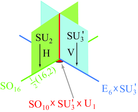
Figure 6: The neighborhood of one of the $\alpha\beta\gamma$-invariant four-plane intersections inside the lower end-of-the-world. Indicated in this diagram are the $E_{8}$ subgroups ${\cal G}_{\alpha}=SO_{16}$ and ${\cal G}_{\gamma}=E_{6}\times SU_{3}$ which survive on the $\alpha\beta$-invariant six-plane (the green line) and the $\beta\gamma$-invariant six-plane (the blue line), respectively. Also indicated is the representation of the six-dimensional twisted hypermultiplet needed to cure six-dimensional anomalies locally on the $\beta\gamma$-plane.

Owing to global $G$-flux conservation, we are obligated to incorporate on the downstairs vertices consistently entwined branchings complimentary to that discussed above. We have determined that the following is satisfactory $(\,SO_{16}\,,\,E_{6}\times SU_{3}^{\prime}\,|\,SO_{10}\times SU_{3}^{\prime}\times U_{1}^{\prime}\,)$. We suspect this is the unique solution. In this subsection we will analyze the branching and anomaly questions pertaining to this choice in a manner analogous to the discussion in the previous subsection. Since the reasoning is identical, we will be comparatively brief. For the case at hand, the $(\,\alpha\,,\,\gamma\,)$ branching is given by

$$E_{8} \stackrel{{\scriptstyle\alpha}}{{\longrightarrow}} SO_{16}$$

$$\stackrel{{\scriptstyle\gamma}}{{\longrightarrow}} SO_{10}\times SU_{3}^{\prime}\times U_{1}^{\prime}$$

$${\bf 248} \stackrel{{\scriptstyle\alpha}}{{\longrightarrow}} [\,{\bf 120}\,]\,\oplus\,{\bf 128}$$ (8)

$$\stackrel{{\scriptstyle\gamma}}{{\longrightarrow}} [\,(\,{\bf 45}\,,\,{\bf 1}\,)_{0}\,\oplus\,(\,{\bf 1}\,,\,{\bf 8}\,)_{0}\,\oplus\,(\,{\bf 1}\,,\,{\bf 1}\,)_{0}$$

$$\oplus\,(\,{\bf 10}\,,\,{\bf 3}\,)_{-2}\,\oplus\,(\,{\bf 10}\,,\,{\bf\bar{3}}\,)_{+2}\,\oplus\,(\,{\bf 1}\,,\,{\bf 3}\,)_{+4}\,\oplus\,(\,{\bf 1}\,,\,{\bf\bar{3}}\,)_{-4}\,]$$

$$\,\oplus\,(\,{\bf 16}\,,\,{\bf 1}\,)_{-3}\,\oplus\,(\,{\bf 16}\,,\,{\bf 3}\,)_{+1}\,\oplus\,(\,{\bf\bar{16}}\,,\,{\bf 1}\,)_{+3}\,\oplus\,(\,{\bf\bar{16}}\,,\,{\bf\bar{3}}\,)_{-1}\,.$$

Next, for the $(\gamma,\alpha)$ branching, we find

$$E_{8} \stackrel{{\scriptstyle\gamma}}{{\longrightarrow}} E_{6}\times SU_{3}^{\prime}$$

$$\stackrel{{\scriptstyle\alpha}}{{\longrightarrow}} SO_{10}\times SU_{3}^{\prime}\times U_{1}^{\prime}$$

$${\bf 248} \stackrel{{\scriptstyle\gamma}}{{\longrightarrow}} [\,(\,{\bf 78}\,,\,{\bf 1}\,)\,\oplus\,(\,{\bf 1}\,,\,{\bf 8}\,)\,]\,\oplus\,(\,{\bf 27}\,,\,{\bf 3}\,)\,\oplus\,(\,{\bf\bar{27}}\,,\,{\bf\bar{3}}\,)$$ (9)

$$\stackrel{{\scriptstyle\alpha}}{{\longrightarrow}} [\,(\,{\bf 45}\,,\,{\bf 1}\,)_{0}\,\oplus\,(\,{\bf 16}\,,\,{\bf 1}\,)_{-3}\,\oplus\,(\,{\bf\bar{16}}\,,\,{\bf 1}\,)_{+3}\,\oplus\,(\,{\bf 1}\,,\,{\bf 1}\,)_{0}\,\oplus\,(\,{\bf 1}\,,\,{\bf 8}\,)_{0}\,]$$

$$\oplus\,(\,{\bf 16}\,,\,{\bf 3}\,)_{+1}\,\oplus\,(\,{\bf 10}\,,\,{\bf 3}\,)_{-2}\,\oplus\,(\,{\bf 1}\,,\,{\bf 3}\,)_{+4}$$

$$\oplus\,(\,{\bf\bar{16}}\,,\,{\bf\bar{3}}\,)_{-1}\,\oplus\,(\,{\bf 10}\,,\,{\bf\bar{3}}\,)_{+2}\,\oplus\,(\,{\bf 1}\,,\,{\bf\bar{3}}\,)_{-4}$$

Once again, notice that the ultimate representations in (8) and (9) coincide. As described above, this is a necessary condition on entwined branchings. Relevant aspects of this branching are usefully exhibited in the embedding diagram and branching table shown in Figure 5.

248	$\alpha$	$\beta$	$\gamma$
$(\,{\bf 45}\,,\,{\bf 1}\,)_{0}$	+	+	+
$(\,{\bf 1}\,,\,{\bf 8}\,)_{0}$	+	+	+
$(\,{\bf 1}\,,\,{\bf 1}\,)_{0}$	+	+	+
$(\,{\bf 10}\,,\,{\bf 3}\,)_{-2}\,\oplus\,(\,{\bf\bar{10}}\,,\,{\bf\bar{3}}\,)_{+2}$	+	+	1/3
$(\,{\bf 1}\,,\,{\bf 3}\,)_{+4}\,\oplus\,(\,{\bf\bar{1}}\,,\,{\bf\bar{3}}\,)_{-4}$	+	+	1/3
$(\,{\bf 16}\,,\,{\bf 1}\,)_{-3}\,\oplus\,(\,{\bf\bar{16}}\,,\,{\bf 1}\,)_{+3}$	$-$	+	+
$(\,{\bf 16}\,,\,{\bf 3}\,)_{+1}\,\oplus\,(\,{\bf\bar{16}}\,,\,{\bf\bar{3}}\,)_{-1}$	$-$	+	1/3
$E_{8}\to SO_{10}\times SU_{3}^{\prime}\times U_{1}$	$SO_{16}$	$E_{8}$	$E_{6}\times SU_{3}^{\prime}$

Table 5: Embedding diagram and branching table describing $E_{8}\to SO_{10}\times SU_{3}^{\prime}\times U_{1}$.

In order to cancel local anomalies on the $\alpha\gamma$-invariant six-planes, we must include $SU_{2}$ Yang-Mills supermultiplets on the intersecting $\alpha$-invariant seven-plane. We must also include twisted hypermultiplets on the $\alpha\gamma$-planes themselves, transforming as ${\textstyle\frac{1}{2}}(\,{\bf 16}\,,\,{\bf 2}\,)$ under $SO_{16}\times SU_{2}$. These reduce at the four-dimensional intersection into one $N=1$ chiral multiplet transforming under $SO_{10}\times SU_{3}^{\prime}\times U_{1}^{\prime}$ as determined by the following branching,

$$SO_{16}\times SU_{2} \longrightarrow SO_{10}\times SU_{4}\times SU_{2}$$

$$\longrightarrow SO_{10}\times SU_{3}^{\prime}\times SU_{2}\times U_{1}^{\prime}$$

$$(\,{\bf 16}\,,\,{\bf 2}\,) \longrightarrow (\,{\bf 10}\,,\,{\bf 1}\,,\,{\bf 2}\,)\,\oplus\,(\,{\bf 1}\,,\,{\bf 6}\,,\,{\bf 2}\,)$$ (10)

$$\longrightarrow (\,{\bf 10}\,,\,{\bf 1}\,,\,{\bf 2}\,)_{0}\,\oplus\,(\,{\bf 1}\,,\,{\bf 3}\,,\,{\bf 2}\,)_{+2}\,\oplus\,(\,{\bf 1}\,,\,{\bf\bar{3}}\,,\,{\bf 2}\,)_{-2}$$

On the $\alpha\beta\gamma$-invariant four-planes, the $\mathbb{Z}_{3}$ generator $\gamma$ acts trivially on these six-dimensional twisted fields and, does not serve to reduce further the degrees of freedom. Since a given $\alpha\beta$-invariant six-plane shares three $\alpha\beta\gamma$-invariant four-planes as subspaces, the four-dimensional anomaly associated with fields on a given $\beta\gamma$-invariant six-plane includes a distribution divisor of three. Therefore, these fields contribute to the effective four-dimensional spectrum those fields indicated in the “6D” column of Table 6. The collective situation at one of the downstairs four-planes is illustrated in Figure 6.

	10D	7D	6D	4D
Chiral	${\textstyle\frac{1}{12}}\,(\,{\bf 10}\,,\,{\bf 3}\,,\,{\bf 1}\,)_{-2}$	${\textstyle\frac{1}{8}}\,(\,{\bf 1}\,,\,{\bf 8}\,,\,{\bf 1}\,)_{0}$	${\textstyle\frac{1}{3}}\,(\,{\bf 10}\,,\,{\bf 1}\,,\,{\bf 2}\,)_{0}$
	${\textstyle\frac{1}{12}}\,(\,{\bf 1}\,,\,{\bf 3}\,,\,{\bf 1}\,)_{+4}$		${\textstyle\frac{1}{3}}\,(\,{\bf 1}\,,\,{\bf 3}\,,\,{\bf 2}\,)_{+2}$
	${\textstyle\frac{1}{12}}\,(\,{\bf 16}\,,\,{\bf 3}\,,\,{\bf 1}\,)_{+1}$		${\textstyle\frac{1}{3}}\,(\,{\bf 1}\,,\,{\bf\bar{3}}\,,\,{\bf 2}\,)_{-2}$
	${\textstyle\frac{1}{12}}\,(\,{\bf 16}\,,\,{\bf 1}\,,\,{\bf 1}\,)_{-3}$
	${\textstyle\frac{1}{12}}\,(\,{\bf\bar{16}}\,,\,{\bf 1}\,,\,{\bf 1}\,)_{+3}$
Vector	${\textstyle\frac{1}{12}}\,(\,{\bf 45}\,,\,{\bf 1}\,,\,{\bf 1}\,)_{0}$	${\textstyle\frac{1}{6}}\,(\,{\bf 1}\,,\,{\bf 1}\,,\,{\bf 3}\,)_{0}$
	${\textstyle\frac{1}{12}}\,(\,{\bf 1}\,,\,{\bf 8}\,,\,{\bf 1}\,)_{0}$
	${\textstyle\frac{1}{12}}\,(\,{\bf 1}\,,\,{\bf 1}\,,\,{\bf 1}\,)_{0}$

Table 6: The effective spectrum, in terms of $N=1$ superfields, as seen by one of the downstairs $\alpha\beta\gamma$ four-planes, in terms of representations of $SO_{10}\times SU_{3}^{\prime}\times SU_{2}\times U_{1}^{\prime}$.

The charged chiral spectrum seen by a given $\alpha\beta\gamma$-invariant four-plane consists of the following terms derived from ten dimensions,

$$\frac{1}{12}\,\Big{(}\,(\,{\bf 10}\,,\,{\bf 3}\,,\,{\bf 1}\,)_{-2}\,\oplus\,(\,{\bf 1}\,,\,{\bf 3}\,,\,{\bf 1}\,)_{+4}\,\oplus\,(\,{\bf 16}\,,\,{\bf 3}\,,\,{\bf 1}\,)_{+1}\,\Big{)}\,.$$ (11)

The terms derived from six dimensions have no anomaly. In (11) the pre-factor one-twelfth is the anomaly distribution coefficient. As described above, this derives from the fact that there are twelve indistinguishable $\alpha\beta\gamma$-invariant four-planes within each $\beta$-invariant ten-plane. Using the chiral spectrum shown in (11), we can now compute the the four-dimensional gauge anomaly seen by one of the $\alpha\beta\gamma$ planes. This is done according to the rules explained in Appendix A. The relevant anomalies are the gauge anomalies for the simple factors $SO_{10}$ and $SU_{3}^{\prime}$, the gauge anomaly for the $U_{1}^{\prime}$ factor and the mixed anomaly involving the $U_{1}^{\prime}$ factor.

$$I(\,SO_{10}\,) = {\textstyle\frac{1}{12}}\,\Big{(}\,3\,(-2)\,I_{2}({\bf 10})+3\,(+1)\,I_{2}({\bf 16})\,\Big{)}$$

$$I(\,SU_{3}^{\prime}\,) = {\textstyle\frac{1}{12}}\,\Big{(}\,10\,(-2)+1\,(+4)+16\,(+1)\,\Big{)}\,I_{2}(\,{\bf 3}\,)$$

$$I(\,U_{1}\,)_{\rm GAUGE} = {\textstyle\frac{1}{12}}\,\Big{(}\,30\,(-2)^{3}+3\,(+4)^{3}+48\,(+1)^{3}\,\Big{)}$$

$$I(\,U_{1}\,)_{\rm MIXED} = {\textstyle\frac{1}{12}}\,\Big{(}\,30\,(-2)+3\,(+4)+48\,(+1)\,\Big{)}\,.$$ (12)

The second indices for the fundamental representations 10 of $SO(10)$ and ${\bf 3}$ of $SU(3)$ are unity by definition. Thus, $I_{2}({\bf 10})=1$ and $I_{2}({\bf 3})=1$ in (12). For integer $l$, the groups $SO(2l)$ have elementary spinor representations with dimension $2^{l-1}$. These representations have second index $2^{l-4}$. Thus, for $SO_{10}$, we have $I_{2}({\bf 16})=2$. Using these results, we easily show that each of the four anomaly expressions in (7) vanishes identically. Thus, we have satisfied the non-trivial check that the entwined branching $(\,SO_{16}\,,\,E_{6}\times SU_{3}^{\prime}\,|\,SO_{10}\times SU_{3}^{\prime}\times U_{1}^{\prime}\,)$ is, in fact, consistent.

At this point we have verified that all local anomalies in this orbifold, including those concentrated on ten-dimensional fixed planes, six-dimensional fixed planes and also four-dimensional fixed planes have been eliminated. The four-dimensional anomalies have been analyzed at the 24 $\alpha\beta\gamma$-invariant fixed planes, twelve on the upper end-of-the-world, and twelve on the lower end-of-the-world. One might wonder about possible four-dimensional anomalies localized at the other two classes of four-dimensional intersections which occur in this orbifold. One of these classes comprises the sixteen triple intersections of the $\alpha\gamma$-invariant six-planes (the grey spots in Figure 2). The other class comprises the twelve double intersections of the $\beta\gamma$-invariant six-planes (the yellow spots in Figure 2). In each of these cases the effective four-dimensional spectrum seen by these intersections is non-chiral. For this reason there are no four-dimensional anomaly constraints associated with these intersections. The fact that the effective spectrum at these points is non-chiral is related to the fact that these intersection points are not $\Gamma$-invariants, this in contrast to the $\alpha\beta\gamma$-invariant four-planes. (It is for a similar reason that the effective spectrum associated with the orbifold described in [14] is non-chiral.)

Notably, despite the chiral nature of the locally-observed spectrum, our solution does not require any extra four-dimensional twisted fields to remove the four-dimensional intersection anomalies. This was unexpected. In more general orbifolds we do expect that such four-dimensional local matter will be necessary. In fact, the circumstance in which the four-dimensional intersection anomalies would be non-trivially cured by the addition of new fields localized at intersections would be especially interesting.

4 When Worlds Collide

If we consider a limit where all compact dimensions except the interval direction $x^{11}$ are taken small, we obtain a picture of two four-dimensional ends-of-the-world, connected by a five-dimensional bulk. We shall refer to this as the “spindle” limit, since this describes a situation where the seven compact dimensions degenerate to a spindle shape. Chiral matter living on the the “upper world” (at the top of the spindle) transforms under $SU_{6}\times SU_{3}\times SU_{3}^{\prime}\times U_{1}$, whereas chiral matter living on the “lower world” (at the bottom of the spindle) transforms under $SO_{10}\times SU_{3}^{\prime}\times SU_{2}\times U_{1}^{\prime}$. The precise matter content corresponding to these two worlds is obtained from three different sources, corresponding to the three different classes of “neighborhoods” shown in Figure 3.

Primarily, there is the chiral spectrum associated with the $\alpha\beta\gamma$-invariant intersections analyzed in the previous section. The four-dimensional chiral spectrum obtained in the spindle limit is obtained for the upper world from Table 4 and for the lower world from Table 6. In the spindle limit, the contributions from the ten-dimensional twisted fields and from the six-dimensional twisted fields appear as chiral multiplets transforming according to representations indicated in those tables. However, as the compact space $X^{7}$ coalesces to a spindle, the associated anomaly distribution coefficients add up to unity. This, in fact, is what justified those coefficients in the first place. From the spindle point-of-view the seven-dimensional fields appearing in Tables 4 and 6 become five-dimensional (bulk) fields.

Next, there is the non-chiral spectrum associated with the the six-planes which do not have $\Gamma$-invariant subspaces. For instance, out of the nine $\beta\gamma$-invariant six-planes, three of these intersect $\alpha\beta$-invariant six-planes, and six do not. The associated six-dimensional twisted fields on the upper world are projected as in (4) in each case. However, in those three cases involving $\Gamma$-invariant intersections, the contribution to the four-dimensional spectrum consists exclusively of chiral multiplets transforming as indicated. (In those cases the antichiral components are projected out.) In the six remaining cases, where there are no $\Gamma$-invariant subspaces, the six-dimensional twisted fields provide complementary sets of chiral and anti-chiral multiplets, each transforming according to the representation on the right-hand side of (4). By charge-conjugation, however, this is equivalent to one set of chiral multiplets transforming in that same way, and another set of chiral multiplets transforming in the conjugate representation. Thus, the six $\beta\gamma$-invariant six-planes without $\Gamma$-invariant subspaces provide a non-chiral sector consisting of twelve sets of chiral multiplets, six of which transform under $SU_{6}\times SU_{3}\times SU_{3}^{\prime}\times U_{1}$ as ${\bf{\cal R}}\equiv(\,{\bf 6}\,,\,{\bf 1}\,,\,{\bf 3}\,)_{-1}\,\oplus\,(\,{\bf 1}\,,\,{\bf 3}\,,\,{\bf 3}\,)_{+2}$, and six more transforming as the conjugate of this representation. Adding these contributions together, we have nine sets of chiral fields transforming as ${\bf{\cal R}}$, and only six transforming as ${\bf\bar{{\cal R}}}$.

We also have six-dimensional twisted fields on the $\alpha\beta$-planes in the lower world. Each of the sixteen $\alpha\beta$-planes on the lower world supports fields transforming as shown in (10). In this case there is no further projection imparted at the $\Gamma$-invariant intersections. Therefore, the six-dimensional twisted fields in the lower world contributes to the four-dimensional spectrum sixteen indistinguishable non-chiral families.

Combining all of the above, we have determined two complimentary M-theory “worlds”. The respective four-dimensional chiral spectra, determined along the lines described above are summarized in Tables 8 and 8. These two worlds are connected by a five-dimensional “bulk”, which consists of minimal five-dimensional supergravity coupled to an $SU_{2}\times SU_{3}^{\prime}$ gauge sector.

$(\,{\bf 1}\,,\,{\bf 1}\,,\,{\bf 1}\,)_{-6}$	$9\,(\,{\bf 6}\,,\,{\bf 1}\,,\,{\bf 3}\,)_{-1}$
$(\,{\bf 15}\,,\,{\bf\bar{3}}\,,\,{\bf 1}\,)_{0}$	$6\,(\,{\bf\bar{6}}\,,\,{\bf 1}\,,\,{\bf\bar{3}}\,)_{+1}$
$(\,{\bf 20}\,,\,{\bf 1}\,,\,{\bf 1}\,)_{+3}$	$9\,(\,{\bf 1}\,,\,{\bf 3}\,,\,{\bf 3}\,)_{+2}$
$(\,{\bf 6}\,,\,{\bf 3}\,,\,{\bf 1}\,)_{-3}$	$6\,(\,{\bf 1}\,,\,{\bf\bar{3}}\,,\,{\bf\bar{3}}\,)_{-2}$
$(\,{\bf 6}\,,\,{\bf 3}\,,\,{\bf 1}\,)_{+3}$
$(\,{\bf\bar{6}}\,,\,{\bf\bar{3}}\,,\,{\bf 1}\,)_{-3}$

Table 7: The Upper World. Chiral multiplets transform as shown under $SU_{6}\times SU_{3}\times SU_{3}^{\prime}\times U_{1}$. Note that the $U_{1}$ factor here is a subgroup of the $SU_{2}$ factor which appears on the lower world. This is a chiral spectrum which is completely free of all gauge and mixed anomalies.

$(\,{\bf 10}\,,\,{\bf 3}\,,\,{\bf 1}\,)_{-2}$	$16\,(\,{\bf 10}\,,\,{\bf 1}\,,\,{\bf 2}\,)_{0}$
$(\,{\bf 1}\,,\,{\bf 3}\,,\,{\bf 1}\,)_{+4}$	$16\,(\,{\bf 1}\,,\,{\bf 3}\,,\,{\bf 2}\,)_{+2}$
$(\,{\bf 16}\,,\,{\bf 3}\,,\,{\bf 1}\,)_{+1}$	$16\,(\,{\bf 1}\,,\,{\bf\bar{3}}\,,\,{\bf 2}\,)_{-2}$
$(\,{\bf 16}\,,\,{\bf 1}\,,\,{\bf 1}\,)_{-3}$
$(\,{\bf\bar{16}}\,,\,{\bf 1}\,,\,{\bf 1}\,)_{+3}$

Table 8: The Lower World. Chiral multiplets transform as shown under $SO_{10}\times SU_{3}^{\prime}\times SU_{2}\times U_{1}^{\prime}$. This is a chiral spectrum which is completely free of all gauge and mixed anomalies.

If we now take another limit, whereby the one remaining compact dimension $x^{11}$ shrinks to zero size, then the upper and lower worlds coalesce. All fields then transform under $SO_{10}\times SU_{6}\times SU_{3}\times SU_{3}^{\prime}\times U_{1}\times U_{1}^{\prime}$, where $U_{1}\subset SU_{2}$. The chiral spectrum is then obtained by combining (8) and (8) by considering the relevant branching rules. For completeness, we include this spectrum in Table 9.

$(\,{\bf 1}\,,\,{\bf 1}\,,\,{\bf 1}\,,\,{\bf 1}\,)_{-6,0}$	$9\,(\,{\bf 1}\,,\,{\bf 6}\,,\,{\bf 1}\,,\,{\bf 3}\,)_{-1,0}$
$(\,{\bf 1}\,,\,{\bf 15}\,,\,{\bf\bar{3}}\,,\,{\bf 1}\,)_{0,0}$	$6\,(\,{\bf 1}\,,\,{\bf\bar{6}}\,,\,{\bf 1}\,,\,{\bf\bar{3}}\,)_{+1,0}$
$(\,{\bf 1}\,,\,{\bf 20}\,,\,{\bf 1}\,,\,{\bf 1}\,)_{+3,0}$	$9\,(\,{\bf 1}\,,\,{\bf 1}\,,\,{\bf 3}\,,\,{\bf 3}\,)_{+2,0}$
$(\,{\bf 1}\,,\,{\bf 6}\,,\,{\bf 3}\,,\,{\bf 1}\,)_{-3,0}$	$6\,(\,{\bf 1}\,,\,{\bf 1}\,,\,{\bf\bar{3}}\,,\,{\bf\bar{3}}\,)_{-2,0}$
$(\,{\bf 1}\,,\,{\bf 6}\,,\,{\bf 3}\,,\,{\bf 1}\,)_{+3,0}$
$(\,{\bf 1}\,,\,{\bf\bar{6}}\,,\,{\bf\bar{3}}\,,\,{\bf 1}\,)_{-3,0}$
$(\,{\bf 10}\,,\,{\bf 1}\,,\,{\bf 1}\,,\,{\bf 3}\,)_{0,-2}$	$16\,(\,{\bf 10}\,,\,{\bf 1}\,,\,{\bf 1}\,,\,{\bf 1}\,)_{+1,0}$
$(\,{\bf 1}\,,\,{\bf 1}\,,\,{\bf 1}\,,\,{\bf 3}\,)_{0,+4}$	$16\,(\,{\bf 10}\,,\,{\bf 1}\,,\,{\bf 1}\,,\,{\bf 1}\,)_{-1,0}$
$(\,{\bf 16}\,,\,{\bf 1}\,,\,{\bf 1}\,,\,{\bf 3}\,)_{0,+1}$	$16\,(\,{\bf 1}\,,\,{\bf 1}\,,\,{\bf 1}\,,\,{\bf 3}\,)_{+1,+2}$
$(\,{\bf 16}\,,\,{\bf 1}\,,\,{\bf 1}\,,\,{\bf 1}\,)_{0,-3}$	$16\,(\,{\bf 1}\,,\,{\bf 1}\,,\,{\bf 1}\,,\,{\bf 3}\,)_{-1,+2}$
$(\,{\bf\bar{16}}\,,\,{\bf 1}\,,\,{\bf 1}\,,\,{\bf 1}\,)_{0,+3}$	$16\,(\,{\bf 1}\,,\,{\bf 1}\,,\,{\bf 1}\,,\,{\bf\bar{3}}\,)_{+1,-2}$
	$16\,(\,{\bf 1}\,,\,{\bf 1}\,,\,{\bf 1}\,,\,{\bf\bar{3}}\,)_{-1,-2}$

Table 9: The four-dimensional spectrum seen when the upper and lower worlds coalesce, expressed in terms of $N=1$ chiral multiplets transforming under $SO_{10}\times SU_{6}\times SU_{3}\times SU_{3}^{\prime}\times U_{1}\times U_{1}^{\prime}$. Fields above the bar come from the upper world, while fields below the bar come from the lower world. Those on the left are the survivors from ten-dimensional $E_{8}\times E_{8}$ fields. Those on the right are the survivors of the six-dimensional twisted fields.

5 Conclusions

We have made a microscopic analysis of the local anomaly cancellation requirements associated with a special M-theory orbifold. The construction we have studied is the simplest abelian quotient $T^{7}/\Gamma$ which does not involve any freely acting involutions and which gives rise to a chiral four-dimensional spectrum. By demanding that all local anomalies at each point on each even-dimensional orbifold plane and orbifold-plane intersection vanish, we are able to determine a particular anomaly-free chiral spectrum associated with a pair of four-dimensional brane-worlds, linked by a five-dimensional bulk.

A central part of our analysis relies on the group-theoretic restrictions related to what we have defined as “consistently-entwined embeddings” of subgroups inside of subgroups. We find it intriguing that these essentially crystallographic constraints emerge so naturally from intricate local anomaly considerations and, more-so, that these matters are so readily resolved. We are engaged in applying these same techniques algorithmically to a systematic scan of a large class of M-theory orbifolds. One purpose of this paper is to explain some of the core details of our algorithm, so that we can focus more exclusively on results in subsequent papers. We also find the details amusing.

Owing to a comparative dearth of inroads, it remains relatively difficult to describe effective four-dimensional physics from a purely M-theoretic standpoint as compared to the situation in conventional string theory. For instance, in the case of string compactification schemes, detailed analyses of D-brane configurations on various orientifold backgrounds have allowed for a reasonably concise top-down approach towards the determination of chiral spectra, supersymmetry breaking, and the computation of superpotentials. It remains somewhat mysterious how to determine all of the analogous data using what is yet known about M-theory. This fact is both a hindrance and a help. It is helpful because it forces us to use the small amount of constraints available, mostly in the form of local anomaly conditions, for all they are worth. What is interesting, however, is just how snugly these conditions fit the problem.

An open question is how to describe the lift of particular string compactification schemes to M-theory, if possible. One simple known example is the case of the non-compactified $IIA$ string. In this case, from the point of view of the effective theory, one may decompactify the $IIA$ supergravity theory by merely adding in a new circular dimension. Another simple example is the case of the non-compactified $E_{8}\times E_{8}$ heterotic string. In that case one decompactifies the coupled $N=1$ supergravity-Yang-Mills theory by stretching a line segment out of each point in the originally ten-dimensional spacetime, keeping one $E_{8}$ sector on one ten-dimensional end-of-the-world and the other $E_{8}$ sector on the other ten-dimensional end-of-the-world. By way of contrast, the $SO_{32}$ string does not have such a direct M-theory lift. This is related to the fact that the gauge group $SO_{32}$ cannot be consistently factorized; it resists being torn-apart. In each of these cases, the subset of models which admit a direct lift corresponds to those which coincide with consistent M-theory compactifications.

But what about more exotic situations? Suppose one starts, for instance, with a $IIA$ string compactified on a particular orientifold, in the presence of a particular collection of D-branes and open strings. A given scenario of this sort may or may not admit a clean lift to M-theory. One method for probing this question is to compare the effective theory associated with a given string compactification scheme with the relevant set of consistent M-theory compactifications (assuming it is possible to delineate these). As regards the M-theory side of this issue, if we remain within the class of orbifold compactification schemes described in this paper, then the limitations on consistent effective descriptions correlate with the limited number of consistently-entwined embeddings of aggregate gauge lattices. Plausibly, these in turn correlate with subsets of the ways that one can consistently wrap D-branes on internal cycles of compactification spaces in string theory. In the M-theory approach one relies on group theory and crystallography, whereas in the D-brane picture one relies more heavily on the homology of the compactification spaces. It might be interesting to explore such relationships.

One relevant observation is the appearance of various bi-fundamental representations in the effective M-theory spectra which we have derived. From the D-brane point of view, these should arise from open strings stretched from one stack of D-branes to another. We notice, however, in the M-theory model which we have derived, the appearance of other representations such as the higher antisymmetric tensors of $SU_{n}$ (the 15 and the 20 of $SU_{6}$, for instance). It is less clear how to correlate these states with string theory analogues. It would be interesting to explore further the relationship between M-theoretic spectra and string-theoretic analogues. We expect that the models which we describe should descend to particular cases of $IIA$ string theory compactified on Calabi-Yau orientifolds with D-branes wrapping internal cycles of these spaces. Among other things, we are actively probing such questions.

Appendix A Four-Dimensional Anomaly Computation

In four dimensions, gauge anomalies appear in the presence of chiral spinor fields $\psi_{R}=\gamma_{5}\,\psi_{R}$. Assume the internal gauge group has $n$ simple factors and $m$ abelian $U(1)$ factors,

$${\cal G}=\otimes_{I=1}^{n}\,{\cal G}_{I}\,\otimes_{l=1}^{m}\,U(1)_{l}\,.$$ (13)

Assume, as well, that the chiral spinors can be described by $S$ sets of fields transforming according to

$${\bf{\cal R}}=\oplus_{i=1}^{S}\,(\,{\bf{\cal R}}_{1\,i}\,,\,...\,,\,{\bf{\cal R}}_{n\,i}\,)_{q_{i\,1},...,q_{i\,m}}\,,$$ (14)

where ${\bf{\cal R}}_{I\,i}$ describes the representation of the $i$th set of chiral fields in ${\cal G}_{I}$, and $q_{i\,l}$ is the $l$th associated $U(1)$ charge. Anti-chiral spinors $\psi_{L}=-\gamma_{5}\,\psi_{L}$ transforming according to a representation ${\cal R}_{i}$ can be replaced by their charge conjugate spinors $\psi_{R}=C^{-1}\,\bar{\psi}^{T}_{L}$, which transform according to ${\bf\bar{\cal R}}_{i}$. Without loss of generality, we therefore conventionally express fermion spectra exclusively in terms of chiral spinors, rather than as a mixture of chiral and anti-chiral spinors. In this case, the gauge anomaly is described, via descent equations, by the formal six-form $I({\rm GAUGE})_{6}={\rm tr}\,F^{3}$, where $F$ is the matrix-valued two-form field strength associated with ${\cal G}$. Gauge anomaly cancellation is equivalent to the requirement that the six-form $I({\rm GAUGE})_{6}$ vanish. This requires that each of the following numbers vanish,

$$I({\cal G}_{I})_{l} \equiv \sum_{i}\,\sum_{{\bf{\cal R}}_{I}}\,n(\,{\bf{\cal R}}_{I}\,)_{i}\,\,q_{i\,l}\,I_{2}(\,{\bf{\cal R}}\,)$$

$$I(\,U_{1}\,)_{l\,,\,{\rm GAUGE}} = \sum_{i}\,N_{i}\,q_{i\,l}^{3}\,,$$ (15)

where $I_{2}(\,{\bf{\cal R}}_{I}\,)$ is the second index of the representation ${\bf{\cal R}}_{I}$ associated with the $I$th simple factor ${\cal G}_{I}$, $n(\,{\bf{\cal R}}_{I}\,)_{i}$ is the multiplicity of fields in ${\bf{\cal R}}_{i}$ transforming in the representation ${\bf{\cal R}}_{I}$ of ${\bf{\cal G}}_{I}$, and $N_{i}$ are the total number of fields in ${\bf{\cal R}}_{i}$.

We are also interested in the gauge/gravitational “mixed” anomaly. This anomaly is related by descent, to the formal six form $I({\rm MIXED})_{6}={\rm tr}\,R^{2}\wedge{\rm tr}\,F$. Mixed anomaly cancellation is equivalent to requiring that the six-form $({\rm MIXED})_{6}$ vanish. This is equivalent to requiring that the following numbers vanish,

$$I(\,U_{1}\,)_{l\,{\rm MIXED}} = \sum_{i}\,N_{i}\,q_{i\,l}\,.$$ (16)

Thus, mixed anomaly cancellation requires that, for each $U(1)$ factor, the sum of all the charges vanish. (Note that, taken together, gauge and mixed anomaly cancellation require the sum of the charges and also the sum of the cubes of the charges vanish.)

Appendix B Indices for $SU(N)$

Each representation of a classical Lie algebra has a set of associated rational indices. For instance, the second index of a representation ${\bf{\cal R}}$ is defined by the relationship

$${\rm tr}_{\bf{\cal R}}\,F^{2}=I_{2}({\bf\cal R})\,{\rm tr}\,F^{2}\,,$$ (17)

where the trace on the left-hand side is over the representation ${\bf{\cal R}}$ and the trace on the right-hand side is over the fundamental representation. There is a useful and concise algorithm, derived in [22], for determining representation indices for any antisymmetric tensor representation of $SU(N)$. For instance, the 2nd index $I_{2}([k])$ for all of the $[k]$ representations of $SU(N)$ are encapsulated in the polynomial

$$P_{n}^{N}(x)=-(1+x)^{N}\,\sum_{l=1}^{\infty}\,l\,(-x)^{l}$$ (18)

and are read off by the indentification

$$P_{2}^{N}(x)=\sum_{k=1}^{\infty}I_{n}([k])\,x^{k}\,.$$ (19)

So, in order to determine the index $I_{2}([k])$ for the group $SU(N)$, for given $k$ and $N$, we first compute the polynomial $P_{n}^{N}(x)$ using (18), and then read off the coefficient of $x^{k}$. That number is $I_{2}([k])$. Note that the second index of the fundamental $[1]$ representation is always unity, $I_{2}([1])=1$.

Acknowledgements
M.F. would like to thank Dieter Lüst for helpful comments and for warm hospitality at Humboldt University, where a portion of this manuscript was prepared, and also Burt Ovrut for discussions.

References

- [1] R.Blumenhagen, L.Goerlich, B.Körs and D.Lüst, Noncommutative Compactifications of Type I Strings on Tori with Magnetic Background Flux, JHEP 0010:006, 2000, hep-th/0007024.
- [2] R.Blumenhagen, B.Körs and D.Lüst, Type I Strings with F Flux and B Flux, JHEP 0102:030, 2001, hep-th/0012156.
- [3] M.Cvetic, G.Shiu and A.M.Uranga, Three-Family Supersymmetric Standard-Like Models from Interesecting Brane Worlds, Phys. Rev. Lett. 87 (2001) 201801, hep-th/0107143.
- [4] G.Aldazabal, S.Franco, L.E.Ibanez, R.Rabadan and A.M.Uranga, Intersecting Brane Worlds, JHEP 0102 (2001) 047, hep-th/0011132.
- [5] G.Aldazabal, S.Franco, L.E.Ibanez, R.Rabadan and A.M.Uranga, Chiral String Compactifications from Intersecting Branes, J. Math. Phys. 42 (2001) 3103, hep-th/0011073.
- [6] R.Blumenhagen, V.Braun, B.Körs and D.Lüst, Orientifolds of K3 and Calabi-Yau Manifolds with Intersecting D-branes, JHEP 0207 (2002) 026, hep-th/0206038.
- [7] L.E.Ibanez, F.Marchesano and R.Rabadan, Getting Just the Standard Model at Interesecting Branes, JHEP 0111 (2001) 002, hep-th/0105155
- [8] R.Blumenhagen, B.Kors, D.Lüst, T.Ott, The Standard Model from Stable Intersecting Brane World Orbifolds, Nucl.Phys. B616 (2001) 3-33.
- [9] M.Cvetic, G.Shiu and A.M.Uranga, Chiral Four-Dimensional Supersymmetric Type IIA Orientifolds from Intersecting D6 Branes, Nucl.Phys. B615 (2001) 3, hep-th/0107166.
- [10] M.Cvetic, G.Shiu and A.M.Uranga, Chiral Type II Orientifold Constructions as M-theory on G(2) Holonomy Spaces, hep-th/0111179.
- [11] B.S. Acharya, On Realising Super Yang-Mills in theory, hep-th/0011089.
- [12] M. Atiyah and E. Witten, -Theory Dynamics on a Manifold of Holonomy, hep-th/0107177.
- [13] D.Joyce, Compact Manifolds of Special Holonomy, Oxford University Press, 2000.
- [14] C.Doran, M.Faux and B.A.Ovrut, Four-Dimensional Super Yang-Mills Theory from an M -theory Orbifold, hep-th/0108078.
- [15] M.Faux, D.Lüst and B.A.Ovrut, Intersecting Orbifold Planes and Local Anomaly Cancellation in M-theory, Nucl.Phys. B554 (1999) 437-483, hep-th/9903028.
- [16] M.Faux, D.Lüst and B.A.Ovrut, Local Anomaly Cancellation, M-theory Orbifolds and Phase-transitions, Nucl.Phys. B589 (2000) 269-291, hep-th/0005251.
- [17] M.Faux, D.Lüst and B.A.Ovrut, An -theory Perspective on Heterotic orbifold Compactifications, hep-th/0010087.
- [18] P.Candelas and D.Raine, Compactification and supersymmetry in supergravity, Nucl.Phys. B248 (1984), no.2, 415-422.
- [19] P.Hořava and E.Witten, Heterotic and Type I String Dynamics from Eleven Dimensions, Nucl.Phys. B460 (1996) 506-524, hep-th/9510209
- [20] P.Hořava and E.Witten, Eleven-Dimensional Supergravity on a Manifold with Boundary, Nucl. Phys. B475 (1996) 94-114, hep-th/9603142
- [21] V.Kaplunovsky, J.Sonnenschein, s.theisen and S.Yankielowicz, On the Duality between Heterotic Orbifolds and M-Theory on , Nucl.Phys. B590 (2000) 123-160, hep-th/9912144.
- [22] T. van Ritbergen, A.N.Schellekens, J.A.M. Vermaseren, Group Theory Factors for Feynman Diagrams, Int. J. Mod. Phys. A 14 (1999) 41-96, hep-th/9802376.
- [23] W.G.McKay and J.Patera, Tables of Dimensions, Indices, and Branching Rules for Representations of Simple Lie Algebras, Marcel Dekker, Inc., 1981.
- [24] R.Slansky, Group Theory for Unified Model Building, Phys.Rep. 79 (1981) 1-128.