Abstract

Certain spontaneously broken gauge theories contain massless magnetic monopoles. These are realized classically as clouds of non-Abelian fields surrounding one or more massive monopoles. In order to gain a better understanding of these clouds, we study BPS solutions with four massive and six massless monopoles in an SU(6) gauge theory. We develop an algebraic procedure, based on the Nahm construction, that relates these solutions to previously known examples. Explicit implementation of this procedure for a number of limiting cases reveals that the six massless monopoles condense into four distinct clouds, of two different types. By analyzing these limiting solutions, we clarify the correspondence between clouds and massless monopoles, and infer a set of rules that describe the conditions under which a finite size cloud can be formed. Finally, we identify the parameters entering the general solution and describe their physical significance.

I Introduction

Magnetic monopole soliton solutions arise in certain spontaneously broken gauge theories. After quantization, these give rise to magnetically charged particles that can be regarded as the counterparts of the electrically charged elementary particles of the theory. Indeed, it is believed that in certain supersymmetric theories there is an exact duality symmetry [1] relating these two classes of particles.

An interesting new feature arises if the unbroken gauge group contains a non-Abelian subgroup. The massless gauge bosons of this subgroup transform nontrivially under the gauge group, and thus carry an “electric charge”. Duality then predicts that these should have massless magnetically-charged counterparts. These cannot be realized as isolated classical solutions. However, evidence for their existence has been found by analyzing certain multimonopole solutions [2]. These solutions can be viewed as containing a “cloud” of non-Abelian fields that surrounds one or more massive monopoles. Evidently, this cloud is the manifestation of the massless monopole.

The previously known solutions of this type either have a single cloud that generally, although not always, corresponds to a single massless monopole, or else have two independent clouds. In this paper, we obtain a new class of solutions that has a much richer structure. By analyzing these, we are able to gain further insight into the nature of the massless monopoles.

To explain this in more detail, we need to establish some conventions. Throughout, we consider a gauge theory with an adjoint representation Higgs field $\Phi$ and restrict ourselves to BPS solutions [3, 4] obeying the Bogomolny equation

$$D_{i}\Phi=B_{i}\equiv{1\over 2}\epsilon_{ijk}F_{jk}\,.$$ (1)

Except in this introduction, we will assume that the fields have been rescaled so as to set the gauge coupling $e$ to unity.

Both $\Phi$ and the gauge potential $A_{i}$ can be regarded as elements of the Lie algebra. Recall that a basis for this algebra can be chosen to be a set of $r$ commuting generators $H_{i}$ that form the Cartan subalgebra, together with raising and lowering operators $E_{\mbox{\boldmath$\alpha$}}$ associated with the roots. By an appropriate gauge transformation, the Higgs expectation value can be chosen to be of the form

$$\Phi_{0}={\bf h}\cdot{\bf H}\,.$$ (2)

If the $r$-component vector $\bf h$ has nonzero inner products with all of the roots, the symmetry breaking is maximal and the unbroken symmetry group is the maximal torus ${\rm U(1)}^{r}$. If, however, some roots are orthogonal to $\bf h$, then there is a non-Abelian unbroken subgroup $K$ of rank $r^{\prime}<r$. The roots of $K$ are precisely the roots that are orthogonal to ${\bf h}$ and the symmetry is broken to $K\times\mbox{U}(1)^{r-r^{\prime}}$.

A basis for the root lattice is given by a set of $r$ simple roots $\mbox{\boldmath$\beta$}_{a}$. We require that these satisfy ${\bf h}\cdot\mbox{\boldmath$\beta$}_{a}\geq 0$. This determines the set uniquely in the case of maximal symmetry breaking, but only up to a Weyl transformation when there is nonmaximal breaking.

At large distances, the magnetic field must commute with the Higgs field. Hence, in a direction where the asymptotic Higgs field is of the form of Eq. (2), the magnetic field can be put in the form

$$B_{i}={Q_{M}\hat{r}_{i}\over r^{2}}+O(r^{-3})$$ (3)

where the magnetic charge $Q_{M}$ is an element of the Cartan sub-algebra. The topological quantization condition requires that [5]

$$Q_{M}={4\pi\over e}\sum_{a=1}^{r}k_{a}{\mbox{\boldmath$\beta$}_{a}\over\mbox{\boldmath$\beta$}_{a}^{2}}\cdot{\bf H}$$ (4)

with the $k_{a}$ all being integers; for self-dual BPS solutions these will all be positive.

In the case of maximal symmetry breaking, the simple roots can be used to construct a set of $r$ fundamental monopoles. These are obtained by embedding the unit SU(2) monopole (appropriately rescaled) in the SU(2) subgroup associated with each of the $\mbox{\boldmath$\beta$}_{a}$. The $\mbox{\boldmath$\beta$}_{a}$-monopole thus defined has mass $m_{a}=(4\pi/e^{2}){\bf h}\cdot\mbox{\boldmath$\beta$}_{a}$ and the radius of its core region is roughly $1/(e^{2}m_{a})$. It carries one unit of the topological charge $k_{a}$, while the remaining $k_{b}$ all vanish. Zero-mode analysis shows that this solution has four zero modes, requiring the introduction of four collective coordinates. Three of these specify the position of the monopole, while the fourth is a U(1) phase; dyonic solutions can be obtained by allowing this phase to become time-dependent. An arbitrary static BPS solution can be interpreted as being composed of a collection of these fundamental monopoles, with the $k_{a}$ specifying the number of each type [6]. In particular, the energy is the sum of the component masses while the number of zero modes is $4\sum k_{a}$.

The case of non-Abelian symmetry breaking can be obtained by varying the Higgs expectation value so that $\bf h$ is orthogonal to some of the $\mbox{\boldmath$\beta$}_{a}$; we will often write $\mbox{\boldmath$\gamma$}_{a}$ to indicate the latter. The BPS mass formula implies that the fundamental monopoles corresponding to the $\mbox{\boldmath$\gamma$}_{a}$ should be massless. Actually, there is no classical solution corresponding to these monopoles, since the prescription for embedding the SU(2) monopole gives a trivial vacuum solution in this limit. Nevertheless, the formulas for the mass and counting of zero modes in terms of the $k_{a}$ remain valid, suggesting that the interpretation of higher charged solutions in terms of component fundamental monopoles should be retained [8].

Some insight can be obtained by considering specific examples. The simplest [9] arises in the context of SO(5) broken to SU(2)$\times$U(1). There are two species of fundamental monopoles, one massive and one massless. The solutions in which we are interested contain one of each; we will refer to it as a (1,[1]) solution, with the square brackets indicating that the corresponding monopole is massless. Because these solutions turn out to be spherically symmetric, the BPS equations can be reduced to a set of ordinary differential equations that can be explicitly solved in terms of rational and hyperbolic functions. Examining the solutions, one finds a massive core of fixed size that is surrounded by a spherical cloud of radius $a$. Inside the cloud there is a Coulomb magnetic field, with both Abelian and non-Abelian components, that corresponds to the magnetic charge of the massive fundamental monopole. Outside the cloud, the non-Abelian components of the magnetic field fall off as $1/r^{3}$, leaving the purely Abelian Coulomb field appropriate to the sum of the two component monopoles. The energy of the solution is independent of the cloud radius $a$, which can take on any positive real value.

In these solutions, the massive monopole is evident and has a well defined position. The massless monopole is clearly associated with the cloud, but it is less clear how to define its position. To illustrate this, consider an arbitrary (1,1) solution in the theory with SO(5) maximally broken to U(1)$\times$U(1). If the direction of the Higgs expectation value is varied continuously until the second fundamental monopole becomes massless, this solution approaches one of the (1,[1]) solutions. The separation of the massive monopoles in the initial solution becomes the cloud parameter in the final solution. However, the direction of the separation vector has no effect on the final solution.

More complex solutions have been studied with the aid of the Nahm construction, which we describe below. Two examples, both containing one massless and two massive monopoles, will play an important role in our considerations. One is the (1,[1],1) solution [10] for the case of SU(4) broken to U(1)$\times$SU(2)$\times$U(1), and the other is the (2,[1]) Dancer solution [11, 12] for SU(3) broken to SU(2)$\times$U(1). In both cases, the massless monopole is manifested as a cloud that encloses both of the massive monopoles. Inside the cloud, one finds the Abelian and non-Abelian Coulomb magnetic fields appropriate to the charges and positions of the massive monopoles. Outside the cloud only the Abelian component survives. As in the SO(5) example, the cloud is parameterized by a single collective coordinate that determines its size. [An Sp(4) solution with one massless and two massive monopoles is described in Ref. [13].]

In order to understand better the nature of these clouds, it would be helpful to have some examples of solutions with two or more distinct clouds, or at least with clouds that had more structure. It might be expected that such solutions could be obtained simply by adding additional massless monopoles. This is not necessarily so. For example, the (1,[1],1) solutions in SU(4) can be readily generalized [10] to $(1,[1],\dots,[1],1)$ solutions for SU($N$) broken to U(1)$\times$SU($N-2$)$\times$U(1). However, although the generalized solutions have $N-3$ massless monopoles, the spacetime fields display only a single one-parameter ellipsoidal cloud, no matter what the value of $N$. In fact, the solutions are simply embeddings of the SU(4) solution into the larger group.

One example with two non-Abelian clouds is the $([1],2,[1])$ solution in SU(4) broken to U(1)$\times$SU($N-2$)$\times$U(1) [14, 15]. However, the two clouds do not interact directly and the structure is no richer than the (2,[1]) Dancer solution.

A more promising choice, on which we will focus in this paper, is the family of $(2,[2],\dots,[2],2)$ solutions for SU($N$) broken to U(1)$\times$SU($N-2$)$\times$U(1). For certain special choices of parameters, these essentially reduce to a pair of widely separated $(1,[1],\dots,[1],1)$ solutions. In general, however, these solutions are considerably more complex. At the same time, they are reasonably tractable.

Let us expand upon this last point. Except for a few symmetric solutions, such as the SU(2) unit monopole and the SO(5) solution $(1,[1])$ solution discussed above, the Bogomolny equation is too difficult to solve directly. Instead, it is easier to use a construction due to Nahm [16]. This Nahm construction has three distinct steps. In the first, one solves the Nahm equation, which is a set of nonlinear ordinary differential equations for a set of matrices $T_{i}(s)$. These Nahm data, as they are called, then specify a linear differential equation, the construction equation. Finally, the spacetime fields are obtained by integration of quantities that are bilinear in the solutions of the construction equations.

This construction can be carried out explicitly for both the $(1,[1],1)$ SU(4) solution noted above and the analogous $(1,1,1)$ solution in the maximally broken theory [10]. For the $(2,[1])$ Dancer solution, the Nahm equation can be solved, yielding data that are expressed in terms of elliptic functions. Except for special cases, however, the resulting construction equation can only be solved asymptotically, allowing one to obtain approximations to the spacetime fields that are valid far from the massive monopole cores.

The remainder of the paper is organized as follows. In Sec. II, we give an overview of the Nahm construction and establish some conventions. Next, in Sec. III, we discuss the parameters entering the various solutions we will be considering. We also describe how to solve the Nahm equation to obtain the data for the SU($N$) $(1,[1],\dots,[1],1)$ solution, the SU(3) Dancer solution, and, finally, the $(2,[2],\dots,[2],2)$ solutions that will be our main focus. In Sec. IV we describe how the $(k,[k],\dots,[k],k)$ for SU($N$) can be obtained algebraically from a knowledge of the $(k,[k-1],[k-2],\dots,[1])$ solutions of SU($k+1$). As an example of this, we show how the $(1,[1],\dots,[1],1)$ solutions can be easily recovered. For the case $k=2$, which is our primary interest, we need some special limits of the Dancer solution; these are described in Sec. V. In Sec. VI, we use these Dancer results in the construction of Sec. IV to obtain $(2,[2],\dots,[2],2)$ solutions for a variety of limiting cases. We describe the nature of the clouds in each. In Sec. VII we use these solutions to abstract some general rules describing how clouds form about massive monopoles. This clarifies the relationship between clouds and massless monopoles. Finally, in Sec. VIII, we summarize our results and add some concluding remarks.

II The Nahm construction

The Bogomolny equation is reciprocal to the Nahm equation. This means that the solutions of the Bogomolny equation may be constructed from the solutions of the Nahm equation and visa versa. Furthermore, the moduli space of solutions to the Bogomolny equation is isometric to the moduli space of solutions to the Nahm equations. The reciprocal relationship is similar to the relationship between the self-dual Yang-Mills equations and the ADHM data [17].

A Nahm data for $\mbox{SU}(2)$ monopoles

The Nahm equation is an equation for a quadruple of Hermitian matrix functions of a single variable $s$:

$$\frac{dT_{i}}{ds}+i[T_{0},T_{i}]=-\frac{i}{2}\epsilon_{ijk}[T_{j},T_{k}].$$ (5)

Solutions of the Nahm equations are called Nahm data. The size of the matrices and the boundary conditions that they satisfy determine the monopole charge in the reciprocal Bogomolny problem. For an $\mbox{SU}(2)$ solution with $k$ monopoles of mass $m$, the variable $s$ lies in the interval $(-m/2,m/2)$ and the data are $k\times k$ matrices. The matrices $T_{1}$, $T_{2}$ and $T_{3}$ are required to have simple poles at $s=\pm m/2$, while $T_{0}$ must be finite at these end points. By expanding

$$T_{i}(s)=-\frac{1}{s\mp m/2}R_{i}^{\pm}+O(1)$$ (6)

near $s=\pm m/2$ and substituting back into the Nahm equations, it is easy to see that the matrix residues $R_{i}^{\pm}$ satisfy the $\mbox{SU}(2)$ commutation relations

$$[R^{\pm}_{i},R^{\pm}_{j}]=i\epsilon_{ijk}R^{\pm}_{k}.$$ (7)

It is required as a boundary condition that the matrix residues form an irreducible $k$-dimensional representation of $\mbox{SU}(2)$. The case $k=1$ is special, because the one-dimensional representation of $\mbox{SU}(2)$ is trivial and in fact, for $k=1$ there are no poles at the end points. The role played by the boundary condition will become clear shortly, when we discuss the construction of monopole fields. Before doing this, it is useful to examine the symmetry groups acting on the Nahm data.

There is an $\mbox{SU}(k)$ group action on the data given by

$$T_{i} \rightarrow gT_{i}g^{-1}$$ (8)

$$T_{0} \rightarrow gT_{0}g^{-1}+i\frac{dg}{ds}g^{-1}$$ (9)

where $g$ is an $\mbox{SU}(k)$ function of $s$. This action does not affect the monopole fields that are constructed from the Nahm data. This action is usually referred to as the gauge action. In the $\mbox{SU}(2)$ case, this action is customarily fixed by requiring $T_{0}=0$ and specifying the matrix residues.

There are two further group actions. There is an $\mbox{SU}(2)$ action which rotates $(T_{1},T_{2},T_{3})$ as a three-vector:

$$T_{i}\rightarrow R_{ij}T_{j}$$ (10)

and there is a ${\bf R}^{3}$ action which translates the traces:

$$T_{i}\rightarrow T_{i}+\lambda_{i}{\rm I}_{k}.$$ (11)

These actions correspond to rotation and translation of the monopole fields themselves. Of course, if the gauge has been fixed by specifying the residues then the rotation action must include a compensating gauge transformation.

The spacetime gauge and Higgs fields are obtained from the Nahm data by first solving the construction equation,

$$\Delta^{\dagger}v=\left(-\frac{d}{ds}-T_{i}\otimes\sigma_{i}+{\rm I}_{k}\otimes r_{i}\sigma_{i}\right)v(s;{\bf r})=0$$ (12)

for the $2k$-vector function $v$, which we will refer to as the construction data. (To simplify our notation, we will often not explicitly show the ${\bf r}$ dependence of $v$.) An inner product between any two such vector functions $v$ and $v^{\prime}$ is given by

$$<v|v^{\prime}>=\int_{-m/2}^{m/2}v^{\dagger}v^{\prime}\,ds.$$ (13)

With this inner product, there are precisely two linearly independent normalizable solutions to Eq. (12). We choose these to be orthonormal.

It is easy to see why there are only two solutions. Near $s=m/2$

$$\Delta^{\dagger}\approx-\left[\frac{d}{ds}-\frac{1}{s-m/2}R_{i}\otimes\sigma_{i}\right]$$ (14)

where $(R_{1},R_{2},R_{3})$ are irreducible $k\times k$ representation matrices for $\mbox{SU}(2)$. $R_{i}\otimes\sigma_{i}$ has two eigenvalues: $(k-1)/2$ with degeneracy $k+1$ and $-(k+1)/2$ with degeneracy $k-1$. This can be shown by choosing an explicit basis and calculating directly. However, it is useful to examine the elegant group theoretical argument, familiar from the addition of angular momenta, that is given in [18]. If $(R_{1},R_{2},R_{3})$ is a representation of $\mbox{SU}(2)$, then $C=\sum R_{i}^{2}$ is the Casimir operator. For the $k$-dimensional irreducible representation, this is $C_{\bf k}=\frac{1}{4}(k+1)(k-1){\rm I}_{k}$. It is possible to rewrite $R_{i}\otimes\sigma_{i}$ in terms of Casimir operators. Because ${\bf k}\otimes{\bf 2}=({\bf k+1})\oplus({\bf k-1})$,

$$C_{({\bf k+1})\oplus({\bf k-1})}=(R_{i}\otimes{\rm I}_{2}+{\rm I}_{k}\otimes\frac{1}{2}\sigma_{i})^{2}=C_{\bf k}\otimes{\rm I}_{2}+R_{i}\otimes\sigma_{i}+{\rm I}_{k}\otimes C_{\bf 2}$$ (15)

or,

$$R_{i}\otimes\sigma_{i} = C_{({\bf k+1})\oplus({\bf k-1})}-C_{\bf k}\otimes{\rm I}_{2}-{\rm I}_{k}\otimes C_{\bf 2}$$ (16)

$$= C_{({\bf k+1})\oplus({\bf k-1})}-\frac{(k^{2}+2)}{4}{\rm I}_{2k}$$ (17)

$$= \frac{(k-1)}{2}{\rm I}_{k+1}\oplus\frac{(-k-1)}{2}{\rm I}_{k-1}\,.$$ (18)

Thus, a vector in ${\bf k+1}$ is an eigenvector of $R_{i}\otimes\sigma_{i}$ with eigenvalue $(k-1)/2$ and a vector in ${\bf k-1}$ is an eigenvector with eigenvalue $-(k+1)/2$.

In order to be normalizable, $v$ must lie in the eigenspace with eigenvalue $(k-1)/2$ and so it must be perpendicular to the $k-1$ vectors in ${\bf k+1}$. This gives $k-1$ conditions. The pole at $s=-m/2$ gives another $k-1$ conditions in the same way, and so there are two normalizable solutions. If ${v}_{1}$ and ${v}_{2}$ are an orthonormal basis for these solutions, then the fields are given by

$$\Phi_{ab} = <{v}_{a}|s|{v}_{b}>=\int_{-m/2}^{m/2}s\,{v}_{a}^{\dagger}\,{v}_{b}\,ds$$ (19)

$$(A_{i})_{ab} = -i<{v}_{a}|\partial_{i}|{v}_{b}>=-i\int_{-m/2}^{m/2}{v}_{a}^{\dagger}\,\partial_{i}{v}_{b}\,ds.$$ (20)

These fields can be shown to satisfy the Bogomolny equations. This follows from the fact that the Nahm equations imply that $\Delta\Delta^{\dagger}$ commutes with ${\rm I}_{k}\otimes\sigma_{i}$. Without dwelling too much on the details, which can be found in [19], the argument runs as follows. By explicit calculation

$$\left(\frac{1}{2}\epsilon_{ijk}F_{jk}\right)_{ab}=-i\epsilon_{ijk}\int{\int{\partial_{j}v_{a}^{\dagger}(s)[{\rm I}_{2k}\delta(s-s^{\prime})-v_{c}(s)v_{c}(s^{\prime})^{\dagger}]\partial_{k}v_{b}(s^{\prime})\,ds\,ds^{\prime}}}\,.$$ (21)

Now, the operator $\int[{\rm I}_{2k}\delta(s-s^{\prime})-v_{c}(s)v_{c}(s^{\prime})^{\dagger}]\,ds^{\prime}$ is a projection operator that projects onto the null space of $\Delta^{\dagger}$. This means that it can be replaced by the projection operator $\int\Delta(\Delta^{\dagger}\Delta)^{-1}\Delta^{\dagger}\,ds^{\prime}$ and so

$$\left(\frac{1}{2}\epsilon_{ijk}F_{jk}\right)_{ab}=-i\epsilon_{ijk}\int\int\partial_{j}v_{a}^{\dagger}(s)\,\Delta(\Delta^{\dagger}\Delta)^{-1}\Delta^{\dagger}\,\partial_{k}v_{b}(s^{\prime})\,ds^{\prime}\,ds\,.$$ (22)

The construction equation implies that $\Delta^{\dagger}\partial_{i}v=-{\rm I}_{k}\otimes\sigma_{i}v$. Hence, using $[\Delta\Delta^{\dagger},{\rm I}_{k}\otimes\sigma_{i}]=0$, we obtain

$$\left(\frac{1}{2}\epsilon_{ijk}F_{jk}\right)_{ab}=2\int\int v_{a}^{\dagger}(s)\,{\rm I}_{k}\otimes\sigma_{i}(\Delta^{\dagger}\Delta)^{-1}v_{b}(s^{\prime})\,ds^{\prime}\,ds\,.$$ (23)

This is half of the argument. The other half of the argument shows that $(D_{i}\Phi)_{ab}$ also equals the right hand side of the above equation. This half of the argument is very similar to the one just given, the main difference is that it uses $\Delta^{\dagger}sv=-v$ as well as $\Delta^{\dagger}\partial_{i}v=-{\rm I}_{k}\otimes\sigma_{i}v$.

It is also useful to describe how the matrix size determines the monopole charge. We will follow the proof given in [18]. For large $r$, $\Delta^{\dagger}$ is approximated by

$$\tilde{\Delta}^{\dagger}=-\frac{d}{ds}+\left(\frac{1}{s-m/2}+\frac{1}{s+m/2}\right)R_{i}\otimes\sigma_{i}+{\rm I}_{k}\otimes x_{i}\sigma_{i}\,.$$ (24)

$\tilde{\Delta}^{\dagger}$ differs from $\Delta^{\dagger}$ in two ways. Firstly, the Nahm data have been approximated by their behavior near the pole. It can be shown that this affects the calculation of $\Phi$ at order $1/r^{2}$. The other difference is that the matrix residues are assumed to be the same at each end. In fact, while they are both required to form the same representation, they could differ by a unitary conjugation. This subtlety is not important since it corresponds to an $s$-dependent unitary transformation of $v$ and does not affect the fields.

The eigenvalues of

$$\left(\frac{1}{s-m/2}+\frac{1}{s+m/2}\right)R_{i}\otimes\sigma_{i}+{\rm I}_{k}\otimes x_{i}\sigma_{i}$$ (25)

are independent of direction and depend only on $r$. In fact, the large-$r$ fields calculated using $\tilde{\Delta}$ are spherically symmetric and so we can take ${\bf r}=(0,0,r)$. This means that ${\rm I}_{k}\otimes x_{i}\sigma_{i}$ commutes with $R_{3}\otimes\sigma_{3}$. Furthermore, $R_{3}\otimes\sigma_{3}$ has a unique eigenvector of eigenvalue $k$ and another of eigenvalue $-k$ lying in the ${\bf k+1}$ of ${\bf k}\otimes{\bf 2}=({\bf k+1})\oplus({\bf k-1})$. These eigenvalues are exceptional, in that all the other eigenspaces are two-dimensional, being spanned by an eigenvector from ${\bf k+1}$ and an eigenvector from ${\bf k-1}$. Since the $\pm k$ eigenvectors are in ${\bf k+1}$, we know how they are acted on by $R_{i}\otimes\sigma_{i}$: both of them have eigenvalue $(1-k)/2$. Since $({\bf 1}_{k}\otimes x_{i}\sigma_{i})^{2}=r^{2}{\rm I}_{2k}$, we also know how they are acted on by ${\rm I}_{k}\otimes x_{i}\sigma_{i}$: they have eigenvalues $r$ and $-r$. Let us denote the two eigenvectors $v_{+}$ and $v_{-}$ respectively.

Now, if we substitute $v(s)=g_{\pm}(s)\,v_{\pm}$ into the approximate construction equation $\tilde{\Delta}^{\dagger}v=0$, we get

$$\frac{dg_{\pm}}{ds}+\frac{k-1}{2}\left(\frac{1}{s-m/2}+\frac{1}{s+m/2}\right)g_{\pm}\,\pm\,r\,g_{\pm}=0\,,$$ (26)

which is solved by

$$g_{\pm}=\left(s^{2}-\frac{m^{2}}{4}\right)^{(k-1)/2}e^{\pm rs}.$$ (27)

Because $v_{\pm}$ are pointwise orthogonal, we need only consider the diagonal components of $\tilde{\Phi}$. For large $r$, the exponential in $g_{+}$ means that the value of any integral of a polynomial times $g_{+}^{2}$ is dominated by the value of the integrand near $m/2$. This allow us to approximate

$$\int_{-m/2}^{m/2}{g_{+}^{2}\,ds}=\int_{-m/2}^{m/2}{\left(s^{2}-\frac{m^{2}}{4}\right)^{k-1}e^{2rs}\,ds}\approx e^{mr}\int_{-\infty}^{0}e^{2ru}u^{k-1}(m+u)^{k-1}\,du$$ (28)

and

$$\int_{-m/2}^{m/2}{s\,g_{+}^{2}\,ds}=\int_{-m/2}^{m/2}{s\left(s^{2}-\frac{m^{2}}{4}\right)^{k-1}e^{2rs}\,ds}\approx e^{mr}\int_{-\infty}^{0}e^{2ru}u^{k-1}(m+u)^{k-1}\left({m\over 2}+u\right)\,du\,.$$ (29)

We can then integrate by parts and show that

$$\tilde{\Phi}_{11}=\frac{\int_{-m/2}^{m/2}{sg_{+}^{2}\,ds}}{\int_{-m/2}^{m/2}{g_{+}^{2}\,ds}}=\frac{m}{2}-\frac{k}{2r}+O(m/r^{2})\,.$$ (30)

$\tilde{\Phi}_{22}$ works the same way, establishing the relation between the charge and the size of the Nahm matrices. We will use similar techniques below to calculate approximate monopole fields.

The construction is remarkably easy to implement in the case of a single SU(2) monopole, where it even predates the Nahm equation [20]. For $k=1$ the Nahm matrices reduce to numerical functions of $s$. The Nahm equations imply that these must be constants, which turn out to give the position of the monopole. By translational invariance, this can be taken to be the origin. Thus

$$v_{a}(s;{\bf r})=N({\bf r})\,e^{{\bf r}\cdot\mbox{\boldmath$\sigma$}s}v^{0}_{a}({\bf r})$$ (31)

where the $v_{a}^{0}$ are orthonormal and the normalization factor

$$N=\sqrt{2r}\,e^{-mr/2}\left[1-e^{-2mr}\right]^{-1/2}$$ (32)

is obtained by noting that

$$\int_{-m/2}^{m/2}e^{2{\bf r}\cdot\mbox{\boldmath$\sigma$}s}ds=\frac{\sinh{mr}}{r}\,{\rm I}_{2}$$ (33)

Because

$$\int_{-m/2}^{m/2}s\,e^{2{\bf r}\cdot\mbox{\boldmath$\sigma$}s}ds=\frac{1}{2r^{3}}\left(mr\cosh{mr}-\sinh{mr}\right){\bf r}\cdot\mbox{\boldmath$\sigma$}$$ (34)

the Higgs field is

$$\Phi_{ab}({\bf r})={1\over 2}\left(m\coth{mr}-{1\over r}\right){v_{a}^{0}}^{\dagger}\,\hat{\bf r}\cdot\mbox{\boldmath$\sigma$}\,v_{b}^{0}\,.$$ (35)

The usual “hedgehog gauge” form of the one-monopole Higgs field is obtained by taking $v_{1}^{0}=(1,0)^{t}$ and $v_{2}^{0}=(0,1)^{t}$. Another possibility is

$$v_{1}^{0}=\psi({\bf r})\qquad\qquad v_{2}^{0}=\bar{\psi}({\bf r})$$ (36)

where the two-component spinors

$$\psi({\bf r})=\sqrt{r-z\over 2r}\left(\matrix{\vphantom{\Biggl{(}}\displaystyle{x-iy\over r-z}\cr\vphantom{\Biggl{(}}\displaystyle 1}\right)\qquad\qquad\bar{\psi}({\bf r})=\sqrt{r-z\over 2r}\left(\matrix{\vphantom{\Biggl{(}}\displaystyle 1\cr\vphantom{\Biggl{(}}\displaystyle-{x+iy\over r-z}}\right)\,,$$ (37)

which are eigenvectors of $\hat{\bf r}\cdot\mbox{\boldmath$\sigma$}$ with eigenvalues $\pm 1$, satisfy $\psi^{\dagger}\psi=\bar{\psi}^{\dagger}\bar{\psi}=1$, $\psi^{\dagger}\bar{\psi}=0$. With this choice, the Higgs field is everywhere proportional to $\sigma_{3}$. The singularity in $\psi({\bf r})$ along the positive $z$-axis is the Dirac string that appears whenever a monopole solution is written with a uniform Higgs field direction.

B The Nahm construction for SU($N$)

For $\mbox{SU}(2)$ monopoles, the boundary values of $s$ are given by the two eigenvalues $\pm m/2$ of the asymptotic Higgs field $\Phi_{0}$. In the case of $\mbox{SU}(N)$ monopoles, the asymptotic Higgs field has more than two eigenvalues and the Nahm data are matrix functions over a subdivided interval defined by the eigenvalues. In order to describe this, it is convenient to choose a particular basis for the Cartan generators. We choose diagonal generators $H_{i}$ so that

$$\Phi_{0}={\bf h}\cdot{\bf H}=\mbox{diag}\,(s_{N},s_{N-1},\ldots,s_{1})$$ (38)

where $s_{1}\leq s_{2}\leq\ldots\leq s_{N}$. In the case of maximal symmetry breaking, none of these eigenvalues are equal and so all the inequalities are strict. The magnetic charge is

$$Q_{M}=4\pi\,\mbox{diag}\,(k_{N-1},k_{N-2}-k_{N-1},\ldots,k_{1}-k_{2},-k_{1})\,.$$ (39)

With this basis of Cartan generators, the $n$th fundamental monopole, with $k_{m}=\delta_{nm}$, is obtained by embedding an appropriately rescaled $\mbox{SU}(2)$ monopole solution in the $2\times 2$ block at the intersection of the $(N-n)$th and $(N+1-n)$th rows and columns. This fundamental monopole then has mass $2\pi(s_{n+1}-s_{n})$.

In the Nahm construction, the corresponding Nahm data are defined on an interval divided into $N-1$ subintervals: $(s_{1},s_{2})$, $(s_{2},s_{3})$, and so on to $(s_{N-1},s_{N})$. Each of these subintervals can be thought of as corresponding to a different fundamental monopole. The size of the Nahm matrices over that interval is given by the number of monopoles of that type. Thus, the data reciprocal to a $(k_{1},k_{2},\ldots,k_{N-1})$ monopole solution are $k_{1}\times k_{1}$ matrices for $s\in(s_{1},s_{2})$, $k_{2}\times k_{2}$ matrices for $s\in(s_{2},s_{3})$ and so on to $k_{N-1}\times k_{N-1}$ matrices for $s\in(s_{N-1},s_{N})$. The length of the subinterval determines the mass of the fundamental monopole. When describing Nahm data, it is sometimes useful to use a skyline diagram: a step function over the interval whose height in a subinterval is given by the size of the Nahm matrices in that subinterval.

There are boundary conditions relating the triplets $(T_{1},T_{2},T_{3})$ on either side of one of the subdivision points $s_{n}$. (There are no boundary conditions on $T_{0}$.) If $k_{n}\not=k_{n+1}$ these boundary conditions are quite simple. For the skyline diagram

$$\begin{array}[]{c}\begin{picture}(200.0,90.0)(60.0,600.0)\put(60.0,620.0){\line(1,0){200.0}} \put(100.0,680.0){\line(1,0){60.0}} \put(160.0,680.0){\line(0,-1){20.0}} \put(160.0,660.0){\line(1,0){70.0}} \put(160.0,660.0){\line(0,-1){4.0}}\put(160.0,652.0){\line(0,-1){4.0}}\put(160.0,644.0){\line(0,-1){4.0}}\put(160.0,636.0){\line(0,-1){4.0}}\put(160.0,628.0){\line(0,-1){4.0}}\put(160.0,620.0){\line(0,-1){4.0}} \put(100.0,680.0){\line(-1,0){4.0}}\put(92.0,680.0){\line(-1,0){4.0}}\put(84.0,680.0){\line(-1,0){4.0}} \put(230.0,660.0){\line(1,0){4.0}}\put(238.0,660.0){\line(1,0){4.0}}\put(246.0,660.0){\line(1,0){4.0}} \put(95.0,623.0){\vector(0,1){56.0}} \put(95.0,623.0){\vector(0,-1){0.0}} \put(160.0,620.0){\line(0,-1){5.0}} \put(81.0,648.0){\makebox(0.0,0.0)[lb]{\smash{\rm$k_{n}$}}} \put(145.0,606.0){\makebox(0.0,0.0)[lb]{\smash{\rm$s=s_{n}$}}} \put(240.0,638.0){\makebox(0.0,0.0)[lb]{\smash{\rm$k_{n+1}$}}} \put(235.0,623.0){\vector(0,1){36.0}} \put(235.0,623.0){\vector(0,-1){0.0}} \end{picture}\end{array}$$ (40)

the Nahm triplet, $(T_{1},T_{2},T_{3})$, is a triplet of $k_{n}\times k_{n}$ matrices over the left interval and of $k_{n+1}\times k_{n+1}$ matrices over the right interval. As $t=s-s_{n}$ approaches $0-$, it is required that

$$T_{i}(t)=\left(\begin{array}[]{cc}R_{i}/t+O(1)&O(t^{(m-1)/2})\\ O(t^{(m-1)/2})&T_{i}^{\prime}+O(t)\end{array}\right)$$ (41)

where $m=k_{n}-k_{n+1}$ and the $k_{n+1}\times k_{n+1}$ matrix $T_{i}^{\prime}$ is the nonsingular limit of the right interval Nahm data at $t=0+$. The $m\times m$ residue matrices $R_{i}$ in (41) must form an irreducible $m$-dimensional representation of $\mbox{SU}(2)$. Since the one-dimensional representation is trivial, there is no singularity when $m=1$.

Thus, when the data are a different size on each side of a junction point, the smaller matrices match up continuously with sub-matrices of the larger matrices. The vector $v(t;{\bf r})$ in the construction equation is split in the same way, with $k_{n}$ components carrying through the boundary:

$$v(t)=\left(\begin{array}[]{c}O(t^{(m-1)/2})\\ v^{\prime}\end{array}\right)$$ (42)

where $v^{\prime}$ is the the nonsingular limit from the right interval.

When $k_{1}=k_{2}$ the situation is different. For the situation described by the skyline diagram

$$\begin{array}[]{c}\begin{picture}(200.0,70.0)(60.0,600.0)\put(60.0,620.0){\line(1,0){200.0}} \put(100.0,660.0){\line(1,0){100.0}} \put(160.0,660.0){\line(0,-1){4.0}}\put(160.0,652.0){\line(0,-1){4.0}}\put(160.0,644.0){\line(0,-1){4.0}}\put(160.0,636.0){\line(0,-1){4.0}}\put(160.0,628.0){\line(0,-1){4.0}}\put(160.0,620.0){\line(0,-1){4.0}} \put(100.0,660.0){\line(-1,0){4.0}}\put(92.0,660.0){\line(-1,0){4.0}}\put(84.0,660.0){\line(-1,0){4.0}} \put(200.0,660.0){\line(1,0){4.0}}\put(208.0,660.0){\line(1,0){4.0}}\put(216.0,660.0){\line(1,0){4.0}} \put(95.0,623.0){\vector(0,1){36.0}} \put(95.0,623.0){\vector(0,-1){0.0}} \put(160.0,620.0){\line(0,-1){5.0}} \put(81.0,638.0){\makebox(0.0,0.0)[lb]{\smash{\rm$k$}}} \put(145.0,606.0){\makebox(0.0,0.0)[lb]{\smash{\rm$t=0$}}} \end{picture}\end{array}$$ (43)

the Nahm matrices may be discontinuous across $t=0$. In fact, there are additional data, called jumping data, associated with the $t=0$ junction. Let

$$\delta T_{i}=T_{i}(0-)-T_{i}(0+)$$ (44)

be the discontinuity in the Nahm matrices. The jumping data are a $k$-vector of 2-component spinors $a_{r\alpha}$ satisfying the jump equation

$$(\delta T_{i})_{rs}=a^{\star}_{r\alpha}(\sigma_{i})_{\alpha\beta}a_{s\beta}.$$ (45)

The $r$ and $s$ run from one to $k$ and $\alpha$ and $\beta$ are spinor indices running from one to two.

There are also additional construction data, $S\in{\bf C}$, associated with the junction. The construction vector $v(t;{\bf r})$ obeys

$$\delta v=v(0-)-v(0+)=Sa$$ (46)

where here $a$ is considered a $2k$-vector rather than a $k$-vector of 2-spinors. This reordering of $a$ is done in the obvious way; $v$ could also be considered a $k$-vector of 2-spinors with the Nahm matrices acting on the vector index and the Pauli matrices acting on the spinor index.

The extra construction data $S$ enter the inner product and in the construction of the fields. Let us write $V=(v_{1},v_{2},\ldots,v_{N-1};S_{p_{1}},S_{p_{2}},\ldots)$ for the construction data. Here $v_{n}$ is a solution to the construction equation in the interval $(s_{n},s_{n+1})$, with $v_{n}$ and $v_{n+1}$ satisfying the appropriate boundary conditions at $s=s_{n}$. The $S_{p}$’s are the jumping data at any point $s_{p}$ where $k_{n}=k_{n+1}$. The number of these zero jumps is certainly less than $N-2$, but depends on the charge. In this case,

$$<V|V^{\prime}>=\sum_{n=1}^{N-1}\int_{s_{n}}^{s_{n+1}}{v_{n}^{\dagger}v_{n}^{\prime}ds}+\sum_{p}{S^{*}_{p}S_{p}^{\prime}}$$ (47)

where $p$ sums over the points where $k_{n}=k_{n+1}$. If $\{{V}_{1},\ldots,{V}_{N}\}$ is an orthonormalized basis for the construction data then

$$\Phi_{ab} = <{V}_{a}|s|{V}_{b}>=\sum_{n=1}^{N-1}\int_{s_{n}}^{s_{n+1}}{(v_{a})_{n}^{\dagger}s(v_{b})_{n}ds}+\sum_{p}{(S_{a})^{*}_{p}s_{p}(S_{b})_{p}}$$ (48)

$$(A_{i})_{ab} = -i<{V}_{a}|\partial_{i}|{V}_{b}>=-i\left(\sum_{n=1}^{N-1}\int_{s_{n}}^{s_{n+1}}{(v_{a})_{n}^{\dagger}\partial_{i}(v_{b})_{n}ds}+\sum_{p}{(S_{a})^{*}_{p}\partial_{i}(S_{b})_{p}}\right)\,.$$ (49)

Of course, we have not shown that there is a $N$-dimensional family of solutions, or that the fields will have the right charge, or even that the fields satisfy the Bogomolny equation. In fact, all of these things are easily demonstrated using the same sort of argument as in the $\mbox{SU}(2)$ case described above [16, 21].

If two $s_{i}$’s are coincident, there is a zero thickness subinterval in the Nahm interval. This means that there is a non-Abelian residual symmetry and some of the monopoles have zero mass. The boundary conditions for Nahm data in this situation can be described in terms of those explained above, by formally imagining the zero thickness subinterval as a limit of a subinterval of finite thickness. The Nahm data on this subinterval become irrelevant in the limit, but the height of the skyline on the vanishing subinterval affects the matching condition between the Nahm matrices over the subintervals on either side.

The skyline for a (2,1)-monopole, for example, is given by

$$\begin{array}[]{c}\begin{picture}(205.0,85.0)(55.0,605.0)\put(60.0,620.0){\line(1,0){200.0}} \put(100.0,620.0){\line(0,1){40.0}} \put(100.0,660.0){\line(1,0){60.0}} \put(160.0,660.0){\line(0,-1){20.0}} \put(160.0,640.0){\line(1,0){70.0}} \put(230.0,640.0){\line(0,-1){20.0}} \put(160.0,640.0){\line(0,-1){4.0}}\put(160.0,632.0){\line(0,-1){4.0}}\put(160.0,624.0){\line(0,-1){4.0}} \put(95.0,623.0){\vector(0,1){36.0}} \put(95.0,623.0){\vector(0,-1){0.0}} \put(235.0,623.0){\vector(0,1){15.0}} \put(235.0,623.0){\vector(0,-1){0.0}} \put(230.0,620.0){\line(0,-1){5.0}} \put(100.0,620.0){\line(0,-1){5.0}} \put(160.0,620.0){\line(0,-1){5.0}} \put(84.0,638.0){\makebox(0.0,0.0)[lb]{\smash{\rm 2}}} \put(97.0,605.0){\makebox(0.0,0.0)[lb]{\smash{\rm$s_{1}$}}} \put(157.0,605.0){\makebox(0.0,0.0)[lb]{\smash{\rm$s_{2}$}}} \put(227.0,605.0){\makebox(0.0,0.0)[lb]{\smash{\rm$s_{3}$}}} \put(240.0,626.0){\makebox(0.0,0.0)[lb]{\smash{\rm 1}}} \end{picture}\end{array}$$ (50)

The Nahm data are $2\times 2$ in the left interval and $1\times 1$ in the right interval. The boundary conditions imply that the $2\times 2$ data are nonsingular at the $s=s_{2}$ boundary with $T_{i}(s_{2})_{{}_{2,2}}$ equal to the $1\times 1$ data. The data have a pole at $s=s_{1}$. If $s_{2}=s_{3}$ the data are reciprocal to an $\mbox{SU}(3)$ $(2,[1])$ monopole solution. The skyline is

$$\begin{array}[]{c}\begin{picture}(205.0,85.0)(55.0,605.0)\put(60.0,620.0){\line(1,0){200.0}} \put(100.0,620.0){\line(0,1){40.0}} \put(100.0,660.0){\line(1,0){60.0}} \put(160.0,660.0){\line(0,-1){20.0}} \put(160.0,640.0){\line(1,0){2.0}} \put(162.0,640.0){\line(0,-1){20.0}} \put(160.0,640.0){\line(0,-1){4.0}}\put(160.0,632.0){\line(0,-1){4.0}}\put(160.0,624.0){\line(0,-1){4.0}} \put(95.0,623.0){\vector(0,1){36.0}} \put(95.0,623.0){\vector(0,-1){0.0}} \put(160.0,620.0){\line(0,-1){5.0}} \put(100.0,620.0){\line(0,-1){5.0}} \put(162.0,620.0){\line(0,-1){5.0}} \put(84.0,638.0){\makebox(0.0,0.0)[lb]{\smash{\rm 2}}} \put(97.0,605.0){\makebox(0.0,0.0)[lb]{\smash{\rm$s_{1}$}}} \put(142.0,605.0){\makebox(0.0,0.0)[lb]{\smash{\rm$s_{2}=s_{3}$}}} \end{picture}\end{array}$$ (51)

and the Nahm data are $2\times 2$ matrices with a pole at $s=s_{1}$ but not at $s=s_{2}$. This is the Nahm data for the $(2,[1])$ monopole solution originally due to Dancer [11, 12]. It will be discussed in greater detail in Sec. V.

III Parameters and Nahm data

We are interested in the case

$$\Phi_{0}={\rm diag}\,(s_{R},s_{0},s_{0},\dots,s_{0},s_{L})$$ (52)

where the middle $N-2$ eigenvalues of Eq. (38) are equal, thus breaking the gauge symmetry to U(1)$\times$SU($N-2$)$\times$U(1). There are two types of massive monopoles and $N-3$ species of massless monopoles. Our labeling of the associated simple roots is indicated in the Dynkin diagram shown in Fig. 1.

FIG. 1.: SU(N) Dynkin diagram with labeled roots.

With this symmetry breaking, the Nahm data consist of two triplets $T_{i}^{L}(s)$ and $T_{i}^{R}(s)$ that are defined on the intervals $(s_{L},s_{0}]$ and $[s_{0},s_{R})$, respectively, as well as a set of complex column vectors $a_{p}$ that form the jump data at $s_{0}$.

In this section, we will identify the parameters that we expect to appear in our solutions and relate these to the Nahm data. Our goal is to study the $(2,[2],\dots,[2],2)$ solutions. However, we will find it useful to first examine the $(1,[1],\dots,[1],1)$ for SU($N$) and the (2,[1]) for $\mbox{SU}(3)$. Both of these cases have cloud parameters, and understanding these will be helpful in understanding the parameters of the $(2,[2],\dots,[2],2)$ solution.

The dimension of the moduli space is equal to four times the total number of monopoles. However, there is one fewer moduli parameterizing the $T_{i}$ and $a_{p}$ Nahm data. This is because the modulus parameterizing the overall global U(1) gauge rotation is associated only with $T_{0}$ and plays no role in the gauge that we have chosen for our Nahm construction. The remaining global gauge freedom will be present in our Nahm data, although for studying static nondyonic solutions we will not need to explicitly display the corresponding parameters and will usually work in a specific global gauge orientation.

A $(1,[1],\dots,[1],1)$ solutions for SU($N$)

These solutions are composed of two massive and $N-3$ massless monopoles, and so form a $4(N-1)$-dimensional moduli space. Six of the parameters can be chosen to specify the positions of the massive monopoles. The remaining parameters include a number of global gauge parameters as well as the parameters describing the gauge-invariant properties of the cloud.

Naively, one might expect the number of global gauge parameters to be $(N-2)^{2}+1$, since this is the dimension of the unbroken group. However, this cannot be correct in general; indeed, for large $N$ this number far exceeds the total number of moduli available. In the case of SU(4), it is easy to see that the full unbroken U(1)$\times$SU(2)$\times$U(1) acts nontrivially on the solution, so the naive formula is correct here and there are, indeed, five global gauge parameters, leaving only a single cloud parameter.

For $N>4$, the full set of solutions must include the subset obtained by embedding the SU(4) solutions. These embedded solutions will be left invariant by a $\mbox{U}(N-4)$ subgroup of the unbroken gauge group, and thus will depend on

$${\rm dim}\,[{\rm U}(1)\times{\rm SU}(N-2)\times{\rm U}(1)/{\rm U}(N-4)]=4N-11$$ (53)

global gauge parameters. Together with the six position variables and the cloud parameter that is inherited from the SU(4) solution, this accounts for all $4(N-1)$ parameters. Hence all the solutions lie in the global group orbit of the embedded solutions. This parameter-counting argument leaves open the possibility of a disconnected $4(N-1)$-parameter family of solutions that are not SU(4) embeddings, but the explicit Nahm construction of the fields rules this out [10].

With only one monopole of each type, the Nahm data are constants. Their values on the left and right interval, ${\bf x}_{L}$ and ${\bf x}_{R}$ respectively, specify the positions of the two massive monopoles. The jump data at $s_{0}$ are a set of $N-2$ two-component $a_{p}$ that satisfy

$$\delta{\bf T}={\bf x}_{L}-{\bf x}_{R}=\sum_{p=1}^{N-2}a_{p}^{\dagger}\mbox{\boldmath$\sigma$}a_{p}\,.$$ (54)

Thus, they comprise $4(N-2)-3$ independent real numbers. Some of these are global gauge parameters associated with the U($N-2$) action that takes $a_{p}$ to

$$a^{\prime}_{p}=U_{pq}a_{q}\,.$$ (55)

Because there can only be two linearly independent two-component $a_{p}$, they can, at most, span a two-dimensional subspace of the $(N-2)$-dimensional space on which the $U_{pq}$ act. They are, therefore, invariant under a U($N-4$) subgroup, so the number of gauge parameters in the $a_{p}$ is ${\rm dim}\,[{\rm U}(N-2)/{\rm U}(N-4)]=4N-12$. This leaves one nongauge parameter in the jump data; this parameter can be expressed as the single element of a $1\times 1$ “matrix” $T_{4}$ defined by

$$T_{4}{\rm I}_{2}+\delta T_{i}\sigma_{i}=\sum_{p=1}^{N-2}a_{p}\otimes a_{p}^{\dagger}\,.$$ (56)

The eigenvalues of the matrix on the right-hand side are obviously positive. This translates into the condition $p\equiv T_{4}\geq R$, where $R=|{\bf x}_{L}-{\bf x}_{R}|$. It turns out that $p$ specifies the size of the non-Abelian cloud. When it takes its minimum value, $p=R$, the right-side of Eq. (56) has rank one. There is then a U($N-2$) transformation of the form of Eq. (55) that leaves only a single nonvanishing $a_{p}$, so the solution is, in fact, an embedding of a solution for SU(3) broken to U(1)$\times$U(1). Since there is no massless monopole in the SU(3) theory, it is not surprising that this gives the minimal cloud.

It is instructive to compare these solutions with the $(1,1,\dots,1)$ solutions for maximally broken SU($N$). In the latter case, there are $N-1$ intervals, in each of which the Nahm data is constant with value ${\bf x}_{n}$. At the boundary between two intervals, the jump data are determined, up to an irrelevant phase, by the analogue of Eq. (54). This implies, in particular, that at the $n$th boundary

$$a_{n}^{\dagger}a_{n}=|{\bf x}_{n}-{\bf x}_{n+1}|\,.$$ (57)

Examination of the spacetime fields for the case where the $|{\bf x}_{n}-{\bf x}_{m}|$ are all large shows that the ${\bf x}_{n}$ are just the positions of the massive monopoles. In the limit where the middle $N-3$ monopoles become massless and the corresponding intervals in the Nahm data shrink to zero width, the only remnant of these ${\bf x}_{n}$ is their effect on the jump data. Thus, the effect of the U($N-2$) action described above is to change the “positions” of the massless monopoles, subject only to the constraint that

$$p=\sum_{n=1}^{N-2}|{\bf x}_{n}-{\bf x}_{n+1}|.$$ (58)

In other words, $p$ is a gauge invariant cloud parameter, but all the other position moduli are acted on by the group action.

B $(2,[1])$ Dancer solutions for SU(3)

The solutions for one massless and two massive monopoles in SU(3) broken to SU(2)$\times$U(1) have been studied in detail [11, 12, 22, 23]. Here we choose our conventions so that the eigenvalues of the Higgs vacuum expectation value are $(s_{0},s_{0},s_{L})$, with $s_{0}>s_{L}$. The Nahm data $T_{i}$ are Hermitian $2\times 2$ matrices on the interval $(s_{L},s_{0}]$ that can be expanded as

$$T_{i}(s)=\frac{1}{2}{\bf C}_{i}(s)\cdot\mbox{\boldmath$\tau$}+R_{i}(s){\rm I}_{2}\,.$$ (59)

Substituting this into the Nahm Eq. (5) show that the $R_{i}$ are independent of $s$ and the ${\bf C}_{i}$ satisfy

$$\frac{d}{ds}{\bf C}_{i}=\frac{1}{2}\epsilon_{ijk}{\bf C}_{j}\times{\bf C}_{k}\,.$$ (60)

This means that the elements of the real symmetric matrix

$$M_{ij}={\bf C}_{i}\cdot{\bf C}_{j}-{1\over 3}\delta_{ij}{\bf C}_{k}\cdot{\bf C}_{k}$$ (61)

are constants. If $A$ is the $s$-independent real orthogonal matrix that diagonalizes $M$, the three vectors

$${\bf B}_{i}(s)=A_{ji}{\bf C}_{j}(s)$$ (62)

are mutually orthogonal. Furthermore, substitution into Eq. (60) shows that the directions of these three vectors are independent of $s$, so that we can write

$${\bf B}_{i}(s)=g_{i}(s){\bf\hat{e}}_{i}$$ (63)

(with no implied sum over $i$) where the ${\bf\hat{e}}_{i}$ are three orthonormal vectors.

The Nahm equation then reduces to the Euler-Poinsot equations

$${dg_{1}\over ds} = g_{2}g_{3}$$ (64)

$${dg_{2}\over ds} = g_{3}g_{1}$$ (66)

$${dg_{3}\over ds} = g_{1}g_{2}.$$ (68)

These imply that the three quantities $\Delta_{ij}=g_{i}^{2}-g_{j}^{2}$ are constant, allowing us to order the ${\bf B}_{i}$ so that $|g_{1}(s)|\leq|g_{2}(s)|\leq|g_{3}(s)|$. Fixing one constant of integration by the requirement that the $T_{i}$ have a pole at $s_{L}$ then gives

$$g_{i}(s)=f_{i}(s-s_{L};k,D)$$ (69)

where the $f_{i}$ are Euler top functions defined by

$$f_{1}(u;k,D) = -D{{\rm cn}_{k}(Du)\over{\rm sn}_{k}(Du)}$$ (70)

$$f_{2}(u;k,D) = \mp D{{\rm dn}_{k}(Du)\over{\rm sn}_{k}(Du)}$$ (72)

$$f_{3}(u;k,D) = \mp{D\over{\rm sn}_{k}(Du)}$$ (74)

with the elliptic parameter $k$ lying in the range $0\leq k\leq 1$. Note that there is a sign ambiguity in $f_{2}$ and $f_{3}$; to have a solution of the Euler-Poinsot equation, the same choice must be made for both functions. In our calculations we will have occasion to make use of both sign possibilities.

These top functions have poles at $u=0$ and at $u=2K(k)/D$, where $K(k)$ is the complete elliptic integral of the first kind. We have already arranged that the first pole is at the left boundary of the Nahm interval, $s=s_{L}$. The second pole must lie beyond the right boundary of the interval. This means that $2K/D>s_{0}-s_{L}$ and we define a quantity $a$ by

$${1\over a}={4K(k)\over D}-2(s_{0}-s_{L})\,.$$ (75)

Roughly, $2a$ measures the size of the top functions at $s_{0}$. Since there is a half in the expression for $T_{i}$ in Eq. (59), $a$ determines the size of the matrix entries in the data. We will see that it is a cloud parameter.

The final result for the Nahm data is

$$T_{i}(s)=\frac{1}{2}\sum_{jk}A_{ij}f_{j}(s-s_{L};k,D)E_{jk}\tau_{k}+R_{i}{\rm I}_{2}$$ (76)

where $E_{ij}\equiv(\hat{e}_{i})_{j}$. The expression depends on eleven parameters. The nature of some of these is evident. The matrix $E_{ij}$ depends on the three Euler angles that specify a global SU(2) gauge transformations. The three $R_{i}$ specify the position of the center-of-mass. To understand the remaining five, it is easiest to first focus on the case where $A$ is a unit matrix. From analysis of asymptotic cases and examination of numerical solutions for the spacetime fields [12, 22, 23] one finds that for large values of $D$ there are two massive monopoles lying on the $z$-axis and separated by a distance $D$.

The effect of $A$ is to rotate this configuration. Hence, two of the spatial Euler angles in $A$ are directly related to the positions of the massive monopoles. The third Euler angle, corresponding to rotations about the axis joining the two monopoles, is a bit less obvious. Although one might expect a pair of monopoles to give an axially symmetric configuration, we know from the SU(2) example that this is not the case. The asymmetry falls exponentially with the monopole separation. At infinite separation, where the axial symmetry is recovered, rotations about this axis are equivalent to relative U(1) global gauge transformations of the two monopoles. For large, but finite, separation it is still most useful to view the corresponding Euler angle as being associated with a relative U(1) degree of freedom.

We choose the final parameter to be the quantity $a$ that was defined in Eq. (75). Examination of solutions shows that $a$ determines the size of the cloud. For large $a$, the cloud is approximately spherical with radius $a$. As $a$ tends to infinity, the second pole of the Nahm data approaches the boundary of the interval, and the spacetime fields reduce to an embedding of the SU(2) two-monopole solution.

It is useful to consider the corresponding $(2,1)$ solution for $\mbox{SU}(3)$ broken to $\mbox{U}(1)\times\mbox{U}(1)$. Both species of monopoles are massive, with the Dancer solution corresponding to the limit where the second species becomes massless. For the $(2,1)$ case, the Nahm data in the left hand interval are precisely the Dancer Nahm data discussed above. The Nahm data in the right hand interval, which specify the position of the monopole of the second type, are given by the vector $((T_{1})_{22},(T_{2})_{22},(T_{3})_{22})$. One can show that when $a$ is large it gives the approximate separation of the second type of monopole from the center of mass of the two monopoles of the first type. In the Dancer limit, this separation is the cloud parameter, but the direction of this separation has no effect on the Dancer solution. This example is discussed at length in [15].

C $(2,[2],\dots,[2],2)$ solutions for SU($N$)

We now return to the case considered in Sec. III A, but with two monopoles, instead of one, of each type. A parameter-counting argument similar to that given in the previous case shows that for large $N$ the generic solution is an embedding of an SU(6) solution. We will therefore start by focusing on the case $N=6$. The extension to larger $N$ is straightforward, and we will discuss below the issues that arise when $N<6$.

For the SU(6) case, there are four massive and ten massless monopoles, and hence a 40-dimensional moduli space. There are 17 global gauge parameters, and we expect 12 more to specify the positions of the massive monopoles. This still leaves 11 parameters, enough to describe a much richer variety of solutions than were found in the previous cases.

By examining the Nahm data, we can clarify the interpretation of these last 11 parameters. On the left and right intervals the solutions of the Nahm equations are just those found for the Dancer solution, but with the arguments of the elliptic functions arranged so that the left and right Nahm data have their poles at $s_{L}$ and $s_{R}$, respectively. Thus,

$$T_{i}^{L}(s) = {1\over 2}\sum_{ij}A^{L}_{ij}f_{j}^{L}(s-s_{L};k_{L},D_{L})\tau_{j}^{L}+R_{i}^{L}{\rm I}_{2}$$ (77)

$$T_{i}^{R}(s) = {1\over 2}\sum_{ij}A^{R}_{ij}f_{j}^{R}(s-s_{R}+2K/D_{R};k_{R},D_{R})\tau_{j}^{R}+R_{i}^{R}{\rm I}_{2}\,.$$ (78)

where $f_{j}^{L}$ ($f_{j}^{R}$) are the top functions given in Eq. 74 with the upper (lower) choice of sign; these choices of signs will prove convenient in subsequent calculations. Here we have defined two rotated triplets of Pauli matrices

$$\tau_{i}^{L} = E_{ij}^{L}\tau_{j}$$ (79)

$$\tau_{i}^{R} = E_{ij}^{R}\tau_{j}$$ (80)

where the matrices $E_{ij}^{L}$ and $E_{ij}^{R}$, each depending on three Euler angles, encode the effect of two independent SU(2) transformations on the standard set of Pauli matrices.

The $T_{i}^{L}(s)$ and the $T_{i}^{R}(s)$ each contain 11 parameters. Six of these specify massive monopole positions: $\bf R$, $D$, and two of the Euler angles in the rotation matrix $A$. As discussed above, the third Euler angle in $A$ is related to relative U(1) rotations of the corresponding massive monopoles. In the Dancer $(2,[1])$ solution, a cloud parameter $a$ was defined which depended on the distance between the end of the interval and the pole. In the SU(6) context, there are two such parameters, $a_{L}$ and $a_{R}$. These will be called Dancer cloud parameters.

Finally, there are three SU(2) Euler angles in $E$. In the Dancer case, these were associated with global gauge transformations. Now that we have two sets of Dancer data, the relative SU(2) orientation of the $\mbox{\boldmath$\tau$}^{L}$ and $\mbox{\boldmath$\tau$}^{R}$ is a physical quantity and is a gauge-invariant property of the solutions. This is completely analogous to the relative U(1) in the SU(2) two-monopole solutions. On the other hand, a simultaneous SU(2) transformation of the $\mbox{\boldmath$\tau$}^{L}$ and $\mbox{\boldmath$\tau$}^{R}$ is still equivalent to a global gauge transformation of the solution.

The jump data consist of four $a_{p}$, each with four complex components. As in Subsec. II B, we view these as being two-component vectors whose components $a_{pj}$ are themselves two-component spinors. There are 32 real parameters in the $a_{p}$. They obey a jump equation

$$(\delta T_{i})_{rs}\equiv(T_{i}^{L})_{rs}-(T_{i}^{R})_{rs}=\sum_{p=1}^{4}a_{pr}^{\dagger}\sigma_{i}a_{ps}$$ (81)

which gives 12 real constraints. Furthermore, there is an U(4) action, of the form of Eq. (55), that gives rise to 16 of the global gauge parameters. After subtracting these constraints and global gauge parameters, we are left with four parameters. These can be encoded in a $2\times 2$ matrix

$$T_{4}=p{\rm I}_{2}+{\bf q}\cdot{\mbox{\boldmath$\tau$}}$$ (82)

obeying

$$T_{4}\otimes{\rm I}_{2}+\delta T_{i}\otimes\sigma_{i}=\sum_{p=1}^{4}a_{p}\otimes a_{p}^{\dagger}\,.$$ (83)

In the spinor notation

$$T_{4}=\sum_{p=1}^{4}a_{pr}^{\dagger}a_{ps}.$$ (84)

We will see that $p$ and $\bf q$ encode information about clouds that are of a different type than the Dancer clouds; we will refer to these as SU(4)-cloud parameters. Eq. (83) forces $T_{4}\otimes{\rm I}_{2}+\delta T_{i}\otimes\sigma_{i}$ to have positive eigenvalues. This constrains the cloud parameters. As we saw in Subsect. III A, this happens in the $(1,[1],\dots,[1],1)$ case as well. Equation (83) is the same as Eq. (56), except that here we are dealing with matrices rather than numbers and, here, the constraints do not, in general, have a simple expression in terms of the other parameters.

There is some redundancy in the parameters that we have enumerated, in that the effects of a common SU(2) transformation of the $\mbox{\boldmath$\tau$}^{L}$ and $\mbox{\boldmath$\tau$}^{R}$ can be completely compensated by a U(4) action on the $a_{p}$, which in turn can rotate the direction of $\bf q$. Taking this factor into account, we have the following 23 nongauge degrees of freedom:

1. 12 massive monopole position variables.

2. Two relative U(1) parameters, one for the $\mbox{\boldmath$\beta$}_{1}$-monopoles and one for the $\mbox{\boldmath$\beta$}_{2}$-monopoles.

3. Two Dancer cloud parameters, $a_{L}$ and $a_{R}$.

4. Two scalar SU(4) cloud parameters $p$ and $q=|{\bf q}|$.

5. Five parameters specifying the relative SU(2) orientations of the triplets ${\mbox{\boldmath$\tau$}}^{L}$ and ${\mbox{\boldmath$\tau$}}^{R}$ and the vector $\bf q$.

When the gauge group is smaller than SU(6), the number of parameters is reduced and additional constraints come into play. After the global gauge degrees of freedom are subtracted, the number of nongauge parameters remaining is 14 for SU(3), 19 for SU(4), and 22 for SU(5). This can be seen by counting the parameters arising from the jump data. For SU$(N)$, there are $(N-2)$ of the $a_{p}$, each with eight real components, that are subject to a U($N-2$) gauge action. For $N=3$, 4, and 5, this gives seven, 12, and 15 nongauge variables in the jump data. However, there are 12 constraints imposed by Eq. (81). For SU(5), this means that $T_{4}$ has only three free variables. From Eq. (83), whose right hand side now has rank three, we see that these can be taken to be the components of $\bf q$, with $p$ now fixed at its minimum value. For SU(4), counting arguments suggest that the constraints completely determine the jump data and that $p$ and $\bf q$ can be specified in terms of $T_{i}^{L}$ and $T_{i}^{R}$. We will see that the actual situation is more subtle, and that not all values for $T_{i}^{L}$ and $T_{i}^{R}$ are possible; i.e., for some choices of Dancer data the constraints cannot be solved. For SU(3), there are more constraints than jump variables, so clearly $T_{i}^{L}$ and $T_{i}^{R}$ cannot be independently chosen Dancer-type Nahm data.

IV $(k,[k],\dots,[k],k)$ monopoles in SU($N$)

In the previous section, we saw that, for the $(1,[1],\dots,[1],1)$ and the $(2,[2],\dots,[2],2)$ cases, the solution of Nahm’s equation can be reduced to an algebraic problem involving the jump data and the previously known Nahm data for the SU(2) unit monopole and the SU(3) $(2,[1])$-solution. More generally, the Nahm data for the $(k,[k],\dots,[k],k)$ solution in SU($N$) are clearly related to the Nahm data for the $(k,[k-1],[k-2],\dots,[1])$ solution for SU($k+1$) broken to U($k$). We will extend the term Dancer solutions to include these generalizations of the SU(3) case.

We will show, in this section, that something similar happens when using the construction equation to calculate the spacetime fields from the data. Specifically, if the spacetime fields and the boundary values of the Nahm data and of the construction equation solutions are known for the Dancer problem, then the SU($N$) fields can be obtained by purely algebraic means. We will concentrate on the construction of the Higgs field, but the generalization to the gauge potential $A_{j}$ is straightforward.

Throughout this section, we will assume that $N\geq 2k+2$. The solutions for $N<2k+2$ can be obtained by constraining the Nahm data so that the SU($2k+2)$ solution is equivalent to an embedding of a solution from a smaller group.

The Nahm data on the left interval, $(s_{L},s_{0}]$, are the $k\times k$ matrices $T^{L}_{i}(s)$ for the SU($k+1$) Dancer problem, with their arguments chosen so that their poles are at $s_{L}$. These define a construction equation on this interval that has $k+1$ linearly independent solutions $w^{L}_{a}(s;{\bf r})$, each of which is a $2k$-component column vector. These satisfy

$$\int_{s_{L}}^{s_{0}}ds\,w_{a}^{L\dagger}(s;{\bf r})w_{b}^{L}(s;{\bf r})=\delta_{ab}$$ (85)

and give rise to an SU($k+1$) Dancer solution with Higgs field

$$\varphi^{L}_{ab}({\bf r})=\int_{s_{L}}^{s_{0}}ds(s-s_{0})w_{a}^{L\dagger}(s;{\bf r})w_{b}^{L}(s;{\bf r})\,.$$ (86)

Similarly, the Nahm data $T_{i}^{R}(s)$ on the right interval lead to $k+1$ solutions $w^{R}_{a}$ that generate a Higgs field

$$\varphi^{R}_{ab}({\bf r})=\int_{s_{0}}^{s_{R}}ds(s-s_{0})w_{a}^{R\dagger}(s;{\bf r})w_{b}^{R}(s;{\bf r})\,.$$ (87)

In addition, there are the $2k$-component $a_{p}$ ($p=1,\dots,N-2$) that comprise the jump data at $s_{0}$. By exploiting the U($N-2$) action of Eq. (55), these can be chosen so that they satisfy a relation of the form

$$a_{p}^{\dagger}a_{q}=\lambda_{p}\delta_{pq}$$ (88)

for $p,q\leq 2k$, while $a_{p}=0$ if $p>2k$. Generalizing Eqs. (56) and (83), we now define

$$K=T_{4}\otimes{\rm I}_{2}+\delta T_{i}\otimes\sigma_{i}=\sum_{p}a_{p}\otimes a_{p}^{\dagger}\,.$$ (89)

As we saw in Sec. III, $T_{4}$ encodes the nongauge parameters in the $a_{p}$. As long as all $2k$ of the $\lambda_{p}$ are nonzero, $K$ is invertible, with

$$K^{-1}=\sum_{p=1}^{2k}{1\over\lambda_{p}^{2}}\,a_{p}\otimes a_{p}^{\dagger}\,.$$ (90)

These data determine the form of the construction equation for the SU($N$) theory. We must find $N$ linearly independent solutions $V_{a}$, each consisting of functions $v^{L}_{a}(s;{\bf r})$ and $v_{a}^{R}(s;{\bf r})$ defined on the intervals $(s_{L},s_{0}]$ and $[s_{0},s_{R})$, respectively, and a set of $S_{ap}({\bf r})$ defined at the jump. These must obey the orthonormality condition of Eq. (47). We proceed in two steps, first obtaining an intermediate set of solutions that are linearly independent but not orthonormal, and then orthonormalizing.

Thus, we define a set of $\tilde{V}_{a}(s;{\bf r})$ by requiring

$$\tilde{v}^{L}_{a}(s;{\bf r}) = \cases{w_{a-(k+1)}^{L}(s;{\bf r}),&\quad$k+2\leq a\leq 2k+2$\cr 0,&\quad otherwise}$$ (91)

$$\tilde{v}^{R}_{a}(s;{\bf r}) = \cases{-w_{a}^{R}(s;{\bf r}),&\quad$1\leq a\leq k+1$\cr 0,&\quad otherwise.}$$ (93)

(Note that both $\tilde{v}^{L}_{a}$ and $\tilde{v}^{R}_{a}$ vanish if $a>2k+2$.) The discontinuity conditions on the $\tilde{V}_{a}$ then take the form

$$V^{0}_{a}({\bf r})\equiv\tilde{v}^{L}_{a}(s_{0};{\bf r})-\tilde{v}^{R}_{a}(s_{0};{\bf r})=\sum_{p}\tilde{S}_{ap}({\bf r})a_{p}\,.$$ (94)

The orthonormality condition on the $a_{p}$, Eq. (88), determines the $\tilde{S}_{ap}$ for $p\leq 2k$ to be

$$\tilde{S}_{ap}={1\over\lambda_{p}}\,a^{\dagger}_{p}V^{0}_{a},\qquad p\leq 2k\,.$$ (95)

The $\tilde{S}_{ap}$ for $p>2k$ are undetermined; we make the choice

$$\tilde{S}_{ap}=\delta_{(a-2),p},\qquad p>2k\,.$$ (96)

These solutions are not properly orthonormalized. Instead,

$$\langle\tilde{V}_{a}|\tilde{V}_{b}\rangle=\cases{B_{ab}&\quad$a,b\leq 2k+2$\cr\delta_{ab}&\quad$a,b>2k+2$\cr 0&\quad otherwise}$$ (97)

where $B$ is a $(2k+2)\times(2k+2)$ matrix with

$$B_{ab} = \delta_{ab}+\sum_{p=1}^{2k}{1\over\lambda^{2}_{p}}\,\left(V^{0\dagger}_{a}a_{p}\right)\left(a^{\dagger}_{p}V^{0}_{b}\right)$$ (98)

$$= \delta_{ab}+V^{0\dagger}_{a}K^{-1}V^{0}_{b}\,.$$ (99)

$B$ is clearly a Hermitian matrix with positive eigenvalues, so $B^{-1/2}$ exists. We can therefore define a new set of solutions by

$$V_{a}=\cases{\tilde{V}_{b}(B^{-1/2})_{ba},&\quad$a\leq 2k+2$\cr\tilde{V}_{a},&\quad$a>2k+2\,.$}$$ (100)

It is easily verified that these $V_{a}$ are orthonormal. Following Eq. (48), they give rise to a Higgs field

$$\Phi_{ab} = \langle V_{a}|s|V_{b}\rangle$$ (101)

$$= \langle V_{a}|(s-s_{0})|V_{b}\rangle+s_{0}\,\delta_{ab}\,.$$ (102)

In the second line, the first term gets contributions from the $v^{L}_{a}(s;{\bf r})$ and the $v^{R}_{a}(s;{\bf r})$, but not from the $S_{ap}$. As a result, it can be nonzero only if $1\leq a,b\leq 2k+2$. Hence if $N>2k+2$, the Higgs field is essentially an embedding of an SU($2k+2$) field. Similarly, one can show that $A_{i}$ can be written as an embedded solution. We lose little generality, but gain simplification in the notation, by henceforth assuming that $N=2k+2$. This allows us to write

$$\Phi_{ab} = (B^{-1/2})_{ac}\langle\tilde{V}_{c}|(s-s_{0})|\tilde{V}_{d}\rangle(B^{-1/2})_{da}+s_{0}\,\delta_{ab}$$ (103)

$$= (B^{-1/2})_{ac}\,\varphi_{cd}\,(B^{-1/2})_{da}+s_{0}\,\delta_{ab}$$ (105)

where $\varphi$ is block diagonal:

$$\varphi=\left(\begin{array}[]{cc}\varphi^{R}&0\\ 0&\varphi^{L}\end{array}\right)\,.$$ (106)

Because our main interest in this paper is in the massless monopole clouds, we can simplify our analysis by restricting our attention to the region of space lying outside the cores of the massive monopoles. Outside these cores, there is a clear distinction between the massless degrees of freedom associated with the unbroken gauge group and the fields that acquire masses through the symmetry breaking. When we apply the Nahm construction to our problem, this distinction appears as follows. As we will show explicitly for the cases $k=1$ and $k=2$, the solutions of the construction equation defined by the Dancer Nahm data can be chosen so that one of the $v_{a}(s;{\bf r})$ is concentrated near the side of the interval where the $T_{i}$ have a pole and is exponentially small at the other side, while the remaining $v_{a}(s;{\bf r})$ are all concentrated on the side away from the pole. The massive Higgs and gauge fields involve integrals containing products of the first $v_{a}$ and one of the latter, and so fall exponentially with distance from the nearest massive monopole core. Ignoring these exponentially small terms, we can write the Dancer Higgs fields in the block diagonal forms

$$\varphi^{R} = \left(\matrix{\phi^{R}&0\cr 0&\hat{\varphi}^{R}}\right)+\varphi^{R}_{\infty}$$ (107)

$$\varphi^{L} = \left(\matrix{\hat{\varphi}^{L}&0\cr 0&\phi^{L}}\right)+\varphi^{L}_{\infty}\,.$$ (109)

Here $\varphi^{R}_{\infty}$ and $\varphi^{L}_{\infty}$ are diagonal matrices corresponding to the Higgs expectation values of the Dancer solutions. Because $\phi^{R}$ and $\phi^{L}$ are purely U(1) fields, it is easy to see that they must be sums of poles of the form $\pm 1/r_{n}$ where $r_{n}$ is the distance from the $n$th massive monopole and the upper and lower sign apply to $\phi^{L}$ and $\phi^{R}$, respectively. The non-Abelian parts of the Dancer solutions are contained in the $k\times k$ matrices $\hat{\varphi}^{R}$ and $\hat{\varphi}^{L}$.

A similar decomposition occurs for $B$, which can be written in the block diagonal form

$$B=\left(\matrix{1&0&0\cr 0&\hat{B}&0\cr 0&0&1}\right)\,.$$ (110)

Here $\hat{B}$ is given by an expression of the same form as Eq. (99), but with the indices only running over the $2k$ values corresponding to the $v_{a}$ that are nonvanishing near $s_{0}$. Finally, $\Phi$ can be written as

$$\Phi=\left(\matrix{\phi^{R}&0&0\cr 0&\hat{\Phi}&0\cr 0&0&\phi^{L}}\right)+\Phi_{\infty}$$ (111)

where the $2k\times 2k$ non-Abelian part of the Higgs field is

$$\hat{\Phi}=\hat{B}^{-1/2}\hat{\varphi}\hat{B}^{-1/2}$$ (112)

and $\hat{\varphi}$ is a block diagonal matrix

$$\hat{\varphi}=\left(\begin{array}[]{cc}\hat{\varphi}^{R}&0\\ 0&\hat{\varphi}^{L}\end{array}\right)\,.$$ (113)

From Eq. (112) we can see quite clearly the role of the cloud parameters in the $a_{p}$. Note first that the scale of the $V^{0}_{a}$ is set by the distances to the massive monopoles and by the Dancer cloud parameters. If the $a_{p}$ are all large compared to these, the eigenvalues of $K^{-1}$ will be small, $\hat{B}$ will be approximately a unit matrix, and the non-Abelian fields of the SU($N$) solution will simply be those inherited from the two Dancer solutions. If, instead, the $a_{p}$ are all small, the eigenvalues of $K^{-1}$ will be large, $\hat{B}$ will be large, and the factors of $\hat{B}^{-1/2}$ will suppress the non-Abelian part of the SU($N$) fields.

These two cases correspond to being inside and outside a non-Abelian cloud of a type similar to those found in the previously known examples that were discussed in the introduction. There are two new features here, however. First, there are now $k^{2}$ cloud parameters contained in the $a_{p}$. Second, there are additional cloud parameters, of a somewhat different type, contained in the Dancer-type solutions. One of our goals in this work is to understand the interplay between these different types of clouds. In Sec. VI, we will examine these for the $k=2$ case, after first having obtained some some necessary results about the SU(3) Dancer solution. First, however, we will apply the formalism that we have just developed to the $k=1$ case, verifying that we recover the results of Ref.  [10] for the $(1,[1],1)$ SU(4) case.

For $k=1$, the “Dancer” solution is simply the unit SU(2) monopole solution. We take the two massive monopoles to lie along the $z$-axis, with the $\mbox{\boldmath$\beta$}_{1}$-monopole at ${\bf x}_{R}=(0,0,-R/2)$ and the $\mbox{\boldmath$\beta$}_{2}$-monopole at ${\bf x}_{L}=(0,0,R/2)$. From Eq. (56) we have $K=p+R\sigma_{3}$, and hence

$$K^{-1}={p-R\sigma_{3}\over p^{2}-R^{2}}\,.$$ (114)

The solution of the construction equation for the unit monopole was given in Sec. II. Using Eqs. (31) and (32), we can take the solutions of the construction equations for the right and left Dancer problems to be

$$w^{R}_{1}(s;{\bf r}) = \sqrt{2r_{R}}\left[1-e^{-2r_{R}(s_{R}-s_{0})}\right]^{-1/2}e^{-r_{R}(s_{R}-s)}\psi_{R}$$ (115)

$$w^{R}_{2}(s;{\bf r}) = \sqrt{2r_{R}}\left[1-e^{-2r_{R}(s_{R}-s_{0})}\right]^{-1/2}e^{-r_{R}(s-s_{0})}\bar{\psi}_{R}$$ (116)

$$w^{L}_{1}(s;{\bf r}) = \sqrt{2r_{L}}\left[1-e^{-2r_{L}(s_{0}-s_{L})}\right]^{-1/2}e^{-r_{L}(s_{0}-s)}\psi_{L}$$ (117)

$$w^{L}_{2}(s;{\bf r}) = \sqrt{2r_{L}}\left[1-e^{-2r_{L}(s_{0}-s_{L})}\right]^{-1/2}e^{-r_{L}(s-s_{L})}\bar{\psi}_{L}\,.$$ (118)

Here ${\bf r}_{R}={\bf r}-{\bf x}_{R}$ and ${\bf r}_{L}={\bf r}-{\bf x}_{L}$, while $\psi_{R}=\psi({\bf r}_{R})$ and $\psi_{L}=\psi({\bf r}_{L})$ with $\psi({\bf r})$ given by Eq. (37).

When $(s_{R}-s_{0})r_{R}$ and $(s_{0}-s_{L})r_{L}$ are both large, $w_{1}^{R}(s;{\bf r})$ and $w_{2}^{L}(s;{\bf r})$ are concentrated near $s_{R}$ and $s_{L}$, respectively, and are exponentially small at $s_{0}$, while $w_{2}^{R}(s;{\bf r})$ and $w_{1}^{L}(s;{\bf r})$ peak at $s_{0}$. Up to exponentially small corrections, the corresponding Higgs fields take the block diagonal form of Eq. (109), with $\phi^{R}=-1/2r_{R}$, $\phi^{L}=1/2r_{L}$, and $\hat{\varphi}^{R}$ and $\hat{\varphi}^{L}$ combining to give

$$\hat{\varphi}=\left(\matrix{1/2r_{R}&0\cr\cr 0&-1/2r_{L}}\right)\,.$$ (119)

To construct the matrix $\hat{B}$, we exclude the exponentially small U(1) components of $V^{0}$, obtaining a reduced vector $\hat{V}^{0}$. Using Eq. (118), we have (up to exponentially small corrections)

$$\hat{V}^{0}_{1}({\bf r}) = w_{2}^{R}(s;{\bf r})=\sqrt{2r_{R}}\,\,\bar{\psi}_{R}$$ (120)

$$\hat{V}^{0}_{2}({\bf r}) = w_{1}^{L}(s;{\bf r})=\sqrt{2r_{L}}\,\,\psi_{L}\,.$$ (122)

Hence,

$$\hat{B} = {\rm I}_{2}+\hat{V}^{0\dagger}K^{-1}\hat{V}^{0}$$ (123)

$$= {\rm I}_{2}+{1\over p^{2}-R^{2}}\left(\matrix{r_{R}\,\bar{\psi}_{R}^{\dagger}(p-R\sigma_{3})\bar{\psi}_{R}&2\sqrt{r_{L}r_{R}}\,\bar{\psi}_{R}^{\dagger}(p-R\sigma_{3})\psi_{L}\cr\cr 2\sqrt{r_{L}r_{R}}\,\psi_{L}^{\dagger}(p-R\sigma_{3})\bar{\psi}_{R}&2r_{L}\,\psi_{L}^{\dagger}(p-R\sigma_{3})\psi_{L}}\right)\,.$$ (125)

Using the form of the spinors given in Eq. (37), together with the identities

$$z_{L}+z_{R} = {r_{R}^{2}-r_{L}^{2}\over R}$$ (126)

$$z_{L}z_{R} = {1\over 4R^{2}}\left[(r_{R}^{2}-r_{L}^{2})^{2}-R^{2}\right]\,,$$ (128)

allows $\hat{B}$ to be simplified to

$$\hat{B}={r_{L}+r_{R}+p\over p^{2}-R^{2}}\left[p-R\,{\bf\hat{q}}\cdot\mbox{\boldmath$\tau$}\right]$$ (129)

where the unit vector ${\bf\hat{q}}$ has components

$$\hat{q}_{i}=\cases{\vphantom{\Biggl{(}}\displaystyle{2r_{i}\over\sqrt{(r_{L}+r_{R})^{2}-R^{2}}}\,&\quad$i=1,2$\cr\cr\vphantom{\Biggl{(}}\displaystyle{r_{L}-r_{R}\over R}\,&\quad$i=3\,.$}$$ (130)

(For $i=1$ and 2 we have used $x_{L}=x_{R}=x$ and $y_{L}=y_{R}=y$.)

Let $U$ be the unitary matrix that rotates $\tau_{3}$ to ${\bf\hat{q}}\cdot\mbox{\boldmath$\tau$}$, and define

$$L={p-R\tau_{3}\over r_{L}+r_{R}+p}\,.$$ (131)

Then $\hat{B}=UL^{-1}U^{-1}$ and

$$\hat{\Phi}=UL^{1/2}\left[\left({1\over 4r_{R}}-{1\over 4r_{L}}\right){\rm I}_{2}-\left({1\over 4r_{R}}+{1\over 4r_{L}}\right){\bf\hat{q}}\cdot\mbox{\boldmath$\tau$}\right]L^{1/2}U^{-1}\,.$$ (132)

Taking into account that our cloud parameter $p$ is equal to the quantity $2b+R$ of Ref. [10], we see that $\hat{\Phi}$ is the same, up to a gauge transformation by $U$, as the previously obtained expression.

V (2,[1]) monopole solutions and their fields

In this section, we return to the $(2,[1])$ monopole solutions. The Nahm data for these monopoles were discussed in Sec. III. The Nahm construction of the monopole fields corresponding to these data has not proven to be tractable. However, as we describe in this section, it is possible to calculate useful approximate fields in certain situations. Along with the methods explained in the previous section, the $(2,[1])$ monopole construction allows us to construct $(2,[2],\dots,2)$ monopole solutions in $\mbox{SU}(N)$. This will be considered in the next section.

Because we are primarily interested in the regions outside of the massive monopole cores, we can work in the infinite mass limit with data on the interval $(-\infty,s_{0}]$. In order for the Euler top functions introduced in Eq. (74) to be analytic on this semi-infinite interval, the elliptic parameter $k$ must be unity, implying

$$f_{1}^{L}=f_{2}^{L} = -D\,\mbox{cosech}\/D(s-s_{0}-\epsilon)$$ (133)

$$f_{3}^{L} = -D\coth{D(s-s_{0}-\epsilon)}$$ (134)

where $\epsilon=1/2a$.

Further simplification occurs in two special cases. The first, that of minimal Dancer cloud, corresponds to $\epsilon\gg 1$. The other, that of large Dancer cloud, corresponds to $a/D\gg 1$.

A Minimal Dancer cloud

If $\epsilon\rightarrow\infty$, the top functions become $f_{1}^{L}=f_{2}^{L}=0$ and $f_{3}^{L}=D$ and the Nahm data of Eq. (76) reduce to

$$T_{i}(s) = \frac{1}{2}D_{i}\tau^{\prime}_{3}+R_{i}\,{\rm I}_{2}$$ (135)

$$= X^{1}_{i}\left({\tau^{\prime}_{3}+{\rm I}_{2}\over 2}\right)+X^{2}_{i}\left({\tau^{\prime}_{3}-{\rm I}_{2}\over 2}\right)$$ (137)

where the $\tau^{\prime}_{i}=E_{ij}\tau_{j}$ are a set of rotated Pauli matrices, $D_{i}=A_{i3}D$, and ${\bf X}^{1}={\bf R}+{\bf D}/2$ and ${\bf X}^{2}={\bf R}-{\bf D}/2$ are the positions of the two massive monopoles.

There is no pole in the Nahm data and the construction equation can be put into a block diagonal form with a separate $2\times 2$ block corresponding to each of the two massive monopoles. Its solutions can be read off from the solutions to the one-monopole construction equation found in Sec. II. The two solutions that are nonzero at $s_{0}$ have boundary values

$$v_{1}^{L}(s_{0}) = \sqrt{2r_{1}}\,\psi({\bf r}_{1})\otimes\chi_{+}$$ (138)

$$v_{2}^{L}(s_{0}) = \sqrt{2r_{2}}\,\psi({\bf r}_{2})\otimes\chi_{-}$$ (140)

where $r_{1}$ and $r_{2}$ are the distances to the massive monopoles and $\chi_{\pm}$ are eigenvectors of $\tau^{\prime}_{3}$ with eigenvalues $\pm 1$. We have inserted a superscript $L$ because the interval $(-\infty,s_{0}]$ corresponds to the left interval for the SU($N$) Nahm data. After a constant factor is extracted, the non-Abelian part of the Higgs field is

$$\hat{\phi}^{L}=\left(\begin{array}[]{cc}{\vphantom{\Biggl{(}}\displaystyle-\frac{1}{2r_{1}}}&{\vphantom{\Biggl{(}}\displaystyle 0}\\ {\vphantom{\Biggl{(}}\displaystyle 0}&{\vphantom{\Biggl{(}}\displaystyle-\frac{1}{2r_{2}}}\end{array}\right)\,.$$ (141)

This field corresponds to the massless monopole being coincident with one of the two massive monopoles.

Following a similar procedure on the right interval, $[s_{0},\infty)$, leads to

$$v_{1}^{R}(s_{0}) = \sqrt{2r_{1}}\,\bar{\psi}({\bf r}_{1})\,\chi_{+}$$ (142)

$$v_{2}^{R}(s_{0}) = \sqrt{2r_{2}}\,\bar{\psi}({\bf r}_{2})\,\chi_{-}$$ (144)

and

$$\hat{\phi}^{R}=\left(\begin{array}[]{cc}{\vphantom{\Biggl{(}}\displaystyle\frac{1}{2r_{1}}}&{\vphantom{\Biggl{(}}\displaystyle 0}\\ {\vphantom{\Biggl{(}}\displaystyle 0}&{\vphantom{\Biggl{(}}\displaystyle\frac{1}{2r_{2}}}\end{array}\right)\,.$$ (145)

B Small separation of the massive monopoles

We now consider the case where the separation of the two massive monopoles is small compared to the other scales of interest. In the limit $D\rightarrow 0$, the data are spherically symmetric, with three equal top functions

$$f_{i}^{L}=-\frac{1}{s-s_{0}-\epsilon}$$ (146)

and Nahm matrices

$$T_{i}(s)=-\frac{1}{2}\frac{1}{s-s_{0}-\epsilon}\tau^{\prime}_{i}$$ (147)

where now $\tau^{\prime}_{i}=A^{ij}E^{jk}\tau_{k}$. If we think of the massless monopole as being positioned at $((T_{1})_{22},(T_{2})_{22},(T_{3})_{22})$, then it lies on a sphere of radius $a=1/2\epsilon$ about the two massive monopoles and is rotated by both the spatial rotations and the global gauge transformations. For simplicity, we begin by exploiting these symmetries to position the massless monopole at $(0,0,a)$ (or equivalently, to set $\mbox{\boldmath$\tau$}^{\prime}=\mbox{\boldmath$\tau$}$), and calculate the fields along the positive $z$-axis.

Hence, we want to solve

$$\frac{d}{ds}v=(r_{i}{\rm I}_{2}-T_{i})\otimes\sigma_{i}v\equiv(X-T)v\,.$$ (148)

In a basis where ${\rm I}_{2}\otimes\sigma_{i}$ is block diagonal with diagonal blocks both equal to $\sigma_{i}$,

$$X-T=\left(\begin{array}[]{cccc}\vphantom{\Biggl{(}}\displaystyle\frac{1}{2(s-s_{0}-\epsilon)}+r&0&0&0\cr 0&\hskip-3.0pt\vphantom{\Biggl{(}}\displaystyle-\frac{1}{2(s-s_{0}-\epsilon)}-r&\hskip-3.0pt\vphantom{\Biggl{(}}\displaystyle\frac{1}{s-s_{0}-\epsilon}&0\cr 0&\hskip-3.0pt\vphantom{\Biggl{(}}\displaystyle\frac{1}{s-s_{0}-\epsilon}&\hskip-3.0pt\vphantom{\Biggl{(}}\displaystyle-\frac{1}{2(s-s_{0}-\epsilon)}+r&0\cr 0&0&0&\hskip-4.0pt\vphantom{\Biggl{(}}\displaystyle\frac{1}{2(s-s_{0}-\epsilon)}-r\end{array}\right)\/.$$ (149)

Two of the equations decouple, giving

$$v_{1}=N_{1}\sqrt{s_{0}-s+\epsilon}\,e^{r(s-s_{0}-\epsilon)}\left(\begin{array}[]{c}1\\ 0\\ 0\\ 0\end{array}\right)$$ (150)

and

$$v_{4}=N_{4}\sqrt{s_{0}-s+\epsilon}\,e^{-r(s-s_{0}-\epsilon)}\left(\begin{array}[]{c}0\\ 0\\ 0\\ 1\end{array}\right).$$ (151)

Since $v_{1}$ is a decaying solution as $s\rightarrow-\infty$, it is an acceptable solution to the construction solution. Choosing $N_{1}$ so that $\int_{-\infty}^{s_{0}}v_{1}^{t}v_{1}\,ds=1$, we have

$$v_{1}(s_{0})={\sqrt{2}\,r\over\sqrt{r+a}}\left(\begin{array}[]{c}1\\ 0\\ 0\\ 0\end{array}\right)\,.$$ (152)

The corresponding component of the Higgs field is

$$\phi_{11} = \int_{-\infty}^{s_{0}}s\,v_{1}^{\dagger}v_{1}\,ds$$ (153)

$$= s_{0}-\frac{1}{r}+\frac{1}{2(r+a)}\,.$$ (154)

The other two equations are coupled. We substitute

$$v_{2}(s)=\left(\begin{array}[]{c}0\\ p(s)\\ q(s)\\ 0\end{array}\right)$$ (155)

and find

$$2(s-s_{0}-\epsilon)(\dot{p}+rp)+p-2q = 0$$ (156)

$$2(s-s_{0}-\epsilon)(\dot{q}-rq)+q-2p = 0$$ (157)

with overdots denoting differentiation with respect to $s$. These give the second order equation

$$\ddot{p}+\frac{2}{s-s_{0}-\epsilon}\dot{p}-r^{2}p+\frac{r}{s-s_{0}-\epsilon}p-\frac{3}{4(s-s_{0}-\epsilon)^{2}}p=0$$ (158)

which is a Bessel equation. We are interested in the decaying solution

$$p=-N_{2}\frac{1}{[r(s_{0}-s+\epsilon)]^{3/2}}e^{r(s-s_{0}-\epsilon)}$$ (159)

with corresponding $q$:

$$q=N_{2}\left(\frac{2}{\sqrt{r(s_{0}-s+\epsilon)}}+\frac{1}{[r(s_{0}-s+\epsilon)]^{3/2}}\right)e^{r(s-s_{0}-\epsilon)}\,.$$ (160)

The normalization constant is fixed by requiring

$$1=\int_{-\infty}^{s_{0}}(p^{2}+q^{2})ds=N_{2}(2I_{3}+4I_{2}+4I_{1})$$ (161)

where

$$I_{n}=\int^{s_{0}}_{-\infty}{\frac{1}{[r(s_{0}-s+\epsilon)]^{n}}e^{2r(s-s_{0}-\epsilon)}ds}\,.$$ (162)

Integrating by parts shows that

$$I_{n+1}=\frac{1}{n}\left(\frac{1}{r^{n+1}\epsilon^{n}}e^{-2r\epsilon}-2I_{n}\right)$$ (163)

for $n>0$. $I_{0}$ can be integrated exactly and all the $I_{1}$ terms cancel, leading to

$$v_{2}(s_{0})={\sqrt{2}\,r\over\sqrt{r+a}}\left(\begin{array}[]{c}0\\ 0\\ 1\\ 0\end{array}\right)+{\sqrt{2}\,a\over\sqrt{r+a}}\left(\begin{array}[]{c}0\\ -1\\ 1\\ 0\end{array}\right)\,.$$ (164)

The corresponding component of the Higgs field is

$$\phi_{22}=\int_{-\infty}^{s_{0}}(p^{2}+q^{2})s\,ds=s_{0}-\frac{1}{2(a+r)}\,.$$ (165)

Equations (154) and (165) give the diagonal elements of the Higgs field. The off-diagonal elements clearly vanish, since $v_{1}(s)$ and $v_{2}(s)$ are pointwise orthogonal. Hence, we have found that the non-Abelian part of the Higgs field is

$$\hat{\phi}^{L}=\left(\begin{array}[]{cc}{\vphantom{\Biggl{(}}\displaystyle s_{0}-\frac{1}{r}+\frac{1}{2(a+r)}}&{\vphantom{\Biggl{(}}\displaystyle 0}\\ {\vphantom{\Biggl{(}}\displaystyle 0}&{\vphantom{\Biggl{(}}\displaystyle s_{0}-\frac{1}{2(a+r)}}\end{array}\right)$$ (166)

when $r$ and $a$ are both much bigger than both the monopole core size and the monopole separation. This expression was previously derived in [23] using symmetry arguments. It exhibits the role played by the cloud. Inside the cloud, $r\ll a$ and

$$\hat{\phi}^{L}\approx\left(\begin{array}[]{cc}{\vphantom{\Biggl{(}}\displaystyle s_{0}+\epsilon-\frac{1}{r}}&{\vphantom{\Biggl{(}}\displaystyle 0}\\ {\vphantom{\Biggl{(}}\displaystyle 0}&{\vphantom{\Biggl{(}}\displaystyle s_{0}-\epsilon}\end{array}\right)$$ (167)

which is the field of the two massive monopoles. The only effect of the massless monopole is to modify the monopole mass. However, for $r\gg a$

$$\hat{\phi}^{L}\approx\left(\begin{array}[]{cc}{\vphantom{\Biggl{(}}\displaystyle s_{0}-\frac{1}{2r}}&{\vphantom{\Biggl{(}}\displaystyle 0}\\ {\vphantom{\Biggl{(}}\displaystyle 0}&{\vphantom{\Biggl{(}}\displaystyle s_{0}-\frac{1}{2r}}\end{array}\right)\,.$$ (168)

Thus, at large distance, there is a ${\rm diag}\,(1/2r,-1/2r)$ contribution to the field from the massless monopole. In other words, the massless monopole charge screens the massive monopole charges at a distance scale of roughly $a$.

Up to now we have restricted ourselves to the case where $\bf r$ is along the positive $z$-axis and the SU(2) orientation of the Dancer cloud is such that $\mbox{\boldmath$\tau$}^{\prime}=\mbox{\boldmath$\tau$}$. The more general case can be obtained by applying appropriate symmetry transformations to our solution. Suppose that $\mbox{\boldmath$\tau$}^{\prime}=U\mbox{\boldmath$\tau$}U^{-1}$, where

$$U=\left(\matrix{f&g\cr-g^{*}&f^{*}}\right)\,.$$ (169)

For an arbitrary position, not necessarily on the $z$-axis, Eqs. (152) and (164) are then replaced by

$$v_{1}(s_{0}) = {\sqrt{2}\,r\over\sqrt{r+a}}\left(\begin{array}[]{c}\lambda_{+}\psi({\bf r})\\ \lambda_{-}\psi({\bf r})\end{array}\right)$$ (172)

$$v_{2}(s_{0}) = {\sqrt{2}\,r\over\sqrt{r+a}}\left(\begin{array}[]{c}-\lambda_{-}^{*}\psi({\bf r})\\ \lambda_{+}^{*}\psi({\bf r}\end{array}\right)+{\sqrt{2}\,a\over\sqrt{r+a}}\left(\begin{array}[]{c}g\\ -f\\ f^{*}\\ g^{*}\end{array}\right)$$ (179)

where the two-component vector $\psi({\bf r})$ is defined by Eq. (37) and

$$\lambda_{+} = \sqrt{r-z\over 2r}\left[{x-iy\over r-z}\,f+g\right]$$ (180)

$$\lambda_{-} = \sqrt{r-z\over 2r}\left[f^{*}-{x-iy\over r-z}\,g^{*}\right]\,.$$ (182)

Equation (166) for the Higgs field remains unchanged.

Well outside the cloud, where $r\gg a$, the second term in $v_{2}^{L}(s_{0})$ is suppressed by a factor of $a/r$. If this term is ignored, then a linear combination of the $v_{j}^{L}(s)$ gives an alternative basis, $v_{j}^{{}^{\prime}L}(s)$, for which the boundary values

$$v_{1}^{{}^{\prime}L}(s_{0}) \approx \sqrt{2r}\left(\begin{array}[]{c}\psi({\bf r})\\ 0\end{array}\right)$$ (185)

$$v_{2}^{{}^{\prime}L}(s_{0}) \approx \sqrt{2r}\left(\begin{array}[]{c}0\\ \psi({\bf r})\end{array}\right)$$ (190)

are independent of the SU(2) rotation to leading order in $a/r$. The leading approximation to the Higgs field, Eq. (168), is unaffected by this change of basis and so is independent of the SU(2) orientation parameters in $U$.

Proceeding in the same manner on the interval $[s_{0},\infty)$ leads to

$$v_{1}(s_{0}) = {\sqrt{2}\,r\over\sqrt{r+a}}\left(\begin{array}[]{c}\mu_{+}\bar{\psi}({\bf r})\\ \mu_{-}\bar{\psi}({\bf r})\end{array}\right)$$ (193)

$$v_{2}(s_{0}) = {\sqrt{2}\,r\over\sqrt{r+a}}\left(\begin{array}[]{c}-\mu_{-}^{*}\bar{\psi}({\bf r})\\ \mu_{+}^{*}\bar{\psi}({\bf r}\end{array}\right)+{\sqrt{2}\,a\over\sqrt{r+a}}\left(\begin{array}[]{c}g\\ -f\\ f^{*}\\ g^{*}\end{array}\right)$$ (200)

with

$$\mu_{+} = \sqrt{r-z\over 2r}\left[f+{x+iy\over r-z}\,g\right]$$ (201)

$$\mu_{-} = -\sqrt{r-z\over 2r}\left[{x+iy\over r-z}\,f^{*}+g^{*}\right]\,.$$ (202)

The corresponding Higgs field has a non-Abelian component

$$\hat{\phi}^{R}=\left(\begin{array}[]{cc}{\vphantom{\Biggl{(}}\displaystyle s_{0}+\frac{1}{r}-\frac{1}{2(a+r)}}&{\vphantom{\Biggl{(}}\displaystyle 0}\\ {\vphantom{\Biggl{(}}\displaystyle 0}&{\vphantom{\Biggl{(}}\displaystyle s_{0}+\frac{1}{2(a+r)}}\end{array}\right)\,.$$ (203)

VI Explicit $(2,[2],[2],[2],2)$ solutions in SU(6)

In this section, we will use the results of Sec. V on SU(3) Dancer solutions, together with the general formalism developed in Sec. IV, to obtain $(2,[2],[2],[2],2)$ solutions for SU(6) broken to U(1)$\times$SU(4)$\times$U(1). As previously, we will concentrate on the region outside the massive monopole cores. Hence, our primary interest will be in the non-Abelian part $\hat{\Phi}$ of the Higgs field. From Eq. (112), this is given by

$$\hat{\Phi}=\hat{B}^{-1/2}\hat{\varphi}\hat{B}^{-1/2}=\hat{B}^{-1/2}\left(\matrix{\hat{\varphi}^{R}&0\cr 0&\hat{\varphi}^{L}}\right)\hat{B}^{-1/2}$$ (204)

where the $2\times 2$ matrices $\hat{\varphi}^{L}$ and $\hat{\varphi}^{R}$ are obtained from the Dancer solutions corresponding to the Nahm data on the left and right intervals $(s_{1},s_{0}]$ and $[s_{0},s_{2})$. The $4\times 4$ matrix $\hat{B}$ is

$$\hat{B}={\rm I}_{4}+\hat{V}^{0\dagger}(s_{0})K^{-1}\hat{V}^{0}(s_{0})\,.$$ (205)

Here $\hat{V}^{0}(s_{0})$ is obtained from the solutions of construction equations for the right and left Dancer solutions, while

$$K=[p{\rm I}_{4}+{\bf q}\cdot\mbox{\boldmath$\tau$}]\otimes{\rm I}_{2}+[T_{i}^{L}(s_{0})-T_{i}^{R}(s_{0})]\otimes\sigma_{i}\,.$$ (206)

For the remainder of this section we will omit the argument of $\hat{V}^{0}$; it should always be understood to be $s_{0}$. Note that $\hat{V}^{0}$ depends on $\bf r$, while $K$ does not.

In principle, as long as the left and right Dancer solutions are of one of the two types studied in Sec. V, we can obtain expressions for $\hat{\Phi}$ that are exact, up to exponentially small corrections, outside the massive cores. However, our primary goal is to understand the role played by the cloud parameters. In particular, we want to see how the clouds affect the non-Abelian magnetic fields. This can be summarized by a position-dependent magnetic charge $Q_{NA}$. For a spherically symmetric configuration, this can be immediately read off from the non-Abelian part of the Higgs field, with

$$\hat{\Phi}=-{Q_{NA}\over 2r}+O\left({1\over r^{2}}\right)\,.$$ (207)

For less symmetric configurations, where the magnetic field has contributions from Coulomb fields centered at several different points ${\bf x}_{j}$, $Q_{NA}$ is obtained by adding the coefficients of the $1/|{\bf r}-{\bf x}_{j}|$ terms in the Higgs field. With this goal in mind, we focus on several limiting cases in which the existence of small parameters makes it particularly easy to pick out the $1/r$ terms in the Higgs field.

A Two minimal Dancer clouds

We first consider the case where both the left and right data correspond to Dancer clouds of minimal size. The massive monopoles are located at

$${\bf x}_{1} = {\bf R}^{R}+{\bf D}^{R}$$ (208)

$${\bf x}_{2} = {\bf R}^{R}-{\bf D}^{R}$$ (209)

$${\bf x}_{3} = {\bf R}^{L}+{\bf D}^{L}$$ (210)

$${\bf x}_{4} = {\bf R}^{L}-{\bf D}^{L}\,.$$ (211)

We fix the SU(2) orientation of the SU(4) cloud so that ${\bf q}=(0,0,q)$, but for the moment leave those of the two Dancer clouds arbitrary. This leads to

$$K=(p{\rm I}_{2}+q\tau_{3})\otimes{\rm I}_{2}+(R_{i}+D^{L}_{i}\tau_{3}^{L}-D^{R}_{i}\tau_{3}^{R})\otimes\sigma_{i}$$ (212)

where ${\bf R}={\bf R}^{L}-{\bf R}^{R}$.

The solutions of the construction equation yield the boundary values

$$\hat{V}^{0}_{j}=\sqrt{2r_{j}}\,s_{j}\otimes\chi_{j}\,.$$ (213)

Here, the quantities $s_{j}$ and $\chi_{j}$ are defined by

$$\hat{V}^{0}_{1}(s_{0}) = \sqrt{2r_{1}}\,\bar{\psi}({\bf r}_{1})\otimes\chi^{R}_{+}$$ (214)

$$\hat{V}^{0}_{2}(s_{0}) = \sqrt{2r_{2}}\,\bar{\psi}({\bf r}_{2})\otimes\chi^{R}_{-}$$ (215)

$$\hat{V}^{0}_{3}(s_{0}) = \sqrt{2r_{3}}\,\psi({\bf r}_{3})\otimes\chi^{L}_{+}$$ (216)

$$\hat{V}^{0}_{4}(s_{0}) = \sqrt{2r_{4}}\,\psi({\bf r}_{4})\otimes\chi^{L}_{-}\$$ (217)

where $\psi({\bf r})$ is given by Eq. (37) and $\chi_{\pm}^{L}$ ($\chi_{\pm}^{R}$) are eigenvectors of $\tau_{3}^{L}$ ($\tau_{3}^{R}$) with eigenvalues $\pm 1$. These solutions also lead to

$$\hat{\varphi}={1\over 2r}\,{\rm diag}\,(1,1,-1,-1)\,.$$ (218)

We will analyze in detail three special cases:

1) SU(2) orientations of both Dancer clouds and the SU(4) cloud all aligned.

2) ${\bf x}_{1}={\bf x}_{3}$ and ${\bf x}_{2}={\bf x}_{4}$, with the Dancer clouds having identical SU(2) orientations.

3) Large SU(4) clouds: $p\pm q\gg|{\bf x}_{i}-{\bf x}_{j}|$ for all $i$, $j$.

1 All cloud SU(2)’s aligned

If the SU(2) orientations of the Dancer and SU(4) clouds are all identical, so that $\tau_{3}^{R}=\tau_{3}^{L}=\tau_{3}$, then

$$K=\left({{\rm I}_{2}+\tau_{3}\over 2}\right)\otimes\left[(p+q){\rm I}_{2}+({\bf x}_{3}-{\bf x}_{1})\cdot\mbox{\boldmath$\sigma$}\right]+\left({{\rm I}_{2}-\tau_{3}\over 2}\right)\otimes\left[(p-q){\rm I}_{2}+({\bf x}_{4}-{\bf x}_{2})\cdot\mbox{\boldmath$\sigma$}\right]\,.$$ (219)

Because the $\hat{V}^{0}_{j}$ are all eigenvectors of $\tau^{3}$, the problem reduces to two independent problems, each equivalent to the SU(4) $(1,[1],1)$ problem discussed in Sec. IV. One yields an ellipsoidal SU(4) cloud with cloud parameter $p+q$ that encloses monopoles 1 and 3, while the other gives a cloud with parameter $p-q$ enclosing monopoles 2 and 4. Because the non-Abelian fields of the two clouds lie in mutually commuting SU(2) subgroups of the unbroken SU(4), the only interactions between the clouds are those from the short range interactions involving the massive monopole cores. Hence, the two clouds can be disjoint, one enclosed within the other, or, as shown in Fig. 2, overlapping.

FIG. 2.: A solution with two minimal Dancer clouds and all cloud SU(2) orientations aligned. The clouds are labelled both by the relevant distance scale and by the associated massless monopole. As described in Sec. VII, the location of the massless monopoles at the end of the Dancer clouds is a gauge-dependent choice. The diagonal elements of $Q_{NA}$, which is assumed to be a diagonal matrix, are shown for each of the regions defined by the clouds.

2 Coincident massive monopoles

If there are pairs of coincident massive monopoles, with ${\bf x}_{1}={\bf x}_{3}$ and ${\bf x}_{2}={\bf x}_{4}$, then ${\rm D}^{L}={\rm D}^{R}={\rm D}$ and ${\bf R}=0$. If we also choose $\tau_{3}^{L}$ and $\tau_{3}^{R}$ to be identical, although not necessarily equal to $\tau^{3}$, then

$$K=(p{\rm I}_{2}+q\tau_{3})\otimes{\rm I}_{2}\,.$$ (220)

Substituting this, together with Eq. (217), into Eq. (205) yields

$$\hat{B}={\rm I}_{2}+{1\over p-q}M^{-}+{1\over p+q}M^{+}$$ (221)

where

$$M^{\pm}=2\sqrt{r_{i}r_{j}}\,s_{i}^{\dagger}s_{j}\,(\chi_{i}^{\dagger}P_{\pm}\chi_{j})$$ (222)

and $P_{\pm}=({\rm I}_{2}\pm\tau_{3})/2$.

The $s_{j}$ are fixed by the massive monopole positions and our definitions of $\psi({\bf r})$ and $\bar{\psi}({\bf r})$. We fix the $\chi_{j}$ by writing

$$\chi^{L}_{+}=\chi^{R}_{+}=\left(\matrix{c\cr d}\right)\qquad\qquad\chi^{L}_{-}=\chi^{R}_{-}=\left(\matrix{-d\cr c}\right)$$ (223)

with $c$ and $d$ real. To normalize the spinors, we require $c^{2}+d^{2}=1$. It then follows that

$$c^{2}-d^{2}={1\over 2}{\rm Tr}\,\tau_{3}\tau^{L}_{3}\equiv\cos\alpha\,.$$ (224)

Substitution of the explicit expressions for the $s_{j}$ and the $\chi_{j}$ into Eq. (222) then gives

$$M^{-}=\left(\matrix{u^{2}&uvf^{*}&0&uvg^{*}\cr\cr uvf&v^{2}&-uvg^{*}&0\cr\cr 0&-uvg&u^{2}&uvf\cr\cr uvg&0&uvf^{*}&v^{2}}\right)$$ (225)

where

$$u = d\sqrt{r_{1}}$$ (226)

$$v = c\sqrt{r_{2}}$$ (227)

$$f = \psi({\bf r}_{1})^{\dagger}\psi({\bf r}_{2})$$ (228)

$$g = \psi({\bf r}_{1})^{\dagger}\bar{\psi}({\bf r}_{2})\,.$$ (229)

(Note that $|f|^{2}+|g|^{2}=1$.) The expression for $M^{+}$ can be obtained by making the substitutions $c\rightarrow d$ and $d\rightarrow-c$. The eigenvalues of $M^{-}$ are doubly degenerate, with two being zero and two equal to $r_{1}d^{2}+r_{2}c^{2}$; those of $M^{+}$ are zero and $r_{1}c^{2}+r_{2}d^{2}$.

Let us now define

$$\lambda_{-} = {r_{1}d^{2}+r_{2}c^{2}\over p-q}={(r_{1}+r_{2})+(r_{2}-r_{1})\cos\alpha\over 2(p-q)}$$ (230)

$$\lambda_{+} = {r_{1}c^{2}+r_{2}d^{2}\over p+q}={(r_{1}+r_{2})-(r_{2}-r_{1})\cos\alpha\over 2(p+q)}\,.$$ (232)

We can then write

$$\hat{B} = {\rm I}_{4}+\lambda_{-}\left({2M^{-}\over{\rm Tr}\,M^{-}}\right)+\lambda_{+}\left({2M^{+}\over{\rm Tr}\,M^{+}}\right)$$ (233)

$$= {\rm I}_{4}+\lambda_{-}\Pi^{-}+\lambda_{+}\Pi^{+}$$ (235)

where $\Pi^{\pm}$ are both projection operators. The spaces onto which they project are not in general mutually orthogonal; their overlap is measured by

$${\rm Tr}\,\Pi^{+}\Pi^{-}={2(r_{1}-r_{2})^{2}\sin^{2}\alpha\over 4r_{1}r_{2}+(r_{1}-r_{2})^{2}\sin^{2}\alpha}\leq 2\,.$$ (236)

This is small when $r_{1}$ and $r_{2}$ are both large compared to the monopole separation $D$, so far from the massive monopoles $\Pi^{+}\approx{\rm I}_{4}-\Pi^{-}$ and the eigenvalues of $\hat{B}$ are approximately $1+\lambda_{-}$ and $1+\lambda_{+}$, both being doubly degenerate. For simplicity, let us assume that $p+q\gg D$. In this case, $\lambda_{+}$ is non-negligible only in the large distance region where $\Pi^{+}\approx{\rm I}_{4}-\Pi^{-}$. Hence, $\hat{B}$ can be approximated (everywhere) by

$$\hat{B}=(1+\lambda_{-})\Pi^{-}+(1+\lambda_{+})({\rm I}_{4}-\Pi^{-})\,.$$ (237)

The degree to which the non-Abelian charges are shielded, depends on the magnitudes of $\lambda_{-}$ and $\lambda_{+}$. If both are much less than unity, $\hat{B}$ is approximately a unit matrix and there is no shielding by the SU(4) cloud. The field corresponds to an effective non-Abelian magnetic charge

$$Q_{\rm NA}={\rm diag}\,(-1,-1,1,1)\,.$$ (238)

If both are much greater than unity, there is complete shielding of the non-Abelian charge and $Q_{\rm NA}=0$. In the intermediate case, where $\lambda_{-}\gg 1$ but $\lambda_{+}\ll 1$,

$$\hat{\Phi}\approx({\rm I}_{4}-\Pi^{-})\hat{\varphi}({\rm I}_{4}-\Pi^{-})\,.$$ (239)

This corresponds to a charge that has only two nonzero eigenvalues, with the other two vanishing as a result of shielding by the cloud:

$$Q_{\rm NA}={\rm diag}\,(-1,0,1,0)\,.$$ (240)

The boundaries between the regions corresponding to these three possibilities are roughly given by the surfaces $\lambda_{+}=1$ and $\lambda_{-}=1$. Given our assumption that $p+q\gg D$, the former surface is approximately spherical, with radius $p+q$. The topology of the latter surface depends on the magnitude of $p-q$:

1) If $p-q>D(1+|\cos\alpha|)/2$, the surface $\lambda_{-}=1$ encloses all of the massive monopoles.

2) If $D(1-|\cos\alpha|)/2<p-q<D(1+|\cos\alpha|)/2$, the surface $\lambda_{-}=1$ encloses only one of ${\bf x}_{1}$ and ${\bf x}_{2}$.

3) If $p-q<D(1-|\cos\alpha|)/2$, then $\lambda_{-}$ is always greater than unity. In this case, the unshielded charge of Eq. (238) never occurs.

Possibilities 1) and 2) are illustrated in Fig. 3.

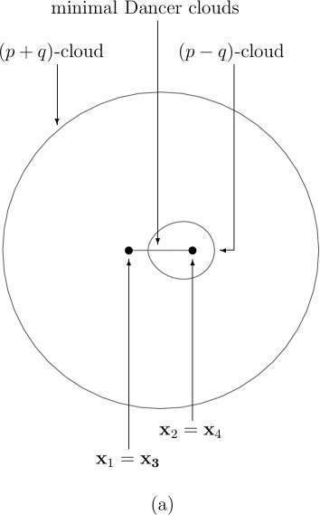
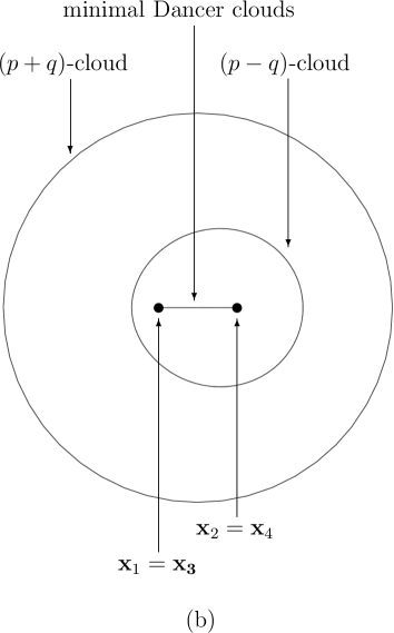
FIG. 3.: Schematic illustration of a solution with minimal Dancer clouds and coincident massive monopoles, as discussed in Subsec. VI A 2. In both figures the $(p+q)$-cloud is roughly defined by the curve $\lambda_{+}=1$ with $p+q=5D$ and the $(p-q)$-cloud by the curve $\lambda_{-}=1$, where in (a) $p-q=1.2D$ and in (b) $p+q=2.2D$. In each case $\alpha=4\pi/3$ and there are coincident $\mbox{\boldmath$\beta$}_{1}$- and $\mbox{\boldmath$\beta$}_{2}$-monopoles at ${\bf x}_{1}={\bf x}_{3}$ and at ${\bf x}_{2}={\bf x}_{4}$. The massless monopole locations are not shown, but calculating $Q_{NA}$ in different regions indicates that there are $\mbox{\boldmath$\gamma$}_{1}$- and $\mbox{\boldmath$\gamma$}_{3}$-monopoles on the minimal Dancer clouds, a $(\mbox{\boldmath$\gamma$}_{2}+\mbox{\boldmath$\gamma$}_{3})$-monopole on the $(p-q)$-cloud and a $(\mbox{\boldmath$\gamma$}_{1}+\mbox{\boldmath$\gamma$}_{2})$-monopole on the $(p+q)$-cloud.

3 Large SU(4) clouds

If $p+q$ and $p-q$ are both much larger than all of the $|{\bf x}_{i}-{\bf x}_{j}|$, then the first term on the right hand side of Eq. (212) dominates and $K$ is well approximated by Eq. (220) and $\hat{B}$ by Eq. (221). At short distances (all $r_{j}\ll p\pm q$), $\hat{B}$ is approximately a unit matrix and one sees the unshielded charge of Eq. (238). At much larger distances, the $r_{j}$ are all approximately equal. Equation (222) then gives

$$M^{-}\approx 2r\left(\matrix{c_{R}^{2}&c_{R}\,d_{R}&0&0\cr\cr c_{R}\,d_{R}&d_{R}^{2}&0&0\cr\cr 0&0&c_{L}^{2}&c_{L}\,d_{L}\cr\cr 0&0&c_{L}\,d_{L}&d_{L}^{2}}\right)$$ (241)

and

$${M^{+}\over 2r}\approx{\rm I}_{4}-{M^{-}\over 2r}\,.$$ (242)

(Here we have used the notation of Eq. (223), but have allowed for the possibility that the SU(2) orientations of the left and right Dancer clouds might be different.) It follows that

$$\hat{B}\approx{p-q+2r\over p-q}\,{M^{-}\over 2r}+{p+q+2r\over p+q}\,\left({\rm I}_{4}-{M^{-}\over 2r}\right)\,.$$ (243)

Because $M^{-}/2r$ is a projection operator, $\hat{B}^{-1/2}$ is easily calculated, and one obtains

$$\hat{\Phi}\approx{1\over 2r}\,U\left(\matrix{\vphantom{\Biggl{(}}\displaystyle{p-q\over p-q+2r}&0&0&0\cr\cr 0&\vphantom{\Biggl{(}}\displaystyle{p+q\over p+q+2r}&0&0\cr\cr 0&0&-\vphantom{\Biggl{(}}\displaystyle{p-q\over p-q+2r}&0\cr\cr 0&0&0&-\vphantom{\Biggl{(}}\displaystyle{p+q\over p+q+2r}}\right)U^{-1}$$ (244)

where $U$ is a unitary matrix that diagonalizes $M^{-}$. Hence, the non-Abelian magnetic charge is completely shielded for $r\gg p+q$, partially shielded, as in Eq. (240), for $p+q\gg r\gg p-q$, and unshielded for $r\ll p-q$.

B Two large Dancer clouds

We now consider the case where both Dancer clouds are large. For convenience, we choose our spatial axes so that the “left cloud”, corresponding to the Nahm data ${\bf T}^{L}(s)$, is centered at $(0,0,-R/2)$ and the “right cloud”, obtained from ${\bf T}^{R}(s)$ is centered at $(0,0,R/2)$. We denote the distances from these two centers by $r_{L}$ and $r_{R}$. The cloud parameters for the two clouds are $a_{L}$ and $a_{R}$, while the SU(2) orientations for the two clouds are encoded in the rotated triplets of Pauli matrices $\mbox{\boldmath$\tau$}^{L}$ and $\mbox{\boldmath$\tau$}^{R}$.

The matrix $K$ is then

$$K=[p{\rm I}_{2}+{\bf q}\cdot\mbox{\boldmath$\tau$}]\otimes{\rm I}_{2}+R{\rm I}_{2}\otimes\sigma_{3}+{a_{R}}\,\tau^{R}_{i}\otimes\sigma_{i}+{a_{L}}\,\tau^{L}_{i}\otimes\sigma_{i}\,.$$ (245)

The SU(4) cloud parameters $p$ and $\bf q$ must be such that the eigenvalues of $K$ are all positive. We will write $q=|{\bf q}|$.

Three special cases are particularly easy to analyze:

1) Large SU(4) cloud: $p\pm q\gg R,\,a_{L},\,a_{R}$.

2) Widely separated Dancer clouds: $R\gg a_{L},\,a_{R}$.

3) Two concentric large Dancer clouds: $a_{R}\gg a_{L}$, with $R=0$.

1 Large SU(4) cloud

The eigenvalues of $K$ are

$$\lambda_{1} = p+q+O(R,a_{L},a_{R})$$ (246)

$$\lambda_{2} = p+q+O(R,a_{L},a_{R})$$ (247)

$$\lambda_{3} = p-q+O(R,a_{L},a_{R})$$ (248)

$$\lambda_{4} = p-q+O(R,a_{L},a_{R})\,.$$ (249)

Our assumption that $p\pm q\gg R,\,a_{L},\,a_{R}$ ensures that these eigenvalues are all positive.

If $r\ll p-q$, the various $\hat{V}^{0}_{a}$ are of order $\sqrt{r_{R}}$, $\sqrt{r_{L}}$, $\sqrt{a_{R}}$, or $\sqrt{a_{L}}$, depending on whether $\bf r$ is outside or inside a Dancer cloud. Because these are all small compared to the eigenvalues of $K$, the second term in Eq. (205) can be neglected, $\hat{B}\approx{\rm I}_{4}$ and $\hat{\Phi}$ is a composite of two Dancer fields. If instead $r\gg p-q$, then $\bf r$ is well outside both Dancer clouds and the $\hat{V}^{0}_{a}$ are all insensitive to the SU(2) orientation of the Dancer clouds. We can, therefore, orient the SU(4) cloud parameters so that ${\bf q}=(0,0,q)$ (thus making $K$ diagonal) and at the same time choose

$$\hat{V}^{0}_{1} \approx \sqrt{2r}\left(\begin{array}[]{c}\bar{\psi}({\bf r})\\ 0\end{array}\right)\qquad\qquad\hat{V}^{0}_{2}\approx\sqrt{2r}\left(\begin{array}[]{c}0\\ \bar{\psi}({\bf r})\end{array}\right)$$ (254)

$$\hat{V}^{0}_{3} \approx \sqrt{2r}\left(\begin{array}[]{c}\psi({\bf r})\\ 0\end{array}\right)\qquad\qquad\hat{V}^{0}_{4}\approx\sqrt{2r}\left(\begin{array}[]{c}0\\ \psi({\bf r})\end{array}\right)\,.$$ (261)

(We have used the fact that $r_{L}\approx r_{R}$ in this region.) To leading approximation, this makes $\hat{B}$ diagonal. Since $\hat{\phi}$ is also diagonal outside the Dancer clouds,

$$\hat{\Phi}\approx{1\over 2r}\left(\matrix{\vphantom{\Biggl{(}}\displaystyle{p-q\over p-q+2r}&0&0&0\cr\cr 0&\vphantom{\Biggl{(}}\displaystyle{p+q\over p+q+2r}&0&0\cr\cr 0&0&-\vphantom{\Biggl{(}}\displaystyle{p-q\over p-q+2r}&0\cr\cr 0&0&0&-\vphantom{\Biggl{(}}\displaystyle{p+q\over p+q+2r}}\right)\,.$$ (262)

Thus, there are effectively two SU(4) clouds, one at $r\approx p+q$ and one at $r\approx p-q$. In the region outside both clouds, there are no non-Abelian Coulomb magnetic fields. In the intermediate region between the two clouds, the field corresponds to a non-Abelian magnetic charge

$$Q_{NA}=\rm{diag}\,(0,-1,0,1)\,.$$ (263)

In the region inside the inner SU(4) cloud, but still outside the two Dancer clouds, the fields correspond to

$$Q_{NA}=\rm{diag}\,(-1,-1,1,1)\,.$$ (264)

2 Widely separated Dancer clouds

If $R\gg a_{L},a_{R}$, the eigenvalues of $K$ are

$$\lambda_{1} = p+q+R+O(a_{L},a_{R})$$ (265)

$$\lambda_{2} = p+q-R+O(a_{L},a_{R})$$ (266)

$$\lambda_{3} = p-q+R+O(a_{L},a_{R})$$ (267)

$$\lambda_{4} = p-q-R+O(a_{L},a_{R})\,.$$ (268)

In order that these all be positive, $p\pm q\geq R$ [up to $O(a_{L},a_{R})$ corrections], which implies that $\lambda_{1},\,\lambda_{3}\geq 2R$.

If the SU(2) basis is chosen so that ${\bf q}=(0,0,q)$, then, up to $O(a_{L},a_{R})$ corrections, $K$ is diagonal with

$$K^{-1}={\rm diag}\,\left({1\over\lambda_{1}},{1\over\lambda_{2}},{1\over\lambda_{3}},{1\over\lambda_{4}}\right)\,.$$ (269)

In the region outside both Dancer clouds ($r_{R}\gg a_{R}$, $r_{L}\gg a_{L}$), the SU(2) orientation of the Dancer clouds is irrelevant and we can take

$$\hat{V}^{0}_{1} \approx \sqrt{2r_{R}}\left(\begin{array}[]{c}\bar{\psi}({\bf r}_{R})\\ 0\end{array}\right)\qquad\qquad\hat{V}^{0}_{2}\approx\sqrt{2r_{R}}\left(\begin{array}[]{c}0\\ \bar{\psi}({\bf r}_{R})\end{array}\right)$$ (274)

$$\hat{V}^{0}_{3} \approx \sqrt{2r_{L}}\left(\begin{array}[]{c}\psi({\bf r}_{L})\\ 0\end{array}\right)\qquad\qquad\hat{V}^{0}_{4}\approx\sqrt{2r_{L}}\left(\begin{array}[]{c}0\\ \psi({\bf r}_{L})\end{array}\right)\,.$$ (281)

Examining the factors that enter into $\hat{B}$, we see that it is composed of two interlocking $2\times 2$ blocks. One (containing the 11-, 13-, 31-, and 33-elements) is of the form of Eq. (125) that we encountered in the construction of the SU(4) $(1,[1],1)$ solution, except that the cloud parameter is now $p+q$. The other (lying in the second and fourth rows and columns) is similar, except with cloud parameter $p-q$.

Now consider the region inside one of the Dancer clouds. Choosing the right cloud, for definiteness, we have ${\bf r}_{L}\approx(0,0,R)$. The two $\hat{V}^{0}_{a}$ from the right-hand construction problem are

$$\hat{V}^{0}_{1}=O(r_{R}/\sqrt{a_{R}})\qquad\qquad\hat{V}^{0}_{2}\approx\sqrt{2a_{R}}\left(\begin{array}[]{c}g\\ -f\\ f^{*}\\ g^{*}\end{array}\right)$$ (282)

where, as in Eq. (169), $f$ and $g$ are elements of the SU(2) matrix that relates the $\mbox{\boldmath$\tau$}^{R}$ to the standard set of $\tau$. Since this region is well outside the left Dancer cloud, the SU(2) orientation of that cloud is irrelevant and the remaining $\hat{V}^{0}_{a}$ can be taken to be

$$\hat{V}^{0}_{3} \approx \sqrt{2R}\left(\begin{array}[]{c}\psi({\bf r}_{L})\\ 0\end{array}\right)\approx\sqrt{2R}\left(\begin{array}[]{c}1\\ O(a_{L}/R,a_{R}/R)\\ 0\\ 0\end{array}\right)$$ (289)

$$\hat{V}^{0}_{4} \approx \sqrt{2R}\left(\begin{array}[]{c}0\\ \psi({\bf r}_{L})\end{array}\right)\approx\sqrt{2R}\left(\begin{array}[]{c}0\\ 0\\ 1\\ O(a_{L}/R,a_{R}/R)\end{array}\right)\,.$$ (297)

We now use the facts that $\lambda_{1}^{-1}$ and $\lambda_{3}^{-1}$ are at most $O(1/R)$ and that $\lambda_{2}^{-1}$ and $\lambda_{4}^{-1}$ can be at most $O(1/a_{R})$ before our approximations break down. Together with the above expressions for the $\hat{V}^{0}_{a}$, these imply that all the elements of $\hat{B}_{ab}$ are of order unity or smaller. In fact, the off-diagonal elements are $O(\sqrt{a_{R}/R})$, except for $\hat{B}_{12}=(\hat{B}_{21})^{*}=O(r_{R}/a_{R})$. Hence, there is no significant modification of the Dancer Higgs fields inside the Dancer cloud.

The results of this analysis are summarized in Fig. 4, where we indicate the regions delineated by the various clouds and show the value of $Q_{NA}$ in each.

FIG. 4.: Schematic illustration of a solution with two widely-separated large Dancer clouds. The clouds are labelled both by the relevant distance scale and by the associated massless monopole. The diagonal elements of $Q_{NA}$, which is assumed to be a diagonal matrix, are shown for each of the regions defined by the clouds.

3 Two concentric large Dancer clouds

We now consider two concentric Dancer clouds, with $a_{R}\equiv a\gg a_{L}$. Without loss of generality, we can choose the SU(2) orientation of the right Dancer cloud so that the $\mbox{\boldmath$\tau$}^{R}$ are the standard Pauli $\tau$. The orientation of the SU(4) cloud, encoded in $\bf q$, and of the left Dancer cloud are arbitrary; the orientation of the latter will actually play no role in our considerations. Finally, because these solutions are spherically symmetric, it is sufficient to examine the fields along the positive $z$-axis.

The matrix $K$ is

$$K\approx[p{\rm I}_{2}+{\bf q}\cdot\mbox{\boldmath$\tau$}]\otimes{\rm I}_{2}+{a_{R}}\,\tau^{R}_{i}\otimes\sigma_{i}\,.$$ (298)

To leading order, its eigenvalues (although not its eigenvectors) are independent of the direction of $\bf q$. They are

$$\lambda_{1} = p+q+{a}+O(a_{L})$$ (299)

$$\lambda_{2} = p-{a}+\sqrt{4a^{2}+q^{2}}+O(a_{L})$$ (301)

$$\lambda_{3} = p-q+{a}+O(a_{L})$$ (303)

$$\lambda_{4} = p-{a}-\sqrt{4a^{2}+q^{2}}+O(a_{L})\,.$$ (305)

These obey $\lambda_{1}\geq\lambda_{2}\geq\lambda_{3}>\lambda_{4}$, with the first two relations being equalities only if $q=0$. Note that the last relation can never be an equality, so only $\lambda_{4}$ can vanish. Furthermore, once $p$ is chosen to make $\lambda_{4}$ positive, the remaining $\lambda_{j}$ are all $O(a)$ or larger.

We will examine separately the region well outside the Dancer cloud, $r\gg a$, and the region well inside the cloud, $r\ll a$. Outside the cloud, it is possible to choose a basis so that the $\hat{V}^{0}_{j}$ along the $z$-axis are

$$\hat{V}^{0}_{1} = \sqrt{2r}\,(0,1,0,0)^{t}$$ (306)

$$\hat{V}^{0}_{2} = \sqrt{2r}\,(0,0,0,1)^{t}$$ (308)

$$\hat{V}^{0}_{3} = \sqrt{2r}\,(1,0,0,0)^{t}$$ (310)

$$\hat{V}^{0}_{4} = \sqrt{2r}\,(0,0,1,0)^{t}\,.$$ (312)

In this basis,

$$\hat{\varphi}={1\over 2r}{\rm diag}\,(1,1,-1,-1)\,.$$ (313)

There several possibilities to consider, depending on the magnitudes of the $\lambda_{j}$. If these eigenvalues are all $O(a)$ or smaller, then in this region all of the eigenvalues of $\hat{B}$ will be $O(r/a)$ and $\hat{\Phi}$ will be $O(a/r^{2})$, corresponding to complete shielding of the non-Abelian magnetic charge. If, instead, the $\lambda_{j}$ are all much greater than $a$, the “large SU(4) cloud” analysis given above applies. There are effectively two SU(4) clouds, one of radius $p+q$ and other of radius $p-q$. The effective non-Abelian magnetic charge vanishes outside both, is given by Eq. (263) between the two, and is given by Eq. (264) for $p-q\gg r\gg a$.

The only remaining possibility is that $\lambda_{1}\approx\lambda_{2}\approx p+q\gg a$ while $\lambda_{3}$ and $\lambda_{4}$ are $O(a)$ or smaller. As before, the non-Abelian charge is completely shielded for $r\gg p+q$. In calculating the fields at shorter distance to leading order in $a/r$, we can approximate $K^{-1}$ by $\Pi K^{-1}\Pi$, where

$$\Pi\approx{{\rm I}_{2}+\hat{\bf q}\cdot\mbox{\boldmath$\tau$}\over 2}\otimes{\rm I}_{2}$$ (314)

projects onto the subspace spanned by the eigenvectors corresponding to $\lambda_{3}$ and $\lambda_{4}$. It is easy to see that by a change of basis that mixes $\hat{V}^{0}_{1}$ with $\hat{V}^{0}_{2}$ and $\hat{V}^{0}_{3}$ with $\hat{V}^{0}_{4}$ one can obtain new vectors such that $\hat{V}^{{}^{\prime}0}_{1}$ and $\hat{V}^{{}^{\prime}0}_{3}$ lie in the subspace onto which $\Pi$ projects while $\hat{V}^{{}^{\prime}0}_{2}$ and $\hat{V}^{{}^{\prime}0}_{4}$ lie in the orthogonal subspace. (This change of basis leaves Eq. (313) unchanged.) In this basis $\hat{B}$ is approximately the identity in the 2-4 subspace, but has two large eigenvalues (of order $r/a$) in the 1-3 subspace. As a result, two of the eigenvalues of the Higgs field are shielded, so that the only large components are in the 2-4 subspace and the effective magnetic charge is given by Eq. (263).

We now turn to the region well inside the Dancer cloud, $r\ll a$, although still with $r\gg a_{L}$. To leading order in $r/a$ the $\hat{V}^{0}_{j}$ along the positive $z$-axis can be taken to be

$$\hat{V}^{0}_{1} = \sqrt{2r}\,(0,0,0,1)^{t}$$ (315)

$$\hat{V}^{0}_{2} = \sqrt{2a}\,(0,-1,1,0)^{t}$$ (317)

$$\hat{V}^{0}_{3} = \sqrt{2r}\,(1,0,0,0)^{t}$$ (319)

$$\hat{V}^{0}_{4} = \sqrt{2r}\,(0,0,1,0)^{t}$$ (321)

while to the same order

$$\hat{\varphi}={1\over 2r}{\rm diag}\,(2,0,-1,-1)\,.$$ (322)

If all of the $\lambda_{j}$ are $O(a)$ or larger, then $\hat{B}\approx I$ in this region and there is no shielding of non-Abelian magnetic charge. The only other possibility is that $\lambda_{4}\equiv\Delta\ll a$, with the remaining $\lambda_{j}$ being at least $O(a)$. We now examine this second case. Let $u$ be the eigenvector of $K$ with eigenvalue $\lambda_{4}$, and define $w_{j}=u^{\dagger}\hat{V}^{0}_{j}$. Using the above expressions for the $\hat{V}^{0}_{j}$, we have

$$\hat{B}_{ij}=\delta_{ij}+{1\over\Delta}w_{i}^{\dagger}w_{j}+c\,\delta_{i2}\delta_{j2}+O(\sqrt{r/a})$$ (323)

where $c$ is of order unity. Next, note that $w_{2}$ is larger than the other $w_{j}$ by a factor of order $\sqrt{r/a}$ that arises from the relative magnitudes of the $\hat{V}^{0}_{j}$. Hence, to leading order the term containing $c$ can be included in the $w_{i}^{\dagger}w_{j}$ term, giving

$$\hat{B}_{ij}=\delta_{ij}+{(1+c\,\Delta)\over\Delta}w_{i}^{\dagger}w_{j}+O(\sqrt{r/a})\,.$$ (324)

Inverting this matrix gives

$$(\hat{B}^{-1})_{ij} = \delta_{ij}-{w_{i}^{\dagger}w_{j}\over|w|^{2}}+{\Delta\,w_{i}^{\dagger}w_{j}\over(1+c\,\Delta)|w|^{4}}+O(\sqrt{r/a})$$ (325)

$$= \delta_{ij}-\delta_{i2}\delta_{j2}+O(\sqrt{r/a})$$ (327)

where $|w|^{2}=w_{i}^{\dagger}w_{i}$. Recalling the vanishing of $\hat{\varphi}_{22}$ in Eq. (322), we see that to leading order in $r/a$ there is no modification of the Higgs field.

It is straightforward to extend this analysis to the region, $r\ll a_{L}$, inside the smaller cloud and to show that to leading order the SU(4) clouds do not modify the Higgs field there. This result does not depend on the relative SU(2) orientation of the two Dancer clouds.

FIG. 5.: Schematic illustration of a solution with two concentric large Dancer clouds. The clouds are labelled both by the relevant distance scale and by the associated massless monopole. The diagonal elements of $Q_{NA}$, which is assumed to be a diagonal matrix, are shown for each of the regions defined by the clouds.

To summarize, we can distinguish five concentric regions (four, if $p-q\sim a_{R}$). The effective magnetic charges seen within these are

$$Q_{NA}=\cases{{\rm diag}\,(0,0,0,0)\,,&$r\gg p+q$\cr\cr{\rm diag}\,(0,-1,0,1)\,,&$p+q\gg r\gg{\rm Max}(p-q,a_{R})$\cr\cr{\rm diag}\,(-1,-1,1,1)\,,&$p-q\gg r\gg a_{R}$\cr\cr{\rm diag}\,(-2,0,1,1)\,,&$a_{R}\gg r\gg a_{L}$\cr\cr{\rm diag}\,(-2,0,0,2)\,,&$a_{L}\gg r$ \, .}$$ (328)

We illustrate this in Fig. 5.

VII Clouds and massless monopoles

With the explicit examples of the previous section in hand, we can now examine more closely the relationship between the massless monopoles and the non-Abelian clouds. The first thing to notice is that there are six massless monopoles but only four non-Abelian clouds. In other words, the number of distinct clouds evident in the solutions is less than the number of massless monopoles obtained by adding the coefficients of the $\gamma_{a}$ in Eq. (4). The number of degrees of freedom in the SU(6) $(2,[2],[2],[2],2)$ solutions, 40, is precisely that expected when there are a total of ten (four massive and six massless) monopoles. However, in all the examples we have studied, these degrees of freedom parameterize the four massive monopoles and only four distinct, though sometimes degenerate, clouds. In other words, there is not a one-to-one correspondence between clouds and massless monopoles. We expect that the solutions we have studied are not exceptional in this regard and that a general $(2,[2],[2],[2],2)$ will have four clouds.

To help understand this, recall that requiring that ${\bf h}\cdot\mbox{\boldmath$\beta$}_{a}$ is positive determines a unique set of simple roots when the symmetry is maximally broken, but when the unbroken group has a non-Abelian factor ${\bf h}\cdot\mbox{\boldmath$\beta$}_{a}=0$ for some $\mbox{\boldmath$\beta$}_{a}$’s and so there are a number of possible choices for the simple roots, all related by Weyl transformations. To be specific, let us consider SU(6). Following Fig. 1, we denote the simple roots for the maximally broken case by $\mbox{\boldmath$\beta$}_{1}$, $\mbox{\boldmath$\gamma$}_{1}$, $\mbox{\boldmath$\gamma$}_{2}$, $\mbox{\boldmath$\gamma$}_{3}$, and $\mbox{\boldmath$\beta$}_{2}$. Each of these corresponds to a massive fundamental monopole. In the limit where the unbroken symmetry is enlarged to U(1)$\times$SU(4)$\times$U(1), the $\mbox{\boldmath$\beta$}_{1}$-monopole becomes part of a multiplet of degenerate states transforming as a 4 of SU(4); the remaining states in this multiplet correspond to the roots $(\mbox{\boldmath$\beta$}_{1}+\mbox{\boldmath$\gamma$}_{1})$, $(\mbox{\boldmath$\beta$}_{1}+\mbox{\boldmath$\gamma$}_{1}+\mbox{\boldmath$\gamma$}_{2})$, and $(\mbox{\boldmath$\beta$}_{1}+\mbox{\boldmath$\gamma$}_{1}+\mbox{\boldmath$\gamma$}_{2}+\mbox{\boldmath$\gamma$}_{3})$, all of which can be obtained from $\mbox{\boldmath$\beta$}_{1}$ by Weyl transformations. Similarly, the $\mbox{\boldmath$\beta$}_{2}$-monopole is part of a $\bar{\bf 4}$ that also includes the $(\mbox{\boldmath$\beta$}_{2}+\mbox{\boldmath$\gamma$}_{3})$-, $(\mbox{\boldmath$\beta$}_{2}+\mbox{\boldmath$\gamma$}_{3}+\mbox{\boldmath$\gamma$}_{2})$-, and $(\mbox{\boldmath$\beta$}_{2}+\mbox{\boldmath$\gamma$}_{3}+\mbox{\boldmath$\gamma$}_{2}+\mbox{\boldmath$\gamma$}_{1})$-monopoles. Clearly, the straightforward correspondence of simple roots with elementary monopoles and composite roots with multimonopoles has become more complicated.

It is useful to make a detailed correspondence between the clouds and the massless monopoles in specific solutions. This can be done by noting the effect of each cloud on the non-Abelian charge $Q_{NA}$. Recall that the non-Abelian charges of the massive $\mbox{\boldmath$\beta$}_{1}$- and $\mbox{\boldmath$\beta$}_{2}$-monopoles are

$$Q_{NA}(\mbox{\boldmath$\beta$}_{1}) = {\rm diag}\,(-1,0,0,0)$$ (329)

$$Q_{NA}(\mbox{\boldmath$\beta$}_{2}) = {\rm diag}\,(0,0,0,1)$$ (330)

while those of the massless monopoles are

$$Q_{NA}(\mbox{\boldmath$\gamma$}_{1})={\rm diag}\,(1,-1,0,0)$$ (331)

$$Q_{NA}(\mbox{\boldmath$\gamma$}_{2})={\rm diag}\,(0,1,-1,0)$$ (332)

$$Q_{NA}(\mbox{\boldmath$\gamma$}_{3})={\rm diag}\,(0,0,1,-1)$$ (333)

$$Q_{NA}(\mbox{\boldmath$\gamma$}_{1}+\mbox{\boldmath$\gamma$}_{2})={\rm diag}\,(1,0,-1,0)$$ (334)

$$Q_{NA}(\mbox{\boldmath$\gamma$}_{2}+\mbox{\boldmath$\gamma$}_{3})={\rm diag}\,(0,1,0,-1)$$ (335)

$$Q_{NA}(\mbox{\boldmath$\gamma$}_{1}+\mbox{\boldmath$\gamma$}_{2}+\mbox{\boldmath$\gamma$}_{3})={\rm diag}\,(1,0,0,-1)$$ (336)

where we have listed the charges for all of the massless positive roots, not just the $\mbox{\boldmath$\gamma$}_{a}$.

As an example, consider the case of concentric Dancer clouds illustrated in Fig. 5 and described by Eq. (328). In the innermost region, $r\ll a_{L}$, we have the field due to two $\mbox{\boldmath$\beta$}_{1}$- and two $\mbox{\boldmath$\beta$}_{2}$-monopoles. Moving outward, we find a $\mbox{\boldmath$\gamma$}_{3}$-monopole at $r\approx a_{L}$, a $\mbox{\boldmath$\gamma$}_{1}$-monopole at $r\approx a_{R}$, a $(\mbox{\boldmath$\gamma$}_{1}+\mbox{\boldmath$\gamma$}_{2})$-monopole at $r\approx p-q$ and finally a $(\mbox{\boldmath$\gamma$}_{2}+\mbox{\boldmath$\gamma$}_{3})$-monopole at $r\approx p+q$.

The fact that two of these roots are simple and two are composite is a gauge-dependent statement; the sequence $\mbox{\boldmath$\gamma$}_{3}$, $\mbox{\boldmath$\gamma$}_{1}$, $\mbox{\boldmath$\gamma$}_{2}$, $(\mbox{\boldmath$\gamma$}_{1}+\mbox{\boldmath$\gamma$}_{2}+\mbox{\boldmath$\gamma$}_{3})$, for example, leads to a physically equivalent configuration. However, the sum of these roots, $2\mbox{\boldmath$\gamma$}_{1}+2\mbox{\boldmath$\gamma$}_{2}+2\mbox{\boldmath$\gamma$}_{3}$, (corresponding to a total of six massless monopoles) is invariant, as is the fact that two of the roots are “Dancer roots” that are orthogonal to one $\mbox{\boldmath$\beta$}_{a}$ but not to the other. We can also apply a gauge transformation that replaces one of the $\mbox{\boldmath$\beta$}_{a}$ by a compound root. Such a transformation will replace some of the positive roots in the above sequences by a negative roots, but the sum of the coefficients of the $\mbox{\boldmath$\gamma$}_{a}$ will remain unchanged. The correspondence between monopoles and clouds for various solutions is indicated in Figs. 2-5.

Let us try to develop some rules to explain how and where the various massless monopoles can appear in these solutions. It is useful to begin by discussing what happens to the $\mbox{\boldmath$\gamma$}_{a}$-monopoles in the maximally broken theory when the Higgs expectation value $\Phi_{0}$ is varied. As $\Phi_{0}$ approaches a value with an enlarged symmetry group, the masses of some of the elementary bosons decrease, eventually vanishing in the limit where the symmetry becomes non-Abelian. For an isolated $\mbox{\boldmath$\gamma$}_{a}$-monopole, the core radius is inversely proportional to the corresponding elementary boson mass and so grows monotonically and becomes infinite in the non-Abelian limit. Similarly, for a configuration composed of two monopoles, a $\mbox{\boldmath$\gamma$}_{1}$-monopole and a $\mbox{\boldmath$\gamma$}_{2}$-monopole, for example, the component monopoles each grow without bound as the corresponding masses vanish. When their core radii are much larger than the separation of their centers, the two-monopole configuration is barely distinguishable from a gauge-transformed one-monopole solution.

However, the situation can be different if the configuration contains a monopole that remains massive in the non-Abelian limit. If the fields in the massive core transform under the non-Abelian symmetry, some of the massless gauge fields acquire an effective mass near the massive core. This can dramatically modify the behavior of the massless monopole cores. There are three possible situations. One possibility is that the massive and massless monopoles lie in mutually commuting subgroups. The massive monopole then has no effect on the massless monopole, and the behavior described in the previous paragraph is unchanged. Another possibility is that the addition of the massless monopole to the massive monopole corresponds to a gauge transformation of the massive monopole, in which case no gauge-invariant evidence of the massless monopole survives in the non-Abelian limit. The most interesting case is when neither of these holds. The massless monopole core then expands only until it reaches the massive monopole, resulting in a cloud whose radius is equal to the original intermonopole separation.

A similar pattern should be expected when several massive monopoles are present. A massless monopole with non-Abelian charge $q$ should be able to form a finite size cloud enclosing a collection of monopoles with total charge $Q_{NA}$ only if (1) $q$ does not lie in the subgroup that leaves $Q_{NA}$ invariant and (2) $Q_{NA}^{\prime}=Q_{NA}+q$ is not gauge-equivalent to $Q_{NA}$. This is consistent with the behavior of the clouds in both the SU(3) Dancer and the SU(4) $(1,[1],1)$ solutions. In each case, combining the massless monopole with just one of the massive monopoles would simply give a gauge-transformed massive monopole and, indeed, we only find solutions where the cloud encloses both of the massive monopoles.

Let us apply these rules to the concentric Dancer cloud solutions of Sec. VI B 3. We start with two $\mbox{\boldmath$\beta$}_{1}$- and two $\mbox{\boldmath$\beta$}_{2}$-monopoles, with a total non-Abelian charge

$$Q_{1}=2Q_{NA}(\mbox{\boldmath$\beta$}_{1})+2Q_{NA}(\mbox{\boldmath$\beta$}_{2})={\rm diag}\,(-2,0,0,2)\,,$$ (337)

and want to add one of the massless monopoles whose charges were enumerated in Eq. (336). There are four possibilities: we can add a massless monopole corresponding to:

1. $\mbox{\boldmath$\gamma$}_{1}$ or $(\mbox{\boldmath$\gamma$}_{1}+\mbox{\boldmath$\gamma$}_{2})$; these give gauge-equivalent solutions in the $Q_{1}$ background.

2. $\mbox{\boldmath$\gamma$}_{3}$ or $(\mbox{\boldmath$\gamma$}_{2}+\mbox{\boldmath$\gamma$}_{3})$; these are similarly gauge-equivalent.

3. $\mbox{\boldmath$\gamma$}_{2}$.

4. $(\mbox{\boldmath$\gamma$}_{1}+\mbox{\boldmath$\gamma$}_{2}+\mbox{\boldmath$\gamma$}_{3})$.

Cases (a) and (b) differ only by the interchange of the left and right Dancer solutions, and need not be considered separately. Case (c) is ruled out because $\mbox{\boldmath$\gamma$}_{2}$ lies in the SU(2) subgroup that leaves Eq. (337) invariant. Thus, it is sufficient to consider cases (b) and (d). We start with the former, and add a $\mbox{\boldmath$\gamma$}_{3}$-monopole to get

$$Q_{2}=Q_{1}+Q_{NA}(\mbox{\boldmath$\gamma$}_{3})={\rm diag}\,(-2,0,1,1)\,.$$ (338)

The possible choices for the next massless monopole are:

1. $\mbox{\boldmath$\gamma$}_{1}$.

2. $(\mbox{\boldmath$\gamma$}_{1}+\mbox{\boldmath$\gamma$}_{2})$ or $(\mbox{\boldmath$\gamma$}_{1}+\mbox{\boldmath$\gamma$}_{2}+\mbox{\boldmath$\gamma$}_{3})$; these are gauge-equivalent to each other.

3. $\mbox{\boldmath$\gamma$}_{3}$; this is ruled out because it lies in the SU(2) symmetry group of Eq. (338).

4. $\mbox{\boldmath$\gamma$}_{2}$ or $(\mbox{\boldmath$\gamma$}_{2}+\mbox{\boldmath$\gamma$}_{3})$; these just gauge transform $Q_{2}$, [e.g., $Q_{2}+Q_{NA}(\mbox{\boldmath$\gamma$}_{2})={\rm diag}\,(-2,1,0,1)$] and so cannot give rise to a cloud.

Once more, we have two acceptable choices, (a) and (b). If we take the former, we obtain

$$Q_{3}=Q_{2}+Q_{NA}(\mbox{\boldmath$\gamma$}_{1})={\rm diag}\,(-1,-1,1,1)\,.$$ (339)

We cannot add either a $\mbox{\boldmath$\gamma$}_{1}$- or a $\mbox{\boldmath$\gamma$}_{3}$-monopole to this, since both lie in the SU(2)$\times$SU(2) symmetry group of $Q_{3}$. The remaining four possibilities are all gauge-equivalent. Choosing $(\mbox{\boldmath$\gamma$}_{1}+\mbox{\boldmath$\gamma$}_{2})$, we obtain

$$Q_{4}=Q_{3}+Q_{NA}(\mbox{\boldmath$\gamma$}_{1}+\mbox{\boldmath$\gamma$}_{2})={\rm diag}\,(0,-1,0,1)\,.$$ (340)

At this point, the remaining massless monopoles only allow three possibilities: $\mbox{\boldmath$\gamma$}_{2}$, $\mbox{\boldmath$\gamma$}_{3}$, and $(\mbox{\boldmath$\gamma$}_{2}+\mbox{\boldmath$\gamma$}_{3})$. The first two are excluded because they give gauge transforms of $Q_{4}$. The third gives

$$Q_{5}=Q_{4}+Q_{NA}(\mbox{\boldmath$\gamma$}_{2}+\mbox{\boldmath$\gamma$}_{3})={\rm diag}\,(0,0,0,0)\,.$$ (341)

We therefore recover the sequence $\mbox{\boldmath$\gamma$}_{3}$, $\mbox{\boldmath$\gamma$}_{1}$, $(\mbox{\boldmath$\gamma$}_{1}+\mbox{\boldmath$\gamma$}_{2})$, $(\mbox{\boldmath$\gamma$}_{2}+\mbox{\boldmath$\gamma$}_{3})$ that we found previously.

We now must return to the alternatives that we did not follow. At the first step, we could have taken case (d) and added a $(\mbox{\boldmath$\gamma$}_{1}+\mbox{\boldmath$\gamma$}_{2}+\mbox{\boldmath$\gamma$}_{3})$-monopole to $Q_{1}$, thus reaching in one step a charge that was gauge-equivalent to $Q_{4}$. This can be viewed as simply a degenerate case of the four-step sequence, corresponding to the situation where $a_{L}=a_{R}=p-q$. The other place where we had an option was in adding on to $Q_{2}$, where we could have followed case (b) and added a $(\mbox{\boldmath$\gamma$}_{1}+\mbox{\boldmath$\gamma$}_{2})$-monopole. Once again, this is simply a degenerate case, equivalent to taking $a_{R}=p-q$.

Another instructive example is the solution with two minimal Dancer clouds that was analyzed in Sec. VI A 1 and illustrated in Fig. 2. The two $\mbox{\boldmath$\beta$}_{1}$-monopoles “anchor” a massless monopole corresponding (by a gauge choice) to $(\mbox{\boldmath$\gamma$}_{1}+\mbox{\boldmath$\gamma$}_{2})$. In this solution the corresponding ellipsoidal Dancer cloud has degenerated into a line, and the fields are those appropriate to two massive monopoles, one with non-Abelian charge

$$Q_{NA}(\mbox{\boldmath$\beta$}_{1})=\rm diag\,(-1,0,0,0)$$ (342)

at ${\bf x}_{1}$, and one with

$$Q_{NA}(\mbox{\boldmath$\beta$}_{1}+\mbox{\boldmath$\gamma$}_{1}+\mbox{\boldmath$\gamma$}_{2})=\rm diag\,(0,0,-1,0)$$ (343)

at ${\bf x}_{2}$. Similarly, a $(\mbox{\boldmath$\gamma$}_{2}+\mbox{\boldmath$\gamma$}_{3})$-monopole forms a minimal Dancer cloud about the $\mbox{\boldmath$\beta$}_{2}$-monopoles, effectively yielding a pair of massive monopoles with charges $\rm diag\,(0,1,0,0)$ (at ${\bf x}_{3}$) and $\rm diag\,(0,0,0,1)$ (at ${\bf x}_{4}$). At this point we are left with only two massless monopoles, a $\mbox{\boldmath$\gamma$}_{1}$ and a $\mbox{\boldmath$\gamma$}_{3}$. The former can form a cloud anchored by the monopoles at ${\bf x}_{1}$ and ${\bf x}_{3}$, whose total charge is $\rm diag\,(-1,1,0,0)=-Q_{NA}(\mbox{\boldmath$\gamma$}_{1})$. It could not, on the other hand, have formed a cloud about the ${\bf x}_{1}$- and ${\bf x}_{4}$- or the ${\bf x}_{2}$- and ${\bf x}_{3}$-monopoles, because in each case the effect of the $\mbox{\boldmath$\gamma$}_{1}$-monopole would have only been to gauge transform the sum of the charges of the two massive monopoles. By similar arguments, the $\mbox{\boldmath$\gamma$}_{3}$-monopole can only condense about the monopoles at ${\bf x}_{2}$ and ${\bf x}_{4}$.

Similar analyses can be applied to the other limiting cases studied in Sec. VI. In all cases, the appearance of the massless monopoles and their clouds is consistent with the rules outlined above.

VIII Summary and concluding remarks

Our goal in this paper has been to gain further insight into the massless monopoles that can arise when a gauge theory is spontaneously broken to a subgroup containing a non-Abelian factor. These can be viewed as limiting cases of massive fundamental monopoles of the maximally broken theory, in the sense that they have the same number of degrees of freedom and that the moduli space metric describing their dynamics is a smooth limit of that for the maximally broken case. In contrast to the massive fundamental monopoles, however, they cannot be realized as isolated classical solutions. Instead, they are manifested through non-Abelian clouds surrounding one or more massive monopoles. We have focussed on the $(2,[2],\dots,[2],2)$ solutions of SU($N$) broken to U(1)$\times$SU($N-2$)$\times$U(1). These solutions display a much richer structure than the one-cloud solutions that have been previously studied. The case of $N=6$ is generic, in the sense that the solutions for $N>6$ can all be obtained by embedding the SU(6) solution; we will discuss the restriction to smaller groups, and in particular SU(4), below.

We have used the Nahm construction to obtain these solutions. A crucial ingredient in the application of this construction is the fact that the Nahm data for the SU(6) problem are equivalent to two sets of SU(3) Dancer Nahm data, together with a set of constant jump data. In the particular case where the jump data are large compared to the other scales in the problem, they define a pair of nested “SU(4) clouds” that enclose two independent Dancer solutions, characterized by Dancer cloud parameters $a_{L}$ and $a_{R}$.

The spacetime fields of the SU(6) solution can be obtained from those of the related Dancer solutions by purely algebraic manipulations. Although the Dancer fields are not explicitly known for arbitrary parameters, analytic approximations can be obtained both in the limit where $a$ is much greater than the separation of the massive monopoles and in the case of minimal Dancer cloud. Using these approximations, we have obtained the leading behavior of the SU(6) solutions for a number of limiting cases.

In these solutions, the clouds divide space into distinct regions, each of which can be characterized by a non-Abelian magnetic charge $Q_{NA}$. By comparing the values of $Q_{NA}$ in adjacent regions, one can establish a correspondence between a specific cloud and a particular massless monopole. In each case, one or more clouds are associated with massless monopoles corresponding to compound, rather than simple, roots. As a result, the number of fundamental massless monopoles (as defined, e.g., by the counting of degrees of freedom), which is obtained by adding the coefficients of the simple roots in Eq. (4), is greater than the number of distinct clouds. The SU(6) solutions contain six massless monopoles but only four clouds, of which two are inherited from the Dancer solutions and two are SU(4) clouds associated with the jump data.

Our explicit solutions also help clarify the role of the parameters that enter the general $(2,[2],[2],[2],2)$ solution. The moduli space is 40-dimensional, with 17 of these corresponding to the unbroken U(1)$\times$SU(4)$\times$U(1) symmetry. The remaining 23 parameters were enumerated at the end of Sec. III. Twelve of these specify the positions of the massive monopoles, and two others give the relative U(1) phase between pairs of identical massive monopoles. As with the U(1) phase parameter in the SU(2) two-monopole solution, the effect of these phases falls exponentially with the monopole separation. They have, therefore, played no role in our analysis, which focussed on the region outside of the massive monopole cores.

The remaining nine parameters are associated with the non-Abelian clouds. Roughly speaking, four of these ($a_{L}$, $a_{R}$, $p$, and $q$) are cloud size parameters and five determine the relative SU(2) orientations of the Dancer and SU(4) clouds. However, as the example of Sec. VI A 2 shows, this division between size and orientation parameters is not completely clearcut, since the shape of the cloud can depend upon the orientation parameters.

It is instructive to compare the SU(2) orientation parameters with the U(1) phase parameters. The latter would be true symmetry parameters, having no effect on the form of the solutions, were it not for the interactions between the U(1)-charged fields in the cores of the massive monopoles. The exponential falloff in the effect of these parameters results from the fact that fields with U(1) charge are all massive. The role of the SU(2) parameters is similar, but because there are massless fields carrying SU(2) charges, the effect of these parameters only falls as a power of distance. Note that the distance to the SU(4) cloud is crucial here, since the Dancer solutions lie in mutually commuting subgroups and therefore have no direct interactions.

It is also useful to consider the application of our results to smaller groups. In particular, let us try to identify those SU(6) solutions that can be viewed as embeddings of the $(2,[2],2)$ SU(4) solutions. In the Nahm construction, these are distinguished by the fact that their jump data includes only two independent $a_{p}$, rather than four. In terms of the construction of Sec. IV, this translates into the statement that two of the eigenvalues of $K$ vanish. A more physical characterization is based on the fact that the SU(4) solutions contain only two massless monopoles, and thus, at most, two distinct clouds. Hence, they must correspond to SU(6) solutions in which some of the clouds are coincident.

Let us apply these considerations to some of the examples discussed in Sec. VI:

1. Minimal Dancer clouds with all SU(2)’s aligned (Sec. VI A 1): There are two ways for $K$ to have two vanishing eigenvalues. One is to set $p+q=|{\bf x}_{1}-{\bf x}_{3}|$ and $p-q=|{\bf x}_{2}-{\bf x}_{4}|$. This is equivalent to a pair of SU(4) $(1,[1],1)$, each of which has a minimal cloud and is thus an SU(3) solution embedded in SU(4). The alternative is to take $p=q$ and ${\bf x}_{2}-{\bf x}_{4}$. This is equivalent to an SU(4) $(1,[1],1)$ solution, with massive monopoles at ${\bf x}_{1}$ and ${\bf x}_{3}$ and cloud size $p+q=2p$, together with a minimal cloud SU(4) $(1,[1],1)$ solution with coincident massive monopoles at ${\bf x}_{2}$.

2. Minimal Dancer clouds with coincident massive monopoles (Sec. VI A 2): Equation (220) shows that two eigenvalues of $K$ vanish if $p=q$. Equation (221) then implies that the nonvanishing components of the Higgs field must lie in the subspace orthogonal to $M^{-}$. If the angle $\alpha$ defined in Eq. (224) vanishes, this gives the second solution of case (1), but with the restriction that ${\bf x}_{1}={\bf x}_{3}$. On the other hand, if $\alpha\neq 0$, corresponding to misaligned SU(2) orientations, then the outermost cloud (specified roughly by $\lambda_{+}=1$) encloses all four of the massive monopoles.

3. Two widely separated large Dancer clouds (Sec. VI B 2): The vanishing of two of the eigenvalues in Eq. (268) implies that $p=R+O(a)$ and $q=O(a)$; a more careful analysis of Eq. (245) is needed to determine the exact values. This leads to a somewhat degenerate version of the situation depicted in Fig. 4, with the two Dancer clouds and the two SU(4) clouds not clearly distinguishable.

4. Two concentric large Dancer clouds (Sec. VI B 3): If we insist that $a_{R}\gg a_{L}$, as in our previous analysis, then at most one eigenvalue of $K$ can vanish, implying that this cannot be reduced to an SU(4) solution. On the other hand, examination of Eq. (245) suggests that there should be embedded SU(4) solutions with $a_{R}\approx a_{L}\approx p-q$. In terms of the discussion following Eq. (340), this corresponds to having the clouds from the $\mbox{\boldmath$\gamma$}_{1}$-, the $\mbox{\boldmath$\gamma$}_{3}$-, and the $(\mbox{\boldmath$\gamma$}_{1}+\mbox{\boldmath$\gamma$}_{2})$-monopoles all coincident, with the fourth, $(\mbox{\boldmath$\gamma$}_{2}+\mbox{\boldmath$\gamma$}_{3})$, cloud at a (possibly much larger) radius $p+q$.

For SU(4) broken to U(1)$\times$SU(2)$\times$U(1), a solution containing $k_{1}$ $\mbox{\boldmath$\beta$}_{1}$-monopoles and $k_{2}$ $\mbox{\boldmath$\beta$}_{2}$-monopoles has vanishing SU(2) magnetic charge, and thus no asymptotic non-Abelian Coulomb field, if there are exactly $(k_{1}+k_{2})/2$ massless $\gamma$-monopoles. However, this tells us little about the magnetic field at finite distances. In particular, we would like to know whether the massive monopoles are “paired up” to form SU(2)-neutral combinations composed of two massive monopoles enclosed by a single massless monopole cloud. It is certainly clear that configurations of this sort must exist. Thus, there should be $(2,[2],2)$ solutions that are approximately the sum of two widely separated $(1,[1],1)$ solutions, as well as others that correspond to two widely separated Dancer solutions, one formed from the $\mbox{\boldmath$\beta$}_{1}$-monopoles and one from the $\mbox{\boldmath$\beta$}_{2}$-monopoles. The question is whether this is the generic situation. The solutions described in paragraph (2) are instructive in this regard. For $\alpha=0$ these do, indeed, naturally separate into a pair of $(1,[1],1)$ solutions. However, for the presumably more generic case of nonzero $\alpha$, we find that the “$\lambda_{+}$-cloud” encloses all four massive monopoles. This strongly suggests that in general there is no clear pairing of massive monopoles.

Finally, we want to indicate briefly two areas for future research. The first is the determination of the $(2,[2],\dots,[2],2)$ moduli space metric, which determines the low-energy dynamics of the monopoles. In general, the explicit determination of such metrics is a difficult task. However, one might hope that relation between the Dancer Nahm data and the $(2,[2],\dots,[2],2)$ Nahm data could be exploited to allow a construction of the moduli space metric in terms of the Dancer metric [11]. Secondly, one would like to understand better the quantum theory of monopoles with non-Abelian charges, and in particular the complex interplay of the non-Abelian electric and magnetic charges [26]. The knowledge of classical multicloud solutions that we have gained should help provide a starting point for this investigation.

REFERENCES

• [1] C. Montonen and D. I. Olive, Phys. Lett. B 72, 117 (1977).
• [2] K. Lee, E. J. Weinberg, and P. Yi, Phys. Rev. D 54, 6351 (1996).
• [3] E. B. Bogomolny, Sov. J. Nucl. Phys.  24, 449 (1976) [Yad. Fiz.  24, 861 (1976)].
• [4] M. K. Prasad and C. M. Sommerfield, Phys. Rev. Lett.  35, 760 (1975).
• [5] F. Englert and P. Windey, Phys. Rev. D 14, 2728 (1976); P. Goddard, J. Nuyts, and D. I. Olive, Nucl. Phys. B 125, 1 (1977).
• [6] E. J. Weinberg, Nucl. Phys. B 167, 500 (1980).
• [7] A. Abouelsaood, Phys. Lett. B 125, 467 (1983); P. Nelson and A. Manohar, Phys. Rev. Lett.  50, 943 (1983); A. P. Balachandran, G. Marmo, N. Mukunda, J. S. Nilsson, E. C. Sudarshan, and F. Zaccaria, Phys. Rev. Lett.  50, 1553 (1983); P. Nelson and S. R. Coleman, Nucl. Phys. B 237, 1 (1984).
• [8] E. J. Weinberg, Nucl. Phys. B 203, 445 (1982).
• [9] E. J. Weinberg, Phys. Lett. B 119, 151 (1982).
• [10] E. J. Weinberg and P. Yi, Phys. Rev. D 58, 046001 (1998).
• [11] A. S. Dancer, Commun. Math. Phys.  158, 545 (1993).
• [12] A. S. Dancer, Nonlinearity 5, 1355 (1992).
• [13] K. Lee and C. Lu, Phys. Rev. D 57, 5260 (1998).
• [14] C. J. Houghton, Phys. Rev. D 56, 1220 (1997).
• [15] C. J. Houghton, P. W. Irwin, and A. J. Mountain, JHEP 9904, 029 (1999).
• [16] W. Nahm, in Monopoles in quantum field theory, Craigie et al. eds. (World Scientific, Singapore, 1982); in Gauge theories and lepton hadron interactions, edited by Z. Horvath et al. (Central Research Institute for Physics, Budapest, 1982); in Structural Elements in Particle Physics and Statistical Mechanics, edited by J. Honerkamp et al. (Plenum, New York, 1983) in Group theoretical methods in physics, Denardo et al. eds. (Springer-Verlag, 1984).
• [17] M. F. Atiyah, N. J. Hitchin, V. G. Drinfeld, and Y. I. Manin, Phys. Lett. A 65, 185 (1978).
• [18] N. J. Hitchin, Commun. Math. Phys.  89, 145 (1983).
• [19] E. Corrigan and P. Goddard, Annals Phys.  154, 253 (1984).
• [20] W. Nahm, Phys. Lett. B 90, 413 (1980).
• [21] J. Hurtubise and M. K. Murray, Commun. Math. Phys.  122, 35 (1989).
• [22] A. S. Dancer and R. A. Leese, Phys. Lett. B 390, 252 (1997).
• [23] P. Irwin, Phys. Rev. D 56, 5200 (1997).
• [24] A. S. Dancer and R. A. Leese, Proc. R. Soc. Lond. A 440, 421 (1993).
• [25] C. Lu, Phys. Rev. D 58, 125010 (1998).
• [26] F. A. Bais and B. J. Schroers, Nucl. Phys. B 512, 250 (1998); B. J. Schroers and F. A. Bais, Nucl. Phys. B 535, 197 (1998).