The Casimir Effect on Background of Conformally Flat Brane–World Geometries

Abstract

The Casimir effect due to conformally coupled bulk scalar fields on background of conformally flat brane-world geometries is investigated. In the general case of mixed boundary conditions formulae are derived for the vacuum expectation values of the energy-momentum tensor and vacuum forces acting on boundaries. The special case of the AdS bulk is considered and the application to the Randall-Sundrum scenario is discussed. The possibility for the radion stabilization by the vacuum forces is demonstrated.

1 Introduction

The past few years witnessed a growing interest among particle physicists and cosmologists toward models with extra space-like dimensions. This interest was initiated by string theorists [1], who exploited a moderately large size of an external 11th dimension in order to reconcile the Planck and string/GUT scales. Taking this idea further, it was shown that large extra dimensions allow for a reduction of the fundamental higher-dimensional gravitational scale down to the TeV-scale [2]. An essential ingredient of such a scenario is the confinement of the standard model fields on field theoretical defects, so that only gravity can access the large extra dimensions. These models are argued to make contact with an intricate phenomenology, with a variety of consequences for collider searches, low-energy precision measurements, rare decays and astroparticle physics and cosmology. However, the mechanisms, responsible for the stabilization of extra dimensions, remain unknown. The fact that the size of extra dimensions is large as compared to the fundamental scale also remains unexplained. An alternative solution to the hierarchy problem was proposed in Ref. [3]. This higher dimensional scenario is based on a non-factorizable geometry which accounts for the ratio between the Planck scale and weak scales without the need to introduce a large hierarchy between fundamental Planck scale and the compactification scale. The model consists of a spacetime with a single $S^{1}/Z_{2}$ orbifold extra dimension. Three-branes with opposite tension reside at the orbifold fixed points, and together with a finely tuned negative bulk cosmological constant serve as sources for five-dimensional gravity. The resulting spacetime metric contains a redshift factor which depends exponentially on the radius of the compactified dimension. In the scenario presented in [3] the distance between the branes is associated with the vacuum expectation value of a massless four dimensional scalar field. This modulus field has zero potential and consequently the distance is not determined by the dynamics of the model. For this scenario to be relevant, it is necessary to find a mechanism for generating a potential to stabilize the distance between the branes. Classical stabilization forces due to the non-trivial background configurations of a scalar field along an extra dimension were first discussed by Gell-Mann and Zwiebach [4]. With the revived interest in extra dimensions and brane worlds, as modified version of this mechanism, which exploits a classical force due to a bulk scalar field with different interactions with the branes, received significant attention [5, 6] (and references therein). However, as it was shown in Refs. [7, 8], a classical scalar interaction is not useful for the stabilization of two positive tension branes. Another stabilization mechanism arises due to the Casimir force generated by the quantum fluctuations about a constant background of a massless scalar field. For a conformally coupled scalar this effect was initially studied in Ref. [9] in the context of M-theory, and subsequently in Refs. [10, 11, 12, 13, 14] for a background Randall–Sundrum geometry (see also [15] for the case of the de Sitter bulk). Recently a variant of the brane-world model with a compact hyperbolic manifold as a topologically non-trivial internal space is proposed [16, 17]. As it has been shown in Refs. [18, 19] cosmology in such spaces has interesting consequences for the evolution of the early universe. The problem of radion stabilization in hyperbolic brane-world scenarios is considered in [20].

In the present paper we will investigate the vacuum expectation values of the energy–momentum tensor of the conformally coupled scalar field on background of the conformally flat Brane-World geometries. We will consider the general plane–symmetric solutions of the gravitational field equations and boundary conditions of the Robin type on the branes. The latter includes the Dirichlet and Neumann boundary conditions as special cases. The Casimir energy-momentum tensor for these geometries can be generated from the corresponding flat spacetime results by using the standard transformation formula. Previously this method has been used in [21] to derive the vacuum characteristics of the Casimir configuration on background of the static domain wall geometry for a scalar field with Dirichlet boundary condition on plates. For Neumann or more general mixed boundary conditions we need to have the Casimir energy-momentum tensor for the flat spacetime counterpart in the case of the Robin boundary conditions with coefficients related to the metric components of the brane-world geometry and the boundary mass terms. The Casimir effect for the general Robin boundary conditions on background of the Minkowski spacetime was investigated in Ref. [22] for flat boundaries, and in [23, 24] for spherically and cylindrically symmetric boundaries in the case of a general conformal coupling. Here we use the results of Ref. [22] to generate vacuum energy–momentum tensor for the plane symmetric conformally flat backgrounds. The paper is organized as follows. In the next section the vacuum expectation values of the energy–momentum tensor and vacuum forces acting on branes are evaluated for a general case of a conformally-flat plane symmetric background. In section 3 the important special case of the AdS background is considered and the possibility for the stabilization of the distance (radion field) between the branes is discussed. Finally, the results are re-mentioned and discussed in section 4.

2 Vacuum expectation values for the energy-momentum tensor

In this paper we will consider a conformally coupled massless scalar field $\varphi(x)$ satisfying the equation

$$\left(\nabla_{\mu}\nabla^{\mu}+\zeta R\right)\varphi(x)=0,\quad\zeta=\frac{D-1}{4D}$$ (1)

on background of a $D+1$–dimensional conformally flat plane–symmetric spacetime with the metric

$$g_{\mu\nu}=e^{-2\sigma(z)}\eta_{\mu\nu},\quad\mu,\nu=0,1,\ldots,D.$$ (2)

In Eq. (1) $\nabla_{\mu}$ is the operator of the covariant derivative, and $R$ is the Ricci scalar for the metric $g_{\mu\nu}$. Note that for the metric tensor from Eq. (2) one has

$$R=De^{2\sigma}\left[2\sigma^{\prime\prime}-(D-1)\sigma^{\prime 2}\right],$$ (3)

where the prime corresponds to the differentiation with respect to $z$.

We will assume that the field satisfies the mixed boundary condition

$$\left(a_{j}+b_{j}n^{\mu}\nabla_{\mu}\right)\varphi(x)=0,\quad z=z_{j},\quad j=1,2$$ (4)

on the hypersurfaces $z=z_{1}$ and $z=z_{2}$, $z_{1}<z_{2}$, $n^{\mu}$ is the normal to these surfaces, $n_{\mu}n^{\mu}=-1$, and $a_{j}$, $b_{j}$ are constants. The results in the following will depend on the ratio of these coefficients only. However, to keep the transition to the Dirichlet and Neumann cases transparent we will use the form (4). For the case of plane boundaries under consideration introducing a new coordinate $y$ in accordance with

$$dy=e^{-\sigma}dz$$ (5)

conditions (4) take the form

$$\left(a_{j}+(-1)^{j-1}b_{j}e^{\sigma(z_{j})}\partial_{z}\right)\varphi(x)=\left(a_{j}+(-1)^{j-1}b_{j}\partial_{y}\right)\varphi(x)=0,\quad y=y_{j},\quad j=1,2.$$ (6)

Note that the Dirichlet and Neumann boundary conditions are obtained from Eq. (4) as special cases corresponding to $(a_{j},b_{j})=(1,0)$ and $(a_{j},b_{j})=(0,1)$ respectively. Our main interest in the present paper is to investigate the vacuum expectation values (VEV’s) of the energy–momentum tensor for the field $\varphi(x)$ in the region $z_{1}<z<z_{2}$. The presence of boundaries modifies the spectrum of the zero–point fluctuations compared to the case without boundaries. This results in the shift in the VEV’s of the physical quantities, such as vacuum energy density and stresses. This is the well known Casimir effect.

It can be shown that for a conformally coupled scalar by using field equation (1) the expression for the energy–momentum tensor can be presented in the form

$$T_{\mu\nu}=\nabla_{\mu}\varphi\nabla_{\nu}\varphi-\zeta\left[\frac{g_{\mu\nu}}{D-1}\nabla_{\rho}\nabla^{\rho}+\nabla_{\mu}\nabla_{\nu}+R_{\mu\nu}\right]\varphi^{2},$$ (7)

where $R_{\mu\nu}$ is the Ricci tensor. The quantization of a scalar filed on background of metric (2) is standard. Let $\{\varphi_{\alpha}(x),\varphi_{\alpha}^{\ast}(x)\}$ be a complete set of orthonormalized positive and negative frequency solutions to the field equation (1), obying boundary condition (4). By expanding the field operator over these eigenfunctions, using the standard commutation rules and the definition of the vacuum state for the vacuum expectation values of the energy-momentum tensor one obtains

$$\langle 0|T_{\mu\nu}(x)|0\rangle=\sum_{\alpha}T_{\mu\nu}\{\varphi{{}_{\alpha},\varphi_{\alpha}^{\ast}\}},$$ (8)

where $|0\rangle$ is the amplitude for the corresponding vacuum state, and the bilinear form $T_{\mu\nu}\{{\varphi,\psi\}}$ on the right is determined by the classical energy-momentum tensor (7). In the problem under consideration we have a conformally trivial situation: conformally invariant field on background of the conformally flat spacetime. Instead of evaluating Eq. (8) directly on background of the curved metric, the vacuum expectation values can be obtained from the corresponding flat spacetime results for a scalar field $\bar{\varphi}$ by using the conformal properties of the problem under consideration. Under the conformal transformation $g_{\mu\nu}=\Omega^{2}\eta_{\mu\nu}$ the $\bar{\varphi}$ field will change by the rule

$$\varphi(x)=\Omega^{(1-D)/2}\bar{\varphi}(x),$$ (9)

where for metric (2) the conformal factor is given by $\Omega=e^{-\sigma(z)}$. The boundary conditions for the field $\bar{\varphi}(x)$ we will write in form similar to Eq. (6)

$$\left(\bar{a}_{j}+(-1)^{j-1}\bar{b}_{j}\partial_{z}\right)\bar{\varphi}=0,\quad z=z_{j},\quad j=1,2,$$ (10)

with constant Robin coefficients $\bar{a}_{j}$ and $\bar{b}_{j}$. Comparing to the boundary conditions (4) and taking into account transformation rule (9) we obtain the following relations between the corresponding Robin coefficients

$$\bar{a}_{j}=a_{j}+(-1)^{j-1}\frac{D-1}{2}\sigma^{\prime}(z_{j})e^{\sigma(z_{j})}b_{j},\quad\bar{b}_{j}=b_{j}e^{\sigma(z_{j})}.$$ (11)

Note that as Dirichlet boundary conditions are conformally invariant the Dirichlet scalar in the curved bulk corresponds to the Dirichlet scalar in a flat spacetime. However, for the case of Neumann scalar the flat spacetime counterpart is a Robin scalar with $\bar{a}_{j}=(-1)^{j-1}(D-1)\sigma^{\prime}(z_{j})/2$ and $\bar{b}_{j}=1$. The Casimir effect with boundary conditions (10) on two parallel plates on background of the Minkowski spacetime is investigated in Ref. [22] for a scalar field with a general conformal coupling parameter. In the case of a conformally coupled scalar the corresponding regularized VEV’s for the energy-momentum tensor are uniform in the region between the plates and have the form

$$\langle\bar{T}_{\nu}^{\mu}\left[\eta_{\alpha\beta}\right]\rangle_{{\rm ren}}=-\frac{J_{D}(B_{1},B_{2})}{2^{D}\pi^{D/2}a^{D+1}\Gamma(D/2+1)}{\rm diag}(1,1,\ldots,1,-D),\quad z_{1}<z<z_{2},$$ (12)

where

$$J_{D}(B_{1},B_{2})={\rm p.v.}\int_{0}^{\infty}\frac{t^{D}dt}{\frac{(B_{1}t-1)(B_{2}t-1)}{(B_{1}t+1)(B_{2}t+1)}e^{2t}-1},$$ (13)

and we use the notations

$$B_{j}=\frac{\bar{b}_{j}}{\bar{a}_{j}a},\quad j=1,2,\quad a=z_{2}-z_{1}.$$ (14)

For the Dirichlet and Neumann scalars $B_{1}=B_{2}=0$ and $B_{1}=B_{2}=\infty$ respectively, and one has

$$J_{D}(0,0)=J_{D}(\infty,\infty)=\frac{\Gamma(D+1)}{2^{D+1}}\zeta_{R}(D+1),$$ (15)

with the Riemann zeta function $\zeta_{R}(s)$. Note that in the regions $z<z_{1}$ and $z>z_{2}$ the Casimir densities vanish [22]:

$$\langle\bar{T}_{\nu}^{\mu}\left[\eta_{\alpha\beta}\right]\rangle_{{\rm ren}}=0,\quad z<z_{1},z>z_{2}.$$ (16)

This can be also obtained directly from Eq. (12) taking the limits $z_{1}\rightarrow-\infty$ or $z_{2}\rightarrow+\infty$. The values of the coefficients $B_{1}$ and $B_{2}$ for which the denominator in the subintegrand of Eq. (12) has zeros are specified in [22]. In particular, this denominator has no zeros for $\{B_{1}+B_{2}\geq 1,B_{1}B_{2}\leq 0\}\cup\{B_{1,2}\leq 0\}$. In Fig. 1 the function $J_{D}(B_{1},B_{2})$ is plotted versus $B_{1}$ and $B_{2}$ for $D=4$ and $B_{1,2}\leq 0$.

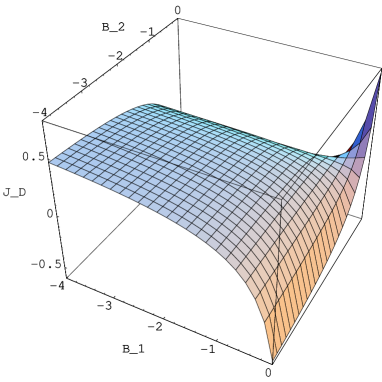
Figure 1: The function $J_{D}(B_{1},B_{2})$ versus $B_{1}$ and $B_{2}$ for $D=4$.

The vacuum energy-momentum tensor on curved background (2) is obtained by the standard transformation law between conformally related problems (see, for instance, [25]) and has the form

$$\langle T_{\nu}^{\mu}\left[g_{\alpha\beta}\right]\rangle_{{\rm ren}}=\langle T_{\nu}^{\mu}\left[g_{\alpha\beta}\right]\rangle_{{\rm ren}}^{(0)}+\langle T_{\nu}^{\mu}\left[g_{\alpha\beta}\right]\rangle_{{\rm ren}}^{(b)}.$$ (17)

Here the first term on the right is the vacuum energy–momentum tensor for the situation without boundaries (gravitational part), and the second one is due to the presence of boundaries. As the quantum field is conformally coupled and the background spacetime is conformally flat the gravitational part of the energy–momentum tensor is completely determined by the trace anomaly and is related to the divergent part of the corresponding effective action by the relation [25]

$$\langle T_{\nu}^{\mu}\left[g_{\alpha\beta}\right]\rangle_{{\rm ren}}^{(0)}=2g^{\mu\sigma}(x)\frac{\delta}{\delta g^{\nu\sigma}(x)}W_{{\rm div}}[g_{\alpha\beta}].$$ (18)

Note that in odd spacetime dimensions the conformal anomaly is absent and the corresponding gravitational part vanishes:

$$\langle T_{\nu}^{\mu}\left[g_{\alpha\beta}\right]\rangle_{{\rm ren}}^{(0)}=0,\quad{\rm for\;even}\;D.$$ (19)

The boundary part in Eq. (17) is related to the corresponding flat spacetime counterpart (12),(16) by the relation [25]

$$\langle T_{\nu}^{\mu}\left[g_{\alpha\beta}\right]\rangle_{{\rm ren}}^{(b)}=\frac{1}{\sqrt{|g|}}\langle\bar{T}_{\nu}^{\mu}\left[\eta_{\alpha\beta}\right]\rangle_{{\rm ren}}.$$ (20)

By taking into account Eq. (12) from here we obtain

$$\langle T_{\nu}^{\mu}\left[g_{\alpha\beta}\right]\rangle_{{\rm ren}}^{(b)}=-\frac{e^{(D+1)\sigma(z)}J_{D}(B_{1},B_{2})}{2^{D}\pi^{D/2}a^{D+1}\Gamma(D/2+1)}{\rm diag}(1,1,\ldots,1,-D),$$ (21)

for $z_{1}<z<z_{2}$, and

$$\langle T_{\nu}^{\mu}\left[g_{\alpha\beta}\right]\rangle_{{\rm ren}}^{(b)}=0,\;{\rm for}\;z<z_{1},z>z_{2}.$$ (22)

In Eq. (21) the constants $B_{j}$ are related to the Robin coefficients in boundary condition (4) by formulae (14),(11) and are functions on $z_{j}$. In particular, for Neumann boundary conditions $B^{(N)}_{j}=2(-1)^{j-1}/[a(D-1)\sigma^{\prime}(z_{j})]$.

The total bulk vacuum energy per unit physical hypersurface on the brane at $z=z_{j}$ is obtained by integrating over the region between the plates

$$E_{j}^{(b)}=e^{D\sigma(z_{j})}\int_{z_{1}}^{z_{2}}\langle T_{0}^{0}\rangle^{(b)}_{{\mathrm{ren}}}e^{-(D+1)\sigma(z)}dz=-\frac{J_{D}(B_{1},B_{2})e^{D\sigma(z_{j})}}{2^{D}\pi^{D/2}\Gamma(D/2+1)a^{D}}.$$ (23)

The resulting vacuum force per unit boundary area acting on the boundary at $z=z_{j}$ is determined by the difference

$$\langle T_{D}^{D}\left[g_{\alpha\beta}\right]\rangle_{{\rm ren}}|_{z=z_{j}+0}-\langle T_{D}^{D}\left[g_{\alpha\beta}\right]\rangle_{{\rm ren}}|_{z=z_{j}-0}.$$ (24)

Now we see that as gravitational part (18) is a continous function on $z$ it does not contribute to the forces acting on the boundaries and the vacuum force per unit surface acting on the boundary at $z=z_{j}$ is determined by the boundary part of the vacuum pressure, $p_{D}=-\langle T_{D}^{D}\left[g_{\alpha\beta}\right]\rangle_{{\rm ren}}^{(b)}$, taken at the point $z=z_{j}$:

$$p_{Dj}(z_{1},z_{2})=-\frac{e^{(D+1)\sigma(z_{j})}J_{D}(B_{1},B_{2})}{2^{D-1}\pi^{D/2}a^{D+1}\Gamma(D/2)}.$$ (25)

This corresponds to the attractive/repulsive force between the plates if $p_{Dj}</>0$. The equilibrium points for the plates correspond to the zero values of Eq. (25): $p_{Dj}=0$. These points are zeros of the function $J_{D}(B_{1},B_{2})$ defined by Eq. (13) and are the same for both plates. Note that at these points the VEV’s of the bulk energy-momentum tensor given by Eq. (21) and the total bulk energy also vanish. The location of these zeros on the quadrant $B_{1,2}\leq 0$ of the plane $(B_{1},B_{2})$ for $D=4$ is plotted in Fig. 2. The function $J_{D}(B_{1},B_{2})$ is positive in the region between the curves (including the point $(0,0)$) and is negative outside of this region. When $B_{1}=0$ the zero for the function $J_{4}(B_{1},B_{2})$ is obtained for $B_{2}\approx-0.459$. In the limit $B_{1}\to\infty$ for the zero one has $B_{2}\approx-0.451$.

Figure 2: The location of zeros for the function $J_{D}(B_{1},B_{2})$ on the quadrant $B_{1,2}\leq 0$ of the plane $(B_{1},B_{2})$ for $D=4$.

3 Casimir densities and vacuum forces on AdS background

As an application of the general formulae from the previous section here we consider the important special case of the AdS_D+1 bulk for which

$$\sigma=\ln(k_{D}z)=k_{D}y,$$ (26)

with $1/k_{D}$ being the AdS curvature radius. Now the expressions for the coefficients $B_{j}$, $j=1,2$ take the form

$$B_{j}=\frac{b_{j}k_{D}z_{j}}{(z_{2}-z_{1})\left[a_{j}+(-1)^{j-1}(D-1)k_{D}b_{j}/2\right]}.$$ (27)

Note that the ratio $z_{2}/z_{1}$ is related to the proper distance between the branes $\Delta y$ by the formula

$$z_{2}/z_{1}=e^{k_{D}\Delta y},\quad\Delta y=y_{2}-y_{1}.$$ (28)

For the boundary induced part of the vacuum energy-momentum tensor one has

$$\langle T_{\nu}^{\mu}\left[g_{\alpha\beta}\right]\rangle_{{\rm ren}}^{(b)}=-\left(\frac{k_{D}z}{z_{2}-z_{1}}\right)^{D+1}\frac{J_{D}(B_{1},B_{2})}{2^{D}\pi^{D/2}\Gamma(D/2+1)}{\rm diag}(1,1,\ldots,1,-D),$$ (29)

where $B_{j}$ are functions on the distance between the branes. The bulk vacuum energy per unit hypersurface on the brane $z=z_{j}$ is obtained from (23):

$$E_{j}^{(b)}=-\left(\frac{k_{D}z_{j}}{z_{2}-z_{1}}\right)^{D}\frac{J_{D}(B_{1},B_{2})}{2^{D}\pi^{D/2}\Gamma(D/2+1)}.$$ (30)

The vacuum forces per unit surface are functions on the proper distance $\Delta y$ and on the ratio $a_{j}/b_{j}$ of the Robin coefficients:

$$p_{Dj}=-\left(\frac{k_{D}z_{j}}{z_{2}-z_{1}}\right)^{D+1}\frac{J_{D}(B_{1},B_{2})}{2^{D-1}\pi^{D/2}\Gamma(D/2)},\quad j=1,2.$$ (31)

In Fig. 3 we have plotted the vacuum forces acting per unit surface of the branes as functions of $k_{D}\Delta y$ for the values of parameters $a_{1}/k_{D}b_{1}=-3$, $a_{2}/k_{D}b_{2}=-1$ and $D=4$. As we see from these graphics there is an equilibrium point at $\Delta y_{0}\approx 0.95/k_{D}$, where the vacuum forces vanish. These forces are repulsive for $\Delta y<\Delta y_{0}$ ($p_{Dj}>0$) and are attractive for $\Delta y>\Delta y_{0}$ ($p_{Dj}<0$). As a result the equilibrium point is stable. Hence, we have an example for the stabilization of the distance between the plates due to the vacuum forces.

Figure 3: The vacuum forces acting per unit surfaces of the branes on the AdS background, $10^{5}p_{D1}/k_{D}^{D+1}$ (left panel) and $10^{2}p_{D2}/k_{D}^{D+1}$ (right panel) for $D=4$ versus $k_{D}\Delta y$.

Now we turn to the brane–world model introduced by Randall and Sundrum [3] and based on the AdS geometry with one extra dimension. The fifth dimension $y$ is compactified on an orbifold, $S^{1}/Z_{2}$ of length $\Delta y$, with $-\Delta y\leq y\leq\Delta y$. The orbifold fixed points at $y=0$ and $y=\Delta y$ are the locations of two 3-branes. For the conformal factor in this model one has $\sigma=k_{D}|y|$. The boundary conditions for the corresponding conformally coupled bulk scalars have the form (6) with Robin coefficients $a_{j}/b_{j}=-c_{j}k_{D}$, where the constants $c_{j}$ are the coefficients in the boundary mass term [6]:

$$m_{\varphi}^{(b)2}=2k_{D}\left[c_{1}\delta(y)+c_{2}\delta(y-\Delta y)\right].$$ (32)

Note that here we consider the general case when the boundary masses are different for different branes. Supersymmetry requires $c_{2}=-c_{1}$. The boundary induced part of the VEV’s for the energy-momentum tensor on the Randall-Sundrum brane-world background are obtained from Eq. (29) with additional factor 1/2. This factor is related to the fact that now in the normalization condition for the eigenfunctions the integration goes over the region $(-\Delta y,\Delta y)$, instead of $(0,\Delta y)$. The expressions for the total energy and vacuum forces remain the same. The coefficients $B_{j}$ in the expression for $J_{D}(B_{1},B_{2})$ are given by the formula (below we will keep $D$ general)

$$B_{j}=-\frac{e^{(j-1)k_{D}\Delta y}}{e^{k_{D}\Delta y}-1}\frac{1}{c_{j}+(-1)^{j}(D-1)/2}.$$ (33)

In the Randall-Sundrum model, the hierarchy problem is solved if $k_{D}\Delta y\approx 37$. For these values of distances between the branes one has $|B_{1}|\ll|B_{2}|$ under the assumption $c_{1}\sim c_{2}$.

Expression (30) takes into account the Casimir energy of the bulk. In general, the total vacuum energy receives additional contribution coming from the vacuum energy located on branes. In the case of general mixed boundary conditions the decomposition of the vacuum energy into surface and volume parts is presented in Ref. [22] for the Minkowski background. The corresponding results for a conformally coupled scalar on the AdS bulk is obtained by a way similar to that described above. For the total vacuum energy per unit hypersurface on the brane $z=z_{j}$ this yields

$$E_{j}^{(b){\mathrm{tot}}}=-\left(\frac{k_{D}z_{j}}{z_{2}-z_{1}}\right)^{D}\frac{2^{-D-1}\pi^{-D/2}}{\Gamma(D/2+1)}{\mathrm{p.v.}}\int_{0}^{\infty}dt\,t^{D}\frac{d}{dt}\ln\left[1-\frac{(B_{1}t+1)(B_{2}t+1)}{(B_{1}t-1)(B_{2}t-1)}e^{-2t}\right].$$ (34)

In addition, the vacuum energy per unit hypersurface on the brane $z=z_{j}$ can contain terms in the form $k_{D}^{D}\sum_{l=1}^{2}\alpha_{l}(z_{j}/z_{l})^{D}$ with constants $\alpha_{1}$ and $\alpha_{2}$ and corresponding to the single brane contributions when the second brane is absent. Adding these terms to the vacuum energy corresponds to finite renormalization of the tension on both branes (see [10, 13] for more detailed discussion).

4 Conclusion

In the present paper we have investigated the Casimir effect for a conformally coupled scalar field confined in the region between two parallel branes on background of the conformally-flat plane symmetric spacetimes. The general case of the mixed boundary conditions is considered. The vacuum expectation values of the energy-momentum tensor are derived from the corresponding flat spacetime results by using the conformal properties of the problem. The purely gravitational part arises due to the trace anomaly and is zero for odd spacetime dimensions. In the region between the branes the boundary induced part for the vacuum energy-momentum tensor is given by formula (21), and the corresponding vacuum forces acting per unit surface of the brane have the form Eq. (25). These forces vanish at the zeros of the function $J_{D}(B_{1},B_{2})$. In the case $B_{1,2}\leq 0$ the subintegrand in Eq. (25) has no real poles and the location of these zeros for $D=4$ is plotted in Fig. 2. Further we consider a special case of the AdS bulk with the brane induced vacuum energy-momentum tensor given by Eq. (21). On a specific example we demonstrate that there are stable equilibrium points, where the vacuum forces vanish and the radion field is stabilized. An application to the Randall-Sundrum brane-world model is discussed. In this model the coefficients in the Robin boundary conditions on branes are related to the boundary mass terms for the scalar field under consideration. In the present paper we have considered the geometry of flat branes. The corresponding results for spherical branes can be obtained by applying the same method of conformal transformation to the corresponding flat spacetime vacuum energy-momentum tensor given in [23] (for the total Casimir energy in the cases of spherical one and two brane configurations see Refs. [12, 14]).

References

- [1] E. Witten, Nucl. Phys. B471, 135 (1996); P. Horava and E. Witten, Nucl. Phys. B460, 506 (1996); T. Banks and M. Dine, Nucl. Phys. B479, 173 (1996).
- [2] N. Arkani-Hamed, S. Dimopoulos, and G. Dvali, Phys. Lett. B429, 263 (1998); Phys. Rev. D59, 086004 (1999); I. Antoniadis, N. Arkani-Hamed, S. Dimopoulos, and G. Dvali, Phys. Lett. B436, 257 (1998).
- [3] L. Randall and R. Sundrum, Phys. Rev. Lett. 83, 3370 (1999).
- [4] M. Gell-Mann and B. Zwiebach, Phys. Lett. B141, 333 (1984); Nucl. Phys. B260, 569 (1985).
- [5] W. D. Goldberger and M. B. Wise, Phys. Rev. Lett. 83, 4922 (1999); Phys. Rev. D60, 107505 (1999); C. Csaki, J. Erlich, T. Hollowood, and Y. Shirman, Nucl. Phys. B581, 309 (2000); K. Maeda and D. Wands, Phys. Rev. D62, 124009 (2000); C. Barcelo and M. Visser, Phys. Rev. D63, 024004 (2001).
- [6] T. Gherghetta and A. Pomarol, Nucl. Phys. B586, 141 (2000).
- [7] P. Kanti, K. A. Olive, and M. Pospelov, Phys. Lett. B481,386 (2000).
- [8] V. Barger, T. Han, T. Li, J. D. Lykken, and D. Marfatia, Phys. Lett. B488, 97 (2000).
- [9] M. Fabinger and P. Horava, Nucl. Phys. B580, 243 (2000).
- [10] J. Garriga, O. Pujolas, and T. Tanaka, Nucl. Phys. B605, 192 (2001).
- [11] S. Nojiri, S. Odintsov, and S. Zerbini, Phys. Rev. D62, 064006 (2000).
- [12] S. Nojiri, S. Odintsov, and S. Zerbini, Class. Quantum Grav. 17, 4855 (2000).
- [13] S. Nojiri and S. Odintsov, Phys. Lett. B484, 119 (2000); S. Nojiri, O. Obregon, and S. Odintsov, Phys. Rev. D62, 104003 (2000); D. J. Toms, Phys. Lett. B484, 149 (2000); W. Goldberger and I. Rothstein, Phys. Lett. B491, 339 (2000); S. Nojiri and S. Odintsov, JHEP 0007, 049 (2000); I. Brevik, K. A. Milton, S. Nojiri, and S. D. Odintsov, Nucl. Phys. B599, 305 (2001); A. Flachi and D. J. Toms, Nucl. Phys. B599, 305 (2001); R. Hofmann, P. Kanti, and M. Pospelov, Phys. Rev. D63, 124020 (2001).
- [14] W. Naylor and M. Sasaki, Phys. Lett. B542, 289 (2002).
- [15] M. R. Setare and R. Mansouri, Class. Quantum Grav. 18, 2695 (2001).
- [16] N. Kaloper, J. March-Russel, G. D. Starkman, and M. Trodden, Phys. Rev. Lett. 85, 928 (2000).
- [17] M. Trodden, Diluting gravity with compact hyperboloids, hep-th/0010032.
- [18] G. D. Starkman, D. Stojkovic, and M. Trodden, Phys. Rev. Lett. 87, 231303 (2001).
- [19] G. D. Starkman, D. Stojkovic, and M. Trodden, Phys. Rev. D63, 103511 (2001).
- [20] S. Nasri, P. J. Silva, G. D. Starkman, and M. Trodden, Radion stabilization in compact hyperbolic extra dimensions, hep-th/0201063.
- [21] M. R. Setare and A. A. Saharian, Int. J. Mod. Phys. A16, 1463 (2001).
- [22] A. Romeo and A. A. Saharian, J. Phys. A: Math. Gen., 35, 1297 (2002).
- [23] A. A. Saharian, Phys. Rev. D63, 125007 (2001).
- [24] A. Romeo and A. A. Saharian, Phys. Rev. D63, 105019 (2001).
- [25] N. D. Birrel and P. C. W. Davies, Quantum Fields in Curved Space (Cambridge: Cambridge University Press, 1982).