BA-TH/02-437
CERN-TH/2002-104
hep-th/0207130
The Pre-Big Bang Scenario
in String Cosmology
M. Gasperini1 and G. Veneziano2
1Dipartimento di Fisica , Università di Bari,
Via G. Amendola 173, 70126 Bari, Italy
and
Istituto Nazionale di Fisica Nucleare, Sezione di Bari
Via G. Amendola 173, 70126 Bari, Italy
E-mail: maurizio.gasperini@ba.infn.it
2Theory Division, CERN,
CH-1211 Geneva 23, Switzerland
E-mail: gabriele.veneziano@cern.ch
We review physical motivations, phenomenological consequences, and open problems of the so-called pre-big bang scenario in superstring cosmology.
1 Introduction
During the past thirty years, mainly thanks to accelerator experiments of higher and higher energy and precision, the standard model of particle physics has established itself as the uncontested winner in the race for a consistent description of electroweak and strong interaction phenomena at distances above cm or so. There are, nonetheless, good reasons (in particular the increasing evidence for non-vanishing neutrino masses [389, 569, 570]) to believe that the standard model is not the end of the story. The surprising validity of this model at energies below GeV, as well as the (in)famous Higgs mass fine-tuning problem, suggest some supersymmetric extension of the standard model (for a review see [502]) as the most likely improved description of non-gravitational phenomena over a few more decades in the ladder of scales. It is however quite likely that other questions that are left unanswered by the standard model, such as the peculiarities of fermionic masses and mixings, the family pattern, C, P, CP, B violation, etc., will only find their answers at –or around– the much higher energies at which all gauge interactions appear to unify [22]. This energy scale appears to be embarrassingly close (on a logarithmic scale) to the so-called Planck mass, GeV, the scale at which gravity becomes strong and needs to be quantized.
The situation with gravitational phenomena is completely different. Even the good old Newton law is known to be valid only down to the mm scale [381], so that much interest has been devoted to the possibility of large modifications of gravity below that distance, either from new forces mediated by light scalars such as the dilaton of string theory [578], or from the existence of large extra dimensions felt exclusively by gravity [36, 531]. General relativity is well tested at large scales; nevertheless; present evidence for a (small) vacuum energy density [536, 517] suggests that, even on cosmologically large distances, the strict Einstein theory might turn out to be inadequate. Evidently, the construction of a standard model for gravity and cosmology lags much behind its particle physics counterpart.
The hot big bang model (see for instance [619]), originally thought of as another great success of general relativity, was later discovered to suffer from huge fine-tuning problems. Some of these conceptual problems are solved by the standard inflationary paradigm (see [442, 421] for a review), yet inflation remains a generic idea in search of a theory that will embody it naturally. Furthermore, the classical theory of inflation does not really address the problem of how the initial conditions needed for a successful inflation came about. The answer to this question is certainly related to even more fundamental issues, such as: How did it all start? What caused the big bang? Has there been a singularity at ? Unfortunately, these questions lie deeply inside the short-distance, high-curvature regime of gravity where quantum corrections cannot be neglected. Attempts at answering these questions using quantum cosmology based on Einstein’s theory has resulted in a lot of heated discussions [444, 593], with no firm conclusions.
It is very likely that both a standard model for gravity and cosmology and a full understanding of the standard model of particle physics will require our understanding of physics down to the shortest scale, the Planck length cm. Until the Green–Schwarz revolution of 1984 [347], the above conclusion would have meant postponing indefinitely those kinds of questions. Since then, however, particle theorists have studied and developed superstring theory (see [525] for a recent review, as well as [348] for a non-specialized introduction), which appears to represent a consistent framework not only for addressing (and possibly answering) those questions, but even for unifying our understanding of gravitational and non-gravitational phenomena, and therefore for relating the two classes of questions.
The so-called “pre-big bang” scenario described in this report has to be seen in the above perspective as a possible example, even just as a toy model, of what cosmology can look like if we assume that the sought for standard model of gravity and cosmology is based on (some particular version of) superstring theory. Although most string theorists would certainly agree on the importance of studying the cosmological consequences of string theory, it is a priori far from obvious that the “state of the art” in this field can provide an unambiguous answer to this question. Indeed, most of our understanding of superstring theory is still based on perturbative expansions, while most of the recent progress in non-perturbative string theory has been achieved in the context of “vacua” (i.e. classical solutions to the field equations) that respect a large number of supersymmetries [525]. By contrast, our understanding of string theory at large curvatures and couplings, especially in the absence of supersymmetry, is still largely incomplete. A cosmological background, and a fortiori one that evolves rapidly in time, breaks (albeit spontaneously) supersymmetry. This is why the Planckian regime of cosmology appears to be intractable for the time being.
It is very fortunate, in this respect, that in the pre-big bang scenario the Universe is supposed to emerge from a highly perturbative initial state preceding the big bang. Therefore, early enough before (and late enough after) the big bang, we may presume to know the effective theory to be solved. The difficult part to be dealt with non-perturbatively remains the transition from the pre- to the post-big bang regime, through a high-curvature (and/or possibly a large-coupling) phase. Thus, from a more phenomenological standpoint, the relevant question becomes: Are the predictions of the pre-big bang scenario robust with respect to the details of the non-perturbative phase?
It is difficult of course to give a clear-cut answer to this question, but an analogy with QCD and the physics of strong interactions may be helpful. Because of asymptotic freedom, QCD can be treated perturbatively at short distance (high momentum transfers). However, even “hard” processes such as are not fully within perturbative control. Some soft non-perturbative physics always gets mixed in at some level, e.g. when partons eventually turn into hadrons. The reason why certain sufficiently inclusive quantities are believed to be calculable is that large- and short-distance physics “decouple”, so that, for instance, the hadronization process does not affect certain “infrared-safe” quantities, computed at the quark–gluon level.
In the case of string cosmology the situation should be similar, although somehow reversed [601]. For gravity, in fact, the large-distance, small-curvature regime is easy to deal with, while the short-distance, high-curvature is hard. Yet, we shall argue that some consequences of string cosmology, those concerning length scales that were very large with respect to the string scale (or the horizon) in the high-curvature regime, should not be affected (other than by a trivial kinematical redshift) by the details of the pre- to post-big bang transition. The above reasoning does not imply, of course, that string theorists should not address the hard, non-perturbative questions now. On the contrary, the “easy” part of the game will provide precious information about what the relevant hard questions are, and on how to formulate them.
Finally, possible reservations on a “top–down” string cosmology approach may naturally arise from a cosmology community accustomed to a data-driven, “bottom–up” approach. We do believe ourselves that a good model of cosmology is unlikely to emerge from theoretical considerations alone. Input from the data will be essential in the selection among various theoretical alternatives. We also believe, however, that a balanced combination of theoretical and experimental imput should be the best guarantee for an eventual success.
Insisting on the soundness of the underlying theory (e.g. on its renormalizability) was indeed essential in the progressive construction of the standard model, just as were the quantity and the quality of experimental data. Cosmology today resembles the particle physics of the sixties: there is no shortage of data, and these are becoming more and more precise but also more and more challenging while, theoretically, we are still playing with very phenomenological (even if undoubtedly successful) models, lacking a clear connection to other branches of fundamental physics, and therefore remaining largely unconstrained.
1.1 Coping with a beginning of time
Both the standard Friedmann–Robertson–Walker (FRW) cosmological scenario [619] and the standard inflationary scenario [361, 421, 442] assume that time had a beginning. Many of the problems with the former model simply stem from the fact that, at the start of the classical era, so little time had elapsed since the beginning. Indeed, in the FRW framework, the proper size of the (now observable) Universe was about cm across at the start of the classical era, say at a time of the order of a few Planck times, s. This is of course a very tiny Universe with respect to its present size (), yet it is huge with respect to the horizon (the distance travelled by light) at that time, cm.
In other words, a few Planck times after the big bang, our observable Universe consisted of about Planckian-size, causally disconnected regions. Simply not enough time had elapsed since the beginning for the Universe to become homogeneous (e.g. to thermalize) over its entire size. Furthermore, soon after , the Universe must have been characterized by a huge hierarchy between its Hubble radius, on the one hand, and its spatial-curvature radius, on the other. The relative factor of (at least) appears as an incredible amount of fine-tuning on the initial state of the Universe, corresponding to a huge asymmetry between space and time derivatives, or, in more abstract terms, between intrinsic and extrinsic curvature. Was this asymmetry really there? And, if so, can it be explained in any, more natural way?
The conventional answer to the difficulties of the standard scenario is to wash out inhomogeneities and spatial curvature by introducing, in the history of the Universe, a long period of accelerated expansion, called inflation [361, 421, 442]. It has been pointed out, however, that standard inflation cannot be “past-eternal” [95] (and cannot avoid the initial singularity [613, 96]), so that the question of what preceded inflation is very relevant. Insisting on the assumption that the Universe (and time itself) started at the big bang leaves only the possibility of having post-big bang inflation mend an insufficiently smooth and flat Universe arising from the big bang.
Unfortunately, that solution has its own problems, for instance those of fine-tuned initial conditions for the inflaton field and its potential. A consistent quantum cosmology approach giving birth to a Universe in the “right” initial state is still much under debate [371, 610, 441, 634, 542]. Furthermore, the inflaton is introduced ad hoc and inflation is not part of a grander theory of elementary particles and fundamental interactions such as superstring theory. In spite of its possible importance, and of repeated motivated attempts [237, 462, 90], a conventional realization of an inflationary phase in a string theory context is in fact problematic [142], in particular because the dilaton –the fundamental string theory scalar– cannot be (at least trivially) identified with the inflaton –the fundamental scalar of the standard inflationary scenario [126].
Here we shall argue that, instead, superstring theory gives strong hints in favour of a totally different approach to solving the problems of the standard cosmological scenario. This new possibility arises if we assume that, in string theory, the big bang singularity is fictitious and that it makes therefore sense to “continue” time to the past of the big bang itself.
1.2 Inflation before the big bang
If the history of the Universe can be continued backward in time past the big bang, new possibilities arise for a causal evolution to have produced a big bang with the desired characteristics. The actual pre-big bang scenario presented in this report is just one possible realization of the above general idea. Since, as we shall see, it is easy to generate a phase of pre-big bang inflation driven by the kinetic energy of the dilaton (somewhat in analogy with kinetic-inflation ideas [430]), we will discuss, as the simplest possibility, a minimal cosmological scenario, which avoids making use of standard (i.e. potential-energy-driven) post-big bang inflation.
This does not, though, that pre- and post-big bang inflation are mutually exclusive or incompatible. Should near-future high-precision experiments definitely indicate that an inflation that is exclusively of the pre-big bang type is disfavoured with respect to conventional, post-big bang, “slow-roll” inflation, one should ask whether a pre-big bang phase can naturally lead to “initial” conditions suitable for igniting an inflationary epoch of the slow-roll type, rather than a standard, non-inflationary, FRW cosmology.
One model-independent feature of pre-big bang cosmology is clear: by its very definition, the pre-big bang phase should be an evolution towards –rather than away from– a high-curvature regime. As we shall see in Section 2, this is precisely what the symmetries of the string cosmology equations suggest, an unconventional realization of the inflationary scenario, in which the phase of accelerated cosmological evolution occurs while the Universe is approaching –rather than getting away from– the high-curvature, Planckian regime.
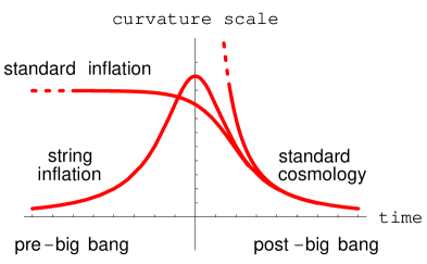
The main difference between the string cosmology and the standard inflationary scenarios can therefore be underlined through the opposite behaviour of the curvature scale as a function of time, as shown in Fig. 1.1. As we go backward in time, instead of a monotonic growth (predicted by the standard scenario), or of a “de-Sitter-like” phase of nearly constant curvature (as in the conventional inflationary picture), the curvature grows, reaches a maximum controlled by the string scale , and then starts decreasing towards an asymptotically flat state, the string perturbative vacuum. The big bang singularity is regularized by a “stringy” phase of high but finite curvature, occurring at the end of the initial inflationary evolution.
We should warn the reader, from the very beginning of this review, that this scenario is far from being complete and understood in all of its aspects, and that many important problems are to be solved still. Nevertheless, the results obtained up to now have been encouraging, in the sense that it now seems possible to formulate models for the pre-big bang evolution of our Universe that fit consistently in a string theory context, and which are compatible with various phenomenological and theoretical bounds. Not only: the parameter space of such models seems to be accessible to direct observations in a relativiely near future and, at present, it is already indirectly constrained by various astrophysical, cosmological, and particle physics data.
To close this subsection we should mention, as a historical note, that the idea of a phase of growing curvature preceding that of standard decelerated expansion, is neither new in cosmology, nor peculiar to string theory. Indeed, if the growth of the curvature corresponds to a contraction, it is reminiscent of Tolman’s cyclic Universe [579], in which the birth of our present Universe is preceded by a phase of gravitational collapse (see also [226, 93, 504]). Also, and more conventionally, the growth of the curvature may be implemented as a phase of Kaluza–Klein superinflation [564, 2, 420], in which the accelerated expansion of our three-dimensional space is sustained by the contraction of the internal dimensions and/or by some exotic source, with the appropriate equation of state (in particular, strings [316] and extended objects).
In the context of general relativity, however, the problem is how to avoid the curvature singularity appearing at the end of the phase of growing curvature. This is in general impossible, for both contraction and superinflationary expansion, unless one accepts rather drastic modifications of the classical gravitational theory. In the contracting case, for instance, the damping of the curvature and a smooth transition to the phase of decreasing curvature can be arranged through the introduction of a non-minimal and gauge-non-invariant coupling of gravity to a cosmic vector [505] or scalar [556, 57] field, with a (phenomenological) modification of the equation of state in the Planckian curvature regime [541, 622], or with the use of a non-metric, Weyl-integrable connection [504]. In the case of superinflation, a smooth transition can be arranged through a breaking of the local Lorentz symmetry of general relativity [267, 282], a geometric contribution of the spin of the fermionic sources [268], or the embedding of the space-time geometry into a more fundamental quantum phase-space dynamics [137, 270]. In the more exotic context of topological transitions, a smooth evolution from contraction to expansion, through a state of minimal size, is also obtained with the adiabatic compression and the dimensional transmutation of the de Sitter vacuum [317].
In the context of string theory, on the contrary, the growth of the curvature is naturally associated to the growth of the dilaton and of the coupling constants (see for instance Section 2). This effect, on the one hand, sustains the phase of superinflationary expansion, with no need of matter sources or extra dimensions. On the other hand, it necessarily leads the Universe to a regime in which not only the curvature but also the couplings become strong, so that typical “stringy” effects become important and are expected to smooth out the curvature singularity. This means that there is no need to look for more or less ad hoc modifications of the theory, as string theory itself is expected to provide the appropriate tools for a complete and self-consistent cosmological scenario.
1.3 Pre-big bang inflation and conformal frames
While postponing to the next section the issue of physical motivations, it is important to classify the various inflationary possibilities just from their kinematical properties. To be more precise, let us consider the so-called flatness problem (the arguments are similar, and the conclusions the same, for the horizon problem mentioned in Subsection 1.1). We shall assume, on the basis of the approximate isotropy observed at large scale, that our present cosmological phase can be correctly described by the ordinary Einstein–Friedmann equations. In that case, the gravitational part of the equations contains two contributions from the metric: , coming from the spatial (or intrinsic) curvature, and , coming from the gravitational kinetic energy (or extrinsic curvature). Present observations imply that the spatial curvature term, if not negligible, is at least non-dominant, i.e.
| (1.1) |
On the other hand, during a phase of standard, decelerated expansion, the ratio grows with time. Indeed, if ,
| (1.2) |
so that is growing both in the matter-dominated () and in the radiation-dominated () era. Thus, as we go back in time, becomes smaller and smaller. If, for instance, we wish to impose initial conditions at the Planck scale, we must require a fine-tuning suppressing by orders of magnitude the spatial curvature term with respect to the other terms of the cosmological equations. Even if initial conditions are given at a lower scale (say the GUT scale) the amount of fine-tuning is still nearly as bad.
This problem can be solved by introducing an early phase during which the value of , initially of order , decreases so much in time that its subsequent growth during FRW evolution keeps it still below today. It is evident that, on pure kinematic grounds, this requirement can be implemented in two classes of backgrounds.
-
(I)
: . This class of background corresponds to what is conventionally called “power inflation” [448], describing accelerated expansion and decreasing curvature scale, , , . It contains, as the limiting case (), exponential de Sitter inflation, , , describing accelerated expansion with constant curvature.
- (II)
In the first class of backgrounds, corresponding to post-big bang inflation, the Universe is driven away from the singularity/high-curvature regime, while in the second class inflation drives the Universe towards it, with the typical pre-big bang behaviour illustrated in Fig. 1.1. We may thus immediately note a very important “phenomenological” difference between post- and pre-big bang inflation. In the former case the Planck era lies very far in the past, and its physics remains screened from present observations, since the scales that probed Planckian physics are still far from re-entering. By contrast, in the pre-big bang case, the Planck/string regimes are closer to us (assuming that no or little inflation occurs after the big bang itself). Scales that probe Planckian physics are now the first to re-enter, and to leave an imprint for our observations (see, for instance, the case of a stochastic background of relic gravitational waves, discussed in Section 5).
The inflationary character of Class IIa backgrounds is well known, and recognized since the earlier studies of the inflationary scenario [448]. The inflationary character of Class IIb is more unconventional –a sort of “inflation without inflation” [274], if we insist on looking at inflation as accelerated expansion– and was first pointed out only much later [321]. It is amusing to observe that, in the pre-big bang scenario, both subclasses IIa and IIb occur. However, as discussed in detail in Subsection 2.5, they do not correspond to different models of pre-big bang inflation, but simply to different kinematical representations of the same scenario in two different conformal frames.
In order to illustrate this point, which is important also for our subsequent arguments, we shall proceed in two steps. First we will show that, through a field redefinition , , it is always possible to move from the string frame (S-frame), in which the lowest order gravidilaton effective action takes the form
| (1.3) |
to the Einstein frame (E-frame), in which the dilaton is minimally coupled to the metric and has a canonical kinetic term:
| (1.4) |
(see Subsection 1.4 for notations and conventions). Secondly, we will show that, by applying such a redefinition, a superinflationary solution obtained in the S-frame becomes an accelerated contraction in the E-frame, and vice versa.
We shall consider, for simplicity, an isotropic, spatially flat background with spatial dimensions, and set:
| (1.5) |
where is to be fixed by an arbitrary gauge choice. For this background the S-frame action (1.3) becomes, modulo a total derivative,
| (1.6) |
where, as expected, has no kinetic term and plays the role of a Lagrange multiplier. In the E-frame the variables are , and the action(1.4), after integration by parts, takes the canonical form
| (1.7) |
A quick comparison with Eq. (1.6) finally leads to the field redefinition (not a coordinate transformation!) connecting the Einstein and String frames:
| (1.8) |
Consider now an isotropic, -dimensional vacuum solution of the action (1.6), describing a superinflationary, pre-big bang expansion driven by the dilaton (see Section 2) [490, 600], of Class IIa, with :
| (1.9) |
and look for the corresponding E-frame solution. Since the above solution is valid in the synchronous gauge, , we can choose, for instance, the synchronous gauge also in the E-frame, and fix by the condition:
| (1.10) |
which defines the E-frame cosmic time as:
| (1.11) |
After integration
| (1.12) |
the transformed solution takes the form:
| (1.13) |
It can easily be checked that this solution describes accelerated contraction of Class IIb, with growing dilaton and growing curvature scale:
| (1.14) |
The same result applies if we transform other isotropic solutions from the String to the Einstein frame, for instance the superinflationary solutions with perfect fluid sources [321], presented in Section 2.
To conclude this section, and for later use, let us stress that the main dynamical difference between post-big bang inflation, Class I metrics, and pre-big bang inflation, Class II metrics, can also be conveniently illustrated in terms of the proper size of the event horizon, relative to a given comoving observer.
Consider in fact the proper distance of the event horizon from a comoving observer, at rest in an isotropic, conformally flat background [537]:
| (1.15) |
Here is the maximal allowed extension, towards the future, of the cosmic time coordinate for the given background manifold. The above integral converges for all the above classes of accelerated (expanding or contracting) scale factors. In the case of Class I metrics we have, in particular,
| (1.16) |
for power-law inflation (), and
| (1.17) |
for de Sitter inflation. For Class II metrics () we have instead
| (1.18) |
In all cases the proper size evolves in time like the so-called Hubble horizon (i.e. the inverse of the modulus of the Hubble parameter), and then like the inverse of the curvature scale. The size of the horizon is thus constant or growing in standard inflation (Class I), decreasing in pre-big bang inflation (Class II), both in the S-frame and in the E-frame.
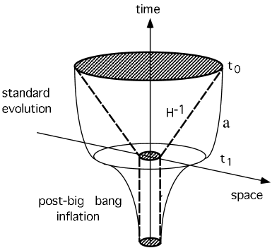
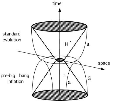
Such an important difference is clearly illustrated in Figs. 1.2 and 1.3, where the dashed lines represent the evolution of the horizon and the solid curves the evolution of the scale factor. The shaded area at time represents the portion of Universe inside our present Hubble radius. As we go back in time, according to the standard scenario, the horizon shrinks linearly (); however, the decrease of the scale factor is slower, so that, at the beginning of the phase of standard evolution (), we end up with a causal horizon much smaller than the portion of Universe that we presently observe. This is the “horizon problem” already mentioned at the beginning of this section.
In Fig. 1.2 the phase of standard evolution is preceded in time by a phase of standard, post-big bang (in particular de Sitter) inflation. Going back in time, for , the scale factor keeps shrinking, and our portion of Universe “re-enters” the Hubble radius during a phase of constant (or slightly growing in time) horizon.
In Fig. 1.3 the standard evolution is preceded in time by a phase of pre-big bang inflation, with growing curvature. The Universe “re-enters” the Hubble radius during a phase of shrinking horizon. To emphasize the difference, we have plotted the evolution of the scale factor both as expanding in the S-frame, , and as contracting in the E-frame, . Unlike in post-big bang inflation, the proper size of the initial portion of the Universe may be very large in strings (or Planck) units, but not larger than the initial horizon itself [287], as emphasized in the picture, and as will be discussed in a more quantitative way in Section 2.4. The initial horizon is large because the initial curvature scale is small (in string cosmology, in particular, ).
This is a basic consequence of the choice of the initial state; in the context of the string cosmology scenario, this approaches the flat, cold and empty string perturbative vacuum, (see the discussion of Section 3). This initial state has to be contrasted with the extremely curved, hot and dense initial state of the standard scenario, characterizing a Universe that starts inflating at (or soon after) the Planck scale, (see also [289] for a more detailed comparison and discussion of pre-big bang versus post-big bang inflation).
1.4 Outline, notations and conventions
We give here a general overlook at the material presented in the various sections of this report. Furthermore, each section will begin with an outline of the content of each of its subsections, and will try to be as self-contained as possible, in order to help the reader interested only in some particular aspects of this field.
In Section 2, after a very quick reminder of some relevant properties of superstring theory, we review the string-theoretic motivations behind the pre-big bang scenario, and outline the main ideas. In Section 3, after formulating on the basis of the previous discussion a postulate of “ asymptotic past triviality”, we discuss, within that framework, the problem of initial conditions and fine-tuning.
As a preliminary to the discussion of the observational consequences of the pre-big bang scenario, Section 4 presents some general results on the evolution of quantum fluctuations. Section 5 will deal with the specific case of tensor (metric) perturbations and Section 6 with scalar (dilatonic) ones, while Section 7 will consider gauge (in particular electromagnetic) and axionic perturbations, and their possible physical relevance to galactic magnetic fields and large scale structure, respectively.
The last part of this report is devoted to various open problems, in particular to the possibility of a smooth transition from the pre- to the post-big bang regime, the so-called “exit problem” (Section 8). Several lines of approach to (and partial solutions of) this problem are presented, including a discussion of heat and entropy production in pre-big bang cosmology. A possible minisuperspace approach to the quantum regime will be illustrated in Section 9. Finally, Section 10 contains the discussion of a possible dilatonic interpretation of the quintessence, a short presentation of other open problems, and an outlook.
For further study of string cosmology and of the pre-big bang scenario, we also refer the interested reader to other review papers [438, 289, 64, 245, 103], as well as to two recent introductory lectures [290, 606]. A regularly updated collection of selected papers on the pre-big bang scenario is also available at [266].
We finally report here our conventions for the metric and the curvature tensor, together with the definitions of some variables frequently used in the paper.
We shall always use natural units . Unless otherwise stated, the metric signature is fixed by ; the Riemann and Ricci tensors are defined by
| (1.19) |
In particular, for a Bianchi-I-type metric, and in the synchronous gauge,
| (1.20) |
our conventions lead to
| (1.21) |
where . In a space-time manifold, Greek indices run from to , while Latin indices run from to .
The duality invariant dilatonic variable, the “shifted dilaton” , is referred to a -dimensional spatial section of finite volume, , and is defined by
| (1.22) |
In a Bianchi-I-type metric background, in particular, we shall absorb into the constant shift (required to secure the scalar behaviour of under coordinate reparametrizations), and we shall set
| (1.23) |
Finally, is the fundamental length scale of string theory, related to the string mass and to the string tension (the mass per unit length) by
| (1.24) |
At the tree level (i.e. at lowest order) in the string coupling , the string length is related to the Planck length , and to the gravitational constant in dimensions, by
| (1.25) |
In , in particular, the relation between the string and the Planck mass reads
| (1.26) |
We shall often work in units such that , i.e. , in which parametrizes, in the String frame, the (dimensionless) strength of the gravitational coupling.
2 String theory motivations
A very important concept in string theory, as well as in field theory, is that of moduli space, the space of vacua. In field theory, and in the absence of gravity, the coordinates of moduli space label the possible ground states of the theory. It is very important to immediately distinguish classical moduli space from its exact, quantum counterpart. The two are generally different, since a classical-level ground state can fail to be a true ground state when perturbative or non-perturbative quantum corrections are added (consider for instance dynamical symmetry breaking à la Coleman–Weinberg, or the double-well potential in quantum mechanics).
When gravity is added to the picture (and this is always the case in s tring theory) the concept of a lowest-energy state becomes less well defined, since total energy is always zero in a general-covariant theory. It is therefore better, in string theory, to extend the definition of moduli space to include all string backgrounds that allow a consistent string propagation, i.e. those consistent with world-sheet conformal invariance [347]. Such backgrounds correspond to the vanishing of the two-dimensional -model -functions [446] and, at the same time, they can also be shown to satisfy the field equations of an effective action living in ordinary space-time. The most famous example of a consistent background is, for superstrings, Minkowski space-time with trivial (i.e. constant) dilaton and antisymmetric tensor potentials. Unfortunately, even if quantum (i.e. string-loop) corrections are neglected, our knowledge of moduli space is very limited. Basically, apart from a handful of exact conformal field theories, such as the Wess–Zumino–Witten models, only low-energy solutions (i.e. classical solutions of the effective low-energy field theory) are known.
The known solutions are, at the same time, too many and too few. They are too many because they typically leave the vacuum expectation values of a few scalar fields completely undetermined. Such fields correspond to gravitationally coupled massless scalar particles that mediate dangerous long-range forces, badly violating the well-tested equivalence principle. The way out of this problem is clear: these flat directions should be lifted by quantum corrections, typically (in the supersymmetric case) at the non-perturbative level. The known solutions are also too few, because some of them, which we would like to see appearing, are missing: notably those describing gravitational collapse or cosmological backgrounds, which evolve as a function of time from a regime of low curvature and/or coupling to one of high curvature and/or coupling (and vice versa). These solutions are very hard to analyse for two reasons: first, because time evolution spontaneously breaks supersymmetry, rendering the solutions unstable to radiative corrections; secondly, because the solutions go out of theoretical control, as they enter the non-perturbative regime.
For the purpose of this section, the important property of superstring’s moduli space is that it exhibits duality symmetries. Generically, this means that points in moduli space that seem to describe different theories actually describe the same theory (up to some irrelevant relabelling of the fields). Let us illustrate this in the simplest example of -duality (for a review see, for instance, [341]).
Consider a theory of closed strings moving in a space endowed with some compact dimensions, say, for the sake of simplicity, with one extra dimension having the topology of a circle. Let us denote by the radius of this circle. In point-particle theory, momentum along the compact dimension is quantized, in units of . This is also true in string theory, as far as the motion of the string’s centre of mass (a non-oscillatory “zero mode”) is concerned. However, for closed strings moving on a compact space, like our circle, there is a second zero mode: the string can simply wind around the circle an integer number of times. By doing so it acquires winding energy, which is quantized in units of , if is the string tension.
Something remarkable does happen if we replace by . A point particle would certainly notice the difference between and (unless ), since the new momenta will be different from the old ones. A closed string, instead, does not feel the change of since the role of the momenta in the original theory will mow be played by the winding modes, and vice versa. This symmetry of closed string theory has been called -duality and is believed to be exact, at least to all orders of perturbation theory, provided a suitable transformation of the dilaton accompanies the one on the radius (it also has interesting extensions to discrete groups of the type [341]). It is important to stress, in our context, that -duality actually implies that there is a physical lower limit to the dimensions of a compact space, controlled by the string length itself.
When applied to open strings, -duality leads to the concept of Dirichlet strings, or -strings. In other words, while closed strings are self-dual, open strings with Neumann boundary conditions are dual to open strings with Dirichlet boundary conditions, and vice versa. These developments [524] have led to the study of -branes, the manifolds on which the end-points of open -strings are confined; they play a major role in establishing the basic unity of all five known types of -dimensional superstring theories (Type I, Type IIA, Type IIB, HETSO(32), HETE8) as different limits of a single, more fundamental “M-theory” [627].
In order to briefly illustrate this point we start recalling that all superstring theories are actually defined through a double perturbative expansion in two dimensionless parameters: the first, the string coupling expansion, can be seen as the analogue of the loop expansion in quantum field theory, except that the coupling constant gets promoted to a scalar field, the dilaton. Consequently, the range of validity of the loop expansion depends on the value of the dilaton, and can break down in certain regions of space-time if the dilaton is not constant. The second expansion, which has no quantum field theory analogue, is an expansion in derivatives, the dimensionless parameter being , with the fundamental length scale of string theory (see Subsection 2.1). Obviously, the validity of this second expansion breaks down when curvature or field space-time derivatives become of order in string-length units.
One of the most amazing recent developments in string theory [627] is the recognition that the above five theories, rather than forming isolated islands in moduli space, are connected to one another via a web of duality transformations. In the huge moduli space, they represent “corners” where the above-mentioned perturbative expansions are, qualitatively at least, correct. A sixth corner actually should be added, corresponding to -dimensional supergravity [580]. The mysterious theory approaching these six known theories in appropriate limits was given the name of M-theory. It might seem curious, at first sight, that one is able to flow continuously from to dimensions, within a single theory. The puzzle was solved after it was realized that the supergravity theory has no dilaton, hence no free coupling. In other words, the dilaton of the five -dimensional superstring theories becomes (at large coupling) an extra dimension of space [627, 377]. At weak coupling, this extra dimension is so small that one may safely describe physics in dimensions.
In spite of the beauty of all this, the previous discussion shows that the moduli-space diagram connecting the five superstring theories can be quite misleading. Since each point in the diagram is supposed to represent a possible solution of the -function constraints, and the diagram itself is supposed to show how apparently different theories are actually connected by moving in coupling constant (or other moduli-) space, it necessarily includes the flat directions we have been arguing against. At the same time, cosmological solutions of the above-mentioned type, i.e. evolving in different regions of coupling constant/curvature, cannot be “localized” in the diagram. A single cosmology, for instance, may indeed correspond to an initial Universe, well described by heterotic string theory, ending in another Universe better described by perturbative Type I theory. Yet, such a cosmological solution should be only a point, not a curve, in moduli space. As we shall argue below, thanks to some gravitational instability, solutions of the above type are rather the rule than the exception.
It seems appropriate, at this point, to comment on the fact that modern research in string/M-theory looks to be strongly biased towards analysing supersymmetric vacua, or at least solutions that preserve a large number of supersymmetries [525]. While the mathematical motivation for that is quite obvious, and physically interesting results can be rigorously derived in special cases (concerning, for instance, BPS states and black holes), it is quite clear that cosmology, especially inflationary or rapidly evolving solutions, requires extensive breaking of supersymmetries. Given their phenomenological importance, we think that more effort should be devoted to developing new techniques dealing with non-supersymmetric solutions and, in particular, with their high-curvature and/or large-coupling regimes.
In this section we will emphasize the role of the duality symmetry for the pre-big bang scenario, starting from the short- and large-distance properties of string theory (Subsection 2.1), and from the related invariance of the classical cosmological equations under a large group of non-compact transformations (Subsections 2.2, 2.3). We will discuss the inflationary aspects of families of solutions related by such groups of transformations in Subsection 2.4, and will end up with a discussion of the relative merits of the so-called Einstein and String frames (in Subsection 2.5), in spite of their ultimate equivalence.
2.1 Short- and large-distance motivations
Since the classical (Nambu–Goto) action of a string is proportional to the area of the space-time surface it sweeps, its quantization requires the introduction of a fundamental “quantum” of length , through the rlation:
| (2.1) |
As discussed in [598, 599], the appearance of this length in string theory is so much tied to quantum mechanics that, after introducing , we are actually dispensed from introducing itself, provided we use the natural units of energy of string theory, i.e. provided we replace by , the classical length of a string of energy . For instance, the Regge trajectory relation between angular momentum and mass, ( throughout), is rewritten in string units as , where has neatly disappeared.
One of the most celebrated virtues of string theory is its soft behaviour at short distances. This property, which is deeply related to the extended nature of fundamental particles in the theory, makes gravity and gauge interactions not just renormalizable, but finite, at least order by order in the loop expansion [525]. At the same time, the presence of an effective short-distance cut-off in loop diagrams should have a counterpart in a modification of the theory, when the external momenta of the diagram approach the cut-off itself.
An analogy with the standard electroweak theory may be of order here: the Glashow–Weinberg–Salam model makes Fermi’s model softer at short distances, turning a non-renormalizable effective theory into a fully-fledged renormalizable gauge theory. At the same time, the naive predictions of Fermi’s model of electroweak interactions become largely modified when the -mass region is approached. Note that this mass scale, and not , is where new physics comes into play.
In string theory, something similar is expected to occur, this time in the gravitational sector, where Einstein’s effective theory should be recovered at low energy, as soon as the string scale (and not ) is reached. At present, there are not so many available tests of this idea: one comes from the study of trans-Planckian energy collisions in string theory [23, 24]. When one prepares the initial state in such a way as to expect the formation of tiny black holes, having radius (or curvature) respectively smaller (or larger) than the fundamental scale of string theory, one finds that such objects are simply not formed. Arguments based on entropy considerations [99] also suggest that the late stage of black hole evaporation ends, in string theory, into a normal non-collapsed string state of radius equal to the string length, rather than into a singularity. Finally, we recall the arguments from -duality for a minimal compactification scale, given at the beginning of this section.
This considerable amount of circumstantial evidence leads to the conclusion that plays, in string theory, the role of a minimal observable length, i.e. of an ultraviolet cut-off. Physical quantities are expected to be bounded (in natural units) by the appropriate powers of , e.g. the curvature scale , the temperature , the compactification radius , and so on. It follows, in particular, that space-time singularities are expected to be avoided (or at least reinterpreted) in any geometric model of gravity which is compatible with string theory.
In other words, in quantum string theory, relativistic quantum mechanics should solve the singularity problems in much the same way as non-relativistic quantum mechanics solves the singularity problem of the hydrogen atom, by keeping the electron and the proton a finite distance apart. By the same token, string theory gives us a rationale for asking daring questions such as: What was there before the big bang? Even if we do not know the answer to this question in string theory, in no other currently available framework can such a question be meaningfully asked.
To answer it, we should keep in mind, however, that even at large distance (i.e. low energy, small curvatures), superstring theory does not automatically give Einstein’s general relativity. Rather, it leads to a scalar–tensor theory (which in some limit reduces to a theory of the Jordan–Brans–Dicke variety). In fact, the conformal invariance of string theory (see for instance [347]) unavoidably requires a new scalar particle/field , the dilaton, which, as already mentioned, gets reinterpreted as the radius of a new dimension of space in M-theory [627, 377].
By supersymmetry, the dilaton is massless to all orders in perturbation theory (i.e. as long as supersymmetry remains unbroken) andcan thus give rise to dangerous violations of the equivalence principle. This is just one example of the general problem with classical moduli space that we mentioned at the beginning of this section. Furthermore, controls the strength of all forces [625], gravitational and gauge alike, by fixing the grand-unification coupling through the (tree-level) relation [404]:
| (2.2) |
showing the basic unification of all forces in string theory and the fact that, in our conventions, the weak-coupling region coincides with .
The bottom line is that, in order not to contradict precision tests of the equivalence principle and of the constancy (today and in the “recent” past) of the gauge and gravitational couplings, we require [578] the dilaton to have a mass and to be frozen at the bottom of its own potential today (see, however, [198, 199] for an ingenious alternative, whose possible consequences will be discussed in Sections. 6 and 10). This does not exclude, however, the possibility of the dilaton having evolved cosmologically in the past (after all, the metric did!), within the weak coupling region () where it was practically massless. The amazing (yet simple) observation [600] is that, by so doing, the dilaton may have inflated the Universe.
A simplified argument, which, although not completely accurate, captures the essential physical point, consists in writing the Friedmann equation , and in noticing that a growing dilaton (meaning through Eq. (2.2) a growing ) can drive the growth of even if the energy density of standard matter decreases (as typically expected in an expanding Universe). This particular type of superinflation, characterized by growing and , has been termed dilaton-driven inflation.
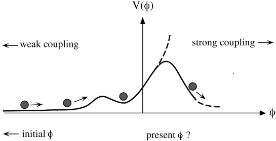
The basic idea of pre-big bang cosmology [600, 320, 321, 322] can then be illustrated as in Fig. 2.1, where the dilaton starts at very large negative values, rolling up a potential which, at the beginning, is practically zero (at weak coupling, the potential is known to be instantonically suppressed [90], ). The dilaton grows and inflates the Universe, until the potential develops some non-perturbative structure, which can eventually damp and trap the dilaton (possibly after some oscillations). The whole process may be seen as the slow, but eventually explosive, decay of the string perturbative vacuum (the flat and interaction-free asymptotic initial state of the pre-big bang scenario), into a final, radiation-dominated state typical of standard cosmology. Incidentally, as shown in Fig. 2.1, the dilaton of string theory can easily roll-up –rather than down– potential hills, as a consequence of its non-standard coupling to gravity.
A phase of accelerated evolution, sustained by the kinetic energy of a growing dilaton [600] (and possibly by other antisymmetric tensor fields [309, 178], in more complicated backgrounds) is not just possible: it does necessarily occur in a class of (lowest-order) cosmological solutions based on a cosmological variant of the (previously mentioned) -duality symmetry [600, 581, 478, 479, 561, 368, 582, 583, 319]. In such a way duality provides a strong motivation for (and becomes a basic ingredient of) the pre-big bang scenario first introduced in [600] and whose developments are the subject of this report.
The importance of duality for a string-motivated cosmology was indeed pointed out already in some pioneer papers [19, 429, 21, 110] based on superstring thermodynamics; the fact that our standard Universe could emerge after a phase of inflation with “dual” cosmological properties was also independently suggested by the study of string motion in curved backgrounds [316]. For future applications (see Section 8) we wish to recall here, in particular, the -duality approach to a superstring Universe discussed in [110] (see also [379]), in which all nine spatial dimensions are compact (with similar radius), and the presence of winding strings wrapped around the tori prevents the expansion of the primordial Universe, unless such winding modes disappear by mutual annihilation.
The probability of annihilation, however, depends on the number of dimensions. In it is so small that strings prevent the nine dimensions from expanding. If dimensions contract to the string size, string annihilation in the other is still so small that even they cannot expand. Only for is the annihilation probability in the remaining dimensions large enough, and the expansion becomes possible: this would give as the maximal number of large space dimensions (such a mechanism has recently been extended also to a more general brane–gas context, see Subsection 8.5).
This as well as the other, early attempts were based on Einstein’s cosmological equations, i.e. on gravitational equations at fixed dilaton. Taking into account the large-distance modifications of general relativity required by string theory, and including a dynamical dilaton, the target-space duality typical of closed strings moving in compact spaces can be extended (in a somewhat modified version) even to non-compact cosmological backgrounds [600, 479, 581, 582, 583]. Consider in fact a generic solution of the field equations of string theory (hence a point in our moduli space), which possesses a certain number of Abelian isometries (the generalization to non-Abelian isometries is subtle, see [207]). Working in an adapted coordinate system, in which the fields appearing in the solution are independent of -coordinates, it can then be argued [478] that there is an group that, acting on the solution, generates new ones (in other words, this group has a representation in that part of moduli space that possesses the said isometries).
Note that, unlike strict -duality, this continuous extension is not a true symmetry of the theory, but only a symmetry of the classical field equations. The corresponding transformations can be used to generate, from a given solution, other, generally inequivalent ones, and this is possible even in the absence of compactification. In the next subsections we will show in detail that such transformations, applied to a decelerated cosmological solution (and combined with a time-reversal transformation) lead in general to inflation, and we shall present various (low-energy) exact inflationary solutions, with and without sources, which may represent possible models of pre-big bang evolution. We shall consider, in particular, both scale-factor [600, 581, 583] and [478, 479, 561, 368, 319] duality tranformations, and we will discuss some peculiar kinematic aspects of such pre-big bang solutions.
2.2 Scale-factor duality without and with sources
We start by recalling that, in general relativity, the Einstein action is invariant under time reflections. It follows that, if we consider an isotropic, spatially flat metric parametrized by the scale factor ,
| (2.3) |
and if is a solution of the Einstein equations, then is also a solution. On the other hand, when the Hubble parameter flips sign;
| (2.4) |
Thus, to any standard cosmological solution , describing decelerated expansion and decreasing curvature (, ), time reversal associates a “reflected” solution, , describing a contracting Universe.
In string theory, the reparametrization and gauge invariance of conventional field theories are expected to be only a tiny subset of a much larger symmetry group, which should characterize the effective action even at lowest order. The string effective action that we shall use in this section, in particular, is determined by the usual requirement that the string motion is conformally invariant at the quantum level [347]. The starting point is the (non-linear) sigma model describing the coupling of a closed string to external metric (), scalar (), and antisymmetric tensor () fields. In the bosonic sector the action reads:
| (2.5) |
Here , , and are the coordinates spanning the two-dimensional string world-sheet (), whose induced metric is . The coordinates are the fields determining the embedding of the string world-sheet in the external (also called “target”) space, is the two-dimensional Levi-Civita tensor density, and is the scalar curvature for the world-sheet metric . We have included the interaction of the string with all three massless states (the graviton, the dilaton and the antisymmetric tensor) appearing in the lowest energy level of the spectrum of quantum string excitations (the unphysical tachyon is removed by supersymmetry [347]). We note, for further use, that the antisymmetric field is often called the Neveu–Schwarz/Neveu–Schwarz (NS-NS) two-form.
If we quantize the above action for the self-coupled fields , we can expand the loop corrections of the corresponding non-linear quantum field theory in powers of the curvature (i.e. in higher derivatives of the metric and of the other background fields) [347]. Such a higher derivative expansion is typical of an extended object like a string, and is indeed controlled by the powers of , i.e. of the string length parameter . At each order in , however, there is an additional higher genus expansion in the topology of the world-sheet metric, which corresponds, in the quantum field theory limit, to the usual loop expansion, controlled by the effective coupling parameter .
The conformal invariance of the classical string motion in an external background can then be imposed, at the quantum level, at any loop order: we obtain, in this way, a set of differential conditions to be satisfied by the background fields for the absence of conformal anomalies, order by order. At tree level in , and to lowest order in , such differential equations (in a critical number of dimensions) are [347]:
| (2.6) | |||
| (2.7) |
where cyclic permutations. By introducing the Einstein tensor, , the first equation can be rewritten in a more “Einsteinian form” as
| (2.8) |
and it can be easily checked that Eqs. (2.7), (2.8) can be derived by the -dimensional effective action
| (2.9) |
This action (possibly supplemented by a non-perturbative dilaton potential, and/or by a cosmological term in non-critical dimensions [347]) is the starting point for the formulation of a string-theory-compatible cosmology in the small-curvature and weak-coupling regime, , (see Section 8 for higher-order corrections).
For an illustration of scale factor duality it will now be sufficient to restrict our attention to the gravidilaton sector of the action (2.9) (setting e.g. ). We will consider an anisotropic Bianchi-I-type metric background, with homogeneous dilaton , and we will parametrize the action in terms of the “shifted” scalar field (see Section 1.4 for the notation). The field equations (2.7), (2.8) then provide a system of equations for the variables :
| (2.10) | |||
| (2.11) | |||
| (2.12) |
In the absence of sources only equations are independent (see for instance [308]; Eq. (2.10), in particular, represents a constraint on the set of initial data, which is preserved by the evolution).
The above string cosmology equations are invariant not only under a time-reversal transformation,
| (2.13) |
but also under a transformation that inverts any one of the scale factors, preserving the shifted dilaton,
| (2.14) |
and which represents a so-called scale-factor duality transformation [600, 581]. Note that the dilaton is not invariant under this transformation: if we invert, for instance, the first scale factors, the transformed dilaton is determined by the condition
| (2.15) |
Thanks to scale-factor duality, given any exact solution of Eqs. (2.10)–(2.12), represented by the set of variables
| (2.16) |
the inversion of scale factors then defines a new exact solution, represented by the set of variables
| (2.17) |
Consider in particular the isotropic case , where all the scale factors get inverted, and the duality transformation takes the form:
| (2.18) |
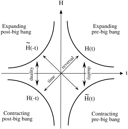
When the Hubble parameter goes into so that, to each of the two solutions related by time reversal, and , is also associated a dual solution, and , respectively (see Fig. 2.2). The space of solutions, in a string cosmology context, is thus richer than in the standard Einstein cosmology, because of the combined invariance under duality and time-reversal transformations. In string cosmology, a solution has in general four branches: . Two branches describe expansion (), the other two branches describe contraction (). Also, as illustrated in Fig. 2.2, for two branches the curvature scale () grows in time, so that they describe a Universe that evolves towards a singularity, with a typical “pre-big bang” behaviour; for the other two branches the curvature scale decreases, so that the corresponding Universe emerges from a singularity, with a typical “post-big bang” behaviour.
What is important, in our context, is that to any given decelerated, expanding solution, , with decreasing curvature, (typical of the standard cosmological scenario), is always associated an inflationary “dual partner” describing accelerated expansion, , and growing curvature, . This pairing of solutions (which has no analogue in the context of the Einstein cosmology, where there is no dilaton, and the duality symmetry cannot be implemented) naturally suggests a “self-dual” completion of standard cosmology, in which the Universe smoothly evolves from the inflationary pre-big bang branch to the post-big bang branch (after an appropriate regularization of the curvature singularity appearing in the lowest-order solutions).
As a simple example of the four cosmological branches, we may consider here the particular isotropic solution defined in the positive range of the time coordinate,
| (2.19) |
which is singular at and satisfies identically the set of equations (2.10) – (2.12). By applying a duality and a time-reversal transformation we obtain the four inequivalent solutions
| (2.20) |
corresponding to the four branches illustrated in Fig. 2.2. These solutions are separated by a curvature singularity at ; they describe decelerated expansion , decelerated contraction , accelerated contraction , accelerated expansion (the solution is accelerated or decelerated according to whether and have the same or opposite signs, respectively). The curvature is growing for , decreasing for . Note that the transformation connecting two different branches represents in this case not really a symmetry, but rather a group acting on the space of solutions, transforming non-equivalent conformal backgrounds into each other, like in the case of the Narain transformations [499, 500].
For further applications, it is also important to consider the dilaton evolution in the various branches of Eq. (2.20). Using the definition (1.23),
| (2.21) |
It follows that, in a phase of growing curvature (), the dilaton is growing only for an expanding metric, . This means that, in the isotropic case, the expanding inflationary solutions describe a cosmological evolution away from the string perturbative vacuum (), i.e. are solutions characterized by a growing string coupling, . The string perturbative vacuum thus naturally emerges as the initial state for a state of pre-big bang inflationary evolution. This is to be contrasted with the recently proposed “ekpyrotic” scenario [413], where the “pre-big bang” configuration (i.e. the phase of growing curvature preceding the brane collision that simulates the big bang explosion) is contracting even in the S-frame [414] and indeed corresponds to a phase of decreasing dilaton.
Note that in a more general, anisotropic case, and in the presence of contracting dimensions, a growing-curvature solution is associated to a growing dilaton only for a large enough number of expanding dimensions. To make this point more precise, consider the particular, exact solution of Eqs. (2.10)–(2.12), with expanding and contracting dimensions, and scale factors and , respectively:
| (2.22) |
This gives
| (2.23) |
so that the dilaton is growing if
| (2.24) |
We note, incidentally, that this result may have interesting implications for a possible “hierarchy” of the present size of extra dimensions, if we assume that our Universe starts evolving from the string perturbative vacuum (i.e. with initial ). Indeed, in a superstring theory context (), it follows that the initial number of expanding dimensions is , while only may be contracting. A subsequent freezing, or late-time contraction (possibly induced by quantum effects [131]), of dimensions will eventually leave only three expanding dimensions, but with a possible huge asymmetry in the spatial sections of our Universe, even in the sector of the “internal” dimensions (see Refs. [110, 11], and the discussion of Section 8.5, for a possible mechanism selecting as the maximal, final number of expanding dimensions in a string- or brane-dominated Universe).
The invariance of the gravidilaton equations (2.10)–(2.12) is in general broken by a dilaton potential , unless is just a function of . The invariance, however, is still valid in the presence of matter sources, provided they transform in a way that is compatible with the string equations of motion in the given background [319] (see the next subsection). In the perfect-fluid approximation, in particular, a scale-factor duality transformation is associated to a “reflection” of the equation of state [600].
Consider in fact the addition to the action (2.9) of a matter action , minimally coupled to the S-frame metric (but uncoupled to the dilaton), and describing an anisotropic fluid with diagonal stress tensor,
| (2.25) |
The field equations (2.8) are now completed by a source term
| (2.26) |
(in units in which ), and the cosmological equations (2.10)–(2.12) become
| (2.27) | |||
| (2.28) | |||
| (2.29) |
where we have introduced the “shifted” density and pressure
| (2.30) |
They are a system of independent equations for the variables . Their combination gives
| (2.31) |
which represents the usual covariant conservation of the source energy density. The above equations with sources are invariant under time reflection and under the duality transformation [600]
| (2.32) |
which preserves but changes in a non-trivial way, and“reflects” the barotropic equation of state, . Thus, a cosmological solution is still characterized by four distinct branches.
We will present here a simple isotropic example, corresponding to the power-law evolution
| (2.33) |
(see the next subsection for more general solutions). We use (2.27), (2.29), (2.31) as independent equations. The integration of Eq. (2.31) immediately gives
| (2.34) |
Eq. (2.27) is then satisfied, provided
| (2.35) |
Finally, Eq. (2.29) leads to the constraint
| (2.36) |
We then have a (quadratic) system of two equations for the two parameters (note that, if is a solution for a given , then also is a solution, associated to ). We have in general two solutions. The flat-space solution, , corresponds to a non-trivial dilaton evolving in a frozen pseudo-Euclidean background, sustained by the energy density of dust matter (), according to Eq. (2.28). For we obtain instead
| (2.37) |
which fixes the time evolution of and :
| (2.38) |
and also of the more conventional variables :
| (2.39) |
This particular solution reproduces the small-curvature limit of the general solution with perfect fluid sources sufficiently far from the singularity, as we shall see in the next subsection. As in the vacuum solution (2.19), there are four branches, related by time-reversal and by the duality transformation (2.32), and characterized by the scale factors
| (2.40) |
For , and we recover in particular the standard, radiation-dominated solution with constant dilaton:
| (2.41) |
describing decelerated expansion and decreasing curvature:
| (2.42) |
typical of the post-big bang radiation era. Through a duality and time-reversal transformation we obtain the “dual” complement:
| (2.43) |
which is still an exact solution of the string cosmology equations, and describes accelerated (i.e. inflationary) expansion, with growing dilaton and growing curvature:
| (2.44) |
(the unconventional equation of state, , is typical of a gas of stretched strings, see [315, 316] and the next subsection).
This confirms that, if we start with our present cosmological phase in which the dilaton is constant (in order to guarantee a constant strength of gravitational and gauge interactions), and we postulate for the early Universe a dual complement preceding the big bang explosion, then string theory requires for the pre-big bang phase not only growing curvature, but also growing dilaton.
In other words, string theory naturally suggests to identify the initial configuration of our Universe with a state asymptotically approaching the flat, cold and empty string perturbative vacuum, , . As a consequence, the initial cosmological evolution occurs in the small curvature () and weak coupling () regime, and can be appropriately described by the lowest order effective action (2.9) (see Fig. 2.3). The solutions (2.41) and (2.43) provide a particular, explicit representation of the scenario represented in Fig. 2.3, for the two asymptotic regimes of large and positive, Eq. (2.41), and large and negative, Eq. (2.43).

It should be mentioned, to conclude this subsection, that the invariance under the discrete symmetry group , generated by the inversion of scale factors, can be generalized so as to be extended to spatially flat solutions of more general scalar–tensor theories [143, 435], with the generic Brans–Dicke parameter , described by the action
| (2.45) |
The case corresponds to the string effective action. For , the equations of an isotropic and spatially flat background (with scale factor ) are invariant under the transformation , , where , and [435]
| (2.46) |
(when one recovers the transformation (2.18)). Similar symmetries are also present in a restricted class of homogeneous, Bianchi-type models [170] (but the presence of spatial curvature tends to break the scale-factor duality symmetry); for the Bianchi-I-type metrics, in addition, the discrete transformation (2.46) can be embedded in a continuous symmetry group.
It should be stressed, however, that when such generalized transformations do not necessarily associate, to any decelerated solution of the standard scenario, an inflationary solution with growing dilaton. In this sense, a self-dual cosmological scenario in which inflation emerges naturally from the perturbative vacuum seems just to be a peculiar prediction of string theory, in its low energy limit.
In the next subsection we will extend the discussion of this section to more general models of background and sources.
2.3 -covariance of the cosmological equations
The target-space duality introduced in the previous subsection is not restricted to the gravidilaton sector and to cosmological backgrounds, but is expected to be a general property of the solutions of the string effective action (possibly valid at all orders [561, 368], with the appropriate generalizations [477, 398]).
Already at the lowest order, in fact, the inversion of the scale factor is only a special case of a more general transformation of the global group which leaves invariant the action (2.9) for all background characterized by Abelian isometries, and which mixes in a non-trivial way the components of the metric and of the antisymmetric tensor (see [341] for a general review).
Such an invariance property of the action can also be extended to non-Abelian isometries [207], but then there are problems for “non-semisimple” isometry groups [314]. Here we shall restrict ourselves to the Abelian case, and we shall consider (for cosmological applications) a set of background fields which is isometric with respect to spatial translations and for which there exists a synchronous frame where , and all the non-zero components of (as well as the dilaton itself) are only dependent on time.
In order to illustrate the invariance properties of such a class of backgrounds under global transformations, we shall first rewrite the action (2.9) directly in the synchronous gauge (since, for the moment, we are not interested in the field equations, but only in the symmetries of the action). We set and find, in this gauge,
| (2.47) |
where
| (2.48) |
and so on [note also that means ]. Similarly we find, for the antisymmetric tensor,
| (2.49) |
Let us introduce the shifted dilaton, by absorbing the spatial volume into , as in Section 1.4:
| (2.50) |
from which
| (2.51) |
By collecting the various contributions from and , the action (2.9) can be rewritten as:
| (2.52) |
We can now eliminate the second derivatives, and the mixed terms containing , by noting that
| (2.53) |
Finally, by using the identity , we can rewrite the action in quadratic form, modulo a total derivative, as
| (2.54) |
This action can be set into a more compact form by using the matrix , defined in terms of the spatial components of the metric and of the antisymmetric tensor,
| (2.55) |
and using also the matrix , representing the invariant metric of the group in the off-diagonal representation:
| (2.56) |
( is the unit -dimensional matrix). By computing and we find, in fact,
| (2.57) |
so that the action can be rewritten as [478, 479]
| (2.58) |
We may note, at this point, that itself is a (symmetric) matrix element of the pseudo-orthogonal group, since
| (2.59) |
for any and . Therefore:
| (2.60) |
and the action can be finally rewritten in the form
| (2.61) |
which is explicitly invariant under global transformations preserving the shifted dilaton :
| (2.62) |
When , the matrix is block-diagonal, and the special transformation represented by corresponds to an inversion of the metric tensor:
| (2.63) |
so that . For a diagonal metric, in particular, , and the invariance under the scale factor duality transformation (2.18) is recovered as a particular case of the global symmetry (as already anticipated).
This invariance holds even in the presence of sources representing bulk string matter [319], namely sources evolving consistently with the solutions of the string equations of motion in the background we are considering. A distribution of non-interacting strings, minimally coupled to the metric and the antisymmetric tensor of an -covariant background, is in fact characterized by a stress tensor (source of ) and by an antisymmetric current (source of ), which are automatically -covariant).
In order to illustrate this important point we add to Eq. (2.9) an action describing matter sources coupled to and to , and we define
| (2.64) |
The variation with respect to the dilaton, to and gives then, respectively, Eqs. (2.7), Eq. (2.26) and the additional equation
| (2.65) |
For a background with spatial isometries, and in the synchronous gauge, such field equations can be written in matrix form using , and a new set of “shifted” variables defined as follows:
| (2.66) |
where and are matrices. In particular, the dilaton equation (2.7) takes the form
| (2.67) |
the component of Eq. (2.26) gives
| (2.68) |
while the spatial part of Eq. (2.26), combined with Eq. (2.65), can be written in the form
| (2.69) |
where is a matrix composed with and :
| (2.70) |
(see [319] for an explicit computation). By differentiating Eq. (2.68), using Eqs. (2.67), (2.69), and the identity
| (2.71) |
we obtain the generalized energy conservation equation, written in matrix form as
| (2.72) |
The covariance of the string cosmology equations is thus preserved even in the presence of matter sources, provided transforms in the same way as . In that case, the whole set of equations (2.67)–(2.69) is left invariant by the generalized transformation
| (2.73) |
where . This is indeed what happens if the sources are represented by a gas of non-self-interacting strings.
Suppose in fact that the matter action is given by the sum over all components of the string distribution, , where we use the action (2.5), and we choose the conformally flat gauge for the world-sheet metric (i.e. , ):
| (2.74) | |||||
Here and are the world-sheet coordinates, and . The variation with respect to and gives the tensors (2.66), which depend on the world-sheet integral of a form bilinear in . The variation with respect to gives the string equations of motion, the variation with respect to (before imposing the gauge) gives the constraints. If we have a solution of the equations of motion, in a given background , and we perform an transormation , the new solution is found to correspond to transformed matrices and , which combine to give [319]. The covariance is thus preserved, provided the matter sources transform according to the string equations of motion, which can themselves be written in a fully covariant form.
Let us now exploit this covariance to find more general solutions of the string cosmology equations, and more general examples of duality-related backgrounds corresponding to possible models for the pre-big bang scenario. Let us introduce a convenient (dimensionless) time-coordinate , such that
| (2.75) |
( is a constant length). Assuming that the equation of state can be written in terms of a given matrix , such that
| (2.76) |
we can integrate a first time Eqs. (2.67)–(2.69), also with the help of the identity (2.71). The result is [322]
| (2.77) | |||
| (2.78) |
where
| (2.79) |
(a prime denotes differentiation with respect to , and is an integration constant).
By exploiting the fact that is a symmetric matrix, , and that , because of the definition of (see [319]), the above equations can be formally integrated to give
| (2.80) | |||
| (2.81) |
where is a constant, a constant symmetric matrix, and denotes the “-ordering” of the exponential. For any given “equation of state” , providing an integrable relation for , according to Eq. (2.76), the general exact solution of the low-energy string cosmology equations (for space-independent fields and vanishing dilaton potential) is then represented by Eqs. (2.79)–(2.81).
Such solutions contain in general singularities for the curvature and the string coupling, in correspondence with the zero of . Near the singularity (i.e., for ) the contribution of the matter sources becomes negligible with respect to the curvature terms in the field equations (as,in general relativity, for the Kasner anisotropic solutions [439]), and one recovers the general vacuum solutions presented in [478]. This can be shown in general for any background , and any kind of matter distribution [322]; for further applications, however, it will be sufficient to report here the case of anisotropic but torsionless () backgrounds, with diagonal metric , and fluid sources with a barotropic equation of state, as in Eq. (2.25).
In this case we obtain, from the previous definitions,
| (2.82) |
where
| (2.83) |
are the zeros of , and , are integration constants. The general solution (2.79)–(2.81) reduces to [321]
| (2.84) | |||
| (2.85) | |||
| (2.86) |
where
| (2.87) |
and , are additional integration constants.
This solution has two curvature singularities at . Near the singularity the sources are negligible, and one recovers the anisotropic vacuum solution of string cosmology in critical dimensions [600, 490]. Indeed, for , one finds from Eqs. (2.75) and (2.86) that , and the solution reduces to
| (2.88) |
where
| (2.89) |
In the large- (small-curvature) limit, on the contrary, the relation between and cosmic time is , and the solution (2.84)–(2.86) behaves like (for )
| (2.90) |
We may note, in general, that the relative importance of the matter sources with respect to the curvature is measured by the ratio (see Eq. (2.68),
| (2.91) |
(normalized in such a way that one recovers the usual critical energy–density ratio, , when is constant and the metric is isotropic). It follows that when , while in the opposite limit , dominated by the matter sources, goes to a constant,
| (2.92) |
which is obviously for the isotropic, radiation-dominated background with and constant dilaton.
Now it can easily be checked that, in the isotropic case , , the vacuum solution (2.20) and the matter-dominated solutions (2.38), (2.39) presented in the previous subsection can be directly recovered from Eqs. (2.88) and (2.90), respectively. As before, we have invariance under time reflections and under the duality transformation , . In addition, we can now perform more complicated transformations to find anisotropic and non-diagonal pre-big bang backgrounds [309] (the possibility of singularity-free solutions, in this context, will be discussed in Section 8). It should be stressed, however, that the “ complement” of a standard cosmological solution is in general associated to the introduction of an effective viscosity in the matter stress tensor, as pointed out in [319].
To conclude this subsection let us finally report the cosmic-time and conformal-time parametrization of the isotropic solutions, in the asymptotic limit of large and small curvature, both in the S-frame and in the E-frame.
The small-curvature limit, dominated by a perfect fluid with , has been given in cosmic time in Eqs. (2.38), (2.39). In the conformal time gauge, defined by , we obtain
| (2.93) |
Instead, the vacuum, dilaton-dominated limit (2.20) becomes, in conformal time,
| (2.94) |
In the E-frame, the scale-factor and the curvature parameters are obtained through the transformation (1.8), (1.11) (the conformal time is obviously the same in both frames). The small-curvature limit (2.38), (2.39) becomes, in cosmic time,
| (2.95) |
where
| (2.96) |
In conformal time,
| (2.97) |
The vacuum, dilaton-dominated limit (2.20) becomes, in cosmic time,
| (2.98) |
and
| (2.99) |
in conformal time.
The above solutions will be used to discuss the kinematics of the phase of pre-big bang inflation (in the next subsection), and to compute the corresponding amplification of the quantum fluctuations (see Section 4). For the discussion of more general homogeneous solutions (see for instance [61, 58, 60]), we refer the reader to the existing literature, and in particular to the detailed phase-space analysis of the string cosmology equations performed including non-trivial two-form potentials (), moduli fields, spatial curvature, anisotropy, and a cosmological constant in both the matter and the gravidilaton parts of the action [85, 86, 87].
2.4 Kinematics of pre-big bang inflation
The symmetry properties of the string effective action suggest a “self-dual” cosmological scenario, in which the Universe evolves from an initial configuration approaching (asymptotically) the string perturbative vacuum (, ). Such a state, on the other hand, is particularly appropriate to provide the initial conditions, because it is unstable with respect to the decay into an inflationary phase eventually driven by the dilaton kinetic energy. A small inhomogeneity of the perturbative vacuum is indeed sufficient to trigger inflation, as we shall discuss in Section 3. Or, keeping homogeneity, a small perturbation represented by a constant non-zero energy density is also sufficient.
In the first models of pre-big bang evolution [320, 322], such a perturbation was generated by a (sufficiently diluted) gas of fundamental strings, as its presence tends to enhance the instability of the full system (background fields plus mattere sources). Suppose in fact that we look for self-consistent, simultaneous solutions of the gravidilaton background equations (2.27)–(2.29) and of the string equations of motion (in the same background), obtained from Eq. (2.74) with :
| (2.100) |
Given a consistent embedding , the sum over all the stress tensors of each individual string,
| (2.101) |
(after an appropriate averaging procedure) provides the effective sources to be inserted into the background equations.
The above system of string and background equations can be solved in a perturbative way [303, 304], by imposing the string perturbative vacuum as asymptotic initial conditions at . To zeroth order, the background manifold is flat, and the string solutions are characterized by , , corresponding to a pressureless effective stress tensor, const, (dust matter, in the perfect-fluid approximation).
To first order, the background solution thus corresponds to the case and to the negative branch () of Eqs. (2.84)–(2.86), namely
| (2.102) |
( are integration constants). Note that since const, and that we have performed a time translation to shift the singularity from to the origin. Note also that, at , the metric is flat and only the dilaton is rolling, , sustained by a constant (pressureless) string energy density const, (consistently with the chosen initial conditions).
The string equation of state keeps unchanged until const, namely for . When approaches the critical scale , however, the scale factors start rolling and evolve towards a final (expanding or contracting) accelerated configuration
| (2.103) |
reached asymptotically for . When , therefore, the horizon starts shrinking (see Section 1.3) and we know, in that regime, that extended objects become “unstable” [552, 269, 271]. In the case of string matter, in particular, we know that the asymptotic solutions of the string equations of motion, outside the horizon [315, 316], are characterized by , for accelerated expansion (), and by , for accelerated contraction (). As a consequence, the string stress tensor (2.101) satisfies, respectively, the conditions
| (2.104) |
corresponding to the radiation equation of state () for accelerated contraction, and to its dual () for accelerated expansion. In both cases, the string pressure triggers a regime of positive feedback, which enhances the instabilitys and pushes the system (background fields plus sources) even further away from the string perturbative vacuum [316, 320, 303, 304].
When , however, the contribution of the matter sources becomes negligible in the field equations: a first differentiation of Eq. (2.102) gives in fact
| (2.105) |
and then for . So, even if the string pressure tends to deviate from its initial vanishing value, its dynamical effects eventually become negligible when the background enters the dilaton-dominated regime. The solution (2.102) thus represents a reliable description of the coupled system background plus string sources, both in the and limits, namely in the initial and final regimes, sufficiently far from the critical time scale [304].
What is important, for the purpose of this section, is that the phase of pre-big bang inflation, at low energy, is in general characterized by two possible (connected) branches: an initial (model-dependent) phase in which matter (like string, or other sources) are possibly important, and a second “vacuum” phase dominated by the dilaton kinetic energy. The validity of the low energy solutions stops of course at the string scale, . At that point the higher order (loop and ) quantum corrections come into play, but inflation can nonetheless continue during a phase of constant curvature and linearly growing dilaton [308], appearing as late-time attractor in the high-curvature regime (see Section 8).
So, in spite of the fact that the inflationary epoch of the pre-big bang scenario is often referred to as the vacuum, dilaton-driven phase appearing in the low energy solutions, it is important to stress that the total pre-big bang inflationary period possibly contains also a phase of “late inflation” at high curvature (as also stressed in [467]), and a phase of “early inflation” driven by matter sources (as also stressed in [325]). To discuss the main kinematic aspects of pre-big bang inflation, however, it will be sufficient to concentrate our attention on the dilaton-driven, isotropic vacuum solutions given by Eq. (2.20) (or by Eq. (2.94), in the conformal-time parametrization).
For a quantitative estimate of the duration of the inflationary period we observe that the ratio , determined by the flatness problem as in Eq. (1.2), also controls the solution of the horizon problem through the ratio
| (2.106) |
and that, for a power-law metric , such a ratio scales linearly with respect to the conformal time coordinate,
| (2.107) |
Also, we shall assume that the standard radiation era can be extended back in time down to the Planck scale, and that it is immediately preceded by a phase of accelerated expansion. At the beginning of the radiation era the horizon size is then controlled by the Planck length , while the proper size of the homogeneous and causally connected region inside our present Hubble radius, rescaled down according to the decelerated evolution of the standard scenario, is unnaturally larger than the horizon by the factor (as already remarked in Subsection 1.1). During the inflationary epoch the ratio must thus increase by at least a factor , so as to push the homogeneous region outside the horizon, by he amount required by the subsequent decelerated evolution. This determines the condition
| (2.108) |
where and mark, respectively, the beginning and the end of the inflationary period.
Let us now suppose, for simplicity (and for a more direct comparison between the pre-big bang and the standard inflationary scenarios), that at the end of inflation the dilaton immediately freezes out, and that the string and Planck lengths have already comparable sizes at (which means , according to Eq. (2.2)).
If we go back in time during a dilaton-dominated phase of isotropic superinflation,
| (2.109) |
starting from the string/Planck scale (), it follows from (2.108) that the scale factor is at most reduced by the factor , corresponding to a homogeneous region, which, at the beginning of inflation, is still very large in string units, i.e. at least
| (2.110) |
(i.e. for ). This is to be contrasted with the case of standard (although not fully realistic) de Sitter inflation, , where, going back in time, the scale factor during inflation is reduced by the factor , so that the size of the initial homogeneous region is just , like the horizon, which stays frozen during inflation.
The contrast is even more striking if the initial size (2.110) is expressed in Planck units, since, at the beginning of inflation, the string coupling –and thus the Planck length – is reduced with respect to its final value () by the factor
| (2.111) |
so that the lower bound (2.110) for the size of the initial region can be written as
| (2.112) |
(i.e. for ). This, by the way, is exactly the initial size evalued in the E-frame where is a constant, and the pre-big bang phase is represented as a contraction, according to Eq. (2.99).
One might think that, in such a case, the situation is not much better than in the case of non-inflationary cosmology, where one finds that the initial size of the homogeneous part of our Universe is greater than [395]. It should be noted, however, that without inflation the initial homogeneous region has to be much bigger than the horizon. In the pre-big bang scenario, on the contrary, the initial homogeneous region is large in Planck or string units, but not larger than the horizon itself [287]. Indeed, during superinflation, the horizon scale shrinks linearly in cosmic time. As we go backwards in time, in the particular example that we are considering, the horizon increases by the factor , so that, at the beginning of inflation, , i.e. the initial horizon size is just the same as that of the homogeneous region (2.110) (as also illustrated in Fig. 1.3).
In this sense, the initial state of pre-big bang inflation is similar to the one of the standard inflationary scenario. In one case, however, the initial horizon is large in Planck units; in the other case it is of order , as an obvious consequence of the different curvature scales at the beginning of inflation. The question about the naturalness of the initial conditions (see the next section) thus seems to concern the initial unit of length used to measure the size of the initial homogeneous domain: Should we use the Planck (or string) length, or the classical radius of the causal horizon?
The Planck length certainly provides natural units for the size of the initial homogeneous patches when initial conditions are imposed on a cosmological state approaching the high-curvature, quantum-gravity regime. In the pre-big bang scenario, however, initial conditions are to be imposed when the Universe is deeply inside the low-curvature, weak-coupling, classical regime. In that regime, the Universe does not know about the Planck length, and the causal horizon seems to provide a natural candidate for the initial homogeneity scale. It should be noted, to this purpose, that the formation of a large homogeneous domain is not prevented by the amplification of quantum fluctuations [344]. However, classical inhomogeneities, not normalized to a vacuum fluctuation spectrum, may require a constraint on the duration of inflation stronger than Eq. (2.108), as recently pointed out in [129].
Note also that a large (homogeneous) Hubble horizon, if we assume the saturation of the holographic bound [376] applied in a cosmological context [605], implies a large initial entropy (horizon area in Planck units) and corresponds, in a quantum context, to a small probability that such configuration be obtained through a process of quantum tunnelling (proportional to ). In the context of the pre-big bang scenario, however, quantum cosmology effects, such as tunnelling or reflection of the Wheeler–De Witt wave function, are expected to be important towards the end of inflation, and not the beginning, as they may be effective to exit, eventually, from the inflationary regime (see Section 9), not to enter it, and to explain the origin of the initial state. A large entropy of the initial state, in the weakly coupled, highly classical regime, can only correspond to a large probability of such a configuration (proportional to ), as expected for classical and macroscopic configurations.
The naturalness of the initial conditions will be discussed in Section 3. Here we note, to conclude this subsection, that an initial state characterized by a set of large (or small) dimensionless parameters, determined by a large initial horizon scale , is an unavoidable aspect of all models in which inflation starts at scales smaller than Planckian. In the standard scenario, where observational tracks of what happened before the Planck epoch are washed out, one may regard as unnatural [395] having an initial homogeneity scale of order whenever is very small in Planck or string units. In the context of the pre-big bang scenario, however, the phenomenological imprint of the Planck epoch is not necessarily washed out by a long and subsequent inflationary phase. The pre-Planckian history may become visible, and the sub-Planckian initial conditions are accessible, in principle, to observational tests, so that their naturalness can also be analysed with a Bayesan approach, in terms of “a posteriori” probabilities, as in [130] (see also [171, 172, 169] for a discussion of “generic” initial conditions in the pre-big bang scenario).
2.5 Frame-independence: Which is the “right” metric?
As already stressed in the previous discussion, and explicitly computed in Section 1.3, an S-frame inflationary solution of the string cosmology equations, when transformed to the E-frame, tends to describe a phase of accelerated contraction. This is strictly true only for isotropic backgrounds because, if the metric is anisotropic, and there is a large enough number of (S-frame) contracting dimensions, the other dimensions may keep expanding (and accelerated) in both frames.
Consider, for instance, the S-frame vacuum solutions (2.22), corresponding to expanding and contracting dimensions. When expressed in terms of the E-frame metric , and in the cosmic time gauge, through the transformation
| (2.113) |
(which generalizes to the anisotropic case the transformations of Eqs. (1.8), (1.11)), the solution becomes
| (2.114) |
The expanding part of the solution thus remains expanding (and inflationary ) even in the E-frame, provided . Note that, for , this condition is compatible with the condition of growing dilaton, , only for .
However, isotropic () metrics in the E-frame are contracting. This does not represent a difficulty for the pre-big bang scenario because the contraction is accelerated, , and thus corresponds to a phase in which the ratio decreases in time, as required for the solution of the horizon/flatness problems (see Sections 1.3 and 2.4). In particular, if the phase of accelerated expansion is long enough to solve the problems in the S-frame, according to Eq. (2.108), then the problems are also solved in the E-frame [321], since the conformal time is the same in both:
| (2.115) |
Furthermore, as we will see in Section 4.1, the spectral distribution of the metric fluctuations amplified by inflation is also the same in both frames [321, 322].
Such a frame independence of the inflationary aspects of the pre-big bang solutions also extends to the string-driven (and, more generally, matter-dominated) solutions presented in the previous subsection.
Suppose, in fact, that we start, at some initial time , with a distribution of strings characterized in the S-frame by a packing factor (average distance/average size) of the order of unity, and with sufficiently small interactions to represent a perfect fluid source for the superinflationary solution (2.38), (2.39), with . In the S-frame, where the metric is expanding, the perfect-fluid approximation is also valid at any subsequent time , as the number of strings per unit of string volume is diluted in time by the factor . In the E-frame the metric is contracting, but the string’s proper size shrinks with time as . As a consequence, the number of strings per unit of string volume scales as , and it is again diluted as time goes on, exactly by the same amount as in the S-frame [322].
With similar arguments it can be shown that the heating up of the string gas with respect to the radiation, which is easy to understand in the S-frame where the metric is expanding and the radiation is redshifted, also occurs in the E-frame, in spite of the fact that the radiation is blueshifted because of the contraction [321].
Using the standard thermodynamical arguments (see for instance [619]) we find indeed, for the perfect-fluid sources with , generating the solution (2.38), that their temperature satisfies . On the other hand, . In the S-frame the radiation () is thus supercooled and diluted with respect to the (string) sources that drive inflation (),
| (2.116) |
since the metric is expanding.
In the E-frame the fluid sources satisfy a modified conservation equation,
| (2.117) |
(the dots refer to the E-frame cosmic time ), obtained from Eq. (2.31), with defined in Eq. (2.96). The radiation, which has a traceless stress tensor, still evolves adiabatically, but now its temperature is blueshifted because of the contraction: . The effective temperature of the other matter sources is also blueshifted, however, and using thermodynamical arguments we obtain [321], from Eq. (2.117):
| (2.118) |
For the sources of the inflationary S-frame expansion we have , so that even in the E-frame the above ratio is growing, with a corresponding cooling down and dilution of the radiation density (with respect to the density of the inflationary sources).
There is thus a complete frame-independence for the physical effects of the inflationary solutions of the pre-big bang scenario. This can also be understood as an invariance of physics under a local field redefinition. Different frames are just related by a local (field-dependent) conformal transformation of the metric. No physical observables should depend on it, and this is what we shall find whenever we push a calculation to its very end (see also [20] for a recent discussion of this point). Further help is provided by the fact that, at late times, when the dilaton is frozen, all frames actually coincide.
Yet it is true that, in developing some physical intuition, there are important kinematical differences in different frames, as also stressed by the examples illustrated before. Inflation in the S-frame, for instance, can be represented as gravitational collapse in the E-frame (see the next section). We think that the S-frame (whose metric coincides with the sigma-model metric to which fundamental strings are directly coupled, see Section 2.2) is the one offering the simplest intuitive picture of how things evolve and work. The following three main points support this attitude.
The first point concerns the ultraviolet cut-off. The string metric is the one in which the ultraviolet cut-off of string theory is kept fixed, i.e. does not depend on the dilaton (at least in perturbation theory). This can be easily seen from the form of the tree-level action in the S-frame, in , in which we include a typical higher-derivative correction, :
| (2.119) |
Obviously, higher-derivative corrections become relevant, in this frame, as soon as and independently of . By contrast, the equivalent E-frame action would read:
| (2.120) |
indicating that higher-derivative corrections become relevant at , which is again the (dilaton-dependent) string scale expressed in Planck units.
The second point concerns masses. Tree-level string masses are dilaton-independent in the S-frame, but depend on in the E-frame since the S-frame relation becomes in the E-frame.
The third point concerns couplings. It is only an illusion that, by going to the E-frame, we make the Newton constant dilaton-independent. The physical quantity is not so much Newton’s constant but the gravitational force, say between two heavy strings. The force will be proportional to . In the S-frame, masses are dilaton-independent and , while, in the E-frame, is fixed but all masses scale like . The same physical result is obtained for the gravitational force but, clearly, it is much more economical to attribute the dilaton dependence of Newton’s force to Newton’s constant rather than to a universal dilaton dependence of all masses. We think that this is a good example of how physics is frame-independent, while our own physical intuition may prefer one frame to the other.
For all these reasons we shall interpret our results mainly in the string frame. Nonetheless, we shall often use other frames at intermediate stages of the calculation, to make it as simple as possible.
3 Initial conditions
We have already mentioned that, in standard non-inflationary cosmology, initial conditions have to be fine-tuned to an incredible accuracy in the far past (i.e. at s), or else it is impossible to explain some of the most striking properties of today’s Universe, such as its homogeneity and flatness.
In the pre-big bang scenario, having extended time to the past of the big bang event can certainly help solving the fine-tuning problems of standard cosmology: after all, most of these come from a “shortage of time” for things to happen early on after the big bang. Yet it is important to discuss the conditions under which a pre-big bang phase can naturally generate a patch that can evolve into the Universe we live in. In other words: What does the fine-tuning problem look like if, accepting hints from scale-factor duality, we assume perturbative, yet generic, initial conditions?
In this section we shall address this kind of questions by considering, for simplicity, a class of space-times endowed with a regular (time-like and null) asymptotic past, and by imposing on these geometries a condition of asymptotic-past-triviality (APT) (see Subsection 3.2). We are aware of the fact that this is already a schematization of a more general set-up where one would simply assume that the Universe, almost everywhere and almost all the time, is in a chaotic, highly entropic perturbative state in which the arrow of time itself is ill-defined. Within such a more general set-up a mechanism for generating a low-entropy subsystem has to be found, so that, within this subsystem, a time arrow (the direction of increasing entropy) can possibly be identified, and the organized Universe we happen to be living in can develop.
We shall argue in Subsection 3.3 that such a mechanism can be identified in the well-known phenomenon of gravitational collapse, and that the low-entropy region corresponding to our own Universe lies in the interior of the closed trapped surface that emerged from the collapse. We shall illustrate in Subsection 3.4 the particular cases of spherical and planar symmetry, comment on the problem of chaotic oscillations in Subsection 3.5, and finally present our conclusion on the fine-tuning problem in Subsection 3.6.
In our simplified approach we will treat one of these regions as representing, by itself, the full space-time manifold. Such a simplifying procedure is by no means new in general relativity: asymptotic flatness (asymptotic spatial triviality, in our terminology) is often assumed in order to prove rigorous theorems. Yet, causality guarantees that the collapse of a star within our galaxy can only depend on local conditions, and this allows for a simplified treatment of the problem.
In a similar spirit we shall assume that the dynamics that gave rise to our Universe can be approximately described by a space-time with an asymptotically trivial past. Thanks to gravitational instability, this evolved towards the formation of a closed trapped surface and of a space-like singularity of the big bang type. Assuming that the actual singularity is avoided, thanks to string corrections to general relativity, this process may give rise, eventually, to a (post-big bang) phase resembling the one of standard hot big bang cosmology.
In the next subsection, to approach the question of whether our present Universe may arise from generic initial conditions, we will relax the homogeneity assumption adopted in Section 2 and consider more general solutions of the string cosmology equations.
3.1 Quasi-homogeneous and inhomogeneous solutions
If we want to explain the large-scale homogeneity and isotropy of our Universe out of a cosmological phase preceding the big bang, we have to consider the case of non-homogeneous cosmologies with the hope to find homogeneity, isotropy, and flatness as asymptotic features of late-time attractors. The question, in particular, is how to obtain space-time manifolds where spatial gradients are subdominant with respect to time derivatives, starting from initial conditions in which they are of the same order. In a rather commonly used terminology, we would like to see “velocity-dominated” cosmologies emerge, at late times, from non-velocity-dominated initial conditions. This is what ordinary, slow-roll inflation supposedly does.
If we start from very generic inhomogeneous conditions, it is conceivable that, as in the case of chaotic inflation [440], only some spatial patches will end up exhibiting the required homogeneity and flatness to be consistent with our Universe, while inhomogeneity and anisotropy will prevail almost everywhere else. In the context of such a type of background evolution it is clear that, as a necessary preparatory exercise, we need to understand the nature of solutions that are not too inhomogeneous, leaving momentarily aside the problem of showing how patches of this kind may emerge at late times.
Such a program was started in [604] and further extended in [135]. The analysis performed in [604] was based on the general equations for the gravidilaton system in , together with the assumption of regularity at past infinity. It was shown that, on a constant-time hypersurface (defined in the synchronous gauge), sufficiently isotropic initial patches with and with a growing dilaton would inevitably expand, in the S-frame, and evolve towards homogeneity and strong coupling. Within those patches, a reliable expansion in spatial gradients [76] can be justified, the evolution quickly becomes velocity-dominated, and a Kasner-like singularity is approached according to the following generalization of the solution (2.88), (2.89):
| (3.1) |
If the above equations represented a general quasi-homogeneous solution, the generalization of scale-factor duality would be explicitly respected in the form (for any subset of indices ), while keeping all and fixed. However, the momentum constraints still have to be imposed on Eq. (3.1): they are trivial in the homogeneous case, but quite non-trivial in the presence of spatial gradients. These constraints preserve the simplest scale-factor duality [ for all ], but explicitly break its generalization [135]. The full symmetry is expected to be recovered as the solution approaches the singularity.
The (S-frame) local expansion rate, for the above metric, is given by the trace of the volume expansion tensor [616],
| (3.2) |
where is the unit time-like vector normal to the (space-like) homogeneity hypersurfaces. Under the Kasner constraint of Eq. (3.1), it is clear that the maximal rate of expansion is reached where all are equal and negative [604]. Hence the most isotropic patches are inflated most during this Kasner-like phase, suggesting that most of the space becomes fairly homogeneous and isotropic. This is true in spite of the fact that, unlike in ordinary inflation, the modulus of the shear tensor [616],
| (3.3) |
is not washed away as a Kasner-like singularity is approached [425] (unless higher-order corrections play an important role in this respect [334]).
In a subsequent work [135] these arguments were generalized in several directions. First, the equations were extended to an arbitrary number of dimensions, showing that in no qualitatively new results emerge: in particular there is no critical value of below which the phenomenon of BKL oscillations (to be described in Subsection 3.5) takes place. Secondly, quasi-homogeneous solutions were constructed with the inclusion of the NS-NS two-form : again, they look very similar to the known homogeneous solutions, provided the exponents are allowed to depend on space. The only non-trivial point consists, again, in imposing the momentum constraints that explicitly break symmetry.
The case of a quasi-homogeneous axion field in was also considered in [135]. Since the axion and are related by a (Poincaré) duality transformation that mixes space and time, this case is genuinely different from the one discussed above. Actually, the case of a homogeneous axion shows interesting new features, such as the blowing up of the dilaton both at very late and at very early times. These results, however, have to be taken with much precaution since some of the approximations may break down before such strong-coupling regimes are entered.
In [135] a conjecture was made that, as one approaches past infinity, there is a wide basin of attraction towards a trivial Milne geometry, which is nothing but a wedge of empty, flat Minkowski space in convenient coordinates. If this conjecture were true, we would conclude that the asymptotic past of pre-big bang cosmology is indeed trivial. However, the conjecture was proved not to be quite correct [168, 424], through the construction of exact inhomogeneous solutions of various kinds. Only some of them exhibit a Milne-like behaviour at very early times, while, more often than not, the asymptotic past consists of weakly interacting waves, endowed with the symmetries of the solutions, travelling on top of a trivial background [168, 424, 630]. Examples of this kind were constructed by various techniques.
In the case of cylindrical symmetry, exact, non-homogeneous and anisotropic solutions, containing both a dilaton and an axion fields, were already discussed in [62]. Up to a trivial time-reversal transformation, those solutions approach, near the late-time, a special case of the background (3.1), while, at very early times, an oscillatory behaviour prevails. The authors of [62] have also discussed symmetry properties of the solutions under duality transformations.
Inhomogeneous, cylindrical backgrounds for the bosonic massless modes of heterotic and type-IIB superstrings have also been obtained [248] by applying - and -duality transformations (as well as the usual Geroch transformations) to vacuum solutions of the Einstein equations exhibiting a two-dimensional group () of Abelian isometries. The inhomogeneous, string theory version of the Mixmaster (Bianchi-IX-type) cosmology, in particular, has been presented in [248]. Other inhomogeneous Einstein–Rosen string cosmologies were studied with a similar technique in [168], by applying the global duality symmetries of the superstring effective action to homogeneous models of Bianchi--type. Again, in these solutions, the conjecture of an asymptotic-past Milne metric is not usually satisfied. New inhomogeneous string cosmologies were also obtained in [437] by applying a discrete (mirror-like) symmetry of the string effective action to to vacuum solutions of general relativity.
On a more phenomenological ground, an interesting model containing a spherically symmetric inhomogeneity was studied at the non-perturbative level in [63]. Such a treatment allows the investigation of primordial black hole formation in string cosmology, an issue that we shall reconsider in the context of tensor perturbations in Section 5 (see also [438]). The question of how robust the existence of inflationary solutions is, in the presence of various axion-like backgrounds, was addressed in [249]; it was shown that in some cases the parameter space leading to inflation shrinks down to the empty set. Such a phenomenon may well be related to the generic existence of chaos and BKL oscillations, which will be discussed later, in Subsection 3.5.
The question of the asymptotic-past behaviour of inhomogeneous string cosmology was addressed in general in [424] within space-times, admitting two Abelian space-like Killing vectors. Once more, the asymptotic past, rather than empty and Milne-like, was found to contain weakly interacting waves. The inclusion of a Maxwell field was finally considered in [630]: even in this case, while the behaviour near the singularity is Kasner-like, the asymptotic past is filled with weakly interacting gravitational, dilatonic, and electromagnetic waves.
As a general remark all these special, exact, non-homogeneous solutions (and general, quasi-homogeneous solutions) can shed important light on the evolution of perturbations discussed in Sections 4–7, in particular when perturbation theory becomes inadequate. We shall occasionally make use of this connection later in this report. The conclusion that we wish to draw, for the time being, is that a simple structure in the asymptotic past (although not necessarily as trivial as Milne’s) can be consistently assumed for the generic solution. This suggests to replace the assumption of past regularity by a somewhat stronger postulate, that of asymptotic past triviality. Such a concept will be introduced and developed in the rest of this section.
3.2 Asymptotic past triviality and symmetries
We start from the general postulate that the pre-collapse, pre-big bang evolution of the Universe can be described in terms of the low-energy, tree-level action of string theory. Taking a generic closed superstring theory, this reads (see Section 2):
| (3.4) |
where is the (three-form) field strength associated with the antisymmetric tensor . A further simplification comes from assuming that we are dealing with so-called critical superstring theory, the case in which the tree-level (and actually the all-order-perturbative) cosmological constant vanishes. This requires a total of space-time dimensions [347]. If there will indeed be an effective cosmological constant preventing the existence of any low-curvature solution of the field equations.
Equation (3.4) receives corrections either when curvatures become , or when the coupling becomes . If such corrections are both negligible, it sometimes becomes useful to perform a change of variable by going to the E-frame, already introduced in the previous sections. In general, this is done by defining [576, 616]:
| (3.5) |
Using the Einstein metric (and dropping the tilde), the result for the action (3.4) is simply:
| (3.6) |
where is the present value of the Planck length, if we take to coincide with the present (constant) value of the dilaton.
Although the use of the E-frame could simplify some calculations, and we shall see examples of this below, it should be kept in mind that the form of the corrections is no longer so simple. For instance, as already stressed at the end of Section 2, higher-derivative corrections become important when the E-frame curvature is , i.e. when it reaches a dilaton-dependent critical value. Similarly, having a constant Newton “constant” in this frame is a mere illusion, because (even tree-level) string masses now depend upon (as already illustrated in Subsection 2.5). For these reasons, although physical results are frame-independent, we shall always describe them with reference to the original S-frame metric in which the string length is constant.
Let us finally remark that the two frames coincide today if the dilaton is eventually fixed at its present value . Similarly, as we shall see, the assumption of APT leads to a very large and negative value of the initial dilaton which, if finite, would also allow the identification of the two frames in the far past. However, the two E-frames that coincide with the S-frame at differ from each other by an enormous conformal factor, i.e. by a huge blowing-up of all physical scales.
The classical equations that follow from varying (3.4) or (3.6), besides being generally covariant, are also invariant under a two-parameter group of (global) transformations acting as follows:
| (3.7) |
where and are constant parameters (using general covariance, the latter symmetry is also equivalent to an overall rescaling of all the coordinates). Indeed, both actions are simply rescaled by a constant factor under this group. Note that these two symmetries depend crucially on the validity of the tree-level, low-energy approximation, and on the absence of a cosmological constant. Loop corrections clearly spoil invariance under dilaton shifts, while lower-derivatives (a cosmological constant) or higher-derivatives () corrections spoil invariance under a rescaling of the metric. The importance of dealing with critical superstring theory now becomes evident: if wewould consider non-supersymmetric string theories, a cosmological constant would almost certainly be generated at some finite order of the loop expansion, which would change completely the large-distance properties and would spoil the symmetries of the field equations.
The immediate consequence of the above two symmetries is that solutions of the field equations depend on two free parameters, a dimensionless one related to the overall value of , and a dimensionful one corresponding to an overall length scale. As a consequence, neither the value of the fundamental string length nor that of the Planck length are of relevance to the classical solutions. The importance of this point on the issue of fine-tuning will become clear later in this section.
Only if (and when) the solutions are driven into the high-curvature regime will higher-derivative corrections (involving the string length) will become relevant and break scale invariance. The analysis presented in this section can only be trusted up to this point, or until the strong coupling regime is reached. Which of the two limitations will be reached first depends, in turn, on the two above-mentioned classical moduli. For sufficiently small initial coupling the high-curvature regime is encountered first, while, for sufficiently small initial curvature, the opposite is true. Both possibilities will be discussed in the last part of this report (see Section 8).
As already mentioned, the way we now introduce (and exploit) the concept of APT in string cosmology parallels the familiar use of “asymptotic flatness” in general relativity [94, 546, 514]. In both cases some assumption of asymptotic simplicity is made, the asymptotic past in our case, spatial infinity in the more familiar case. It seems indeed physically (and philosophically) satisfactory to identify the beginning with simplicity. However, simplicity should not be confused with complete triviality: a rigorously empty and flat Universe, besides being uninteresting, is also very special, i.e. non-generic. By contrast, asymptotically trivial Universes, though initially simple, are also generic in a precise mathematical sense that we shall now discuss.
In the weak-coupling, small-curvature, low-energy regime under consideration, all heavy string modes can be integrated out, and one is left with an effective theory of the massless fields. Some of these fields, the graviton, the dilaton, and the NS-NS two-form, are always present. Others (e.g. gauge fields and higher-order forms) may vary, depending on the particular superstring theory under study or, in an M-theory perspective, on the particular M-theory vacuum around which the generic solution is looked for.
For the moment, let us restrict our attention to those three universal massless fields whose low-energy small-coupling dynamics is controlled by the effective action (3.4). The general solution of the field equations, in this regime, will consist of an arbitrary linear superposition of (long-wavelength) gravitational, dilatonic and axionic waves. From the point of view of target space (taken here, for the sake of illustration, to be -dimensional), the generic solution depends upon four arbitrary functions of three coordinates [426] related to the metric, plus two more each for the dilaton and for the axion field associated to . We will now see how these arbitrary functions appear in the asymptotic expansion of our fields.
Let us assume, in accordance with APT, the existence, in the far past, of Bondi–Sachs-like coordinates in which our fields, as , take the asymptotic forms [94, 546]
| (3.8) |
and let us count the number of arbitrary functions needed to specify our initial data up to gauge transformations. This problem has been widely discussed in the general relativistic literature and the result (up to functions of less than three coordinates) is the one we have mentioned: a total of functions of three coordinates are needed (see for instance [426]).
Interestingly, there is an exact correspondence between this “target-space” counting and a “world-sheet” counting. In the latter, those eight arbitrary functions correspond to eight arbitrary functions of three-momentum entering the most general physical (i.e. on shell) vertex operator describing gravitons, dilatons, and the antisymmetric tensor field (which, in four dimensions, is equivalent to a pseudoscalar, also called Kalb–Ramond axion). It is amusing to compare this number with that of marginal operators, able to deform the trivial conformal field theory on a flat target space into another conformal theory. These are associated with physical vertex operators for the graviton, the dilaton and the NS-NS two-form (see for instance [347]). It is easy to verify that such (1,1) vertex operators depend on the same number of arbitrary functions as our APT data.
For instance, a physical graviton is associated with a vertex operator depending on two physical-polarization vectors, each of which depends arbitrarily upon the three-momentum of the on-shell graviton [347]:
| (3.9) |
Similar considerations apply to the dilaton and two-form vertex operators. They lead to a total number of eight functions of space, needed to define the most general deformation of the conformal field theory around its flat space-time limit.
From this point of view we see that APT conditions are generic, in a technical sense. Yet APT is not a general property of initial conditions. For instance, it looks as if, by choosing APT, we have eliminated the possibility of “white holes”, objects that can emit but not absorb matter and that could possibly violate the second law of thermodynamics. In a sense, by our APT postulate, we are enforcing the second law, at least in that part of space-time that will give rise to our Universe.
3.3 Pre-big bang inflation as gravitational collapse
For simplicity, we will only illustrate here the simplest case of gravidilaton system already compactified to four space-time dimensions. Through the field redefinition (3.5), our problem is reduced to the study of a massless scalar field minimally coupled to gravity. It is well known that such a form of matter cannot give inflation (since it has positive pressure). Instead, it can easily lead to gravitational collapse. Thus, in the E-frame, the problem becomes that of finding out under which conditions gravitational collapse occurs, if asymptotically trivial initial data are assigned. Gravitational collapse usually means that the (Einstein) metric (hence the volume of 3-space) shrinks to zero at a space-like singularity. However, typically, the dilaton blows up at that same singularity. Given the relation (3.5) between the Einstein and the (physical) string metric, we can easily imagine that the latter blows up near the singularity, as implied by the phase of dilaton-driven inflation illustrated in Section 2.
How generically does a gravitational collapse take place? Let us recall the singularity theorems of Hawking and Penrose [515, 373], which state that, under some general assumptions, singularities are inescapable in general relativity. Looking at the validity of those assumptions in the case at hand, one finds that all but one are automatically satisfied. The only condition to be imposed is the existence of a closed trapped surface (a closed surface from which future-directed light rays converge). Rigorous results [164] show that this condition cannot be waived: sufficiently weak initial data do not lead to closed trapped surfaces, to collapse, or to singularities. Sufficiently strong initial data do. But where is the borderline? This is not known in general, but precise criteria do exist for particularly symmetric space-times, e.g. for those endowed with spherical or plane symmetry (see Subsection 3.4).
However, no matter what the general collapse/singularity criterion will eventually turn out to be, we do know, from the classical symmetries described in the previous subsection, that such a criterion cannot depend either on an overall additive constant in , or on an overall multiplicative factor in .
A characterization of APT initial data can be made [130] following the pioneering work of Bondi, Sachs, Penrose, and others. Since our initial quanta are assumed to consist of massless gravitons and dilatons, their past infinity is null: it is the so-called boundary of the Penrose diagram (see Fig. 3.1). APT means that dilaton and metric can be expanded near in inverse powers of , while advanced time and two angular variables, and , are kept fixed. We shall thus write:
| (3.10) |
| (3.11) |
The null wave data on are: the asymptotic dilatonic waveform , and two polarization components, and , of the asymptotic gravitational waveform , whose other components can be gauged away. The three functions , , of are equivalent to six functions of with , because the advanced time ranges over the full line . This is how the six arbitrary functions of the generic solution to the gravidilaton system are recovered.
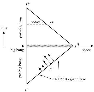
Of particular interest here are the so-called News functions, simply given by
| (3.12) |
and the “Bondi mass” given by:
| (3.13) |
The Bondi mass and the News are connected by the energy–momentum conservation equation, which tells us that the advanced-time derivative of is positive-semidefinite, and related to incoming energy fluxes controlled by the News:
| (3.14) |
The physical meaning of is that it represents the energy brought into the system (by massless sources) by advanced time . In the same spirit, one can define the Bondi mass at future null infinity . It represents the energy still present in the system at retarded time . If only massless sources are present, the so-called ADM mass is given by
| (3.15) |
while , and represents the mass that has not been radiated away even after waiting an infinite time, i.e. the mass that underwent gravitational collapse [165]. Collapse (resp. no-collapse) criteria thus aim at establishing under which initial conditions one expects to find (resp. ).
Since, as we shall see in the particular case of spherical and planar symmetry, collapse criteria i) do not involve any particularly large number, and ii) do not contain any intrinsic scale, but just dimensionless ratios of various classical scales, we expect:
-
•
Gravitational collapse to be quite a generic phenomenon.
-
•
Nothing to be there to fix either the size of the horizon or the value of at the onset of collapse.
Generically, randomly, chaotically, some regions of space at some moment in time will undergo gravitational collapse and will form horizons and singularities therein. When this is translated into the S-frame, regions of space-time within the horizon actually undergo a period of inflation in which the initial values of both the Hubble parameter and are left arbitrary. In Subsection 3.6 we shall see that such an arbitrariness provides an answer to the fine-tuning allegations that have been moved [589, 395] to the pre-big bang scenario. Before dealing with that issue, however, we shall discuss in the following two subsections cases endowed with special isometries, for which much more is known than for the general case.
3.4 The case of spherical and planar symmetry
In the spherically symmetric case, many authors have studied the problem of gravitational collapse of a minimally coupled scalar field, both numerically and analytically. In the former case we should recall the existence of well-known results [162] pointing at mysterious universalities near critical collapse (i.e. at the borderline situation in which the collapse criteria are just barely met). In this case, a very small black hole forms. This is not the case we are really interested in, for the reasons we just explained. We shall thus turn, instead, to what happens when the collapse criteria are largely fulfilled. For this we make use of the classical results presented in [164, 165, 166, 167].
In the case of spherical symmetry there are no gravitational waves, so that null wave data consist of just an angle-independent, asymptotic dilatonic waveform , with the associated scalar News . A convenient system of coordinates is the double null system , such that
| (3.16) |
where . The field equations are conveniently re-expressed in terms of the three functions , and , where the local mass function is defined by:
| (3.17) |
One then gets the following set of evolution equations for , and :
| (3.18) | |||
| (3.19) |
The quantity
| (3.20) |
plays a crucial rôle in the problem. If stays everywhere below 1, the field configuration will not collapse but will finally disperse at infinity as outgoing waves. By contrast, if the mass ratio can reach anywhere the value 1, this signals the formation of an apparent horizon (a closed trapped surface), whose location is indeed defined by the equation . The above statements are substantiated by some rigorous inequalities [167], stating that:
| (3.21) |
Thus, in weak-field regions (), we have , while, as , we have , meaning that the outgoing radial null rays (“photons”) emitted by the sphere become convergent, instead of having their usual behaviour. This is nothing but the signature of a closed trapped surface.
The emergence of a closed trapped surface implies the existence of a future singular boundary of space-time where a curvature singularity occurs [372, 166]. Furthermore, the behaviour of various fields near the singularity is just that of a quasi-homogeneous phase of dilaton-driven inflation as described by Eqs. (3.1). This highly non-trivial result strongly supports the idea that pre-big bang inflation in the S-frame is the counterpart of gravitational collapse in the E-frame.
Reference [166] gives the following sufficient criterion on the strength of characteristic data, considered at some finite retarded time
| (3.22) |
where and define two spheres, such that and , , is the width of the “annular” region between the two spheres, and is the mass “contained” between the two spheres, i.e. more precisely the energy flux through the outgoing null cone const, between and . Note the absence of any intrinsic scale (in particular of any short-distance cut-off) in the above criterion. The theorem proved in [166] is not exhausted in the above statement. It contains various bounds as well, in particular: i) an upper bound on the retarded time at which the closed trapped surgace (i.e. a horizon) is formed, ii) a lower bound on the mass, i.e. on the radius of the collapsing region.
The latter quantity is very important for the discussion of the previous subsection since it gives, in the equivalent S-frame problem, an upper limit on the Hubble parameter at the beginning of the phase of inflation. Such an upper limit depends only on the size of the advanced-time interval satisfying the collapse criterion; since the latter is determined by the scale-invariant condition (3.22), the initial scale of inflation will be classically undetermined.
The above criterion is rigorous, but probably too conservative. It also has the shortcoming that it cannot be used directly on , since on . In Ref. [130] a less rigorous (or less general) but simpler criterion, directly expressible in terms of the News (i.e. on ), was proposed on the basis of a perturbative study. It has the following attractive form:
| (3.23) |
where:
| (3.24) |
Thus denotes the “variance” of the function over the interval , i.e. the average squared deviation from its mean value.
According to this criterion the largest interval satisfying (3.23) determines the size of the collapsing region and thus, through the collapse inflation connection, the initial value of the Hubble parameter. It would be interesting to confirm the validity of the above criterion, and to determine more precisely the value of the constant appearing on its r.h.s., through more analytic or numerical work. This problem has been studied by two perturbative numerical analyses [469, 159] and also, more recently, by a numerical approach that takes into account the full non-linear evolution [461], and stresses the possible role of non-linearities in triggering the collapse of a long train of low-amplitude waves, even though the criterion (3.23) would suggest that they remain perturbative.
Let us discuss now another toy model example of gravitational collapse, that of the collision of plane waves, following closely Refs. [246] and [102]. The advantage of this case is that it can often be solved analytically, thereby providing a useful laboratory for investigating properties that we would like to be shared by more realistic situations (see some comments at the end of this subsection). For this reason we shall treat this example in considerable detail.
In order to include eventually the NS-NS two-form, we will start from the low-energy effective action in a form that already exhibits the non-compact symmetry expected from the Abelian isometries of the problem111In this subsection, for simplicity, we have denoted by what in the rest of the report would be .. This is achieved by working with a “reduced action” living in the non-trivial (two-dimensional) subspace spanned by time and by the common direction of propagation of the two waves. Following [470] we write:
| (3.25) |
Here the metric is taken to be block-diagonal, with blocks and (the Roman indices () span the transverse directions, while the Greek indices take the values 0 and 1). We arranged the components in a -dimensional matrix and the non-vanishing components in another matrix . is then the usual -dimensional matrix containing and (see Eq. (2.55)), while is the corresponding shifted dilaton (see Subsection 1.4). The reduced action (3.25) is manifestly invariant under the global transformations (2.62).
The corresponding equations of motion are written most conveniently by going to the conformal gauge for the 2-metric, , and by working with “light-cone” coordinates, . They take the explicitly -invariant form
| (3.26) | |||
| (3.27) | |||
| (3.28) |
The two colliding waves are defined as having their fronts at and , and thus to collide at (i.e. at ). The two waves are not assumed to be impulsive, i.e. their energy density can have any (finite) support at positive and , respectively.
Space-time is naturally divided in four regions: Region I, defined by , is the space-time in front of the waves, before any interaction takes place. It is trivial Minkowski space-time with and a constant perturbative dilaton (). It will be convenient to fix the constant in the definition of so that, in region I, . Region II, defined by , , represents the wave coming from the left before the collision. Metric and dilaton depend only on :
| (3.29) |
and we can consistently set . Region III can be similarly described up to interchange of and . Note that we have not assumed any special shape for , so that our results, so far, hold irrespectively of the polarization of the waves. Finally, in region IV (, ), i.e. in the interaction region, we write
| (3.30) |
and , , and are all functions of both and . Of course, the metric must be continuous along with its derivative on the boundary lines between the four regions. The same must be true for the dilaton and the antisymmetric field .
Let us begin by solving the equations in region II. The only non-trivial equation is (3.27), which (dropping the subscripts II) reads
| (3.31) |
where the dot indicates the derivative with respect to . It is now useful to change variables from to , with
| (3.32) |
After some algebra we can rewrite (3.31) as:
| (3.33) |
where is the traceless part of , and the prime denotes the derivative with respect to .
It can easily be shown that all terms on the r.h.s. of Eq. (3.33) are negative-definite. Hence, for any non trivial wave, , which is constant and identically equal to 1 in region I, must acquire a non-vanishing, negative, and never increasing derivative in region II. Thus, must vanish at some finite . Returning now to the coordinate , we see that, if the dilaton is bounded (a necessary assumption if we want to use the tree-level effective action), there exists a finite where vanishes. Correspondingly, also vanishes, and the metric of the transverse space will collapse to zero proper volume, thereby producing a (coordinate) singularity. The same arguments can be repeated in region III, where has to vanish at some finite , with . These conclusions generalize a well-known result in general relativity [577, 631] to any and to non trivial antisymmetric fields, .
Let us finally analyse region IV (where the interaction between the two waves occurs) dropping, for simplicity, the subscript IV from all functions. We begin by using Eq. (3.26), which tells us that is the sum of a function of and a function of . The unique function of this type that matches the boundary conditions with region I is
| (3.34) |
We see that must vanish on a hypersurface that joins the coordinate singularities in regions II and III and is contained in the region , within region IV.
Let us now introduce two new sets of coordinates that simplify the analysis in region IV. One set is of the light-cone type:
| (3.35) |
while the second set is of the kind:
| (3.36) | |||
| (3.37) |
Note that the coordinates run from to in region IV, with their sum always positive except on the singular boundary where . Going from the original coordinates to either of the new sets changes only the conformal factor of the 2-metric. We may thus write:
| (3.38) |
while the shifted dilaton is simply
| (3.39) |
Let us discuss in some detail the case of and parallel polarized waves following [246]. In each region, we take a diagonal with , where and goes to at in region II, and at in region III. In the new coordinates, Eq. (3.26) becomes trivial, while the equations for the and are decoupled and can be solved separately. They are also formally the same, so the solutions have the same structure [577]:
| (3.40) |
where are Legendre functions written in standard notation, and the commas denote partial derivatives. The same expression holds for , with the obvious replacements. At this point can easily be recovered once and are known.
We see that and the are singular on the hypersurface . So, in a very general way, we find that the collision of two plane waves leads to a (curvature) singularity in the space-time, whatever the number of dimensions. Although we do not have, at the moment, such an explicit solution for the general case, the discussion given in the previous section makes us believe that a curvature singularity will always emerge along the hypersurface .
For the solutions (3.40), the asymptotic behaviour for is easily found by taking the large-argument limit of the Legendre function [577] (see also [631]):
| (3.41) |
The coefficients multiplying the logarithm are functions of , whose range, on the singular surface, goes from to . One easily finds
| (3.42) | |||||
| (3.43) |
with given by the same expression as , but with replaced by . The sum of the must be zero according to the definition of the .
The asymptotic form of the metric is
| (3.44) |
while
| (3.45) |
Going over to cosmic time gives the metric in Kasner form with exponents
| (3.46) |
The following relations are immediately verified:
| (3.47) |
The behaviour of the fields near the singularity is thus of Kasner type, modified, as usual, by the presence of the dilaton. Note that, at the two tips of the singularity, and diverge in such a way that the Kasner exponents near the tips are simply , . This corresponds to a (contracting) Milne-like metric, which, being non-singular, nicely matches the non-singular behaviour in regions II and III. Away from these two points, and can take any value: it is easy to verify that the whole Kasner sphere can be covered by appropriately choosing the initial data.
It may be interesting to note that, in such a context, it is possible to estimate the entropy generated by the non-linear interaction of the incoming waves, before the Universe enters the phase of inflation, during the intermediate phase dominated by both the velocity and spatial gradients [247]. The total produced entropy is of the order of the product of the focal lengths of the two incoming waves (in Planck units), and satisfies the entropy bounds that will be discussed in Section 8.4.
Let us finally perform boosts on our solutions, in order to introduce a non-trivial field. We will refer to [102] for a full discussion and only summarize here the final result. Cosmologies with non-trivial that can be obtained, by an transformation, from a metric having Kasner behaviour near the singularity, generally contract in all dimensions. In even dimensions, at least one inflates when the original metric has just one inflating or just one contracting dimension. In odd dimensions, if the transformation has and we start from a full inflating metric or from a metric with one inflating dimension, then we are left with one inflating dimension. If , then one dimension inflates when we start from a full contracting metric or from a metric having just one contracting dimension. We should also recall that none of the transformations affects the component of the metric, which, therefore, can either inflate or contract.
How do these results generalize to more realistic situations such as the head-on collision of two plane-fronted waves, with a transverse profile that extends only over a finite range? Unfortunately such cases cannot be dealt with analytically, and numerical results are not available either, as far as we know. There have been claims [631], however, that black holes (and singularities therein) are inevitably formed, provided certain conditions are met.
Consider, an an example, two identical waves of transverse size , moving head on against each other, and carrying, in the centre-of-mass frame, energy density (per unit area) . The conjecture [631] is that a black hole of mass will form, provided
| (3.48) |
where is a number .
This conjecture appears to be confirmed by applying a recently proposed method [229] for determining when black holes are formed in point-like particle collisions at finite impact parameter. A simple extension of that method [419] to two finite-size massless waves shows that Eq. (3.48) is indeed a good criterion for black-hole formation with .
3.5 Adding -forms and BKL chaotic behaviour
We have already mentioned that adding a NS-NS two-form to the background strongly reduces the parameter space available for inflating the Universe (in string units). However, very generally, a smooth Kasner-like behaviour is still generically valid near the singularity. Spatial gradients become small with respect to time derivatives, and solutions become velocity-dominated, thereby solving, at least in principle, the flatness/homogeneity problems.
This result appears to be in contrast with what is known to happen in a standard general relativity context. Indeed, Belinskii, Khalatnikov and Lifshitz (BKL) postulated a long time ago [77] that the approach to a big crunch singularity (the time-reversal of our situation) is typically chaotic, in contrast with the naive expectation that, near the singularity, kinetic terms should dominate over spatial gradients since , for a scale factor going to zero with a small power of . This would certainly be true for an isotropic situation. However, because of the constraints on the exponents of the (general relativistic) Kasner solution,
| (3.49) |
the only non-trivial vacuum cosmologies are anisotropic.
As a consequence, there are gradient terms that are subdominant and others that, instead, grow faster than the extrinsic curvature itself (the expansion contribution to curvature), and start dominating at some point. When this happens the Kasner exponents suddenly change and a new Kasner epoch starts, until another spatial gradient dominates …, and so on indefinitely. One can visualize this behaviour as the motion of a particle in a billiard, where the Kasner-like phases are the straight motions while the sudden changes in the Kasner exponents correspond to reflections. Unless the “billiard” in question is particularly simple, a chaotic behaviour then follows. This phenomenon goes under the name of BKL oscillations.
It was known for some time that BKL oscillations occur in general relativity for any . However, the phenomenon was known to disappear if a massless, minimally coupled scalar field is added. The dilaton of string cosmology is just such a field, and therefore BKL oscillations do not appear in gravidilaton string cosmology, as explicitly shown in [59]. One way to see this is to realize that, in the presence of a dilaton, an isotropic solution is perfectly allowed, and therefore all spatial gradients can be kept under control. Thus, possibly after a small number of oscillations, the Kasner exponents end up in a region (close to the isotropic point) where no more oscillations occur until the singularity.
Adding the NS-NS two-form does not appear to change the situation with respect to BKL oscillations, as shown in many of the examples of inhomogeneous string cosmology discussed in Subsection 3.1. The same is true in the presence of various kinds of axion fields (see e.g. the case of the Type IIB string cosmology discussed in [249]), or in the context of the gravidilaton–axion–Maxwell system giving rise to inhomogeneous Gowdy-type solutions [501, 630]. On the basis of these examples it was believed for some time that BKL oscillations were the exception, rather than the rule, for string cosmology.
The surprise came when it was pointed out [191, 192] that BKL oscillations reappear generically if all the massless bosonic background fields of superstring theory (or M-theory) are turned on. Note that, even under the assumption of asymptotic past triviality, there is no reason to artificially put to zero any of these massless backgrounds. According to APT, the generic initial state should be an arbitrary superposition of weakly interacting, low-frequency waves of all kinds. Setting arbitrarily to zero some of them would amount to fine-tuning the initial state, and could even be unstable under quantum effects.
The emergence of chaos discovered in [191, 192] could have been anticipated, since we can view the gravidilaton system in as coming from dimensional reduction of a pure gravity theory in more dimensions. Upon dimensional reduction, the higher dimensional graviton generates both the dilaton and additional gauge fields. The electric and/or magnetic components of these fields, unless artificially turned off, will grow and cause BKL behaviour. Let us now go in some length into this matter, nevertheless referring to the original articles for full details.
The starting point is the low-energy tree-level bosonic action of a generic string theory (or of M-theory) which, in the Einstein frame, can be written in the form:
| (3.50) |
where the index labels the various -forms that are present in a given superstring model, and are numerically coefficients. There are actually possible additional terms, e.g. Chern-Simons terms, but these are not relevant to this discussion. One then assumes the inhomogeneous-Kasner ansatz of Subsection 3.1, rewritten in the Einstein frame as:
| (3.51) |
In order to check whether such a non-chaotic, non-oscillatory ansatz is an asymptotic solution one has to check whether all neglected terms remain parametrically small as . Several terms are possibly dangerous. Dilaton gradients are always harmless, but metric gradients are “down” with respect to the time-derivative terms by a factor , where is the following combination of Kasner exponents, . In order for these terms to be negligible, it is necessary that all be positive. Furthermore, the equations of motion for the various forms turn out to imply the constancy of both the “magnetic” components, , and of the “electric” components, , of the field strength . When such a result is inserted back in the complete equations of motion one finds further constraints on the Kasner exponents and on the “dilaton couplings” , which need to be satisfied in order for the solution (3.51) to hold.
The explicit analysis of [191, 192] shows that in any known superstring theory, as well as in supergravity (the low-energy limit of M-theory), the couplings are just what is needed to reduce the parameter space for the validity of (3.51) to a set of zero measure. The generic case is instead chaotic, and can be described in terms of motion on a billiard in a 9-dimensional hyperbolic space [194]. The reflection rules in the billiard form a group that turns out to be the Weyl group of the hyperbolic Kac–Moody algebras of or , depending on the particular superstring theory under consideration. Similar groups were also found to emerge in the case of Kaluza–Klein compactification of pure gravity in [195]. The Weyl group is now related to the Kac–Moody algebra , and the disappearance of chaos for gets related to the fact that these algebras are hyperbolic only for .
Let us finally mention a connection between the BKL chaotic behaviour and the peculiar features of some homogeneous string cosmology models, in particular those with a non-trivial antisymmetric field . We have already seen that the presence of such a backgound tends to reduce drastically (if not completely) the phase space left for inflationary pre-big bang behaviour. In Ref. [193] it was shown that this can be understood again as motion in a billiard. Whenever the initial Kasner exponents are such as to give inflation, some walls are hit a certain (finite) number of times until the ensuing reflections bring the S-frame Kasner exponents to be positive, thereby stopping the inflationary behaviour and turning it into a contraction.
From the physical viewpoint the implications of all these results are not so obvious, also because the conditions for BKL behaviour are just met at the tree level and to lowest order in . It is possible that the inclusion of either or loop corrections will bring the oscillations to a stop (after a relatively small number of them [191, 192]). It is not clear, however, which kind of string-scale-curvature hypersurface will be generated by the whole process. It is unlikely that it will be very simple and homogeneous, but it is not obvious that it will not contain isotropic and homogeneous enough patches for our Universe to emerge from.
3.6 Is pre-big bang cosmology fine-tuned?
The two arbitrary parameters discussed in the previous subsection are very important, since they determine the range of validity of our description. In fact, since both curvature and coupling increase during the initial phase of dilaton-driven inflation, the low-energy and/or tree-level description is bound to break down at some point. The smaller the initial Hubble parameter (i.e. the larger the initial horizon size) and the smaller the initial coupling, the longer we can follow the phase of low-energy inflation through the effective action equations, and the larger the number of reliable e-folds we shall gain.
This does answer, in our opinion, the objections raised [589] to the pre-big bang scenario according to which it is fine-tuned. The situation here actually resembles that of chaotic inflation [440]. Given some generic (though APT) initial data, we should ask which is the distribution of sizes of the collapsing regions and of couplings therein. Then, only the “tails” of these distributions, i.e. those corresponding to sufficiently large and sufficiently weakly coupled regions will produce Universes like ours, the rest will not. The question of how likely a “good” big bang is to take place is not very well posed and can be greatly affected by anthropic considerations [130]. Furthermore, asking for a long enough period of low-energy inflation amounts to setting upper limits on two arbitrary moduli of the classical solutions.
Figure 3.2 is a -dimensional sketch of a possible pre-big bang Universe: an original “sea” of dilatonic and gravity waves leads to collapsing regions of different initial size, possibly to a scale-invariant distribution of them. Each one of these collapses is reinterpreted, in the S-frame, as the process by which a baby Universe is born after a period of pre-big bang inflationary “pregnancy”, the size of each baby Universe being determined by the duration of the corresponding pregnancy, i.e. by the initial size of (and coupling in) the corresponding collapsing region. By using, in particular, the result of Eq. (2.110) one finds that, in , regions initially larger than (namely, larger than cm if cm) can generate Universes like ours, while smaller ones cannot.
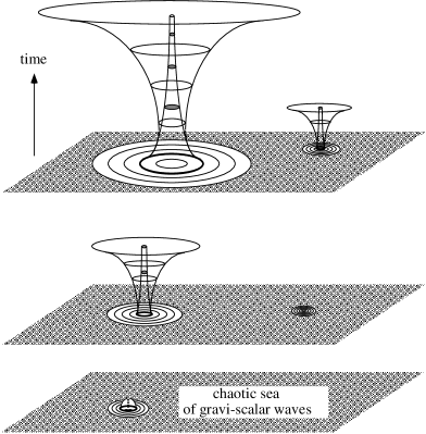
A basic difference between the large numbers needed in (non-inflationary) FRW cosmology and the large numbers needed in pre-big bang cosmology, should be stressed. In the former, the ratio of two classical scales, e.g. of total curvature to its spatial component, which is expected to be , has to be taken as large as . In the latter, the above ratio is initially in the collapsing/inflating region, and ends up being very large in that same region, thanks to the inflation. However, the (common) order of magnitude of these two classical quantities is a free parameter, and it is taken to be much larger than the classically irrelevant quantum scale. Indeed, the smallness of quantum corrections (which would introduce a scale in the problem) was explicitly checked in [344].
An example of what we have just said is the case of the collision of two finite-front plane waves. It is clear from Eq. (3.48) that all that matters is the ratio of two geometrical classical quantities, the transverse size and the focal distance . Neither the Planck nor the string lengths appear in the collapse criterion. Even the appearance of the Newton constant in (3.48) is somewhat misleading: as always in the context of classical general relativity, the Newton constant can be removed by a convenient choice of units of energy, and then everything reduces to geometrical quantities.
We can visualize analogies and differences between standard and pre-big bang inflation by looking again at the two cases of Figs. 1.2 and 1.3. The common feature in the two pictures is that the fixed comoving scale corresponding to the present horizon was “inside the horizon” for some time during inflation, possibly very deeply inside at its onset. The difference between the two scenarios is just in the behaviour of the Hubble radius during inflation: increasing in standard inflation, decreasing in string cosmology. Thus, while standard inflation is still facing the initial-singularity question, and needs a non-adiabatic phenomenon to reheat the Universe (a kind of small bang), pre-big bang cosmology faces the singularity problem later, combining it with the exit and heating problems (see Section 8).
A much more relevant objection to this approach to initial conditions is the one raised in [191, 193]. If the initial conditions are to be really generic (although satisfying APT), then all massless waves should be allowed. Already with antisymmetric tensor waves the phase of dilaton-driven inflation is becoming non-generic, while, when all massless forms are included, BKL behaviour seems to be the generic situation, at least before strong curvature and/or strong coupling is reached. Understanding the fate of such evolutions calls for a deeper understanding of how string effects may resolve the singularity problem (to be discussed in Section 8).
4 Amplification of quantum fluctuations
If we accept, at least as a working hypothesis, the idea that the pre-big bang scenario illustrated in the previous sections might represent a possible candidate for a self-consistent representation of the primordial cosmological evolution, we are eventually led to the following fundamental questions: Is it possible to find phenomenological effects that can differentiate the pre-big bang scenario from other, more conventional inflationary scenarios, and Are such differences observable today, at least in principle?
In order to answer this question we may note that the accelerated evolution of the Universe is a process accompanied by the production of an enormous amount of radiation. Almost all types of fields are excited, and particles are copiously produced, with an efficiency that reaches its maximum during the explosive “big bang” regime. By studying the properties of the relic cosmic backgrounds we may obtain information about the very early state of the Universe, just as by studying the quantum numbers of the particles produced in a decay process we can get information on the quantum state of the system before the decay.
From the various mechanisms of radiation production, active on a cosmological scale, we will consider here the parametric amplification of the quantum fluctuations of the vacuum, because it is typical of all backgrounds with accelerated kinematics, and it is effective in all inflationary scenarios. It thus represents a good “indicator” of the dynamics of the early Universe [350, 351, 357] and an appropriate starting point to discriminate among different inflationary models.
Although in this section we will mainly concentrate on the study of the metric fluctuations, our discussion can be easily applied to the evolution of the fluctuations of any background field. The convenient formalism to be adopted for the study of this process is the theory of cosmological perturbations (see [493, 434] for two excellent and comprehensive reviews), which provides a straightforward and (in principle) simple approach to the problem. According to this approach, given a set of background field equations
| (4.1) |
the standard procedure is to perturb (to first order) the metric and the matter sources:
| (4.2) |
expanding around a given cosmological solution. By using the unperturbed equations for the bakground fields, , one easily obtains a system of linear equations describing the evolution of the first-order fluctuations of the metric and of the matter fields,
| (4.3) |
and can then discuss, on the basis of these equations, the amount of radiation production.
This perturbative approach is the same for all cosmological scenarios. There are two important differences, however, that characterize pre-big bang models with respect to other inflationary models.
The first difference concerns the higher-dimensional and scalar-tensor (i.e. gravidilaton) nature of the string cosmology backgrounds. As a consequence, there are possible contributions to the amplification of the fluctuations not only from the inflation of the three-dimensional space, but also from the dynamics of the extra-dimensions [265, 26, 208, 297], and from the time evolution of the coupling constants (i.e. of the dilaton), as first pointed out in [300]. The amplification of the perturbations thus becomes possible also for fields conformally coupled to the 3-dimensional metric, unlike in the standard cosmological scenario [91].
The second difference concerns the growing character of the background curvature and of the couplings. In such a background the quantum fluctuations start evolving from an asymptotically flat, zero-coupling state, so that they can be naturally normalized to an initial vacuum fluctuation spectrum. After the amplification their final configuration thus corresponds to a “squeezed vacuum” state [355, 356, 352], and not to a “squeezed-thermal vacuum” [305], or to other, more complicated states. In addition, since the final energy distribution tends to follow (in frequency) the behaviour (in time) of the curvature scale, one typically obtains in such a context a growing (or “blue”) spectrum [571, 4, 350, 13, 549, 357]. As a consequence, the peak amplitude of the produced radiation may be high enough to support a picture in which all the radiation filling our present Universe was directly produced from the quantum fluctuations of the vacuum [602, 276]. This effect may facilitate the detection of a cosmic background of relic gravitational waves [296, 273], as will be discussed in Section 5, but it complicates the generation of a scale-invariant spectrum of curvature perturbations, eventually producing the observed CMB anisotropy (see Section 7).
A further consequence of the growth of the curvature scale, however, is that the comoving amplitude of the perturbations may even grow outside the horizon, instead of being frozen as in standard inflationary models. This effect, implicitly contained in the earlier pioneering studies of cosmological perturbations [571], was first explicitly pointed out in [3], and only later independently rediscovered in a string cosmology context [321] and in the context of scalar-tensor gravity [65]. Such a growth of the amplitude may require an appropriate and non-conventional choice of the gauge [116] in order to restore the validity of the linear approximation, and to allow the application of the standard perturbative formalism.
In the following subsections we will discuss in some detail the above effects, typical of the evolution of perturbations in the context of the pre-big bang scenario.
4.1 “Frame” independence
The computation of the spectrum according to the theory of cosmological perturbations [493] requires a series of formal steps, the first of which is the choice of the “frame”, i.e. of the basic set of fields (metric included) used to parametrize the action. Any theory is in general characterized by a preferred set of fields, but one might wonder what happens when there are more than one preferred choices (this is a typical situation of all scalar-tensor models of gravity, as in the case of the gravidilaton string effective action).
In string theory there is a preferred frame (the so-called S-frame), in which the coupling to a constant dilaton is unambiguously fixed (at the tree level) for all fields and to all orders in the higher-derivative expansion. Also, the metric of this frame is the one to which fundamental strings are minimally coupled [552, 315] (in other words, the world-paths of strings freely evolving in a curved background are geodesic surfaces of this metric). In the S-frame, and in dimensions, the gravidilaton effective action takes the form
| (4.4) |
(for the sake of generality we have included here the Brans–Dicke coefficient , which in our context could represent a dilaton self-coupling possibly arising from higher-loop corrections [347]; in particular, for the lowest-order string effective action).
For any , however, this action can always be rewritten in the (more conventional) E-frame, in which the graviton and dilaton kinetic terms are diagonalized in the standard canonical form, and the dilaton is minimally coupled to the metric. Consider, in fact, the field redefinition performed with the help of a new scalar variable :
| (4.5) |
By expressing the scalar curvature in terms of [616, 576], the action (4.4) becomes
| (4.6) |
where the tilde denotes geometrical quantities computed with respect to . By setting ( const, ):
| (4.7) |
and neglecting a total derivative, we are led eventually to the E-frame action of general relativity for the new variables :
| (4.8) |
Please note the “right” canonical coefficient in front of the dilaton kinetic term (we remember that we are using the signature ) and the possible change of sign from the S-frame action (4.4) (where , to lowest order). The E-frame is thus preferred for performing canonical quantization, for identifying the particle content of the theory, and for defining the effective low-energy masses and couplings (see also Section 6).
However, the field equations for , obtained by varying the action (4.4), are different from the equations for , obtained by varying the action (4.8). As a consequence, also the perturbation equations (4.3), in the S-frame, are different from the E-frame perturbation equations, and one might wonder which is the “right” frame to be used, when computing cosmological effects to be compared with present observations.
This is a false problem, however, because the (final) observable variables, such as the spectral amplitude, the spectral energy density (see Subsection 4.4), are exactly the same in both frames [321] (an obvious consequence of the fact that physical measurable quantities cannot be changed by field redefinitions such as the transformation (4.5); see also [20] for a recent discussion of the equivalence between the String and Einstein frames). The formal reason of this frame-independence is that the perturbation equations are indeed different in the two frames, but the classical solutions around which the expansion is performed are also different, and the two differences exactly compensate each other. This result can be generally proved by perturbing the action, better than the equations of motion (see Section 4.3). It is instructive, however, to give also a particular example, as will be done here by considering tensor metric perturbations propagating in a ()-dimensional external background.
We will start the computation in the S-frame, where the background equations obtained from the action (4.4) can be written explicitly as
| (4.9) |
We shall consider the transverse, traceless part of the metric perturbations,
| (4.10) |
propagating in a higher-dimensional, spatially flat, factorizable background with “external” and “internal” dimensions, with scale factors and , respectively. Also, we shall assume that the translations along the internal dimensions are isometries of the full, perturbed metric (see [328] for a more general situation in which also the internal gradients of the fluctuations are non-zero, and see the comment after Eq. (4.25) for backgrounds with non-factorizable geometry). The fluctuations of the external space are then conveniently described in the synchronous gauge [426], where (; ):
| (4.11) |
In this gauge
| (4.12) |
to first order in , the perturbation of the dilaton equation is found to be trivially satisfied, and there are no contributions from the terms inside the square brackets in (4.9). The perturbation equations are thus (remarkably) -independent [300]:
| (4.13) |
For , they are trivially satisfied. The components of the Ricci tensor, on the other hand, lead to the higher-dimensional covariant d’Alembert operator [297, 209, 300]
| (4.14) |
where and the indices of are raised and lowered with the unperturbed metric. Using the identities (see also [278])
| (4.15) |
we are finally led to the S-frame tensor perturbation equation [300]
| (4.16) |
In terms of the conformal time coordinate , such that , this wave equation can also be rewritten (for each polarization mode ) as follows,
| (4.17) |
Let us now repeat the computation in the E-frame, where the background equations following from the action (4.8) can be written as
| (4.18) |
Perturbing to first order, and using Eqs. (4.10):
| (4.19) |
(the perturbation of the scalar Klein–Gordon equation is trivially satisfied). In the synchronous gauge, we can still apply Eq. (4.14) (for the “tilded” variables), and we are finally led to the E-frame perturbation equation
| (4.20) |
In conformal time, and for each polarization component ,
| (4.21) |
This last equation seems to be different from the S-frame equation (4.17). We have to recall, however, that the conformal time is the same in both frames, (see Section 2.4), and that, according to Eq. (4.5),
| (4.22) |
We thus have the same equation for and , the same solution and, as a consequence, the same spectrum when the solution is expanded in Fourier modes.
In other words, the observable results of the perturbative analysis are “frame-independent” and, when computing the spectrum, we are allowed to use the frame that is most convenient for practical purposes.
4.2 Choice of the “gauge” for scalar perturbations
Within each frame, we have a possible additional ambiguity due to the choice of the gauge, i.e. the choice of the parametrization of the given metric manifold. The step corresponding to this choice is more delicate than the choice of the frame: in spite of the fact that the final observable spectrum has to be certainly independent of the given coordinate system, the perturbative analysis is, on the contrary, “gauge-dependent”. It is possible, for instance, that a linearized description of the perturbations is valid in a given system of coordinates, and yet that the linear approximation is broken in a different system. This problem obviously disappears in the context of a fully covariant and gauge-invariant (to all orders) description of perturbations [235, 113]. For the perturbative approach usually adopted in a cosmological context [493], however, gauge invariance holds in the linear approximation only, and breaks down at higher orders.
An important example of this effect is provided, in string cosmology, by the time evolution of the scalar (metric and dilaton) perturbations. We will discuss this effect in the E-frame (dropping the “tilde”, for simplicity), starting from the unperturbed equations (4.18), and using, as in the previous subsection, a homogeneous, Bianchi-I-type, higher-dimensional background, with factorized structure:
| (4.23) |
We shall consider, in particular, the exact background solution parametrized by
| (4.24) |
and corresponding to the conformal-time parametrization of the vacuum solution already introduced in Eq. (2.114). For , , this unperturbed solution describes a phase of accelerated evolution, growing curvature and growing dilaton, in which the horizon expands more slowly (to be more precise, shrinks faster) than the scale factor. It is thus a good background candidate to amplify metric fluctuations. In the S-frame it describes a phase of superinflation and dynamical dimensional reduction, in which dimensions are expanding and dimensions are contracting, with scale factors related by the duality transformation .
Let us perturb the metric and the dilaton around this solution, by using the isometries of the factorizable geometry (4.23) and assuming that all dynamical variables depend only on the “external” coordinates , (so that the translations along the internal dimensions are also isometries of the full, perturbed background) [301]. In this case, modes with different rotational transformation properties are decoupled, and the scalar component of the background perturbations can be written in general as [493, 301]:
| (4.25) |
where all variables depend only on and . It should be noted that this approach is appropriate to the standard Kaluza–Klein scenario, but it cannot be applied to non-factorized geometrical structures such as those appearing in the context of the Randall–Sundrum scenario [531]. In this last case, the study of scalar metric and dilaton fluctuations (see for instance [100, 337]) requires a more general metric decomposition [597]. In this report, however, we will restrict our discussion to the perturbations of higher-dimensional Kaluza–Klein backgrounds of the standard, factorizable type.
In our case, it is important to stress that the six functions are not invariant under local infinitesimal transformations of coordinates,
| (4.26) |
However, if we consider infinitesimal coordinate transformations depending on two scalar parameters abd ,
| (4.27) |
and thus preserving the scalar character of the perturbations (in other words, coordinate transformations that do not add vector or tensor components to the perturbed metric), then the scalar variables transform as
| (4.28) |
and it is always possible to define a set of variables that are gauge-invariant, in the linear approximation. For instance [301]:
| (4.29) |
The first two variables (also called Bardeen potentials [54, 554]) are phenomenologically important, since their spectral amplitudes , at the recombination era are directly related (via the Sachs–Wolfe effect) to the large-scale CMB anisotropy , currently observed by astrophysical experiments (see Section 7).
A natural and convenient choice of the gauge is thus the so-called longitudinal (or conformally Newtonian) gauge, in which , and the perturbed metric depends directly on the Bardeen potentials, according to Eqs. (4.29). In this gauge the coordinates are totally fixed because, according to the variation of the metric under the transformation (4.28), the choice completely fixes and , and leaves no residual degrees of freedom.
In this gauge we can now write explicitly the set of perturbed field equations
| (4.30) |
obtained from the unperturbed Einstein equations (4.18). From the () component of the perturbation equations we obtain a useful relation between three perturbation variables,
| (4.31) |
The () components give a constraint, while the () and () components of the perturbed Einstein equations, combined with the () component, provide the following interesting system of coupled equations for the “external” and “internal” perturbations and [301, 327]:
| (4.32) |
where denotes here the usual (flat-space) d’Alembert operator.
This system can easily be diagonalized to find the (time-dependent) linear combination of and that represents the true “propagation eigenstates”. For our purpose, however, the asymptotic behaviour of the modes , can be simply obtained (modulo logarithmic corrections) by inserting into the previous system the power-law ansatz
| (4.33) |
For the background solution (4.24) one then finds that there are, in the limit, non-trivial solutions for the coefficients and only if or . This means that, asymptotically,
| (4.34) |
and the amplitude is not frozen, unlike in the standard inflationary scenario. Because of the growing mode, , the scalar perturbation amplitude blows up in the limit . Otherwise stated, at any given time there is always a low enough frequency band for which the typical fluctuations have a dimensionless amplitude much larger than [116] (see Eq. (4.75) in the next subsection). This breaks the validity of the linear approximation and is not consistent, in general, with the perturbative expansion around a homogeneous background.
This conclusion cannot be avoided, be it by moving to a different frame (as discussed in the previous subsection), or by changing the number of dimensions, since the previous result is dimensionality-independent. For a isotropic background, in particular, one finds in the longitudinal gauge , and the Fourier modes satisfy the Bessel equation
| (4.35) |
(from Eq. (4.32)). The exact solution, in the limit , has the asymptotic expansion [6]
| (4.36) |
( are integration constants), with the same growing mode as in higher dimensions.
It is important to point out, however, that such a growing mode is absent for tensor metric perturbations. If we consider the tensor perturbation equation (4.21), in the same background (4.24), we obtain indeed for each Fourier mode the Bessel equation
| (4.37) |
with the asymptotic solution
| (4.38) |
All modes tend to stay constant, asymptotically, modulo a logarithmic growth that can be easily kept under control if the phase of accelerated evolution is not infinitely extended in the high-curvature regime but is bounded, for instance, by the Planck (or string) scale (as expected).
This is a first signal that the growing mode of scalar perturbations, appearing in the longitudinal gauge, might be a pure gauge effect, i.e. an artefact of the particular choice of coordinate system. This suspicion is confirmed by the application of the “fluid flow” approach [369, 434] to the perturbations of a scalar-tensor background. In this approach, the evolution of density and curvature inhomogeneities can be described in terms of covariant scalar variables, which are gauge-invariant to all orders [113].
Let us consider, for simplicity, the isotropic case , . There are two covariant variables, and , defined in terms of the momentum density of the scalar field , of the spatial curvature , and of their derivatives. By expanding around the dilaton-driven background (4.24), which in our case reduces to
| (4.39) |
one finds for such variables, in the linear approximation, the asymptotic solution () [116]:
| (4.40) |
Such variables tend to stay constant outside the horizon, with at most a logarithmic variation (as in the tensor case), which is not dangerous. Indeed, in terms of and , the amplitude of density and curvature fluctuations can be consistently computed using the linear approximation (for all modes), and their spectral distribution (normalized to an initial vacuum spectrum, see the next subsection) turns out to be exactly the same as the tensor spectral distribution (4.38), which is bounded.
The same result, on the other hand, can also be directly obtained in the longitudinal gauge simply by neglecting the growing mode of Eq. (4.36), as noted in [322]. This suggests that it should be possible to move to a more appropriate gauge, in which the growing mode is suppressed, to restore the validity of the linear approximation.
This is exactly what happens in the off-diagonal gauge (also called “uniform-curvature” gauge [382]), defined by ,
| (4.41) |
which represents another complete choice of coordinates, with no residual degrees of freedom (just as the longitudinal gauge). In this gauge there are two variables for scalar perturbations, and , and the perturbation equations are solved, asymptotically, by
| (4.42) |
The growing mode is thus completely absent for homogeneous perturbations (since it is that contributes to the perturbed metric). The growing mode is still present in the off-diagonal part of the metric for non-homogeneous perturbations, but it is suppressed with respect to the longitudinal gauge, since , instead of . The lower is the stronger is the suppression, and this is enough for the linear approximation to be valid, as explicitly checked with a computation up to second-order corrections [116]. This off-diagonal gauge is in general useful for the study of scalar perturbations also in the context of generalized scalar-tensor models of gravity and of the higher-loop string effective action, as discussed for instance in [384].
Even better, one may choose a gauge in which . In this gauge, is related to the Bardeen potential by , according to Eq. (4.29). On the other hand, the gauge-invariant Bardeen potential evolves asymptotically (in all gauges) like the longitudinal variable , i.e. like . Since enters the metric perturbations with two spatial derivatives, it follows that, in this gauge, , which is asymptotically frozen, and sufficiently small (at small ) for the linear approximation to be valid.
To conclude this subsection, let us stress that the asymptotic growth of perturbations is a typical problem of string cosmology, with no counterpart in the standard inflationary scenario. Consider, for instance, a , conformally flat and accelerated background, which can be conveniently parametrized in the negative range of the conformal time coordinate by a generic power-law scale factor, as follows:
| (4.43) |
For ranging over the whole real axis we can represent in this way all classes of inflationary backgrounds introduced in Section 1.3, and reported in Table 1. Consider then the E-frame perturbation equation (4.21), which in this case reduces to the Bessel equation
| (4.44) |
with asymptotic solution (for ):
| (4.45) |
The amplitude tends to stay constant for , while it tends to grow for (for the growth is simply logarithmic). In the E-frame the growing mode thus appears only for a phase of accelerated contraction (see Table 1), and it is absent in the standard inflationary context where the background is always expanding (even in the E-frame).
| de Sitter | ||
|---|---|---|
| power-inflation | ||
| superinflation | ||
| accelerated contraction |
In the pre-big bang scenario, on the contrary, the comoving amplitude of metric fluctuations may be growing, in the standard gauges, even in the case of tensor perturbations. In some cases the validity of the linear approximation may be restored in an appropriate gauge, as for the scalar case discussed in this subsection. If this is impossible, the growth of perturbations is a physical effect, signalling a (quantum) instability of the given background [407, 409]. In any case, however, the energy spectrum of the perturbations can always be consistently estimated by truncating the comoving amplitude to the frozen part of the asymptotic solution [119]. This is a consequence of a duality property of the perturbation equations that will be discussed in Subsection 4.5.
4.3 Canonical variables and normalization
The linearized equations for the classical evolution of the perturbations have been obtained, in the previous subsection, by perturbing directly (to first order) the equations of motion of the background fields. The same equations, however, can also be obtained with a different approach, by expanding the action up to terms quadratic in the first-order fluctuations:
| (4.46) |
The variation of the perturbed action with respect to gives in fact a set of linearized equations, identical to Eqs. (4.3).
This second method is longer, in general, but has an advantage: the diagonalization of the quadratic perturbed action defines the “normal modes” of oscillation for the total system formed by the metric plus the matter sources. The so-called normal modes are the variables that diagonalize the kinetic part of the action and that, once quantized, satisfy canonical commutation relations [493]. They are required to normalize the initial amplitude of the perturbations to a quantum spectrum of zero-point (vacuum) fluctuations, and to study their amplification in the course of the cosmological evolution.
Let us illustrate this point starting with the case of tensor metric perturbations. The second-order action for tensor perturbations in a cosmological background was first written in [261], in the E-frame and in dimensions (see also [493, 17]). Such a result can be easily generalized to the S-frame [278] and to the ()-dimensional, Bianchi-I-type metric background used in the previous subsections, starting from the unperturbed, low-energy gravidilaton string effective action (in units ):
| (4.47) |
and considering the transverse, trace-free variable , defined by the first-order perturbation (4.10). As already discussed, the fluctuations of the -dimensional external space are conveniently described in the synchronous gauge of Eq. (4.11). In this gauge, we expand to order the controvariant components of the metric,
| (4.48) |
the volume density,
| (4.49) |
and so on for , (see [278] for the details of the explicit computation). The second-order perturbed action has then contributions from , and :
| (4.50) |
Integrating by parts, using the unperturbed equations of motion, and neglecting total derivative terms, we finally arrive at the quadratic action:
| (4.51) |
Decomposing the fluctuations of the -dimensional spatial metric into the two physical polarization modes , ,
| (4.52) |
and introducing the conformal time coordinate , we eventually obtain,for each mode, the effective scalar action
| (4.53) |
where is now a scalar variable standing for either of the polarization amplitudes , . The variation with respect to now gives exactly Eqs. (4.17), i.e. the S-frame tensor perturbation equation (the sameas was obtained by direct perturbation of the equations of motion).
The above action describes a scalar field non-minimally coupled to a time-dependent external field (also called “pump field”), represented in this case by the dilaton and by the internal and external scale factors (the so-called “moduli”). In order to impose the correct normalization to a quantum spectrum of vacuum fluctuations we need, however, the canonical variable that diagonalizes the kinetic part of the action and describes asymptotically a freely oscillating field [213, 353, 493]. In our case such a variable is defined by [300]
| (4.54) |
In fact, for each Fourier mode , we get from Eq. (4.53), after integration by parts, an effective action in which the kinetic term appears in the standard canonical form:
| (4.55) |
and which leads to the canonical evolution equation:
| (4.56) |
with an effective potential depending only on the external pump field. An accelerated background, in particular, has an effective potential that goes to zero as . We thus obtain, asymptotically, the free-field equation
| (4.57) |
and the variable can be normalized to an initial-vacuum fluctuation spectrum,
| (4.58) |
so as to satisfy canonical commutation relations . The normalization of the canonical variable automatically fixes the normalization of the metric fluctuations, .
It is important to stress that the procedure used to introduce the diagonalized action (4.55) can be exactly repeated in the E-frame. The only difference in this new frame is that there is no dilaton coupling in front of the Lagrangian density, and the pump field is simply determined by the E-frame scale factors, . But, according to the transformation rule (4.22), . The effective potential is thus the same in the two frames, the time evolution of and is the same and, as a consequence, we find the same spectrum in both frames, as anticipated in Subsection 4.1.
In the case of scalar metric perturbations, the computations are more complicated, in practice, but the procedure is exactly the same in principle. The scalar canonical variable has been computed for a isotropic background coupled to various types of sources: a perfect fluid [456, 160], one scalar field [555, 491, 572], two scalar fields [214], scalar fields [29]. Working in the E-frame (and omitting the “tilde”, for simplicity) the scalar perturbation of the gravidilaton action (4.8) can be easily performed in the longitudinal gauge, where , , . One then obtains the diagonalized second-order action [493]:
| (4.59) |
where the canonical variable is defined by
| (4.60) |
and is gauge-invariant, as can be explicitly checked by using the infinitesimal transformations (4.28).
This result can be easily generalized to the scalar fluctuations of the higher-dimensional, anisotropic background considered in the previous subsections, and parametrized as in Eq. (4.25). After the diagonalization, the higher-dimensional action for the Fourier modes of scalar perturbations can be written as [301]
| (4.61) |
(modulo a total derivative that does not contribute to the equations of motion). There are two gauge-invariant canonical variables, and , which in the longitudinal gauge () are defined by
| (4.62) |
with the generalized pump field
| (4.63) |
The definition of the canonical variable and the correct normalization of the perturbations are necessary ingredients to study the growth of the quantum fluctuations, and to determine whether they backreaction may become eventually so large as to destroy the initial homogeneity of a pre-big bang solution (see also Section 3). It is the canonical normalization, in particular, that leads to the standard relation between the amplitude of quantum fluctuations and the curvature scale of the background geometry.
In order to illustate this important point let us consider tensor perturbations in a , isotropic, E-frame metric, evolving in time aymptotically according to Eq. (4.45). The classical perturbation equation (4.44) only determines the time dependence of the fluctuations. The canonical action, however, determines not only the -dependence through the normalization of , but also the correct canonical dimensions of the fluctuations, . By inserting in fact the required dimensional factors in the (E-frame) perturbed action,
| (4.64) |
we obtain the scalar field action (4.55) with canonical dimensions by setting, for each Fourier mode,
| (4.65) |
(recall that with our conventions).
The typical fluctuation amplitude over a comoving length scale , on the other hand, is determined by the two-point correlation function
| (4.66) |
where the brackets denote either a quantum expectation value, if we work in the formalism in which the perturbations are quantized and expanded into annihilation and creation operators (see Subsection 4.4), or a macroscopic ensemble averaged over a spatial volume, if we work in the classical limit. In any case we consider real perturbations (), satisfying the isotropy condition (i.e. is a function of only) and the stochastic condition
| (4.67) |
(which is a consequence of their quantum origin). An explicit computation then gives [493, 279]
| (4.68) |
where represents the typical, dimensionless amplitude of tensor fluctuations over a comoving length scale :
| (4.69) |
The amplitude of the quantum fluctuations of the metric is now fixed by Eq. (4.65) and by the normalization of the canonical variable, Eq. (4.58). Initially, for , all fluctuations oscillate inside the horizon, and
| (4.70) |
i.e. the amplitude of a mode is proportional to its proper frequency (and then it is adiabatically decreasing, in an expanding background). In the opposite regime , where the fluctuations are well outside the horizon of an inflationary background with , we have to use the asymptotic solution (4.45), and we may distinguish three possibilities.
-
•
If , then is frozen, while the canonical variable grows adiabatically, following the growth of the pump field (see Eq. (4.45)): , where “hc” denotes the time of horizon crossing, ). The final amplitude can thus be expressed in terms of the background curvature scale at the crossing time :
(4.71) where is some reference scale (a convenient choice is the final curvature scale at the end of the inflationary phase), and is the conformal power of the scale factor. The spectral amplitude is frozen in time, and it is then clear from the above equation why pre-big bang models, characterized by a growing (in time) curvature scale (, see Table 1), are associated to a growing (in frequency) tensor perturbation spectrum.
-
•
If , then is growing according to Eq. (4.45) and, as a consequence, the spectral amplitude grows not only in frequency but also in time:
(4.72) - •
It is important to stress that the behaviour of scalar fluctuations, in the background with , is apparently very different from the tensor one, as already discussed in the previous subsection. By eliminating the dilaton fluctuation , and using the scalar perturbation equations, one finds indeed that the scalar longitudinal variable is related to the canonical variable of Eq. (4.60) by [493]:
| (4.74) |
The normalized amplitude of scalar quantum fluctuations,
| (4.75) |
is thus unbounded since, for any , we can always find a frequency band for which is arbitrarily large.
By using the correct quantum normalization, however, it is now easy to check that this difficulty disappears in the off-diagonal gauge [116], where the off-diagonal perturbation variable satisfies and the amplitude of the corresponding quantum fluctuations is controlled by
| (4.76) |
For the typical inflation scale of string cosmology, , this amplitude stays smaller than for the whole duration of the pre-big bang phase, , and for all modes with (higher-frequency modes are not amplified, see the next subsection). It should be mentioned, however, that this conclusion does not apply to classical fluctuations, whose initial amplitude is not constrained by the quantum normalization (4.58), and can be fixed to much higher values (see a recent discussion in [129]).
To conclude this subsection we note that the above procedure used to define the canonical variables can also be applied to more complicated models, and in particular to the actions including the higher-derivative corrections typical of the “stringy”, high-curvature regime [483, 141], appearing towards the end of the phase of pre-big bang evolution. To first-order in , and in the S-frame, such an action can be parametrized as [308]
| (4.77) |
where is the Gauss–Bonnet invariant (see Section 8.2 for further details). Starting with Eq. (4.77), the second-order perturbed action for each polarization mode of tensor fluctuations becomes [278], in conformal time,
| (4.78) |
where
| (4.79) |
(the inequality of the two pumping fields and , which prevents factorization, is a consequence of the breaking of the scale-factor duality symmetry, to this order in ; see [477] for an action with corrections, which preserves scale-factor duality). By setting we get the action in canonical form,
| (4.80) |
and the corresponding perturbation equation
| (4.81) |
looks the same as Eq. (4.56), with the only difference that the effective potential is now, in general, -dependent. The above equation takes into account (to first order) higher-curvatures effects on the perturbation spectrum [278], and provides the starting point for studying the evolution of tensor perturbations in the high-curvature regime typical of the pre-big bang scenario [149]. A similar approach has been developed for the study of scalar and vector fluctuations including corrections [151].
4.4 Spectral distribution of the energy density
For all types of perturbations the evolution in time of the canonical modes is described by the Schrödinger-like equation (4.56), with an effective potential that depends on the pump field, and thus on the peculiar kinematics of the given background. For all inflationary backgrounds, however, such a potential tends to vanish, asymptotically, at large positive and negative values of the conformal time.
Consider, for instance, the evolution of tensor perturbations in the E-frame: the pump field is the scale factor, , and . For a typical inflationary scenario the background is initially accelerated, parametrized by a power-law scale factor, , so that for ; at large times the background eventually evolves into the standard radiation-dominated era, , so that for . The analysis of perturbations thus reduces to a problem of scattering of the “wave function” , induced by a potential , which is asymptotically vanishing (see Fig. 4.1).
The important difference between the present problem and an ordinary scattering problem, however, is that the differential variable of Eq. (4.56) is time, not space. As a consequence, the oscillation frequencies represent energies, not momenta. With an initial normalization to a state of positive energy,
| (4.82) |
the final state is thus in general a superposition of positive and negative energy modes,
| (4.83) |
In the context of quantum field theory, it is well known that such a mixing represents a process of pair creation from the vacuum [91]. The so-called Bogoliubov coefficients parametrize the unitary transformation connecting the set of and annihilation and creation operators:
| (4.84) |
and define the expectation number of pairs produced from the vacuum in the mode :
| (4.85) |
In a second quantization language, the amplification of perturbations can thus be described as a process of particle production or, equivalently, as the evolution of the initial vacuum into a final “squeezed” vacuum state [352, 353, 355, 356],
| (4.86) |
generated by the two-mode squeezing operator [566]
| (4.87) |
Here is the so-called squeezing parameter, whose modulus and phase are related to the Bogoliubov coefficients by [566]
| (4.88) |
Itshould be noted that the squeezed-state formalism is particularly convenient for the analysis of the statistical properties of the produced radiation, and for the study of the entropy growth associated to particle production. Representing the effective decoherence of the squeezed density matrix through a suitable “coarse-graining” procedure, which accounts for the loss of information associated to (averaged) macroscopic observations, one finds indeed that the entropy growth associated to particle production, for each mode , is given by [298, 299]. In the large squeezing limit, summing over all modes, the total entropy inside a proper volume can then be estimated as
| (4.89) |
in agreement with different approaches to the same problem [107, 108], and with different definitions of quantum (von Neumann) and informatic (Shannon–Wehrl) entropy [302]. For a growing, power-law spectral distribution , typical of pre-big bang models, one obtains a constant entropy per comoving volume, , where is the maximal amplified frequency inside the given volume. This result has useful applications to the problem of the graceful exit, as will be discussed in Section 8.4.
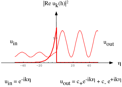
In a semiclassical language, the amplification of perturbations can be represented instead as a parametric amplification [349, 571] of the wave function , i.e. as an “antitunnelling” process [279] in which the positive frequency part of the mode (4.83) plays the role of the wave incident (from the right) on the barrier and its negative part the role of the reflected wave, while the mode (4.82) plays the role of the transmitted wave (see Fig. 4.1). The Bogoliubov coefficient , which controls the number of produced particles, can then be written as the ratio of the reflection and transmission coefficients, . In the parametric amplification regime, characterized by a large number of produced particles (), one finds , so that , and then
| (4.90) |
Hence the term antitunnelling.
Quite independently of the adopted language, the energy density of the produced particles, for each mode (summing over two polarization states), is given by
| (4.91) |
The computation of the spectral energy distribution per logarithmic interval of frequency,
| (4.92) |
thus requires the computation of the Bogoliubov coefficient . By recalling Eqs. (4.82), (4.83), this amounts to solving the perturbation equation in the limit of large positive times, with the initial normalization imposed at .
We will consider, as a simple example, a model of background characterized by two phases: an initial accelerated evolution up to the time , and a subsequent radiation-dominated evolution for :
| (4.93) |
In the first phase the canonical equation (4.56) for tensor perturbations reduces to a Bessel equation,
| (4.94) |
with general solution [6]
| (4.95) |
where are the first- and second-kind Hankel functions, of index determined by the kinematics of the background (in this case, by the time evolution of the scale factor; more generally, however, parametrizes the evolution of the pump field in conformal time). By using the large argument limit [6] for ,
| (4.96) |
we normalize the solution to a vacuum fluctuation spectrum,
| (4.97) |
In the second phase , and we have the simple oscillating solution,
| (4.98) |
The coefficients are now determined by the continuity of and at . More precisely, assuming a non-singular and continuous background, the matching would require the continuity of the perturbed metric projected on a space-like hypersurface containing , and the continuity of the extrinsic curvature of that hypersurface [386, 215]; but in many cases these conditions are equivalent to the continuity of the canonical variable , and of its first time derivative (see however [136]). Such a matching prescription might require modifications, however, in the case of bouncing backgrounds [519] evolving from contraction to expansion).
When matching the solutions (4.95), (4.98), it is convenient to distinguish the two regimes in which the comoving frequency is much higher or much lower than the frequency associated to the top of the effective potential barrier, . In the first case, , we can use the large-argument limit of the Hankel functions to find that there is no significant particle production, i.e.
| (4.99) |
Actually, is not exactly zero, but it is exponentially suppressed [13, 265] as a function of frequency, just like the quantum-mechanical reflection probability for a wave function with a total energy well above the top of a potential barrier. Such an effect is, however, negligible for the purpose of a first-approximation estimate in a cosmological context, and in any case it only affects the shape of the very high-frequency tail of the spectrum. A sharp cut-off, in that region, is a good enough approximation.
In the second case, , we can use the small-argument limit of the Hankel functions [6],
| (4.100) |
where and are dimensionless numbers of order , and we find
| (4.101) |
corresponding to a spectral distribution:
| (4.102) |
For a comparison with present observations it is convenient to use proper frequencies, , and to express the spectrum in units of critical energy density, . We thus obtain the dimensionless spectral distribution
| (4.103) |
where
| (4.104) |
is the maximal amplified frequency (approximately, the frequency “hitting” the top of the potential barrier ). Such a distribution can also be rewritten (modulo model-dependent numerical factors) in the final useful form
| (4.105) |
where is the curvature scale at the transition epoch (a fundamental parameter of the given cosmological model), and
| (4.106) |
is the energy density (in critical units) of the radiation which becomes dominant at , rescaled down to a generic time .
It is important to stress that the spectral slope is directly related to the kinematic behaviour of the background during the phase of accelerated evolution, as illustrated in Table 2. In particular, the spectrum tends to follow the behaviour of the curvature scale. In the standard inflationary scenario, represented by a phase of de Sitter-like evolution, does not depend on , and one obtains the so-called scale-invariant Harrison–Zeldovich spectrum [365, 632]. For the low-energy, dilaton-driven phase typical of string cosmology (the solution (4.39)) one has , and the corresponding spectrum simulates the low-energy (Rayleigh–Jeans) tail of a thermal black-body distribution (see Subsection 5.2). Note, however, that a flat, scale-invariant spectrum with can also obtained for , corresponding to a phase of contraction dominated by a cold “dust” source with effective equation of state . This possibility, first pointed out in [274], was recently discussed in [252] for the pre-big bang and ekpyrotic [413, 414] scenarios.
| Curvature scale | Metric | Bessel index | Spectrum |
|---|---|---|---|
| de Sitter, constant | flat | ||
| power-inflation, decreasing | decreasing | ||
| pre-big bang inflation, growing | increasing |
It is also to be remarked that the above results for the spectrum have been obtained by matching, as usual, the (perturbed) induced metric and the extrinsic curvature across the hypersurface of constant total energy density, const. In the case of scalar metric perturbations, this implies the continuity of the Bardeen potential and of the variable (representing curvature perturbations), even for bouncing backgrounds [385]. Performing the matching across different hypersurfaces may lead, however, to a different spectrum of scalar perturbations (without changing the tensor spectrum), especially in the case of transitions from a collapsing to an expanding phase, and in the case of non-continuous backgrounds, as shown for a special case in [519] and discussed in general in [228] (see Section 7 for possible applications of this effect to the scalar perturbation spectrum of the pre-big bang scenario).
It should be noted, finally, that the above procedure for an approximate determination of the spectrum can be applied to any type of perturbation described by the canonical equation (4.56). Also, it can be easily generalized to the case of transition scales , …, for a background characterized by phases, each of them approximated by a power-law evolution with parameters , … , . In each of these phases we have a general solution with Bessel index , . By matching and , using the large-argument limit of the Hankel functions for modes above the potential barrier, and the small-argument limit for modes below the barrier, we obtain a spectrum with different frequency bands. In each band, the slope of the spectrum is only determined by the background kinematics of the two phases in which a given mode “hits” the barrier and “re-enters” the horizon, respectively. The amplitude of the spectrum, on the contrary, keeps track of the relative duration and kinematics of all phases during which the mode stays “under the barrier” [279].
By expanding the coefficients of the exact Bessel solutions (determined by the matching conditions) at each transition scale , and including the next-to-leading terms when the leading ones are zero [136], we can also formulate a set of synthetic prescriptions for a diagrammatic computation of the spectrum [211]. The method requires the drawing of a simple plot in which we insert a vertical line corresponding to each transition, the height of the line being proportional to the associated transition frequency, . It is thus possible to identify at a glance the various frequency bands of the spectrum, and the knowledge of the various Bessel indices turns out to be sufficient to write down a quick estimate of the various amplitudes and spectral distributions [211]. Such a computation can also be made exact by including the full numerical coefficients in the asymptotic expansion of the Hankel functions.
4.5 Duality of the perturbation equations
In the previous subsections we have applied the usual Lagrangian formalism to describe the evolution in time of the perturbations, and their cosmological amplification. The Hamiltonian formalism, however, is more appropriate for the study of an interesting duality symmetry which connects the amplitude of quantum fluctuations to their conjugate momentum, and which may be useful for estimating their energy–density spectrum [119] (see also [617]).
We shall assume, as discussed in Subsection 4.3, that the perturbations of the effective action leads to a quadratic Lagrangian density which, in the conformal-time gauge, can be parametrized as
| (4.107) |
where is the pump field and the comoving amplitude of the given fluctuations (see for instance Eq. (4.53)). This Lagrangian may describe not only the (scalar and tensor) metric perturbations, but also the quantum fluctuations of gauge fields and antisymmetric tensors (see Section 7). By introducing the conjugate momentum
| (4.108) |
we can define the corresponding Hamiltonian density, written in Fourier space as
| (4.109) |
where and . The first-order perturbation equations then read, for each mode,
| (4.110) |
and lead to the decoupled equations
| (4.111) |
It is now easy to check that the transformation
| (4.112) |
leaves the Hamiltonian, Poisson brackets, and equations of motion unchanged. It is a duality transformation that reduces to the usual strong–weak coupling duality [562, 524, 557] in the special case in which (as for the perturbations of heterotic, four-dimensional gauge bosons [306, 307, 431], see Section 7), and to scale-factor duality [600, 581, 561] in the special case in which (as for tensor metric perturbations). In addition, in the case of electromagnetic perturbations, the contribution of to the Hamiltonian can be identified with that of the magnetic field, whereas is proportional to the electric field: hence, in that case, the transformation (4.112) exactly represents the well-known electric–magnetic duality transformation.
As a consequence of this duality property, the energy-density spectrum of the quantum fluctuations can be consistently estimated by truncating the solution (outside the horizon) to the frozen part of the fluctuations, even in backgrounds where the comoving amplitude grows with time and the growing modes dominate the spectrum. Only in a duality-invariant context is such a truncation consistent, as the contribution to the Hamiltonian of the growing mode of is simply replaced by the contribution of the frozen part of its duality-related conjugate momentum [119].
In order to illustrate this important effect, it is convenient to introduce the new variables
| (4.113) |
which are canonically normalized and which transform as under the duality transformation (4.112). Our Hamiltonian density (4.109) can then be written, formally111Equivalently, we can introduce via a time-dependent canonical transformation and work with a corrected Hamiltonian ., in a free canonical form,
| (4.114) |
where the variables satisfy the Schrödinger-like equations of motion:
| (4.115) |
characterized by two duality-related “effective potentials”, and .
The initial evolution of perturbations, for all modes with , , can now be described by the WKB-like approximate solutions of Eqs. (4.115):
| (4.116) |
which we have normalized to zero-point vacuum fluctuations, and where the extra factor of in the solution for is inserted for consistency with the first-order Hamiltonian equations. We have ignored a possible relative phase in the solutions. Asymptotically, at , we have , , and the solutions (4.116) reduce to the canonically normalized vacuum fluctuations
| (4.117) |
where , are random phases, originating from the random initial conditions. The initial state thus satisfies
| (4.118) |
where denotes ensemble average, or expectation value if perturbations are quantized. Note that, because of the random phases, the initial state is duality-invariant only on the average, in the sense of the above equation.
In the opposite regime, , , it is possible to write “exact” solutions to Eq. (4.115) as follows [119],
| (4.119) |
where are arbitrary integration constants, and the functions , satisfy
| (4.120) |
They are defined through the following “ordered” expansions (see also [493]):
| (4.121) |
where, for matching purposes, a convenient choice of the time , appearing as an arbitrary lower limit of integration, is the horizon-exit time, such that .
Suppose now that the background, during the accelerated period, can be parametrized by a power-law evolution of the pump field, i.e. for . From the general solution (4.121) we obtain, in the limit ,
| (4.122) |
with logarithmic corrections for . The corresponding expansion for the comoving amplitudes , , is then
| (4.123) |
They may contain a growing mode, which leads in general to a growing Hamiltonian, and then to a growing energy–density spectrum. The Hamiltonian, however, is always dominated by a joint contribution of the frozen modes of and . We may consider, in fact, three possibilities.
- •
- •
-
•
. The comoving amplitude and the conjugate momentum are both frozen, so that
(4.124) and
(4.125)
Thus, for super-horizon wavelengths, the Hamiltonian density is always growing but, irrespectively of the value and sign of , the joint contribution of the constant modes and always provides an accurate estimate of the leading contribution to the canonical energy density, which can be written as
| (4.126) |
This estimate, based on the low-energy effective Lagrangian (4.107), could no longer be appropriate when including and loop corrections, typical of the high-curvature string phase of pre-big bang models. Such corrections could indeed break the low-energy duality symmetry. In that case, we cannot exclude that other modes in and will dominate the Hamiltonian over the constant modes. In that case, however, the above estimate can be applied as a lower bound on the total energy spectrum, provided the perturbation equations still contain a frozen part in their asymptotic solutions, as shown, for instance, in the example discussed in detail in [278].
5 Relic gravitons
One of the most firm predictions of all inflationary models is the amplification of the traceless, transverse part of the quantum fluctuations of the metric tensor, and the formation of a stochastic background of relic gravitational waves [349, 571, 14, 586], distributed over quite a large range of frequencies (see [14, 18] for a detailed discussion of the stochastic properties of such a background, and [354, 16] for a possible detection of the associated “squeezing”).
In this section we will apply the formalism and the results established in the previous section to compute the possible spectral distributions of relic gravitons in the context of the pre-big bang scenario. We will then estimate the maximal expected intensity (allowed by phenomenological bounds and by model-dependent constraints) of such backgrounds and discuss their possible detection by present (or near-future) gravitational antennas. For additional studies of this aspect of the pre-big bang scenario we also refer the reader to recent review papers, especially devoted to the primordial graviton background in string cosmology [603, 279, 281, 290, 114, 464].
5.1 Phenomenological bounds on the graviton spectrum
As discussed in the previous section, the spectrum of the tensor perturbations of the metric, amplified by inflation, contains various important parameters: the inflation scale , the slope , the end-point frequency . Such parameters are (partially) constrained by the direct (or indirect) observational bounds existing at present on the energy density of a primordial stochastic background of gravitational waves. To discuss the effects of such bounds, let us recall, first of all, the gravitational spectrum expected in the context of the standard inflationary scenario.
In that context, the overall cosmological evolution can be approximated by a three-phase model of background, in which the accelerated de Sitter (or quasi-de Sitter) epoch is followed by the standard radiation-dominated and matter-dominated eras:
| (5.1) |
The effective potential appearing in the perturbation equation (4.56) is then characterized by two transition scales, inflation radiation at , and radiation matter at . As a consequence, there are two different branches of the spectrum, corresponding to high-frequency modes, , that are affected by the first background transition only, and low-frequency modes, , that are affected by both transitions. Following the procedure described in Section 4.4 we can easily compute the corresponding Bogoliubov coefficients, and the resulting spectral energy distribution (4.105), evaluated at the present time , is [544, 244, 4]:
| (5.2) | |||||
Here is the curvature scale corresponding to the inflation radiation transition, is the maximal amplified frequency, corresponding today to Hz; is the minimal amplified frequency, corresponding to a mode crossing today the Hubble horizon, Hz; is the frequency of a mode crossing the horizon at the epoch of the radiation matter transition (the maximal frequency affected by the potential due to the matter era); finally, is the present fraction of critical energy density in radiation.
The expected distribution decreases like between and ; it is flat (i.e. scale-invariant) between and and then dies off exponentially for . The position of the spectrum in the plane is completely controlled by , which is the only unknown parameter in this simple example of inflationary model. The existing phenomenological bounds able to constrain the position of the spectrum in the plane can thus constrain, indirectly, the inflation scale . At present, there are three main experimental bounds.
A first bound follows from the analysis of the pulsar-timing data: there is at present no detectable distortion of pulsar timing due to the influence of a cosmic graviton background, at the frequency scale Hz. The present level of experimental sensitivity provides the bound [405]
| (5.3) |
A second bound comes from the standard nucleosynthesis analysis [558]: the total integrated energy density of the graviton background, at the epoch of nucleosynthesis, cannot exceed, roughly, the energy density of one massless degree of freedom in thermal equilibrium at that epoch. This gives a bound for the integrated spectrum [118],
| (5.4) |
which also applies to a possible peak of the spectrum, at all scales. Note, however, that the above bound can be relaxed by about an order of magnitude if significant matter–antimatter domains are present at the onset of nucleosynthesis, as recently pointed out in [338].
A third bound (the most stringent one for flat or decreasing spectra) comes from the COBE measurements [568, 78] of the large-scale CMB anisotropy. Those observations imply that the contribution of a graviton background to the CMB anisotropy, at the horizon scale , cannot exceed the upper bound
| (5.5) |
where is the typical fluctuation amplitude (4.69) of tensor perturbations over a proper length scale . The spectral energy distribution, on the other hand, can be expressed in terms of the amplitude by noting that, from the E-frame action (4.64) of tensor perturbations, the average proper energy density of the background (summing over polarizations) is given by
| (5.6) |
Using the Fourier expansion, the isotropy and the stochastic condition (4.67) for , we finally obtain the relation [279]
| (5.7) |
The COBE bound can thus be rewritten as a condition on the graviton spectrum,
| (5.8) |
A further, model-dependent bound can be obtained by considering the production of primordial black holes [181, 182], that could be in principle closely related to the process of graviton production. The process of black-hole evaporation, at the present epoch, is constrained in fact by a number of astrophysical observations: the absence of evaporation may thus impose an indirect upper limit on the graviton background. In a string cosmology context the best upper limit obtained from primordial black holes turns out to be roughly of the same order as the nucleosynthesis bound (5.4), namely [181], where is the maximal frequency amplified at the end of the low-energy dilaton-driven phase (see the next subsection). It should be mentioned, finally, that another bound comparable with the nucleosynthesis one, , and only valid however in the frequency range – Hz, is also obtained from present gravitational lensing experiments [55].
Taking into account all significant bounds, the maximal allowed spectrum for the standard inflationary scenario is represented in Fig. 5.1 by the line labelled “de Sitter”. The CMB isotropy bound (5.11) is the most significant one and, when imposed on the spectrum (5.2), it implies [423, 523]
| (5.9) |
Also shown in Fig. 5.1 are two possible spectra for the case in which the accelerated de Sitter phase of Eq. (5.1) is replaced by a phase of power-law inflation, with , . In that case the spectrum is decreasing even for (see Table 2), and the isotropy bound on becomes more and more stringent as the negative slope becomes steeper and steeper [296, 300].
The bound (5.9) on the final inflation scale thus applies to all models characterized by a flat or decreasing energy spectrum. It may be evaded, however, if the spectrum is growing, as in the context of the pre-big bang models that will be considered in the next subsection.
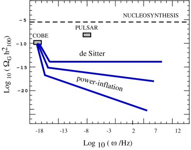
5.2 The graviton spectrum in minimal pre-big bang models
According to the pre-big bang scenario, the very early cosmological evolution starts from a state approaching the string perturbative vacuum, goes through an initial low-energy phase driven by the dilaton kinetic energy, and then necessarily reaches a purely “stringy” and quantum regime of high curvatures and large couplings. In that regime, the perturbative expansion of the string effective action becomes inappropriate (see Section 8), and the details of the background kinematics become (with present understanding) uncertain and strongly model-dependent; for the illustrative purposes of this subsection we shall assume that, in spite of these uncertainties, it is still possible to parametrize the kinematics of the string phase by a power-law evolution of the metric and of the dilaton field.
Neglecting the final matter-dominated era, which only affects the low-energy tail of the spectrum (and which is not very relevant to spectra that are growing very rapidly with frequency), we are thus led to consider a simple class of pre-big bang models in which the phase of accelerated evolution preceding the standard radiation era is divided into two physically distinct regimes: an initial, low-energy, dilaton-dominated phase, and a late, high-energy, string phase where and loop corrections become important (see Section 8). We shall denote by the time scale marking the transition to the high-curvature string phase and by the time scale marking the transition to the radiation-dominated cosmology (see Fig. 5.2), associated to a final curvature of order in string units. In the E-frame we may thus parametrize the following class of backgrounds:
| (5.10) |
The model seems to contain four parameters, or, equivalently, the curvature scales and coupling constants at the two transition epochs:
| (5.11) |
We may expect, however, that during the string phase the curvature scale stays controlled by the fundamental string mass ,
| (5.12) |
so that keeps constant in the S-frame, while it grows (driven by the dilaton) in the E-frame, where is a constant. This condition has two important consequences.
The first is that the final curvature scale, , turns out to be fixed by the present value of the fundamental ratio between the string and the Planck mass [404]:
| (5.13) |
The second is that, in the E-frame, according to the parametrization (5.10), we have , so that
| (5.14) |
i.e. .
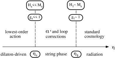
Since is fixed, and and are related, we are thus left with a “minimal” class of pre-big bang models [117, 306], characterized by a two-dimensional parameter space. As a convenient set of physical parameters we may choose, for instance, the duration of the string phase in conformal time, , and the value of the string coupling at the beginning of the high-curvature string phase.
For such a background, the effective potential of Eq. (4.56) is characterized by two transition scales, and the corresponding spectrum by two frequency bands, separated by the limiting frequency : we have in fact high-frequency modes with hitting the barrier (or crossing the horizon) during the string phase, and low-frequency modes with hitting the barrier during the dilaton phase. By applying the general procedure illustrated in the previous section one then finds the following spectral distribution [117]:
| (5.15) | |||||
(modulo logarithmic corrections, see Section 4.2). Such a spectrum has three important properties.
-
•
The low-frequency band is characterized by a nearly thermal (i.e., Rayleigh–Jeans) behaviour, , that simulates the low-energy part of a black-body spectrum.
-
•
At high frequencies the slope is at most cubic, but in general flatter, as , with .
-
•
The end-point values of the spectrum are approximately known, and fixed in terms of the fundamental ratio :
(5.16)
The spectral behaviour of this class of backgrounds, computed by perturbing the lowest-order string effective action, is expected to remain valid even when the corrections are included (to first order) in the perturbed action [278]: the spectrum remains the same, only the amplitude is slightly modified, with no appreciable consequence for an order-of-magnitude estimate (as confirmed also by recent numerical simulations, [149]). What remains model-dependent, however, is the position of the break in the spectrum, determined by the coordinates and . For comparison with the standard predictions of the de Sitter inflationary scenario, we have thus plotted in Fig. 5.3 three possible spectra, for a graviton background of pre-big bang origin, corresponding to different durations of the string phase, and to different slopes of the string branch of the spectrum.
It should be mentioned that the full spectrum of tensor metric perturbations has recently been computed for a regular class of minimal pre-big bang models, including in the linearized perturbation equations also the contributions from the higher-derivative and loop corrections needed for a smooth transition to the post-big bang regime [149]. It has been checked, in such a context, that the spectrum of the low-frequency modes , crossing the horizon in the low-curvature regime, is unaffected by the higher-order corrections. Also, it has been explicitly confirmed that the “string branch” of the spectrum () is flatter than at low frequency, and that its amplitude can be reliably estimated also by means of the low-energy perturbation equation. It has been found, however, that if the transition to the post-big bang regime goes through a phase described by the fixed-point solutions of the (first order in ) truncated string effective action (see Subsection 8.3), then the slope of the string branch of the spectrum is at least quadratic, i.e. still too steep for a possible detection by present gravitational antennas (see Subsection 5.4).
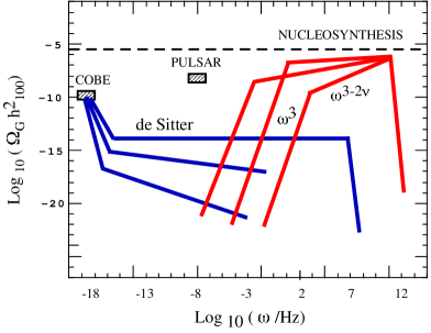
In any case, the graviton spectrum of the minimal pre-big bang scenario is monotonically growing and, as a consequence, the most constraining bound is provided by nucleosynthesis, as is evident from Fig. 5.3. The string branch of the spectrum can be extended (at least in principle) to arbitrarily low frequencies, provided that the slope is not too flat, to avoid a conflict with the pulsar bound. It should be stressed, however, that the nucleosynthesis bound applies to the total integrated energy density, and thus becomes more and more stringent as the spectrum is flatter and the string phase is longer.
Given our present ignorance of the dynamical details of the string phase, where high-curvature and quantum-loop effects are expected to play a significant role, the precise shape of the spectrum turns out to be (at present) strongly model-dependent (as also stressed by the examples analysed in [149]). It is remarkable that, in spite of this uncertainty, it may be possible to provide an accurate (and rather model-independent) estimate of the theoretically allowed region for the expected spectrum, in the plane of Fig. 5.3.
5.3 Allowed region in the – plane
The determination of the allowed region requires a precise estimate of the coordinates of the end-point of the spectrum [118], and . The first one is the maximal amplified frequency, corresponding approximately to the production of one graviton per polarization mode and per unit of phase-space volume. The present value of this frequency is:
| (5.17) |
The second one is the associated peak value,
| (5.18) |
(from Eq. (4.92)). The present value of contains two elements of intrinsic uncertainty.
A first uncertainty corresponds to the identification . It is true that the final transition scale should be controlled by the string mass scale, but the exact value of might be slightly different from . This uncertainty is expected to be small, however, and can be neglected in a first approximation.
A second (and just moreimportant) uncertainty is associated to the rescaling of from the transition time down to . There are in fact two possibilities. If the CMB radiation that we observe today was all produced by the transition at , together with the gravitons, then the ratio remains fixed throughout the subsequent cosmological evolution from down to , the redshift of is known and can be computed exactly. If, on the contrary, there was some process of radiation production due to some reheating phase occurring at time scales much later than , then the present value of the ratio can be arbitrarily diluted with respect to its original value at , corresponding to a redshift of which is in principle unknown and arbitrarily large.
To take this last possibility into account, we may introduce the phenomenological parameter , representing the fraction of the present CMB entropy density due to all reheating processes following the end of the string phase at . This parameter is defined by
| (5.19) |
where and are the thermal entropy density of the CMB background at and , defined in terms of the temperatures () and of the numbers () of particle species contributing (with their own statistical weight) to the entropy:
| (5.20) |
By using , and assuming thermal equilibrium at , we then obtain [118]:
| (5.21) |
where K is the present CMB temperature.
At fixed , the main uncertainty on the end-point values is thus controlled by the fundamental ratio , as illustrated in Fig. 5.4, where the boxes around the end point display an uncertainty corresponding to the allowed range . By varying , the end point moves along the thin line with slope . The present peak intensity is thus depressed for large values of ; however, as we can see from the picture, even if of the present entropy had been produced during the latest stage of evolution, the intensity of the relic graviton background would stay well above the full line labelled “de Sitter”, which represents the most optimistic prediction of the standard inflationary scenario in this frequency range.
We note, finally, that the same numerical value of the ratio also controls the amplitude of the bulk graviton spectrum possibly produced in the context of a pre-big bang scenario with large extra-dimensions [36, 32]. Indeed, even if the -dimensional Planck scale is smaller (for larger volumes of the internal space), the string scale is correspondingly lowered, so as to keep the grand-unified gauge coupling in the above allowed range.
The above discussion refers to the minimal models illustrated in the previous subsection, where the end point and the peak of the spectrum are strongly correlated, according to Eq. (5.21). Actually, what is really fixed in the pre-big bang scenario is the maximal height of the peak, but not necessarily the position in frequency, and it is not impossible, in more complicated, non-minimal models, to shift the peak to lower frequencies.
In the minimal models, in fact, the end of the string phase coincides with the freezing of the coupling parameter , and with the beginning of the standard radiation era. In non-minimal models [279] (see also [46]) the coupling is still very small at the end of the string phase, , the dilaton keeps growing in a decelerated way while the curvature starts decreasing, and the produced radiation becomes dominant only much later (such models are also important in the context of reheating, see [133]).
The main difference between the two classes of models is that in the non-minimal case the effective potential appearing in the canonical perturbation equation is non-monotonic, so that the highest frequency modes re-enter the horizon during the intermediate dilaton-driven phase that follows the string phase and preceds the beginning of the radiation era. This modifies the slope of the spectrum in the high-frequency sector, with the possible appearance of a negative power [279] (see also [263]). The gravity-wave spectrum may thus become non-monotonic, and the peak may no longer coincide with the end point, as illustrated in Fig. 5.4. A similar behaviour for the spectrum is also obtained in the context of non-minimal pre-big bang models that include a phase of “thermal inflation”, or a period of early matter domination [481]. A phase of matter-dominated pre-big bang evolution can also produce a flat graviton spectrum [252], but in that case the intensity of the relic background is much smaller than the peak values reported in Fig. 5.4.
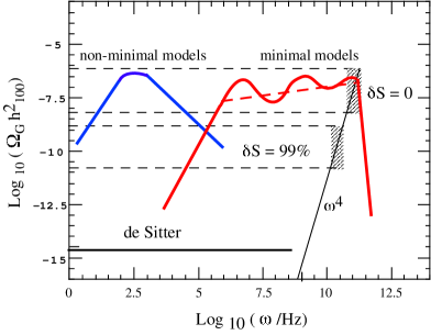
These are good news from an experimental point of view, because they suggest the possibility of a large detectable signal, even at frequencies much lower than the gigahertz band. However, they also provide a warning against too naive an interpretation and extrapolation of possible future experimental data, because of the complexity of the parameter space of the string cosmology models. It should be noted, for this purpose, that the spectrum associated to the string phase could be monotonic only on the average, and could locally oscillate even in minimal models [134], as illustrated by the wavy line appearing in the high-frequency branch of the spectrum of Fig. 5.4.
Given the present theoretical uncertainties, it seems appropriate to define the maximal allowed region for the expected graviton background, i.e. the region spanned by the spectrum in the plane when all its parameters are varied. Such a region is illustrated in Fig. 5.5, for the (phenomenologically interesting) high-frequency range Hz. The figure emphasizes the possible, large enhancement (of about eight orders of magnitude) of the expected graviton background in pre-big bang models, with respect to the standard inflationary scenario. The maximal allowed intensity of the graviton background coincides with the upper border of the strip with in Fig. 5.4, i.e. from Eq. (5.21):
| (5.22) |
Note that this upper limit is automatically compatible with the nucleosynthesis bound, Eq. (5.4), even if the spectrum is nearly flat from the end point down to the hertz scale.
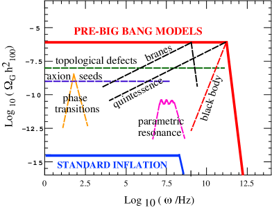
This maximal amplitude can be conveniently expressed in terms of a useful experimental parameter, the strain density , defined by [256]
| (5.23) |
and related to the energy density (5.7) (using the stochastic condition (4.67)) by [279, 464]:
| (5.24) |
The minimal experimental sensitivity required for a direct detection (by a single gravitational antenna) of the maximal background (5.22) of pre-big bang gravitons is thus given by [118]
| (5.25) |
This shows that the minimal sensitivity needed to reach the border of the allowed region grows with the frequency band to which the detector is tuned, even if such a border is the same at all frequency scales (see Eq. (5.22) and Fig. 5.5). This effect may favour –from an experimental point of view– detectors working at lower frequencies. Unfortunately –from a theoretical point of view– the probability of a large background intensity seems to be larger at higher frequencies, since the typical spectrum of pre-big bang models is growing. It is important to stress, however, that the minimal required sensitivity (5.25) may be somewhat relaxed, for realistic detection strategies in which the search for a stochastic background proceeds through the cross-correlation of the outputs of two independent detectors (see the next subsection).
The relic background associated with the parametric amplification of the vacuum fluctuations is compared, in Fig. 5.5, with other possible backgrounds of primordial origin, obtained with different mechanisms: graviton radiation from cosmic strings [138, 69] and other topological defects [474], from axion seeds [609], from bubble collision at the end of a first-order phase transition [591], and from parametric resonance of the inflaton oscillations [412, 67]. The spectrum obtained from a phase transition, plotted in the figure, refers to a typical reheating temperature – GeV, but higher peak values are possible for higher [591].
Also shown in the figure is the linearly growing spectrum obtained in recently proposed models of “quintessential” inflation [511, 335] and of “brane-world” inflation [551], and a thermal black-body spectrum corresponding to a present temperature K. In the standard inflationary scenario, a thermal background might originate at the Planck scale, when the temperature is high enough to maintain gravitons in thermal equilibrium. Such a background, however, should be strongly diluted (with respect to the present CMB radiation) by the action of the subsequent inflationary phase, occurring at curvature scales lower than Planckian. As a consequence, the surviving spectrum should correspond today to an effective temperature so depressed as to be practically invisible. In the context of the pre-big bang models, on the contrary, a thermal spectrum like that of Fig. 5.5 could be simulated by the sudden transition of the low-energy dilaton-driven phase to the standard radiation-dominated era – corresponding, for instance, to a minimal model of Section 5.2 with .
It may be noted that all the primordial backgrounds of Fig. 5.5 are higher (in intensity) than the background obtained from the amplification of the vacuum fluctuations in the standard inflationary scenario, but not higher than the analogous background expected in the context of the pre-big bang scenario. In any case, given the rich phenomenology of possible spectra, it seems appropriate to report at this point the experimental sensitivities of present gravitational antennas, referred in particular to the frequency range of Fig. 5.5. This will be the subject of the next subsection.
5.4 Experimental sensitivities
The limiting sensitivity (5.25) (corresponding to the upper border of the allowed region in Fig. 5.5) is unfortunately too high for the detectors that are at present in operation: the cryogenic, resonant-mass, gravitational antennas (see [521] for a review). In fact, if we take for instance the resonant bar NAUTILUS [174], the resonance frequencies are at and Hz and, at these frequencies, the strain sensitivity is approximately
| (5.26) |
With some improvements, the sensitivity is expected to reach in a few years the target value . Similar resonance frequencies (around Hz) and similar sensitivities are also typical of the other resonant detectors such as ALLEGRO [362], AURIGA [529], and EXPLORER [507]. The resonant bar NIOBE [375], however, is working at a smaller frequency ( Hz) and could reach, in principle, a slightly better sensitivity.
Interferometric detectors, such as LIGO [5], VIRGO [146], GEO600 [449] and TAMA300 [406], are already basically built and will soon become operative. The best planned sensitivity, for the first-generation instruments, is around
| (5.27) |
very similar to the present bar sensitivities. This sensitivity, however, is available at a smaller frequency band, Hz, and thus corresponds to a smaller limit in terms of the energy density of the graviton background (see Eq. (5.24)). In practice, the interferometers of first generation will be directly sensitive to – , better than resonant bars, which can at most reach the critical density, but still well above the border of the allowed region.
In order to approach the border sensitivity , we must wait for the second (and higher) generation of interferometers. The Advanced LIGO project [445], for instance, might lead to a two orders of magnitude improvement of the sensitivity (5.27), at Hz, thus reaching the borderline (5.22). An even better result is expected for the space interferometer LISA [380], whose goal is to reach the strain sensitivity [363] Hz-1/2 in the frequency band from to mHz, corresponding (in this band) to the remarkable limit .
Another interesting possibility concerns resonant detectors with spherical (or truncated icosahedron) geometry, such as the TIGA [388, 482] or SFERA [40] projects. Hollow spheres [173] are particularly promising: a large copper–aluminium detector ( – m in diameter), pushed to its extreme quantum limit may reach a strain sensitivity222M. Cerdonio and L. Conti, private communication. Hz-1/2, with resonant frequencies of and Hz (the resonance frequency can be tuned, in principle, by varying the geometrical radius of the sphere). Such a limiting sensitivity can be approached by the recently proposed wide-band “dual-sphere” detector [157], which consists of a massive solid sphere suspended inside a larger hollow one. In that case, a sapphire detector of an overall size of m could reach a strain sensitivity , for frequencies between and kHz.
Concerning higher frequencies (well above the kilohertz), the only possibility at present seems to be the use of resonant electromagnetic cavities [513, 535] or waveguides [188]. There are also recent experimental studies for detecting small displacements based on two coupled microwave cavities [81]: such a detector reaches the maximum sensitivity when the frequency of the incident gravitational wave is equal to the frequency-difference of the two cavity-modes. In this way, it seems possible at present to reach the strain sensitivity Hz-1/2 for frequencies around the kilohertz range [161]. Unfortunately, however, this value is well above the minimal required sensitivity (5.25).
As shown explicitly by the above examples, the limiting sensitivity (5.25) seems not to be within easy reach of present technology, for the case of a single detector. In addition, an unambiguous detection of a stochastic gravity-wave background with a single experimental apparatus would require a complete and exact knowledge of all the intrinsic instrumental noises, and of all the backgrounds of different origins that could interact with the gravitational antenna. Fortunately, an efficient answer to both difficulties is known: it is provided by the cross-correlation of the outputs of two (or more) detectors [163, 256, 14, 18].
Suppose that the outputs of two detectors, , , are correlated over an integration time , to define a signal:
| (5.28) |
Here is a real “filter” function, determined so as to optimize the signal-to-noise ratio (SNR), defined by an ensemble average as:
| (5.29) |
The outputs contain the physical strain induced by the cosmic background, , and the intrinsic instrumental noise, . The two noises are supposed to be uncorrelated (i.e. statistically independent), , and much larger in magnitude than the physical strains, . Also, the cosmic background is assumed to be isotropic, stationary and Gaussian, with . It follows that [18]:
| (5.30) |
The physical strain is given by the projection of the metric fluctuation (computed at the detector position ) over the detector response tensor , which characterizes the spatial orientation of the arms of the -th detector. If is a unit vector specifying a direction on the two-sphere, and is the gravity-wave polarization along , we can expands the strain in momentum space as
| (5.31) |
where denotes the angular integral over the unit two-sphere, and the index labels the two polarization modes of the wave; is the so-called “pattern function”, depending on the geometry of the detector. Note that in the above equation we have used the proper momentum , even if the cosmological variation induced by the expansion of the scale factor is negligible over a typical experimental time scale . Note also that, for a better comparison with experimental variables, we have used units in which , so that, for a gravity wave, (but not in general for massive waves, see Section 6.4).
For an isotropic, unpolarized and stationary background we can then use the stochastic condition to define [18, 464]
| (5.32) |
(the integration over the angular variables then reproduces Eq. (5.23)). By inserting the momentum expansion into Eq. (5.30), and assuming, as usual, that the observation time is much larger than the typical time intervals – for which , we finally obtain, using Eqs. (5.23) and (5.24):
| (5.33) |
where is the filter function in momentum space, and is the so-called “overlap-reduction function”:
| (5.34) |
Here is an overall normalization factor, depending on the type of the detectors (for two interferometers, a convenient choice is , see [18]; see [464] for the normalization of different antennas).
We now need to compute the variance , which, for uncorrelated noises much larger than the physical strains, can be expressed as [18]:
| (5.35) |
Introducing the (one-sided) noise power spectrum in momentum space, , defined by
| (5.36) |
and assuming as before that is much larger than the typical correlation intervals – , – , we obtain
| (5.37) |
The optimal filtering is now determined by the choice (see [18] for details)
| (5.38) |
where is an arbitrary normalization constant. With such a choice one finally arrives, from Eq. (5.33) and (5.38), to the optimized signal-to-noise ratio:
| (5.39) |
The background can then be detected, with a detection rate , and a false-alarm rate , if [18]:
| (5.40) |
Armed with the above results, it is now possible to estimate the minimum detectable background at a given confidence level, for any pair of gravitational antennas of given noise power spectrum and overlap . The correlation of all existing pairs of interferometers has been studied in [45] and [18]. With the sensitivities of the first-generation interferometers, for an observation time months, a detection rate of , a false-alarme rate of , and a flat graviton spectrum const, the minimum detectable value is
| (5.41) |
This value can be improved only slightly by increasing the number of correlated detectors. With the planned sensitivity of Advanced LIGO, however, one obtains the much better limit [14, 18]:
| (5.42) |
The correlation between two resonant bars, and between a bar and an interferometer, has been studied in [41, 42, 615, 45]. The minimum detectable values for the VIRGO-AURIGA or VIRGO-NAUTILUS or AURIGA-NAUTILUS pairs is at present [464] a few (depending on the bar orientation) for a flat spectrum, one year of observation, at the confidence level. The correlation of two spherical detectors seems to be more promising, however. Two spheres (of m diameter) located at the same site could reach a sensitivity [615] . Also, studies reported in [173] suggest that the correlation of hollow spheres could reach .
All the above results refer to a flat graviton spectrum. The signal-to-noise ratio, and therefore the sensitivity, depend, however, on , and then on the slope of the spectrum (see Eq. (5.39)), as also stressed in [464, 47]. The sensitivity to a growing spectral distribution such as that predicted by pre-big bang models has been computed in particular in [15, 594] and [46, 48], for a pair of LIGO and a (virtual) pair of VIRGO interferometers, respectively. The minimum detectable intensity of the background, in that case, does not show any improvement with respect to a flat spectrum; on the contrary, the sensitivity could even suffer from a slight decrease, if the maximum of the signal is near the border of the accessible frequency band, where the noise of the interferometer is higher.
Finally, the cross-correlation in the case of space interferometers such as LISA has recently been discussed in detail [595] by taking into account that, at lower frequencies, the sensitivity to a stochastic graviton background of primordial inflationary origin is fundamentally limited by the possible presence of other astrophysical backgrounds, generated at much later times, due for instance to binary systems of compact objects that cannot be resolved as individual sources. A detailed analysis, performed for the cross-correlation of two identical LISAs, leads to a minimum detectable signal , in the mHz range, for a flat spectrum. The three arms of LISA could also be combined in such a way as to simulate two inteferometers located in the same place; unfortunately, they would be rotated by an angle of with respect to one another, and the corrresponding overlap function would be identically zero over the whole frequency range. This is the reason why two space interferometers are needed, even in that case.
To conclude this subsection, let us recall the best (direct) experimental upper bound existing at present on the energy density of a stochastic graviton background, which has been obtained from the cross-correlation of the two resonant bars NAUTILUS and EXPLORER [38, 39]:
| (5.43) |
This results corresponds to a very small observation time ( hours), and it is thus far from the theoretical upper limit (5.25), but the future perspectives seem to be promising, as reported in the above discussion. The cross-correlations of advanced (ground-based) interferometers, space interforemeters, spheres, hollow spheres, are all expected to cross the borderline sensitivity (5.25), and then to explore, in a very near future, the allowed region of the string cosmology spectrum. Thus, future data from gravitational antennas will directly constrain the parameter space of the minimal and non-minimal classes of pre-big bang models considered in this section.
We should add, finally, that useful information and constraints on the relic graviton background will also be obtained from future measurements of the CMB polarization [560, 401, 433]. The presence of a gravitational-wave background should in fact induce a characteristic “curl component” in the large scale CMB polarization [402], which might be detectable by dedicated experiments (already at the sensitivity level of the Planck satellite [522]) for the gravitational spectra predicted by the standard inflationary models. No polarization signal is expected to be detectable, on the contrary, for the graviton spectra of pre-big bang models, whose amplitude is extremely suppressed at the large scales accessible to the polarization experiments (see, however, Ref. [252] for possible exceptions).
6 Relic dilatons
The effective action of string cosmology always contains at least two fundamental fields, the metric and the dilaton. The amplification of the dilaton fluctuations leads to dilaton production, just like the amplification of the transverse, traceless components of the metric fluctuations leads to graviton production. The possible formation of a stochastic background of relic dilatons [272, 322, 277], with statistical and squeezing properties similar to those of the graviton background, is one of the most peculiar phenomenological aspects of pre-big bang models.
The main physical difference with the graviton background, discussed in the previous section, concerns the possible contribution of the mass to the dilaton spectrum (see Subsection 6.1). The dilaton should indeed be massive, according to conventional models of supersymmetry breaking [53]. Also, the dilaton must be massive if it is coupled non-universally to macroscopic matter with gravitational strength [578, 238], in order to avoid unacceptable violations of the equivalence principle. The value of the dilaton mass, however, is largely unknown from a theoretical point of view. There are phenomenological constraints on the mass, but they depend on the effective coupling of dilatons to macroscopic matter, which we shall discuss in Subsection 6.2. The value of the coupling, in turn, is strongly model-dependent [198, 199], and phenomenologically constrained, at present, only by tests of the equivalence principle and of Newtonian gravity available on a macroscopic scale [254, 381].
As a consequence, the present amplitude of the relic dilaton background, controlled by the string and dilaton mass, is more uncertain than in the graviton case. This is disappointing, on the one hand, as it prevents the existence of an unambiguous link between the spectral properties of the dilaton background and the parameters of pre-big bang models. On the other hand, however, it leaves open two interesting phenomenological possibilities: a relic background of non-relativistic dilatons could represent a significant fraction of the present dark matter density [272] (see Subsection 6.3) and, if the mass is small enough, it could be detectable by the cross-correlation of gravitational antennas [288] already at the sensitivity level of enhanced interferometric detectors [318], as will be discussed in Subsection 6.4.
6.1 Dilaton production
In this subsection we will estimate the spectral distribution of the dilatons obtained from the amplification of the vacuum fluctuations, in the context of pre-big bang models. There are, of course, also other cosmological mechanisms of production, such as particle collisions at high (Planckian) temperature, coherent oscillations around the minimum of the scalar potential (and more exotic mechanisms, such as dilaton radiation from cosmic strings; see for instance [201]). We will concentrate here on the parametric amplification because, even if the temperature remains too low to allow thermal production, and oscillations are avoided through a symmetry that ensures the coincidence of the minima of the potential at early and late times [200], quantum fluctuations cannot be eliminated; also, they may be expected to represent the dominant source [458] when the inflation scale is not smaller than about GeV, as in the context of the pre-big bang scenario.
The production of dilatons through the amplification of the quantum fluctuations of the scalar background is very similar to the amplification of tensor perturbations, discussed in Section 5. Unlike the graviton case, however, the analysis of dilaton perturbations is complicated by their coupling to the scalar component of metric perturbations, and to the scalar perturbations of the matter sources. The matter sources may even be absent from the pre-big bang phase, but they are certainly not absent when dilatons re-enter the horizon, in the radiation- and matter-dominated epoch.
In order to discuss this effect, we shall work in the E-frame, in the longitudinal gauge, and we shall assume that the -dimensional, homogeneous and isotropic, unperturbed background is driven by the dilaton and by a perfect-fluid model of matter sources. Our independent variables are the scalar metric, dilaton and fluid perturbation, respectively , , , , , , defined by:
| (6.1) |
In the E-frame the fluid sources are non-trivially coupled to the dilaton, and the unperturbed equations take the form (in units ):
| (6.2) |
where the numerical factor arises from the conformal transformation of the S-frame string cosmology equations (see for instance Eq. (2.113)). The perturbation of these equations, for the components, gives , while the combination of the perturbed and dilaton equation leads to the vector-like equation for the doublet , representing the Fourier components of the metric and of the dilaton fluctuations [322]:
| (6.3) |
Here are , time-dependent mixing matrices, whose explicit form depends on the unperturbed solutions, on the equation of state , on the model of fluid perturbations and, finally, on the possible presence of a dilaton potential . In particular, for an unperturbed background in which the dilaton can be parametrized by , with const, the mixing matrices are given by
| (6.4) | |||
| (6.5) | |||
| (6.6) |
where the primes denote differentiation with respect to conformal time, except for the potential, where . Once is known, the density and velocity contrast are fixed in terms of and by two additional equations , , following, respectively, from the perturbation of the and background equations:
| (6.7) | |||
| (6.8) |
An exact computation of the dilaton fluctuations thus requires an exact solution of the coupled equations (6.3). Also, the correct normalization of the dilaton spectrum to the quantum fluctuations of the vacuum requires in general the diagonalization of the system metric + dilaton + fluid sources, to find the normal modes of oscillation satisfying canonical commutation relations, as discussed in Subsection 4.3.
This program can be easily performed if we limit ourselves to a dilaton-dominated pre-big bang phase with negligible matter sources (), and we consider the high-frequency part of the spectrum, i.e. those modes re-entering the horizon during the radiation-dominated phase, characterized by adiabatic fluid perturbations () and by the dilaton frozen () at the minimum of the non-perturbative potential (). In that case the canonical variables are known, and one finds that the perturbation equations are decoupled in the radiation era, where the canonical variable for the dilaton fluctuation is simply (in ) , and satifies the (covariant) Klein–Gordon equation (from the system (6.3)):
| (6.9) |
For relativistic modes, of proper momentum , the solution describes (in conformal time) free plane-wave oscillations, and we thus recover for the dilaton the same spectrum as in the graviton case [322]. Working in the framewok of minimal pre-big bang models (see Subsection 5.2) we find, in particular, that the dilaton modes amplified during the low-energy phase are characterized by the distribution . In order to include the possible corrections due to the modified kinematics of the high-curvature string phase, we may thus parametrize the high-frequency, relativistic branch of the dilaton spectrum as
| (6.10) |
Here is the slope parameter corresponding to a growing, but unknown, spectral index; and are the parameters associated to the transition scale of minimal pre-big bang models. It should be noted that, unlike the graviton case, we no longer identify proper momentum and proper frequency , as we are dealing, in principle, with massive particles for which .
The above spectral distribution cannot be extrapolated down to momentum scales re-entering the horizon after equilibrium, since in the matter era the perturbation equations (6.3) are no longer decoupled, even if the dilaton background is frozen at the minimum of the potential (they remain coupled not only in the longitudinal gauge, but also in the uniform-curvature gauge, defined in Eq. (4.41)). In addition, for modes of low enough momentum , we must take into account the non-relativistic correction to the above spectrum (indeed, even if the mass term is negligible at the inflation-radiation transition scale, i.e. , the proper momentum is redshifted with respect to the mass in the subsequent radiation era, and all modes tend to become non-relativistic).
When including the mass term, the general solution of Eq. (6.9) in the radiation era can be written in terms of the parabolic cylinder functions [6], and its matching to the (massless) pre-big bang solution provides the correct inclusion of the mass contributions to the spectrum. The details of the computation are the same as in the case of massive axions [225], and will be reported in Section 7. Here we simply note that if a mode becomes non-relativistic well inside the horizon, i.e. when , then the number of produced dilatons is fixed after re-entry, when the mode is still relativistic, and the effect of the mass is a simple rescaling of the energy density: . If, on the contrary, a mode becomes non-relativistic outside the horizon, when , then the final energy distribution turns out to be determined by the background kinematics at the exit time, and the effective number of non-relativistic dilatons has to be adjusted by continuity, in such a way that has the same spectral distribution as in the absence of mass. The two regimes are separated by the limiting momentum scale of a mode that becomes non-relativistic just at the time it re-enters the horizon [272, 322]:
| (6.11) |
Taking into account such mass corrections, we may thus add to the relativistic dilaton spectrum (6.10) two lower-frequency, non-relativistic bands (see also [293]):
| (6.12) |
| (6.13) |
Note that these spectral distributions evolve in time like , and thus keep constant during the matter-dominated era, for . Note also that, for simplicity, the non-relativistic corrections have been referred to a single relativistic branch, with for the low-energy pre-big bang phase, and with for the string phase. However, the mass corrections can be extended without difficulty to a more general situation in which there are two (or more) branches in the relativistic spectrum, as in minimal pre-big bang models characterized by the two frequency bands and (separated by the string scale ). In such a case, the non-relativistic corrections will affect only the lower, or also the higher, frequency band of the spectrum, depending on whether or , respectively.
If the dilaton mass is large enough, the present amplitude of a possible relic dilaton background is thus controlled by the (unknown) value of its mass. The cosmological bounds on the spectrum can thus be translated into phenomelogical bounds on the mass, depending (but only weakly) on the spectral index . Such bounds are to be combined with other, model-dependent bounds on the mass related to the strength of the effective dilaton coupling to macroscopic matter, which will be discussed in the next subsection.
6.2 Effective coupling to macroscopic matter
The motion of macroscopic test bodies in an external, non-trivial, gravidilaton background is in general non-geodesic, if the body posseses a non-negligible dilatonic charge. Suppose in fact that the interaction of macroscopic matter with the external scalar-tensor background is described by the effective action of Subsection 4.1:
| (6.14) |
(in units ), where the Brans–Dicke parameter is equal to for the lowest-order action of string theory, and we have added the action for the matter fields describing a test body non-trivially coupled to the metric and to the dilaton. The variation with respect to and provides respectively the field equations (with ):
| (6.15) |
containing two source terms: the “gravitational charge density” (the dynamical stress tensor), and the dilatonic charge density :
| (6.16) |
The combination of the above equations, and the use of the contracted Bianchi identity , then implies the covariant conservation of the stress tensor, , for any , provided . If the dilatonic charge is non-zero, however, the gravitational charge density is not separately conserved; for , in particular, we obtain from Eqs. (6.15):
| (6.17) |
To obtain the equation of motion of the test body we now integrate this equation over a space-like hypersurface, and perform a multipole expansion of the external metric and dilaton field around the world line of the centre of mass of the body [508]. In the point-particle approximation, the gravitational and dilatonic charge densities are defined by
| (6.18) |
(where ), and we obtain the general equation of motion [286]
| (6.19) |
where is the dilatonic charge per unit of gravitational mass (representing the relative strength of scalar to tensor forces).
It is now evident that a non-zero induces deviations from pure geodesic motion, and that the experimental tests on the gravitational forces provide limits on the allowed values of the dilaton charge. Large values of can only be allowed if the dilatonic interactions, on a macroscopical scale, are suppressed by a sufficiently small range. We may also note, for future reference, that the relative acceleration between two world lines satisfying Eq. (6.19), with infinitesimal separation , is given by a generalized equation of “geodesic deviation” [286]:
| (6.20) |
We shall come back to this point in Subsection 6.4.
A precise estimate of , in a string theory context, should start from the effective action describing the coupling of the dilaton to the fundamental quark and lepton fields building up ordinary macroscopic matter. Including all possible loop corrections, such an action can be written in the general form
| (6.21) |
where are the dilatonic “form factors”, to all orders in the loop expansion, and where we have used, for simplicity, a scalar model of fundamental matter fields . The effective masses () and dilaton couplings () of the fields can then be defined in terms of the canonical rescaled variables , which diagonalize the kinetic term and have canonical dimensions. In the low-energy limit we may expand the interaction Lagrangian around the value of the dilaton, which extremizes the effective potential [578, 322]:
| (6.22) |
Performing the computation in both the String and Einstein frames [286], we find that the dilatonic charges per unit of gravitational mass, respectively and in the two frames, are related by (in units ):
| (6.23) |
Unless is fine-tuned to 1 (corresponding to an exact Brans–Dicke theory for the field ), the dilatonic charge is non-vanishing in both frames and, in general, is non-universal, as the form factors are different for different fields.
As originally stressed in [578], this suggests a large dilatonic charge ( – ) for the confinement-generated components of hadronic masses, and a smaller charge, but of gravitational intensity (), for leptonic masses (see also [238, 31]). If this is the case, the total charge of a macroscopic body is large (in gravitational units), and composition-dependent.
Consider in fact a macroscopic body of mass , composed of baryons with mass and charge , and electrons with mass and charge . The total dilatonic charge per unit mass, , for , , is then
| (6.24) |
where is the mass of the body in units of baryonic masses. Since , the total dilaton charge of a macroscopic body is controlled by the dilaton coupling to baryons, , it is of the same order of magnitude in the String and Einstein frames, , and it is composition-dependent (as depends on the internal nuclear structure), with variations, across different types of ordinary matter, which are typically of order [286]
| (6.25) |
The only way to escape the conclusion that the dilaton charge of macroscopic bodies is composition-dependent and large is to assume that the coupling of the dilaton to the fundamental matter fields is universal (the same for all fields, to all orders in the loop expansion), and to choose appropriate values of the parameters in the resulting scalar-tensor effective action. This is not impossible, as illustrated by the model discussed in [198, 199]. In such a context, if the effective coupling is appropriately suppressed (), the dilaton mass can be very small, or even vanishing. The precise measurements of the gravitational force over quite a wide range of distances provide in fact exclusion plots in the plane (), which constrain the dilaton charge as a function of its mass (see for instance [254] for a comprehensive compilation of experimental bounds on possible “Yukawa” deviations from Newtonian gravity, both for universal and composition-dependent interactions).
For later use, let us recall here the phenomenological bound on the dilaton mass for a large, composition-dependent dilaton charge [254]:
| (6.26) |
In the opposite, small-coupling regime, and in the mass range appropriate to gravitational antennas, i.e. from to eV, corresponding to the frequency range from to Hz, the phenomenological bounds [254] can be parametrized as
| (6.27) |
for universal dilaton interactions, and
| (6.28) |
for composition-dependent interactions.
We can now discuss the intensity of the relic-dilaton background, taking into account two distinct phenomenological possibilities: 1) (heavy) massive dilatons, gravitationally (or more strongly) coupled to macroscopic matter, and 2) massless (or very light) dilatons, universally (and weakly enough) coupled to matter. In the last case, the conclusions about a possible detection of the dilaton background produced by pre-big bang models are not completely negative, as we shall illustrate in Subsection 6.4.
6.3 Bounds and allowed windows for heavy (strongly coupled) dilatons
Let us first discuss the large-coupling case (the most unfavourable, probably, for a direct detection). In such a case eV, so that today even the highest mode present in the spectrum, , is non-relativistic (see Eq. (5.16)):
| (6.29) |
(since ). In other words, the branch (6.12) of the dilaton spectrum extends from to . We shall start assuming that the slope is steep enough, , for the high-frequency branch from to to represent the dominant part of the spectrum. In that case all the cosmological bounds that apply to the total integrated dilaton energy density will become -independent [272, 322] (the case will be considered below).
When the spectrum becomes non-relativistic, the dilaton energy density starts to grow with respect to the radiation energy density, . In particular, when the Universe enters the matter-dominated era, the non-relativistic part of the dilaton spectrum remains frozen (in critical units) at the value reached at the time of the matter-radiation equilibrium, . The present value of the dominant (non-relativistic) branch of the spectrum can thus be expressed in terms of the equilibrium scale as:
| (6.30) |
where we have used Eq. (6.12), and the fact that = , assuming radiation-dominance from to . We recall that, for the equilibrium curvature scale, .
A first important constraint [239, 241, 206] is now obtained by imposing that the energy density stored in the coherent oscillations of non-relativistic dilatons, integrated over all modes, remains smaller than critical, at all times:
| (6.31) |
For this gives the stringent constraint
| (6.32) |
which represents, in this context, the most restrictive upper bound on the mass of (not yet decayed) dilatons. For keV MeV a more restrictive constraint on is provided in principle by the observations of the astrophysical background of diffuse -rays [201]; such a range of masses, however, tends to be excluded, as will be shown below, in the context of pre-big bang models where the inflation scale is controlled by the string mass, .
The critical density bound (6.32) can be evaded if the dilatons are heavy enough to decay, so that the energy stored in their coherent oscillations was dissipated into radiation before the present epoch. The decay scale is fixed by the decay rate (for instance into two photons) as
| (6.33) |
(which implies, in particular, that the produced dilatons have not yet decayed, today, only if MeV). The decay, however, generates radiation, reheats the Universe, and is associated in general to a possible entropy increase
| (6.34) |
where and are the final reheating temperature and the radiation temperature immediately before dilaton decay, respectively. The decay process is thus the source of additional phenomenological constraints on the dilaton spectrum, which are complementary to the critical bound (6.32), as they imply in general a lower bound on the dilaton mass.
In order to discuss the consequences of dilaton decay let us note, first of all, that the induced reheating is significant (, ) provided dilatons decay when they are dominant with respect to radiation, i.e. for , where is the curvature scale marking the beginning of dilaton dominance. Such a scale is defined by the condition , where is obtained by integrating over all modes the dominant branch (6.12) of the non-relativistic dilaton spectrum. For this leads to
| (6.35) |
from which
| (6.36) |
(we have assumed that such a scale belongs to the radiation era, ; otherwise, the bound we obtain is less stringent).
At the given scale , the radiation temperature is fixed by the Einstein equations (and by the Sefan law ) as
| (6.37) |
where is a dimensionless numerical factor of order unity, which disappears from the final estimate. The radiation temperature at the epoch of dilaton decay, , is then obtained by the adiabatic rescaling
| (6.38) |
since the scale factor evolves like during the phase dominated by the non-relativistic dilatons. After the decay, on the other hand, the Universe becomes radiation-dominated, with a reheating temperature fixed by the decay scale as
| (6.39) |
and with a final, total entropy increase [272, 322]:
| (6.40) |
This entropy injection can in principle disturb nucleosynthesis and/or baryogenesis [239, 241, 206], and we should consider two possibilities.
If the reheating temperature is too low to allow nucleosynthesis, MeV, i.e. TeV, we must assume that nucleosynthesis occurred before, and we must impose
| (6.41) |
to avoid destroying the light nuclei already formed (more precise bounds can also be determined through a detailed analysis of photodissociation [240] and hadroproduction [218]).
If the reheating temperature is large enough to allow nucleosynthesis, MeV, i.e. TeV, the only possible constraint comes from primordial baryogenesis. The bound is model-dependent, but the constraint
| (6.42) |
seems to be sufficient [239, 241, 206] not to wash out any pre-existing baryon–antibaryon asymmetry (this bound could be evaded in the case of low-energy baryogenesis occurring at a scale ).
The above constraints can be easily extended to the case , see [272, 322]. Consider, for instance, the critical density bound. For the non-relativistic spectrum (6.30) has a peak at , which dominates the integral (6.31), and which leads to a total integrated energy density:
| (6.43) |
The bound now imposes [272, 322]
| (6.44) |
which for exactly reduces to the condition (6.32).
For the dilaton decay the situation is similar: if the total energy density is dominated by the contribution of , and all bounds become -dependent. The scale of dilaton dominance, obtained by equating to in the radiation era, becomes , and the corresponding increase of entropy is
| (6.45) |
Taking into account all bounds, we obtain the allowed region in the plane illustrated in Fig. 6.1. The allowed values are below the upper (bold) solid lines for a growing () spectrum [272], and below the lower (thin) solid lines for a flat () spectrum [343, 239, 241]. For the allowed region interpolates between the two limiting cases illustrated in the figure.
To the left, the region is bounded by the tests of the equivalence principle, Eq. (6.26), as we are considering dilatons with large couplings to macroscopic matter, . To the right, the mass is bounded by the condition (not shown in the picture), which has to be imposed to avoid overcritical density in case , when the produced dilatons are already non-relativistic from the beginning [322] (in that case there are no additional bounds, as dilatons decay before becoming dominant). Finally, the upper limit on the inflation scale, , is required to avoid overcritical production of massless particles since, for a growing spectrum, (see for instance Eq. (6.10)).
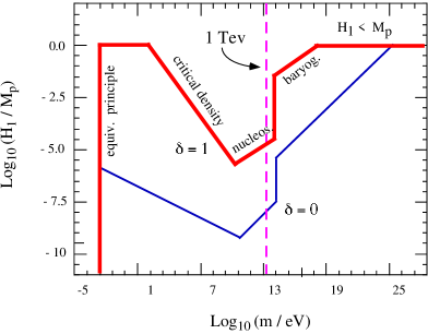
In the standard inflationary scenario the spectrum tends to be flat, and the “natural” value for the dilaton mass required by models of supersymmetry breaking [53], TeV, is not consistent with the preferred value of the inflation scale, , typically determined by the grand-unification phase transition (this is the so-called problem of the dilaton mass). In string cosmology the spectrum tends to be growing, the allowed region “inflates” in parameter space, and the TeV mass scale becomes marginally compatible with the wanted inflation scale. Unfortunately, however, in a string cosmology context, is expected to be determined by the string scale, and thus fixed around – , so that the problem remains.
A possible solution of this problem can be obtained in the presence of a late, post-inflationary reheating phase, preceding nucleosynthesis and dilaton decay, and producing a suitable dilution of the original dilaton density by the factor [277]
| (6.46) |
Here are, respectively, the thermal entropy density of the CMB radiation and the number of particles species in thermal equilibrium, at the beginning () and at the end () of this reheating process. An efficient reheating, , , reduces in a significant way the dilaton fraction of critical density : as a consequence, the scale (6.36) of dilaton dominance is lowered, the decay temperature (6.38) is raised, and the bounds on following from the entropy constraint () and the critical bound () are relaxed. Such a reheating is possible, for instance, in the context of models of “intermediate scale” inflation [532], or “thermal” inflation [459].
Even without such a relaxation, the minimal pre-big bang scenario leaves open two interesting mass windows, obtained by intersecting the allowed region of Fig. 6.1, for , with the allowed value of the string mass scale [404],
| (6.47) |
(under the assumption ). It follows that there are two possible ranges for the dilaton mass [277]:
| (6.48) |
illustrated in Fig. 6.2. The vertical solid line at the MeV mass scale, shown in Fig. 6.2, corresponds to a dilaton decay rate of the same order as the present Hubble scale, . To the right of this line all produced dilatons have already decayed, while to the left, and in particular inside the window of Eq. (6.48), dilatons are still around us, and could in principle be observed.
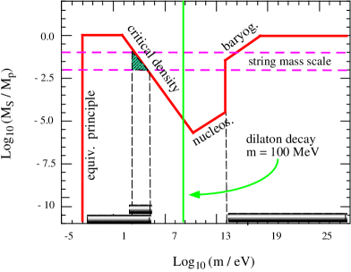
If, in addition, the mass is within the restricted range
| (6.49) |
obtained by intersecting the string mass scale with the critical density bound (6.32), then the produced dilatons could even saturate the critical density value, or at least could provide a significant fraction of the present cold dark-matter density [272], with
| (6.50) |
according to Eq. (6.30). It is important to recall, in such a context, that the possibility of a small dilaton mass is not theoretically excluded (in spite of the “standard” TeV mass range), as shown for instance by models of supersymmetry breaking with light dilatons [251]. Also, it is important to stress that the range of masses saturating the critical density bound moves to lower and lower values as the spectrum becomes flatter and flatter (see Eq. (6.44) with ). For , in particular, the critical bound is saturated by
| (6.51) |
corresponding to masses as small as eV (or lower).
Such values of mass are excluded neither theoretically nor experimentally, as discussed in Subsection 6.2, provided the dilaton coupling to macroscopic matter is sufficiently small, . It is then possible to imagine a cosmological scenario in which a relic background of non-relativistic dilatons, produced as a consequence of the pre-big bang evolution, could provide today a significant contribution to the critical energy density and, simultaneously, have a mass in the appropriate range to stimulate a resonant response of present gravitational antennas [288] (i.e. – eV). In that case, the high intensity of the background (not constrained by nucleosynthesis, as in the graviton case), could possibly compensate the weakness of the dilatonic charge of the antennas, and could determine in principle a detectable signal. This interesting possibility will be discussed in the next subsection.
6.4 Detection of ultra-light dilatons
A stochastic background of relic dilatons, produced by a phase of pre-big bang evolution, and light enough to have a lifetime larger than the present Hubble scale, could interact today in two ways with the existing gravity wave detectors: either indirectly, through a geodesic coupling of the detector to the scalar part of the induced metric fluctuations contained in the Riemann tensor [84, 83, 112, 565, 465, 494], or even directly through the non-geodesic coupling of the dilaton to the scalar charge of the detector [286, 288] (see Eqs. (6.19), (6.20)).
In the first case the coupling has a gravitational strength, but the amplitude of scalar metric perturbations, at the typical resonant scales of present detectors, could be much lower than the amplitude of the original dilaton fluctuations. In the second case the detector could be coupled to a background of very high intensity (of order in critical units), but with a coupling constant strongly suppressed for phenomenological reasons, as discussed in Subsection 6.2.
In order to take into account both possibilities, we will estimate the scalar-to-noise ratio associated to a stochastic dilaton background by assuming that the physical strains (), induced on a pair of gravitational antennas, vary in time like the scalar fluctuations that perturb the detectors, and are proportional to the scalar pattern functions through the scalar charges of the detectors [288, 318]:
| (6.52) |
Here is the polarization tensor of the scalar wave propagating along the direction, and is the detector response tensor (see Subsection 5.4); finally, for the coupling to scalar metric fluctuations, while for the direct coupling of long-range scalar fields.
We expand the strain in momentum space, taking into account the mass of the scalar fluctuations (),
| (6.53) |
and we use the stochastic condition which, for a scalar spectrum ,
| (6.54) |
can be written as
| (6.55) |
By imposing optimal filtering [18], and following the same steps as in Subsection 5.4 for the graviton case, we finally arrive at the signal-to-noise ratio [318]:
| (6.56) |
where is the total integration time, are the one-sided noise spectral density of the detectors, defined as Fourier transforms of the frequency , and is the overlap reduction function, defined in momentum space by:
| (6.57) |
(normalized so that for coincident and coaligned interferometers). For and we recover the signal-to-noise ratio (5.39), modulo a different normalization of .
The result (6.56) determines the cross-correlation and the detectability of a signal induced by a massive scalar spectrum . We may distinguish three phenomenological possibilities.
If is much larger than the typical sensitivity band of the antenna, then the noises , estimated at the frequency , tend to infinity, and we cannot expect to detect a signal. If, on the contrary, (which includes the massless case, discussed in [44]), then the detectors in their sensitivity band will respond to the relativistic branch of the spectrum, whose integrated amplitude is constrained by the nucleosynthesis bound, (see Subsection 5.1). In addition, the response is possibly suppressed by the factor , because the dilaton field has a long range. As a consequence, we may expect in such a case a signal not larger (and possibly much smaller) than the signal produced by a relic graviton background.
The interesting possibility corresponds to the dilaton mass in the sensitivity band of the detectors (), where the overlap is large and the noises as small as possible. In that case we have a resonant response also to the non-relativistic branch () of the spectrum, which is not constrained by nucleosynthesis and can approach the critical density bound, as emphasized in the previous subsection. In order to discuss the possibility of detection let us then consider the most favourable case, in which the non-relativistic branch dominates the spectrum and saturates the critical density, (more precisely, we should impose the saturation of at , to be consistent with present dark-matter estimates [587]). Let us suppose, also, that the spectrum is peaked around , and that the contribution of the relativistic branch , if present, is negligible.
The integral (6.56), in such a case, can be estimated by integrating over the non-relativistic modes only, and approximating with their constant values at . We consider the ideal case of two identical detectors (, ), with maximal overlap () at and integration time s. The dilaton background is then detectable, SNR , provided [288]:
| (6.58) |
The intersection of this condition with the noise power spectrum of present gravitational antennas provides a rough estimate of the allowed values of the dilaton mass, possibly compatible with a direct detection of a stochastic dilaton background. The mass windows depend, of course, on the values of the dilaton coupling. By using a simple, power-law parametrization [189] of the VIRGO noise curve, for instance, we find [288] that the detectable mass windows extends, for , over the full sensitivity band of the detector ( Hz to kHz). However, the window decreases as decreases, and closes completely for .
As already stressed at the beginning of this section (and in Subsection 6.2), a large value of can only refer, in this context, to the indirect coupling of the gravitational antennas to the (scalar) metric perturbation spectrum generated by the dilatons. It seems unlikely, however, that such a spectrum, even including the non-relativistic corrections due to the dilaton mass, can be high enough (at the kHz scale) to saturate the critical density bound, as assumed to obtain the condition (6.58).
For the direct coupling to the dilaton background, on the other hand, we have to recall that the maximum allowed value of , for composition-dependent and -independent interactions, are summarized in Eqs. (6.27), (6.28)). Taking into account such bounds, we are led to the situation illustrated in Fig. 6.3, where the noise power spectrum of VIRGO [189] (bold curve) is compared with the condition (6.58) at fixed (thin dashed lines) and with the maximal allowed values of , for universal (bold upper lines) and composition-dependent (thin lower lines) scalar interactions. A scalar background of nearly critical density, non-universally coupled to macroscopic matter, turns out to be only marginally compatible with detection (at least, at the level of sensitivity plotted in the picture). If the coupling is instead universal (for instance, as in the dilaton model discussed in [198]) but the scalar is not exactly massless, then there is a mass window open to detection:
| (6.59) |
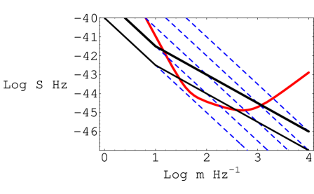
The above results, to be interpreted only as a first qualitative indication, are confirmed by a more realistic analysis of the cross correlation of the two LIGO interferometers [318], performed by applying Eq. (6.56) to the phenomenological power spectrum:
| (6.60) |
In spite of the reduced value of the overlap factor we find (for any , but with ) a significant SNR in the relevant mass range, already at the level of the Enhanced LIGO configuration. No possibility of detection, even with the Advanced LIGO configuration, is found instead for a non-relativistic spectrum peaked outside the detector sensitivity band, such as the “minimal” spectral distribution (6.12), (6.13). It should be stressed, however, that interferometric detectors are particularly unfavoured for the detection of a non-relativistic scalar background, because their response tensor is traceless: spherical resonant detectors represent more promising devices, and it seems appropriate to conclude this section by reporting the possible enhanced level of SNR when a massive scalar background interacts with the monopole mode of a resonant sphere [175].
For a massive scalar wave there are in fact two possible pattern functions, one associated to the geodesic coupling of the detector to the scalar component of metric fluctuations [465] (the Riemann term in Eq. (6.20)), the other related to the direct, non-geodesic coupling of the charge of the detector to the spatial gradients of the scalar background [286]. In terms of the transverse and longitudinal decomposition of the polarization tensor of the wave, with respect to the propagation direction ,
| (6.61) |
the two pattern functions can be written, respectively, as [318]
| (6.62) |
For the differential mode of an interferometer [256] , so that, in both cases, the pattern function of massive waves turns out to be proportional to the massless pattern function and, for non-relativistic modes, it is highly suppressed by the factor [318]. The monopole mode of a resonant sphere, on the contrary, is characterized by the response tensor [83]. The non-geodesic pattern function is still suppressed, but the geodesic part is not, and the overlap function (6.57) takes the simple form
| (6.63) |
where is the spatial separation of the detectors. The response to scalar spectra peaked at is thus strongly enhaced with respect to interferometric detectors (at least in the case of geodesic coupling).
Beside this effect there is a second possible enhancement, for flat enough spectra, associated to a faster growth of SNR with the observation time . Consider, for instance, the cross-correlation of two spherical detectors according to Eq. (6.56), computed for the spectrum (6.60) with the overlap (6.63). Assuming that the instrumental noises are constant (and finite) for ranging from to , it follows that for the momentum integral is dominated by its lower limit, i.e. by the infrared cut-off scale determined, for , by the “minimum” observable frequency interval associated to the “maximal” observation time [175]:
| (6.64) |
This effect modifies, for , the final -dependence of SNR, and enhances the response of the detector with the growth of the observation time. Performing the integral for one finds in fact (modulo numerical factors)
| (6.65) |
to be compared with the more standard result
| (6.66) |
For s, and a mass in the kilohertz range, the sensitivity of spheres to a flat enough and massive spectra is thus increased by a factor with respect to interferometric detectors (see [175] for a more detailed discussion).
We may thus conclude, summarizing the results of this subsection, that both interferometric and resonant gravitational antennas seem to be able to explore the possible presence of a light (but non-relativistic) dilatonic component of dark matter, and thus to constrain the parameters of the pre-big bang models, in a mass range that overlaps with their sensitivity band. This is possible in spite of the fact that the relic dilaton background could be directly coupled to the total mass of the detector, with a charge that is much weaker than gravitational. Spherical detectors are more efficiently coupled to massive scalar waves, but enhanced and advanced interferometers are already sufficient to provide significant constraints on a possible background of relic dilatons.
7 Relic photons, axions and CMB anisotropy
As discussed in the previous sections, the primordial spectrum of (scalar and tensor) metric fluctuations, amplified by a phase of pre-big bang inflation, is characterized in general by a positive and rather steep slope. Because of the high-frequency normalization of the peak of the spectrum, controlled by the string scale, the amplitude of metric fluctuations is strongly suppressed at the large-distance scales relevant to the anisotropy of the CMB radiation observed by COBE [568, 78], or to the density fluctuations spectrum (see for instance [510]) required by the standard mechanism of structure formation. It thus seems difficult, in such a context, to generate a flat spectrum of scalar curvature perturbations directly responsible for the above effects, unless we accept rather drastic modifications of the pre-big bang kinematics, as recently suggested in [252, 228] (and briefly discussed in Subsection 7.2).
The slope of the spectrum, however, depends on the external “pump” field, which amplifies the quantum fluctuations (see Section 4) and which contains, in general, the contribution of all the components of the background (metric, dilaton, moduli fields, …). Different fluctuations are coupled to different pump fields and may have very different spectra, even in the same background.
It turns out, in particular, that the primordial spectrum of electromagnetic [306, 307] and of “axionic” [176, 183] fluctuations (i.e. the fluctuations of the four-dimensional NS-NS two-form and of other, string- and M-theory-motivated, antisymmetric tensors) may be characterized by a slope much flatter than the slope of the metric perturbation spectrum (in some cases, even decreasing [136, 185, 120, 332, 227], depending on the coupling to the moduli fields, on the anisotropy of space-time, and on the number of extra dimensions). A flat and primordial distribution of (isocurvature) axionic fluctuations, in turn, can directly generate a scale-invariant spectrum of CMB anisotropies through the “seed” mechanism [224, 225, 325], which will be reported in Subsections 7.3, 7.4, or even generate an adiabatic, scale-invariant spectrum of density and curvature perturbations through the “curvaton” mechanism recently discussed in [242, 460, 488, 66, 503, 489, 101], and illustrated in Subsection 7.5.
In addition, the amplification of electromagnetic fluctuations, with a flat enough spectrum, seems to naturally provide the seed fields required to explain the origin of the magnetic fields present on a galactic and intergalactic scale (see [346] for a recent review). We will first illustrate this interesting possibility in the next subsection.
7.1 Large-scale magnetic fields and photon production
In the context of the pre-big bang scenario, the background evolution that amplifies metric perturbations also amplifies the quantum fluctuation of the electromagnetic field, because of their direct coupling to the dilaton and to the moduli fields. For the heterotic string model, such a coupling is described by the effective action [306]
| (7.1) |
where controls the tree-level four-dimensional gauge coupling ( being the ten-dimensional dilaton field, and the volume of the six-dimensional compact internal space). The effective coupling to the external geometry may be different, however, if the electromagnetic symmetry is a component of the Kaluza–Klein gauge group produced in the compactification down to dimensions [136] (see also [336]).
The electromagnetic field is also coupled to the four-dimensional geometry, of course. If such a coupling is minimal, however, it is also conformally invariant, and therefore does not contributes to photon production in a conformally flat metric such as that of a typical inflationary background, unless conformal invariance is broken at the classical [590] or quantum [219] level. Even in that case, however, photon production turns out to be rather suppressed (with respect to graviton production, for instance).
In order to discuss the amplification induced by the dilaton, in a conformally flat metric , it is convenient to use the radiation gauge , explicitly. Because of conformal invariance, the coupling to the metric disappears from the action (7.1); after partial integration the action becomes, in this gauge,
| (7.2) |
and can be easily diagonalized by setting
| (7.3) |
For each polarization mode we then obtain the effective action
| (7.4) |
and the canonical evolution equation
| (7.5) |
which is exactly the same as the graviton equation (4.56), with the only difference that now the pump field is fully determined by the dilaton. If we use, in particular, the minimal model of background introduced in Subsection 5.2, the spectrum of the amplified electromagnetic fluctuations will be characterized by the same parameters as the graviton spectrum. In such a case, the constraints on the electromagnetic spectrum will provide constraints on the parameters of the model and then, indirectly, on the associated graviton spectrum.
An important application of the “dilatonic” amplification of the electromagnetic fluctuations is the possible production of “seed” for the galactic magnetic fields [306, 431]. The origin of the large-scale cosmic magnetic fields (with coherence scale kpc, and typical amplitude G) is in fact, to a large extent, still an open problem [346]. Almost all mechanisms invoked to generate the large-scale fields, e.g. the galactic “dynamo” [509, 633], require the presence of small, primordial seeds to trigger the subsequent magnetic amplification. Many mechanisms of seed production have been suggested [366, 590, 596, 533, 264, 219, 158, 415] [82, 125, 339, 186] [68, 253, 202, 472, 292], trying to bypass the difficulty –due to conformal invariance– that forbids a standard inflationary amplification of the electromagnetic fluctuations. In the context of the pre-big bang models, on the contrary, the seeds can be produced directly from the electromagnetic fluctuations of the vacuum, thanks to the accelerated growth of the dilaton during the pre-big bang phase (with possible additional contributions from dilaton oscillations, during preheating [329]).
Consider in fact the two-parameter model of Eqs. (5.10):
| (7.6) |
The effective dilatonic potential of Eq. (7.5) grows during the dilaton phase, keeps growing during the string phase, and goes to zero in the radiation era. Because of the two background transitions, there are two bands of the spectrum, corresponding to modes hitting the barrier in the dilaton phase, , and in the string phase, . By applying the standard procedure of Subsection 4.4 we obtain:
| (7.7) | |||||
where . By recalling that (see Eq. (5.14)), we find that the electromagnetic spectrum thus has the same parameters as the graviton spectrum (5.15), but the slope is in general flatter. Even flatter spectra are possible for vector fields of Kaluza–Klein origin [136].
The generation of fluctuations of a strength large enough to seed the galactic dynamo constrain the electromagnetic spectrum at the megaparsec scale, and imposes in particular a bound that, in the most conservative form, can be written as follows [590]:
| (7.8) |
where is the epoch of galaxy formation, i.e. . Remarkably, this condition is compatible with the condition of negligible backreaction,
| (7.9) |
(at all frequency scales), required by the consistency of the perturbative approach around a homogeneous unperturbed background.
There is indeed a wide region of parameter space in which the two conditions are consistent without fine-tuning [306], as illustrated by the shaded and hatched areas of Fig. 7.1 (the hatched area refers to the dilaton branch of the spectrum, ; the shaded area to the string branch, ). As shown in the picture, the production of seeds is strong enough to satisfy the needs of the dynamo mechanism (Eq. (7.8)), provided the coupling is sufficiently small at the beginning of the string phase:
| (7.10) |
and the duration in time of the string phase is sufficiently long:
| (7.11) |
(in cosmic time, ). For illustrative purposes, the plots of Fig. 7.1 have been constructed by taking as a reference value. We also note that, besides the condition (7.9), there are additional bounds on the energy spectrum of the magnetic fields because of a possible (classical) production of gravitational waves induced by the magnetic stress tensor [145]. Flat enough spectra are not strongly constrained, however, and we are assuming that this is indeed the case for the electromagnetic distribution that we are considering. Possible additional bounds on the primodial magnetic amplitude, due to Faraday rotation effects, may follow in principle from future measurements of the CMB polarization, as discussed in [330].
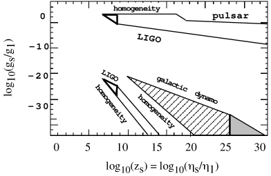
Also shown in Fig. 7.1 are the allowed regions of parameter space compatible with the detection of the relic graviton background produced in the context of minimal pre-big bang models. We have used the typical sensitivity expected for the cross-correlation of two second-generation interferometers, with the characteristic of Advanced LIGO (see Eq. (5.42)). The allowed region is then defined by the condition , imposed on the spectrum (5.15), together with the pulsar bound (5.3), and the condition of negligible backreaction ( at all and ), required for the validity of our perturbative computation of the spectrum around a homogeneous background (for a detailed implementation of all bounds see [275]). It turns out that there are two allowed regions, corresponding to tensor perturbations whose comoving amplitude stays constant outside the horizon during the string phase (upper region) or grows (lower region). At the left-end of each region, the marked triangular area corresponds to the possible detection of low-energy modes, crossing the horizon during the dilaton-dominated phase; the rest of the allowed region refers to modes crossing the horizon during the string phase.
It should be noted that the gravitationally allowed regions have no possible overlap with the electromagnetic ones, implying that the interesting phenomenological possibilities of seed production and of graviton detection tend to exclude each other [275]. Indeed, if we restrict to the class of backgrounds consistent with the production of magnetic seeds (i.e. inside the shaded and hatched regions of Fig. 7.1), then the allowed slope of the high-frequency (string) branch of the graviton spectrum is constrained to vary between and [279], with a consequent drastic reduction of the allowed region for , as illustrated in Fig. 7.2. In that case, the graviton background is certainly outside the range of currently available detectors (resonant bars and ground-based interferometers), which reach their maximal sensitivity in the frequency band – Hz.
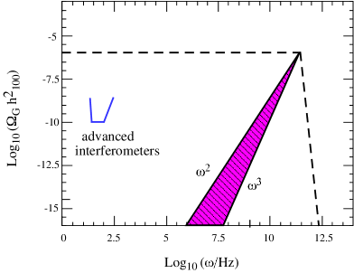
According to the above analysis, a future detection of cosmic gravitons in the hertz to kilohertz range would seem to exclude a dilatonic origin of the seed magnetic fields, directly amplified from the fluctuations of the vacuum. Conversely, an absence of signals from the relic graviton background would seem to support, indirectly, a primordial dilatonic origin of the cosmic magnetic fields. It must be stressed, however, that such conclusions, based on the plots of Fig. 7.1, cannot be applied in general to the pre-big bang scenario: they are only pertinent to the class of minimal models introduced in Subsection 5.2, and could be evaded in the context of more complicated models of background.
A final remark concerns the fact that the photon spectrum (7.7) is in general flatter than the graviton spectrum (5.15), suggesting the possibility that the electromagnetic fluctuations may also act as seeds for the (approximately) scale-invariant spectrum of temperature anisotropies of the CMB radiation [307, 276] and for the density perturbations required for the structure formation. According to a detailed analysis [225], however, such a possibility has to be discarded in favour of an analogous possibility based on the fluctuations of the fundamental antisymmetric tensors appearing in the bosonic sector of string theory, which can be amplified with a perfectly flat spectrum [176, 183], as will be illustrated in the next subsection.
7.2 Large-scale CMB anisotropy and axion production
In the context of the standard inflationary scenario, the observed CMB anisotropy, at very large angular scales, can be consistently generated by the primordial spectrum of scalar metric fluctuations through the Sachs–Wolfe (SW) effect [547], . Indeed, when the metric fluctuations are directly amplified by the accelerated evolution of the background, their spectral distribution is controlled by the value of the Hubble scale at the time of horizon crossing, . For a standard de Sitter (or quasi-de Sitter) inflationary solution, is constant in time, so that the spectrum is scale-invariant. A typical normalization of the spectrum, corresponding to inflation occurring roughly at the GUT scale [423],
| (7.12) |
is thus perfectly consistent with the anisotropy observed at the present horizon scale [568, 78], , and with the fact that the spectrum is scale-invariant.
In the context of the pre-big bang scenario, on the contrary, the curvature scale grows with time, so that the spectrum of the metric fluctuations tends to grow with frequency, as illustrated in Section 4. In addition, the natural inflation scale corresponds to the string scale, so that the normalization of the spectrum, at the end-point frequency , is controlled by the ratio
| (7.13) |
As a consequence, for a typical pre-big bang model, the slope of the spectrum is too steep, and the normalization too high, to be compatible with the COBE observations. The slope is so steep, however, that the contribution of the metric fluctuations to is certainly negligible at the COBE scale. So, on the one hand there is no contradiction with observations, namely the COBE data cannot be used to rule out pre-big bang models [284]. On the other hand, the problem remains: How to explain the observed CMB anisotropy?
There are two possible answers to this question. The first one relies on somewhat drastic modifications of the kinematics of the pre-big bang phase illustrated in the previous sections, in such a way as to generate a primordial scale-invariant spectrum directly from the amplification of the vacuum fluctuations of the metric, as in the standard inflationary scenario. The second possibility relies on the indirect generation of scale-invariant metric perturbations through the isocurvature fluctuations of another field, which may have a flat spectrum even in the context of the pre-big bang solutions illustrated up to now in this paper. We will discuss in detail the second possibility in the following subsections. Here we will briefly report on the first possibility.
There are at present two possible examples of pre-big bang models characterized by a flat primordial spectrum of scalar perturbations [252, 228]. They are both based on the introduction of a negative, exponential dilaton potential , which can be parametrized in the E-frame as follows (in units ):
| (7.14) |
and which is similar to the attractive potential existing between the colliding branes in the context of the ekpyrotic scenario [413, 414].
With such a potential, the corresponding (E-frame) pre-big bang solution describes an accelerated contraction, controlled by the dimensionless parameter ,
| (7.15) |
which has to match the subsequent phase of decelerated, radiation-dominated expansion. By assuming the existence of a non-singular bounce for the background solution, and assuming the continuity of the Bardeen potential and of the curvature perturbation across the bounce (their continuity is guaranteed by performing the matching on the constant density hypersurface), one then finds that after the bounce the spectrum of is determined by the pump field (7.15), according to the rules derived in Section 4, namely
| (7.16) |
A flat spectrum of scalar perturbations can then be obtained for , as noted in [252], corresponding to a dilaton potential that simulates a “dust” matter source with vanishing effective pressure .
Alternatively, as recently discussed in [228], a flat spectrum of scalar metric perturbations can be obtained from the background solution (7.15) by assuming a very slow contraction, i.e. as in the ekpyrotic scenario [413, 414], and assuming that the matching to the expanding phase is performed across a hypersurface different from that of constant energy density (for instance, across the zero-shear hypersurface [228]). In that case the scalar spectrum after the bounce turns out to be different from Eq. (7.16), and is given by
| (7.17) |
The case thus reproduces a (nearly) flat spectrum, for both the pre-big bang and ekpyrotic scenarios.
This result can be easily explained by noting that, in the transition from a contracting to an expanding phase, the asymptotic solutions of the scalar perturbation equations are a linear combination of a constant and of a growing mode before the transition, and of a constant and a decaying mode after it. Consider, for instance, a bouncing background evolving from the contracting solution (7.15) valid for , to the standard, radiation-dominated expansion , valid for . The asymptotic solutions for the super-horizon modes of the Bardeen potential, in the longitudinal gauge, can be written as
| (7.18) |
where , and . Here are determined by the initial normalization to a vacuum fluctuation spectrum, while are to be determined by the matching conditions. It is then clear that different matching prescriptions may lead to different solutions for , the dominant mode of the post-big bang expanding phase, and then to different final spectra.
Given a space-like hypersurface, with normal vector , the matching of two background manifolds [387] has to be performed on the induced metric and on the extrinsic curvature of the given hypersurface, where
| (7.19) |
For the given example of bouncing background the metric will be continuous, i.e. , where
| (7.20) |
the curvature, however, will be characterized by a “jump” from negative to positive values, (if we neglect the high-energy corrections, which are expected to smooth out the singularity, see Section 8). This introduces in general a surface stress tensor, which in our case corresponds to a tension (i.e. to a negative pressure), needed to avoid the singularity and to implement the transition from contraction to expansion.
The matching of the metric fluctuations can now be performed by perturbing the Israel junction conditions on the chosen hypersurface, and leads to
| (7.21) |
On a general hypersurface one then obtains that the dominant coefficient , determining the post-big bang asymptotic expansion of the Bardeen potential, is in general related to the pre-big bang coefficients by [228]
| (7.22) |
where are (possibly -dependent) coefficients, and represents the perturbation of the surface tension. The final spectrum thus depends, in general, not only on the choice of the matching hypersurface, but also on its perturbed tension (i.e. on the details of the regularizing mechanism that is responsible for the bouncing transition).
The matching across the hypersurface of total constant energy density ( const) gives in particular [228] so that, assuming a negligible , simply inherits the spectrum of the constant mode , and one is led to the “standard” result (7.16) for the scalar perturbation spectrum. The matching across a different hypersurface leaves, however, , so that the final spectrum is dominated by the growing mode of the pre-big bang solution and (again assuming a negligible ) one is led to the “new” result reported in Eq. (7.17), which leads to a flat spectrum for all backgrounds with .
In the rest of this section we will adhere, however, to the standard matching prescription at constant energy density, and we will concentrate on the alternative possibility of an indirect generation of scale-invariant metric perturbations through the fluctuations of another background field. Such an auxiliary field, in a string cosmology context, can be naturally identified with the axion, whose quantum fluctuations, unlike the metric fluctuations, can be directly amplified with a flat spectrum, even in the context of the minimal pre-big bang models (without the contribution of a dilaton potential).
To explain the reason of such a difference, first pointed out in [176, 183], let us consider the four-dimensional reduced action for the antisymmetric tensor ,
| (7.23) |
where
| (7.24) |
The equation of motion,
| (7.25) |
can be automatically satisfied by introducing the “dual” axion field :
| (7.26) |
( is the totally antisymmetric, covariant tensor), and the effective action (7.23) may be rewritten
| (7.27) |
(note the coupling of to instead of ). In conformal time, and for a conformally flat metric
| (7.28) |
the action can be diagonalized by setting
| (7.29) |
so that the evolution equation for the axion canonical variable is formally the same,
| (7.30) |
but is characterized by a pump field different from that of gravitons or photons. Assuming a smooth evolution from a power-law pre-big bang background, with , to the standard radiation era, the axion spectrum is then determined by the background kinematics according to the general prescriptions of Subsection 4.4, i.e.
| (7.31) |
Consider now the low-energy branch of the spectrum, for modes hitting the effective potential barrier during a higher-dimensional dilaton-driven phase, which we assume to be characterized by three isotropically expanding dimensions, with scale factor , and “internal” dimensions, with scale factor . The background evolution is known, determined by the , anisotropic, S-frame solutions of the string effective action, Eqs. (2.88) and (2.89). The scale factors, and the dimensionally reduced dilaton , can then be expressed in conformal time as
| (7.32) |
where are parameters related by the “Kasner-like” condition
| (7.33) |
( for inflationary expansion), and is the dilaton field appearing in the -dimensional, non-reduced action,
| (7.34) |
Combining the behaviour of and we obtain the power of the pump field, and the corresponding spectral index, which are in general given by :
| (7.35) |
In the particular case of an isotropic -dimensional subspace, , , one can also re-express the spectral index (7.35) in terms of the conformal power of the modulus, as originally done in [176], or even in terms of a parameter , measuring the relative evolution in time of the external and internal volumes [480]. What is important, in our context, is that a flat spectrum (i.e. const, ) is now perfectly allowed for . For an isotropic -dimensional background, in particular, , so that a flat spectrum exactly corresponds to , i.e. just the number of dimensions of critical superstring theory! (see also [136]). Flat (or nearly flat) spectra are also possible for different exact solutions of the low-energy string effective action [178, 179, 325], even in four dimensions if the background is anisotropic [332], or if the dilaton has an appropriate exponential potential and it is non-minimally coupled to the axion [252].
It should be stressed that for gravitons, on the contrary, a flat spectrum cannot be obtained in the above background, quite irrespective of the number and dynamics of the internal dimensions. By using Eq. (7.32) we find indeed that, independently of , the graviton pump field always has the same power, ,
| (7.36) |
so that the spectrum (modulo logarithmic corrections) is always characterized by the known cubic slope . A flat spectrum, in the background (7.32), is also forbidden for heterotic photons (coupled to the dilaton as in the example discussed in the previous subsection). The situation is different, however, for Kaluza–Klein photons, whose spectrum is more sensitive to the dynamics of the internal dimensions [136].
It is important to note, finally, that in the different backgrounds obtained through transformations mixing the axion and dilaton fields, different evolution equations are generally obtained for the metric, the dilaton, and the axion fluctuations. After a diagonalization, and a redefinition of new canonical variables, one finds however that the evolution equations for the two fundamental scalar degrees of freedom, i.e. the gauge-invariant (Bardeen) potential and the pseudoscalar axion field, are unaltered by the transformation. Thus, the blue spectral tilt of metric perturbations and a possibly flat slope of the axion spectrum remain the same as in the standard, dilaton-dominated background solutions [176, 183] (see also [438] for more details on the axion spectra).
A flat, primordial spectrum of axion fluctuations can be used for an indirect generation of the observed CMB anisotropies in two ways. A first possibility is the “seed” mechanism [221, 222]: indeed, even if the axion fluctuations are negligible as sources of the metric background, , their inhomogeneous stress tensor generates metric fluctuations according to the standard gravitational equations, and the metric, in its turn, is source of the temperature anisotropies through the usual Sachs–Wolfe effect:
| (7.37) |
Such an indirect production of anisotropies could work, in principle, because the contribution (7.37) to is quadratic in the axion field, and not linear as in the case of metric perturbations. So, even if the amplitude of the axion fluctuations is still normalized at the string curvature scale, the square of the amplitude is not very far from the expected value :
| (7.38) |
The string normalization (7.13), on the other hand, is imposed at the end point of the spectrum (typically, at the gigahertz scale), while COBE observations constrain the spectrum at the present horizon scale ( Hz): it is then evident that a very small, “blue” tilt in the axion spectrum is sufficient to make compatible the string and COBE normalizations, Eqs. (7.38) and (7.12).
The seed mechanism, however, seems to have difficulties in reproducing the peak structure of the observed anisotropies at smaller angular scales, as will be discussed in Subsection 7.3. A more realistic scenario is probably offered by the “curvaton” mechanism [460]: if the axion is heavy enough, the initial and flat primordial spectrum of isocurvature axion fluctuations can be eventually converted, after the axion decay, into a final scale-invariant spectrum of curvature fluctuations. The standard results for the temperature anisotropies then apply, with the only difference that the metric perturbations are not primordial, but indirectly generated by the axion decay. This possibility will be discussed in Subsection 7.5, after a brief report on the seed mechanism, which will be presented in the next two subsections.
7.3 Massless axions as seeds
The quantum fluctuations of the so-called “universal” (or Kalb-Ramond) axion (i.e. the dual of the field strength of the NS-NS two-form appearing in the string effective action) can be amplified with a scale-invariant distribution of the spectral energy density, (as shown in the previous subsection); they are thus a possible candidate for seeding the large-scale anisotropy in the context of the pre-big bang scenario. To illustrate this possibility we will proceed in two steps.
We will first show that the scalar metric fluctuation on a given scale , at the time the scale re-enters the horizon, is precisely determined by the axion energy distribution evaluated at the conformal time of re-entry, :
| (7.39) |
Secondly, we will show that the dominant contribution of a given scale to the Sachs–Wolfe effect comes from the time that scale re-enters the horizon, in such a way that the final temperature spectrum exactly reproduces the primordial seed spectrum:
| (7.40) |
These two results are far from being trivial, as they are consequences of the particular time dependence of the Bardeen spectrum induced by axion fluctuations (the same results do not apply, for instance, to the case of electromagnetic fluctuations). We will give here only a sketch of the arguments leading to the above results, which are interesting in themselves, apart from their possible string cosmology applications. For a detailed derivation we refer the reader to the original papers [224, 225].
Let us first compute the spectrum of metric perturbations seeded by a flat, primordial distribution of axion fluctuations. We define, as usual, the power spectrum of the Bardeen potential, , in terms of the Fourier transform of the two-point correlation function,
| (7.41) |
(the brackets denote spatial average, or expectation value if perturbations are quantized), and we recall that the square root of this function, evaluated at a comoving distance , represents the typical amplitude of fluctuations on a scale :
| (7.42) |
(see also Eq. (4.69)). We also define the power spectrum of the seed stress tensor, in the same way (no sum over , ):
| (7.43) |
Metric fluctuations and seed fluctuations, on the other hand, are related by the cosmological perturbation equations [222]. By taking into account the important contribution of the off-diagonal components of the axion stress tensor one finds, typically, that the Bardeen spectrum and axion energy–density spectrum are related by:
| (7.44) |
where , and
| (7.45) | |||||
Note that the two-point correlation function of the energy density becomes a four-point function of the seed field, since the energy is quadratic in the axion field.
Using now the stochastic average condition for the axion field,
| (7.46) |
it turns out that the energy–density spectrum reduces to a convolution of Fourier transforms,
| (7.47) |
Also, for a flat enough axion spectrum, one finds that the above integral is dominated by the region [225]. By expressing the convolution through the spectral energy density , evaluating the Bardeen potential at the time of re-entry , and using Eq. (7.44), one is finally led to relating the Bardeen spectrum and the axion spectrum as follows:
| (7.48) |
We should now explain why we are interested in the metric fluctuations evaluated at the time of re-entry.
To this purpose, let us compute the seed contribution to . In the multipole expansion of the temperature anisotropies (in terms of the Legendre polynomials ),
| (7.49) |
the coefficients , at very large angular scales (), are determined by the Sachs–Wolfe effect as [222]:
| (7.50) |
Here and are the two independent components of the gauge-invariant Bardeen potential (see Subsection 4.2), are the spherical Bessel functions, and a prime denotes the derivative with respect to their argument. Equation (7.50) takes into account both the “ordinary” and the “integrated” Sachs–Wolfe contribution, namely the complete distortion of the geodesics of the CMB photons (due to shifts in the gravitational potential), from the time of decoupling down to the present time . By inserting the Bardeen potential determined by the axion field, we find that the time-integral is dominated by the region . Using Eq. (7.48) we finally obtain
| (7.51) |
which gives the multipole coefficients in terms of the axion distribution , through Eq. (7.48). This explains why it was important to evaluate the Bardeen spectrum at the time of re-entry, .
From this final expression we can extract, in particular, the value of the quadrupole coefficient [225]:
| (7.52) |
where is the spectral index (sufficiently near to ) characterizing the primordial axion distribution, is the comoving scale of the present horizon, and the end point of the spectrum, namely the maximal amplified comoving frequency. We have assumed, in the context of a minimal model of pre-big bang, that the peak amplitude of the axion spectrum, at the end-point frequency, is controlled by the fundamental ratio between string and Planck masses, as it was for the graviton and dilaton spectra computed in the previous sections. Note, however, that in the low-frequency band corresponding to the large-scale observations the axion spectrum contains the enhancement factor (see Eq. (5.2)), which for almost exactly cancels the present radiation energy density, .
The quadrupole coefficient, on the other hand, is at present determined by COBE as [51]
| (7.53) |
This experimental value, inserted into Eq. (7.52), provides an interesting, direct relation between the string mass and the spectral index of the temperature anisotropy. Using (see Eq. (5.16)), and using (as a reference value) the following bounds on the spectral index [79]:
| (7.54) |
(we have excluded here the allowed values , to avoid introducing an infrared cut-off in the massless axion spectrum), we obtain in fact an allowed range for the string-mass scale, , which is compatible with the theoretical expectations [404], . Conversely, the theoretically expected range for implies a spectral index , which is also in agreement with the observational results.
This promising result, however, is only a first step towards a more complete comparison of the seed model with observations, comparison that must include also smaller angular scales, where precise experimental data have recently been obtained [484, 476, 204, 364], and will become available in the next few years [471, 522].
A numerical computation of the anisotropy power spectrum (7.50), at intermediate angular scales (up to ), has already been performed as reported in [480, 609]. The resulting spectrum shows the familiar peak structure, typical of all inflationary models. However, as was already shown very clearly by a first analysis [480], the height and the position of the first acoustic peak can be reproduced (at least approximately) only if the axion spectrum grows fast enough with frequency. In particular, using the notation of the previous subsection, one must require at least (but seems to be favoured by the data).
This requirement, however, is in general incompatible with the high-frequency normalization typical of the pre-big bang scenario (if the amplitude is large enough to match observations at the COBE scale and the slope is too steep, then the energy density blows up and becomes overcritical at the string scale).
A possible solution, suggested in [480], exists in the context of “non-minimal” models of background, leading to a slope that is steep enough at low frequency, and flatter at high frequency, so as it limits the peak value. Since the axion spectrum depends both on the number and on the kinematics of the internal dimensions (see Subsection 7.2), such a spectrum could be produced during a phase of dynamical dimensional reduction, in which the low-frequency modes are frozen outside the horizon while the Universe is dimensionally different from the subsequent phase of freezing of the high-frequency modes.
A more detailed analysis [609], based on the recent BOOMERanG-98 [204] and MAXIMA-1 [364] data, shows indeed that it is not impossible to fit the height of the first acoustic peak, observed around , by using a (pre-big bang-motivated) axion spectrum, which grows with a steep slope up to a limiting scale , and which is pretty flat above :
| (7.55) |
In order to be efficient, the break point has to be around the equilibrium scale, . However, the precise position of the break is not strongly constrained, and one may exploit the possibility of lowering the break scale, to lower the height of the second (and subsequent) acoustic peaks, for a better comparison with data (such a shift does not substantially affect the height of the first peak).
A break in the axion spectrum is thus effective to match the height of the peaks, but is not sufficient to fit the position of the first acoustic peak, determined with small uncertainty by recent data [484, 476, 204, 364] around . The position depends on the full set of parameters of a given cosmological model and, in the context of the seed mechanism based on massless axions, a peak at seems to require a moderately closed Universe , with . For instance [609],
| (7.56) |
provides a good fit of the data, also compatible with current supernovae results [518]. It should be noted, to confirm the validity of a such model, that if the axion spectrum has a break it is also possible to fit the dark-matter power spectrum, in reasonable agreement with observations.
However, even adjusting the break point and the value of , the width of the peak is still not in very good agreement with the present data, as the resulting normalized is about , which confirms the model only at the % confidence level [609]. Nonetheless, it is important to stress that the position of the second acoustic peak predicted by the axion model is different from the one indicated by the standard inflationary predictions (and by present data). In addition, the axion model also predicts a small peak, or “hump”, around , due to the “isocurvature” (rather than adiabatic, i.e. isoentropic) nature of the induced metric perturbations. These two peculiar predictions will be extremely important to confirm or disprove definitely the axion model, when the future satellite observations [471, 522] will become available.
Also, the axion fluctuations are described by a Gaussian, stochastic variable, but the induced metric fluctuations depend on the axion energy–momentum tensor: they are quadratic in and therefore non-Gaussian, in general. This may change the estimate of the confidence level (i.e. of the probability) that the axion model leads to the measured CMB anisotropy spectrum.
It should be stressed, to conclude this subsection, that the isocurvature character of the primordial axion spectrum considered here is due to the fact that the axions are treated as seeds, i.e. inhomogeneous fluctuations of a background that is not axion-dominated. As a consequence, the predicted anisotropies are different from previous models of isocurvature axion perturbations [43, 559, 497]. So, even if this seed mechanism based on isocurvature axion perturbations were definitely ruled out by future observations, this would not preclude the possibility of adiabatic axion perturbations (see for instance [410]), where the axions produced during the phase of pre-big bang inflation represent a significant fraction of the present cold dark-matter density.
7.4 Massive axion spectra
In the previous subsection we have discussed the CMB anisotropies seeded by a stochastic background of massless axion fluctuations, amplified by a phase of pre-big bang inflation. It is possible, or even likely, however, that the axion fluctuations amplified by inflation become massive in the post-inflationary era: it is thus important, also in view of future applications other than the seed mechanism, to discuss whether, even in the massive case, the string normalization of the primordial spectrum may be consistent with the large-scale normalization determined by the CMB anisotropy, in spite of some important differences that appear in the spectrum and in the computation of the Sachs–Wolfe effect.
In this subsection we shall keep assuming that the axion background is negligible, , and that the whole contribution to the axion energy density comes from the vacuum fluctuations, as in the previous subsection. There are, however, various important differences. A first difference between the massless and massive axion cases concerns the relation between and the Bardeen potential . In the massless case the perturbation equations, taking into account the important contribution of all the off-diagonal terms of the axion stress tensor, lead to
| (7.57) |
(see Eq. (7.44)). In the massive case, on the contrary, the axion stress tensor can be approximated as a diagonal, perfect-fluid stress tensor, and we obtain [325]
| (7.58) |
Also, the convolution (7.47) for the axion energy density is dominated by the region in the massless case, and by in the massive case. In the massless case the integrated Sachs–Wolfe effect is dominant, while it is the ordinary one that dominates in the massive case [325].
In spite of these differences, the final result for the temperature anisotropies is the same as before, with the quadrupole coefficient determined by the axion spectral energy density as [325]
| (7.59) |
In the massive case, however, the axion spectrum is affected by non-relativistic corrections, which are to be computed by including the mass contribution to the canonical evolution equation (7.30):
| (7.60) |
To this purpose, let us consider a simple background transition at , from an initial pre-big bang phase in which the axion is massless, to a final radiation-dominated phase in which the dilaton freezes to its present value, const, and the axion acquires a mass, which is small in string units. Therefore, for , we then have , and the usual Hankel solution is normalized to a vacuum fluctuation spectrum (see Section 4.4),
| (7.61) |
where depends on the pre-big bang evolution of the pump field . In the subsequent radiation era, , the effective potential is vanishing, and the perturbation equation reduces to
| (7.62) |
where we have put
| (7.63) |
using the time behaviour of the scale factor .
For the high-frequency modes that are relativistic at the transition scale, , the mass term can be neglected, and we can match the solution (7.61) to the plane-wave solution
| (7.64) |
to obtain:
| (7.65) |
(we neglect, for simplicity, numerical factors of order , which will be absorbed into the uncertainty relative to the inflation scale, represented by the overall numerical coefficient in front of the final spectrum.) In the relativistic regime the amplified axion perturbation then takes the form:
| (7.66) |
and the corresponding energy density, , integrated over all modes, leads to the spectral distribution (4.102), and to the usual relativistic spectrum (normalized to critical units):
| (7.67) |
where is the proper momentum (see Subsection 4.4).
In the radiation era the proper momentum is redshifted with respect to the rest mass, and all axion modes tend to become non-relativistic. When the mass term is no longer negligible, on the other hand, the general solution of Eq. (7.62) can be written in terms of parabolic cylinder functions [6]. For an approximate estimate of the axion field in the non-relativistic regime, however, it is convenient to distinguish two cases, depending on whether a mode becomes non-relativistic inside or outside the horizon. Defining as the limiting comoving frequency of a mode that becomes non-relativistic () at the time it re-enters the horizon (), we find, in the radiation era [325],
| (7.68) |
We will consider the two cases and separately.
In the first case we can rewrite Eq. (7.62) as
| (7.69) |
and the general solution we give has the form
| (7.70) |
where are the Weber parabolic cylinder functions (see [6], Chap. 19). In order to fix the integration constants and we can match the solutions (7.70) and (7.66) in the relativistic limit where
| (7.71) |
In this limit, since we are considering modes that become non-relativistic when they are already inside the horizon,
| (7.72) |
we can expand the functions for large with moderate [6]. Matching to the plane-wave solution (7.64), we obtain , and
| (7.73) |
In the opposite, non-relativistic limit , the expansion of the Weber functions gives [6]
| (7.74) |
(we have used ). The corresponding axion field is then (inside the horizon)
| (7.75) |
The associated energy density, , differs from the previous one by the non-relativistic rescaling , thus leading to the spectrum
| (7.76) |
where (see Eq. (7.67)).
Finally, we consider the case of a mode that becomes non-relativistic when it is still outside the horizon, . In this case, we cannot use the large expansion as , and it is convenient to express the general solution of Eq. (7.69) in the form
| (7.77) |
where and are the even and odd parts of the parabolic cylinder functions [6]. The matching to (7.66), in the relativistic limit , gives and
| (7.78) |
In the non-relativistic limit we use the relation [6]
| (7.79) |
which leads to
| (7.80) |
from which
| (7.81) |
with an associated spectrum
| (7.82) |
reproducing the low frequency band of the non-relativistic spectrum already presented in the case of dilatons (see Eq. (6.13)).
However, the above result is valid only if the axion field becomes massive before the limiting scale crosses the horizon. Let us call the temperature scale at which the mass turns on (typically, MeV if axions become massive at the epoch of chiral symmetry breaking) and the proper frequency re-entering the horizon precisely at the same epoch. The present value of is then
| (7.83) |
and the spectrum (7.82) is valid for , namely for . In the opposite case, , the role of the transition frequency, which separates modes that become non-relativistic inside and outside the horizon, is played by , and the lowest-frequency band of the non-relativistic spectrum (7.82) has to be replaced by [325]:
| (7.84) |
(such a spectrum can be easily obtained by imposing the continuity with (7.76) at ).
In both cases, as clearly illustrated in Fig. 7.3, the effect of non-relativistic corrections is to enhance the amplitude of the spectrum at low frequency. The enhancement is proportional to the square root of the axion mass according to Eq. (7.82), if the scale is still outside the horizon at the time when axions become massive. In the opposite case, the enhancement is linear in the axion mass, according to Eq. (7.84). In both cases the slope is the same as that of the massless spectrum, .
Since the amplitude of the spectrum now depends on the axion mass, the condition imposed by the COBE normalization provides a constraint on the allowed range of masses. This might represent a problem, in general: since the slope cannot be too steep at low frequency (according to Eq. (7.54)), the allowed mass has to be small enough, typically in the range of . An explicit analysis [225] then leads to the window eV eV.
It should be noted, at this point, that the mass of an axion field coupled to matter with a typical gravitational strength is not significantly constrained (unlike the dilaton mass) by the present gravitational experiments, which are indeed to be performed with polarized bodies [539] to be sensitive to pseudoscalar interactions. Also, the Kalb-Ramond (KR) axion, even if (gravitationally) coupled to the QCD topological current, is not to be necessarily identified with the “invisible” axion [416] responsible for solving the strong CP problem. Other, more strongly coupled pseudoscalars, can play the traditional axion’s role.
In that case, the standard Weinberg–Wilczek formula [620, 624] would give the mass of the appropriate combination of pseudoscalars, which is coupled to the topological charge, while the KR axion would mostly lie along the orthogonal combinations, which remain (almost) massless. In this context it is thus possible that KR axions are produced neither from an initial misalignment of the QCD vacuum angle, nor from the decay of axionic cosmic strings, so that existing cosmological bounds on the axion mass [567] can be evaded. In spite of all this, it is quite likely that the KR axion will be heavier than eV, in which case, using the above spectra, it would be impossible even in principle to seed the observed CMB anisotropies.
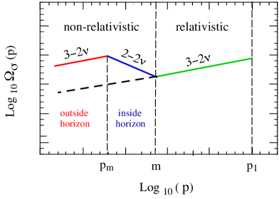
This conclusion, based on the effect illustrated in Fig. 7.3, refers however to a relativistic spectrum characterized by a constant slope. It is quite easy to imagine, however, and to implement in practice, a model of background in which the relativistic axion spectrum is sufficiently flat at low frequency (as required by a fit of the large-scale anisotropy), and much steeper at high frequency. A simple example is illustrated in Fig. 7.4, where we have compared two spectra. The top one is flat everywhere, except for modes becoming non-relativistic outside the horizon. The other one has a relativistic branch, which is flat at low frequency , and steeper at high frequency . It is evident that the steeper and the longer the high-frequency branch of the spectrum, the larger is the suppression of the amplitude at low frequency, and the larger is the axion mass allowed by the COBE normalization at the present Hubble scale .

This possibility has been analysed through an explicit two-parameter model of background [325], based on exact solutions of the low-energy string-cosmology equations with classical string sources [322, 303, 304]. By fixing the high-frequency normalization at , the low-frequency slope at , and the temperature of mass generation at MeV, we can use as parameters the slope and the duration of the high-frequency part of the spectrum, measured in particular by and by the corresponding variation of the pump field, . By imposing the COBE normalization (7.59), , the seed condition , and the condition of mass-dominated spectrum, (see [325]), the allowed region in parameter space turns out to be consistent with a very wide range of axion masses, from the equilibrium scale eV up to MeV (higher masses are not acceptable, because the axion would decay into photons before the present epoch, like dilatons, see Eq. (6.33)). We may thus conclude that there is no fundamental incompatibility between the normalization imposed by the large-scale anisotropy and an axion mass in the expected range of conventional axion models [567]. The difficulties encountered to match the observed spectrum at smaller angular scales, discussed in the previous subsection, remains however .
7.5 Massive axions and adiabatic perturbations
In the previous subsections we have analysed a possible scenario in which no axion background is present in the post-big bang epoch (), and an isocurvature, non-Gaussian spectrum of temperature anisotropies is eventually induced by the quantum fluctuations of the (massless or massive) axion field, amplified by inflation. This scenario, whose typical signatures have been discussed in Subsection 7.3, seems to be strongly disfavoured with respect to more conventional explanations of the CMB anisotropy offered by the standard inflationary models.
In this subsection we will consider a possible alternative picture, based on the following assumptions: i) the constant value of the axion background after the pre-big bang phase is displaced from the minimum (conventionally defined as ) of the non-perturbative potential generated in the post-big bang epoch; ii) the axion potential is strong enough to induce a phase of axion dominance before its decay into radiation. Under these conditions one finds that the initial isocurvature axion fluctuations, amplified by horizon-exit during inflation, can be converted into adiabatic (and Gaussian) perturbations of the spatial curvature, associated to super-horizon (scalar) metric perturbations, which maintain the same spectrum as the original axion fluctuations until the time of horizon re-entry: these can then possibly produce the observed CMB anisotropies.
This possibility, based on a mechanism originally pointed out in [487], has recently been discussed in detail (and not exclusively within a string cosmology framework) in [242, 460, 488, 66, 503, 489] for the isocurvature fluctuations of a generic scalar field (called “curvaton” [460]), amplified with a flat spectrum. In the context of the pre-big bang scenario, such a mechanism has been applied, in particular, to the fluctuations of the KR axion [242], as suggested in [438]. Here, after a brief description of the conversion of axion fluctuations into scalar curvature perturbations, we shall discuss the constraints imposed by the CMB data, and its possible consistency with the small-scale normalization and tilts typical of pre-big bang models [101].
The conversion of the axionic isocurvature modes into adiabatic curvature inhomogeneities takes place in the post-big-bang phase, where we assume the dilaton to be frozen and the axion to be displaced from the minimum of its potential. In the E-frame the background evolution is then described by the Einstein equations (6.2), with simply replaced by , and with since the axion is minimally coupled to the metric. For a conformally flat metric, , the time and space components of such equations, together with the axion evolution equation, can be written (in conformal time and in ) respectively as
| (7.85) | |||
| (7.86) |
where , is the energy density of the radiation fluid, and
| (7.87) |
The combination of Eqs. (7.85) and (7.86) leads to the conservation equation for the radiation fluid, i.e. . In order to perform analytical estimates, we shall also assume here that the axion potential can be approximated by the quadratic form . This is certainly true for , but it may be expected to be a realistic approximation also for the range of values of not much larger than (which, as we shall see, is the appropriate range for a normalization of the spectrum compatible with present data). Actually, for the periodic potential expected for an axion, the value of is effectively bounded from above [242].
Let us now consider the scalar perturbations of the Einstein equations (6.2). Working in the longitudinal gauge we set , and we use the perturbation variables already defined in Eq. (6.1) for the metric and for the fluid sources. We impose, in addition, (adiabatic fluid perturbations), and we introduce the convenient velocity potential , such that .
The perturbation of the component of the Einstein equations then gives , where is the Bardeen potential, while the perturbation of the (), (), () components, and of the axion (Klein–Gordon) equation, gives a set of four independent equations for the four scalar variables . They can be written, respectively, in the following convenient form:
| (7.88) | |||
| (7.89) | |||
| (7.90) | |||
| (7.91) |
where we have defined
| (7.92) |
The above equations can also be obtained directly from the general system of scalar-perturbation equations (6.3)–(6.8) (used to discuss dilaton production), for the particular case in which , , and with replaced by . We note, for later use, that by eliminating from Eqs. (7.89) and (7.90) we are led to
| (7.93) |
which, together with Eq. (7.91), provides a closed set of coupled differential equations for the two variables and . By using the above perturbation equations, together with the background relations (7.85) and (7.86), two useful equations for the evolution of and can be finally obtained:
| (7.94) |
We now suppose that we start at , with a radiation-dominated configuration in which the axion background is initially constant and non-vanishing, , , providing a subdominant (potential) energy density, . We also give initial conditions to our system of perturbation equations by assuming a given spectrum of isocurvature axion fluctuations, , and a total absence of perturbations for the metric and the radiation fluid, . The initial values of the first derivatives of the perturbation variables are then dedermined by the momentum and Hamiltonian constraints (7.88), (7.89).
In order to discuss the possible generation of curvature fluctuations we must now specify the details of the background evolution, taking into account that the axion, initially constant and subdominant, starts oscillating at a curvature scale (see Eq. (7.86)), and eventually decays (with gravitational strength) in radiation, at a scale . During the oscillating phase the kinetic and potential energy densities are equal on an average, so that and behaves like dust matter. Since , the radiation energy is always diluted faster, and the axion background tends to become dominant at a scale .
For an efficient conversion of the initial and fluctuations into and fluctuations it is further required [242, 460, 488] that the decay occurs after the beginning of the axion-dominated phase, i.e. . Depending upon the relative values of and (i.e. depending upon the value of , in Planck units) we have thus different options which will now be discussed separately.
If , and then , the axion starts oscillating (at a scale ) when the Universe is still radiation-dominated. During the oscillations the averaged potential energy density decreases like , i.e. the typical amplitude of the axion background decreases like , from its initial value down to the value at which . During this period (as the background is radiation-dominated), so that , and . Finally, the background remains axion-dominated until the decay scale . This model of background is thus consistent for , namely for
| (7.95) |
which leaves a wide allowed range for , if we recall the cosmological bounds on the mass following from the decay of a gravitationally coupled scalar [239, 241] (typically, TeV to avoid disturbing standard nucleosynthesis).
For this class of backgrounds we can now solve the coupled equations (7.91), (7.93), neglecting the terms in the (Fourier transformed) perturbation equations, since we are interested in modes well outside the horizon. We find (in cosmic time) that the Bardeen potential grows like during the initial radiation phase in which the axion is slow rolling, and like during the period of (radiation-dominated) axion oscillations:
| (7.96) | |||||
| (7.97) |
( and are dimensionless numbers of order o), where and . In the subsequent axion-dominated phase, preceeding the decay, the Bardeen potential finally oscillates around the value , with a resulting overall generation of curvature perturbations from to
| (7.98) |
where refers to averages over one oscillation period.
If , and then , the beginning of the oscillating and axion-dominated phase are nearly simultaneous, and the Bardeen potential only grows during the initial radiation-dominated phase, according to eq. (7.96). The final averaged value of the induced perturbations is now
| (7.99) |
Finally, if , and then , the axion starts dominating at the scale , which marks the beginning of a phase of slow-roll inflation, lasting until the curvature drops below the oscillation scale . Such a model of background is consistent for , namely for
| (7.100) |
where (fixed around the string scale) corresponds to the beginning of the radiation-dominated, post-big bang evolution. During the inflationary phase the slow decrease of the Hubble scale can be approssimated (according to the background equations (7.85) and (7.86)) as , where and are dimensionless coefficients of order . Inflation thus begins at the epoch , and lasts until the epoch . Let us estimate, for this background, the evolution of the Bardeen potential generated by the primordial axion fluctuations.
For the solution is still given by eq. (7.96), with replaced by . At the beginning of inflation the averaged amplitude is then . During slow-roll inflation, on the other hand, it is known [493] that, for superhorizon modes, . The final amplitude at the beginning of the oscillating phase is then
| (7.101) |
and no further amplification is expected in the course of the subsequent cosmological evolution.
It is amusing to observe that the results (7.98), (7.99), (7.101), which determine the amplitude of the Bardeen potential in the oscillating (axion-dominated) phase preceding the axion decay, can be summarized by an equation that holds in all cases, namely
| (7.102) |
where are numerical coefficients of the order of unity. A preliminary fit [101] based on numerical and analytical integrations of the perturbation equations gives . The function has the interesting feature that it is approximately invariant under the transformation and, as a consequence, has a minimal value around .
Given , we can easily compute the final value (before axion decay) of the density constrasts , and of the variable parametrizing in a gauge-invariant way the strength of curvature perturbations. By using the background equations (7.85) in the axion-dominated phase, , and taking the average of Eq. (7.89), for super-horizon modes, one finds indeed (averaging being understood) . Similarly, from Eqs. (7.94), and for super-horizon modes, .
Consider then the variable representing the perturbation of the spatial curvature on uniform density hypersurfaces, which is conserved (outside the horizon) for adiabatic perturbations, and which can be written for a general background as [493]:
| (7.103) |
Outside the horizon we can use for , the sum of the two background equations (7.85) for the denominator , and the Hamiltonian constraint (7.89) for the numerator , in order to rewrite in the form
| (7.104) |
In the final phase dominated by an oscillating axion is negligible, the (averaged) axion pressure is zero so that, using we finally obtain
| (7.105) |
(as we have also checked by an explicit numerical integration [101]). This result was derived and presented in [460], using however different notations.
The generated spectrum of super-horizon curvature perturbations is thus directly determined by the primordial spectrum of isocurvature axion fluctuations , according to Eqs. (7.102) and (7.105). The axion fluctuations, on the other hand, are solutions (with pre-big bang initial conditions) of the perturbation equation (7.91) in the radiation era (no additional amplification is expected, for super-horizon modes, in the axion-dominated phase), computed for negligible curvature perturbations () in the massive, non-relativistic limit (as we are already in the oscillating regime), and outside the horizon.
In order to exploit the results of the previous subsection, we can then set , where satisfies Eq. (7.69). The general solution for , correctly normalized to a relativistic spectrum of quantum fluctuations, has been given in Eq. (7.78) already, taking also into account the details of the pre-big bang amplification (encoded into the Bogoliubov coefficient ). Outside the horizon, , and for non-relativistic modes, , we take (respectively) the limits and , in which . By inserting a generic, primordial power-law spectrum with cut-off scale , i.e. , and using the identity , we finally obtain the generated spectrum of curvature perturbations:
| (7.106) |
We have re-inserted the appropriate Planck mass factors, keeping however dimensionless in Planck units, and we have included into possible numerical factors of order , connecting the cut-off scale to the string mass scale
This result, valid during the axion-dominated phase, has to be transferred to the phase of standard evolution, by matching the (well known [493]) solution of the Bardeen potential in the radiation era (subsequent to axion decay) to the solution prior to decay, which is in general oscillating. The matching of and , conventionally performed at the fixed scale , shows that the constant asymptotic value (7.102) of super-horizon modes is preserved to leading order by the decay process, modulo a random, mass-dependent correction which typically takes the form , where is a numerical coefficient of order , and . Such a random factor, however, is a consequence of the sudden approximation adopted to describe the decay process, and disappears in a more realistic treatment in which the evolution equations for and are supplemented by the friction term (with a corresponding antifriction term in the radiation equation).
In such a way, as we have checked with an numerical integration, the decay process preserves the value of the Bardeen potential prior to decay, damping the residual oscillations; itself follows the same behaviour and is finally exactly a constant. When the axion has completely decayed, and the Universe is again dominated by radiation, we can properly match the standard evolution of in the radiation phase to the constant asymptotic value of Eq. (7.102). The expression we obtain for the Bardeen potential, valid until the epoch of matter–radiation equality, can be written in the form
| (7.107) |
where and is given in Eq. (7.102).
The above expression for the Bardeen potential provides the initial condition for the evolution of the CMB-temperature fluctuations, and the formation of their oscillatory pattern. It is important to note that, from the above equation, and , where , and . This implies [101] that the induced temperature fluctuations will oscillate in just as expected in the case of adiabatic perturbations, producing a peak structure clearly distinguishable (and, at present, observationally favoured) from that produced by isocurvature fluctuations.
Let us now discuss the large scale normalization of the induced anisotropies, starting from the observation that the final amplitude of the super-horizon perturbations (7.106) seems to be unaffected by the non-relativistic corrections to the axion spectrum. The dependence on the axion mass appears, however, when computing the amplitude of the spectrum at the present horizon scale , in order to impose the corrected normalization to the quadrupole coefficient , namely [223]
| (7.108) |
where the value of is experimentally determined by COBE according to Eq. (7.53).
The present value of the cut-off frequency, , depends in fact on the kinematics as well as on the duration of the axion-dominated phase (and thus on the axion mass), as follows:
| (7.109) | |||||
| (7.110) |
Using , we find that the COBE normalization imposes
| (7.111) | |||
| (7.112) |
where denotes the amplification of the scale factor during the phase of axion-dominated, slow-roll inflation.
The condition (7.111) is to be combined with the constraint (7.95), the condition (7.112) with the constraint (7.100), which are required for the consistency of the corresponding classes of background evolution. Also, both conditions are to be intersected with the experimentally allowed range of the spectral index. The allowed range of parameters compatible with all the constraints is rather strongly sensitive to the values of the pre-big bang inflation scale . In the context of minimal models of pre-big bang inflation we have , and a flat spectrum () is inconsistent with the normalization (7.111), (7.112). A growing (“blue”) spectrum is instead allowed (see [101] for a detailed discussion). It turns out, in particular, that there is a wide range of allowed axion masses, but a rather narrow range of allowed values for , especially in the case .
The allowed range of parameters is extended if the inflation scale is lowered, and a flat () spectrum may become possible if , for , and if , for (see Eqs. (7.111) and (7.112)). A lower value of the string scale could emerge indeed in a recently proposed framework [608] according to which, at strong bare-coupling , loop effects renormalize downwards the ratio and allow to approach the unification scale.
In addition, a flat spectrum may be allowed even keeping pre-big bang inflation at a high-curvature scale, provided the relativistic branch of the primordial axion fluctuations is characterized by a frequency-dependent slope, which is flat enough at low frequency (to agree with large-scale observations) and much steeper at high frequencies (to match the string normalization at the end-point of the spectrum). A typical example of such a spectrum, already introduced in the previous subsection, and illustrated in Fig. 7.4, can be parametrized by a Bogoliubov coefficient with a break at the intermediate scale ,
| (7.113) | |||||
where parametrizes the slope of the break at high frequency. Examples of realistic pre-big bang backgrounds producing such a spectrum of axion fluctuations have been discussed in [325]. It is clear that the steeper (and the longer) the high-frequency branch of the spectrum, the easier the matching of the amplitude to the measured anisotropies (in spite of possible -dependent enhancements).
Using the generalized input (7.113) for the spectrum of , the amplitude of the low-frequency () Bardeen spectrum (7.106) is to be multiplied by the suppression factor , and the normalization condition at the COBE scale becomes
| (7.114) | |||
| (7.115) |
A strictly flat spectrum is now possible, even for , provided
| (7.116) |
It thus becomes possible, in this context, to satisfy the stringent limits imposed by the most recent analyses of the peak and dip structure of the spectrum at small scales [205], which imply .
We may thus conclude that, in the context of the pre-big bang scenario, a “curvaton” model based on the Kalb–Ramond axion is able to produce the adiabatic curvature perturbation needed to explain the observed large-scale anisotropies. The simplest, minimal models of pre-big bang inflation seem to prefer blue spectra. A strictly scale-invariant (or even slightly red, ) spectrum is not excluded but requires, for normalization purposes, non-minimal models of pre-big bang evolution leading to axion fluctuations with a sufficiently steep slope at high frequencies.
8 Singularity and “graceful exit”
As already stressed in Section 2, the cosmological solutions of the string effective action, thanks to their symmetries, are characterized by four branches, which are inter-related by time-reversal and scale-factor duality transformations. Two branches are of the pre-big bang type, and evolve towards a singularity, while the other two branches are of the post-big bang type, and emerge from a singularity. A typical example is illustrated in Fig. 8.1, where we have plotted the asymptotic, -dimensional vacuum solutions of the lowest-order gravidilaton effective action,
| (8.1) |
which represent the bisecting lines of the “phase space” spanned by the variables . The initial conditions of the pre-big bang scenario and the present standard cosmological configuration are thus disconnected by a singularity localized at the future or past end, respectively, of the temporal half-line on which they are defined.
In the case of homogeneous and isotropic metric backgrounds, with or without spatial curvature, there are “no-go theorems” [127, 396, 397, 234] that exclude the possibility of a smooth transition from the pre- to the post-big bang branch of the tree-level solutions, even including a (local) dilaton potential , and matter sources in the form of perfect fluids and/or an homogeneous NS-NS two-form. In all these cases the singularity cannot be removed. In addition, in the absence of sources and of a dilaton potential, it is known that the singularity also affects anisotropic backgrounds, and can be shown to be generally present in all homogeneous four-dimensional metrics of Bianchi type I, II, III, V, and [313].
We are thus led to the problem of explaining how the Universe may smoothly evolve from the string perturbative vacuum, and from an initial accelerated growth of the curvature and of the string coupling, to a final, decelerated, post-big bang configuration, which is certainly included in the set of string-cosmology solutions, but is possibly disconnected from the initial pre-big bang branch by a curvature singularity. This is the so-called “graceful exit” problem.
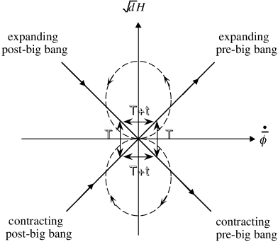
The exit from inflation, and a smooth description of the transition from accelerated to decelerated expansion, is a typical problem of all inflationary models (see for instance [56]). In the string cosmology case, however, such a problem is sharpened by the fact that the transition from the pre- to the post-big bang phase is expected to occur at high curvature and strong coupling, possibly in the full quantum-gravity regime. This may suggest that a correct approach to the exit problem is to be developed in a quantum cosmology context, by exploiting the Wheeler-De Witt equation in the string cosmology minisuperspace, and the associated symmetry, which helps avoiding operator ordering ambiguities [311, 411].
In this approach, interesting in itself, the probability of quantum transition from the pre- to the post-big bang branches of the low-energy solutions can be finite and non-vanishing, even if the two branches are classically disconnected by a singularity [311, 323]. This possibility will be presented in detail in Section 9. In this section we shall keep on a classical (i.e. deterministic) description of the exit, which requires the smoothing out of the background singularities.
It should be stressed, in particular, that the phenomenological predictions made in the previous sections were based on the assumption that the singularity can be regularized, and that i) a graceful exit does take place; ii) sufficiently large scales are only affected by it kinematically, i.e. through an overall redshift of all scales. Of course, one would not only like to know that a graceful exit does take place: one would also like to describe the transition between the two phases in a quantitative way. Achieving this goal would amount to nothing less than a full description of what replaces the big bang of standard cosmology in the pre-big bang scenario. As mentioned in Section 1, this problem of string cosmology is the analogue, in some sense, of the (still not fully solved) confinement problem of QCD.
The problem of the background regularization is particularly hard because, besides the smoothing out of the curvature, it also requires the smoothing out of the dilaton kinetic energy, and a possible damping of the dilaton (i.e. of the string coupling). We may consider, for a simple illustrative example of this point, the lowest-order gravidilaton action, supplemented by a matter action that describes perfect-fluid sources, with vanishing dilatonic charge, :
| (8.2) |
By assuming an isotropic, spatially flat metric background, with spatial sections of finite volume, we set
| (8.3) |
For , , the field equations can be written in the form
| (8.4) | |||
| (8.5) | |||
| (8.6) |
where , (see Subsection 2.2), and we have used units in which . Their combination gives the conservation equation
| (8.7) |
The above equations can be satisfied by the following particular exact solution
| (8.8) |
where is an arbitrary integration constant. The integration of then leads to the implicit expression for the scale factor,
| (8.9) |
This solution is self-dual, in the sense that , , , and describes a smooth evolution of the metric from an initial, accelerated phase of growing curvature and negative pressure, to a final, decelerated phase of decreasing curvature and positive pressure. The scale factor runs monotonically from zero to infinity, without any curvature singularity.
This example cannot be accepted as a successful model of exit, however, because the dilaton kinetic energy () blows up at the transition point (), together with the effective string coupling, . This implies that both and loop corrections to the effective action become non-negligible at the transition, and that the above solution, obtained in the low-energy, tree-level approximation, cannot be trusted. In addition, the curvature is regular in the string frame, but blows up in the Einstein frame defined by
| (8.10) |
(see for instance Subsection 1.3). Indeed, by setting and , we obtain
| (8.11) |
so that, if the dilaton is unbounded, may diverge even if both and are regular.
A successful exit thus requires a smooth dilaton evolution, with the kinetic energy and bounded everywhere. In addition, the dilaton has to evolve from the initial regime with to a final regime with (see Fig. 8.1); besides being bounded, at large positive times, its kinetic energy must thus satisfy the condition
| (8.12) |
This is not sufficient, however, for a complete exit. An even stronger condition is imposed by requiring that the final, post-big bang configuration may describe (even in the E-frame) a phase of decelerated expansion, after the contraction representing pre-big bang inflation (after all, the String and Einstein frames are doomed to coincide, eventually, in the limit of dilaton stabilization). This implies at large positive times or, according to Eq. (8.11),
| (8.13) |
The above constraints can be translated into energy conditions, to be satisfied by the stress tensor of the effective sources driving the exit transition [122, 123].
In spite of such constraints, there are simple examples of regular backgrounds implementing a successful exit by means of appropriate sources, as we shall see in Subsection 8.1. The simplest examples, however, are not very realistic. The most realistic physical mechanism of exit, in the perturbative regime, is probably based on the backreaction of the quantum fluctuations, which leads, however, to including loops (and possibly higher derivative) corrections in the effective action, as we shall discuss in Subsections 8.2 and 8.3. Such corrections suggest possible lines along which a quantitative description of the exit might eventually emerge.
The loop corrections, however, become important in the strong coupling regime, i.e. in the realm of the still largely unknown M-theory [627, 377], as will be discussed in Subsection 8.5. It is thus possible that, in spite of the existing encouraging results, new techniques and/or a deeper understanding of string theory in its non-perturbative regimes need be developed (see [111] for a recent attempt), before a fully satisfactory description of the transition from pre- to post-big bang can be hoped for.
In the next subsection we will start presenting a few simple examples of smooth solutions, without curvature singularities, obtained in the context of the low-energy string effective action.
8.1 Smoothing out the singularity at low energy
It is well known, from the singularity theorems of general relativity (see for instance [373, 372, 616]), that a smooth and complete geometrical background, with all the curvature invariants bounded everywhere, is only allowed if the sources of the gravitational field satisfy appropriate energy conditions.
In the context of the string cosmology equations, the situation is even more constrained, because also the string coupling , parametrized by the dilaton, has to be bounded (and possibly smaller than ) for a consistent and appropriate use of the string effective action (and of the perturbative expansion). In addition, if the curvature and the dilaton kinetic energy are regular in the S-frame, but the dilaton is free to grow boundlessly, then divergences may appear in the E-frame according to Eq. (8.11). This may occur, for instance, if the regularization of the curvature in the S-frame leads to a phase of constant and , as in the context of the higher-order effective action [295, 308], which will be discussed in Subsection 8.3. The importance of a frame-independent regularization is stressed by the fact that some particles, such as the gravitons, follow the E-frame geodesics [400].
In spite of such difficulties, examples of smooth, self-dual solutions with no curvature singularities have been obtained, even in the context of the lowest-order string effective action, and of homogeneous and isotropic backgrounds, by introducing however ad hoc a negative and non-local dilaton potential [478, 320, 311], . Such a potential, which only makes sense for manifolds with spatial sections of finite volume, (for instance, a torus), is non-local because , to be a generally covariant scalar, must contain the integral of the whole spatial volume (see Subsection 1.4).
Consider, as an example, the action (8.2), with a dilaton potential . The field equations, for an isotropic and spatially flat metric, become ()
| (8.14) | |||
| (8.15) | |||
| (8.16) |
and the conservation equation (8.7) is still valid. In the vacuum case , the full set of equations can be integrated exactly [478], and one finds that non-singular solutions are in general allowed. If we consider, for instance, the potential [311]
| (8.17) |
the above equations can be exactly satisfied by the particular solution
| (8.18) |
where and are integration constants.
This is a regular self-dual solution, , characterized by a bounded, “bell-like” shape not only of but also of the dilaton kinetic energy (unlike the example given in Eq. (8.8)). For the solution satisfies the conditions (8.12), (8.13) required for a successful exit [122, 123] and, together with its time-reversed partner, it describes indeed a perfect “-shaped” curve in the plane of Fig. 8.1. Such a solution smoothly interpolates between the asymptotic branches (8.1) of the vacuum solutions, i.e. from the superinflationary expansion , at , to the final state of decelerated expansion and decreasing curvature , at (see Figs. 8.2 and 8.3).
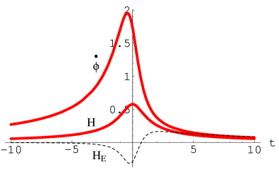
It is important to note that in this solution the dilaton is monotonically growing (indeed, for , ), but the curvature is regular even in the E-frame, where smoothly evolves from the pre-big bang accelerated contraction at , to a phase of decelerated expansion at . For , in fact, , so that the E-frame curvature is bounded for all . The fact that the dilaton keeps growing, however, is not consistent (asymptotically) with the perturbative approach, and with the use of the lowest-order string effective action. In addition, the curvature may blow up in some other frame, different from the String and Einstein ones.
A more satisfactory example of transition, in which the dilaton becomes asymptotically frozen in the radiation-dominated regime, can be implemented by using another form of non-local dilaton potential [320],
| (8.19) |
In that case Eqs. (8.14)–(8.16) can be integrated exactly, for a wide class of (possibly time-dependent) equations of state. Let us report in some detail the integration procedure already outlined in Subsection 2.3, which is also useful for further applications.
We start by defining a new (dimensionless) time coordinate , such that
| (8.20) |
( is a constant parameter with dimensions of a length). The combination of Eqs. (8.14), (8.16), using the relation , gives
| (8.21) |
where a prime denotes the differentiation with respect to , and is an integration constant. By assuming a time-dependent equation of state, defined by the function such that
| (8.22) |
Eq. (8.15) can be rewritten as
| (8.23) |
The matter-conservation equation (8.7), on the other hand, gives
| (8.24) |
By summing Eqs. (8.21), (8.24), and integrating, we are led to defininig the function such that
| (8.25) |
( is an integration constant), and our system of equations for and can be reduced to quadratures:
| (8.26) |
We have to satisfy, finally, Eq. (8.14), which determines the constant through the condition
| (8.27) |
There are two possibilities. The first one is trivial: and . The second solution, valid for the potential (8.19), is
| (8.28) |
In such a case the integration of Eqs. (8.26) may provide regular solutions, with bounded curvature, kinetic terms and dilaton, describing a smooth evolution from the pre- to the post-big bang regime [320].
The simplest examples of regular solutions are obtained in the case of perfect fluids, with equation of state const. From Eq. (8.22) one finds indeed , where is an integration constant and, if , it is always possible to choose in such a way that has no zeros, and the solution is regular. See [320], in particular, for the radiation case with . But, in general, we may also describe a smooth evolution, which ends up with radiation, starting from its dual equation of state, , corresponding to a gas of stretched strings (typical example of a pre-big bang phase dominated by string sources, see Section 2). If we take, for instance [320],
| (8.29) |
and we choose , the integration of Eqs. (8.26) gives in fact
| (8.30) | |||
| (8.31) |
This solution is self-dual, , and describes a model that is always exapnding, . The Universe, starting at from the flat space () and weak coupling () regime, evolves through a superinflationary phase () dominated by unstable string matter (), towards the standard radiation-dominated phase (, ), with frozen dilaton ( const). The curvature parameters , and the coupling , are everywhere bounded (see Fig. 8.3).
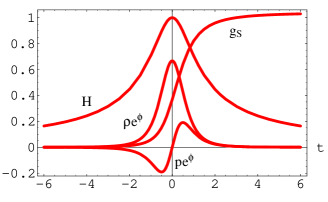
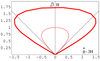
It should be noted that with different, more general choices of and , the solution contains, in general, an intermediate stage of contraction before the final radiation phase [30], but even in that case the curvature and the dilaton keep bounded. The above solution can also be generalized to anisotropic configurations, describing graceful exit from inflation and, simultaneously, dynamical dimensional reduction [320]. In that case, besides the expanding dimensions, there are also shrinking internal dimensions that evolve from accelerated contraction (driven by an internal positive pressure) to a final decelerated contraction (driven by negative pressure).
Without non-local potential and matter sources, smooth solutions can be obtained by relaxing the isotropy and/or homogeneity assumptions. There are indeed particular examples, in the context of the lowest-order string effective action, in which the curvature singularities can be regularized by performing an appropriate transformation, which introduces, however, a non-trivial anisotropic axion background (it is tempting to speculate that this softening of singularities, due to a non-trivial field, could be related to recent developments in the field of non-commutative geometry [220], also induced by a field).
The simplest example [309] is the boost of the trivially flat, Milne-type exact solution of the gravidilaton action (8.2) (with );
| (8.32) |
or of its (singular) scale-factor duality partner:
| (8.33) |
( are “inert” coordinates spanning a -dimensional Euclidean space). Consider in fact the transformation, in the plane, generated by the one-parameter matrix such that
| (8.34) |
(here and are the , part of the metric and of the antisymmetric tensor). We obtain a new class of exact solutions of the string effective action, with non-trivial , represented by [309]
| (8.35) |
where the upper and lower signs refer, respectively, to the boost of the solution (8.32) and (8.33).
For such solutions, all the curvature invariants are bounded [309], as well as the dilaton coupling , so that the solutions are regular in all frames. They describe a smooth evolution from (anisotropic) contraction to expansion, or vice versa, according to the behaviour of the original metric (the Milne-type solution or its dual). In any case, the boosted backgrounds (8.35) evolve from growing to decreasing curvature, and from growing to decreasing dilaton, as appropriate to a transition from pre- to post-big bang configurations. The new solutions are highly anisotropic, but the associated shear tensor rapidly decays far from the high-curvature regime [309]. Taking into account the backreaction of the produced radiation it is also possible to obtain a more realistic scenario, in which the background is eventually led to a phase of radiation-dominated, isotropic expansion, at constant dilaton [285].
More complicated, inhomogeneous examples of (non-trivial) regular backgrounds at low energy are provided by the “boosted” version of the Nappi–Witten solution [498]. We start with the following (singular) exact solution of the action (8.2) with ,
| (8.36) |
representing the direct product of a two-dimensional cosmological metric in the plane and a two-dimensional Euclidean black hole in the plane. Since the metric is independent of and we can apply to it any transformation in the plane, to obtain new classes of inequivalent solutions. In particular, the transformation generated by the matrix
| (8.37) |
generates the one-parameter family of inhomogeneous (and singular) Nappi–Witten cosmologies [498].
As in the previous example, the singularities of the solution (8.36) can be removed by introducing an additional (originally flat) spatial dimension, parametrized by the coordinate . The model then acquires a larger symmetry, isomorphic to , in the subspace . Performing two successive “boost” transformations (with the same parameter as in Eq. (8.34)) in the plane and in the plane, one can obtain a new class of inhomogeneous exact solutions completely free from curvature and dilaton singularities (see [310] for an explicit computation). As an example we report here the curvature scalar and the coupling of the boosted solutions [310]:
| (8.38) |
The curvature and the dilaton are bounded, but the background is too inhomogeneous to provide a realistic description of our present Universe. Such solutions could be relevant, however, to descrive the Universe near the transition regime, before the beginning of the standard radiation era.
The same comment applies to another class of regular inhomogeneous solutions of the lowest-order action (8.2), which is obtained even in the absence of torsion () and dilaton potential, and which can be parametrized in diagonal form as [331]
| (8.39) |
where:
| (8.40) |
Here , and are constant parameters, and is the so-called “Gudermannian amplitude”. As shown in [331, 333], there are particular values of for which the curvature invariants are bounded, the solutions are geodesically complete and describe a phase of growing dilaton coupling, evolving from a minimum up to a maximal value. We note that there is also another family of inhomogeneous solutions of the gravidilaton equations in which all curvature invariants are bounded [520], which is parametrized by a non-diagonal metric and reduces, in the E-frame, to known regular solutions of the Einstein equations with stiff sources [473]. In that case, however, the dilaton grows linearly and boundlessly.
We may thus conclude that, as in general relativity [563, 473], if the metric background is allowed to be inhomogeneous there is no need of a non-local potential and/or antisymmetric tensor densities to obtain regular cosmological solutions, even in the contex of the lowest order gravidilaton action.
To stress the difficulty in obtaining smooth solutions in the homogeneous and isotropic case, on the contrary, we will conclude this subsection with a simple example, based on a Bianchi-I-type metric, and barotropic (but anisotropic) fluid sources with constant dilaton charge per unit mass:
| (8.41) |
where is the matter action of Eq. (8.2), and are constant parameters specifying the “equation of state” of the fluid sources. The corresponding cosmological equations can be written in the form
| (8.42) | |||
| (8.43) | |||
| (8.44) |
Following the procedure already applied to the case of the non-local potential (8.19), the above equations can be integrated exactly in terms of the time coordinate (8.20), and we obtain [212]
| (8.45) | |||
| (8.46) |
where
| (8.47) |
and are integration constants. In the case and/or , a slightly different definition of the quadratic form is obtained, as well as a different expression for and , but in that case no smooth solution with bounded curvature and energy density is allowed, for any value of . We will thus concentrate on Eqs. (8.45)–(8.47) (see [212] for a discussion of the other possibilities).
By setting it can easily be checked that if the background is isotropic (i.e. and have the same values along all the spatial directions), then the discriminant of is always non-negative, i.e. , so that necessarily has zeros on the real axis, correponding to singularities both in the curvature and in the dilaton kinetic energy. Such singularities can be avoided, however, for anisotropic backgrounds, provided we accept a model of sources with negative energy density, .
Consider for instance a model of background in which the spatial geometry is factorizable as the direct product of two conformally flat manifolds with and dimensions, respectively, so that we can set:
| (8.48) |
and choose a convenient set of integration constants, such that the linear term in the quadratic form (8.47) disappears. For instance:
| (8.49) |
It turns out that , and that the absence of zeros in can be avoided, , provided
| (8.50) |
With the above assumptions, the integration of Eqs. (8.45), (8.46) leads to the final solution
| (8.51) |
where are integration constants. As shown in [212], there is a region of non-zero extension in the space of the parameters where the condition (8.50) is satisfied, together with the other conditions needed to secure that the curvature, the dilaton kinetic energy, the effective string coupling, the energy density are everywhere bounded, that the density goes asymptotically to zero at large times, and that the solution describes in its final configuration expanding and contracting dimensions (as appropriate to a smooth transition from a higher-dimensional pre-big bang configuration to a post-big bang regime of dynamical dimensional reduction).
The condition (8.50) implies, however, that everywhere, and thus , according to Eq. (8.47) (the result in the absence of zeros is independent from the particular choice ). Such a result is not surprising, after all, because also the regular solutions obtained in the case of negative non-local potentials correspond to a negative energy density. See also [236] for another class of smooth, self-dual solutions of the low-energy effective action in which the energy density of the matter sources becomes negative, near the transition, because of an “exotic” equation of state.
In the above example the negative energy density goes to zero, asymptotically, far from the transition regime, and can thus be interpreted as the backreaction of the quantum fluctuations outside the horizon [212]. During the initial pre-big bang phase of growing curvature and shrinking horizons, in fact, the quantum fluctuations are stretched outside the horizon, and in such regime they may be characterized by a negative effective gravitational energy density [495, 496], which may favour the transition to the post-big bang branch of the classical solution [345]. Such a negative backreaction is eventually damped to zero when the curvature starts decreasing, the horizon blows up again, and all the fluctuations re-enter inside the horizon and in the regime of positive energy density.
The inclusion of the backreaction of the quantum fluctuation, on the other hand, is also a semiclassical way of taking into account the contribution of the quantum loop corrections to the effective action. Thus, the examples of graceful exit reported in this subsection, based on effective sources (fluid or non-local potential) with , which become dominant just around the epoch of transition, suggest the possible importance of the quantum backreaction –and of the loop corrections to the string effective action– for a successful mechanism of curvature and dilaton regularization. This possibility will be illustrated in Subsection 8.3, after a preliminary discussion of the effects of the higher-curvature corrections, which will be presented in the next subsection.
8.2 Growth of the curvature and corrections
The effective action of string theory is characterized by two perturbative expansions: the higher-genus expansion in the world-sheet topology, and the order-by-order condition of vanishing conformal anomaly, also called expansion [347]. The first one is equivalent to the quantum, field-theoretical loop expansion in powers of the coupling; the second one is equivalent to a higher-curvature expansion in powers of the field gradients (in units of ). The second one is typical of strings, and disappears in the point-like limit .
These two expansions are indepedent in principle; it is possible, depending on the initial conditions, that the Universe evolving from the string perturbative vacuum reaches the strong-coupling regime when the curvature is still small, and the corrections are negligible. Alternatively, the Universe can reach the regime of high curvatures (in string units) when the coupling is small: in that case, only the corrections are to be added to the tree-level action.
What is important, in the context of the exit problem, is that such higher-curvature corrections may help the transition to the post-big bang regime, by damping the inflationary growth of the dilaton and of the curvature, and driving the cosmological background to a high-curvature “string phase” of constant curvature and linearly evolving dilaton [308], const, const.
Remarkably, such a regularized background can be a solution of the tree-level effective action to all orders in . Indeed, as shown in [308], for a Bianchi-I-type configuration with , , with constant and , the string cosmology equations reduce (to all orders in ) to a system of algebraic equations for the unknowns . String-phase solutions thus generally exist, provided the algebraic system admits (non-trivial) real solutions.
In addition, the (all orders) equations resemble those of a renormalization group flow (in cosmic time), with the string-phase solution like a “fixed point” of the renormalization equations. It can thus be shown [308] that a string phase solution with can play the role of late-time attractor for an isotropic Universe evolving from pre-big bang initial conditions, provided no other fixed point, or singularity, separates the string phase from the string perturbative vacuum (i.e. from the trivial fixed point with ).
A simple example of this possibility, first presented in [308], is based on the following S-frame effective action, truncated to first order in :
| (8.52) |
( is a number of order depending on the particular string model adopted). Note that we have chosen a convenient field redefinition (preserving the conformal invariance of the -model action [483]) that eliminates higher than second derivatives from the equations of motion, but at the price of introducing dilaton-dependent corrections.
For a spatially flat anisotropic background, with external and internal dimensions,
| (8.53) |
the action becomes
| (8.54) | |||||
where are dimensionless numerical coefficients depending on and (see [308]). By varying the action with respect to and , and setting , const, const (in the gauge ), we are led to the algebraic equations for an isotropic fixed point:
| (8.55) |
which have real solutions for any from to . For instance (in units )
| (8.56) |
where the same sign has to be taken for and . Note that, with the addition of a non-zero background, anisotropic fixed-point configurations can also be obtained, as shown in [258].
A numerical integration of the isotropic cosmological equations, starting from pre-big bang initial conditions (, ), shows that the background, when the corrections become important, deviates from the tracks of the low-energy, singular solutions, and is eventually attracted to the isotropic fixed point (8.55), as illustrated in Fig. 8.4. In this sense, the curvature singularity is regularized by the corrections, at least in the S-frame (but not in the E-frame, as the linear growth of the dilaton is unbounded). Note that a similar curvature regularization is also effective for a static, spherically symmetric solution of the action (8.52) [132]. It should be mentioned that a similar behaviour can also be obtained at low energy (without corrections), including the contribution of a supersymmetric gravitino–dilatino condensate, which is able to damp the acceleration of the background and to regularize the S-frame curvature, as shown in [259].
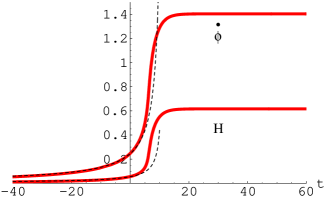
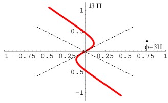
It may be noted, finally, that a solution with const, const is in general allowed in many higher-derivative models of gravity. Such a fixed point of the cosmological equations, however, is in general disconnected from the trivial fixed point (the perturbative vacuum, in this case) by a singularity, or by an unphysical region in which the curvature becomes imaginary. For the action (8.52), on the contrary, the constant fixed point is a late-time attractor for all isotropic backgrounds emerging from the string perturbative vacuum, and even for some anisotropic backgrounds, provided sign{}= sign{} (the attraction basin of anisotropic configurations covers regions of small but finite size in the space of initial conditions [308]).
This attraction property, unfortunately, is not invariant under field redefinitions, as long as the action is truncated at a given finite order in . Also, and most important, the growth of the curvature is stopped, but the transition is not completely performed. Indeed, the final fixed point is in the post-big bang regime , as illustrated in Fig. 8.4, but the transition cannot proceed further towards lower curvatures to complete the transition.
The reason for such an incompleteness, which is manifest as an asymmetry in the plane of Fig. 8.4, is that the action (8.52) is invariant under time reflections, but is not duality-invariant. As a consequence, the regularization concerns the expanding pre-big bang branch of the lowest-order solution, and its time-symmetric counterpart, the contracting post-big bang branch. The expanding post-big bang branch remains, however, singular, and thus cannot be smoothly connected to the regularized pre-big bang branch.
It is possible, of course, to modify the action with an additional field redefinition truncated to order , in such a way as to preserve conformal invariance and to restore the -duality symmetry (to the same order in ) [477, 398]. The modified action has then self-dual fixed points, but they are not smoothly connected to the perturbative vacuum, as we have checked. See also [124, 150] for a discussion of the existence and position of the fixed points in relation to the scale-factor duality of the higher-order action, and for the difficulty of a higher-order, self-dual model of exit.
The evolution of the background away from the fixed points, towards the low-energy, post-big bang regime, becomes however possible if the action (8.52) is further generalized by the inclusion of quantum loop correction (after all, the dilaton keeps growing while the Universe is trapped in the fixed point, so that higher-order effects in the string coupling are doomed to become eventually important). This point will be illustrated in the next subsection.
It should be noted, finally, that all examples of exit based on a truncated expansion are characterized by a certain degree of ambiguity, because the physical properties of such models are field-redefinition-dependent [308], as already stressed. A truly unambiguous example of exit should in principle correspond to the solution of an exact conformal model, which automatically includes all orders in (see [463], however, for a different non-perturbative approach to higher-order corrections, based on the inclusion of the exponentially growing density of all massive string-theory states, and on their possible role in regularizing the singularity).
There are in fact higher-curvature, exact conformal-field theory models that smoothly interpolate between two duality-related low-energy solutions [417, 418]. In that cases, however, it turns out impossible, in general, to describe the high-curvature regime in terms of classical fields such as the metric and the dilaton, and we may lose an intuitive and geometrical understanding of the transition (the conventional space-time interpretation is also lost in other, higher-dimensional, string-theory resolutions of the cosmological singularities [427]).
Exact conformal models, for and string-cosmology backgrounds, have been recently studied [216] in the context of gauged Wess–Zumino–Witten models [626], for the and cosets. It turns out that it is possible, in some cases, to avoid the curvature singularities, but the dilaton (and the string coupling) seems to remain unbounded in correspondence of inflationary backgrounds.
To conclude this subsection, devoted to higher-derivative corrections, we recall that a higher-curvature regularization of the cosmological singularity can also be obtained in the context of models implementing the so-called “limiting-curvature hypothesis” [492, 109, 486], applied to string cosmology in both the Einstein [105] and String [231] frames. They are based on a higher-derivative action which, in the S-frame, takes the form
| (8.57) |
where and are constant parameters, is a scalar Lagrangian multiplier, and
| (8.58) |
Finally, is a potential that satisfies appropriate boundary conditions, for , const for , and has non-trivial zeros.
Numerical and analytical studies then show that this action has regular spatially flat and isotropic solutions, smoothly interpolating from contraction to expansion in the E-frame [105], and from superinflation to decelerated expansion in the S-frame [231], even at constant dilaton. A dynamical dilaton may increase the fraction of phase space for which the curvature is bounded (in the absence of an appropriate potential, however, a dynamical dilaton keeps growing). Unfortunately (and as in other models that will be discussed in the next subsection), the action (8.57) is not derived from a string-theory expansion (the higher-order terms are artificially constructed), so that the obtained results are only valid as (interesting) phenomenological examples of possible approaches to the exit transition.
8.3 Growth of the coupling and loop corrections
According to the pre-big bang scenario, the tree-level effective action (8.2) can provide a correct description of the Universe at low energies, during the initial evolution leading the Universe away from the string perturbative vacuum, until the string coupling remains small, . However, since is growing during pre-big bang inflation, in the absence of a mechanism able to stop the growth of the dilaton, the Universe will tend to evolve towards strong couplings, . In that regime all the higher-loop contributions will become important, and since the fully corrected action is unknown, in general, we have to restrict our studies to the simplest cases where we know the explicit form of the loop corrections.
In all cases so far analysed in the literature, it was found that the inclusion of appropriate higher-order terms seems to damp the growth of and , thus favouring the exit transition. Indeed, in the presence of loop corrections, the “theorems” on the impossibility of branch changing have to be generalized [548]; it becomes possible, in general, to evade the obstructions present at the tree level if the loop functions satisfy appropriate conditions. For a complete and successful transition it seems required, however, that the quantum corrections be included at least to second order [123, 150] (the two examples of smooth homogeneous isotropic solutions presented in Subsection 8.1 correspond indeed to a two-loop (8.19) and to a four-loop (8.17) (non-local) potential).
We wish to recall, at this point, that the quantum loop corrections are generated by the higher-genus expansion of the world-sheet topology of the corresponding sigma-model action [347], and can be represented as an expansion in powers of . They contain, already to first order, the backreaction of particle production, which becomes important when , and thus naturally introduce higher-derivative terms in the effective action, as in general relativity (see for instance [485]), with the only difference that the gravitational coupling is not fixed but is controlled by a dynamical dilaton.
In string theory, as already mentioned, there are additional higher-derivative corrections (typical of the minimal finite size of fundamental strings), which are generated by the expansion of the sigma model action [347], and which may become important even at small coupling, if the curvature reaches the string scale. The possible effects of such higher-curvature terms, without loop corrections, have been discussed in the previous subsection. Here we shall start considering higher-genus corrections only, by assuming that the strong-coupling regime is reached when the corrections are still negligible (this is certainly possible in some appropriate model of cosmological evolution, see [466]). As we have already anticipated, however, both and loop corrections seem to be required [280] for a complete transition to the post-big bang regime.
An unrealistic (but instructive) example of curvature regularization operated by the loop corrections is provided by (a generalization of) the so-called CGHS model [140] of dilaton gravity in dimensions, described by the action
| (8.59) |
Here , where is the number of conformal scalar fields possibly present in the model, and the trace-anomaly term of the loop corrections has been supplemented by a local counterterm , needed to preserve other classical symmetries. The case reproduces the original CGHS model, the case preserves conformal invariance [203, 545], and has been applied to the string cosmology case in [534].
The cosmological equations for the action (8.59) can be integrated exactly for any constant value of [324], and it has been shown that for there are regular solutions without curvature singularities, describing a smooth evolution away from the (two-dimensional version of the) pre-big bang branch of the vacuum solution, , . For the curvature regularization requires [534], which is known to correspond to gravitational instabilities [545]. Regular examples that do notspoil the physical requirement are possible, however, provided . In that case the smooth solutions describe, for any , the evolution from a phase of pre-big bang superinflation to a final asymptotic configuration with flat space, const, and linearly growing dilaton, . The solutions can be expressed in parametric form as a function of the monotonic coupling parameter as follows [324]:
| (8.60) | |||
| (8.61) |
where and are integration constants, and is given implicitly by
| (8.62) |
In the above example the curvature and the dilaton kinetic enegy are bounded everywhere. The dilaton, however, keeps growing as . It is true that a monotonic evolution of the dilaton from weak to strong coupling may be equivalent, via S-duality transformations [562, 524], to a smooth interpolation between two different, weak-coupling regimes. In a realistic scenario, however, the final value of the dilaton should go to a finite constant, not to zero. To this aim, a non-perturbative dilaton potential and/or the backreaction of the produced radiation are probably to be included.
Unfortunately, however, the final state of the above regular backgrounds is still characterized by . This means that the conditions of “branch changing” [122] are not satisfied and that the background, in spite of the bounce of the curvature, is still in the pre-big bang regime. As a consequence, it is not ready to be attracted to any stable minimum of the potential, so that dilaton stabilization is impossible [324], even asymptotically, in the context of the above one-loop action.
Similar conclusions apply to the regular solutions of another (four-dimensional) model of one-loop string effective action [35] (which also provided, to the best of our knowledge, the first example of loop regularization of the cosmological singularity in a superstring-theory context). The action is based on moduli-dependent loop corrections to the gravitational coupling for a heterotic string compactified on a symmetric orbifold [33, 34]. There are no corrections to the Einstein term, only quadratic-curvature corrections, and the action can be written (in the E-frame, and using the notations of [35]) as
| (8.63) |
Here is the modulus field, is the Gauss–Bonnet invariant, and are constant parameters ( is fixed by , while depends on the number of chiral, vector and gravitino massless supermultiplets included in the model). Finally,
| (8.64) |
where is the Dedekind function [243].
For an isotropic and spatially flat background, the equations have been numerically integrated in [35], and it has been shown that, for , the action (8.63) admits regular solutions without singularities, in which the curvature grows up to a maximum and then decreases, with a behaviour that mimics that of the pre-big bang scenario. However, the Hubble parameter turns out to be always positive even in the E-frame, and the dilaton contribution is negligible, so that such solutions do not describe a transition from the pre- to the post-big bang regime.
The same action also admits regular homogeneous and isotropic solutions with positive spatial curvature, [233]. For such solutions the curvature invariants are bounded, the metric smoothly evolves from contraction to expansion, and there is indeed a branch changing. The dilaton has, however, a very small influence on the background, which is dominated by the modulus and by the spatial curvature. In addition, the dilaton is monotonically decreasing, so that such solutions do not describe the evolution of the Universe away from the string perturbative vacuum, as required by the pre-big bang scenario.
The regular, spatially flat solutions of the action (8.63) can be generalized to the anisotropic case, corresponding to a Bianchi-I-type metric background [408, 629]. The regular, spatially curved () solutions, however, cannot: for the corresponding anisotropic curved metric, of Bianchi-IX-type, no regular solution of the action (8.63) has been obtained [629]. This seems to be in agreement with an instability of the regular solutions of the action (8.63) against tensor perturbations [407, 409], since the Bianchi-IX-type metric may indeed be regarded as a model of closed Friedmann Universe with a non-linear tensor perturbation, represented by a gravitational wave of given wave-number. In this sense, the curvature regularization operated by the one-loop term (8.63) is generic for spatially flat backgrounds, but non-generic for curved ones [629].
It should be noted, finally, that the action (8.63) has also motivated the study of scalar-tensor models of gravity characterized by the higher derivative, non-minimal coupling , with arbitrary coupling functions . Even in this case it has been found that there are, for appropriate forms of , singularity-free, homogeneous and isotropic solutions, without [540] and with [403] spatial curvature, and also (in very special cases) with a scalar potential [12]. But, again, such solutions do not describe the same initial configuration as in the pre-big bang scenario. In addition, the higher-derivative, scalar-tensor coupling is postulated ad-hoc, and is not the result of a reliable one-loop computation.
An appropriate loop-corrected action for string cosmology has been discussed instead in [260], considering the heterotic string compactified to four dimensions on a orbifold, and restricted to the gravidilaton-moduli sector, as in [35], but including in addition all string corrections (truncated to first order). The action contains modular-invariant loop corrections to the Kähler potential, known to all orders [210], and one-loop corrections to the gravitational couplings of the higher-derivative terms. The final action, neglecting non-local terms, can be written in the S-frame (using the conventions of [260]) as:
| (8.65) | |||||
where is a modular function depending on the compactification [35], and
| (8.66) |
where is a model-dependent constant of order .
The cosmological equations of this action, for a homogeneous and spatially flat background, have been numerically integrated [260], starting from an initial pre-big bang regime with and . The integration shows that, while the corrections can drive the Universe to a fixed point with (even in the absence of loop corrections, see the next subsection), the loop corrections to the Kähler potential are essential to drive the Universe to another fixed point with , so that both conditions (8.12) and (8.13) (necessary for a graceful exit [122]) can be satisfied. Such conditions are not sufficient, since a regular solution requires that the curvature be bounded also in the E-frame. This result is achieved, however, through the contribution of the (moduli-dependent) higher-derivative terms –at least for the case of small and/or nearly constant (negative) discussed in [260].
From the action (8.65), numerical solutions can thus be obtained, which smoothly interpolate from the pre-big bang regime of the S-frame, tree-level effective action, to a final decelerated expansion, with decreasing curvature. The curvature and dilaton kinetic energy are bounded everywhere in the S-frame and E-frame. However, the post-big bang decelerated expansion becomes a phase of the de Sitter inflationary expansion in the E-frame, because the loop corrections to the dilaton kinetic term do not disappear, asymptotically, but approach a constant value [260]. Also, for all the regular solutions, the dilaton remains growing, logarithmically, as . The dilaton cannot be stabilized being trapped in the minimum of a potential, because it becomes unstable at strong couplings (its kinetic term acquires the “wrong sign” even in the E-frame).
In spite of this property, which means that the solutions do not describe a complete transition to the post-big bang regime, the existence of such solutions represents a remarkable and encouraging result, especially in view of the fact that the higher-order terms of the action (8.65) are not ad hoc (except for the truncation of the expansion), but are the outcome of a well motivated string theory calculation. A complete example of transition (but with ad hoc loop corrections) can be obtained instead, by considering the following higher-order action [123]
| (8.67) |
where contains the corrections of Eq. (8.52), provides the appropriate quantum loop corrections, and contains radiation, or a dilaton potential, for the final dilaton stabilization.
The loop corrections are required to give a negative contribution to the energy density, are expected to become strong enough to drive the Universe away from the fixed point, and to disappear fast enough at late times, in order for the dilaton to eventually be captured by a potential or be frozen by radiation production. In the numerical examples presented in [123], the one-loop corrections are suppressed at late times through the introduction of a step function, or with the addition of a two-loop term of opposite sign. A toy model is the following (in units ):
| (8.68) |
where are dimensionless coefficients. As shown in [123], the numerical integration of the cosmological equations with , , , provides a complete model of graceful exit in which the background smoothly evolves from the vacuum, pre-big bang configuration of the tree-level action, to a final expanding, decelerated configuration, with the dilaton performing damped oscillations around . The model can be further improved with the introduction of radiation, which eventually becomes dominant and freezes out the dilaton.
Other examples of a smooth and complete graceful exit, but again with ad hoc loop corrections, can be obtained with the following higher-order action [150]:
| (8.69) |
where is the most general form of the first-order corrections to the gravidilaton action [483], on which the condition has been imposed that the equations of motion contain at most second derivatives:
| (8.70) |
The coefficients , in order to reproduce string scattering amplitudes, are constrained by
| (8.71) |
but are otherwise arbitrary, because of possible further shifts due to field redefinitions, truncated to first order in (note that our notation is diferent from [150], where they use a different normalization for the dilaton, i.e. ; see also [149]). The one-loop and two-loop terms, and , have the same functional form as , but the coefficients are in principle replaced by different numbers, and , respectively. Finally, the constant parameters and control the onset of loop corrections and their late-time suppression for a successful exit.
The study of the fixed points in the weak-coupling regime of the action (8.69), and of the subsequent transition to the decelerated expansion of the post-big bang scenario, has shown that the case , (discussed in [308, 123]) is not the only one that is compatible with a graceful exit. There is indeed a wide region in parameter space that allows fixed points with and, from the fixed points, the transition can further proceed successfully even if and are non-zero [150] and different from and [149]. In all cases, the exit can be completed by dilaton stabilization, obtained by introducing “by hand” some radiation density , coupled to the dilaton through the conservation equation
| (8.72) |
The main problem with such models of exit is that the one-loop and two-loop corrections are not the result of a reliable string theory perturbative expansion. In particular, a successful exit seems to require (as also stressed in [123]) an appropriate sign of the corrections, so that (in our case) sign sign. It is unclear, however, whether the required sign may also be the outcome of a correct loop computation (even if the results of [260] seem to provide a positive answer). A successful example of exit, corresponding to a numerical integration of the equations for the action (8.69) with , , is illustrated in Fig. 8.5.
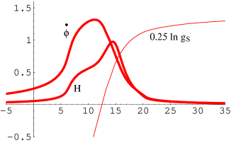
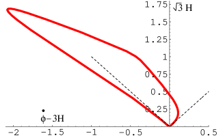
In addition, the perturbative approach at the two-loop level is self-consistent only for a quite small value of the final coupling, . A small value of the final dilaton, for the solutions of the action (8.69), seems to require, however, that and be both larger than and of the same order (in modulus) [149], in contrast with the usual expectation for the coefficients of a perturbative expansion.
If the string coupling is not kept small enough, on the other hand, the Universe necessarily enters the non-perturbative regime where typical M-theory effects may become important, as will be illustrated in Subsection 8.5. We shall first present, however, some arguments stressing the importance of the notion of entropy for a model-independent approach to the exit problem.
8.4 Graceful exit and entropy considerations
After the various models of exit reported in the previous subsections, it seems appropriate to recall, at this point, that entropy-related considerations have recently led to model-independent arguments in favour of the occurrence of a graceful exit in the pre-big bang scenario. As we shall see, those are physically quite close to the arguments based on backreaction and loop corrections, which we have already discussed.
Let us start by recalling that, as suggested by Bekenstein [73, 75], the entropy of a limited gravity system of energy and of size larger than its gravitational radius, , is limited by the upper bound
| (8.73) |
According to the holographic principle (see [376, 575] and references therein), on the other hand, the maximal entropy of a system is bounded by ,
| (8.74) |
where is the area of the space-like surface enclosing the region of space whose entropy we wish to bound. For systems of limited gravity, since and , the Bekenstein bound (8.73) implies the holography bound (8.74).
How can these bounds be extended to be applied to the whole Universe? At cosmological scales the Universe is not a system of limited gravity, since its large-distance behaviour is determined by the gravitational effect of its matter content through Friedmann’s equations. Furthermore, the holography bound obviously fails for sufficiently large regions of space since, for a given temperature, entropy grows like while area grows like . The generalization of entropy bounds to cosmology turned out to be subtle.
A possible prescription [74] for a cosmological extension is to identify in Eq. (8.73) with the particle horizon. In this way one can then arrive at the conclusion that the bound is violated sufficiently near the big-bang singularity, implying that the latter is fake (if the bound is always valid). More recently, a similar extension of the holographic bound to cosmology has been proposed [255], arguing that the area of the particle horizon should bound entropy on the backward-looking light cone, according to (8.74). It was soon realized, however, that the such a proposal requires modifications, since violations of it were found to occur in physically reasonable situations. An improvement of the proposal [255], applicable to light-like hypersurfaces, was later made by Bousso [97, 98] (see also [257]).
Of more interest, in our context, are however the attempts made at deriving cosmological entropy bounds on space-like hypersurfaces [232, 605, 49, 92, 393, 128]. These identify the maximal size of a spatial region for which holography works: the Hubble radius [232, 605, 393], the so-called apparent horizon [115], or, finally, a causal-connection (Jeans) scale [128].
For our purpose there is no need here to enter into the relative merits of these various proposals. Rather, we will only outline the physical idea behind them. Consider, inside a quasi-homogeneous Universe, a sphere of radius . We may consider “isolated” bodies, in the sense of Ref. [73], fully contained in the sphere, i.e. with radius . For such systems, the bound (8.73) holds, and it is saturated by a black hole of size . We may next consider several black holes inside our Hubble volume, each carrying an entropy proportional to the square of its mass. If two, or more, of these black holes merge, their masses will add up, while the total entropy after the merging, being quadratic in the total mass, will exceed the sum of the initial entropies. In other words, in order to maximize entropy, it pays to form black holes as large as possible.
Is there a limit to this process of entropy increase? The suggestion made in [232, 605, 49, 393, 128], which finds support in old results by several groups [148, 147, 506], is that a critical length of order is the upper limit on how large a classically stable black hole can be. If we accept this hypothesis, the upper bound on the entropy contained in a given region of space will be given by the number of Hubble volumes in , times the Bekenstein–Hawking entropy [72, 370] of a black hole of radius , . The two factors can be combined in the suggestive formula:
| (8.75) |
where is the volume of the space-like hypersurface whose entropy we wish to bound, and differs from one proposal to another, but is, roughly, of the order of the Hubble parameter. Actually, since is proportional to the trace of the second fundamental form on the hypersurface, Eq. (8.75) reminds us of the boundary term that has to be added to the gravitational action in order to correctly derive Einstein’s equations from the usual variational principle. This shows that the bound (8.75) is generally covariant for . It can also be written covariantly for the identification of made in [128].
For the qualitative discussion that follows, let us therefore take , and let us convert the bound to S-frame quantities, taking into account the relation between and , given in Eq. (1.25). We obtain [605]:
| (8.76) |
where we have fixed an arbitrary additive constant in the definition of . Equation (8.76) thus connects very simply the entropy bound of a region of fixed comoving volume to the most important variables occurring in string cosmology (see, e.g., the phase diagram of Fig. 8.1).
An immediate application of the bound (8.76) to the exit problem was pointed out in [605], noting that the bound is initially saturated in the E-frame picture of pre-big bang inflation as a collapse, with corresponding black-hole formation [130]. Since the entropy, and the bound itself, cannot decrease without a violation of the second law, one obtains:
| (8.77) |
It is easy to check that this relation holds with the equality sign during the initial, low-energy evolution from the string perturbative vacuum (see Eq. (8.5)). In other words, the Hubble entropy bound is saturated initially and throughout the low-energy, dilaton-driven evolution described in [130]. But what happens if the curvature stops its growth, (for instance, during the high-curvature string phase discussed in the previous subsections)? It is quite clear that Eq. (8.77) does not allow to reach saturation () in the upper-right quadrant of Fig. 8.1, since there. Instead, saturation of in the upper-left quadrant (where ) is perfectly all right. But this implies having attained the sought for branch change!
Let us now look at the loop corrections. Physically, these correspond to taking into account the backreaction from particle production, i.e. from the quantum fluctuations amplified by the cosmological evolution. Let us check when their entropy starts to threaten the bound. Using the results presented in [298, 299, 107, 108], the entropy density carried by quantum fluctuations inside a region of size is given by
| (8.78) |
where is the effective number of species that are amplified. This entropy equals the upper bound (8.76) precisely when
| (8.79) |
But this is also the line on which the energy density in quantum fluctuations is expected to become critical, and the backreaction of the produced radiation is expected to drive the Universe to the beginning of the standard radiation-dominated phase [276, 136].
Indeed, one can easily estimate the total energy stored in the quantum fluctuations amplified by the pre-big bang backgrounds (for a discussion of generic perturbation spectra, see [136, 120]). The result is, roughly,
| (8.80) |
where is the maximal curvature scale reached around the exit transition. The saturation of the entropy bound is thus equivalent to the condition that the above energy density becomes critical (and induces the exit) just around the transition scale . On the other hand, we have already argued that , and we know that, in heterotic string theory, is in the hundreds. It follows, according to this picture, that the exit may occur when the dilaton satisfies , i.e. at a value of the string coupling very close to its present one. The saturation of the Hubble entropy bound thus supports a picture in which the exit transition occurs to avoid violations of the (generalized) second law of thermodynamics, and it is induced by the backreaction of quantum fluctuations (see also [115] and the numerical examples of [150]).
Remarkably, this also explains why the radiation, which originates from the quantum fluctuations and dominates our final Friedmann phase, has an entropy that roughly corresponds to the number of elementary “Hubble spheres” (i.e. spatial regions of size ) contained inside our Universe just after the exit (namely, to the entropy of the quantum fluctuations evaluated at the string scale): . A very large number, on the one hand, but a very small entropy for the total mass and size of our present observable Universe, on the other hand, as often emphasized by Penrose [516]. The pre-big bang scenario may thus neatly explain why the Universe, at the big bang, looks so fine-tuned (without being so), and may provide a natural arrow of time in the direction of higher entropy [605].
In conclusion, the picture that finally emerges from all these considerations is best illustrated with reference to the diagram of Fig. 8.6. Two lines are shown, representing boundaries for the possible evolution. The horizontal boundary is forced upon by the large-curvature corrections, while the tilted line in the first quadrant corresponds to the equation that we have just discussed. This line was also suggested as a boundary beyond which copious production of -branes would set in [466] (see the next subsection). Thus, depending on initial conditions, the pre-big bang bubble corresponding to our Universe would hit first either the high-curvature or the large-entropy boundary and initiate an exit phase. Hopefully, a universal late-time attractor will emerge guiding the evolution into the FRW phase of standard cosmology.
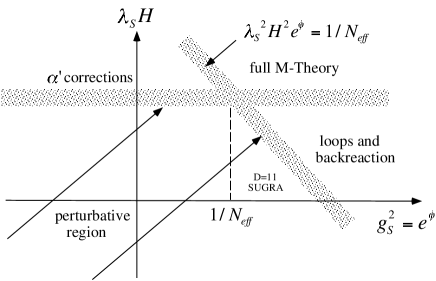
Needless to say, all these arguments have to be considered, at best, as having heuristic value. If we were to take them seriously, they would suggest that the Universe will never enter the strong-coupling, strong-curvature regime, where the largely unknown M-theory should be used. The low-energy limit of the latter (the much better understood supergravity) could suffice to deal with the fundamental exit problem of string cosmology. We refer to the next subsection for a short discussion of this possibility.
8.5 M-theory and brane cosmology
If the growth of the string coupling, which starts during the phase of accelerated pre-big bang evolution, is not stopped at some point by a dilaton potential (or by some other mechanism), the Universe necessarily enters the strong-coupling regime described by the so-called M-theory, which is well approximated, at low-energy, by the known supergravity theory [627]. In this subsection we will briefly report various ideas on the possibility of smoothing out the big bang singularity, and eventually implement the exit transition, in the context of the low-energy (i.e. small-curvature) limit of M-theory.
We start be recalling the action for the bosonic sector of eleven-dimensional supergravity,
| (8.81) | |||||
where is the field strength of the antisymmetric three-form potential , and the Chern–Simons term arises as a consequence of supersymmetry [187] (upper-case Latin indices run from to , Greek indices from to , and we follow the conventions of [88]. The ten-dimensional effective action, obtained by compactification of on a circle of radius (controlled by the dilaton [628]) can be written as
| (8.82) | |||||
where and are the field strengths of the antisymmetric potentials and , respectively, and we have dropped the one-form potential arising from the dimensional reduction of the metric. After the reduction, we have also rescaled the ten-dimensional metric as , and we have defined the ten-dimensional dilaton as .
The above action contains not only the usual string theory action, but also Ramond forms, i.e. higher-rank antisymmetric tensors uncoupled to the dilaton (in the S-frame), and exactly reproducing the Ramond–Ramond sector of the low-energy Type II A superstring action (see for instance [438]). This provides a new, in principle richer context to look for cosmological solutions [453, 392, 447, 184] (see [88] for a complete analysis of spatially flat models), suggesting also the possibility of an M-theory version of the pre-big bang scenario [152].
In such a context, the existence of black -brane solutions, of the type of those given in [70, 528], provides a first indication of a possible resolution of the problem of curvature singularities [427, 454] (see also [71] for examples including corrections). The different branches of a cosmological solution can indeed be related by -duality transformations [450], but an explicit representation of a smooth exit transition, in this context, is problematic [111]. By -duality it is possible, however, to transform a singular solution into a non-singular one (as in the case of -covariant backgrounds [309, 310]). This possibility has been studied, in particular, in the moduli space of supergravity compactified on a ten-torus [52].
In addition, the decompactification of the -th dimension, produced in the strong-coupling regime as a consequence of the identification of the string coupling with the -th dimensional scale factor [628, 377, 378], is possibly associated with a “softening” of curvature singularities, as pointed out in [394]. The study of some explicit examples has shown [250], in particular, that the curvature singularity of FWR models minimally coupled to a set of scalar fields, in four dimensions, can be removed by lifting the solutions to higher dimensions, provided the four-dimensional background has negative or vanishing spatial curvature (). In that case, the regular higher-dimensional backgrounds from which is obtained by dimensional reduction has only one of the extra dimensions that is dynamical, and for it coincides with the trivial Minkowski space-time parametrized by Milne coordinates.
A genuinely new effect, in the context of dimensionally reduced supergravity theories, is the presence of -branes, and the possibility of their production in the strong coupling regime where the brane states become light and (possibly) unstable. This effect might lead to regularizing the curvature singularities, as first proposed in some pioneering papers on string [428] and solitonic -brane [530] production in cosmological backgrounds. As suggested in [538], brane production might lead for instance to a phase of constant brane density, and then brane-driven (de Sitter) inflation (reminescent of the old idea of string-driven inflation [592]), thus freezing the growth of the background curvature. We should recall, finally, that brane production in high-energy scattering processes is also allowed for conventional Einstein gravity in models with large extra dimensions [8, 9].
More generally, as suggested in [466], when approaching the singularity one should describe the Universe not in terms of the metric and of the dilaton, but in terms of new low-energy modes, more appropriate to the strong-coupling regime where D(irichelet) -branes are the fundamental players. Indeed, in the string frame, their tension is controlled by , so that they are very light at strong coupling: for instance, a D-brane of type II A has a mass
| (8.83) |
In addition, they become unstable at large enough values of the Hubble parameter (an effect very similar to string instability in curved backgrounds [552, 315]), so that they can be copiously produced when approaching the singularity, and in particular around the epoch where [466] . As a consequence of this huge production, the D-brane energy density is expected to become critical, inducing a transition towards the standard radiation-dominated phase. If so, the curvature scale would be the largest value of curvature probed during the cosmological evolution [466].
More recently, the idea of a brane-dominated Universe has been further developed in the context of the so-called “brane gas cosmology” approach [11, 230] to the M-theory phase of the very early Universe (which generalised previous string-cosmology models [110, 583]). The Universe, in the strong-coupling regime, is assumed to have nine spatial dimensions in a toroidal topological state, and to be filled with a hot gas of -branes, with all modes in (approximate) thermal equilibrium. This approach aims not only at the resolution of the singularity problem, but also at providing a possible explanation of the number of spatial dimensions of our present Universe, along the lines of [110].
The model contains all the branes that appear in the spectrum of the (ten-dimensional) Type II A string theory. By recalling that M-theory contains the graviton (-brane), -branes and -branes as fundamental degress of freedom (see the action (8.81)), the compactification on a circle leads to -branes, strings (-branes), -branes, -branes, -branes, -branes and -branes (see Eq. (8.82)) as the fundamental extended objects of the -dimensional theory. The total action for the brane gas model is thus the sum of the low-energy effective action for the “bulk” (ten-dimensional) space-time manifold plus the ()-dimensional action of all the branes in the gas:
| (8.84) |
where is the gravidilaton–axion sector of the action (8.82); and the Born–Infeld action of a -brane, coupled to the bulk via delta function sources with strength fixed by the tension , is given by
| (8.85) |
Here is the induced metric on the brane, is the induced antisymmetric tensor, and is a gauge field possibly living on the brane.
All branes contribute to the energy of such a primordial gas with three types of modes [11]. There are winding modes, corresponding to -branes wrapping around cycles of the torus, momentum modes, corresponding to the centre-of-mass motion of the brane, and oscillatory modes, corresponding to fluctuations in the directions transverse to the brane. The brane action (8.85) can thus be expanded in terms of these modes, and by taking the average contribution of their stress tensor one obtains the effective “equation of state” for the gas of winding modes;
| (8.86) |
( is the pressure, the rank of the brane). The momentum modes have the “dual” equation of state (for strings, , one recovers the results of [315, 316]). Transverse oscillations can be viewed as particles living on the brane, and their equation of state is that of “ordinary” matter, with . It follows, from the covariant conservation of the stress tensor, that the energy of winding (w) modes increases with the scale factor as
| (8.87) |
(note, however, that should be included at very high temperature thermal corrections , and that this can modify the effective equation of state, as discussed in [342] for the case of strings near the Hagedorn scale).
The Universe, in the strong-coupling (M-theory) regime, is thus assumed to behave as a hot soup of all modes of all -branes. The curvature singularity is expected to be avoided because of -duality exchanging w-modes and momentum modes, and then transforming a phase of increasing temperature into decreasing temperature, with the fixed point of the symmetry acting as a regularizing cut-off for all physical observables [11, 230]. But the most interesting (and probably unique, at present) virtue of this scenario seems to be the possibility of explaining why our present Universe contains just three large spatial dimensions.
Indeed, as the primordial Universe expands, the w-modes tend to become dominant as their energy increases, starting with the largest value of , according to Eq. (8.87). The effect of the w-modes, on the other hand, is to halt the expansion [583], so that the spatial dimensions can decompactify (i.e. inflate away from the string scale) only if the w-modes disappear.
They can disappear by annihilation with antiwinding () modes (the initial number of w and is assumed to be the same, by symmetry). On the other hand, assuming that the space is periodic, it follows that the world-volume of two -branes will necessarily intersect in at most spatial dimensions. In the initial Universe , so that winding -branes with have no problem to self-annihilate. We are thus left with -branes and strings. The annihilation of the (heavier) winding -branes will first allow five dimensions to become large. Within this distinguished torus , the -branes (strings) w-modes will then only allow the subspace to expand.
In this way, one can understand the origin of the dimensionality of our Universe and, interestingly enough, can predict a hierarchical structure of the ten-dimensional compact manifold as follows [11]:
| (8.88) |
where comes from the original M-theory compactification on a circle, and the other compact manifolds have been listed in order of growing size, from left to right.
In this context, a possible problem is that, at the end of the decompactification process, at least one w-mode is left per Hubble volume, leading to the well known domain-wall problem. This problem can be solved if the w-modes, before they annihilate, drive the background to a phase of slight contraction, also called “loitering” [550], during which the Hubble horizon becomes larger than the spatial size of the Universe (as in the phase of pre-big bang inflation, when it is seen as a contraction in the E-frame).
By supplementing the string-cosmology equations by terms describing the annihilation of w-modes into string loops [104], it has been shown that during the loitering phase all w-modes are eliminated and that, from this point on, the Universe begins to expand again. The w-modes annihilation leads to breaking -duality, and it is tempting to speculate that this effect could be related to SUSY breaking, and to the mechanism of dilaton mass generation needed to stabilize the coupling after decompactification [104].
Outside the context of brane gas cosmology, but always in the context of an M-theory approach to the strong coupling regime, a more drastic resolution of the dimensionality problem is represented by the so-called brane-world scenario (inspired by heterotic M-theory [377, 378]), in which our Universe is assumed to coincide with a -brane embedded in a higher-dimensional bulk manifold [451, 452].
In a realistic picture, of course, our -brane is not expected to be the only extended object embedded in the bulk manifold, especially in the regime of large bulk dilaton, and very strong coupling. In that case, the transition to the post-big bang regime could be triggered by a head-on collision against another brane, just as happens in the context of the so-called “ekpyrotic” scenario [413, 414], where the big bang explosion, and the birth of a hot, radiation-dominated Universe, is simulated by the collision of two -branes along a (hidden) fifth spatial dimension (see also [326] for a similar but spherically symmetric process of bubble collision).
In the ekpyrotic scenario the -th space-time is assumed to have topology , with two branes at the orbifolds fixed points, where space-time has boundaries. Six dimensions are compactified on a Calabi–Yau threefold, leaving the effective theory five-dimensional. The boundary branes are called the visible and the hidden brane, the visible one being identified with our Universe.
The action for this model is the sum of three parts:
| (8.89) |
where represents the brane interactions, describes the matter on the brane created by the collision, and is the action of five-dimensional heterotic M-theory. With the conventions of [413]:
| (8.90) |
Here is the five-dimensional Planck mass, is the field strength of the four-form , is the induced metric on the -th -brane, whose embedding in five dimensions is described by the five parametric equations . Finally, the tensions are given by .
In the first version of the ekpyrotic scenario [413], besides the two boundary branes, there is a third “bulk” brane, possibly originated from spontaneous bubble nucleation. In that case, the three tensions satisfy the condition , with and , and the bulk brane is attracted towards the visible brane, until they collide. The kinetic energy of the bulk brane is then converted into matter and radiation of the visible brane, with a spectrum of density perturbations left impressed by the quantum fluctuations of the bulk brane.
In the second version of the scenario [414], there are instead only the two boundary branes, which collide and then bounce apart, in what is hoped to be a non-singular process. This second possibility also represents an important ingredient in a related, recently proposed “cyclic” model of Universe [574].
In our context, this second possibility is particularly interesting because the collision of the two boundary branes is associated to the collapse of the dimension transverse to the brane: namely, of the -th dimension, taking into account the Calabi-Yau compactification. But the shrinking of the eleven-dimensional radius , in an M-theory context, is equivalent to a decreasing of the string coupling (recall that ). This means that the collision, and the subsequent beginning of the radiation-dominated, post-big bang evolution, occurs at very weak coupling, in the perturbative regime.
In conclusion, this model suggests that the space-time manifold, after having reached the strong-coupling, M-theory regime as a consequence of the pre-big bang evolution, and after the associated production of branes, might be forced again to the perturbative regime by the attraction (and by the subsequent collapse) of the branes at the boundary of the space-time. The exit would thus proceed at weak coupling (possibly with a mechanism of radiation production different from the one discussed in the previous subsections). This may perhaps justify the use of the tree-level effective action for the quantum cosmology approach to the exit, presented in the next section.
9 Quantum string cosmology
According to the pre-big bang scenario, the present cosmological state of our Universe should emerge as the result of a long evolution, starting from the string perturbative vacuum. Such an evolution necessarily includes the transition from a phase of growing curvature and strong coupling to a phase of decreasing curvature and (nearly) constant string coupling. The full dynamical description of such a process still contains various problematic aspects, as discussed in the previous section.
Since the transition is expected to occur in the high-curvature (nearly Planckian) regime, where quantum-gravity effects may become important, it is not excluded that a quantum-cosmology approach may be appropriate to describe the “decay” of the string perturbative vacuum into our present, post-big bang Universe. Also in the context of the standard inflationary scenario, in fact, the quantum-cosmology approach is required to describe the “birth” of our classical Universe out of the Planckian regime [614]. With an important difference, however: in the standard scenario the initial state of the Universe is unknown, and has to be fixed through some ad hoc prescription. There are various possible choices for the initial boundary conditions [367, 371, 610, 441, 634, 542, 612], leading in general to different quantum pictures of the early cosmological evolution. In the pre-big bang scenario, on the contrary, the initial state is fixed in such a way as to approach, asymptotically, the string perturbative vacuum, and this unambiguously determines the initial wave function.
In a quantum cosmology context the Universe is described by a wave function evolving in superspace, according to the Wheeler–De Witt (WDW) equation [217, 623], and it is always possible, in principle, to compute the transition probability between two different geometrical configurations –in particular, from a pre- to a post-big bang state. We shall report here the results obtained in the context of what may be called a “low-energy” approach to quantum-string cosmology [283], which is based on the lowest-order string effective action, and in which no higher-order ( and loop) corrections are taken into account into the WDW equation, except those possibly encoded into an effective, non-perturbative dilaton potential (see [526, 527, 553] for high-curvature contributions to the WDW equation).
Such a low-energy approach, first introduced in string cosmology in [144, 80, 435], is analogous (in the particle case) to low-energy quantum mechanics, where one neglects relativistic and higher-order corrections. It is a first approximation, which is already sufficient to take into account pure quantum-gravity effects, such as the possibility of transitions which are classically forbidden –in particular, transitions between two low-energy geometric configurations which are classically disconnected by a singularity [311, 323, 155]– and thus to motivate a “minisuperspace approach” to the exit problem [280] (see also [475, 512] for a recent quantum-cosmology approach to this problem based on the Bohm–de Broglie ontological interpretation of quantum mechanics).
Quite irrespectively of its applications, quantum-string cosmology may represent a rich and interesting field of research in itself; it thus seems appropriate to recall that it is affected by various conceptual problems already present in the “standard” quantum-cosmology context: the meaning of the probabilistic interpretation [611], the existence and the meaning of a semiclassical limit [80, 435], the unambiguous identification of the time-like coordinate (see however [153]). Other problems affecting the standard scenario, however, disappear. In particular, in the context of the pre-big bang scenario, there is no problem of boundary conditions, which are unambiguously prescribed by the choice of the string perturbative vacuum (see Subsection 9.2); no problem either of operator ordering in the WDW equation (see for instance [37]), as the ordering is fixed by the duality symmetry of the string effective action [311, 411]. This important property of quantum-string cosmology will be illustrated in the next subsection.
9.1 The Wheeler–De Witt equation
The simplest example of quantum-string cosmology model is based on the lowest-order, gravidilaton string effective action
| (9.1) |
where we have included a (possibly non-local and non-perturbative) dilaton potential (see [154] for more complete models based on the M-theory action). If we are considering, in particular, an isotropic and spatially flat cosmological background,
| (9.2) |
the gravidilaton system has only two physical degrees of freedom, the scale factor and the dilaton (the “lapse” function can be arbitrarily fixed by a choice of gauge). The quantum evolution of the system is thus associated to a two-dimensional “minisuperspace”, which, assuming spatial sections of finite volume, can be conveniently parametrized by
| (9.3) |
Each “point” of the minisuperspace will then represent a classical solution of the action (9.1).
In terms of the coordinates of the minisuperspace, the action (after integration by parts) can be explicitly written as
| (9.4) |
Its variation with respect to defines the total energy density of the gravidilaton system, and leads to the so-called Hamiltonian constraint (in the cosmic time gauge, ):
| (9.5) |
Introducing the canonical momenta
| (9.6) |
the Hamiltonian constraint becomes
| (9.7) |
and its differential implementation in the minisuperspace spanned by and finally leads to the WDW equation for the gravidilaton system:
| (9.8) |
It is important to stress that such an equation is manifestly free from operator-ordering problems, as the Hamiltonian (9.7) has a flat metric in momentum space. This is not a special feature of the case we have considered because, thanks to the duality symmetry of the string effective action, the associated WDW minisuperspace is globally flat, and we can always choose a convenient parametrization leading to a flat minisuperspace metric.
For a more general discussion of this point we may add to the effective action (9.1) a non-trivial antisymmetric tensor background, . The kinetic part of the action may then be written in compact form as [311, 411] (see Subsection 2.3):
| (9.9) |
where , and is a symmetric matrix, including the spatial part of the background fields, , , and already defined in Eq. (2.55). We recall that this action is invariant under global transformations that leave the shifted dilaton invariant,
| (9.10) |
where
| (9.11) |
The Hamiltonian associated to torsion-graviton background,
| (9.12) |
would seem to have ordering problems, because . However, thanks to the properties of ,
| (9.13) |
we can always rewrite the kinetic part of the action in terms of the flat metric :
| (9.14) |
The corresponding Hamiltonian
| (9.15) |
has a flat metric in momentum space, with no ordering problems for the corresponding WDW equation [311, 411]:
| (9.16) |
On the other hand, if we insist on adopting a curvilinear parametrization of the minisuperspace, the ordering fixed by the duality symmetry is exactly the same as the ordering imposed by the requirement of reparametrization invariance, as there are no contributions to the ordered Hamiltonian from the scalar curvature of minisuperspace [37], because minisuperspace is globally flat.
To illustrate this point we may consider the pair of minisuperspace coordinates , different from the previous pair used in Eq. (9.4). The kinetic part of the action (9.1) then leads to the (kinetic part of the) Hamiltonian
| (9.17) |
where
| (9.18) |
corresponding to the non-trivial metric:
| (9.19) |
The quantum operator associated to the Hamiltonian (9.17) has to be ordered, because , and its differential representation can be written in general as
| (9.20) |
where is a c-number parameter depending on the ordering. Note that there are no contributions to the ordered Hamiltonian from the minisuperspace scalar curvature [37], which is vanishing for the metric (9.19).
Reparametrization invariance now imposes on the Hamiltonian the covariant d’Alembert form
| (9.21) |
and consequently fixes . The kinetic part of the action (9.4), on the other hand, is invariant under the -duality transformation [600, 581]
| (9.22) |
which implies, for the Hamiltonian (9.20),
| (9.23) |
The invariance of the Hamiltonian requires , and thus fixes the same quantum ordering as the condition of general covariance in minisuperspace. A similar relation between quantum ordering and duality symmetry can be easily established for more general effective actions, including a larger class of non-minimal gravidilaton couplings [435, 436].
9.2 Wave scattering in minisuperspace
In the absence of dilaton potential, the WDW equation (9.8) reduces to the free d’Alembert equation and provides a plane-wave representation in minisuperspace of the different asymptotic branches of the classical solutions.
Let us recall, in fact, that the solutions of the low-energy effective action (9.4) always contain four branches. For , in particular, we have four (physically different) solutions,
| (9.24) |
related by the duality transformation (9.22) and by time reversal, . They satisfy the condition
| (9.25) |
and may thus be represented as the bisecting lines of the plane , corresponding to
-
•
expansion ,
-
•
contraction ,
-
•
pre-big bang (growing dilaton) ,
-
•
post-big bang (decreasing dilaton) ,
as illustrated in Fig. 9.1. We may note, for later use, that if we add to the action a positive cosmological constant (), then the classical solutions are represented in the plane by the hyperbolas
| (9.26) |
In that case, the initial configuration is shifted to a state with flat metric and linearly evolving dilaton, but the solution is still characterized by four branches coinciding, asymptotically, with the free configurations of Eq. (9.24).
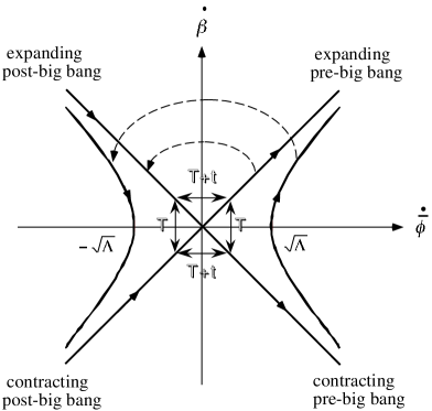
The solutions of the WDW equations, on the other hand, can be factorized in the form of plane waves representing free energy and momentum eigenstates:
| (9.27) |
where ():
| (9.28) |
By recalling that , (see Eq. (9.6)), the above plane waves represent the four branches of Eq. (9.24), defined by , with the following correspondence:
-
•
expansion ,
-
•
contraction ,
-
•
pre-big bang (growing dilaton) ,
-
•
post-big bang (decreasing dilaton) .
For an isotropic, low-energy solution [600], the dilaton is growing () only if the metric is expanding (), see Eq. (9.3). If we impose, as our physical boundary condition, that the Universe emerge from the string perturbative vacuum (corresponding, asymptotically, to , ), then the initial state must represent a configuration with positive eigenvalue of and opposite eigenvalue of , i.e. (see also [190] for a detailed discussion of boundary conditions in quantum-string cosmology).
A quantum transition from pre- to post-big bang thus becomes, in this representation, a transition from an initial state
| (9.29) |
to a final state
| (9.30) |
(see the dashed curves of Fig. 9.1). The associated trajectory describes a monotonic evolution along , and a reflection along . The above discussion suggests that we look at the quantum evolution (in minisuperspace) of the initial pre-big bang state as at the scattering, induced by an effective WDW potential, of an incoming wave travelling from along the positive direction of the axes and .
The effective potential, on the other hand, is known to be strongly suppressed as we approach the string perturbative vacuum, . We shall assume that a possible growth of in the strong-coupling regime is not strong enough to prevent the effective WDW potential from going to zero also at large positive values of and , so that for . It follows that also the final asymptotic configuration can be represented by the free eigenstates . However, even if the initial state is fixed by the boundary conditions of the pre-big bang scenario, the final state is not, and there are in general four different types of evolution [283], depending on whether the asymptotic outgoing state is a superposition of waves with the same and opposite , or with the same and opposite , and also depending on the identification of the time-like coordinate in minisuperspace [153, 155].
These four possibilities are illustrated in Fig. 9.2, where cases and correspond to , while cases and correspond to . Also, in cases and the time-like coordinate is identified with , in cases and with . It must be noted that cases and require a duality-breaking dilaton potential, otherwise , and then a reflection along the axis is impossible, even at the quantum level [311].
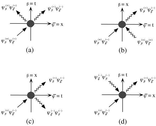
The two cases and represent scattering and reflection along the spacelike axes and , respectively. In case the evolution along is monotonic, so that the Universe always keeps expanding. The incident wave is partially transmitted towards the pre-big bang singularity (unbounded growth of the curvature and of the dilaton, , ), and partially reflected back towards the low-energy, expanding, post-big bang regime (, ) [311]. In case the evolution is monotonic along the time axis , but not along . The incident wave is therefore totally transmitted towards the singularity (), but in part as an expanding configuration and in part as a contracting one333R. Ricci, M. Gasperini and G. Veneziano (1996), unpublished..
The other two cases, and , are qualitatively different, as the final state is a superposition of positive and negative energy eigenstates, i.e. of modes of positive and negative frequency with respect to the time axes chosen in minisuperspace. In the language of third quantization [543, 422, 358, 359, 360] (i.e. second quantization of the WDW wave function in superspace) they represent a “Bogoliubov mixing”, describing the production of pairs of universes from the vacuum. The mode moving backwards in time has to be “re-interpreted”, as in quantum field theory, as an “antiuniverse” of positive energy and opposite momentum (in superspace). Since the inversion of momentum, in superspace, corresponds to a reflection of , the re-interpretation principle in this context changes expansion into contraction, and vice versa.
Case , in particular, describes the production of universe–antiuniverse pairs –one expanding, the other contracting– from the string perturbative vacuum [131]. The pairs evolve towards the strong-coupling regime , so that both members of the pair fall inside the pre-big bang singularity. Case is more interesting, in our context, since there the universe and the antiuniverse of the pair are both expanding: one falls inside the pre-big bang singularity, the other expands towards the low-energy, post-big bang regime, and may expand to infinity, representing the birth of a Universe like ours in a standard Friedmann-like configuration [291].
Possible explicit examples of a quantum representation in minisuperspace of the transition from pre- to post-big bang, based on the above scattering processes, will be given in the next two subsections.
9.3 Birth of the Universe as “quantum reflection”
The simplest way to represent the transition from the string perturbative vacuum to the present, post-big bang regime, is to identify the time-like coordinate in the minisuperspace with , and to represent the process as a reflection of the incoming wave function along the space-like coordinate , according to Eqs. (9.29), (9.30) (case of Fig. 9.2). The transition probability is thus controlled by the reflection coefficient
| (9.31) |
where are the asymptotic components of the WDW wave function at , containing the left-moving and right-moving part of the wave along (see [153] for a rigorous definition of scalar products in the appropriate Hilbert space, and [155, 156, 340] for a path-integral approach to the computation of the transition amplitudes).
Without potential in the WDW equation there is no transition, of course (in the absence of a dilaton potential, the possible decoherence of the quantum-cosmological system, and its implications for the exit problem, have been discussed in [455]). With an appropriate potential, allowing a smooth classical evolution from pre- to post-big bang, the transition probability tends to unity; may be non-zero, however, even if the two branches of the classical solution are causally disconnected by a singularity.
An instructive example, to this purpose, is provided by the duality-symmetric (non-local) four-loop dilaton potential
| (9.32) |
already introduced in Subsection 8.1 (for generalized exponential potential, with the inclusion of the antisymmetric tensor contribution to the WDW equation, see [468]). The corresponding action (9.4), in , has the following classical solution [311]
| (9.33) |
where is an integration constant, and
| (9.34) |
is the conserved momentum along the axis.
For , Eq. (9.33) describes a regular “self-dual” solution –satisfying – characterized by a “bell-like” shape of the curvature scale and of the coupling (see Subsection 8.1). The solutions of the WDW equation (9.8), in the small coupling regime , can be written as [311]
| (9.35) | |||||
( is a normalization coefficient), and contain the superposition of the initial string perturbative vacuum and of the reflected component, representing the post-big bang regime. Clearly, for all , as the two branches of the solution are smoothly connected already at the classical level.
For , on the contrary, the pre- and post-big bang branches are disconnected by an unphysical region, of extension , where the expansion rate and the dilaton coupling become imaginary. Such a region is bounded, on both sides, by a curvature singularity. However, after fixing the boundary conditions with the string perturbative vacuum and in the small coupling regime, the solutions of the WDW equation can be written as [311]:
| (9.36) | |||||
The reflection coefficient
| (9.37) |
is exponentially suppressed but non-zero, corresponding to a non-vanishing transition probability from the pre- to the post-big bang branches of the above solution.
Exactly the same result (9.37) is obtained for the simplest case of dilaton potential, a positive cosmological constant . In that case, by expressing the conserved momentum in terms of the coupling at the string scale , the transition probability between the left and right branches of the hyperbolas of Fig. 9.1, for a three-dimensional portion of space of fixed proper volume at , can be written in the form [323]:
| (9.38) |
Unfortunately, such a transition probability is exponentially suppressed, unless the proper size of the transition volume is small, and the cosmological constant is large, in string units. Note, however, that the probability is peaked in the string coupling regime, with a typical “instantonic” behaviour : this means that the Universe tends to emerge from the transition in the coupling regime appropriate to the present post-big bang phase.
It is important to stress that the quantum-transition probabilities (9.37), (9.38) have a conceptual meaning different from similar results obtained in the context of the standard inflationary scenario. In string cosmology, in fact, the quantum (Planckian) regime is reached at the end of the pre-big bang phase, when the Universe is expected to exit from (not to enter in) the inflationary regime. Thus, quantum effects are not responsible for inflationary initial conditions [287], whereas they are in the standard inflationary scenario [395]. In spite of this important difference, the result (9.37) is formally very similar to the probability that our Universe may emerge from the Planckian regime obtained in the context of the “tunnelling from nothing” and other similar inflationary scenarios [10, 610, 441, 634, 542], where the probability is also exponentially suppressed, and the coefficient is inversely proportional to the effective cosmological constant and to the gravitational coupling, .
The reason for this formal analogy is easy to understand if we recall that, by choosing the string perturbative vacuum as the initial state of the pre-big bang scenario, it follows that in minisuperspace there are only right-moving waves approaching the singularity at . This is exactly equivalent to imposing tunnelling boundary conditions that select only outgoing modes at the singular space-time boundary [611, 612].
In this sense, the quantum reflection illustrated in this subsection can also be interpreted as a tunnelling process, not “from nothing”, however, but “from the string perturbative vacuum”. A different minisuperspace representation of the birth of the Universe from the vacuum will be illustrated in the next subsection.
9.4 Birth of the Universe as “antitunnelling”
The process of quantum reflection (or tunnelling) is not the only “channel” open to vacuum decay in the string cosmology minisuperspace introduced in the previous subsections. There are also other –in principle more efficient– processes, such as the parametric amplification of the WDW wave function, which could represent the transition to our present cosmological state. We refer, in particular, to the cases and illustrated in Fig. 9.2.
Case , discussed in [131], shows indeed that a primordial conversion of expanding into contracting dimensions, corresponding to the production of pairs of Universes from the vacuum, can be efficiently described as the parametric amplification of the wave function. In this subsection we shall report a particular, explicit example of case [291] to show that, with an appropriate model of dilaton potential, the parametric amplification of the wave function can also efficiently represent the transition from the pre- to the post-big bang regime, via pair production from the vacuum. In that case, the birth of the Universe can be described as a process of “antitunnelling from the string perturbative vacuum” (the term “antitunnelling”, synonymous of parametric amplification, follows from the fact that the transition probability in that case is controlled by the inverse of the quantum-mechanical transmission coefficient, see Subsection 4.4).
First of all we note that, with a duality-invariant dilaton potential, the string-cosmology Hamiltonian is translationally invariant along the axis: in that case, the initial expanding pre-big bang configuration keeps expanding, and the out state cannot be a mixture of states with positive and negative eigenvalues of . To implement the process of Fig. 9.2, we thus need a non-local, duality-breaking potential, which contains both the metric and the dilaton, but not in the combination . We shall use, in particular, a two-loop dilaton potential induced by an effective cosmological constant (two-loop potentials are known to favour the transition to the post-big bang regime already at the classical level [320, 123], but only for appropriate repulsive self-interactions, ). We shall assume, in addition, that such a potential is rapidly damped in the large-radius limit , and we shall approximate such a damping, for simplicity, by the Heaviside step function , by setting
| (9.39) |
With such a damping we represent the effective suppression of the cosmological constant, required for the transition to a realistic post-big bang configuration.
Given the above potential, the general solution of the WDW equation can be factorized in terms of the eigenstates of the momentum , by setting
| (9.40) |
In the region the potential is vanishing, and the outgoing solution is a superposition of eigenstates of corresponding to positive and negative frequency modes , as in case of Fig. 9.2. In the region the solution is a combination of Bessel functions , of imaginary index and argument . If we fix the boundary conditions at , by imposing that the Universe starts expanding from the string perturbative vacuum,
| (9.41) |
then the WDW wave function is uniquely determined as:
| (9.42) |
With the matching conditions at we can finally compute the Bogoliubov coefficients determining, in the third quantization formalism, the number of universes produced from the vacuum, for each mode (where represents a given configuration in the space of the initial parameters).
As shown by an explicit computation [131, 291], the wave function is parametrically amplified (i.e. ), for all . In that case, the birth of our present post-big bang Universe may proceed efficiently, and may be represented in minisuperspace as the forced production of pairs of Universes from the quantum fluctuations of the string perturbative vacuum. However, for a realistic process occurring at the string scale, with and , the condition of parametric amplification can be written as
| (9.43) |
where is the proper spatial volume emerging from the transition in the post-big bang regime. This implies that the transition is strongly favoured for configurations of small enough spatial volume in string units, large enough coupling , and/or large enough cosmological constant (in string units), just as in the cases discussed in the previous subsection.
For the wave function does not “hit” the barrier, there is no parametric amplification, and the inital state runs almost undisturbed towards the singularity. Only a small, exponentially suppressed fraction is able to emerge in the post-big bang regime, exactly as in the case of tunnelling (or quantum reflection). In the context of third quantization, this process can still be described as the production of pairs of universes, but the number of pairs is now exponentially damped, , with a Boltzmann factor corresponding to a “thermal bath” of universes, at the effective temperature in superspace.
It seems possible to conclude, therefore, that the low-energy quantum-cosmology processes considered in this subsection may allow a quantum transition from pre- to post-big bang configurations, even if such configurations are classically disconnected. With a “realistic” dilaton potential, the “bubbles” of post-big bang phase nucleated out of the string perturbative vacuum seem, however, to be too small to reproduce our present Universe without a further long period of post-big bang inflation. The quantum processes reported in this Section, however, could explain the “foam” of infinitely many “baby Universes” required, for instance, in the context of chaotic inflation [443] and of other, standard, inflationary scenarios.
10 Conclusion
In this last section we will conclude our report by discussing a possible “late-time” consequence of the pre-big bang scenario –the large-scale dominance of the dilatonic dark energy density– and by presenting a list of various problems and aspects of such a scenario that are not included in the previous sections. Finally, we will summarize our personal outlook of string cosmology, together with some speculations about its possible future perspectives.
10.1 Towards the future: a dilaton-dominated Universe?
The dilaton is, undoubtedly, one of the most important ingredients of the pre-big bang scenario illustrated in this paper. Indeed, the dilaton implements the duality symmetry, controls the strength of all interactions, sustains the initial inflationary evolution, contributes to the amplification of the quantum fluctuations (and, in particular, to the production of seeds for the magnetic fields), leading eventually to the formation of a cosmic background of massive scalar particles. All such effects are typical of string cosmology and represent the “imprint” of the pre-big bang scenario with respect to other, more conventional, inflationary scenarios.
Not satisfied with all such effects, however, the dilaton could still be hale and hearty, and still in action even today, so that it would affect in a determinant way not only the very early cosmological past, but also the present (and, possibly, future) state of our Universe. The dilaton potential energy, or a mixture of kinetic and potential energy density, could represent in fact the dark component responsible for the cosmic acceleration observed very recently [536, 517]. In this sense, string theory can automatically provide, with the dilaton, a “non-minimal” model of quintessence [294, 312] (i.e. a model of quintessence based on a scalar field non-minimally coupled to gravity and to elementary matter fields).
There are, basically, two possible scenarios, depending on the (currently uncertain) shape of the non-perturbative dilaton potential . In the context of superstring models for grand-unified theories (GUTs), the present value of the dilaton should determine in fact the whole set of gravitational and gauge coupling parameters, which are today constant (or, if they are time-dependent, are nevertheless running very slowly on a cosmological time scale). This constraint can be implemented in two ways.
The first possibility is a dilaton almost frozen at a minimum of the potential, in the moderate-coupling regime with of order , in such a way that the GUT gauge coupling is fixed to [404]
| (10.1) |
The second possibility is a dilaton monotonically running towards , and the couplings saturated at small values in the strong-coupling regime because of the large number of fields entering the loop corrections, or the large value of the quadratic Casimir for unification gauge groups like . Realistic values of and can be obtained at , for , typically as [607, 608]:
| (10.2) |
In both cases, if the present value of the potential is of the order of the present Hubble scale (and, possibly, ), the dilaton can reproduce the observed “dark-energy” effects, playing the role of the so-called “quintessence” [139]. The required fine-tuning of the amplitude of the potential (and the corresponding ultra-light value of the dilaton mass, ), seems to be unavoidable. In this context, however, it seems possible to alleviate the problem of the “cosmic coincidence” [573], generated by the observed (approximate) equality , where is the present energy density of the dominant dark-matter component. Let us explain how this could happen, in both the weak-coupling and the strong-coupling scenarios of dilatonic quintessence.
In the first case we note that, even assuming that the dilaton gets frozen at a value after the transition to the post-big bang regime, with a potential energy that is initially negligible (), it may keep frozen for the whole duration of the radiation epoch, but it tends to be shifted away from equilibrium as soon as the Universe enters the matter-dominated regime.
Suppose in fact that we add a potential to the low-energy gravidilaton action:
| (10.3) |
where describes, for simplicity, perfect-fluid sources minimally coupled to the background. For a homogeneous and conformally flat metric, the dilaton equation can then be written in the form
| (10.4) |
Combining this equation with the standard conservation equation of the matter sources,
| (10.5) |
it follows that constant and stable solutions (with ) are allowed in three cases only: 1) vacuum, , ; 2) cosmological constant, const, const; 3) radiation, , .
So, even if the dilaton is “sleeping” in the radiation era, it “wakes up” and starts rolling away from the freezing position determined by just after the equilibrium epoch. We are thus led to the following question: For which values of the potential may the dilaton bounce back to the minimum, and the matter era be followed by a quintessential, potential-dominated epoch?
If the answer would point only and precisely at , then the cosmic coincidence would be explained. If the answer would indicate for a restricted range of values, including , the coincidence problem would remain, but it would be alleviated.
The answer to the above question depends on the shape of the potential, and on the effective strength of the dilaton coupling to macroscopic matter. To illustrate this point we may consider the E-frame cosmological equations (6.2), obtained from the action (10.3) through the conformal transformation
| (10.6) |
In units of (and omitting the tilde, for simplicity), the dilaton equation becomes
| (10.7) |
where we have taken into account, through the coupling function , a possible loop renormalization of the effective dilaton coupling in the matter action. In the radiation era, and a stable, frozen dilaton () thus corresponds to an extremum of the E-frame potential, . In the matter era, when , there is a dilaton acceleration away from the minimum, , possibly contrasted by the restoring force .
Consider now a typical, supersymmetry-breaking dilaton potential, instantonically suppressed [90] at , with a non-trivial structure developing a minimum in the region of moderate coupling, and exponentially growing at because of the conformal transformation to the E-frame. A “minimal” example of such a potential can be simply parametrized (in the E-frame) as follows [399]
| (10.8) |
where are dimensionless numbers of order For an illustrative purpose we will choose here the particular values , , , in such a way that the minimum is at , and that , in agreement with Eq. (10.1).
With the above choice of parameters, the dilaton potential is plotted in Fig. 10.1 for different values of . It is important to note that the extremum is not separated from the perturbative regime () by an infinite potential barrier, and that the lower , the lower the barrier, the weaker is the restoring force and the easier it is for the dilaton to escape from the minimum and run to .
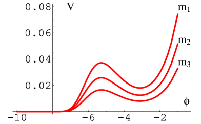
To match present phenomenology, the value of , in such a context, has to be chosen very small in string units, (see below for a possible justification). It follows that the potential barrier is very low, and the dilaton would certainly escape from the minimum at the beginning of the matter era, unless the coupling to matter () is also correspondingly small. Such a coupling, on the other hand, has to be very small, because the corresponding scalar force has a very long range, , and the dilaton must be strongly decoupled (, at least today) to avoid unacceptable violations of the equivalence principle [198, 199].
It can be shown, as a consequence, that the present values of allowed by the gravitational phenomenology () are compatible with a late cosmological phase dominated by the dilaton potential only for a restricted range of , which depends on the value of at the equilibrium epoch, [294]. Expanding around the minimum, and starting from , for instance, a numerical analysis shows that the dilaton, after a small shift at the equilibrium epoch, bounces back to the minimum provided , which includes the realistic case . In such a context, therefore, the coincidence problem is not strictly solved, but possibly alleviated (see [294] for a more detailed discussion).
An alternative scenario for a dilatonic interpretation of the observed “quintessential” effects, is based on the assumption that the dilaton never gets trapped in a minimum, and evolves monotonically (and boundlessly) from negative (pre-big bang) to positive (post-big bang) values, with a potential smoothly approaching zero as (see Fig. 2.1). The non-perturbative potential, in this context, is typically characterized by a bell-like shape, which can be parametrized (in the S-frame) as [312]:
| (10.9) |
where are dimensionless numbers of order unity and, again, the mass scale satisfies , to avoid that the dilaton becomes dominant too early.
As before, the potential is instantonically suppressed at , but now is also esponentially suppressed in the limit. The mass scale , in the context of a non-perturbative potential, is naturally related to the string scale by , where is a model-dependent parameter of order . This may explain the smallness of the potential in string units, but it should not hide the fact that the constant parameter has to be precisely adjusted ad hoc if we want to start the accelerated dilaton-dominated phase not much earlier than at redshifts of order one [588], and not later than today.
In the context of a running-dilaton scenario, the gauge couplings and the ratio are to be stabilized, in the limit, by the loop corrections. Such corrections, on the other hand, also play a fundamental role in determining the effective dilatonic charge of the elementary fields appearing in the matter action. Thanks to this interplay, a dilatonic charge that switches on at late times, in the (non-baryonic) dark-matter sector, seems able to provide a possible dynamical explanation of the cosmic coincidence [312] (see [196, 197] for possible related violations of free-fall universality, and time variation of the natural constants, induced in this context).
Such a dynamical approach to the coincidence problem is based, in particular, on the following loop-corrected action
| (10.10) |
where is the potential of Eq. (10.9), and the loop form factors and , in a minimal “induced-gravity” scenario, are assumed to be parametrized at large as follows [607, 608]:
| (10.11) |
where , in agreement with Eq. (10.2). We also assume that the action contains non-baryonic dark-matter whose dilatonic charge density per unit of gravitational mass, , switches on as , and can be parametrized as [312]:
| (10.12) |
where, again, . Note that we are using here a definition of dilatonic charge density different from the one previously introduced in Eqs. (6.16) and (8.41).
The analytical and numerical study of such a model shows that, in a way that is largely independent from the initial conditions, the Universe is eventually driven to an asymptotic accelerated regime characterized by a frozen ratio between the dark-matter and the dilatonic energy density, const. The present approximate equality of and is no longer a coincidence, in this context, but a dynamical property of the asymptotic configuration, as in models of “coupled quintessence” [374, 27].
For a better illustration of the “late-time” post-big bang scenario, described by Eqs. (10.10)–(10.12), it is convenient to consider the E-frame cosmological equations for the tilted variables defined through the conformal transformation
| (10.13) |
(we are considering, as before, perfect-fluid sources evolving in a conformally flat metric background). Note that , according to Eq. (10.11), controls the asymptotic value of the ratio between the string and the Planck scale, . The E-frame equations thus become (omitting the tilde, and in units ) [312]
| (10.14) | |||
| (10.15) | |||
| (10.16) |
where a dot denotes differentiation with respect to the E-frame cosmic time, and we have defined:
| (10.17) | |||
| (10.18) |
The source terms generically include the contribution of radiation, baryonic and non-baryonic matter components, but only for the non-baryonic dark component is the dilaton charge assumed to be significantly different from zero, and parametrized as in Eq. (10.12). By analysing the time evolution of the (total) dilaton energy density, , we then find that the post-big bang solutions are generally characterized by three dynamical phases [312].
Suppose in fact that the radiation-dominated, post-big bang regime starts with with a negligible dilaton potential, a negligible dark-matter energy density , and a fully kinetic dilaton energy density ,which is rapidly diluted as . When falls below one finds that the Universe enters a first “focusing” phase with , so that the dilaton kinetic energy starts growing with respect to radiation, and converges towards the other energy components.
When the matter becomes dominant, the Universe enters a subsequent “dragging” phase, where and evolve in time with the same behaviour, together with the baryonic matter density (uncoupled to the dilaton), . Actually, and are diluted a little bit faster (like ) than , but the deviation is controlled by a parameter, which is constant and very small during the dragging phase,
| (10.19) |
At late times (but not later than today) the potential and the dilaton charge of dark-matter come eventually into play, and the Universe enters a “freezing” phase characterized by a constant ratio , and by accelerated evolution. In this asymptotic regime, , the parameters of the model approach the constant values
| (10.20) |
and the E-frame equations can be written as
| (10.21) | |||
| (10.22) |
where
| (10.23) | |||
| (10.24) |
They can be solved by an asymptotic configuration with constant , and (acting as late-time attractor [25]), where the dilaton fraction of critical energy density, , the dilaton equation of state, , and the asymptotic acceleration parameter, are given by [312]
| (10.25) | |||
| (10.26) |
Such an asymptotic configuration is illustrated in Fig. 10.2, where we have plotted various curves at const and const in the plane. As shown in the figure, a positive acceleration () is perfectly compatible with the range of and allowed by present phenomenological constraints [618, 50], namely and .
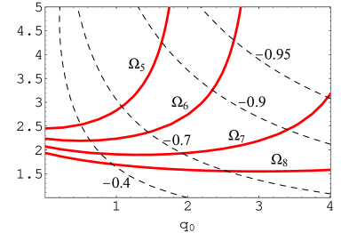
We note, finally, that a simple integration of Eq. (10.26) gives the late-time evolution of the dilaton and dark-matter energy density,
| (10.27) |
The baryon dark matter, uncoupled to the dilaton (), is rapidly diluted with respect to , and we thus obtain, in the context of such a dilatonic scenario, also a possible explanation of the present smallness of the ratio [312] (see also [28]).
10.2 Other open problems
In this report we have focalized our attention on many important aspects of the pre-big bang scenario (in particular, on those mainly studied in the past years), without pretending, of course, to have presented an exhaustive discussion of all possible problems and aspects of such scenario. There are important topics that we have left almost untouched, also because too few results ae available on these in the present literature. Thus, it seems to us appropriate to conclude with a list (and a brief discussion) of such topics, which we hope will be the object of more intensive studies in the next years.
In particular, we have given very little room to a discussion, in the pre-big bang context, of a realistic model of (dynamical?) dimensional reduction of the superstring manifolds, the (possible) compactification and the associated stabilization of the internal dimensions. The best approach to this problem, at present, is probably the model of [110], generalized to a brane-gas in [11, 104], which assumes, however, a toroidal structure of the space-time manifold from the very beginning (as in standard Kaluza–Klein compactification). There are no results, at present, concerning the possible evolution of the pre-big bang phase into a multi-dimensional non-compact structure, eventually characterized by a warped geometry able to confine long-range interactions on a four-dimensional brane [531].
Also, we have not discussed in detail the matching of the pre-big bang regime to the subsequent Friedmann–Robertson–Walker (FRW) phase, the possibility in this context of background oscillations (of the metric and of the dilaton), with related “preheating” and reheating effects, and the associated particle production (for instance gravitino production, which is a potential problem [621] for any inflationary model based on a supersymmetric theory). All these problems, including dimensional reduction, are (more or less directly) related to the fact that there is at present no compelling model of a complete and realistic exit transition (see Section 8).
It is worth mentioning, in this respect, that the problem of reheating and of possible dangerous relics (moduli and gravitinos) in pre-big bang cosmology has recently been faced in [133]. The main difference from the reheating scenario of standard inflationary models is that, for pre-big bang inflation, the matching to the FRW phase may occur in principle at higher-curvature scales (typically, GeV), where gravitinos and moduli fields should also be copiously produced in scattering processes. Another important difference is that the particles present at the beginning of the FRW phase are produced (with various spectra) directly from the amplification of the quantum fluctuations of the background fields during inflation (as stressed in Subsection 8.4), with typical densities , where is the number of helicity states in species .
In such a context, the thermalization scale of scalar and vector particles, charged under the group of the observable sector, has been estimated in [133] by assuming that the dilaton and the internal dimensions are already frozen at the beginning of the FRW phase, when and . The charged particles, with typical energy and number density , where
| (10.28) |
( is the total number of degrees of freedom present at ), interact with cross section , where . The thermalization scale is then given by
| (10.29) |
If the charged particles are already dominat at , i.e. , , and if as in minimal pre-big bang models, then the post-big bang Universe thermalizes at a scale – , with a corresponding reheating temperature . If, on the contrary, , then reheating is only achieved once the gauge-singlet fields, which carry the remainder of the total energy density, have decayed into radiation.
Such a reheating process generates an entropy density , which is not sufficient, however, to dilute the unwanted relic particles produced gravitationally during inflation, and also in scatterings of the thermal bath for . For the moduli, in particular, the number-density-to-entropy-density ratio turns out to be [133] , where is the number of degrees of freedom in the radiation bath after thermalization. For – this is well above the limit imposed by nucleosynthesis [621], which implies .
The same is true for gravitinos. Indeed, even if they are not gravitationally produced during pre-big bang inflation because they keep effectively massless [121], gravitinos are produced in scatterings of the high-temperature thermal bath, and their number to entropy ratio can be estimated (for ) as [133] , which is still in excess of the nucleosynthesis limit (see also [432, 585] for gravitino production in a string cosmology context).
The dilution of the unwanted relics possibly present at the beginning of the post-big bang phase thus requires a strong entropy release, at the level of about ten orders of magnitude for gravitationally produced relics in the context of minimal pre-big bang models (so as to suppress from to ). Such an entropy production may be due to a secondary reheating phase, as already discussed in Subsection 6.3, and a typical possibility corresponds to the oscillations and decay of a scalar (or pseudoscalar) field, which gets a mass in the post-big bang epoch through a symmetry- (or supersymmetry-) breaking mechanism.
A natural string-cosmology candidate for this effect is the axion (as discussed in Subsection 7.5), or even the dilaton, if it is heavy enough. In particular, if the initial value of the oscillating field is at least of order , it is possible to dilute in this way moduli and gravitinos, but not monopoles (possibly produced by GUT symmetry breaking), while an initial value of order is marginally sufficient also for monopoles [133].
It is possible, however, that the monopole problem be independently solved by an efficient monopole–antimonopole annihilation [177]. We should keep in mind, also, that in more complicated, non-minimal pre-big bang backgrounds (see Subsection 5.3), the energy distribution among the produced particles may be drastically altered, with a resulting easier dilution of the relics component, and a smaller required amount of entropy production (see [133] for a detailed discussion).
We note, finally, that the entropy-production process is independently interesting by itself, in such a context, as it can naturally accommodate baryogenesis if the oscillating scalar is identified with the Affleck–Dine condensate, made of squarks and sleptons, whose decay generates the baryon asymmetry [7]. In particular, a “mixed” reheating phase with two oscillating fields (a modulus and a condensate), seems to be able to reproduce both the required dilution of relics and the right baryon asymmetry in the context of pre-big bang cosmology [133]. The oscillations of the Affleck–Dine condensate could be sufficient, by themselves, to solve the moduli and gravitinos problem in the context of non-minimal pre-big bang models, provided the resulting baryon asymmetry were kept small enough by a very small CP-violation parameter, or by a very efficient electroweak mechanism of baryon-number erasure [262].
10.3 Outlook
Although it is always difficult to make forecasts, particularly in theoretical physics, we are at least confident of one thing: research on the implications of string/M-theory on fundamental cosmological questions is not just a momentary fashion. It is going to continue at an increasing rate as long as new cosmological data come in, and put more and more puzzles in front of theoretical cosmology. Indeed, the last few years have witnessed a sudden jump of interest in this field, triggered partly by the new data on CMB anisotropy and on evidence for an accelerating Universe, partly by the new theoretical developments related to large extra dimensions, the possible lowering of the quantum-gravity scale, and the brane-world ideas.
One line of research has been devoted to the modifications of the standard cosmological equations for observers confined to a brane immersed in a higher-dimensional space-time [89]. Such modifications are in principle sufficiently drastic to make us worry about how to preserve the successes of the standard set-up, on the one hand, and about how to use the deviations in order to improve the situation where the standard description may face difficulties (e.g. during inflation [180] and early cosmology) on the other hand.
A second development, which is even more relevant to this report, is the proposal of new cosmologies [413, 414] that share many properties with the pre-big bang scenario. As in the latter, they assume that the big bang singularity is spurious, and that the Universe (and time) had a long existence prior to it. Also, the initial state is assumed to be very perturbative, although not as generic as in our approach. The most important difference, however, is that such models are constructed around the brane-world idea (see Subsection 8.5). Thus, although some of the pictures look very similar, their meaning is drastically different. As an example, the plane-wave collision described in Subsection 3.4 superficially resembles the brane collision of the ekpyrotic scenario; but while in the former our Universe lies in the bulk, in the model of [413, 414] it lies on one of the two colliding branes. Also, the big bang is the moment of collision in [413, 414] while, in the pre-big bang scenario, it emerges sometime after the collision, as a consequence of gravitational collapse.
The model in [414] is even closer to the pre-big bang idea, in the sense that, there, the extra dimension represents the dilaton in the strong-coupling regime, according to the M-theory conjecture [377]. It is thus possible to draw the bouncing-Universe scenario of [414] in the same phase-space plane as was used in Fig. 8.1. The difference between the two scenarios is very simple: while the pre-big bang Universe starts its evolution in the upper-right quadrant of the diagram –and thus inflates, in the S-frame, as it evolves from weak to strong coupling– in the scenario of [414] the Universe starts in the lower-right quadrant and thus contracts, even in the S-frame, while it evolves from strong to weak coupling.
We have seen in Subsections 1.3 and 2.4 that an accelerated contraction is as good as an accelerated expansion for solving the horizon and flatness problems, hence the model of [414] appears a priori as good as the pre-big bang model. It is important, however, to stress some differences, especially regarding the exit problem. If the exit is to occur at weak coupling, it should be possible to study it within the tree-level effective action (although non-perturbatively in ). This was precisely the framework described in Subsection 8.2, where it was shown that, at least order by order in the expansion, a conserved quantity forbids a transition from contraction to expansion in the S-frame. The possibility remains, however, of non-perturbative (world-sheet instanton) effects for achieving the bounce.
Still at the theoretical level, both the ekpyrotic and the pre-big bang scenario suffer from the criticism of [191] about the generic occurrence of a phase of chaotic oscillations. This is even more crucial for the models of [413, 414], since they need a highly fine-tuned initial state [390, 391] and, again, cannot invoke string-loop corrections for stopping BKL oscillations.
At the more phenomenological level the main difference between the two classes of models concerns the spectrum of (adiabatic) scalar metric perturbations. While these have been claimed to have naturally a blue spectrum in a pre-big bang context [116] (see also [383, 584]), the authors of [413] have claimed to get naturally (although through a certain hypothesis on the shape of a potential) a scale-invariant spectrum, as favoured by observations. Without taking sides, we will mention that this claim has been challenged by several authors [457, 106] (see however [228]). On the other hand, the curvaton mechanism of [460] could still generate scale-invariant adiabatic perturbations even if these were not immediately generated during the pre-big bang (or pre-bounce) phase.
Since string/M-theory is proposed by its fans as a candidate unified theory of all phenomena, it simply cannot allow itself to avoid tackling the fundamental questions that classical and quantum gravity are proposing: What is the fate of the classical singularities –that are so ubiquitous in general relativity– in the context of a consistent quantum theory of gravity?
In this report the pre-big bang scenario was described in such a way that the reader’s attention was drawn to the big bang singularity of general relativity and to how its avoidance, in string theory, could open up new possibilities for solving the long-standing problems of classical, hot big bang cosmology. Amusingly, in doing so, we were led to connect this question to the other big puzzle of general relativity: the fate of black-hole singularities, with all its ramifications into the information paradox, the loss of quantum coherence, and the like.
To conclude, let us try to draw some generic lessons from the particular attempt at a new, string-based cosmology that we have illustrated in the previous sections.
-
(1)
Neither our Universe, nor space and time themselves, have to emerge from a singularity: the singularities of classical gravitational theories should signal the lack of finite-size and quantum corrections, or the need for new degrees of freedom in the description of physics at very short distances. Also, the Universe did not have to start from the very beginning as a hot and dense “soup” of particles and radiation: a hot Universe can emerge from a cold one, thanks to the parametric amplification of the quantum fluctuations of the vacuum, during inflation.
-
(2)
Inflation does not need a scalar potential (or, more generally, an effective cosmological constant), and can naturally appear as the result of the underlying duality symmetries of the cosmological background. Also, inflation can be represented as a contraction (in the appropriate frame), and the study of generic initial conditions can be related, mathematically, to the study of gravitational collapse in general relativity.
-
(3)
The Planck scale does not provide any fundamental impenetrable barrier, which would limit our direct experimental information on what happened before. On the contrary, the phenomenological imprint of the pre-Planckian epoch can be encoded into a rich spectrum of observable relics, reaching us today directly out of the pre-big bang Universe. Pre-big bang physics can thus be the object of dedicated experimental searches, which will be able to tell us, hopefully in a not too far future, whether or not there are chances for present string-cosmology models to provide a successful description of our primordial Universe.
Acknowledgements
It is a pleasure to thank all our collaborators during more than a decade of fun with string cosmology. In alphabetical order, they are: Valerio Bozza, Ram Brustein, Alessandra Buonanno, Cyril Cartier, Edmund Copeland, Thibault Damour, Giuseppe De Risi, Ruth Durrer, Massimo Giovannini, Amit Ghosh, Richard Madden, Michele Maggiore, Jnan Maharana, Krzysztov Meissner, Alessandro Melchiorri, Slava Mukhanov, Federico Piazza, Giuseppe Pollifrone, Roberto Ricci, Mairi Sakellariadou, Norma Sanchez, Carlo Ungarelli and Filippo Vernizzi. We are also indebted to Suzy Vascotto for going through the pain of proof-reading a preliminary version of this long paper.
References
- [1]
- [2] R. B. Abbott, S. M. Barr and S. D. Ellis, Phys. Rev. D30, 720 (1984).
- [3] R. B. Abbott, B. Bednarz and S. D. Ellis, Phys. Rev. D33, 2147 (1986).
- [4] L.F. Abbot and M. B. Wise, Nucl. Phys. B244, 541 (1984).
- [5] A. Abramovici et al., Science 256, 325 (1992).
- [6] M. Abramowitz and I. A. Stegun, Handbook of mathematical functions (Dover, New York, 1972).
- [7] I. Affleck and M. Dine, Nucl. Phys. B249, 361 (1985).
- [8] E. J. Ahn, M. Cavaglià and A. Olinto, hep-th/0201042.
- [9] E. J. Ahn and M. Cavaglià, hep-ph/0205168.
- [10] K. Akama and H. Terazawa, Gen. Relat. Gravit. 15, 201 (1983).
- [11] S. Alexander, R. Brandenberger and D. Easson, Phys. Rev. D62, 103509 (2000).
- [12] S. O. Alexeyev, A. V. Toporensky and V. O. Ustiansky, Class. Quant. Grav. 17, 2243 (2000).
- [13] B. Allen, Phys. Rev. D37, 2078 (1988).
- [14] B. Allen, in Astrophysical Sources of Gravitational waves, Proc. Les Houches School, 1996, eds. J. A. Marck and J. P. Lasota ( University Press, Cambridge, 1997), p. 373.
- [15] B. Allen and R. Brustein, Phys. Rev. D55, 3260 (1997).
- [16] B. Allen, E. E. Flanagan and M. A. Papa, Phys. Rev. D61, 024024 (2000).
- [17] B. Allen and S. Koranda, Phys. Rev. D50, 3713 (1994).
- [18] B. Allen and J. D. Romano, Phys. Rev. D59, 102001 (1999).
- [19] E. Alvarez, Phys. Rev. D31, 418 (1985).
- [20] E. Alvarez and J. Conde, Mod. Phys. Lett. A17, 413 (2002).
- [21] E. Alvarez and M. Osorio, Int. J. Theor. Phys. 28, 949 (1989).
- [22] U. Amaldi, W. de Boer and H. Furstenau, Phys. Lett. B260, 447 (1991).
- [23] D. Amati, M. Ciafaloni and G. Veneziano, Int. J. Mod. Phys. A3, 1615 (1988).
- [24] D. Amati, M. Ciafaloni and G. Veneziano, Phys. Lett. B216, 41 (1989).
- [25] L. Amendola, Phys. Rev. D 62, 043511 (2000).
- [26] L. Amendola, M. Litterio and F. Occhionero, Phys. Lett. B237, 348 (1990).
- [27] L. Amendola and D. Tocchini-Valentini, Phys. Rev. D 64, 043509 (2001).
- [28] L. Amendola and D. Tocchini-Valentini, Phys. Rev. D65, 063508 (2002).
- [29] S. Anderegg and V. N. Mukhanov, Phys. Lett. B331, 30 (1994).
- [30] C. Angelantonj, L. Amendola, M. Litterio and F. Occhionero, Phys. Rev. D51, 1607 (1995).
- [31] I. Antoniadis, in Gravitational Waves and Experimental Gravity, Proc. XXXIV Rencontres de Moriond, Les Arcs, 1999, eds. J. Tran Thanh Van et al. (World Scientific, Singapore, 2000).
- [32] I. Antoniadis, N. Arkani-Hamed, S. Dimopoulos and G. Dvali, Phys. Lett. B436, 257 (1998).
- [33] I. Antoniadis, E. Gava and K. S. Narain, Phys. Lett. B283, 209 (1992).
- [34] I. Antoniadis, E. Gava and K. S. Narain, Nucl. Phys. B393, 93 (1992).
- [35] I. Antoniadis, J. Rizos, and K. Tamvakis, Nucl. Phys. B415, 497 (1994).
- [36] N. Arkani-Hamed, S. Dimopoulos and G. Dvali, Phys. Lett. B429, 263 (1998).
- [37] A. Ashtekar and R. Geroch, Rep. Prog. Phys. 37, 1211 (1974).
- [38] P. Astone, in Proc. Second Edoardo Amaldi Conference on Gravitational Waves, CERN, 1997, eds. E. Coccia et al. (World Scientific, Singapore, 1998), p. 192.
- [39] P. Astone et al., Astron. Astrophys. 351, 811 (1999).
- [40] P. Astone et al., in Proc. Second Edoardo Amaldi Conference on Gravitational Waves, CERN, 1997, eds. E. Coccia et al. (World Scientific, Singapore, 1998), p. 551.
- [41] P. Astone, J. Lobo and B. Schutz, Classical Quant. Grav. 11, 2093 (1994).
- [42] P. Astone, G. Pallottino and G. Pizzella, Classical Quant. Grav. 14, 2019 (1997).
- [43] M. Axenides, R. H. Brandenberger and M. S. Turner, Phys. Lett. B126, 178 (1983).
- [44] D. Babusci, L. Baiotti, F. Fucito and A. Nagar, Phys. Rev. D64, 062001 (2001).
- [45] D. Babusci, S. Foffa, G. Losurdo, M. Maggiore, G. Matone and R. Sturani, in Gravitational Waves, Proc. SIGRAV School, Centre A. Volta, Como, 1999, eds. I. Ciufolini et al. (IOP Publishing, Bristol, 2001), p. 179.
- [46] D. Babusci and M. Giovannini, Int. J. Mod. Phys. D10, 477 (2001).
- [47] D. Babusci and M. Giovannini, Phys. Rev. D60, 083511 (1999).
- [48] D. Babusci and M. Giovannini, Classical Quant. Grav. 17, 2621 (2000).
- [49] D. Bak and S. Rey, Classical Quant. Grav. 17, L1 (2000).
- [50] A. Balbi, C. Baccigalupi, S. Matarrese, F. Perrotta and N. Vittorio, Astrophys. J. 547, L89 (2001).
- [51] A. J. Banday et al., Astrophys. J. 475, 393 (1997).
- [52] T. Banks, W. Fischler and L. Motl, JHEP 9901, 019 (1999).
- [53] T. Banks, D. B. Kaplan and A. E. Nelson, Phys. Rev. D49, 779 (1994).
- [54] J. Bardeen, Phys. Rev. D22, 1822 (1980).
- [55] R. Bar-Kana, Phys. Rev. D64, 7138 (1996).
- [56] J. D. Barrow, Phys. Lett. B180, 335 (1986).
- [57] J. D. Barrow, Phys. Rev. D48, 3592 (1993).
- [58] J. D. Barrow and M. P. Dabrowski, Phys. Rev. D55, 630 (1997).
- [59] J. D. Barrow and M. P. Dabrowski, Phys. Rev. D57, 7204 (1998).
- [60] J. D. Barrow and M. P. Dabrowski, Phys. Rev. D58, 103502 (1998).
- [61] J. D. Barrow and K. E. Kunze, Phys. Rev. D55, 623 (1997).
- [62] J. D. Barrow and K. E. Kunze, Phys. Rev. D56, 741 (1997).
- [63] J. D. Barrow and K. E. Kunze, Phys. Rev. D57, 2255 (1998).
- [64] J. D. Barrow and K. E. Kunze, Chaos, Soliton Frac. 10, 257 (1999).
- [65] J. D. Barrow, J. P. Mimoso and M. R. de Garcia Maia, Phys. Rev. D48, 3630 (1993).
- [66] N. Bartolo and A. R. Liddle, Phys. Rev. D65, 121301 (2002).
- [67] B. A. Bassett, Phys. Rev. D 56, 3439 (1997).
- [68] B. A. Bassett, C. Gordon, R. Maartens and D. I. Kaiser, Phys. Rev. D61, 061302 (2000).
- [69] R. A. Battye and E. P. S. Shellard, Phys. Rev. D53, 1811 (1996).
- [70] K. Behrndt and S. Forste, Phys. Lett. B320, 253 (1993).
- [71] K. Behrndt, S. Forste and S. Schwager, Nucl. Phys. B508, 391 (1997).
- [72] J. D. Bekenstein, Phys. Rev. D7, 2333 (1973).
- [73] J. D. Bekenstein, Phys. Rev. D23, 287 (1981).
- [74] J. D. Bekenstein, Int. J. Theor. Phys. 28, 967 (1989).
- [75] J. D. Bekenstein, Phys. Rev. D49, 1912 (1994).
- [76] V. A. Belinskii and I. M. Khalatnikov, Sov. Phys. JETP 36, 591 (1973).
- [77] V. A. Belinskii, I. M. Khalatnikov and E. M. Lifshitz, Adv. Phys. 19, 525 (1970).
- [78] C. L. Bennet et al., Astrophys. J. 430, 423 (1994).
- [79] C. L. Bennet et al., Astrophys. J. 464, L1 (1996).
- [80] M. G. Bento and O. Bertolami, Classical Quant. Grav. 12, 1919 (1995).
- [81] P. Bernard, G. Gemme, R. Parodi and E. Picasso, Rev. Sci. Instrum. 72, 2428 (2001).
- [82] O. Bertolami and D. F. Mota, Phys. Lett. B455, 96 (1999).
- [83] M. Bianchi, M. Brunetti, E. Coccia, F. Fucito and J. A. Lobo, Phys. Rev. D 57, 4525 (1998).
- [84] M. Bianchi, E. Coccia, C. Colacino, V. Fafone and F. Fucito, Classical Quant. Grav. 13, 2865 (1996).
- [85] A. P. Billyard, A. A. Coley and J. E. Lidsey, Phys. Rev. D59, 123505 (1999).
- [86] A. P. Billyard, A. A. Coley and J. E. Lidsey, J. Math. Phys. 40, 5092 (1999).
- [87] A. P. Billyard, A. A. Coley and J. E. Lidsey, Classical Quant. Grav. 17, 453 (2000).
- [88] A. P. Billyard, A. A. Coley, J. E. Lidsey and U. S. Nilsson, Phys. Rev. D61, 043504 (2000).
- [89] P. Binétruy, C. Deffayet and D. Langlois, Nucl. Phys. B565, 269 (2000).
- [90] P. Binétruy and M. K. Gaillard, Phys. Rev. D34, 3069 (1986).
- [91] N. D. Birrel and P. C. W. Davies, Quantum fields in curved spaces (University Press, Cambridge, 1982).
- [92] A. K. Bisvas, J. Maharana and R. K. Pradhan, Phys. Lett. B462, 243 (1999).
- [93] H. J. Blome and W. Priester, Astron. Astrophys. 250, 43 (1991).
- [94] H. Bondi, M. G. J. van der Burg and A. W. K. Metzner, Proc. Roy. Soc. Lond. A269, 21 (1962).
- [95] A. Borde, A. Guth and A. Vilenkin, gr-qc/0110012.
- [96] A. Borde and A. Vilenkin, Phys. Rev. Lett. 72, 3305 (1994).
- [97] R. Bousso, JHEP 9906, 028 (1999).
- [98] R. Bousso, JHEP 9907, 004 (1999).
- [99] M. J. Bowick, L. Smolin and L. C. R. Wijewardhana, Gen. Relat. Gravit. 19, 113 (1987).
- [100] V. Bozza, M. Gasperini and G. Veneziano, Nucl. Phys. B619, 191 (2001).
- [101] V. Bozza, M. Gasperini, M. Giovannini and G. Veneziano, hep-ph/0206131.
- [102] V. Bozza and G. Veneziano, JHEP 0010, 35 (2000).
- [103] R. Brandenberger, APCTP Bulletin 6 (2001).
- [104] R. H. Brandenberger, D. Easson and D. Kimberly, Nucl. Phys. B623, 421 (2002).
- [105] R. H. Brandenberger, R. Easther and J. Maia, JHEP 9808, 007 (1998).
- [106] R. Brandenberger and F. Finelli, JHEP 0111, 056 (2001).
- [107] R. Brandenberger, V. F. Mukhanov and T. Prokopec, Phys. Rev. Lett. 69, 3606 (1992).
- [108] R. Brandenberger, V. F. Mukhanov and T. Prokopec, Phys. Rev. D48, 2443 (1993).
- [109] R. Brandenberger, V. F. Mukhanov and A. Sornborger, Phys. Rev. D48, 1629 (1993).
- [110] R. Brandenberger and C. Vafa, Nucl. Phys. B316, 391 (1989).
- [111] M. Brandle, A. Lukas and B. A. Ovrut, Phys. Rev. D63, 026003 (2001).
- [112] M. Brunetti, E. Coccia, V. Fafone and F. Fucito, Phys. Rev. D59, 44027 (1999).
- [113] M. Bruni, G. F. R. Ellis and P. K. S. Dunsby, Classical Quant. Grav. 9, 921 (1992).
- [114] R. Brustein, Chaos, Soliton Frac. 10, 283 (1999).
- [115] R. Brustein, S. Foffa and R. Sturani, Phys. Lett. B471, 352 (2000).
- [116] R. Brustein, M. Gasperini, M. Giovannini, V. Mukhanov and G. Veneziano, Phys. Rev. D51, 6744 (1995).
- [117] R. Brustein, M. Gasperini, M. Giovannini and G. Veneziano, Phys. Lett. B361, 45 (1995).
- [118] R. Brustein, M. Gasperini and G. Veneziano, Phys. Rev D55, 3882 (1997).
- [119] R. Brustein, M. Gasperini and G. Veneziano, Phys. Lett. B431, 277 (1998).
- [120] R. Brustein and M. Hadad, Phys. Rev. D57, 725 (1998).
- [121] R. Brustein and M. Hadad, Phys. Lett. B477, 263 (2000).
- [122] R. Brustein and R. Madden, Phys. Lett. B410, 110 (1997).
- [123] R. Brustein and R. Madden, Phys. Rev. D57, 712 (1998).
- [124] R. Brustein and R. Madden, JHEP 9907, 006 (1999).
- [125] R. Brustein and D. H. Oaknin, Phys. Rev. D60, 023508 (1999).
- [126] R. Brustein and P. J. Steinhardt, Phys. Lett. B302, 196 (1993).
- [127] R. Brustein and G. Veneziano, Phys. Lett. B329, 429 (1994).
- [128] R. Brustein and G. Veneziano, Phys. Rev. Lett. 84, 5695 (2000).
- [129] A. Buonanno and T. Damour, Phys. Rev. D64, 043501 (2001).
- [130] A. Buonanno, T. Damour and G. Veneziano, Nucl. Phys. B543, 275 (1999).
- [131] A. Buonanno, M. Gasperini, M. Maggiore and C. Ungarelli, Classical Quant. Grav.14, L97 (1997).
- [132] A. Buonanno, M. Gasperini and C. Ungarelli, Mod. Phys. Lett. A12, 1883 (1997).
- [133] A. Buonanno, M. Lemoine and K. A. Olive, Phys. Rev. D62, 083513 (2000).
- [134] A. Buonanno, M. Maggiore and C. Ungarelli, Phys. Rev. D55, 3330 (1997).
- [135] A. Buonanno, K. A. Meissner, C. Ungarelli and G. Veneziano, Phys. Rev. D57, 2543 (1998).
- [136] A. Buonanno, K. A. Meissner, C. Ungarelli and G. Veneziano, JHEP 9801, 004 (1998).
- [137] E. R. Caianiello, M. Gasperini and G. Scarpetta, Classical Quant. Grav. 8, 659 (1991).
- [138] R. R. Caldwell and B. Allen, Phys. Rev. D45, 3447 (1992).
- [139] R. R. Caldwell, R. Dave and P. J. Steinhardt, Phys. Rev. Lett. 80, 582 (1998).
- [140] C. Callan, S. Giddings, J. Harvey and A. Strominger, Phys. Rev. D45, R1005 (1992).
- [141] C. G. Callan, R. C. Myers and M. J. Perry, Nucl. Phys. B311, 673 (1988).
- [142] B. A. Campbell, A. Linde and K. A. Olive, Nucl. Phys. B355, 146 (1991).
- [143] S. Capozziello and R. De Ritis, Int. J. Mod. Phys. D2, 367 (1993).
- [144] S. Capozziello and R. De Ritis, Int. J. Mod. Phys. D2, 373 (1993).
- [145] C. Caprini and R. Durrer, Phys. Rev. D65, 023517 (2002).
- [146] B. Caron et al., Classical Quant. Grav. 14, 1461 (1997).
- [147] B. J. Carr, Astrophys. J. 201, 1 (1975).
- [148] B. J. Carr and S. W. Hawking, Mon. Not. Roy. Astron. Soc. 168, 399 (1974).
- [149] C. Cartier, E. J. Copeland and M. Gasperini, Nucl. Phys. B607, 406 (2001).
- [150] C. Cartier, E. J. Copeland and R. Madden, JHEP 0001, 035 (2000).
- [151] C. Cartier, J. C. Hwang and E. J. Copeland, Phys. Rev. D64, 103504 (2001).
- [152] M. Cavaglià, Classical Quant. Grav. 18, 1355 (2001).
- [153] M. Cavaglià and V. De Alfaro, Gen. Relat. Gravit. 29, 773 (1997).
- [154] M. Cavaglià and P. V. Moniz, Classical Quant. Grav. 18, 95 (2001).
- [155] M. Cavaglià and C. Ungarelli, Classical Quant. Grav. 16, 1401 (1999).
- [156] M. Cavaglià and C. Ungarelli, Nucl. Phys. Proc. Suppl. B88, 355 (2000).
- [157] M. Cerdonio, L. Conti, J.A. Lobo, A. Ortolan and J. P. Zendri, Phys. Rev. Lett. 87, 031101 (2001).
- [158] B. Cheng and A. V. Olinto, Phys. Rev. D50, 2421 (1994).
- [159] T. Chiba, Phys. Rev. D59, 083508 (1999).
- [160] G. V. Chibisov and V. N. Mukhanov, Mon. Not. Roy. Astron. Soc. 200, 535 (1982)
- [161] A. Chincarini, G. Gemme, R. Parodi, P. Bernard and E. Picasso, gr-qc/0203024.
- [162] M. W. Choptuik, Phys. Rev. Lett. 70, 9 (1993).
- [163] N. Christensen, Phys. Rev. D46, 5250 (1992).
- [164] D. Christodoulou, Commun. Math. Phys. 105, 337 (1986).
- [165] D. Christodoulou, Commun. Math. Phys. 109, 613 (1987).
- [166] D. Christodoulou, Commun. Pure Appl. Math. 44, 339 (1991).
- [167] D. Christodoulou, Commun. Pure Appl. Math. 46, 11331 (1993).
- [168] D. Clancy, A. Feinstein, J. E. Lidsey and R. Tavakol, Phys. Rev. D60, 043503 (1999).
- [169] D. Clancy, A. Feinstein, J. E. Lidsey and R. Tavakol, Phys. Lett. B451, 303 (1999).
- [170] D. Clancy, J. E. Lidsey and R. Tavakol, Classical Quant. Grav. 15, 257 (1998).
- [171] D. Clancy, J. E. Lidsey and R. Tavakol, Phys. Rev. D58, 44017 (1998).
- [172] D. Clancy, J. E. Lidsey and R. Tavakol, Phys. Rev. D59, 063511(1999).
- [173] E. Coccia, V. Fafone, G. Frossati, J. Lobo and J. Ortega, Phys. Rev. D57, 2051 (1998).
- [174] E. Coccia, V. Fafone and I. Modena, Rev. Sci. Instrum. 63, 5432 (1992).
- [175] E. Coccia, M. Gasperini and C. Ungarelli, Phys. Rev. D65, 067101 (2002).
- [176] E. J. Copeland, R. Easther and D. Wands, Phys. Rev. D56, 874 (1997).
- [177] E. J. Copeland, D. Haws, T. W. Kibble, D. Mitchell and N. Turok, Nucl. Phys. B298, 445 (1988).
- [178] E. J. Copeland, A. Lahiri and D. Wands, Phys. Rev. D50, 4868 (1994).
- [179] E. J. Copeland, A. Lahiri and D. Wands, Phys. Rev. D51, 1569 (1995).
- [180] E. J. Copeland, A. R. Liddle and J. E. Lidsey, Phys. Rev. D64, 023509 (2001).
- [181] E. J. Copeland, A. R. Liddle, J. E. Lidsey and D. Wands, Phys. Rev. D58, 63508 (1998)
- [182] E. J. Copeland, A. R. Liddle, J. E. Lidsey and D. Wands, Gen. Relat. Gravit. 30, 1711 (1998).
- [183] E. J. Copeland, J. E. Lidsey and D. Wands, Nucl. Phys. B506, 407 (1997).
- [184] E. J. Copeland, J. E. Lidsey and D. Wands, Phys. Rev. D57, 625 (1998).
- [185] E. J. Copeland, J. E. Lidsey and D. Wands, Phys. Lett. B443, 97 (1998).
- [186] E. J. Copeland, P. M. Saffin and O. Tornkvist, Phys. Rev. D61, 105005 (2000).
- [187] E. Cremmer, B. Julia and J. Scherk, Phys. Lett. B76, 409 (1978).
- [188] A. M. Cruise, Classical Quant. Grav. 17, 2525 (2000).
- [189] E. Cuoco, G. Curci and E. Beccaria, in Proc. Second Edoardo Amaldi Conference on Gravitational Waves, CERN, 1997, eds. E. Coccia et al. (World Scientific, Singapore, 1998), p. 524.
- [190] M. Dabrowski and C. Kiefer, Phys. Lett. B397, 185 (1997).
- [191] T. Damour and M. Henneaux, Phys. Rev. Lett. 85, 920 (2000).
- [192] T. Damour and M. Henneaux, Gen. Relat. Gravit. 32, 2339 (2000).
- [193] T. Damour and M. Henneaux, Phys. Lett. B488, 108 (2000).
- [194] T. Damour and M. Henneaux, Phys. Rev. Lett. 86, 4749 (2001).
- [195] T. Damour, M. Henneaux, B. Julia and H. Nicolai, Phys. Lett. B509, 323 (2001).
- [196] T. Damour, F. Piazza and G. Veneziano, gr-qc/0204094.
- [197] T. Damour, F. Piazza and G. Veneziano, hep-th/0205111.
- [198] T. Damour and A. M. Polyakov, Nucl. Phys. B423, 532 (1994).
- [199] T. Damour and A. M. Polyakov, Gen. Relat. Gravit. 26, 1171 (1994).
- [200] T. Damour and A. Vilenkin, Phys. Rev. D53, 2981 (1996).
- [201] T. Damour and A. Vilenkin, Phys. Rev. Lett. 78, 2288 (1997).
- [202] A. Davis, K. Dimopoulos, T. Prokopec and O. Tornkvist, Phys. Lett. B501, 165 (2001).
- [203] S. P. de Alwis, Phys. Lett. B289, 278 (1992).
- [204] P. de Bernardis et al., Nature 404, 955 (2000).
- [205] P. de Bernardis et al., Astrophys. J. 564, 559 (2002).
- [206] B. De Carlos, J. A. Casas, F. Quevedo and E. Roulet, Phys. Lett. B318, 447 (1993).
- [207] X. C. de la Ossa and F. Quevedo, Nucl. Phys. B403, 377 (1993).
- [208] M. Demianski, in Proc. It. Conf. on General Relativity and Gravitational Physics, Capri, 1990, eds. R. Cianci et al. (World Scientific, Singapore, 1991), p. 19.
- [209] M. Demianski, A. G. Polnarev and P. Naselski, Phys. Rev. D47, 5275 (1993).
- [210] J. P. Derendinger, S. Ferrara, C. Kounnas and F. Zwirner, Phys. Lett. B271, 307 (1991).
- [211] G. De Risi and M. Gasperini, Phys. Lett. B503, 140 (2001).
- [212] G. De Risi and M. Gasperini, Phys. Lett. B521, 335 (2001).
- [213] N. Deruelle, C. Gundlach and D. Polarski, Classical Quant. Grav. 9, 137 91992).
- [214] N. Deruelle, C. Gundlach and D. Langlois, Phys. Rev. D45, R3301 (1992).
- [215] N. Deruelle and V. F. Mukhanov, Phys. Rev. D52, 5549 (1995).
- [216] H. J. de Vega, A. L. Larsen and N. Sanchez, Phys. Rev. D61, 066003 (2000).
- [217] B. S. De Witt, Phys. Rev. 160, 1113 (1967).
- [218] S. Dimopoulos et al., Astrophys. J. 330, 545 (1988).
- [219] A. D. Dolgov, Phys. Rev. D48, 2499 (1993).
- [220] M. R. Douglas, in Nonperturbative Aspects of Strings, Branes and Supersymmetry, Proc. ICTP Spring School, Trieste, 1998 (World Scientific, Singapore, 1999), p. 131.
- [221] R. Durrer, Phys. Rev. D42, 2533 (1990).
- [222] R. Durrer, Fundams. Cosm. Phys., 15, 209 (1994).
- [223] R. Durrer, J. Phys. Stud. 5, 177 (2001).
- [224] R. Durrer, M. Gasperini, M. Sakellariadou and G. Veneziano, Phys. Lett. B436, 66 (1998).
- [225] R. Durrer, M. Gasperini, M. Sakellariadou and G. Veneziano, Phys. Rev. D59, 43511 (1999).
- [226] R. Durrer and J. Laukenmann, Classical Quant. Grav. 13, 1069 (1996).
- [227] R. Durrer and M. Sakellariadou, Phys. Rev. D62, 123504 (2000).
- [228] R. Durrer and F. Vernizzi, hep-ph/0203275.
- [229] D. M. Eardley and S. B. Giddings, gr-qc/0201034.
- [230] D. Easson, hep-th/0111055, in Proc. of the COSMO-01 Workshop, Rovaniemi, 2001.
- [231] D. A. Easson and R. Brandenberger, JHEP 9909, 003 (1999).
- [232] R. Easther and D. A. Lowe, Phys. Rev. Lett. 82, 4967 (1999).
- [233] R. Easther and K. Maeda, Phys. Rev. D54, 7572 (1996).
- [234] R. Easther, K. Maeda and D. Wands, Phys. Rev. D53, 4247 (1996).
- [235] G. F. R. Ellis and M. Bruni, Phys. Rev. D40, 1804 (1989).
- [236] G. F. R. Ellis, D. C. Roberts, D. Solomons and P. K. S. Dunsby, Phys. Rev. D62, 084004 (2000).
- [237] J. Ellis, K. Enqvist, D. V. Nanopoulos and M. Quiros, Nucl. Phys. B277, 231 (1986).
- [238] J. Ellis, S. Kalara, K. A. Olive and C. Wetterich, Phys. Lett. B228, 264 (1989).
- [239] J. Ellis, D. V. Nanopoulos and M. Quiros, Phys. Lett. B174, 176 (1986).
- [240] J. Ellis, D. V. Nanopoulos and S. Sarkar, Nucl. Phys. B259, 175 (1985).
- [241] J. Ellis, C. Tsamish and M. Voloshin, Phys. Lett. B194, 291 (1987).
- [242] K. Enqvist and M. S. Sloth, Nucl. Phys. B626, 395 (2002).
- [243] A. Erdelyi, W. Magnus, F. Oberhettinger and F. G. Tricomi, Higher transcendental functions (MacGraw-Hill, New York, 1955), Vol. 3.
- [244] R. Fabbri and M. Pollock, Phys. Lett. B125, 445 (1983).
- [245] A. Feinstein, gr-qc/0106001, in Fourth Mexican School on Gravity and Mathematical Physics, Huatulco, 2000.
- [246] A. Feinstein, K. E. Kunze and M. A. Vázquez–Mozo, Classical Quant. Grav. 17, 3599 (2000).
- [247] A. Feinstein, K. E. Kunze and M. A. Vázquez–Mozo, Phys. Lett. B491, 190 (2000).
- [248] A. Feinstein, R. Lazkoz and M. A. Vázquez–Mozo, Phys. Rev. D56, 5166 (1997).
- [249] A. Feinstein and M. A. Vázquez–Mozo, Phys. Lett. B441, 40 (1998).
- [250] A. Feinstein and M. A. Vázquez–Mozo, Nucl. Phys. B568, 405 (2000).
- [251] S. Ferrara, C. Kounnas and F. Zwirner, Nucl. Phys. B429, 589 (1994).
- [252] F. Finelli and R. Brandenberger, Phys. Rev. D65, 103522 (2002).
- [253] F. Finelli and A. Gruppuso, Phys. Lett. B502, 216 (2001).
- [254] E. Fischbach and C. Talmadge, Nature 356, 207 (1992).
- [255] W. Fischler and L. Susskind, hep-th/9806039.
- [256] E. Flanagan, Phys. Rev. D48, 2389 (1993).
- [257] E. E. Flanagan, D. Marolf and R. M. Wald, Phys. Rev. D62, 084035 (2000).
- [258] S. Foffa and M. Maggiore, Phys. Rev. D58, 023505 (1998).
- [259] S. Foffa, M. Maggiore and R. Sturani, Phys. Rev. D59, 043507 (1999).
- [260] S. Foffa, M. Maggiore and R. Sturani, Nucl. Phys. B552, 395 (1999).
- [261] L. H. Ford and L. Parker, Phys. Rev. D16, 1601 (1977).
- [262] M. Gaillard, H. Murayama and K. Olive, Phys. Lett. B355, 71 (1995).
- [263] M. Galluccio, F. Litterio and F. Occhionero, Phys. Rev. Lett. 79, 970 (1997).
- [264] W. D. Garretson, G. B. Field and S. M. Carrol, Phys. Rev. D46, 5346 (1992);
- [265] J. Garriga and E. Verdaguer, Phys. Rev. D39, 1072 (1989).
- [266] M. Gasperini’s web site at http://www.ba.infn.it/~gasperin
- [267] M. Gasperini, Phys. Lett. B163, 84 (1985).
- [268] M. Gasperini, Phys. Rev. Lett. 56, 2873 (1986).
- [269] M. Gasperini, Phys. Lett. B258, 70 (1991).
- [270] M. Gasperini, in Proc. Advances in Theoretical Physics, Vietri, 1990, ed. E. R. Caianiello (World Scientific, Singapore 1991), p. 77.
- [271] M. Gasperini, Gen. Relat. Gravit. 24, 219 (1992).
- [272] M. Gasperini, Phys. Lett. B327, 314 (1994).
- [273] M. Gasperini, in Proc. Second Paris Cosmology Colloquium, Observatoire de Paris, 1994, eds. H. J. de Vega and N. Sanchez (World Scientific, Singapore, 1995), p. 429.
- [274] M. Gasperini, in Proc. Birth of the Universe and Fundamental Physics, Rome, 1994, ed. F. Occhionero (Springer, New York, 1995), p. 71.
- [275] M. Gasperini, in Proc. Third Paris Cosmology Colloquium, Observatoire de Paris, 1995, eds. H. J. de Vega and N. Sanchez (World Scientific, Singapore, 1996), p. 253.
- [276] M. Gasperini, in String Gravity and Physics at the Planck Energy Scale, Proc. Erice School, 1995, eds. N. Sanchez and A. Zichichi (Kluwer Acad. Publ., Dordrecht, 1996), p. 305.
- [277] M. Gasperini, in Proc. It. Conf. on General Relativity and Gravitational Physics, Rome, 1996, eds. M. Bassan et al. (World Scientific, Singapore, 1997), p. 181.
- [278] M. Gasperini, Phys. Rev. D56, 4815 (1997).
- [279] M. Gasperini, in String theory in curved space times, ed. N. Sanchez (World Scientific, Singapore 1998), p. 333.
- [280] M. Gasperini, in Proc. Fourth Paris Cosmology Colloquium, Observatoire de Paris, 1997, eds. H. J. de Vega and N. Sanchez (World Scientific, Singapore, 1998), p. 85.
- [281] M. Gasperini, in Proc. Second Edoardo Amaldi Conference on Gravitational Waves, CERN, 1997, eds. E. Coccia et al. (World Scientific, Singapore, 1998), p. 62.
- [282] M. Gasperini, Gen. Relat. Gravit. 30, 1703 (1998).
- [283] M. Gasperini, Int. J. Mod. Phys. A13, 4779 (1998).
- [284] M. Gasperini, in Proc. Fifth Paris Cosmology Colloquium, Observatoire de Paris, 1998, eds. H. J. de Vega and N. Sanchez (Publications Observatoire de Paris, 1999), p. 317.
- [285] M. Gasperini, Mod. Phys. Lett. A14, 1059 (1999).
- [286] M. Gasperini, Phys. Lett. B470, 67 (1999).
- [287] M. Gasperini, Phys. Rev. D61, 87301 (2000).
- [288] M. Gasperini, Phys. Lett. B477, 242 (2000).
- [289] M. Gasperini, Classical Quant. Grav. 17, R1 (2000).
- [290] M. Gasperini, in Gravitational Waves, Proc. SIGRAV School, Centre A. Volta, Como, 1999), eds. I. Ciufolini et al. (IOP Publishing, Bristol, 2001), p. 280.
- [291] M. Gasperini, Int. J. Mod. Phys. D10, 15 (2001).
- [292] M. Gasperini, Phys. Rev. D63, 047301 (2001).
- [293] M. Gasperini, in Proc. IX Marcel Grossmann Meeting, Rome, 2000, eds. V. G. Gurzadyan, R. Jantzen and R. Ruffini (World Scientific, Singapore, 2002), in press.
- [294] M. Gasperini, Phys. Rev. D64, 043510 (2001).
- [295] M. Gasperini and M. Giovannini, Phys. Lett. B287, 56 (1992).
- [296] M. Gasperini and M. Giovannini, Phys. Lett. B282, 36 (1992).
- [297] M. Gasperini and M. Giovannini, Classical Quant. Grav. 9, L137 (1992).
- [298] M. Gasperini and M. Giovannini, Phys. Lett. B301, 334 (1993).
- [299] M. Gasperini and M. Giovannini, Classical Quant. Grav. 10, L133 (1993).
- [300] M. Gasperini and M. Giovannini, Phys. Rev. D47, 1519 (1993).
- [301] M. Gasperini and M. Giovannini, Classical Quant. Grav. 14, 735 (1997).
- [302] M. Gasperini and M. Giovannini, in String theory in curved space times, ed. N. Sanchez (World Scientific, Singapore, 1998), p. 249.
- [303] M. Gasperini, M. Giovannini, K. A. Meissner and G. Veneziano, Nucl. Phys. (Proc. Suppl.) B49, 70 (1996).
- [304] M. Gasperini, M. Giovannini, K. A. Meissner and G. Veneziano, in String theory in curved space times, ed. N. Sanchez (World Scientific, Singapore, 1998), p. 49.
- [305] M. Gasperini, M. Giovannini and G. Veneziano, Phys. Rev. D48, R439 (1993).
- [306] M. Gasperini, M. Giovannini and G. Veneziano, Phys. Rev. Lett. 75, 3796 (1995).
- [307] M. Gasperini, M. Giovannini and G. Veneziano, Phys. Rev. D52, 6651 (1995).
- [308] M. Gasperini, M. Maggiore, and G. Veneziano, Nucl. Phys. B494, 315 (1997).
- [309] M. Gasperini, J. Maharana and G. Veneziano, Phys. Lett. B272, 277 (1991).
- [310] M. Gasperini, J. Maharana and G. Veneziano, Phys. Lett. B296, 51 (1992).
- [311] M. Gasperini, J. Maharana, and G. Veneziano, Nucl. Phys. B472, 349 (1996).
- [312] M. Gasperini, F. Piazza and G. Veneziano, Phys. Rev. D65, 023508 (2001).
- [313] M. Gasperini and R. Ricci, Classical Quant. Grav. 12, 677 (1995).
- [314] M. Gasperini, R. Ricci and G. Veneziano, Phys. Lett. B319, 438 (1993).
- [315] M. Gasperini, N. Sanchez and G. Veneziano, Int. J. Mod. Phys. A6, 3853 (1991)
- [316] M. Gasperini, N. Sanchez and G. Veneziano, Nucl. Phys. B 364, 365 (1991).
- [317] M. Gasperini and G. Ummarino, Phys. Lett. B266, 275 (1991).
- [318] M. Gasperini and C. Ungarelli, Phys. Rev. D64, 064009 (2001).
- [319] M. Gasperini and G. Veneziano, Phys. Lett. B277, 256 (1992).
- [320] M. Gasperini and G. Veneziano, Astropart. Phys. 1, 317 (1993).
- [321] M. Gasperini and G. Veneziano, Mod. Phys. Lett. A8, 3701 (1993).
- [322] M. Gasperini and G. Veneziano, Phys. Rev. D50, 2519 (1994).
- [323] M. Gasperini and G. Veneziano, Gen. Rel. Grav. 28, 1301 (1996).
- [324] M. Gasperini and G. Veneziano, Phys. Lett. B387, 715 (1996).
- [325] M. Gasperini and G. Veneziano, Phys. Rev. D59, 43503 (1999).
- [326] U. Gen, A. Ishibashi and T. Tanaka, hep-th/0110286.
- [327] M. Giovannini, Teoria quantistica delle perturbazioni in cosmologia di stringa, PhD Thesis (unpublished), University of Turin (1995).
- [328] M. Giovannini, Phys. Rev. D55, 595 (1997).
- [329] M. Giovannini, Phys. Rev. D56, 631 (1997).
- [330] M. Giovannini, Phys. Rev. D56, 3198 (1997).
- [331] M. Giovannini, Phys. Rev. D57, 7223 (1998).
- [332] M. Giovannini, Phys. Rev. D59, 063503 (1999).
- [333] M. Giovannini, Phys. Rev. D59, 083511 (1999).
- [334] M. Giovannini, Phys. Rev. D59, 123518 (1999).
- [335] M. Giovannini, Phys. Rev. D60, 123511 (1999).
- [336] M. Giovannini, Phys. Rev. D62, 123505 (2000).
- [337] M. Giovannini, Phys. Rev. D64, 064023 (2001).
- [338] M. Giovannini, H. Kurki-Suonio and E. Sihvola, astro-ph/0203430.
- [339] M. Giovannini and M. Shaposhnikov, Phys. Rev. D62, 103512 (2000).
- [340] G. Giribet and C. Simeone, Mod. Phys. Lett. A16, 19 (2001).
- [341] A. Giveon, M. Porrati and E. Rabinovici, Phys. Rep. 244, 77 (1994).
- [342] M. Gleiser and J. G. Taylor, Phys. Lett. B164, 36 (1985).
- [343] A. S. Goncharov, A. D. Linde and M. I. Vysotsky, Phys. Lett. B147, 279 (1984).
- [344] A. Ghosh, G. Pollifrone and G. Veneziano, Phys. Lett. B440, 20 (1998).
- [345] A. Ghosh, R. Madden and G. Veneziano, Nucl. Phys. B570, 207 (2000).
- [346] D. Grasso and H. R. Rubinstein, Phys. Rep. 348, 163 (12001).
- [347] M. B. Green, J. Schwartz and E. Witten, Superstring theory (University Press, Cambridge, 1987).
- [348] B. Greene, The Elegant Universe (W. W. Norton and Co., New York & London, 1999).
- [349] L. P. Grishchuk, Sov. Phys. JETP 40, 409 (1975).
- [350] L. P. Grishchuk, Sov. Phys. Usp. 31, 490 (1988).
- [351] L. P. Grishchuk, Sov. Sci. Rev. E. Astrophys. Space Phys. 7, 267 (1988).
- [352] L. P. Grishchuk, in Squeezed states and uncertainty relations, eds. D. Han et al. (NASA Conf. Pub. N. 31353, 1992), p. 329.
- [353] L. P. Grishchuk, in Proc. 6th Marcel Grossmann Meeting, Kyoto, 1991, ed. H. Sato (World Scientific, Singapore, 1992).
- [354] L. P. Grishchuk, in Gravitational Waves and Experimental Gravity, Proc. XXXIV Rencontres de Moriond, Les Arcs, 1999, eds. J. Tran Thanh Van et al. (World Scientific, Singapore, 2000).
- [355] L. P. Grishchuk and Y. V. Sidorov, Classical Quant. Grav. 6, L161 (1989).
- [356] L. P. Grishchuk and Y. V. Sidorov, Phys. Rev. D42, 3413 (1990).
- [357] L. P. Grishchuk and M. Solokhin, Phys. Rev. D43, 2566 (1991).
- [358] M. McGuigan, Phys. Rev. D38, 3031 (1988).
- [359] M. McGuigan, Phys. Rev. D39, 2229 (1989).
- [360] M. McGuigan, Phys. Rev. D41, 418 (1990).
- [361] A. Guth, Phys. Rev. D23, 347 (1981).
- [362] W. Hamilton, in Proc. Second Edoardo Amaldi Conference on Gravitational Waves, CERN, 1997, eds. E. Coccia et al. (World Scientific, Singapore, 1998), p. 115.
- [363] A. Hammesfahr, Classical Quant. Grav. 18, 4045 (2001).
- [364] S. Hanany et al., Astrophys. J. 545, L5 (2000).
- [365] E. R. Harrison, Phys. Rev. D1, 2726 (1970).
- [366] E. R. Harrison, Phys. Rev. Lett. 30, 188 (1973).
- [367] J. B. Hartle and S. W. Hawking, Phys. Rev. D28, 2960 (1983).
- [368] S. Hassan and A. Sen, Nucl. Phys. B375, 103 (1992).
- [369] S. W. Hawking, Astrophys. J. 145, 544 (1966).
- [370] S. W. Hawking, Commun. Math. Phys. 43, 199 (1975).
- [371] S. W. Hawking, Nucl. Phys. B239, 257 (1984).
- [372] S. W. Hawking and G. F. R. Ellis, The large scale structure of spacetime (University Press, Cambridge, 1973).
- [373] S. W. Hawking and R. Penrose, Proc. Roy. Soc. Lond. A314, 529 (1970).
- [374] A. Hebecker and C. Wetterich, Phys. Rev. Lett. 85, 3339 (2000).
- [375] I. Heng, D. Blair, E. Ivanov and M. Tobar, in Proc. Second Edoardo Amaldi Conference on Gravitational Waves, CERN, 1997, eds. E. Coccia et al. (World Scientific, Singapore, 1998), p. 127.
- [376] G. ’t Hooft, in Abdus Salam Festschrift: A Collection of Talks, eds. A. Ali , J. Ellis and S. Randjbar-Daemi (World Scientific, Singapore, 1993).
- [377] P. Horava and E. Witten, Nucl. Phys. B460, 506 (1996).
- [378] P. Horava and E. Witten, Nucl. Phys. B475, 94 (1996).
- [379] K. Hotta, K. Kikkawa and H. Kunitomo, Prog. Theor. Phys. 98, 687 (1997).
- [380] J. Hough, in Proc. Second Edoardo Amaldi Conference on Gravitational waves, CERN, 1997, eds. E. Coccia et al. (World Scientific, Singapore, 1998), p. 97.
- [381] C. D. Hoyle, U. Schmidt, B. R. Heckel, E. G. Adelberger, J. H. Gundlach, D. J. Kapner and H. E. Swanson, Phys. Rev. Lett. 86, 1418 (2001).
- [382] J. H. Hwang, Astrophys. J. 375, 443 (1991).
- [383] J. H. Hwang, Astropart. Phys. 8, 201 (1998).
- [384] J. H. Hwang and H. Noh, Phys. Rev. D61, 043511 (2000).
- [385] J. H. Hwang and H. Noh, Phys. Rev. D65, 124010 (2002).
- [386] J. H. Hwang and E. T. Vishniac, Astrophys. J. 382, 363 (1991).
- [387] W. Israel, Nuovo Cimento B44, 1 (1966).
- [388] W. Johnson and S. Merkowitz, Phys. Rev. Lett. 70, 2367 (1993).
- [389] T. Kajita and Y. Totsuka, Rev. Mod. Phys. 73, 85 (2001).
- [390] R. Kallosh, L. Kofman and A. Linde, Phys. Rev. D64, 123523 (2001).
- [391] R. Kallosh, L. Kofman, A. Linde and A. Tseytlin, Phys. Rev. D64, 123524 (2001).
- [392] N. Kaloper, Phys. Rev. D55, 3394 (1997).
- [393] N. Kaloper and A. Linde, Phys. Rev. D60, 103509 (1999).
- [394] N. Kaloper, I. I. Kogan and K. A. Olive, Phys. Rev. D57, 7340 (1998).
- [395] N. Kaloper, A. Linde and R. Bousso, Phys. Rev. D59, 043508 (1999).
- [396] N. Kaloper, R. Madden and K. A. Olive, Nucl. Phys. B452, 677 (1995).
- [397] N. Kaloper, R. Madden and K. A. Olive, Phys. Lett. B371, 34 (1996).
- [398] N. Kaloper and K. A. Meissner, Phys. Rev. D56, 7940 (1997).
- [399] N. Kaloper and K. A. Olive, Astropart. Phys. 1, 185 (1993).
- [400] N. Kaloper and K. A. Olive, Phys. Rev. D57, 811 (1998).
- [401] M. Kamionkowski and A. H. Jaffe, Int. J. Mod. Phys. A16, 116 (2001).
- [402] M. Kamionkowski, A. Kosowsky and A. Stebbins, Phys. Rev. Lett. 78, 2058 (1997).
- [403] P. Kanti, J. Rizos and K. Tamvakis, Phys. Rev. D59, 083512 (1999).
- [404] V. Kaplunovsky, Phys. Rev. Lett. 55, 1036 (1985).
- [405] V. Kaspi, J. Taylor and M. Ryba, Astrophys. J. 428, 713 (1994).
- [406] K. Kawabe and the TAMA collaboration, Classical Quant. Grav. 14, 1477 (1997).
- [407] S. Kawai, M. Sakagami and J. Soda, Phys. Lett. B437, 284 (1998).
- [408] S. Kawai and J. Soda, Phys. Rev. D59, 063506 (1999).
- [409] S. Kawai and J. Soda, Phys. Lett. B460, 41 (1999).
- [410] M. Kawasaki, N. Sugiyama and T. Tanagida, Phys Rev. D54, 2442 (1996).
- [411] A. A. Kehagias and A. Lukas, Nucl. Phys. B477, 549 (1996).
- [412] S. Y. Khlebnikov and I. I. Tkachev, Phys. Rev. D56, 653 (1997).
- [413] J. Khouri, B. A. Ovrut, P. J. Steinhardt and N. Turok, Phys. Rev. D64, 123522 (2001).
- [414] J. Khouri, B. A. Ovrut, N. Seiberg, P. J. Steinhardt and N. Turok, Phys. Rev. D65, 086007 (2002).
- [415] T. W. Kibble and A. Vilenkin, Phys. Rev. D52, 679 (1995).
- [416] K. Kim, Phys. Rev. Lett. 43, 103 (1979).
- [417] E. Kiritsis and C. Kounnas, Phys. Lett. B331, 51 (1994).
- [418] E. Kiritsis and C. Kounnas, in Proc. Second Paris Cosmology Colloquium, Observatoire de Paris, 1994, eds. H. J. De Vega and N. Sanchez (World Scientific, Singapore, 1995), p. 500.
- [419] E. Kohlprath and G. Veneziano, gr-qc/0203093.
- [420] E. W. Kolb, D. Lindley and D. Seckel, Phys. Rev. D30, 1205 (1984).
- [421] E. W. Kolb and M. S. Turner, The Early Universe (Addison-Wesley, Redwood City, CA, 1990).
- [422] N. Kozimirov and I. I. Tkachev, Mod. Phys. Lett. A4, 2377 (1988).
- [423] L. M. Krauss and M. White, Phys. Rev. Lett. 69, 869 (1992).
- [424] K. E. Kunze, Classical Quant. Grav. 16, 3795 (1999).
- [425] K. E. Kunze and R. Durrer, Classical Quant. Grav. 17, 2597 (2000).
- [426] L. Landau and E. Lifshitz, The classical theory of fields (Pergamon Press, Oxford, 1962).
- [427] F. Larsen and F. Wilczek, Phys. Rev. D55, 4591 (1997).
- [428] A. Lawrence and E. Martinec, Classical Quant. Grav. 13, 63 (1996).
- [429] Y. Leblanc, Phys. Rev. D38, 3087 (1988).
- [430] J. Levin, Phys. Rev. D51, 462 (1995).
- [431] D. Lemoine and M. Lemoine, Phys. Rev. D52, 1955 (1995).
- [432] M. Lemoine, Phys. Rev. D60, 103522 (1999).
- [433] J. Lesgourgues, D. Polarski, S. Prunet and A. A. Starobinski, Astron. Astrophys. 359, 414 (2000).
- [434] A. R. Liddle and D. H. Lyth, Phys. Rep. 231, 1 (1993).
- [435] J. E. Lidsey, Phys. Rev. D52, R5407 (1995).
- [436] J. E. Lidsey, Phys. Rev. D55, 3303 (1997).
- [437] J. E. Lidsey, Classical Quant. Grav. 15, L77 (1999).
- [438] J. E. Lidsey, D. Wands and E. J. Copeland, Phys. Rep. 337, 343 (2000).
- [439] E. M. Lifchitz and I. M. Kalatnikov, Adv. Phys. 12, 185 (1963).
- [440] A. Linde, Phys. Lett. B129, 177 (1983).
- [441] A. D. Linde, Sov. Phys. JETP 60, 211 (1984).
- [442] A. D. Linde, Particle physics and inflationary cosmology (Harwood, New York, 1990).
- [443] A. D. Linde, Phys. Lett. B351, 99 (1995).
- [444] A. Linde, Phys. Rev. D58, 083514 (1998).
- [445] LIGO MIT/Caltech Groups, Research and Development program for Advanced LIGO detectors, LIGO-M970107-00-M (September 1997).
- [446] C. Lovelace, Phys. Lett. B135, 75 (1984).
- [447] H. Lu, S. Mukherji, C. N. Pope and K. W. Xu, Phys. Rev. D55, 7926 (1997).
- [448] F. Lucchin and S. Matarrese, Phys. Lett. B164, 282 (1985).
- [449] H. Luck and the GEO600 Team, Classical Quant. Grav. 14, 1741 (1997).
- [450] A. Lukas and B. A. Ovrut, Phys. Lett. B437, 291 (1998).
- [451] A. Lukas, B. A. Ovrut, K. S. Stelle and D. Waldram, Phys. Rev. D59, 086001 (1999).
- [452] A. Lukas, B. A. Ovrut, K. S. Stelle and D. Waldram, Nucl. Phys. B552, 246 (1999).
- [453] A. Lukas, B. A. Ovrut and D. Waldram, Phys. Lett. B393, 65 (1997).
- [454] A. Lukas, B. A. Ovrut and D. Waldram, Nucl. Phys. B495, 365 (1997).
- [455] A. Lukas and R. Poppe, Mod. Phys. Lett. A12, 597 (1997).
- [456] V. N. Lukash, Sov. Phys. JETP 52, 807 (1980).
- [457] D. H. Lyth, Phys. Lett. B526, 173 (2002).
- [458] D. H. Lyth and D. Robert, Phys. Rev. D57, 7120 (1998).
- [459] D. H. Lyth and E. Stewart, Phys. Rev. D53, 1784 (1996).
- [460] D. H. Lyth and D. Wands, Phys. Lett. B524, 5 (2002).
- [461] R. Madden, JHEP 0101, 23 (2001).
- [462] K. Maeda and M. D. Pollock, Phys. Lett. B173, 251 (1986).
- [463] M. Maggiore, Nucl. Phys. B525, 413 (1998).
- [464] M. Maggiore, Phys. Rep. 331, 283 (2000).
- [465] M. Maggiore and A. Nicolis, Phys. Rev. D62, 024004 (2000).
- [466] M. Maggiore and A. Riotto, Nucl. Phys. B548, 427 (1999).
- [467] M. Maggiore and R. Sturani, Phys. Lett. B415, 335 (1997).
- [468] J. Maharana, S. Mukherji and S. Panda, Mod. Phys. Lett. A12, 447 (1997).
- [469] J. Maharana, E. Onofri and G. Veneziano, JHEP 9804, 004 (1998).
- [470] J. Maharana and J. H. Schwartz, Nucl. Phys. B390, 3 (1992).
- [471] MAP’s web site at http://map.gsfc.nasa.gov
- [472] A. L. Maroto, Phys. Rev. D64, 083006 (2001).
- [473] M. Mars, Phys. Rev. D51, 3899 (1995).
- [474] X. Martin and A. Vilenkin, Phys. Rev. Lett. 77, 2879 (1996).
- [475] J. Marto and P. V. Moniz, in Proc. IX Marcel Grossmann Meeting, Rome, 2000, eds. V. G. Gurzadyan, R. Jantzen and R. Ruffini (World Scientific, Singapore, 2002), in press.
- [476] P. Mauskopf et al., Astrophys. J. 536, L59 (2000).
- [477] K. A. Meissner, Phys. Lett. B392, 298 (1997).
- [478] K. A. Meissner and G. Veneziano, Mod. Phys. Lett. A6, 3397 (1991).
- [479] K. A. Meissner and G. Veneziano, Phys. Lett. B267, 33 (1991).
- [480] A. Melchiorri, F. Vernizzi, R. Durrer and G. Veneziano, Phys. Rev. Lett. 83, 4464 (1999).
- [481] L. E. Mendes and A. R. Liddle, Phys. Rev. D60, 063508 (1999).
- [482] S. Merkowitz and W. Johnson, Phys. Rev. D51, 2546 (1995).
- [483] R. R. Metsaev and A. A. Tseytlin, Nucl. Phys. B293, 385 (1987).
- [484] A. D. Miller et al., Astrophys. J. 524, L1 (1999).
- [485] A. G. Mirzabekian and G. A. Vilkovisky, Classical Quant. Grav. 12, 2173 (1995).
- [486] R. Moessner and M. Trodden, Phys. Rev. D51, 2801 (1995).
- [487] S. Mollerach, Phys. Rev. D42, 313 (1990).
- [488] T. Moroi and T. Takahashi, Phys. Lett. B522, 215 (2001).
- [489] T. Moroi and T. Takahashi, hep-ph/0206026.
- [490] M. Mueller, Nucl. Phys. B337, 37 (1990).
- [491] V. F. Mukhanov, Sov. Phys. JETP 67, 1297 (1988).
- [492] V. F. Mukhanov and R. H. Brandenberger, Phys. Rev. Lett. 68, 1969 (1992).
- [493] V. F. Mukhanov, H. A. Feldman and R. H. Brandenberger, Phys. Rep. 215, 203 (1992).
- [494] K. Nakao, T. Harada, M. Shibata, S. Kawamura and T. Nakamura, Phys. Rev. D63, 082001 (2001).
- [495] Y. Nambu, Phys. Rev. D63, 044013 (2001).
- [496] Y. Nambu, Phys. Rev. D65, 104013 (2002).
- [497] Y. Nambu and M. Sasaki, Phys. Rev. D42, 3918 (1990).
- [498] C. R. Nappi and E. Witten, Phys. Lett. B293, 309 (1992).
- [499] K. S. Narain, Phys. Lett. B169, 41 (1986).
- [500] K. S. Narain, M. H. Sarmadi and E. Witten, Nucl. Phys. B279, 369 (1987).
- [501] M. Narita, T. Torii and K. Maeda, Classical Quant. Grav. 17, 4597 (2000).
- [502] H. B. Nilles, Phys. Rep. 110, 1 (1984).
- [503] A. Notari and A. Riotto, hep-th/0205019.
- [504] M. Novello, L. A. R. Oliveira, J. M. Salim and E. Elbaz, Int. J. Mod. Phys. D1, 641 (1993).
- [505] M. Novello and J. M. Salim, Phys. Rev. D20, 377 (1978).
- [506] I. D. Novikov and A. G. Polnarev, Astron. Zh. 57, 250 (1980) [Sov. Astron. 24, 147 (1980)].
- [507] G. Pallottino, in Proc. Gravitational Waves, Sources and Detectors, Cascina, 1996, eds. I Ciufolini and F. Fidecaro (World Scientific, Singapore, 1997), p. 159.
- [508] A. Papapetrou, Proc. Roy. Soc. Lond. A209, 248 (1951).
- [509] E. N. Parker, Cosmical magnetic fields (Clarendon Press, Oxford, 1979).
- [510] J. Peacock and S. Dodds, Mon. Not. Roy. Astron. Soc. 267, 1020 (1994).
- [511] P. J. E. Peebles and A. Vilenkin, Phys. Rev. D59, 063505 (1999).
- [512] N. Pinto-Neto and R. Colistete Jr., Phys. Lett. A290, 219 (2001).
- [513] F. Pegoraro, E. Picasso and L. A. Radicati, J. Phys. A11, 1949 (1978).
- [514] R. Penrose, Proc. Roy. Soc. Lond. A284, 159 (1965).
- [515] R. Penrose, Phys. Rev. Lett. 14, 57 (1965).
- [516] R. Penrose, The emperor’s new mind (Oxford University Press, New York, 1989).
- [517] S. Perlmutter et al., Astrophys. J. 517, 565 (1999).
- [518] S. Perlmutter et al., Nature 391, 51 (1999).
- [519] P. Peter and M. Pinto-Neto, hep-th/0203013.
- [520] L. O. Pimentel, Mod. Phys. Lett. A14, 43 (1999).
- [521] G. Pizzella, Classical Quant. Grav. 14, 1481 (1997).
-
[522]
PLANCK’s web site at
http://astro.estec.esa.nl/SA-general/Projects/Planck - [523] D. Polarski and A. A. Starobinski, Classical Quant. Grav. 13, 377 (1996).
- [524] J. Polchinski, Rev. Mod. Phys. 68, 1245 (1996).
- [525] J. Polchinski, String theory, (University Press, Cambridge, 1998).
- [526] M. D. Pollock, Nucl. Phys. B324, 187 (1989).
- [527] M. D. Pollock, Int. J. Mod. Phys. A7, 4149 (1992).
- [528] R. Poppe and S. Schwager, Phys. Lett. B393, 51 (1997).
- [529] G. A. Prodi et al., in Proc. Second Edoardo Amaldi Conference on Gravitational Waves, CERN, 1997, eds. E. Coccia et al. (World Scientific, Singapore, 1998), p. 148.
- [530] K. S. Rama, Phys. Lett. B408, 91 (1997).
- [531] L. Randall and R. Sundrum, Phys. Rev. Lett. 83, 4690 (1999).
- [532] L. Randall and S. Thomas, Nucl. Phys. B449, 229 (1995).
- [533] B. Ratra, Astrophys. Lett. 391, L1 (1992).
- [534] S. J. Rey, Phys. Rev. Lett. 77, 1929 (1996).
- [535] C. E. Reece, P. J. Reiner and A. C. Melissinos, Phys. Lett. A104, 341 (1984).
- [536] A. G. Riess et al., Astron. J. 116, 1009 (1998).
- [537] W. Rindler, Mon. Not. Roy. Astron. Soc. 116, 6 (1956).
- [538] A. Riotto, Phys. Rev. D61, 123506 (2000).
- [539] R. C. Ritter et al., Phys. Rev. D42, 977 (1990).
- [540] J. Rizos and K. Tamvakis, Phys. Lett. B326, 57 (1994).
- [541] N. Rosen, Astrophys. J. 297, 347 (1985).
- [542] V. A. Rubakov, Phys. Lett. B148, 280 (1984).
- [543] V. A. Rubakov, Phys. Lett. B214, 503 (1988).
- [544] V. A. Rubakov, M. Sazhin and A. Veryaskin, Phys. Lett. B115, 189 (1982).
- [545] J. G. Russo, L. Susskind and L. Thorlacius, Phys. Rev. D46, 3444 (1992).
- [546] R. K. Sachs, Proc. Roy. Soc. Lond. A270, 103 (1962).
- [547] R. K. Sachs and M. Wolfe, Astrophys. J. 147, 73 (1967).
- [548] A. A. Saharian, hep-th/9709188.
- [549] V. Sahni, Phys. Rev. D42, 453 (1990).
- [550] V. Sahni, H. Feldman and A. Stebbins, Astrophys. J. 385, 1 (1992).
- [551] V. Sahni, M. Sami and T. Souradeep, Phys. Rev. D65, 023518 (2002).
- [552] N. Sanchez and G. Veneziano, Nucl. Phys. B 333, 253 (1990).
- [553] A. K. Sanyal and B. Modak, Phys. Rev. D63, 064021 (2001).
- [554] M. Sasaki, Prog. Theor. Phys. 70, 394 (1980).
- [555] M. Sasaki, Prog. Theor. Phys. 76, 1036 (1986).
- [556] B. S. Sathyaprakash, P. Goswami and K. P. Sinha, Phys. Rev. D33, 2196 (1986).
- [557] J. H. Schwarz, Nucl. Phys. Proc. Suppl. 55B, 1 (1997).
- [558] V. F. Schwarztmann, JETP Letters 9, 184 (1969).
- [559] D. Seckel and M. S. Turner, Phys. Rev. D32, 3178 (1985).
- [560] U. Seljak and M. Zaldarriaga, Phys. Rev. Lett. 78, 2054 (1997).
- [561] A. Sen, Phys. Lett. B271, 295 (1991).
- [562] A. Sen, Int. J. Mod. Phys. A9, 3707 (1994).
- [563] J. M. M. Senovilla, Phys. Rev. Lett. 64, 2219 (1990).
- [564] D. Shadev, Phys. Lett. B317, 155 (1984).
- [565] M. Shibata, K. Nakao and T. Nakamura, Phys. Rev. D50, 7304 (1994).
- [566] B. L. Shumaker, Phys. Rep. 135, 317 (1986).
- [567] P. Sikivie, Int. J. Mod. Phys. D3 Suppl., 1 (1994).
- [568] G. F. Smooth et al., Astrophys. J. 396, 1 (1992).
- [569] SNO Collaboration, nucl-ex/0204008.
- [570] SNO Collaboration, nucl-ex/0204009.
- [571] A. A. Starobinski, JETP Lett. 30, 682 (1979).
- [572] E. D. Stewart and D. H. Lyth, Phys. Lett. B302, 171 (1993).
- [573] P. Steinhardt, in Critical problems in physics, edis. V. L. Fitch and D. R. Marlow (University Press, Princeton, NJ, 1997).
- [574] P. J. Steinhardt and N. Turok, hep-th/0111030.
- [575] L. Susskind, J. Math. Phys. 36, 6377 (1995).
- [576] J. L. Synge, Relativity: the general theory (North Holland, Amsterdam, 1960).
- [577] P. Szekeres, J. Math. Phys. 13, 286 (1972).
- [578] T. R. Taylor and G. Veneziano, Phys. Lett. B213, 459 (1988).
- [579] R. C. Tolman, Relativity, thermodynamics and cosmology (Dover Publications, New York, 1987).
- [580] P. Townsend, Phys. Lett. B350, 184 (1995).
- [581] A. A. Tseytlin, Mod. Phys. Lett. A6, 1721 (1991).
- [582] A. A. Tseytlin, Classical Quant. Grav. 9, 403 (1992).
- [583] A. A. Tseytlin and C. Vafa, Nucl. Phys. B372, 443 (1992).
- [584] S. Tsujikawa, Phys. Lett. B526, 179 (2002).
- [585] S. Tsujikawa and H. Yajima, Phys. Rev. D64, 023519 (2001).
- [586] M. S. Turner, Phys. Rev. D55, 435 (1997).
- [587] M. S. Turner, Phys. Rep. 333, 619 (2000).
- [588] M. S. Turner and A. G. Riess, astro-ph/0106051.
- [589] M. S. Turner and E. J. Weinberg, Phys. Rev. D56, 4604 (1997).
- [590] M. S. Turner and L. M. Widrow, Phys. Rev. D37, 2473 (1988).
- [591] M. S. Turner and F. Wilczek, Phys. Rev. Lett. 65, 3080 (1990).
- [592] N. Turok, Phys. Rev. Lett. 60, 549 (1988).
- [593] N. Turok and S. W. Hawking, gr-qc/9802062.
- [594] C. Ungarelli and A. Vecchio, in Gravitational Waves, Proc. Third Edoardo Amaldi Conference, CALTECH, Pasadena, 1999, ed. S. Meshkov (AIP Conference Proceedings 523 (2000)) p. 90.
- [595] C. Ungarelli and A. Vecchio, Phys. Rev. D63, 064030 (2001).
- [596] T. Vachaspati, Phys. Lett. B265, 258 (1991).
- [597] C. van de Bruck, M. Dorca, R. H. Brandenberger and A. Lukas, Phys. Rev. D62, 123515 (2000).
- [598] G. Veneziano, Europhys. Lett. 2, 133 (1986).
- [599] G. Veneziano, in Proc. School of Subnuclear Physics, Erice, 1989, ed. A. Zichichi (Plenum Press, New York, 1990), p. 199.
- [600] G. Veneziano, Phys. Lett. B265, 287 (1991).
- [601] G. Veneziano, in Proc. Second Paris Cosmology Colloquium, Observatoire de Paris, 1994, eds. H. J. de Vega and N. Sanchez (World Scientific, Singapore, 1995), p. 322.
- [602] G. Veneziano in String Gravity and Physics at the Planck Energy Scale, Proc. Erice School, 1995, eds. N. Sanchez and A. Zichichi (Kluwer Acad. Publ., Dordrecht, 1996), p. 285.
- [603] G. Veneziano, in Proc. Gravitational Waves: Sources and Detectors, Cascina, 1996, eds. I Ciufolini and F. Fidecaro (World Scientific, Singapore, 1997), p.133.
- [604] G. Veneziano, Phys. Lett. B406, 297 (1997).
- [605] G. Veneziano, Phys. Lett. B454, 22 (1999).
- [606] G. Veneziano, in The primordial Universe, Proc. LXXI Les Houches Summer School, 1999, eds. P. Binétruy, R. Schaeffer, J. Silk and F. David (Springer-Verlag, Berlin, 2000), p. 581.
- [607] G. Veneziano, in The Geometric Universe, eds. L. J. Mason, K. P. Tod, S. T. Tsou and N. M. J. Woodhouse (University Press, Oxford, 1998), p. 235.
- [608] G. Veneziano, JHEP 0206, 051 (2002).
- [609] F. Vernizzi, A. Melchiorri and R. Durrer, Phys. Rev. D63, 063501 (2001).
- [610] A. Vilenkin, Phys. Rev. D30, 509 (1984).
- [611] A. Vilenkin, Phys. Rev. D33, 3650 (1986).
- [612] A. Vilenkin, Phys. Rev. D37, 888 (1988).
- [613] A. Vilenkin, Phys. Rev. D46, 2355 (1992).
- [614] A. Vilenkin, in String Gravity and Physics at the Planck Energy Scale, Proc. Erice, School, 1995, eds. N. Sanchez and A. Zichichi (Kluwer Acad. Pub., Dordrecht, 1996), p. 345.
- [615] S. Vitale, M. Cerdonio, E. Coccia and A. Ortolan, Phys. Rev. D55, 17414 (1997).
- [616] R. M. Wald, General relativity (University Press, Chicago, IL, 1984).
- [617] D. Wands, Phys. Rev. D60, 023507 (1999).
- [618] L. Wang, R. R. Caldwell, J. P. Ostriker and P. J. Steinhardt, Astrophys. J. 530, 17 (2000).
- [619] S. Weinberg, Gravitation and cosmology (Wiley, New York, 1971).
- [620] S. Weinberg, Phys. Rev. Lett. 40, 223 (1978).
- [621] S. Weinberg, Phys. Rev. Lett. 48, 1303 (1982).
- [622] P. S. Wesson, Astron. Astrophys. 151, 276 (1985).
- [623] J. A. Wheeler, in Battelle Rencontres, eds. C. De Witt and J. A. Wheeler (Benjamin, New York, 1968).
- [624] F. Wilczeck, Phys. Rev. Lett. 40, 279 (1978).
- [625] E. Witten, Phys. Lett. B149, 351 (1984).
- [626] E. Witten, Phys. Rev D44, 314 (1991).
- [627] E. Witten, Nucl. Phys. B443, 85 (1995).
- [628] E. Witten, Nucl. Phys. B471, 135 (1996).
- [629] H. Yajima, K. Maeda and H. Ohkubo, Phys. Rev. D62, 024020 (2000).
- [630] S. S. Yazadjiev, Phys. Rev. D63, 063510 (2001).
- [631] U. Yurtsever, Phys. Rev. D37, 2803 (1988).
- [632] Y. B. Zel’dovich, Mon. Not. Roy. Astron. Soc. 160, 1 (1972).
- [633] Y. B. Zeldovich, A. A. Ruzmaikin and D. D. Sokoloff, Magnetic fields in astrophysics (Gordon and Breach, New York, 1983).
- [634] Y. Zel’dovich and A. A. Starobinski, Sov. Astron. Lett. 10, 135 (1984).