Classification and Quantum Moduli Space of D-branes in Group Manifolds

Taichi Itoh  and  Sang-Jin Sin

Department of Physics, Hanyang University, Seoul 133-791, Korea

Abstract

We study the classification of D-branes in all compact Lie groups including non-simply-laced ones. We also discuss the global structure of the quantum moduli space of the D-branes. D-branes are classified according to their positions in the maximal torus. We describe rank 2 cases, namely $B_{2}$, $C_{2}$, $G_{2}$, explicitly and construct all the D-branes in $B_{r}$, $C_{r}$, $F_{4}$ by the method of iterative deletion in the Dynkin diagram. The discussion of moduli space involves global issues that can be treated in terms of the exact homotopy sequence and various lattices. We also show that singular D-branes can exist at quantum mechanical level.

 

taichi@hepth.hanyang.ac.kr,
sjs@hepth.hanyang.ac.kr

1. Introduction

Group manifolds provide us solvable string theory backgrounds in terms of current algebra. Through gluing the left and right chiral currents up to automorphisms, the (twisted) conjugacy classes therein turn out to be D-branes [1, 2, 3]. Though there is an extensive literature on this subject, it is mostly on either the generic brane with the highest possible dimension or D0-brane with the lowest one. However, recognizing D-branes as the conjugacy classes, we notice that there is a variety of D-branes between these two extremes. In a recent paper, Stanciu [4] studied the singular D-branes in SU(3) case. We developed in [5] the classification and the systematic construction of all possible untwisted D-branes in Lie groups of A-D-E series. D-branes are classified according to their positions in a unit cell of the weight space which is exponentiated to be the maximal torus. However, for the D-brane classification, we only have to consider the fundamental Weyl domain that is surrounded by the hyperplanes defined by Weyl reflections. All the D-branes therein can be constructed by the method of iterative deletion in the Dynkin diagram. The dimension of a D-brane always becomes an even number and it reduces as we go from a generic point of the fundamental domain to its higher co-dimensional boundaries.

In this paper, we first generalize the classification of D-branes for non-simply-laced compact Lie groups and then discuss the global structure of the quantum moduli space of the D-branes. Rank 2 cases, namely $B_{2}$, $C_{2}$, $G_{2}$, are discussed explicitly and all the D-branes for $B_{r}$-, $C_{r}$-series and $F_{4}$ are constructed by the Dynkin diagram method. For non-simply-laced cases, the periods of central lattice are different for short and long roots so that not all the vertices of the fundamental domain correspond to the D0-branes, resulting in a richer variety of D-brane Zoo compared with simply-laced cases. For $B_{r}$-series, the discussion of D-brane moduli space involves the global structure of the groups that comes from the difference between the integral lattice and the co-root lattice. For example, SO(5) and Sp(2) share the same fundamental domain but they are different in the period of integral lattice, resulting in different topological structures.

2. Classifying the D-branes

The chiral $G_{L}\times G_{R}$ symmetry of WZW model is generated by the left and right chiral currents, $J=-\partial_{+}gg^{-1}$, $\bar{J}=g^{-1}\partial_{-}g$, which induce translations on the group manifold $G$ by the left-right action $g\mapsto lg\hskip 0.5ptr^{-1}$ with $(l,r)\in(G_{L},G_{R})$. We are interested in the world sheet boundary conditions preserving half the chiral $G_{L}\times G_{R}$ symmetry [6, 7]. Such a boundary condition may be given by identifying $J$ with $\bar{J}$ up to automorphisms $\Omega$ of the Lie algebra $\mathfrak{g}$ [1, 2, 3]: $J=\Omega(\bar{J})$ at $\sigma=0$. This gluing condition restricts the left-right action to a (twisted) conjugation: $g\mapsto\omega(r)g\hskip 0.5ptr^{-1}$ with $r\in G_{R}$, where $\omega$ is generated by $\Omega$. As $r$ runs over the entire group, the conjugation action translates open string end points to all over the conjugacy class. Therefore we may identify a D-brane or the set of open string end points as the conjugacy class [1, 2, 3].

Since any conjugacy class pass through a point in the maximal torus $T$, (or its invariant subgroup $T^{\omega}=\{t\in T|\,\omega(t)=t\}$ if $\omega\neq 1$) we can parameterize the conjugacy classes by the elements $h$’s in the maximal torus:

$${\cal C}_{\omega}(h)=\{\omega(g)hg^{-1}~{}\mbox{with}~{}g\in G\}.$$ (1)

The dimension of a D-brane thus depends on the symmetry group of $h\in T^{\omega}$, namely the centralizer of $h$, ${\cal Z}(h)=\{z\in G|\,zhz^{-1}=h\}$. Then the D-brane ${\cal C}_{\omega}(h)$ is the homogeneous space $G/{\cal Z}(h)$. For a generic point $h$ in $T^{\omega}$, its centralizer is $T^{\omega}$ itself to yield the D-brane of maximal dimension [2]. If ${\cal Z}(h)$ becomes larger than $T^{\omega}$, we call $h$ a singular point and the resulting D-brane has lower dimension. We will develop a general recipe of the centralizer enhancement for general compact Lie groups and corresponding D-branes as a consequence. For simplicity, we restrict ourselves to regular conjugacy classes without twist ($\Omega=1$, $\omega=1$).

Let $h$ be a point in the maximal torus, which can be given by exponentiating an element $X$ in the Cartan subalgebra ${\mathfrak{h}}\subset{\mathfrak{g}}$: $h\equiv e^{2\pi iX}$. $X$ is parametrized by a weight vector $\vec{\psi}$ such that

$$X=\vec{\psi}\cdot\vec{H}\quad\mbox{where}\quad\vec{H}=(H_{1},\cdots,H_{r})\quad\mbox{with}\quad H_{i}\in{\mathfrak{h}},$$ (2)

where $r\equiv{\rm rank}\,{\mathfrak{g}}$. A given Lie algebra ${\mathfrak{g}}$ of dimension $d$ and rank $r$ has the Cartan decomposition ${\mathfrak{g}}={\mathfrak{h}}\oplus(\bigoplus_{\alpha}{\mathfrak{g}}_{\alpha})$:

$$[\vec{H},\vec{H}\,]=0,\quad\left.[\vec{H},E_{\pm\alpha_{i}}]\right.=\pm\vec{\alpha}_{i}E_{\pm\alpha_{i}},\quad\left.[E_{\alpha_{i}},E_{-\alpha_{j}}]\right.=\delta_{ij}\,\vec{\alpha}_{i}\cdot\vec{H},$$ (3)

where $\alpha_{i}$’s ($i=1,\cdots,\frac{1}{2}(d-r)$) denote positive roots and corresponding root vectors in weight space are given by $\vec{\alpha}_{i}$’s. The first $r$ roots $\{\alpha_{1},\cdots,\alpha_{r}\}$ denote simple roots. In order to discuss both long and short roots on the same footing, we introduce the scale invariant generators of Lie algebra $\mathfrak{su}(2)_{\alpha_{i}}$:

$$H_{\alpha_{i}}\equiv\frac{\vec{\alpha}_{i}\cdot\vec{H}}{|\hskip 1.0pt\vec{\alpha}_{i}|^{2}},\quad e_{\pm\alpha_{i}}\equiv\frac{E_{\pm\alpha_{i}}}{|\hskip 1.0pt\vec{\alpha}_{i}|}.$$ (4)

These can be identified respectively with the ${\rm SU}(2)$ spin operators, $J^{3}$, $J^{\pm}$, regardless of whether the corresponding root $\alpha_{i}$ is long or short.

One first notice that $\exp\,(2\pi inJ_{3})$ with arbitrary integers $n$ commute with all generators of the Lie algebra $\mathfrak{su}(2)$ and so is $\exp\,(2\pi inH_{\alpha_{i}})$ in the subgroup ${\rm SU}(2)_{\alpha_{i}}$. We first decompose $X=\vec{\psi}\cdot\vec{H}$ into $H_{\alpha_{i}}$ direction and its orthogonal complement: $X\equiv(\vec{\alpha}_{i}\cdot\vec{\psi})H_{\alpha_{i}}+X^{\perp}$. One can show that $[X^{\perp},E_{\pm\alpha_{i}}]=0$ by using the Lie algebra in Eq. (3). Then $h\equiv e^{2\pi iX}$ can be factorized:

$$h=e^{2\pi iX}=h^{\perp}\exp\left[2\pi i(\vec{\alpha}_{i}\cdot\vec{\psi})H_{\alpha_{i}}\right],$$ (5)

where $h^{\perp}\equiv e^{2\pi iX^{\perp}}$ commutes with $\mathfrak{su}(2)_{\alpha_{i}}$. Hence $h$ commutes with $E_{\pm\alpha_{i}}$ if $\vec{\psi}$ is located on any of the hyperplanes $\vec{\alpha}_{i}\cdot\vec{\psi}\in{\bf Z}$ which are perpendicular to the root vector $\vec{\alpha}_{i}$. On those hyperplanes, ${\rm U}(1)_{\alpha_{i}}$ in the centralizer is enhanced to ${\rm SU}(2)_{\alpha_{i}}$ and ${\cal Z}(h)$ becomes ${\rm SU}(2)\otimes{\rm U}(1)^{r-1}$. Notice that the rank of the centralizer is preserved under these enhancements.

Now we introduce the fundamental weight vectors $\{\vec{\mu}_{1},\cdots,\vec{\mu}_{r}\}$ as a basis of weight space. They are defined by

$$\frac{2\,\vec{\alpha}_{i}\cdot\vec{\mu}_{j}}{|\hskip 1.0pt\vec{\alpha}_{i}|^{2}}=\delta_{ij},$$ (6)

where $\vec{\alpha}_{i}$’s are restricted to simple roots only. Long root length is $\sqrt{2}$ as usual. Under the decomposition

$$\vec{\psi}=\sum_{i=1}^{r}\psi_{i}\,\vec{\mu}_{i},$$ (7)

the coordinates $\psi_{i}$’s can be calculated to be

$$\psi_{i}=l_{i}\,(\vec{\alpha}_{i}\cdot\vec{\psi})\quad\mbox{with}\quad l_{i}=\frac{2}{|\hskip 1.0pt\vec{\alpha}_{i}|^{2}}.$$ (8)

The last formula can be used not only for simple roots ($i\leq r$) but also for all other positive roots ($i>r$). Note that $l_{i}$ is given by a positive integer: $l_{i}=1$ for long roots, whereas for short roots $l_{i}=2$ for $G=B_{r}$, $C_{r}$, $F_{4}$ and $l_{i}=3$ for $G=G_{2}$. The hyperplanes $\vec{\alpha}_{i}\cdot\vec{\psi}\in{\bf Z}$ with the symmetry group ${\rm SU}(2)_{\alpha_{i}}$ are specified by $\psi_{i}\in l_{i}\,{\bf Z}$. For any non-simple root $\alpha_{m}$, $\psi_{m}$ is given by a certain linear combination of weight space coordinates $\{\psi_{1},\cdots,\psi_{r}\}$ such that $\psi_{m}\in l_{m}\,{\bf Z}$ describe hyperplanes orthogonal to the non-simple root vector $\vec{\alpha}_{m}$.

In terms of the coordinates $\psi_{i}$’s, the hyperplane with ${\rm SU}(2)_{\alpha_{i}}$ symmetry is written as

$$P_{\alpha_{i},\,n_{i}}\equiv\{\vec{\psi}\,|\,\psi_{i}=l_{i}\,n_{i},\,n_{i}\in{\bf Z}\},$$ (9)

regardless of whether the root $\alpha_{i}$ is simple or non-simple. The central lattice is a lattice in the weight space generated by the $r$ vectors $l_{i}\,\vec{\mu}_{i}$ $(i=1,\cdots,r)$. It is then obvious that the intersection points of the hyperplanes for all the simple roots compose the central lattice. Since the simple root system generates the whole of the group $G$, all the points on the central lattice are mapped to the center of the group under exponentiation, justifying the name of the lattice. Consequently, the central lattice points correspond to D0-branes.

A mirror reflection on $P_{\alpha_{i},\,n_{i}}$ is nothing but the action of the extended Weyl group, the semi-direct product of Weyl group and the translation on the co-root lattice. Meanwhile, the fundamental domain of the extended Weyl group (Weyl domain) is given by the minimal region surrounded by all possible hyperplanes $P_{\alpha_{i},\,n_{i}}$’s ($i=1,\cdots,\frac{1}{2}(d-r)$). Consequently, a unit cell of the central lattice, $0\leq\psi_{i}\leq l_{i}$ $(i=1,\cdots,r)$, is further decomposed into Weyl domains. As we will see later, not all the vertices of a Weyl domain correspond to D0-branes.

The symmetry enhancement is therefore completely fixed by the position of the D-brane in the weight space ($\vec{\psi}$). For any simple Lie group $G$, the classification of the D-branes can be described in terms of the Dynkin diagram as follows [5]. Suppose the D-brane location $\vec{\psi}$ is belonging to the intersection of $k$ hyperplanes. Out of a Dynkin diagram of $G$ of rank $r$, we take away $r-k$ roots (circles) corresponding to U(1)’s which are not enhanced to SU(2)’s. Then the Dynkin diagram becomes the disjoint union of $\kappa=r-k+1$ sub-diagrams, each of which corresponds to a subgroup $G_{(i)}$ of the original group $G$. Then the centralizer is given by $\prod_{i=1}^{\kappa}G_{(i)}\times{\rm U}(1)^{r-k}$. Finally the corresponding D-brane $D(\vec{\psi})$ is given by the coset

$$D(\vec{\psi})=G/\prod_{i=1}^{\kappa}G_{(i)}\times{\rm U}(1)^{r-k},\quad{\rm if}\quad\vec{\psi}\in\bigcap_{i=1}^{k}P_{\alpha_{i},n_{i}}.$$ (10)

Using this rule, one can write down the D-branes and their dimensions explicitly. For $B_{r}$-series, the centralizer is given by

$${\cal Z}(h)={\rm U}(1)^{r-k}\times B_{r_{1}}\times\prod_{i=2}^{r-k+1}A_{r_{i}},$$ (11)

allowing $B_{0}=C_{0}=\{0\}$, $B_{1}={\rm SO}(3)$, $C_{1}={\rm SU}(2)$. The same formula holds for $C_{r}$-series if we replace $B_{r_{1}}$ with $C_{r_{1}}$. The dimension of a D-brane in $B_{r}$-, $C_{r}$-series is given by

$$p=2\,(r^{2}-r_{1}^{2})-\sum_{i=2}^{r-k+1}r_{i}\,(r_{i}+1),$$ (12)

where we have used $k=\sum_{i=1}^{r-k+1}r_{i}$. Notice that it is manifestly an even integer, a fact that can be related to the existence of the symplectic structure on the (co-)adjoint orbits. Similarly the possible patterns of the centralizer in $F_{4}$ are $F_{4}$, ${\rm U}(1)\times C_{3}$, ${\rm U}(1)\times B_{3}$, ${\rm U}(1)\times A_{1}\times A_{2}$, ${\rm U}(1)^{2}\times C_{2}$, ${\rm U}(1)^{2}\times A_{2}$, ${\rm U}(1)^{2}\times A_{1}^{2}$, ${\rm U}(1)^{3}\times A_{1}$, ${\rm U}(1)^{4}$ where $B_{3}$ must be identified as ${\rm Spin}(7)$ according to $\pi_{1}(F_{4})=\{0\}$.

However, the minimal non-trivial block $B_{2}$ (or $C_{2}$) arising in the above enhancement patterns can be further decomposed into its subgroups depending on the position $\vec{\psi}$ inside the $B_{2}$ (or $C_{2}$) subspace. Therefore we need to work out the Weyl domains in $B_{2}$ (or $C_{2}$) explicitly to complete the list of centralizer enhancement. In the next section, we study D-brane Zoo of all non-simply-laced rank 2 groups, namely $B_{2}$, $C_{2}$, $G_{2}$.

3. D-brane Zoo

$B_{2}$ and $C_{2}$: Since the root systems for $B_{2}$ and $C_{2}$ are the same, we only have to discuss $B_{2}$ as long as we classify the types of D-branes. We will work on the fundamental representation of $B_{2}$. Ten generators of $B_{2}={\rm SO}(5)$ are given by 5$\times$5 angular momentum matrices: $(M_{ab})_{cd}\equiv-i(\delta_{ac}\delta_{bd}-\delta_{ad}\delta_{bc})$. One can choose Cartan generators as $(H_{1},H_{2})=(M_{12},M_{34})$. The simple roots and fundamental weights of $\mathfrak{so}(5)$ are

$$\begin{array}[]{ll}\vec{\alpha}_{1}=(1,-1),&\vec{\alpha}_{2}=(0,~{}1),\vspace{12pt}\\ \vec{\mu}_{1}=(1,~{}0),&\vec{\mu}_{2}=\left(\displaystyle\frac{\mathstrut 1}{\mathstrut 2},~{}\displaystyle\frac{\mathstrut 1}{\mathstrut 2}\right).\end{array}$$ (13)

All other positive roots are $\vec{\alpha}_{3}=\vec{\alpha}_{1}+2\vec{\alpha}_{2}$, $\vec{\alpha}_{4}=\vec{\alpha}_{1}+\vec{\alpha}_{2}$. We notice that $\vec{\alpha}_{1}$ and $\vec{\alpha}_{3}$ are long roots with length $\sqrt{2}$, while $\vec{\alpha}_{2}$ and $\vec{\alpha}_{4}$ are short roots with length 1 (See figure 1). For convenience, we diagonalize the Cartan generators $\vec{H}$ to yield

$$H_{1}~{}=~{}{\rm diag}(0,1,0,-1,0),\quad H_{2}~{}=~{}{\rm diag}(1,0,0,0,-1).$$ (14)

Recall that the weight vector $\vec{\psi}$ obeys the decomposition in Eq. (7). Any point $X\equiv\vec{\psi}\cdot\vec{H}$ on weight space is specified by the coordinates $(\psi_{1},\psi_{2})$ in Eq. (8):

$$X~{}=~{}{\rm diag}\!\left(\displaystyle\frac{\mathstrut\psi_{2}}{\mathstrut 2},\psi_{1}+\displaystyle\frac{\mathstrut\psi_{2}}{\mathstrut 2},0,-(\psi_{1}+\displaystyle\frac{\mathstrut\psi_{2}}{\mathstrut 2}),-\displaystyle\frac{\mathstrut\psi_{2}}{\mathstrut 2}\right),$$ (15)

from which one can see that if $\psi_{1}$ and $\psi_{2}/2$ are integers, $h\equiv e^{2\pi iX}$ becomes the identity matrix to enhance the centralizer ${\cal Z}(h)$ to SO(5). The points specified by both $\psi_{1}\in{\bf Z}$ and $\psi_{2}\in 2{\bf Z}$ are indeed the points on the central lattice of SO(5) as discussed before. Note also that $l_{1}=1$ and $l_{2}=2$ in SO(5).

In order to determine Weyl domains in weight space, one has to know all the possible enhancement lines given by the coordinates $\psi_{i}$’s. By definition in Eq. (8), $\psi_{3}$ and $\psi_{4}$ are obtained as

$$\psi_{3}=\psi_{1}+\psi_{2},\quad\psi_{4}=2\psi_{1}+\psi_{2}.$$ (16)

Since $\vec{\alpha}_{3}$ is a long root and $\vec{\alpha}_{4}$ is a short one, the enhancement lines of ${\rm SU}(2)_{\alpha_{3}}$ and ${\rm SU}(2)_{\alpha_{4}}$ are given by $\psi_{1}+\psi_{2}\in{\bf Z}$ and $2\psi_{1}+\psi_{2}\in 2{\bf Z}$ respectively. Consequently, every Weyl domain is given by a triangle bounded by one long edge of short root enhancement, either $\psi_{2}\in 2{\bf Z}$ or $\psi_{4}\in 2{\bf Z}$, and two short edges of long root enhancement $\psi_{1}\in{\bf Z}$ and $\psi_{3}\in{\bf Z}$. Each unit cell of the SO(5) central lattice is further decomposed into four Weyl domains as shown in figure 1. Three lines of $\psi_{1}=0$, $\psi_{2}=0$, $\psi_{3}=1$ cut out a Weyl domain of SO(5) weight space. An intersection point of two short edges $\psi_{1}=0$ and $\psi_{3}=1$ has SU(2)$\times$SU(2) symmetry corresponding to two orthogonal long roots $\alpha_{1}$ and $\alpha_{3}$. Two end points of long edge $\psi_{2}=0$ are located on the central lattice so that they have the full symmetry SO(5).

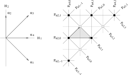
Figure 1: Root vectors and a Weyl domain in SO(5) (Sp(2)). Filled circles are central lattice points with SO(5) (Sp(2)) enhancement. Every unfilled circle has the centralizer SO(4) (${\rm SU}(2)\times{\rm SU}(2)$).

This can be directly checked by using the matrix $X$ in Eq. (15). Suppose ${\rm SO}(5)$ is acting on the space with coordinates $(x_{1},\cdots,x_{5})$. Denote an $n\times n$ submatrix of a parent $5\times 5$ matrix by $(i_{1},\cdots,i_{n})$ indicating the subspace $(x_{i_{1}},\cdots,x_{i_{n}})$ on which the submatrix is acting. As shown in appendix B.3 in [5], ${\rm SU}(2)_{\alpha_{1}}$ for a long root is generated by two ${\bf 2}$’s of SU(2) specified by $(1,2)$, $(4,5)$ blocks, whereas ${\rm SU}(2)_{\alpha_{2}}$ for a short root is generated by a ${\bf 3}$ of SU(2) given by $(1,3,5)$ block. Similarly, ${\rm SU}(2)_{\alpha_{3}}$ is generated by two ${\bf 2}$’s of $(1,4)$, $(2,5)$ blocks, while ${\rm SU}(2)_{\alpha_{4}}$ is generated by a ${\bf 3}$ of $(2,3,4)$ block. For the point $(\psi_{1},\psi_{2})=(1,1)$, $h\equiv e^{2\pi iX}$ is now given by the diagonal matrix:

$$h~{}=~{}{\rm diag}(-1,-1,1,-1,-1)$$ (17)

which is proportional to the identity matrix both in $(1,2)$, $(4,5)$ blocks and in $(1,4)$, $(2,5)$ blocks, so that both ${\rm SU}(2)_{\alpha_{1}}$ and ${\rm SU}(2)_{\alpha_{3}}$ become symmetry of the $h$.

However, the same $h$ contains the identity matrix in $(1,2,4,5)$ block also. Thus the centralizer ${\cal Z}(h)$ seems to be SO(4) acting on $(1,2,4,5)$ block, rather than ${\rm SU}(2)\times{\rm SU}(2)$. As we will see later, the centralizer generated by two long roots $\alpha_{1}$ and $\alpha_{3}$ depends on the global topology of the parent group $G$, namely $\pi_{1}(G)=\{0\}$ or ${\bf Z}_{2}$. For $G={\rm Sp}(2)$, $\alpha_{1}$ and $\alpha_{3}$ generate ${\rm Spin}(4)\cong{\rm SU}(2)\times{\rm SU}(2)$, whereas for $G={\rm SO}(5)$ they generate SO(4).

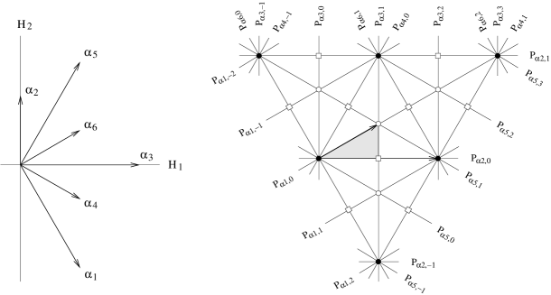
Figure 2: Root vectors and a Weyl domain in G₂. Filled circles are central lattice points with $G_{2}$ enhancement. Every unfilled circle has the centralizer SU(3). The intersection points indicated by squares have ${\rm SU}(2)\times{\rm SU}(2)$ enhancement.

$G_{2}$: The fundamental representation of $G_{2}$ is 7-dimensional and ${\bf 7}$ of $G_{2}$ goes to ${\bf 3+\bar{3}+1}$ in an SU(3) subgroup. As shown in [8], the 14 generators of $G_{2}$ are given by certain linear combinations of the 21 generators of ${\rm SO}(7)$. After appropriate diagonalization, the first 8 generators are given by 7$\times$7 matrices which are direct sum of $\lambda_{a}\oplus\,[-\lambda_{a}]^{T}\oplus\,0$ where $\lambda_{a}$’s are Gell-Mann matrices as expected from the branching rule ${\bf 7\to 3+\bar{3}+1}$ (See appendix B.5 in [5] also). Recalling that SU(3) is the regular maximal subgroup of $G_{2}$, one can choose Cartan generators of $G_{2}$ as the same as those of SU(3), namely

$$H_{1}=\frac{1}{\sqrt{2}}\left(\lambda_{3}\oplus[-\lambda_{3}]^{T}\oplus 0\right),\quad H_{2}=\frac{1}{\sqrt{2}}\left(\lambda_{8}\oplus[-\lambda_{8}]^{T}\oplus 0\right).$$ (18)

The simple roots and fundamental weights of ${\mathfrak{g}}_{2}$ are

$$\begin{array}[]{ll}\vec{\alpha}_{1}=\left(\displaystyle\frac{\mathstrut 1}{\mathstrut\sqrt{2}},-\sqrt{\displaystyle\frac{\mathstrut 3}{\mathstrut 2}}\,\right),&\vec{\alpha}_{2}=\left(0,~{}\sqrt{\displaystyle\frac{\mathstrut 2}{\mathstrut 3}}\,\right),\vspace{12pt}\\ \vec{\mu}_{1}=(\sqrt{2},~{}0),&\vec{\mu}_{2}=\left(\displaystyle\frac{\mathstrut 1}{\mathstrut\sqrt{2}},~{}\displaystyle\frac{\mathstrut 1}{\mathstrut\sqrt{6}}\right).\end{array}$$ (21)

All other positive roots are $\vec{\alpha}_{3}=2\vec{\alpha}_{1}+3\vec{\alpha}_{2}$, $\vec{\alpha}_{4}=\vec{\alpha}_{1}+\vec{\alpha}_{2}$, $\vec{\alpha}_{5}=\vec{\alpha}_{1}+3\vec{\alpha}_{2}$, $\vec{\alpha}_{6}=\vec{\alpha}_{1}+2\vec{\alpha}_{2}$. We notice that $\vec{\alpha}_{1}$, $\vec{\alpha}_{3}$, $\vec{\alpha}_{5}$ are long roots with length $\sqrt{2}$, while $\vec{\alpha}_{2}$, $\vec{\alpha}_{4}$, $\vec{\alpha}_{6}$ are short roots with length $\sqrt{2/3}$ (See figure 2).

For non-simple roots $\alpha_{m}$’s ($m=3,\cdots,6$), $\psi_{m}$’s are given by

$$\psi_{3}=2\psi_{1}+\psi_{2},\quad\psi_{5}=\psi_{1}+\psi_{2},\quad\psi_{4}=3\psi_{1}+\psi_{2},\quad\psi_{6}=3\psi_{1}+2\psi_{2}.$$ (22)

Notice that the long to short root ratio is 3 so that $l_{1}=1$, $l_{2}=3$. The symmetry enhancement lines are given by $\psi_{l}\in{\bf Z}$ for $l=1$, 3, 5 and $\psi_{s}\in 3{\bf Z}$ for $s=2$, 4, 6. A unit cell of central lattice is the parallelogram spanned by $\vec{\mu}_{1}$ and $3\vec{\mu}_{2}$ while the fundamental domain is surrounded by $P_{\alpha_{1},\,0}$, $P_{\alpha_{2},\,0}$, $P_{\alpha_{3},\,1}$. The fundamental domain (or Weyl domain) is 1/12 of the unit cell as shown in figure 2.

All the long roots, $\alpha_{1}$, $\alpha_{3}$, $\alpha_{5}$, compose an SU(3) subgroup of $G_{2}$ as shown in figure 2. Hence every intersection point where only three lines of long root enhancement meet has a symmetry group SU(3) as depicted by circles in figure 2. The corresponding D-brane becomes 6-dimensional one given by $G_{2}/{\rm SU}(3)$. We also recognize that all the short roots $\alpha_{2}$, $\alpha_{4}$, $\alpha_{6}$ compose another SU(3) subgroup of $G_{2}$. However, every intersection point of short root enhancement lines is necessarily located on the central lattice of $G_{2}$ (filled circles in figure 2) and therefore has the symmetry group $G_{2}$, not SU(3). Finally, we can choose three pairs of long and short roots orthogonal to each other, namely $(\alpha_{1},\alpha_{6})$, $(\alpha_{3},\alpha_{2})$, $(\alpha_{5},\alpha_{4})$. These pairs correspond to the intersection points depicted by squares in figure 2 where the symmetry group is enhanced to ${\rm SU}(2)\times{\rm SU}(2)$.

4. Classical moduli space and global issues

We have seen that symmetry enhancement is related to the central lattice. Now we introduce two other lattices, namely the integral lattice and the co-root lattice, to define the moduli space of D-branes and discuss the global issues of it.

• Integral lattice (IL) : It is defined as the inverse image of the identity of $G$ under the exponentiation [9]. The unit cell of the integral lattice can be identified with the moduli space, since it is in one to one correspondence with the maximal torus.

• Co-root lattice (CL) : a sublattice of central lattice that is generated by the co-roots. For a root $\alpha$, corresponding co-root $\alpha^{\vee}$ is defined as $2\alpha/|\hskip 1.0pt\alpha|^{2}$. This lattice can also be defined as the image of the origin under the reflections of the hyperplanes $P_{\alpha_{i},n}$.

$B_{2}$ and $C_{2}$: The group space $B_{2}={\rm SO}(5)$ is isomorphic to $C_{2}={\rm Sp}(2)$ locally but not globally. In fact, ${\rm SO}(5)\cong{\rm Sp}(2)/{\bf Z}_{2}$. $B_{2}$ and $C_{2}$ share the same central and co-root lattices, while they have different integral lattices. It turns out that IL of $B_{2}$ is identical to the central lattice while that of $A_{2}$ or $C_{2}$ is equal to the co-root lattice. Now one can show that [9]

$$\pi_{1}(G)={\rm IL}/{\rm CL}.$$ (23)

Using Eq. (23), it is easy to show that $\pi_{1}({\rm SO}(5))={\bf Z}_{2}$, while $\pi_{1}({\rm Sp}(2))=\{0\}$. See figure 3. The two to one relation between the two groups can be understood from the fact that the inverse image of the maximal torus, or a unit cell of IL, of the Sp(2) is double size of the SO(5) when we draw them in the same plane with the same normalization where the long root length is $\sqrt{2}$.

In fact two points $X$ and $X^{\prime}$ related by translation with any short root vector are mapped to the same point in SO(5) maximal torus but different points in Sp(2) maximal torus. The difference is by $-1$ factor since $\exp(2\pi i\vec{\alpha}_{s}\cdot\vec{H})=-I$ for any short root $\alpha_{s}$ ($I$ is the identity element in Sp(2)). This is because short root vectors are elements of the integral lattice in SO(5) but not in Sp(2). Note that the central lattice is decomposed into the co-root lattice (CL) and its complement lattice (CL^′). Both CL and CL^′ compose IL in SO(5), whereas IL of Sp(2) is given by CL only. In Sp(2), CL and CL^′ are exponentiated to be different centers $I$ and $-I$, respectively. See figure 3. Thus, the ${\bf Z}_{2}$ discussed so far can be identified with the center of Sp(2) to get the group space SO(5) as an orbifold ${\rm Sp}(2)/{\bf Z}_{2}$. Things are the same for the subgroup generated by $\alpha_{1}$ and $\alpha_{3}$. They generate SO(4) if the parent group is SO(5), whereas they generate ${\rm Spin}(4)$ as a subgroup of Sp(2).

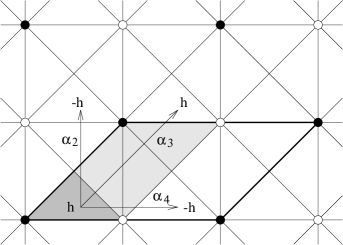
Figure 3: The integral lattice of Sp(2) consists of all the filled circles and coincides with the co-root lattice. The group manifold Sp(2) is therefore simply-connected. In SO(5), both of filled and unfilled circles compose the integral lattice, whereas the co-root lattice is given by the filled circles only.

One can also see that the ${\bf Z}_{2}$ symmetry acts on the weight space as the mirror reflections on the lines $\psi_{s}=1$ mod 2 ($s=2,4$), indicated by dashed lines in figure 1. All the CL points satisfy $\psi_{2}\pm\psi_{4}=0$ mod 4, while all the CL^′ points satisfy $\psi_{2}\pm\psi_{4}=2$ mod 4. The mirror reflections on the lines $\psi_{s}=1$ mod 2 ($s=2,4$) are given by $\psi_{s}\to 2-\psi_{s}$ ($s=2,4$), respectively. Under the reflections CL is mapped to CL^′ and vice versa. The SO(5) weight space is therefore invariant under the ${\bf Z}_{2}$ reflections. Two D-branes related by the ${\bf Z}_{2}$ reflection are different in Sp(2) but the same in SO(5). Thus we can expect that in SO(5) there exist ${\bf Z}_{2}$ invariant D-branes located on the reflection lines and such a D-brane arises as an unoriented one ${\rm SO}(5)/({\rm SO}(2)\!\times\!{\rm O}(2))$. This can be seen by looking at $h=e^{2\pi iX}$ with $X$ in Eq. (15), which gives $h={\rm diag}(z,-1,+1,-1,\bar{z})$ for the lines $\psi_{4}=1$ mod 2. Each of them has an ${\rm O}(2)$ rather than ${\rm SO}(2)$ enhancement in (2,4) block. Similarly, any of the lines $\psi_{2}=1$ mod 2 has an extra ${\bf Z}_{2}$ enhancement in $(1,5)$ block.

$G_{2}$: By looking at the explicit form of 7$\times$7 matrix $X=(\psi_{1}\vec{\mu}_{1}+\psi_{2}\vec{\mu}_{2})\cdot\vec{H}$, we notice that the integral lattice of $G_{2}$ is at the same time the central lattice depicted by filled circles in figure 2 where heperplanes of all positive roots intersect. Note also that the central lattice coincides with the co-root lattice in $G_{2}$. Eq. (23) therefore concludes that $\pi_{1}(G_{2})=\{0\}$ and the group manifold $G_{2}$ is simply-connected. If $G_{2}$ is restricted to its SU(3) subspace generated by long roots, one can think of both filled and unfilled circles in figure 2 as the central lattice points of SU(3). Then the integral lattice of $G_{2}$ is also that of the SU(3) and coincides with the SU(3) co-root lattice to conclude that $\pi_{1}({\rm SU}(3))=\{0\}$.

5. Quantum moduli space and global group structures

Quantum mechanically, the single-valuedness of the path integral of the level $k$ boundary WZW model gives two quantization conditions: one from the presence of $H$-monopoles, the other from that of $F$-monopoles. The former condition gives the quantization of level $k$, while the latter gives the condition that $k\,\vec{\psi}\cdot\vec{\alpha}_{i}^{\,\vee}$ should be an integer $n_{i}$ for all positive roots $\alpha_{i}$, or equivalently $k\,\vec{\psi}$ must be a highest weight [2, 10, 11]. The presence of $H$-monopoles also gives the condition that $k\,\vec{\psi}$ should be defined only modulo $k$.

By using Eq. (6) saying that the co-roots are dual to the fundamental weights, the stable position of a D-brane is given by

$$k\,\vec{\psi}=\sum_{i=1}^{r}n_{i}\,\vec{\mu}_{i},$$ (24)

with the coefficients $(n_{1},\cdots,n_{r})$ for simple roots. We call the set of those points satisfying Eq. (24) the quantum moduli space. As we will show shortly, the co-roots generate the homology group $H_{2}(G/T;{\bf Z})$, namely

$$H_{2}(G/T;{\bf Z})\cong{\rm CL},$$ (25)

where CL is the co-root lattice of $G$. Therefore Eq. (24) says that the highest weight $k\,\vec{\psi}$ must be an element of the cohomology group $H^{2}(G/T;{\bf Z})$ dual to $H_{2}(G/T;{\bf Z})$.

Now let us prove Eq. (25). We start from the exact homotopy sequence [12]

$$\cdots\to\pi_{2}(G)\to\pi_{2}(G/T)\to\pi_{1}(T)\to\pi_{1}(G)\to\pi_{1}(G/T)\to\pi_{0}(T)\to\cdots.$$ (26)

From $\pi_{0}(T)=\{0\}$ and $\pi_{1}(G)=\{0\}$ or ${\bf Z}_{2}$, the sequence implies that $\pi_{1}(G/T)$ is either $\{0\}$ or ${\bf Z}_{2}$. It can not be ${\bf Z}_{2}$, since it would mean that $\pi_{1}(T)=\{0\}$, which is not true. Therefore we must have $\pi_{1}(G/T)=\{0\}$. Then $\pi_{1}(T)={\bf Z}^{r}$ is classified by $\pi_{1}(G)={\bf Z}_{2}$ due to the surjectiveness of $\Phi:\pi_{1}(T)\mapsto\pi_{1}(G)$. From $\pi_{2}(G)=\{0\}$ for any compact connected Lie group $G$, $\pi_{2}(G/T)$ can be identified with its image in $\pi_{1}(T)$. Due to the exactness of the sequence, the image of $\pi_{2}(G/T)$ is equal to the kernel of $\Phi$. Thus we arrive at the non-trivial relation $\pi_{2}(G/T)={\rm Ker}\,\Phi$. Since the first non-trivial homology group and the first non-trivial homotopy group are isomorphic [12], we get $H_{2}(G/T;{\bf Z})={\rm Ker}\,\Phi$. Every unit cell of the integral lattice of $G$ is exponentiated to be the same maximal torus $T\subset G$ and it is obvious $\pi_{1}(T)\cong{\rm IL}$. Recall $\pi_{1}(G)\cong{\rm IL/CL}$ as shown in Eq. (23). Then the surjective mapping $\Phi$ can be rewritten as

$$\Phi:{\rm IL}\mapsto{\rm IL/CL}$$ (27)

which immediately says ${\rm Ker}\,\Phi\cong{\rm CL}$ and we arrive at Eq. (25).

Although the condition (24) arises in the same way for SO(5) and Sp(2), its meaning is different between two cases. The condition says that half the Weyl domain enclosed by three lines $\psi_{1}=0$, $\psi_{2}=0$, $\psi_{4}=1$ is discretized into a set of stable points. This can be seen by setting $n_{4}=k$ in $k\,\psi_{4}=n_{4}$. Hence the D-branes located on the ${\bf Z}_{2}$ reflection lines $\psi_{s}=1$ mod 2 ($s=2,4$) can be stable quantum mechanically. Such a D-brane arises as an unoriented one ${\rm SO}(5)/({\rm SO}(2)\times{\rm O}(2))$ in SO(5), while as a generic one ${\rm Sp}(2)/{\rm U}(1)^{2}$ in Sp(2). Things are the same when we compare SO($N$)’s with their covering groups Spin($N$)’s ($N\geq 3$). For SO(3) as $B_{1}$ generated by a single short root, an unoriented D-brane ${\rm SO}(3)/{\rm O}(2)$ can be stable as shown in [4].

So far our discussion on quantum moduli space is just based on the (co)homological consideration. According to the CFT analysis, the condition (24) must be corrected in two ways [2]. First, the level $k$ must be shifted to $k+x$, where $x$ is the dual Coxeter number of the group $G$ and is given by $N-2$ for SO($N$), $N+1$ for Sp($N$), 9 for $F_{4}$, 4 for $G_{2}$. Second, the highest weight $k\,\vec{\psi}$ must be shifted by the Weyl vector $\vec{\rho}$, that is defined as half the sum of all positive roots. Thus the condition (24) is corrected to be [2]

$$(k+x)\,\vec{\psi}=\sum_{i=1}^{r}n_{i}\,\vec{\mu}_{i}+\vec{\rho}.$$ (28)

However, we should notice that the Weyl vector is always equal to the sum of all fundamental weights, that is $\vec{\rho}=\sum_{i=1}^{r}\vec{\mu}_{i}$, for any compact Lie group. Therefore the exact condition (28) is not so different from the semi-classical one (24) except for shifting $k\to k+x$ and $n_{i}\to n_{i}+1$. The singular D-branes are still allowed quantum mechanically.

6. Conclusions

In this paper, we gave a general prescription for the D-brane classification according to the D-brane position in the fundamental domain of the weight space. Utilizing the method of iterative deletion in Dynkin diagram, we constructed all the D-branes in compact non-simply-laced Lie groups. In $G_{2}$ case, we found the D6-brane $G_{2}/{\rm SU}(3)$, that is the 6-dimensional sphere embedded in ${\bf R}^{7}$ spanned by imaginary octonions [13]. We also described the global issues involved in the SO groups using the integral and co-root lattices. The group space SO(5) can be understood as an orbifold ${\rm Sp}(2)/{\bf Z}_{2}$ where ${\bf Z}_{2}$ is the center of Sp(2). The ${\bf Z}_{2}$ invariant D-brane in SO(5) arises as an unoriented D-brane ${\rm SO}(5)/({\rm SO}(2)\!\times\!{\rm O}(2))$. The semi-classical condition (24) for the quantum moduli space is not affected so much by the CFT corrections and the singular D-branes can be stable even for the finite level $k$. However, there is also another effect working at finite level: the brane world volume is not sharply localized and becomes ‘fuzzy’ as shown in [2]. It might be interesting to see how the methods of present paper can be used to discuss this effect or related quantum symmetries discussed in [14]. For future work, we may extend our analysis in this paper to the classification of twisted D-branes [2, 4] and also to D-branes in coset spaces.

Acknowledgements: This work is supported in part by KOSEF 1999-2-112-003-5. It is also supported in part by Hanyang University, Korea made in the program year of 2001. The authors are grateful to J. Fuchs for his comments on the earlier version of this paper.

References

- [1] A.Yu. Alekseev and V. Schomerus, Phys. Rev. D 60 (1999) 061901, hep-th/9812193.
- [2] G. Felder, J. Fröhlich, J. Fuchs and C. Schweigert, J. Geom. Phys. 34 (2000) 162, hep-th/9909030.
- [3] S. Stanciu, JHEP 0001 (2000) 025, hep-th/9909163.
- [4] S. Stanciu, “An illustrated guide to D-branes in SU(3),” hep-th/0111221.
- [5] T. Itoh and S.-J. Sin, “A note on singular D-branes in group manifolds,” hep-th/0206238.
- [6] N. Ishibashi, Mod. Phys. Lett. A 4 (1989) 251.
- [7] M. Kato and T. Okada, Nucl. Phys. B 499 (1997) 583, hep-th/9612148.
- [8] M. Günaydin and F. Gürsey, J. Math. Phys. 14 (1973) 1651.
- [9] J.F. Adams, “Lectures on Lie Groups,” (The University of Chicago Press, Chicago, 1969).
- [10] K. Gawȩdzki, “Conformal field theory: a case study,” hep-th/9904145.
- [11] S. Stanciu, JHEP 0010 (2000) 015, hep-th/0006145.
- [12] C. Nash and S. Sen, “Topology and Geometry for Physicists,” (Academic Press, London 1983).
- [13] M. Günaydin and N.P. Warner, Nucl. Phys. B 248 (1984) 685.
- [14] J. Pawelczyk, H. Steinacker, Nucl. Phys. B 638 (2002) 433, hep-th/0203110.